
Randomized Algorithms for Very Large-Scale Linear … Algorithms for Very Large-Scale Linear Algebra...
78
Randomized Algorithms for Very Large-Scale Linear Algebra Gunnar Martinsson The University of Colorado at Boulder Collaborators: Edo Liberty, Vladimir Rokhlin, Yoel Shkolnisky, Arthur Szlam, Joel Tropp, Mark Tygert, Franco Woolfe, ... Student: Nathan Halko (now at Spot Influence, LLC). Paper: N. Halko, P.G. Martinsson, J. Tropp. Finding structure with randomness: Probabilistic algorithms for constructing approximate matrix decompositions. SIAM Review, 53(2), 2011. Slides: Posted under the “Talks” tab on my webpage (google “Gunnar Martinsson”).
Transcript of Randomized Algorithms for Very Large-Scale Linear … Algorithms for Very Large-Scale Linear Algebra...
Randomized Algorithms for Very Large-Scale Linear Algebra
Gunnar MartinssonThe University of Colorado at Boulder
Collaborators: Edo Liberty, Vladimir Rokhlin, Yoel Shkolnisky, Arthur Szlam, Joel Tropp,Mark Tygert, Franco Woolfe, . . .
Student: Nathan Halko (now at Spot Influence, LLC).
Paper: N. Halko, P.G. Martinsson, J. Tropp. Finding structure with randomness: Probabilisticalgorithms for constructing approximate matrix decompositions. SIAM Review, 53(2), 2011.
Slides: Posted under the “Talks” tab on my webpage (google “Gunnar Martinsson”).

Objective:
Given an n× n matrix A, for a very large n (say n ∼ 106),we seek to compute a rank-k approximation, with k ≪ n (say k ∼ 102 or 103),
A ≈ E F∗ =
k∑j=1
ej f∗j .
n× n n× k k × n
Solving this problem leads to algorithms for computing:
• Eigenvectors corresponding to leading eigenvalues.(Require ej = λj fj , and fjkj=1 to be orthonormal.)
• Singular Value Decomposition (SVD) / Principal Component Analysis (PCA).(Require ejkj=1 and fjkj=1 to be orthogonal sets.)
• Spanning columns or rows.(Require ejkj=1 to be columns of A, or require f∗jkj=1 to be rows of A.)
• etc
The problem being addressed is ubiquitous in applications.
Applications:
• Statistical analysis via Principal Component Analysis.
• Fast algorithms for elliptic PDEs: more efficient Fast Multipole Methods, fast directsolvers, construction of special quadratures for corners and edges, etc.
• Data mining (machine learning, analysis of network matrices, etc).
• Diffusion geometry; a technique for constructing parameterizations on large collectionsof data points organized (modulo noise) along non-linear low-dimensional manifolds.Requires the computations of eigenvectors of graph Laplace operators.
• Nearest neighbor search for large clouds of points in high dimensional space.
• General pre-conditioners.
• Etc.

Question: Isn’t it well known how to compute standard factorizations?
Answer (perhaps a tendentious one): Yes — whenever the matrix fits in RAM.
Question: Isn’t it well known how to compute standard factorizations?
Answer (perhaps a tendentious one): Yes — whenever the matrix fits in RAM.

Review of existing methods I
For a dense n× n matrix that fits in RAM, excellent algorithms are already part of LAPACK(and Matlab, etc).
• Double precision accuracy.
• Very stable.
• O(n3) asymptotic complexity. Reasonably small constants.
• Require extensive random access to the matrix.
When the target rank k is much smaller than n, there also exist O(n2 k) methods with similarcharacteristics (the well-known Golub-Businger method, RRQR by Gu and Eisentstat, etc).
For smalla matrices the state-of-the-art is very satisfactory.For kicks, we will improve on it anyway, but this is not the main point.
aOn a standard 2012 personal computer (or cell phone ... ), “small” means n ≤ 10 000 or so.

Review of existing methods II
If the matrix is large, but can rapidly be applied to a vector (if it is sparse, or sparse inFourier space, or amenable to the FMM, etc.), so called Krylov subspace methods oftenyield excellent accuracy and speed.
The idea is to pick a starting vector ω (often a random vector), “restrict” the matrix A to thek-dimensionsal “Krylov subspace”
Span(ω, Aω, A2ω, . . . , Ak−1ω)
and compute approximate eigenvectors of the resulting matrix. Advantages:
• Very simple access to A.
• Extremely high accuracy possible.
Drawbacks:
• In standard implementations, the matrix is revisited O(k) times if a rank-k approximationis sought. (Blocked versions exist, but the convergence analysis is less developed.)
• There are numerical stability issues. These are well-studied and can be overcome, butthey make the algorithms less portable (between applications, hardware platforms, etc.).

“New” challenges in algorithmic design:
The existing state-of-the-art methods of numerical linear algebra that we have very brieflyoutlined were designed for an environment where the matrix fits in RAM and the key toperformance was to minimize the number of floating point operations required.
Currently, communication is becoming the real bottleneck:
• While clock speed is hardly improving at all anymore, the cost of a flop keeps goingdown rapidly. (Multi-core processors, GPUs, cloud computing, etc.)
• The cost of slow storage (hard drives, flash memory, etc.) is also going down rapidly.
• Communication costs are not decreasing rapidly.– Moving data from a hard-drive.– Moving data between nodes of a parallel machine. (Or cloud computer ... )– The amount of fast cache memory close to a processor is not improving much.
(In fact, it could be said to be shrinking — GPUs, multi-core, etc.)
• “Deluge of data”. Driven by ever cheaper storage and acquisition techniques. Websearch, data mining in archives of documents or photos, hyper-spectral imagery, socialnetworks, gene arrays, proteomics data, sensor networks, financial transactions, . . .

The more powerful computing machinery becomes,the more important efficient algorithm design becomes.
• Linear scaling (w.r.t. problem size, processors, etc.).
• Minimal data movement.

That randomization can be used to overcome some of the communication bottlenecks inmatrix computations has been pointed out by several authors:
C. H. Papadimitriou, P. Raghavan, H. Tamaki, and S. Vempala (2000)
A. Frieze, R. Kannan, and S. Vempala (1999, 2004)
D. Achlioptas and F. McSherry (2001)
P. Drineas, R. Kannan, M. W. Mahoney, and S. Muthukrishnan (2006a, 2006b, 2006c,2006d, etc)
S. Har-Peled (2006)
A. Deshpande and S. Vempala (2006)
S. Friedland, M. Kaveh, A. Niknejad, and H. Zare (2006)
T. Sarlós (2006a, 2006b, 2006c)
K. Clarkson, D. Woodruff (2009)
Literature survey: Halko, Martinsson, Tropp (2011).
Review of existing methods III
Examples of how randomization could be used:
• Random column/row selectionDraw at random some columns and suppose that they span the entire column space.If rows are drawn as well, then spectral properties can be estimated.Crude sampling leads to less than O(mn) complexity, but is very dangerous.
• SparsificationZero out the vast majority of the entries of the matrix. Keep a random subset of entries,and boost their magnitude to preserve “something.”
• Quantization and sparsificationRestrict the entries of the matrix to a small set of values (-1/0/1 for instance).
The methods outlined can be as fast as you like, but must necessarily have very weakperformance guarantees. They can work well for certain classes of matrices for whichadditional information is available.
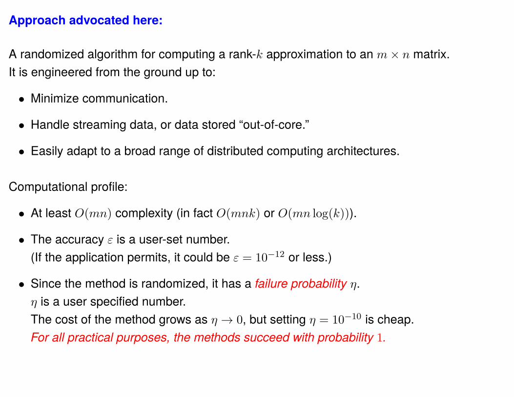
Approach advocated here:
A randomized algorithm for computing a rank-k approximation to an m× n matrix.It is engineered from the ground up to:
• Minimize communication.
• Handle streaming data, or data stored “out-of-core.”
• Easily adapt to a broad range of distributed computing architectures.
Computational profile:
• At least O(mn) complexity (in fact O(mnk) or O(mn log(k))).
• The accuracy ε is a user-set number.(If the application permits, it could be ε = 10−12 or less.)
• Since the method is randomized, it has a failure probability η.η is a user specified number.The cost of the method grows as η → 0, but setting η = 10−10 is cheap.For all practical purposes, the methods succeed with probability 1.
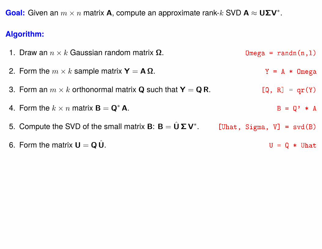
Goal: Given an m× n matrix A, compute an approximate rank-k SVD A ≈ UΣV∗.

Goal: Given an m× n matrix A, compute an approximate rank-k SVD A ≈ UΣV∗.
Algorithm:
1.
2.
3.
4. Form the k × n matrix B = Q∗A.
5. Compute the SVD of the small matrix B: B = UΣV∗.
6. Form the matrix U = QU.
Find an m× k orthonormal matrix Q such that A ≈ QQ∗A.(I.e., the columns of Q form an ON-basis for the range of A.)
Note: Steps 4 – 6 are exact; the error in the method is all in Q:
||A− U︸︷︷︸=QU
ΣV∗|| = ||A−QUΣV∗︸ ︷︷ ︸=B
|| = ||A−Q B︸︷︷︸Q∗A
|| = ||A−QQ∗A||.
Note: The classical Golub-Businger algorithm follows this pattern. It finds Q in Step 3 viadirect orthogonalization of the columns of A via, e.g., Gram-Schmidt.

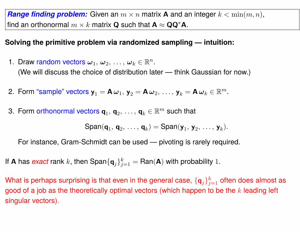
Range finding problem: Given an m× n matrix A and an integer k < min(m,n),find an orthonormal m× k matrix Q such that A ≈ QQ∗A.
Solving the primitive problem via randomized sampling — intuition:
1. Draw random vectors ω1, ω2, . . . , ωk ∈ Rn.(We will discuss the choice of distribution later — think Gaussian for now.)
2. Form “sample” vectors y1 = Aω1, y2 = Aω2, . . . , yk = Aωk ∈ Rm.
3. Form orthonormal vectors q1, q2, . . . , qk ∈ Rm such that
Span(q1, q2, . . . , qk) = Span(y1, y2, . . . , yk).
For instance, Gram-Schmidt can be used — pivoting is rarely required.
If A has exact rank k, then Spanqjkj=1 = Ran(A) with probability 1.
What is perhaps surprising is that even in the general case, qjkj=1 often does almost asgood of a job as the theoretically optimal vectors (which happen to be the k leading leftsingular vectors).

Range finding problem: Given an m× n matrix A and an integer k < min(m,n),find an orthonormal m× k matrix Q such that A ≈ QQ∗A.
Solving the primitive problem via randomized sampling — intuition:
1. Draw a random matrix Ω ∈ Rn×k.(We will discuss the choice of distribution later — think Gaussian for now.)
2. Form a “sample” matrix Y = AΩ ∈ Rm×k.
3. Form a orthonormal matrix Q ∈ Rm×k such that Y = QR.For instance, Gram-Schmidt can be used — pivoting is rarely required.
If A has exact rank k, then A = QQ∗A with probability 1.
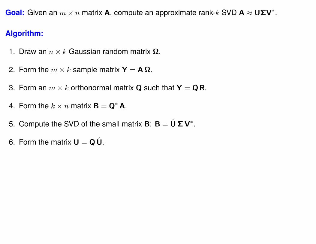
Goal: Given an m× n matrix A, compute an approximate rank-k SVD A ≈ UΣV∗.
Algorithm:
1. Draw an n× k Gaussian random matrix Ω. Omega = randn(n,l)
2. Form the m× k sample matrix Y = AΩ. Y = A * Omega
3. Form an m× k orthonormal matrix Q such that Y = QR. [Q, R] = qr(Y)
4. Form the k × n matrix B = Q∗A. B = Q' * A
5. Compute the SVD of the small matrix B: B = UΣV∗. [Uhat, Sigma, V] = svd(B)
6. Form the matrix U = QU. U = Q * Uhat
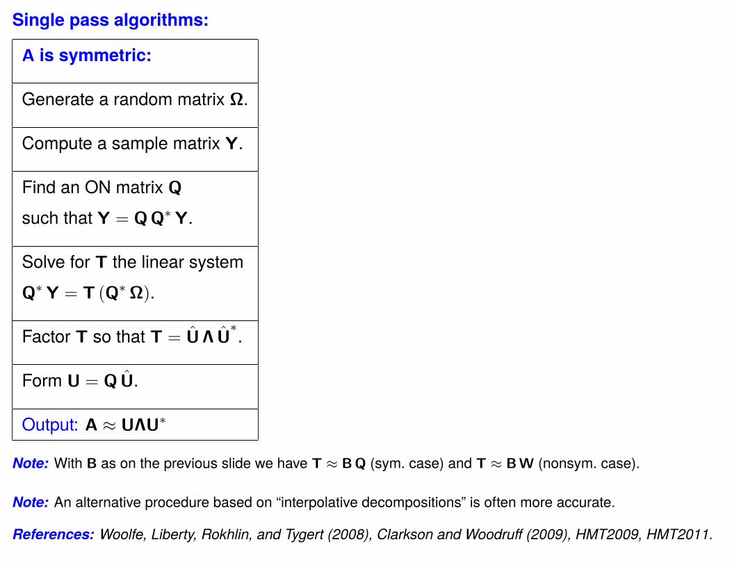
Single pass algorithms:
A is symmetric:
Generate a random matrix Ω.
Compute a sample matrix Y.
Find an ON matrix Q
such that Y = QQ∗Y.
Solve for T the linear systemQ∗Y = T (Q∗Ω).
Factor T so that T = U Λ U∗.
Form U = QU.
Output: A ≈ UΛU∗
Note: With B as on the previous slide we have T ≈ BQ (sym. case) and T ≈ BW (nonsym. case).
Note: An alternative procedure based on “interpolative decompositions” is often more accurate.
References: Woolfe, Liberty, Rokhlin, and Tygert (2008), Clarkson and Woodruff (2009), HMT2009, HMT2011.
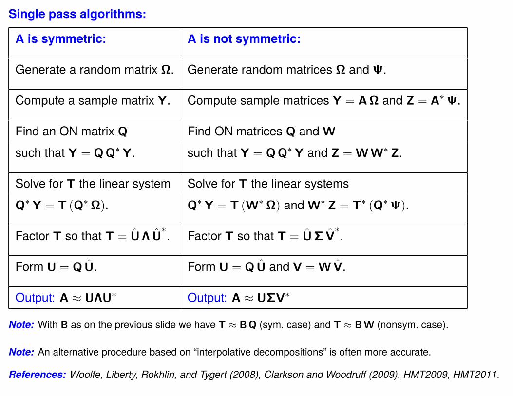
Single pass algorithms:
A is symmetric: A is not symmetric:
Generate a random matrix Ω. Generate random matrices Ω and Ψ.
Compute a sample matrix Y. Compute sample matrices Y = AΩ and Z = A∗Ψ.
Find an ON matrix Q Find ON matrices Q and W
such that Y = QQ∗Y. such that Y = QQ∗Y and Z = WW∗ Z.
Solve for T the linear system Solve for T the linear systemsQ∗Y = T (Q∗Ω). Q∗Y = T (W∗Ω) and W∗ Z = T∗ (Q∗Ψ).
Factor T so that T = U Λ U∗. Factor T so that T = UΣ V
∗.
Form U = QU. Form U = QU and V = WV.
Output: A ≈ UΛU∗ Output: A ≈ UΣV∗
Note: With B as on the previous slide we have T ≈ BQ (sym. case) and T ≈ BW (nonsym. case).
Note: An alternative procedure based on “interpolative decompositions” is often more accurate.
References: Woolfe, Liberty, Rokhlin, and Tygert (2008), Clarkson and Woodruff (2009), HMT2009, HMT2011.
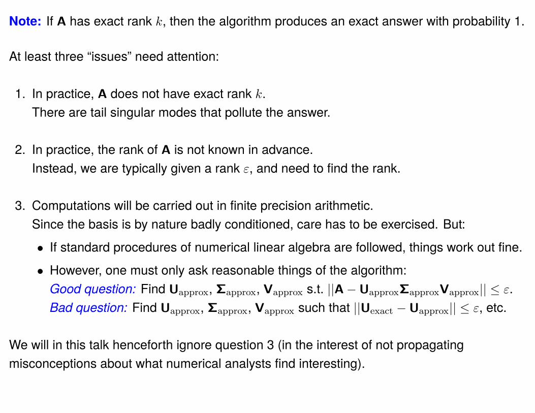
Note: If A has exact rank k, then the algorithm produces an exact answer with probability 1.
At least three “issues” need attention:
1. In practice, A does not have exact rank k.There are tail singular modes that pollute the answer.
2. In practice, the rank of A is not known in advance.Instead, we are typically given a rank ε, and need to find the rank.
3. Computations will be carried out in finite precision arithmetic.Since the basis is by nature badly conditioned, care has to be exercised. But:
• If standard procedures of numerical linear algebra are followed, things work out fine.
• However, one must only ask reasonable things of the algorithm:Good question: Find Uapprox, Σapprox, Vapprox s.t. ||A−UapproxΣapproxVapprox|| ≤ ε.Bad question: Find Uapprox, Σapprox, Vapprox such that ||Uexact −Uapprox|| ≤ ε, etc.
We will in this talk henceforth ignore question 3 (in the interest of not propagatingmisconceptions about what numerical analysts find interesting).
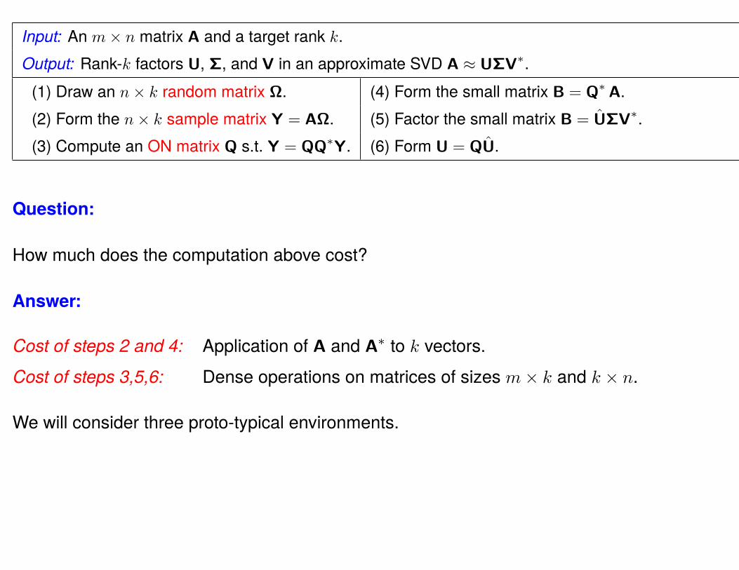
Input: An m× n matrix A and a target rank k.Output: Rank-k factors U, Σ, and V in an approximate SVD A ≈ UΣV∗.
(1) Draw an n× k random matrix Ω. (4) Form the small matrix B = Q∗ A.(2) Form the n× k sample matrix Y = AΩ. (5) Factor the small matrix B = UΣV∗.(3) Compute an ON matrix Q s.t. Y = QQ∗Y. (6) Form U = QU.
Question:
How much does the computation above cost?
Answer:
Cost of steps 2 and 4: Application of A and A∗ to k vectors.Cost of steps 3,5,6: Dense operations on matrices of sizes m× k and k × n.
We will consider three proto-typical environments.

Input: An m× n matrix A and a target rank k.Output: Rank-k factors U, Σ, and V in an approximate SVD A ≈ UΣV∗.
(1) Draw an n× k random matrix Ω. (4) Form the small matrix B = Q∗ A.(2) Form the n× k sample matrix Y = AΩ. (5) Factor the small matrix B = UΣV∗.(3) Compute an ON matrix Q s.t. Y = QQ∗Y. (6) Form U = QU.
Cost of steps 2 and 4: Application of A and A∗ to k vectors.Cost of steps 3,5,6: Dense operations on matrices of sizes m× k and k × n.
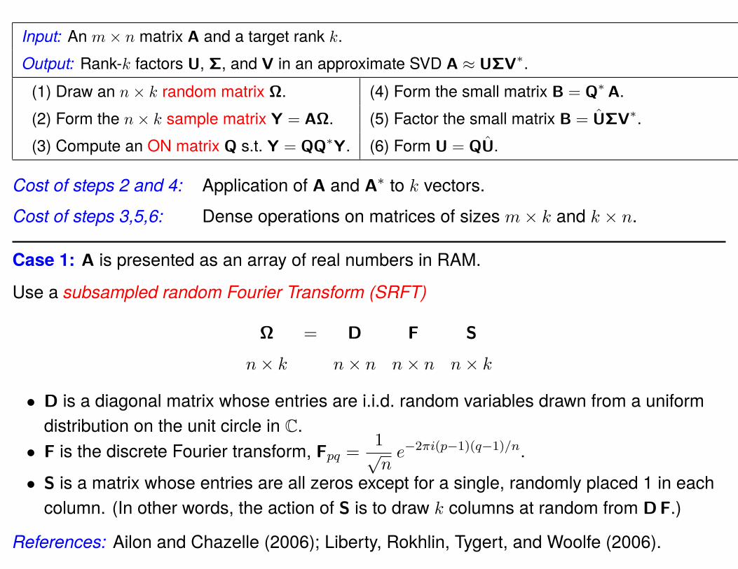
Case 1: A is presented as an array of real numbers in RAM.
Cost is dominated by the 2mnk flops required for steps 2 and 4.
The O(mnk) flop count is the same as that of standard methods such as Golub-Businger.However, the algorithm above requires no random access to the matrix A — the data isretrieved in two passes. (One pass in the modified version.)
Remark 1: Improved data access leads to a moderate gain (×2) in execution time.
Remark 2: Using a special structured random sampling matrix (for instance, a “subsampledrandom Fourier transform” / “fast Johnson-Lindenstrauss transform”), substantial gain inexecution time, and asymptotic complexity of O(mn log(k)) can be achieved.
Input: An m× n matrix A and a target rank k.Output: Rank-k factors U, Σ, and V in an approximate SVD A ≈ UΣV∗.
(1) Draw an n× k random matrix Ω. (4) Form the small matrix B = Q∗ A.(2) Form the n× k sample matrix Y = AΩ. (5) Factor the small matrix B = UΣV∗.(3) Compute an ON matrix Q s.t. Y = QQ∗Y. (6) Form U = QU.
Cost of steps 2 and 4: Application of A and A∗ to k vectors.Cost of steps 3,5,6: Dense operations on matrices of sizes m× k and k × n.
Case 1: A is presented as an array of real numbers in RAM.
Use a subsampled random Fourier Transform (SRFT)
Ω = D F S
n× k n× n n× n n× k
• D is a diagonal matrix whose entries are i.i.d. random variables drawn from a uniformdistribution on the unit circle in C.
• F is the discrete Fourier transform, Fpq =1√ne−2πi(p−1)(q−1)/n.
• S is a matrix whose entries are all zeros except for a single, randomly placed 1 in eachcolumn. (In other words, the action of S is to draw k columns at random from DF.)
References: Ailon and Chazelle (2006); Liberty, Rokhlin, Tygert, and Woolfe (2006).

Step (4) involves a second O(mnk) cost, but this can be eliminated via a variation of therandomized sampling process that samples both the column space and the row space:
Given an m× n matrix A, find U, V, Σ of rank k such that A ≈ UΣV∗.
1. Choose an over-sampling parameter p and set ℓ = k + p. (Say p = k so ℓ = 2k.)
2. Generate SRFT’s Ω and Ψ of sizes n× ℓ, and m× ℓ.
3. Form the sample matrices Y = AΩ and Z = A∗Ψ.
4. Find ON matrices Q and W such that Y = QQ∗Y and Z = WW∗ Z.
5. Solve for the k × k matrix T the systems Q∗Y = T (W∗Ω) and W∗ Z = T∗ (Q∗Ψ).
6. Compute the SVD of the small matrix T = UΣ V∗ (and truncate if desired).
7. Form U = QU and V = WV.
Observation 1: Forming AΩ and A∗Ψ in Step 2 has cost O(mn log(k)) since ℓ ∼ k.
Observation 2: All other steps cost at most O((m+ n) k2).
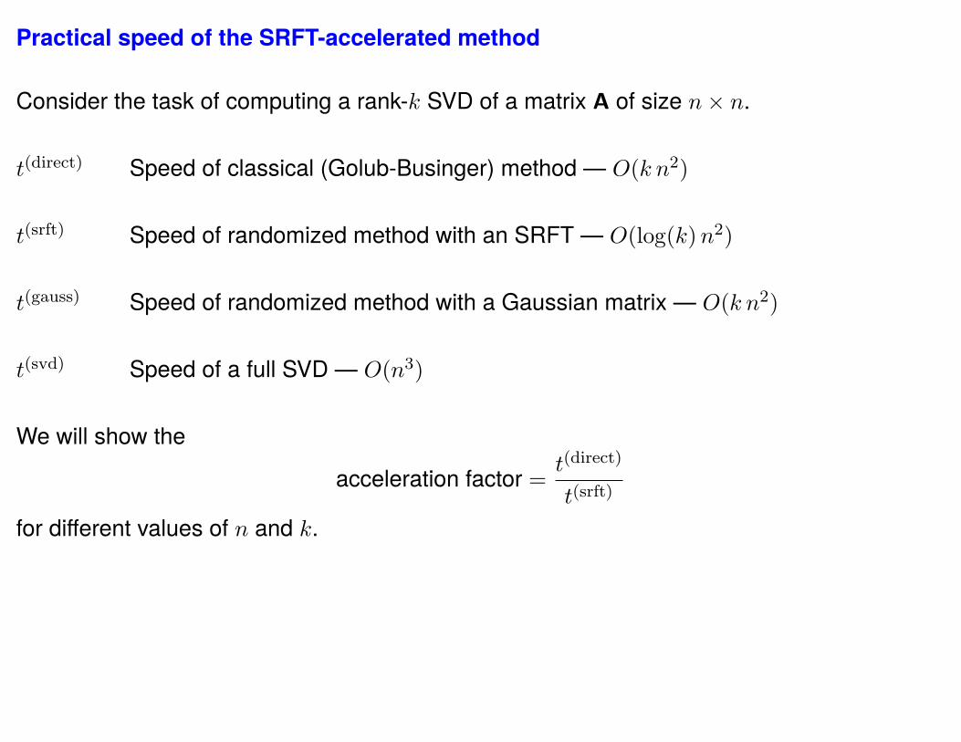
Practical speed of the SRFT-accelerated method
Consider the task of computing a rank-k SVD of a matrix A of size n× n.
t(direct) Speed of classical (Golub-Businger) method — O(k n2)
t(srft) Speed of randomized method with an SRFT — O(log(k)n2)
t(gauss) Speed of randomized method with a Gaussian matrix — O(k n2)
t(svd) Speed of a full SVD — O(n3)
We will show the
acceleration factor = t(direct)
t(srft)
for different values of n and k.
101
102
103
0
1
2
3
4
5
6
7
101
102
103
0
1
2
3
4
5
6
7
101
102
103
0
1
2
3
4
5
6
7
k k k
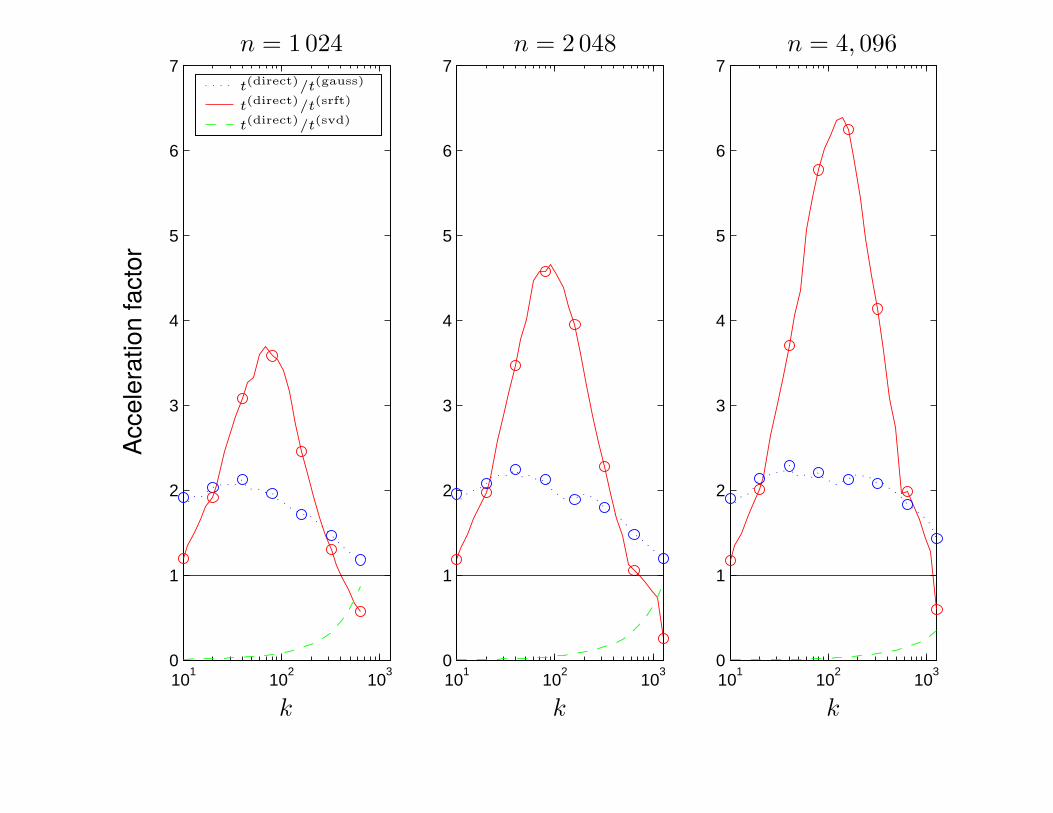
n = 1024 n = 2048 n = 4, 096
t(direct)/t(gauss)
t(direct)/t(srft)
t(direct)/t(svd)
Acce
lera
tion
fact
or

Notes:
• Significant speed-ups are achieved for common problem sizes. For instance,m = n = 2000 and k = 200 leads to a speed-up by roughly a factor of 4.
• Many other choices of random matrices have been found. (Subsampled Hadamardtransform; wavelets; random chains of Given’s rotations, etc).
• Using a randomly drawn selection of columns as a basis for the range of a matrix A isfine, provided the matrix has first been hit by a random rotation.
• Current theoretical results seem to overstate the risk of inaccurate results,at least in typical environments.
• The idea was proposed by Liberty, Rokhlin, Tygert, Woolfe (2006).– The SRFT (under the name fast Johnson-Lindenstrauss transform) was suggested
by Nir Ailon and Bernard Chazelle (2006) in a related context.– Dissertation by Edo Liberty.– Related recent work by Sarlós (on randomized regression).– Overdetermined linear least-squares regression: Rokhlin and Tygert (2008).

Input: An m× n matrix A and a target rank k.Output: Rank-k factors U, Σ, and V in an approximate SVD A ≈ UΣV∗.
(1) Draw an n× k random matrix Ω. (4) Form the small matrix B = Q∗ A.(2) Form the n× k sample matrix Y = AΩ. (5) Factor the small matrix B = UΣV∗.(3) Compute an ON matrix Q s.t. Y = QQ∗Y. (6) Form U = QU.
Cost of steps 2 and 4: Application of A and A∗ to k vectors.Cost of steps 3,5,6: Dense operations on matrices of sizes m× k and k × n.
Case 2: A is presented as an array of real numbers in slow memory — on “disk”.
In this case, standard methods such as Golub-Businger become prohibitively slow due tothe random access requirements on the data.
However, the method described above works just fine. (Recall: Two passes only!)
Limitation 1: Matrices of size m× k and k × n must fit in RAM.
Limitation 2: For matrices whose singular values decay slowly (as is typical in thedata-analysis environment), the method above is typically not accurate enough.Higher accuracy can be bought at modest cost — we will return to this point.


Input: An m× n matrix A and a target rank k.Output: Rank-k factors U, Σ, and V in an approximate SVD A ≈ UΣV∗.
(1) Draw an n× k random matrix Ω. (4) Form the small matrix B = Q∗ A.(2) Form the n× k sample matrix Y = AΩ. (5) Factor the small matrix B = UΣV∗.(3) Compute an ON matrix Q s.t. Y = QQ∗Y. (6) Form U = QU.
Cost of steps 2 and 4: Application of A and A∗ to k vectors.Cost of steps 3,5,6: Dense operations on matrices of sizes m× k and k × n.
Case 3: A and A∗ admit fast matrix-vector multiplication.
In this case, the “standard” method is some variation of Krylov methods such as Lanczos (orArnoldi for non-symmetric matrices) whose cost TKrylov satisfy:
TKrylov ∼ k Tmat-vec-mult + O(k2 (m+ n))︸ ︷︷ ︸With full “reorthogonalization”.
.
The asymptotic cost of the randomized scheme is the same; its advantage is again in howthe data is accessed — the k matrix-vector multiplies can be executed in parallel.
The method above is in important environments less accurate than Arnoldi,but this can be fixed while compromising only slightly on the pass-efficiency.

Theory

Input: An m× n matrix A and a target rank k.Output: Rank-k factors U, Σ, and V in an approximate SVD A ≈ UΣV∗.
(1) Draw an n× k random matrix Ω. (4) Form the small matrix B = Q∗ A.(2) Form the n× k sample matrix Y = AΩ. (5) Factor the small matrix B = UΣV∗.(3) Compute an ON matrix Q s.t. Y = QQ∗Y. (6) Form U = QU.
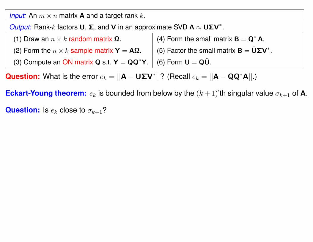
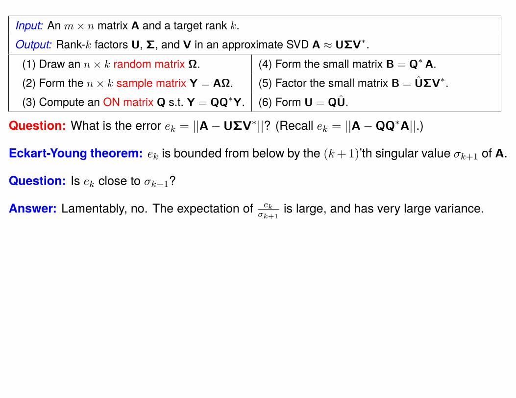
Question: What is the error ek = ||A−UΣV∗||? (Recall ek = ||A−QQ∗A||.)
Input: An m× n matrix A and a target rank k.Output: Rank-k factors U, Σ, and V in an approximate SVD A ≈ UΣV∗.
(1) Draw an n× k random matrix Ω. (4) Form the small matrix B = Q∗ A.(2) Form the n× k sample matrix Y = AΩ. (5) Factor the small matrix B = UΣV∗.(3) Compute an ON matrix Q s.t. Y = QQ∗Y. (6) Form U = QU.
Question: What is the error ek = ||A−UΣV∗||? (Recall ek = ||A−QQ∗A||.)
Eckart-Young theorem: ek is bounded from below by the (k+1)’th singular value σk+1 of A.
Question: Is ek close to σk+1?
Answer: Lamentably, no. The expectation of ekσk+1
is large, and has very large variance.
Remedy: Over-sample slightly. Compute k+p samples from the range of A.It turns out that p = 5 or 10 is often sufficient. p = k is almost always more than enough.
Input: An m× n matrix A, a target rank k, and an over-sampling parameter p (say p = 5).Output: Rank-(k + p) factors U, Σ, and V in an approximate SVD A ≈ UΣV∗.
(1) Draw an n× (k + p) random matrix Ω. (4) Form the small matrix B = Q∗ A.(2) Form the n× (k + p) sample matrix Y = AΩ. (5) Factor the small matrix B = UΣV∗.(3) Compute an ON matrix Q s.t. Y = QQ∗Y. (6) Form U = QU.

THEORY — Overview:
Let A denote an m× n matrix with singular values σjmin(m,n)j=1 .
Let k denote a target rank and let p denote an over-sampling parameter. Set ℓ = k + p.
Let Ω denote an n× ℓ “test matrix”, and let Q denote the m× ℓ matrix Q = orth(AΩ).
We seek to bound the error ek = ek(A,Ω) = ||A−QQ∗A||, which is a random variable.
1. Make no assumption on Ω. Construct a deterministic bound of the form
||A−QQ∗A|| ≤ · · ·A · · ·Ω · · ·
2. Assume Ω is drawn from a normal Gaussian distribution.Take expectations of the deterministic bound to attain a bound of the form
E[||A−QQ∗A||
]≤ · · ·A · · ·
3. Assume Ω is drawn from a normal Gaussian distribution.Take expectations of the deterministic bound conditioned on “bad behavior” in Ω to get
||A−QQ∗A|| ≤ · · ·A · · ·
that hold with probability at least · · · .
4. Brief comments about the case where Ω is an SRFT.
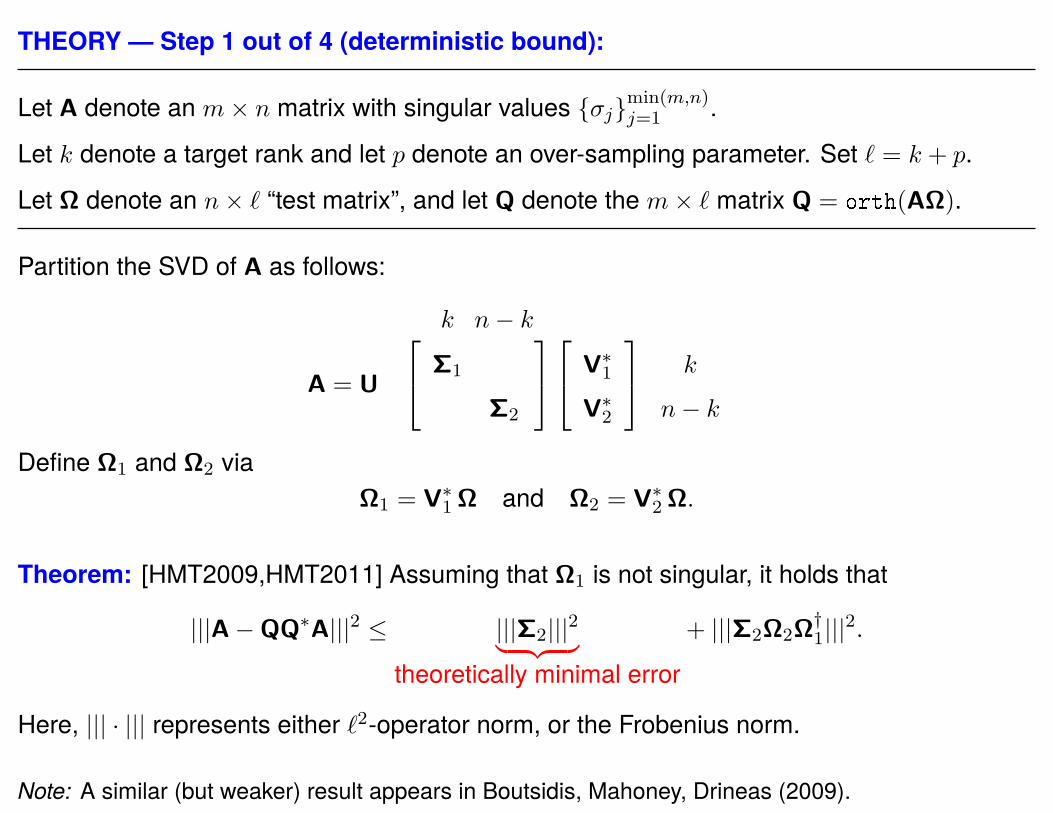
THEORY — Step 1 out of 4 (deterministic bound):
Let A denote an m× n matrix with singular values σjmin(m,n)j=1 .
Let k denote a target rank and let p denote an over-sampling parameter. Set ℓ = k + p.
Let Ω denote an n× ℓ “test matrix”, and let Q denote the m× ℓ matrix Q = orth(AΩ).
Partition the SVD of A as follows:
k n− k
A = U
Σ1
Σ2
V∗1
V∗2
k
n− k
Define Ω1 and Ω2 viaΩ1 = V∗
1Ω and Ω2 = V∗2Ω.
Theorem: [HMT2009,HMT2011] Assuming that Ω1 is not singular, it holds that
|||A−QQ∗A|||2 ≤ |||Σ2|||2︸ ︷︷ ︸theoretically minimal error
+ |||Σ2Ω2Ω†1|||
2.
Here, ||| · ||| represents either ℓ2-operator norm, or the Frobenius norm.
Note: A similar (but weaker) result appears in Boutsidis, Mahoney, Drineas (2009).

Recall: A = U
Σ1 0
0 Σ2
V∗1
V∗2
,
Ω1
Ω2
=
V∗1Ω
V∗2Ω
, Y = AΩ, P projn onto Ran(Y).
Thm: Suppose Σ1Ω1 has full rank. Then ||A− PA||2 ≤ ||Σ2||2 + ||Σ2Ω2Ω†1||
2.
Proof: The problem is rotationally invariant ⇒ We can assume U = I and so A = ΣV∗.
Simple calculation: ||(I− P)A||2 = ||A∗(I− P)2A|| = ||Σ(I− P)Σ||.
Ran(Y) = Ran
Σ1Ω1
Σ2Ω2
= Ran
I
Σ2Ω2Ω†1Σ1
Σ1Ω1
= Ran
I
Σ2Ω2Ω†1Σ1
Set F = Σ2Ω2Ω
†1Σ1. Then P =
I
F
(I+ F∗F)−1[I F∗].
Use properties of psd matrices: I− P 4 · · · 4
F∗F −(I+ F∗F)−1F∗
−F(I+ F∗F)−1 I
Conjugate by Σ to get Σ(I− P)Σ 4
Σ1F∗FΣ1 −Σ1(I+ F∗F)−1F∗Σ2
−Σ2F(I+ F∗F)−1Σ1 Σ22
Diagonal dominance: ||Σ(I− P)Σ|| ≤ ||Σ1F
∗FΣ1||+ ||Σ22|| = ||Σ2Ω2Ω
†1||2 + ||Σ2||2.
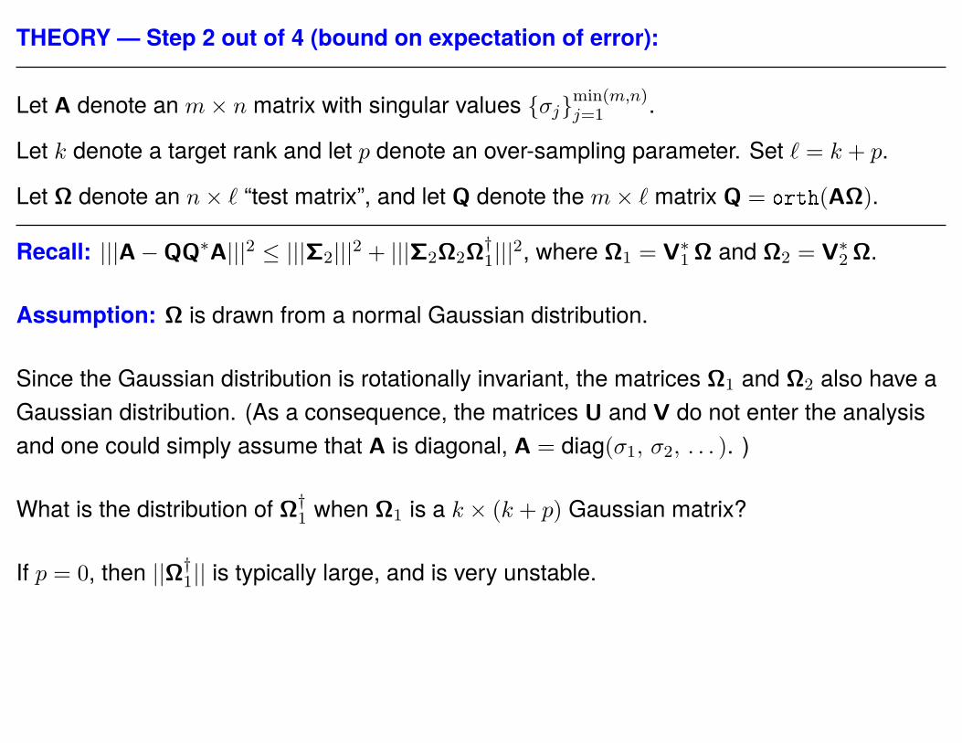
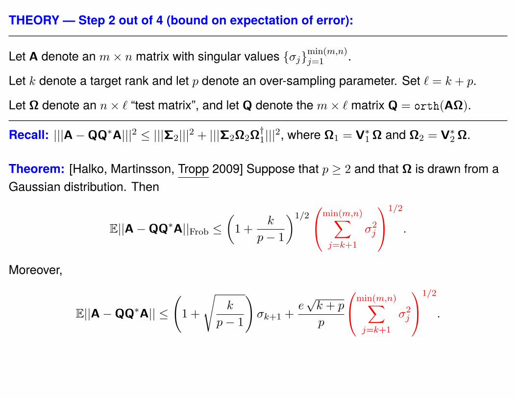
THEORY — Step 2 out of 4 (bound on expectation of error):
Let A denote an m× n matrix with singular values σjmin(m,n)j=1 .
Let k denote a target rank and let p denote an over-sampling parameter. Set ℓ = k + p.
Let Ω denote an n× ℓ “test matrix”, and let Q denote the m× ℓ matrix Q = orth(AΩ).
Recall: |||A−QQ∗A|||2 ≤ |||Σ2|||2 + |||Σ2Ω2Ω†1|||2, where Ω1 = V∗
1Ω and Ω2 = V∗2Ω.
Assumption: Ω is drawn from a normal Gaussian distribution.
Since the Gaussian distribution is rotationally invariant, the matrices Ω1 and Ω2 also have aGaussian distribution. (As a consequence, the matrices U and V do not enter the analysisand one could simply assume that A is diagonal, A = diag(σ1, σ2, . . . ). )
What is the distribution of Ω†1 when Ω1 is a k × (k + p) Gaussian matrix?
If p = 0, then ||Ω†1|| is typically large, and is very unstable.
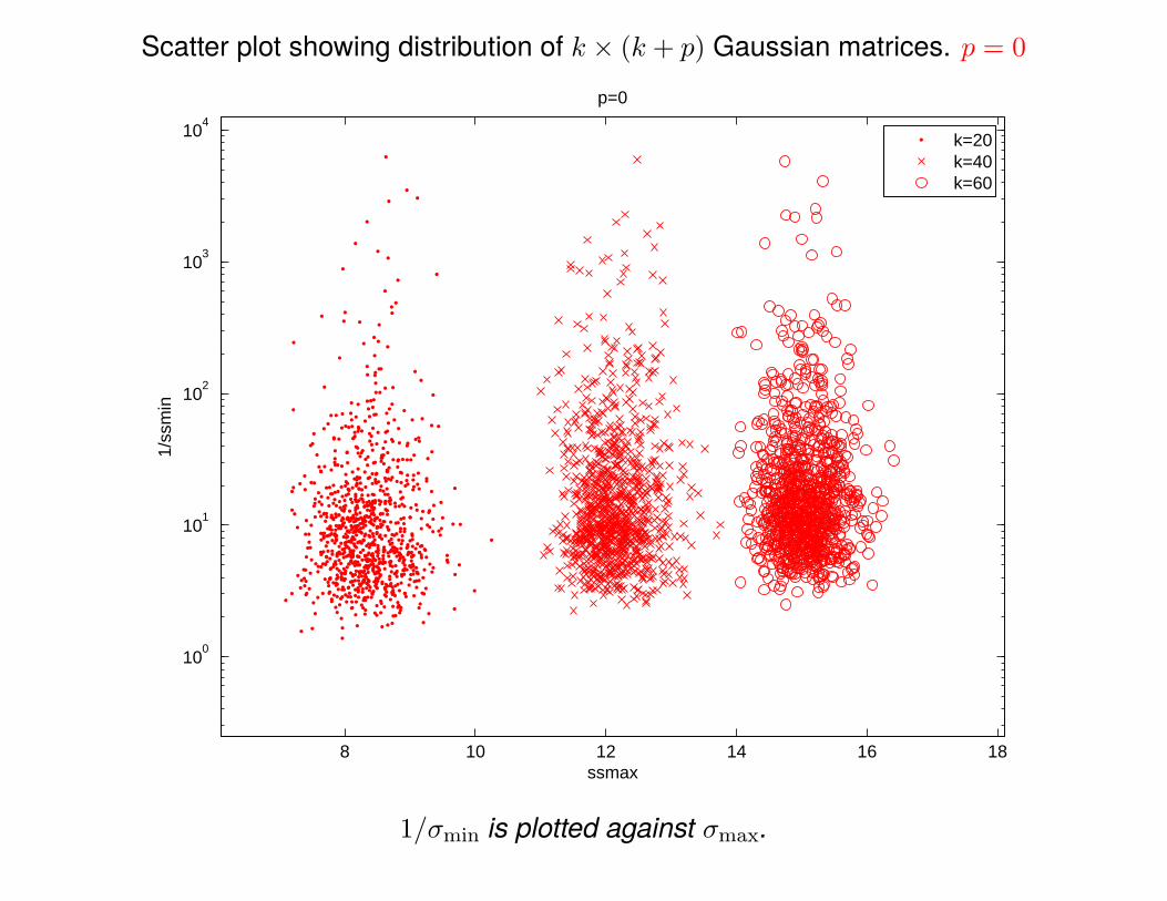
Scatter plot showing distribution of k × (k + p) Gaussian matrices. p = 0
8 10 12 14 16 18
100
101
102
103
104
ssmax
1/ss
min
p=0
k=20k=40k=60
1/σmin is plotted against σmax.

Scatter plot showing distribution of k × (k + p) Gaussian matrices. p = 2
8 10 12 14 16 18
100
101
102
103
104
ssmax
1/ss
min
p=2
k=20k=40k=60
1/σmin is plotted against σmax.
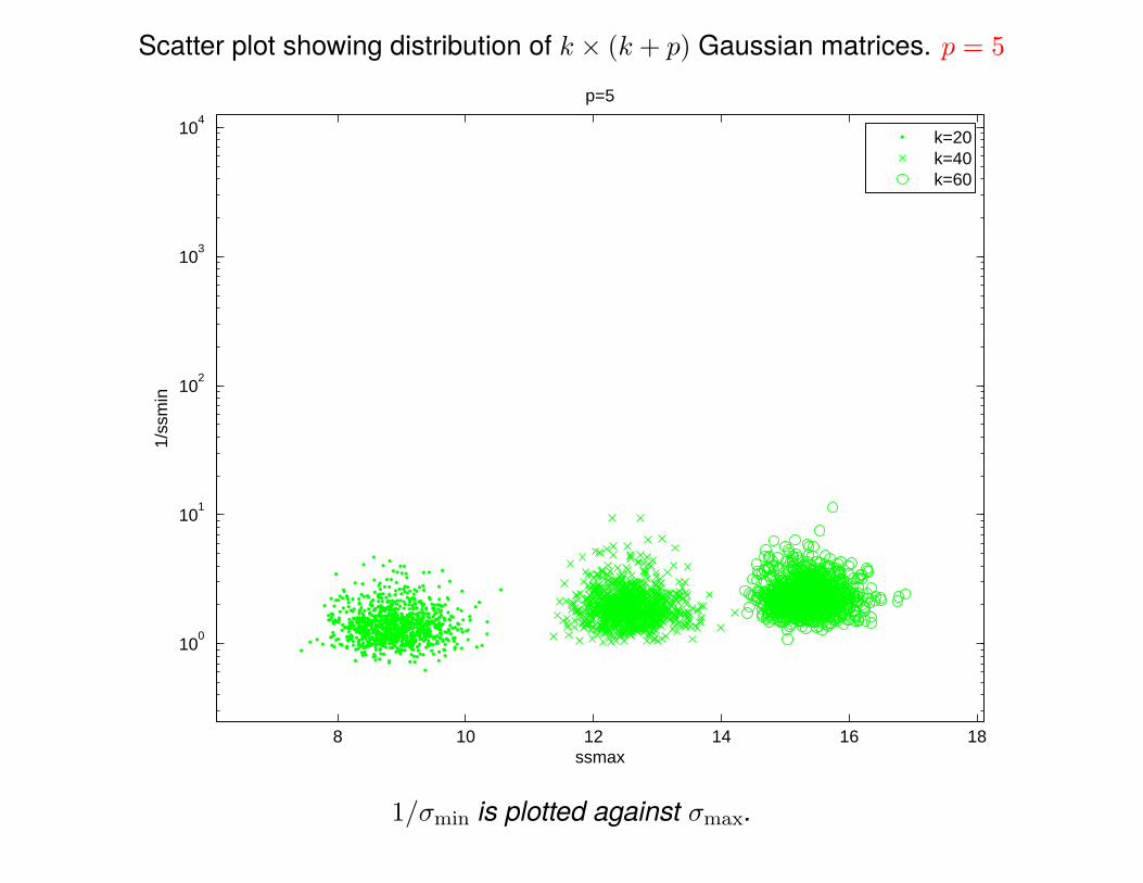
Scatter plot showing distribution of k × (k + p) Gaussian matrices. p = 5
8 10 12 14 16 18
100
101
102
103
104
ssmax
1/ss
min
p=5
k=20k=40k=60
1/σmin is plotted against σmax.

Scatter plot showing distribution of k × (k + p) Gaussian matrices. p = 10
8 10 12 14 16 18
100
101
102
103
104
ssmax
1/ss
min
p=10
k=20k=40k=60
1/σmin is plotted against σmax.

Scatter plot showing distribution of k × (k + p) Gaussian matrices.
8 10 12 14 16 18
100
101
102
103
104
ssmax
1/ss
min
p = 0
p = 2
p = 5
p = 10
k = 20 k = 40 k = 60
1/σmin is plotted against σmax.
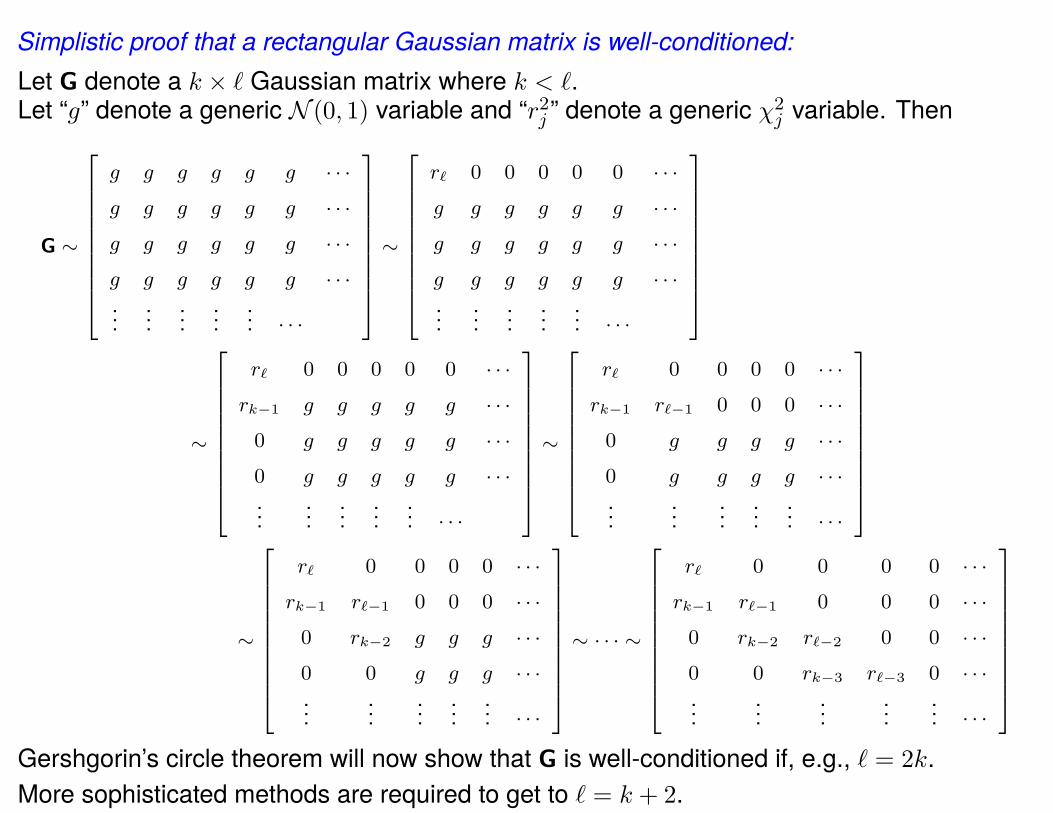
Simplistic proof that a rectangular Gaussian matrix is well-conditioned:Let G denote a k × ℓ Gaussian matrix where k < ℓ.Let “g” denote a generic N (0, 1) variable and “r2j ” denote a generic χ2
j variable. Then
G ∼
g g g g g g · · ·
g g g g g g · · ·
g g g g g g · · ·
g g g g g g · · ·...
......
...... · · ·
∼
rℓ 0 0 0 0 0 · · ·
g g g g g g · · ·
g g g g g g · · ·
g g g g g g · · ·...
......
...... · · ·
∼
rℓ 0 0 0 0 0 · · ·
rk−1 g g g g g · · ·
0 g g g g g · · ·
0 g g g g g · · ·...
......
...... · · ·
∼
rℓ 0 0 0 0 · · ·
rk−1 rℓ−1 0 0 0 · · ·
0 g g g g · · ·
0 g g g g · · ·...
......
...... · · ·
∼
rℓ 0 0 0 0 · · ·
rk−1 rℓ−1 0 0 0 · · ·
0 rk−2 g g g · · ·
0 0 g g g · · ·...
......
...... · · ·
∼ · · · ∼
rℓ 0 0 0 0 · · ·
rk−1 rℓ−1 0 0 0 · · ·
0 rk−2 rℓ−2 0 0 · · ·
0 0 rk−3 rℓ−3 0 · · ·...
......
...... · · ·
Gershgorin’s circle theorem will now show that G is well-conditioned if, e.g., ℓ = 2k.More sophisticated methods are required to get to ℓ = k + 2.
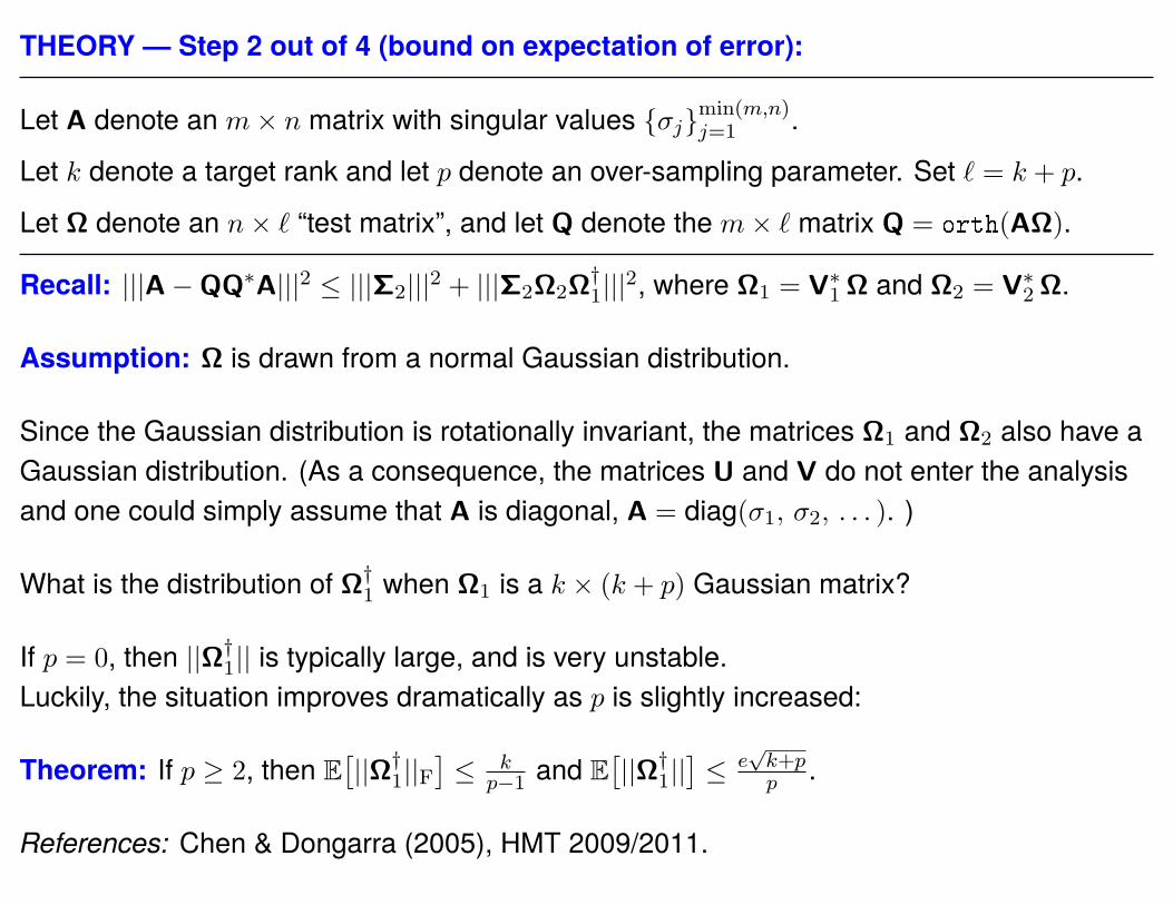
THEORY — Step 2 out of 4 (bound on expectation of error):
Let A denote an m× n matrix with singular values σjmin(m,n)j=1 .
Let k denote a target rank and let p denote an over-sampling parameter. Set ℓ = k + p.
Let Ω denote an n× ℓ “test matrix”, and let Q denote the m× ℓ matrix Q = orth(AΩ).
Recall: |||A−QQ∗A|||2 ≤ |||Σ2|||2 + |||Σ2Ω2Ω†1|||2, where Ω1 = V∗
1Ω and Ω2 = V∗2Ω.
Assumption: Ω is drawn from a normal Gaussian distribution.
Since the Gaussian distribution is rotationally invariant, the matrices Ω1 and Ω2 also have aGaussian distribution. (As a consequence, the matrices U and V do not enter the analysisand one could simply assume that A is diagonal, A = diag(σ1, σ2, . . . ). )
What is the distribution of Ω†1 when Ω1 is a k × (k + p) Gaussian matrix?
If p = 0, then ||Ω†1|| is typically large, and is very unstable.
Luckily, the situation improves dramatically as p is slightly increased:
Theorem: If p ≥ 2, then E[||Ω†
1||F]≤ k
p−1 and E[||Ω†
1||]≤ e
√k+pp .
References: Chen & Dongarra (2005), HMT 2009/2011.
THEORY — Step 2 out of 4 (bound on expectation of error):
Let A denote an m× n matrix with singular values σjmin(m,n)j=1 .
Let k denote a target rank and let p denote an over-sampling parameter. Set ℓ = k + p.
Let Ω denote an n× ℓ “test matrix”, and let Q denote the m× ℓ matrix Q = orth(AΩ).
Recall: |||A−QQ∗A|||2 ≤ |||Σ2|||2 + |||Σ2Ω2Ω†1|||2, where Ω1 = V∗
1Ω and Ω2 = V∗2Ω.
Theorem: [Halko, Martinsson, Tropp 2009] Suppose that p ≥ 2 and that Ω is drawn from aGaussian distribution. Then
E||A−QQ∗A||Frob ≤(1 +
k
p− 1
)1/2min(m,n)∑
j=k+1
σ2j
1/2
.
Moreover,
E||A−QQ∗A|| ≤
(1 +
√k
p− 1
)σk+1 +
e√k + p
p
min(m,n)∑j=k+1
σ2j
1/2
.
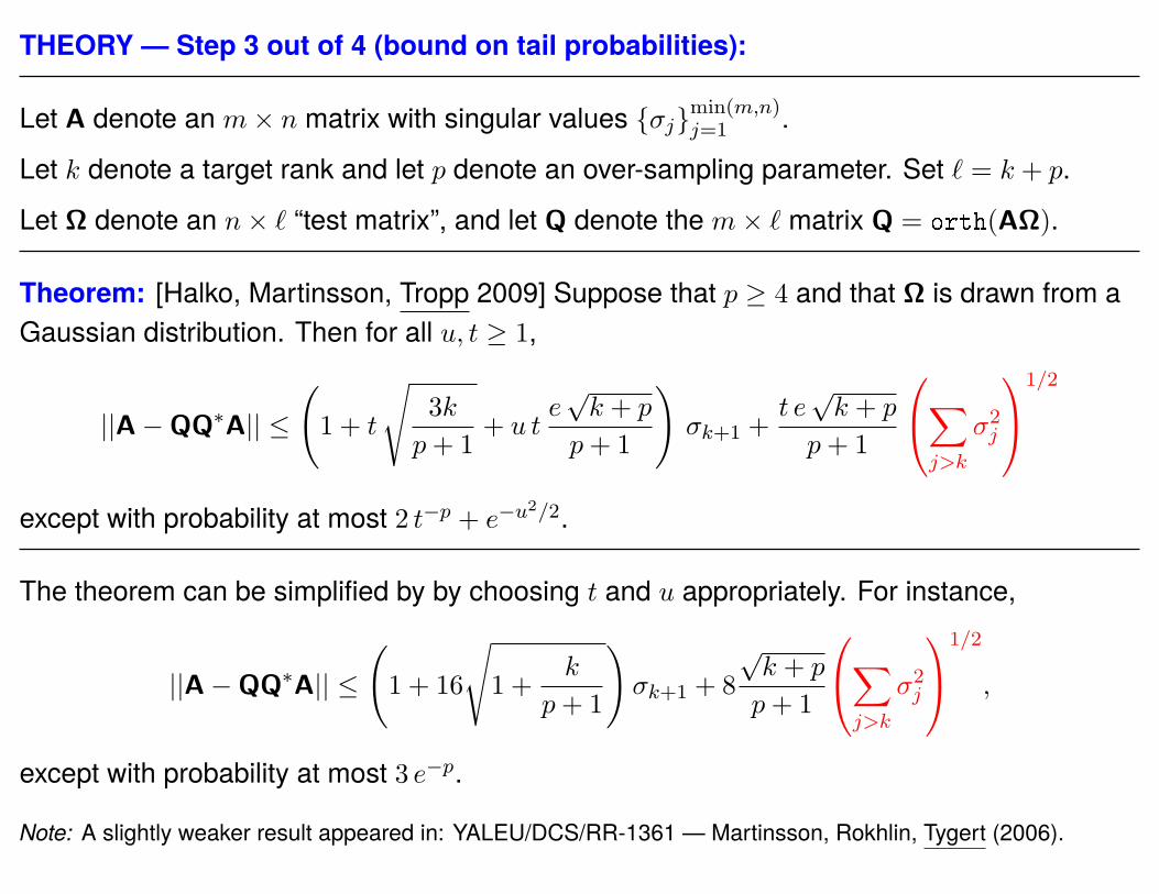
THEORY — Step 3 out of 4 (bound on tail probabilities):
Let A denote an m× n matrix with singular values σjmin(m,n)j=1 .
Let k denote a target rank and let p denote an over-sampling parameter. Set ℓ = k + p.
Let Ω denote an n× ℓ “test matrix”, and let Q denote the m× ℓ matrix Q = orth(AΩ).
Theorem: [Halko, Martinsson, Tropp 2009] Suppose that p ≥ 4 and that Ω is drawn from aGaussian distribution. Then for all u, t ≥ 1,
||A−QQ∗A|| ≤
(1 + t
√3k
p+ 1+ u t
e√k + p
p+ 1
)σk+1 +
t e√k + p
p+ 1
∑j>k
σ2j
1/2
except with probability at most 2 t−p + e−u2/2.
The theorem can be simplified by by choosing t and u appropriately. For instance,
||A−QQ∗A|| ≤
(1 + 16
√1 +
k
p+ 1
)σk+1 + 8
√k + p
p+ 1
∑j>k
σ2j
1/2
,
except with probability at most 3 e−p.
Note: A slightly weaker result appeared in: YALEU/DCS/RR-1361 — Martinsson, Rokhlin, Tygert (2006).

THEORY — Step 3 out of 4 (bound on tail probabilities):
Let A denote an m× n matrix with singular values σjmin(m,n)j=1 .
Let k denote a target rank and let p denote an over-sampling parameter. Set ℓ = k + p.
Let Ω denote an n× ℓ “test matrix”, and let Q denote the m× ℓ matrix Q = orth(AΩ).
Theorem: [Halko, Martinsson, Tropp 2009] Suppose that p ≥ 4 and that Ω is drawn from aGaussian distribution. Then for all u, t ≥ 1,
||A−QQ∗A|| ≤
(1 + t
√3k
p+ 1+ u t
e√k + p
p+ 1
)σk+1 +
t e√k + p
p+ 1
∑j>k
σ2j
1/2
except with probability at most 2 t−p + e−u2/2.
The theorem can be simplified by by choosing t and u appropriately. For instance,
||A−QQ∗A|| ≤(1 + 6
√(k + p) · p log p
)σk+1 + 3
√k + p
∑j>k
σ2j
1/2
,
except with probability at most 3 p−p.
Note: A slightly weaker result appeared in: YALEU/DCS/RR-1361 — Martinsson, Rokhlin, Tygert (2006).
THEORY — Step 4 out of 4 — comments on the case where Ω is an SRFT:
Let A denote an m× n matrix with singular values σjmin(m,n)j=1 .
Let k denote a target rank and let p denote an over-sampling parameter. Set ℓ = k + p.
Let Ω denote an n× ℓ “test matrix”, and let Q denote the m× ℓ matrix Q = orth(AΩ).
The current error analysis is disappointing:
• Failure probability decays very slowly with p (and depends on k).
• The number ℓ of samples required satisfies ℓ ∼ k log(k).This is sharp, there is a “coupon collection” type problem.
But, happily, the practical observed behavior of the method is excellent.In all actual applications we have tested, the SRFTs we have used perform essentially aswell as Gaussian test matrices. (Picking a slightly larger ℓ is advisable, say ℓ = 2k).
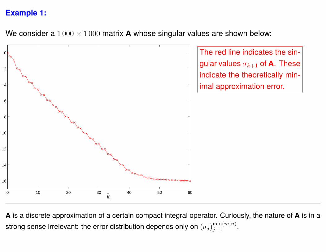
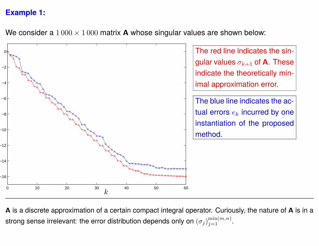
Example 1:
We consider a 1 000× 1 000 matrix A whose singular values are shown below:
0 10 20 30 40 50 60
−16
−14
−12
−10
−8
−6
−4
−2
0
k
log10(σ
k+1)
log10(e
k)
The red line indicates the sin-gular values σk+1 of A. Theseindicate the theoretically min-imal approximation error.
The blue line indicates the ac-tual errors ek incurred by oneinstantiation of the proposedmethod.
A is a discrete approximation of a certain compact integral operator. Curiously, the nature of A is in astrong sense irrelevant: the error distribution depends only on (σj)
min(m,n)j=1 .
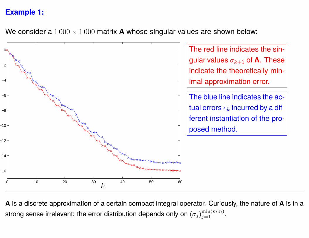
Example 1:
We consider a 1 000× 1 000 matrix A whose singular values are shown below:
0 10 20 30 40 50 60
−16
−14
−12
−10
−8
−6
−4
−2
0
k
log10(σ
k+1)
log10(e
k)
The red line indicates the sin-gular values σk+1 of A. Theseindicate the theoretically min-imal approximation error.
The blue line indicates the ac-tual errors ek incurred by a dif-ferent instantiation of the pro-posed method.
A is a discrete approximation of a certain compact integral operator. Curiously, the nature of A is in astrong sense irrelevant: the error distribution depends only on (σj)
min(m,n)j=1 .

Example 1:
We consider a 1 000× 1 000 matrix A whose singular values are shown below:
0 10 20 30 40 50 60
−16
−14
−12
−10
−8
−6
−4
−2
0
k
log10(σ
k+1)
log10(e
k)
The red line indicates the sin-gular values σk+1 of A. Theseindicate the theoretically min-imal approximation error.
The blue lines indicate the ac-tual errors ek incurred by 10different instantiations of theproposed method.
A is a discrete approximation of a certain compact integral operator. Curiously, the nature of A is in astrong sense irrelevant: the error distribution depends only on (σj)
min(m,n)j=1 .

Example 2:
The matrix A being analyzed is a 9025× 9025 matrix arising in a diffusion geometryapproach to image processing.
To be precise, A is a graph Laplacian on the manifold of 3× 3 patches.
!!!!!!
x )l
p(x )j
675872695376907452
p(x )i=
p(x )k
!!!!!!
!!!!!!
!!!!
!!!!!!
!!!!
!!!!
!!!!
!!!!!!
!!!!!!
!!!!!!
!!!
!!!!!!
!!!!!!
!!!
!!!!!!
!!!
!!!!!!
!!!
p(
!!!!
!!!!
!!!!!!
!!!!!!
!!!!!!
!!!!!!
!!!!!!
!!!!!!
!!!!
!!!!
!!!!
!!!!
!!!!!!
l
i
j
k
Joint work with François Meyer of the University of Colorado at Boulder.
0 20 40 60 80 1000
0.1
0.2
0.3
0.4
0.5
0.6
0.7
0.8
0.9
1
0 20 40 60 80 1000
0.1
0.2
0.3
0.4
0.5
0.6
0.7
0.8
0.9
1
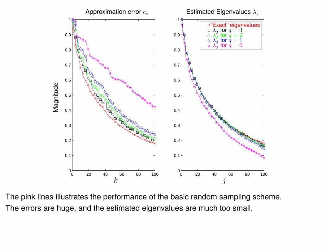
k j
Approximation error ek Estimated Eigenvalues λj
Mag
nitu
de
“Exact” eigenvaluesλj for q = 3λj for q = 2λj for q = 1λj for q = 0
The pink lines illustrates the performance of the basic random sampling scheme.The errors are huge, and the estimated eigenvalues are much too small.

Example 3: “Eigenfaces”
We next process a data base containing m = 7254 pictures of faces
Each image consists of n = 384× 256 = 98 304 gray scale pixels.
We center and scale the pixels in each image, and let the resulting values form a column ofa 98 304× 7 254 data matrix A.
The left singular vectors of A are the so called eigenfaces of the data base.

0 20 40 60 80 10010
0
101
102
0 20 40 60 80 10010
0
101
102Approximation error ek Estimated Singular Values σj
Mag
nitu
de
Minimal error (est)q = 0q = 1q = 2q = 3
k j
The pink lines illustrates the performance of the basic random sampling scheme.Again, the errors are huge, and the estimated eigenvalues are much too small.
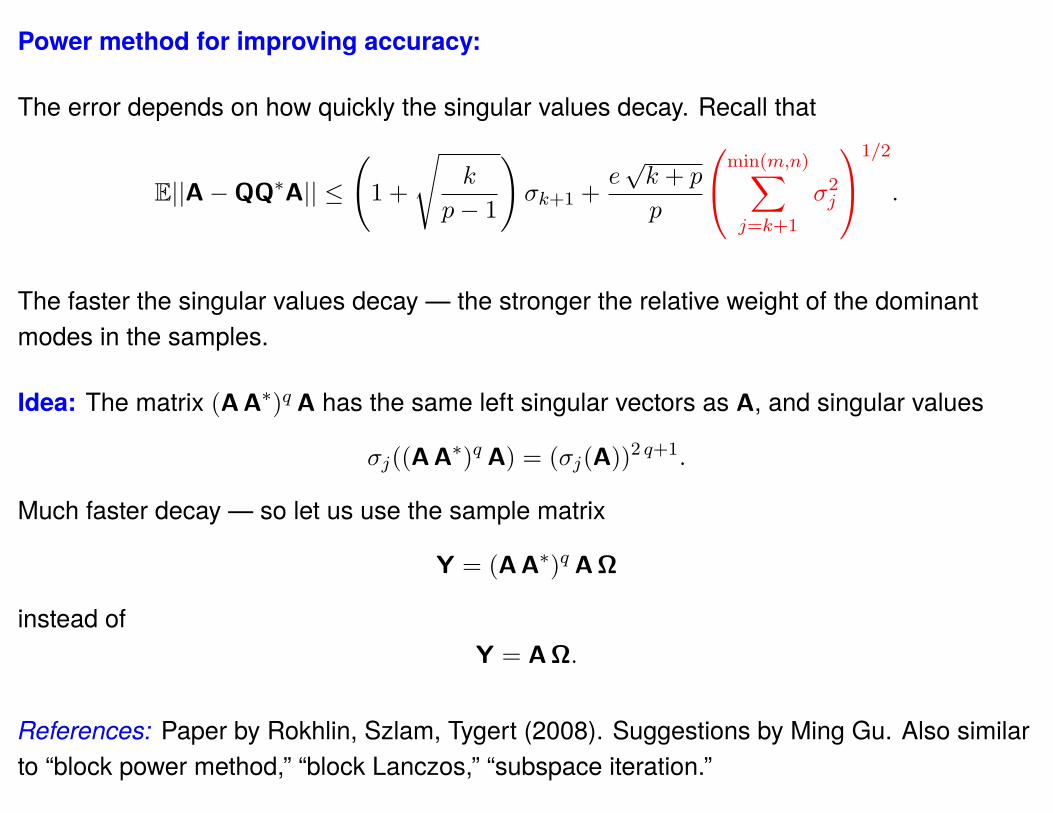
Power method for improving accuracy:
The error depends on how quickly the singular values decay. Recall that
E||A−QQ∗A|| ≤
(1 +
√k
p− 1
)σk+1 +
e√k + p
p
min(m,n)∑j=k+1
σ2j
1/2
.
The faster the singular values decay — the stronger the relative weight of the dominantmodes in the samples.
Idea: The matrix (AA∗)q A has the same left singular vectors as A, and singular values
σj((AA∗)q A) = (σj(A))2 q+1.
Much faster decay — so let us use the sample matrix
Y = (AA∗)q AΩ
instead ofY = AΩ.
References: Paper by Rokhlin, Szlam, Tygert (2008). Suggestions by Ming Gu. Also similarto “block power method,” “block Lanczos,” “subspace iteration.”
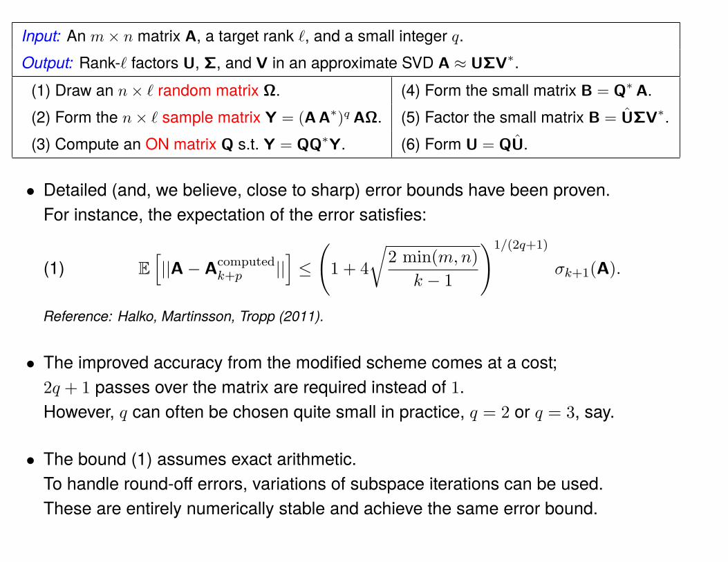
Input: An m× n matrix A, a target rank ℓ, and a small integer q.Output: Rank-ℓ factors U, Σ, and V in an approximate SVD A ≈ UΣV∗.
(1) Draw an n× ℓ random matrix Ω. (4) Form the small matrix B = Q∗ A.(2) Form the n× ℓ sample matrix Y = (AA∗)q AΩ. (5) Factor the small matrix B = UΣV∗.(3) Compute an ON matrix Q s.t. Y = QQ∗Y. (6) Form U = QU.
• Detailed (and, we believe, close to sharp) error bounds have been proven.For instance, the expectation of the error satisfies:
(1) E[||A− Acomputed
k+p ||]≤
(1 + 4
√2 min(m,n)
k − 1
)1/(2q+1)
σk+1(A).
Reference: Halko, Martinsson, Tropp (2011).
• The improved accuracy from the modified scheme comes at a cost;2q + 1 passes over the matrix are required instead of 1.However, q can often be chosen quite small in practice, q = 2 or q = 3, say.
• The bound (1) assumes exact arithmetic.To handle round-off errors, variations of subspace iterations can be used.These are entirely numerically stable and achieve the same error bound.

A numerically stable version of the “power method”:
Input: An m× n matrix A, a target rank ℓ, and a small integer q.Output: Rank-ℓ factors U, Σ, and V in an approximate SVD A ≈ UΣV∗.
Draw an n× ℓ Gaussian random matrix Ω.Set Q = orth(AΩ)
for i = 1, 2, . . . , q
W = orth(A∗Q)
Q = orth(AW)
end forB = Q∗A
[U, Σ, V] = svd(B)
U = QU.
Note: Algebraically, the method with orthogonalizations is identical to the “original” methodwhere Q = orth((AA∗)qAΩ).
Note: This is a classic subspace iteration.The novelty is the error analysis, and the finding that using a very small q is often fine.(In fact, our analysis allows q to be zero. . . )
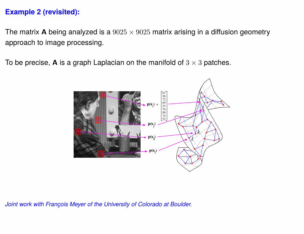
Example 2 (revisited):
The matrix A being analyzed is a 9025× 9025 matrix arising in a diffusion geometryapproach to image processing.
To be precise, A is a graph Laplacian on the manifold of 3× 3 patches.
!!!!!!
x )l
p(x )j
675872695376907452
p(x )i=
p(x )k
!!!!!!
!!!!!!
!!!!
!!!!!!
!!!!
!!!!
!!!!
!!!!!!
!!!!!!
!!!!!!
!!!
!!!!!!
!!!!!!
!!!
!!!!!!
!!!
!!!!!!
!!!
p(
!!!!
!!!!
!!!!!!
!!!!!!
!!!!!!
!!!!!!
!!!!!!
!!!!!!
!!!!
!!!!
!!!!
!!!!
!!!!!!
l
i
j
k
Joint work with François Meyer of the University of Colorado at Boulder.

0 20 40 60 80 1000
0.1
0.2
0.3
0.4
0.5
0.6
0.7
0.8
0.9
1
0 20 40 60 80 1000
0.1
0.2
0.3
0.4
0.5
0.6
0.7
0.8
0.9
1
k j
Approximation error ek Estimated Eigenvalues λj
Mag
nitu
de
“Exact” eigenvaluesλj for q = 3λj for q = 2λj for q = 1λj for q = 0
The pink lines illustrates the performance of the basic random sampling scheme.The errors are huge, and the estimated eigenvalues are much too small.

Example 3 (revisited): “Eigenfaces”
We next process a data base containing m = 7254 pictures of faces
Each image consists of n = 384× 256 = 98 304 gray scale pixels.
We center and scale the pixels in each image, and let the resulting values form a column ofa 98 304× 7 254 data matrix A.
The left singular vectors of A are the so called eigenfaces of the data base.

0 20 40 60 80 10010
0
101
102
0 20 40 60 80 10010
0
101
102Approximation error ek Estimated Singular Values σj
Mag
nitu
de
Minimal error (est)q = 0q = 1q = 2q = 3
k j
The pink lines illustrates the performance of the basic random sampling scheme.Again, the errors are huge, and the estimated eigenvalues are much too small.

Example of application: Nearest neighbor search in RD
Picture of a cluster of points in 2D.
Lay on quad-tree.
What do in higher dimensions?
Random projections followed by low-dimensional search.Several different projections are needed.
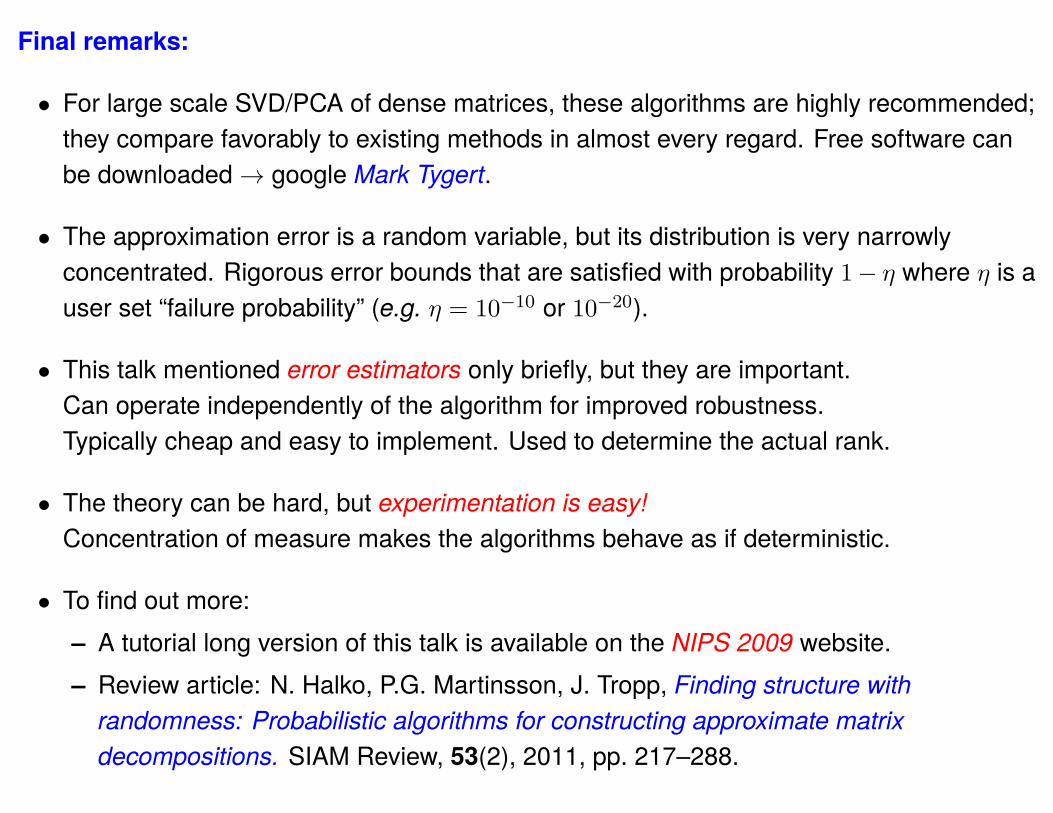
Final remarks:
• For large scale SVD/PCA of dense matrices, these algorithms are highly recommended;they compare favorably to existing methods in almost every regard. Free software canbe downloaded → google Mark Tygert.
• The approximation error is a random variable, but its distribution is very narrowlyconcentrated. Rigorous error bounds that are satisfied with probability 1− η where η is auser set “failure probability” (e.g. η = 10−10 or 10−20).
• This talk mentioned error estimators only briefly, but they are important.Can operate independently of the algorithm for improved robustness.Typically cheap and easy to implement. Used to determine the actual rank.
• The theory can be hard, but experimentation is easy!Concentration of measure makes the algorithms behave as if deterministic.
• To find out more:– A tutorial long version of this talk is available on the NIPS 2009 website.– Review article: N. Halko, P.G. Martinsson, J. Tropp, Finding structure with
randomness: Probabilistic algorithms for constructing approximate matrixdecompositions. SIAM Review, 53(2), 2011, pp. 217–288.

We note that the power method can be viewed as a hybrid between the “basic” randomizedmethod, and a Krylov subspace method:
Krylov method: Restrict A to the linear space
Vq(ω) = Span(Aω, A2ω, . . . , Aqω).
“Basic” randomized method: Restrict A to the linear space
Span(Aω1, Aω2, . . . , Aωℓ) = V1(ω1)× V1(ω2)× · · · × V1(ωℓ).
“Power” method: Restrict A to the linear space
Span(Aqω1, Aqω2, . . . , A
qωℓ).
Modified “power” method: Restrict A to the linear space
Vq(ω1)× Vq(ω2)× · · · × Vq(ωℓ).
This could be a promising area for further work.

The observation that a “thin” Gaussian random matrix to high probability is well-conditionedis at the heart of the celebrated Johnson-Lindenstrauss lemma:
Lemma: Let ε be a real number such that ε ∈ (0, 1), let n be a positive integer, and let k bean integer such that
(2) k ≥ 4
(ε2
2− ε3
3
)−1
log(n).
Then for any set V of n points in Rd, there is a map f : Rd → Rk such that
(3) (1− ε) ||u− v||2 ≤ ||f(u)− f(v)|| ≤ (1 + ε) ||u− v||2, ∀ u, v ∈ V.
Further, such a map can be found in randomized polynomial time.
It has been shown that an excellent choice of the map f is the linear map whose coefficientmatrix is a k × d matrix whose entries are i.i.d. Gaussian random variables (see,e.g. Dasgupta & Gupta (1999)).When k satisfies, (2), this map satisfies (3) with probability close to one.

The related Bourgain embedding theorem shows that such statements are not restricted toEuclidean space:
Theorem:. Every finite metric space (X, d) can be embedded into ℓ2 with distortion O(log n)
where n is the number of points in the space.
Again, random projections can be used as the maps.
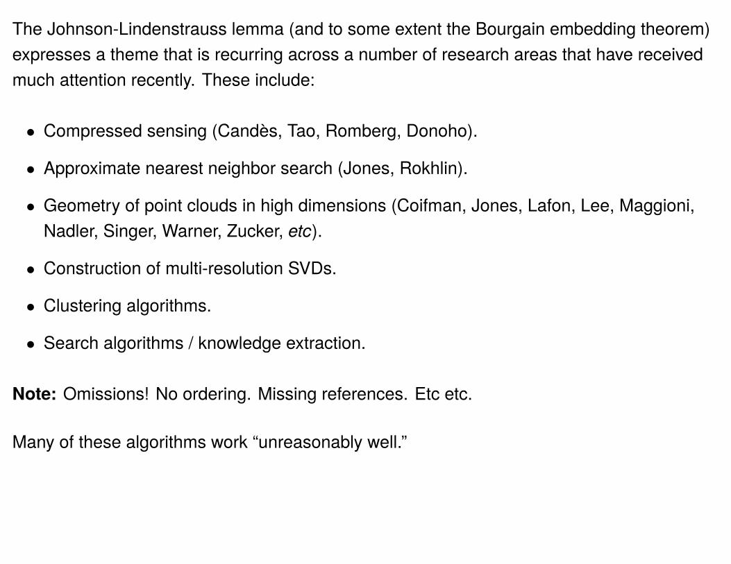
The Johnson-Lindenstrauss lemma (and to some extent the Bourgain embedding theorem)expresses a theme that is recurring across a number of research areas that have receivedmuch attention recently. These include:
• Compressed sensing (Candès, Tao, Romberg, Donoho).
• Approximate nearest neighbor search (Jones, Rokhlin).
• Geometry of point clouds in high dimensions (Coifman, Jones, Lafon, Lee, Maggioni,Nadler, Singer, Warner, Zucker, etc).
• Construction of multi-resolution SVDs.
• Clustering algorithms.
• Search algorithms / knowledge extraction.
Note: Omissions! No ordering. Missing references. Etc etc.
Many of these algorithms work “unreasonably well.”

The randomized algorithm presented here is close in spirit to randomized algorithms suchas:
• Randomized quick-sort.(With variations: computing the median / order statistics / etc.)
• Routing of data in distributed computing with unknown network topology.
• Rabin-Karp string matching / verifying equality of strings.
• Verifying polynomial identities.
Many of these algorithms are of the type that it is the running time that is stochastic. Thequality of the final output is excellent.
The randomized algorithm that is perhaps the best known within numerical analysis is MonteCarlo. This is somewhat lamentable given that MC is often a “last resort” type algorithmused when the curse of dimensionality hits — inaccurate results are tolerated simplybecause there are no alternatives.(These comments apply to the traditional “unreformed” version of MC — for manyapplications, more accurate versions have been developed.)

Observation: Mathematicians working on these problems often focus on minimizing thedistortion factor
1 + ε
1− ε
arising in the Johnson-Lindenstrauss bound:
(1− ε) ||u− v||2 ≤ ||f(u)− f(v)|| ≤ (1 + ε) ||u− v||2, ∀ u, v ∈ V.
In our environments, we do not need this constant to be particularly close to 1.It should just not be “large” — say less that 10 or some such.
This greatly reduces the number of random projections needed! Recall that in theJohnson-Lindenstrauss theorem:
number of samples required ∼ 1
ε2log(N).
Observation: Multiplication by a random unitary matrix reduces any matrix to its “general”form. All information about the singular vectors vanish. (The singular values remain thesame.)
This opens up the possibility for general pre-conditioners —counterexamples to various algorithms can be disregarded.
The feasibility has been demonstrated for the case of least squares solvers for very large,very over determined systems. (Work by Rokhlin & Tygert, Sarlós, . . . .)
Work on O(N2 (logN)2) solvers of general linear systems is under way.(Random pre-conditioning + iterative solver.)
May stable fast matrix inversion schemes for general matrices be possible?
Observation: Robustness with respect to the quality of the random numbers.
The assumption that the entries of the random matrix are i.i.d. normalized Gaussianssimplifies the analysis since this distribution is invariant under unitary maps.
In practice, however, one can use a low quality random number generator. The entries canbe uniformly distributed on [−1, 1], they be drawn from certain Bernouilli-type distributions,etc.
Remarkably, they can even have enough internal structure to allow fast methods formatrix-vector multiplications. For instance:
• Subsampled discrete Fourier transform.
• Subsampled Walsh-Hadamard transform.
• Givens rotations by random angles acting on random indices.
This was exploited in “Algorithm 2” (and related work by Ailon and Chazelle).Our theoretical understanding of such problems is unsatisfactory.Numerical experiments perform far better than existing theory indicates.


![Linear Programming Algorithmsjeffe.cs.illinois.edu/teaching/algorithms/notes/I-simplex.pdf · I. Linear Programming Algorithms [Springer,2001],whichcanbefreelydownloaded(butnotlegallyprinted)fromthe](https://static.fdocuments.us/doc/165x107/5e86f2386ccbff1e3f76924f/linear-programming-i-linear-programming-algorithms-springer2001whichcanbefreelydownloadedbutnotlegallyprintedfromthe.jpg)
![Widely-Linear Precoding for Large-Scale MIMO with IQI ... · arXiv:1702.08703v1 [cs.IT] 28 Feb 2017 1 Widely-Linear Precoding for Large-Scale MIMO with IQI: Algorithms and Performance](https://static.fdocuments.us/doc/165x107/5b6d1e5e7f8b9a0b558c859d/widely-linear-precoding-for-large-scale-mimo-with-iqi-arxiv170208703v1.jpg)


