Random Forests: some methodological insights - arXiv · Centre de recherche INRIA Saclay –...

arX

iv:0

811.

3619

v1 [

stat

.ML]

21

Nov

200

8

appor t de r ech er ch e

ISS

N02

49-6

399

ISR

NIN

RIA

/RR

--67

29--

FR

+E

NG

Thème COG

INSTITUT NATIONAL DE RECHERCHE EN INFORMATIQUE ET EN AUTOMATIQUE

Random Forests: some methodological insights

Robin Genuer — Jean-Michel Poggi — Christine Tuleau

N° 6729

Novembre 2008

http://arXiv.org/abs/0811.3619v1

Centre de recherche INRIA Saclay – Île-de-FranceParc Orsay Université

4, rue Jacques Monod, 91893 ORSAY CedexTéléphone : +33 1 72 92 59 00

Random Forests: some methodological insights

Robin Genuer ∗, Jean-Michel Poggi† ∗ , Christine Tuleau ‡

Theme COG — Systemes cognitifsEquipes-Projets Select

Rapport de recherche n° 6729 — Novembre 2008 — 32 pages

Abstract: This paper examines from an experimental perspective randomforests, the increasingly used statistical method for classification and regres-sion problems introduced by Leo Breiman in 2001. It first aims at confirming,known but sparse, advice for using random forests and at proposing some com-plementary remarks for both standard problems as well as high dimensionalones for which the number of variables hugely exceeds the sample size. But themain contribution of this paper is twofold: to provide some insights about thebehavior of the variable importance index based on random forests and in addi-tion, to propose to investigate two classical issues of variable selection. The firstone is to find important variables for interpretation and the second one is morerestrictive and try to design a good prediction model. The strategy involves aranking of explanatory variables using the random forests score of importanceand a stepwise ascending variable introduction strategy.

Key-words: Random Forests, Regression, Classification, Variable

Importance, Variable Selection.

∗ Universite Paris-Sud, Mathematique, Bat. 425, 91405 Orsay, France† Universite Paris Descartes, France‡ Universite Nice Sophia-Antipolis, France

Forets aleatoires : remarques methodologiques

Resume : On s’interesse a la methode des forets aleatoires d’un point de vuemethodologique. Introduite par Leo Breiman en 2001, elle est desormais large-ment utilisee tant en classification qu’en regression avec un succes spectaculaire.On vise tout d’abord a confirmer les resultats experimentaux, connus mais epars,quant au choix des parametres de la methode, tant pour les problemes dits ”stan-dards” que pour ceux dits de ”grande dimension” (pour lesquels le nombre devariables est tres grand vis a vis du nombre d’observations). Mais la contributionprincipale de cet article est d’etudier le comportement du score d’importance desvariables base sur les forets aleatoires et d’examiner deux problemes classiquesde selection de variables. Le premier est de degager les variables importantes ades fins d’interpretation tandis que le second, plus restrictif, vise a se restreindrea un sous-ensemble suffisant pour la prediction. La strategie generale procedeen deux etapes : le classement des variables base sur les scores d’importancesuivi d’une procedure d’introduction ascendante sequentielle des variables.

Mots-cles : Forets aleatoires, Regression, Classification, Impor-

tance des Variables, Selection des Variables.

Random Forests: some methodological insights 3

1 Introduction

Random forests (RF henceforth) is a popular and very efficient algorithm, basedon model aggregation ideas, for both classification and regression problems, in-troduced by Breiman (2001) [8]. It belongs to the family of ensemble methods,appearing in machine learning at the end of nineties (see for example Dietterich(1999) [15] and (2000) [16]). Let us briefly recall the statistical framework byconsidering a learning set L = {(X1, Y1), . . . , (Xn, Yn)} made of n i.i.d. obser-vations of a random vector (X, Y ). Vector X = (X1, ..., Xp) contains predictorsor explanatory variables, say X ∈ R

p, and Y ∈ Y where Y is either a class labelor a numerical response. For classification problems, a classifier t is a mappingt : R

p → Y while for regression problems, we suppose that Y = s(X) + ε ands is the so-called regression function. For more background on statistical learn-ing, see Hastie et al. (2001) [24]. Random forests is a model building strategyproviding estimators of either the Bayes classifier or the regression function.

The principle of random forests is to combine many binary decision treesbuilt using several bootstrap samples coming from the learning sample L andchoosing randomly at each node a subset of explanatory variables X . Moreprecisely, with respect to the well-known CART model building strategy (seeBreiman et al. (1984) [6]) performing a growing step followed by a pruning one,two differences can be noted. First, at each node, a given number (denoted bymtry) of input variables are randomly chosen and the best split is calculatedonly within this subset. Second, no pruning step is performed so all the treesare maximal trees.

In addition to CART, another well-known related tree-based method mustbe mentioned: bagging (see Breiman (1996) [7]). Indeed random forests withmtry = p reduce simply to unpruned bagging. The associated R1 packagesare respectively randomForest (intensively used in the sequel of the paper),rpart and ipred for CART and bagging respectively (cited here for the sake ofcompleteness).

RF algorithm becomes more and more popular and appears to be very pow-erful in a lot of different applications (see for example Dıaz-Uriarte and Alvarezde Andres (2006) [14] for gene expression data analysis) even if it is not clearlyelucidated from a mathematical point of view (see the recent paper by Biauet al. (2008) [5] and Buhlmann, Yu (2002) [11] for bagging). Nevertheless,Breiman (2001) [8] sketches an explanation of the good performance of randomforests related to the good quality of each tree (at least from the bias point ofview) together with the small correlation among the trees of the forest, wherethe correlation between trees is defined as the ordinary correlation of predictionson so-called out-of-bag (OOB henceforth) samples. The OOB sample which isthe set of observations which are not used for building the current tree, is usedto estimate the prediction error and then to evaluate variable importance.

Tuning method parameters

It is now classical to distinguish two typical situations depending on n thenumber of observations, and p the number of variables: standard (for n >> p)and high dimensional (when n << p). The first question when someone tryto use practically random forests is to get information about sensible values

1see http://www.r-project.org/

RR n° 6729

4 Genuer et. al

for the two main parameters of the method. Essentially, the study carried outin the two papers [8] and [14] give interesting insights but Breiman focuses onstandard problems while Dıaz-Uriarte and Alvarez de Andres concentrate onhigh dimensional classification ones.

So the first objective of this paper is to give compact information aboutselected bench datasets and to examine again the choice of the method param-eters addressing more closely the different situations.

RF variable importance

The quantification of the variable importance (VI henceforth) is an impor-tant issue in many applied problems complementing variable selection by inter-pretation issues. In the linear regression framework it is examined for exampleby Gromping (2007) [22], making a distinction between various variance de-composition based indicators: ”dispersion importance”, ”level importance” or”theoretical importance” quantifying explained variance or changes in the re-sponse for a given change of each regressor. Various ways to define and computeusing R such indicators are available (see Gromping (2006) [23]).

In the random forests framework, the most widely used score of importanceof a given variable is the increasing in mean of the error of a tree (MSE forregression and misclassification rate for classification) in the forest when theobserved values of this variable are randomly permuted in the OOB samples.Often, such random forests VI is called permutation importance indices in op-position to total decrease of node impurity measures already introduced in theseminal book about CART by Breiman et al. (1984) [6].

Even if only little investigation is available about RF variable importance,some interesting facts are collected for classification problems. This index canbe based on the average loss of another criterion, like the Gini entropy used forgrowing classification trees. Let us cite two remarks. The first one is that the RFGini importance is not fair in favor of predictor variables with many categorieswhile the RF permutation importance is a more reliable indicator (see Strobl etal. (2007) [36]). So we restrict our attention to this last one. The second oneis that it seems that permutation importance overestimates the variable impor-tance of highly correlated variables and they propose a conditional variant (seeStrobl et al. (2008) [37]). Let us mention that, in this paper, we do not noticesuch phenomenon. For classification problems, Ben Ishak, Ghattas (2008) [4]and Dıaz-Uriarte, Alvarez de Andres (2006) [14] for example, use RF variableimportance and note that it is stable for correlated predictors, scale invariantand stable with respect to small perturbations of the learning sample. But thesepreliminary remarks need to be extended and the recent paper by Archer et al.(2008) [3], focusing more specifically on the VI topic, do not answer some cru-cial questions about the variable importance behavior: like the importance ofa group of variables or its behavior in presence of highly correlated variables.This one is the second goal of this paper.

Variable selection

Many variable selection procedures are based on the cooperation of variableimportance for ranking and model estimation to evaluate and compare a familyof models. Three types of variable selection methods are distinguished (see Ko-havi et al. (1997) [27] and Guyon et al. (2003) [20]): ”filter” for which the scoreof variable importance does not depend on a given model design method; ”wrap-

INRIA


per” which include the prediction performance in the score calculation; andfinally ”embedded” which intricate more closely variable selection and modelestimation.

For non-parametric models, only a small number of methods are available,especially for the classification case. Let us briefly mention some of them, whichare potentially competing tools. Of course we must firstly mention the wrappermethods based on VI coming from CART, see Breiman et al. (1984) [6] andof course, random forests, see Breiman (2001) [8]. Then some examples of em-bedded methods: Poggi, Tuleau (2006) [30] propose a method based on CARTscores and using stepwise ascending procedure with elimination step; Guyon etal. (2002) [19] (and Rakotomamonjy (2003) [32]), propose SVM-RFE, a methodbased on SVM scores and using descending elimination. More recently, BenIshak et al. (2008) [4] propose a stepwise variant while Park et al. (2007) [29]propose a ”LARS” type strategy (see Efron et al. (2004) [17] for classificationproblems.

Let us recall that two distinct objectives about variable selection can be iden-tified: (1) to find important variables highly related to the response variable forinterpretation purpose; (2) to find a small number of variables sufficient for agood prediction of the response variable. The key tool for task 1 is thresholdingvariable importance while the crucial point for task 2 is to combine variableranking and stepwise introduction of variables on a prediction model building.It could be ascending in order to avoid to select redundant variables or, for thecase n << p, descending first to reach a classical situation n ∼ p, and thenascending using the first strategy, see Fan, Lv (2008) [18]. We propose in thispaper, a two-steps procedure, the first one is common while the second one de-pends on the objective interpretation or prediction.

The paper is organized as follows. After this introduction, Section 2 focuseson random forests parameters. Section 3 proposes to study the behavior of theRF variable importance index. Section 4 investigates the two classical issues ofvariable selection using the random forests based score of importance. Section5 finally opens discussion about future work.

2 Selecting method parameters

2.1 Experimental framework

2.1.1 RF procedure

The R package about random forests is based on the the seminal contributionof Breiman and Cutler [10] and is described in Liaw, Wiener (2002) [28]. In thispaper, we focus on the randomForest procedure. The two main parameters aremtry, the number of input variables randomly chosen at each split and ntree,the number of trees in the forest2.

A third parameter, denoted by nodesize, allows to specify the minimumnumber of observations in a node. We retain the default value (1 for classificationand 5 for regression) of this parameter for all of our experimentations, since itis close to the maximal tree choice.

2In all the paper, mtry = m with m ∈ R stands for mtry = ⌊m⌋

RR n° 6729

6 Genuer et. al

2.1.2 OOB error

In this section, we concentrate on the prediction performance of RF focusing onout-of-bag (OOB) error (see [8]). We use this kind of prediction error estimatefor three reasons: the main is that we are mainly interested in comparing resultsinstead of assessing models, the second is that it gives fair estimation comparedto the usual alternative test set error even if it is considered as a little bitoptimistic and the last one, but not the least, is that it is a default outputof the procedure. To avoid unsignificant sampling effects, each OOB errors isactually the mean of OOB error over 10 runs.

2.1.3 Datasets

We have collected information about the data sets considered in this paper: thename, the name of the corresponding data structure (when different), n, p, thenumber of classes c in the multiclass case, a reference, a website or a package.The two next tables contain synthetic information while details are postponedin the Appendix. We distinguish standard and high dimensional situations and,in addition, the three problems: regression, 2-class classification and multiclassclassification.

Table 1 displays some information about standard problems datasets: forclassification at the top and for regression at the bottom.

Name Observations Variables ClassesIonosphere 351 34 2Diabetes 768 8 2Sonar 208 60 2Votes 435 16 2Ringnorm 200 20 2Threenorm 200 20 2Twonorm 200 20 2Glass 214 9 6Letters 20000 16 26Sat-images 6435 36 6Vehicle 846 18 4Vowel 990 10 11Waveform 200 21 3BostonHousing 506 13Ozone 366 12Servo 167 4Friedman1 300 10Friedman2 300 4Friedman3 300 4

Table 1: Standard problems: data sets for classification at the top, and forregression at the bottom

Table 2 displays high dimensional problems datasets: for classification at thetop and for regression at the bottom.

INRIA


Name Observations Variables ClassesAdenocarcinoma 76 9868 2Colon 62 2000 2Leukemia 38 3051 2Prostate 102 6033 2Brain 42 5597 5Breast 96 4869 3Lymphoma 62 4026 3Nci 61 6033 8Srbct 63 2308 4toys data 100 100 to 1000 2PAC 209 467Friedman1 100 100 to 1000Friedman2 100 100 to 1000Friedman3 100 100 to 1000

Table 2: High dimensional problems: data sets for classification at the top, andfor regression at the bottom

2.2 Regression

About regression problems, even if it seems at first inspection that the seminalpaper by Breiman [8] closes the debate about good advice, it remains thatthe experimental results are about a variant which is not implemented in theuniversally used R package. Moreover, except this reference, at our knowledge,no such a general paper is available, so we develop again the Breiman’s studyboth for real and simulated data corresponding to the case n >> p and weprovide some additional study on data corresponding to the case n << p (suchexamples typically come from chemometrics).

We observe that the default value of mtry proposed by the R package is notoptimal, and that there is no improvement by using random forests with respectto unpruned bagging (obtained for mtry = p).

2.2.1 Standard problems

Let us briefly examine standard (n >> p) regression datasets. In Figure 1 forreal ones and for simulated ones in Figure 2. Each plot gives for mtry = 1 top the OOB error for three different values of ntree = 100, 500 and 1000. Thevertical solid line indicates the value mtry = p/3, the default value proposed bythe R package for regression problems, the vertical dashed line being the valuemtry =

√p.

Three remarks can be formulated. First, the OOB error is maximal formtry = 1 and then decreases quickly (except for the ozone dataset, for reasonsnot clearly elucidated), then as soon as mtry >

√p, the error remains the same.

Second, the choice mtry =√

p gives always lower OOB error than mtry = p/3,and the gain can be important. So the default value proposed by the R packageseems to be often not optimal, especially when ⌊p/3⌋ = 1. Lastly, the defaultvalue ntree = 500 is convenient, but a much smaller one ntree = 100 leads tocomparable results.

RR n° 6729

8 Genuer et. al

2 4 6 8 10 12

10

12

14

16

18

mtryO

OB

Err

or

BostonHousing

ntree=1005001000

2 4 6 8 10 12

20

21

22

23

24

25

26

Ozone

1 1.5 2 2.5 3 3.5 4

20

25

30

35

40

45

Servo

Figure 1: Standard regression: 3 real data sets

2 4 6 8 107

8

9

10

11

12

mtry

OO

B E

rror

friedman1

ntree=1005001000

1 1.5 2 2.5 3 3.5 4

2.5

3

3.5

x 104 friedman2

1 1.5 2 2.5 3 3.5 4

0.026

0.027

0.028

0.029

0.03

0.031

0.032

0.033

friedman3

Figure 2: Standard regression: 3 simulated data sets

So, for standard (n >> p) regression problems, it seems that there is no im-provement by using random forests with respect to unpruned bagging (obtainedfor mtry = p).

2.2.2 High dimensional problems

Let us start with a simulated data set for the high dimensional case n << p. Thisexample is built by adding extra noisy variables (independent and uniformlydistributed on [0, 1]) to the Friedman1 model defined by:

Y = 10 sin(πX1X2) + 20(X3 − 0.5)2 + 10X4 + 5X5 + ǫ

INRIA


where X1, . . . , X5 are independent and uniformly distributed on [0, 1] and ǫ ∼N (0, 1). So we have 5 variables related to the response Y , the others beingnoise. We set n = 100 and let p vary.

100

101

102

14

15

16

17

18

19

20

21

22

mtry

OO

B E

rror

p=100

ntree=100

500

1000

100

101

102

16

17

18

19

20

21

22

p=200

100

101

102

18

19

20

21

22

23

p=500

100

101

102

103

19

19.5

20

20.5

21

21.5

22

22.5

23

23.5

p=1000

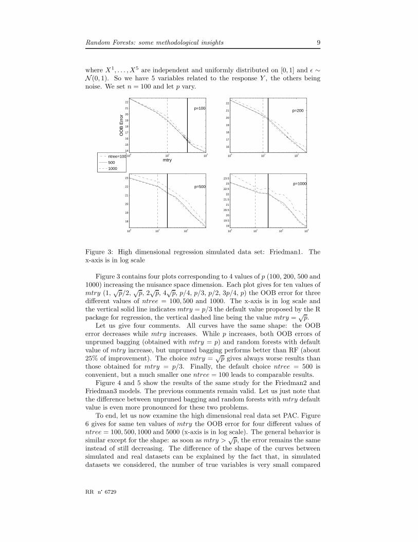
Figure 3: High dimensional regression simulated data set: Friedman1. Thex-axis is in log scale

Figure 3 contains four plots corresponding to 4 values of p (100, 200, 500 and1000) increasing the nuisance space dimension. Each plot gives for ten values ofmtry (1,

√p/2,

√p, 2

√p, 4

√p, p/4, p/3, p/2, 3p/4, p) the OOB error for three

different values of ntree = 100, 500 and 1000. The x-axis is in log scale andthe vertical solid line indicates mtry = p/3 the default value proposed by the Rpackage for regression, the vertical dashed line being the value mtry =

√p.

Let us give four comments. All curves have the same shape: the OOBerror decreases while mtry increases. While p increases, both OOB errors ofunpruned bagging (obtained with mtry = p) and random forests with defaultvalue of mtry increase, but unpruned bagging performs better than RF (about25% of improvement). The choice mtry =

√p gives always worse results than

those obtained for mtry = p/3. Finally, the default choice ntree = 500 isconvenient, but a much smaller one ntree = 100 leads to comparable results.

Figure 4 and 5 show the results of the same study for the Friedman2 andFriedman3 models. The previous comments remain valid. Let us just note thatthe difference between unpruned bagging and random forests with mtry defaultvalue is even more pronounced for these two problems.

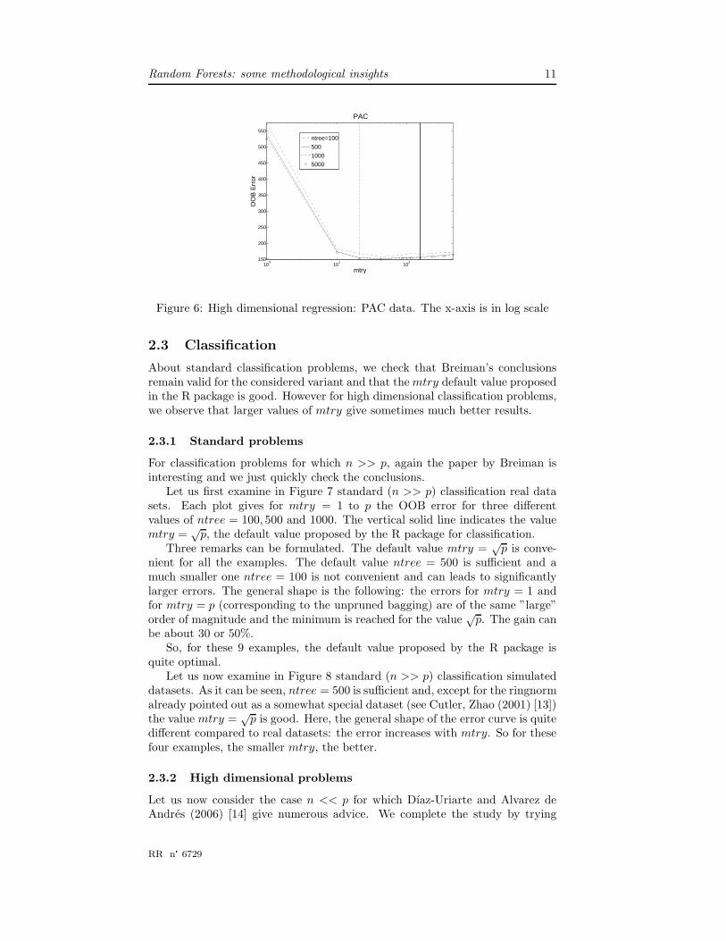
To end, let us now examine the high dimensional real data set PAC. Figure6 gives for same ten values of mtry the OOB error for four different values ofntree = 100, 500, 1000 and 5000 (x-axis is in log scale). The general behavior issimilar except for the shape: as soon as mtry >

√p, the error remains the same

instead of still decreasing. The difference of the shape of the curves betweensimulated and real datasets can be explained by the fact that, in simulateddatasets we considered, the number of true variables is very small compared

RR n° 6729

10 Genuer et. al

100

101

102

0.4

0.6

0.8

1

1.2

1.4

1.6

x 105

mtry

OO

B E

rror

p=100

ntree=100

500

1000

100

101

102

0.4

0.6

0.8

1

1.2

1.4

1.6

x 105

p=200

100

101

102

0.6

0.8

1

1.2

1.4

1.6

x 105

p=500

100

101

102

103

0.6

0.8

1

1.2

1.4

1.6

x 105

p=1000


100

101

102

0.07

0.08

0.09

0.1

0.11

0.12

mtry

OO

B E

rror

p=100

ntree=100

500

1000

100

101

102

0.07

0.08

0.09

0.1

0.11

0.12 p=200

100

101

102

0.08

0.085

0.09

0.095

0.1

0.105

0.11

0.115

0.12

0.125 p=500

100

101

102

103

0.08

0.085

0.09

0.095

0.1

0.105

0.11

0.115

0.12

0.125 p=1000


to the total number of variables. One may expect that in real datasets, theproportion of true variables is larger.

So, for high dimensional (n << p) regression problems, unpruned baggingseems to perform better than random forests and the difference can be large.

INRIA


100

101

102

150

200

250

300

350

400

450

500

550

mtry

OO

B E

rror

PAC

ntree=100

500

1000

5000

Figure 6: High dimensional regression: PAC data. The x-axis is in log scale

2.3 Classification

About standard classification problems, we check that Breiman’s conclusionsremain valid for the considered variant and that the mtry default value proposedin the R package is good. However for high dimensional classification problems,we observe that larger values of mtry give sometimes much better results.

2.3.1 Standard problems

For classification problems for which n >> p, again the paper by Breiman isinteresting and we just quickly check the conclusions.

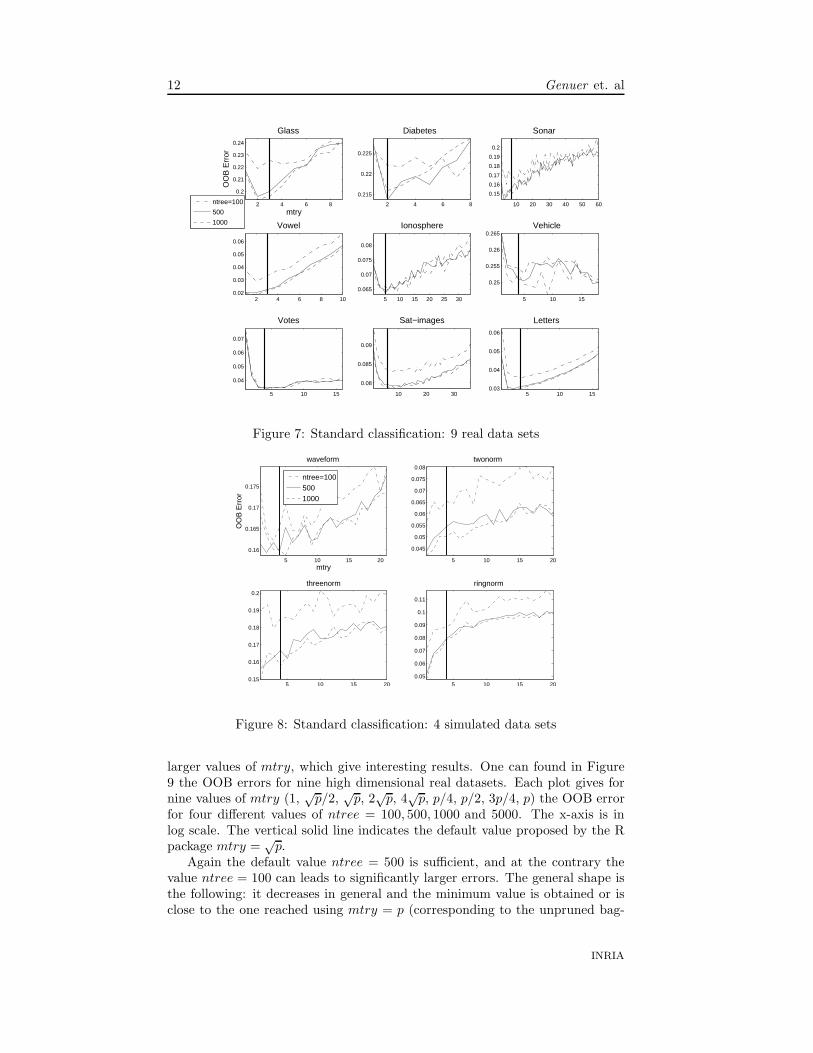
Let us first examine in Figure 7 standard (n >> p) classification real datasets. Each plot gives for mtry = 1 to p the OOB error for three differentvalues of ntree = 100, 500 and 1000. The vertical solid line indicates the valuemtry =

√p, the default value proposed by the R package for classification.

Three remarks can be formulated. The default value mtry =√

p is conve-nient for all the examples. The default value ntree = 500 is sufficient and amuch smaller one ntree = 100 is not convenient and can leads to significantlylarger errors. The general shape is the following: the errors for mtry = 1 andfor mtry = p (corresponding to the unpruned bagging) are of the same ”large”order of magnitude and the minimum is reached for the value

√p. The gain can

be about 30 or 50%.So, for these 9 examples, the default value proposed by the R package is

quite optimal.Let us now examine in Figure 8 standard (n >> p) classification simulated

datasets. As it can be seen, ntree = 500 is sufficient and, except for the ringnormalready pointed out as a somewhat special dataset (see Cutler, Zhao (2001) [13])the value mtry =

√p is good. Here, the general shape of the error curve is quite

different compared to real datasets: the error increases with mtry. So for thesefour examples, the smaller mtry, the better.

2.3.2 High dimensional problems

Let us now consider the case n << p for which Dıaz-Uriarte and Alvarez deAndres (2006) [14] give numerous advice. We complete the study by trying

RR n° 6729

12 Genuer et. al

2 4 6 8

0.2

0.21

0.22

0.23

0.24

mtry

OO

B E

rror

Glass

ntree=100

500

1000

2 4 6 8

0.215

0.22

0.225

Diabetes

10 20 30 40 50 60

0.15

0.16

0.17

0.18

0.19

0.2

Sonar

2 4 6 8 100.02

0.03

0.04

0.05

0.06

Vowel

5 10 15 20 25 30

0.065

0.07

0.075

0.08

Ionosphere

5 10 15

0.25

0.255

0.26

0.265Vehicle

5 10 15

0.04

0.05

0.06

0.07

Votes

10 20 30

0.08

0.085

0.09

Sat−images

5 10 150.03

0.04

0.05

0.06

Letters

Figure 7: Standard classification: 9 real data sets

5 10 15 20

0.16

0.165

0.17

0.175

mtry

OO

B E

rror

waveform

ntree=1005001000

5 10 15 20

0.045

0.05

0.055

0.06

0.065

0.07

0.075

0.08twonorm

5 10 15 200.15

0.16

0.17

0.18

0.19

0.2

threenorm

5 10 15 200.05

0.06

0.07

0.08

0.09

0.1

0.11

ringnorm

Figure 8: Standard classification: 4 simulated data sets

larger values of mtry, which give interesting results. One can found in Figure9 the OOB errors for nine high dimensional real datasets. Each plot gives fornine values of mtry (1,

√p/2,

√p, 2

√p, 4

√p, p/4, p/2, 3p/4, p) the OOB error

for four different values of ntree = 100, 500, 1000 and 5000. The x-axis is inlog scale. The vertical solid line indicates the default value proposed by the Rpackage mtry =

√p.

Again the default value ntree = 500 is sufficient, and at the contrary thevalue ntree = 100 can leads to significantly larger errors. The general shape isthe following: it decreases in general and the minimum value is obtained or isclose to the one reached using mtry = p (corresponding to the unpruned bag-

INRIA


100

102

0.155

0.16

0.165

0.17

0.175

mtry

OO

B E

rror

adenocarcinoma

ntree=100

500

1000

5000

100

102

0.2

0.25

0.3

0.35

brain

100

102

0.38

0.4

0.42

0.44

0.46

0.48

breast.3.class

100

102

0.15

0.2

0.25

0.3

colon

100

102

0

0.05

0.1

0.15

0.2

leukemia

100

102

0

0.02

0.04

0.06

0.08

lymphoma

100

102

0.35

0.4

0.45

0.5

nci

100

102

0.05

0.1

0.15

0.2

0.25

prostate

100

102

0.05

0.1

0.15

0.2

srbct

Figure 9: High dimensional classification: 9 real data sets. The x-axis is in logscale

ging). The difference with standard problems is notable, the reason is that whenp is large, mtry must be sufficiently large in order to have a high probability tocapture important variables (that is variables highly related to the response) fordefining the splits of the RF. In addition, let us mention that the default valuemtry =

√p is still reasonable from the OOB error viewpoint but of course, since√

p is small with respect to p, it is a very attractive value from a computationalperspective (notice that the trees are not too deep since n is not too large).

Let us examine a simulated dataset for the case n << p, introduced byWeston et al. (2003) [39], called “toys data” in the sequel. It is an equiprobabletwo-class problem, Y ∈ {−1, 1}, with 6 true variables, the others being somenoise. This example is interesting since it constructs two near independentgroups of 3 significant variables (highly, moderately and weakly correlated withresponse Y ) and an additional group of noise variables, uncorrelated with Y .A forward reference to the plots on the left side of Figure 11 allow to see thevariable importance picture and to note that the importance of the variables 1to 3 is much higher than the one of variables 4 to 6. More precisely, the modelis defined through the conditional distribution of the X i for Y = y:� for 70% of data, X i ∼ yN (i, 1) for i = 1, 2, 3 and X i ∼ yN (0, 1) for

i = 4, 5, 6.� for the 30% left, X i ∼ yN (0, 1) for i = 1, 2, 3 and X i ∼ yN (i − 3, 1) fori = 4, 5, 6.� the other variables are noise, X i ∼ N (0, 1) for i = 7, . . . , p.

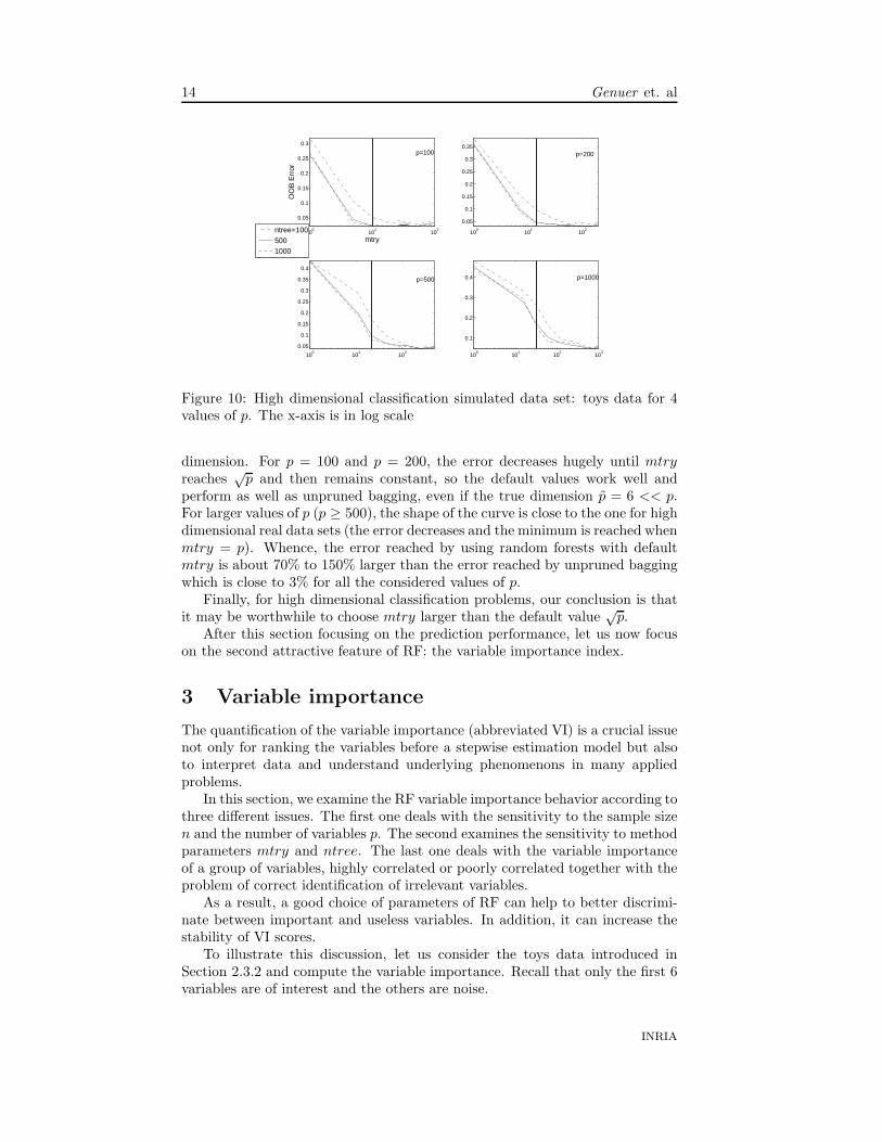
After simulation, obtained variables are standardized. Let us fix n = 100.The plots of Figure 10 are organized as previously, four values of p are

considered: 100, 200, 500 and 1000 corresponding to increasing nuisance space

RR n° 6729

14 Genuer et. al

100

101

102

0.05

0.1

0.15

0.2

0.25

0.3

mtry

OO

B E

rror

p=100

ntree=1005001000

100

101

102

0.05

0.1

0.15

0.2

0.25

0.3

0.35p=200

100

101

102

0.05

0.1

0.15

0.2

0.25

0.3

0.35

0.4

p=500

100

101

102

103

0.1

0.2

0.3

0.4 p=1000

Figure 10: High dimensional classification simulated data set: toys data for 4values of p. The x-axis is in log scale

dimension. For p = 100 and p = 200, the error decreases hugely until mtryreaches

√p and then remains constant, so the default values work well and

perform as well as unpruned bagging, even if the true dimension p = 6 << p.For larger values of p (p ≥ 500), the shape of the curve is close to the one for highdimensional real data sets (the error decreases and the minimum is reached whenmtry = p). Whence, the error reached by using random forests with defaultmtry is about 70% to 150% larger than the error reached by unpruned baggingwhich is close to 3% for all the considered values of p.

Finally, for high dimensional classification problems, our conclusion is thatit may be worthwhile to choose mtry larger than the default value

√p.

After this section focusing on the prediction performance, let us now focuson the second attractive feature of RF: the variable importance index.

3 Variable importance

The quantification of the variable importance (abbreviated VI) is a crucial issuenot only for ranking the variables before a stepwise estimation model but alsoto interpret data and understand underlying phenomenons in many appliedproblems.

In this section, we examine the RF variable importance behavior according tothree different issues. The first one deals with the sensitivity to the sample sizen and the number of variables p. The second examines the sensitivity to methodparameters mtry and ntree. The last one deals with the variable importanceof a group of variables, highly correlated or poorly correlated together with theproblem of correct identification of irrelevant variables.

As a result, a good choice of parameters of RF can help to better discrimi-nate between important and useless variables. In addition, it can increase thestability of VI scores.

To illustrate this discussion, let us consider the toys data introduced inSection 2.3.2 and compute the variable importance. Recall that only the first 6variables are of interest and the others are noise.

INRIA


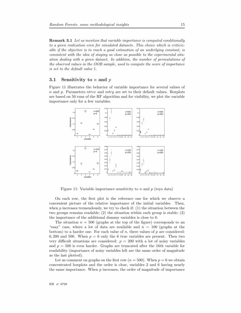
Remark 3.1 Let us mention that variable importance is computed conditionallyto a given realization even for simulated datasets. This choice which is criticiz-able if the objective is to reach a good estimation of an underlying constant, isconsistent with the idea of staying as close as possible to the experimental situ-ation dealing with a given dataset. In addition, the number of permutations ofthe observed values in the OOB sample, used to compute the score of importanceis set to the default value 1.

3.1 Sensitivity to n and p

Figure 11 illustrates the behavior of variable importance for several values ofn and p. Parameters ntree and mtry are set to their default values. Boxplotsare based on 50 runs of the RF algorithm and for visibility, we plot the variableimportance only for a few variables.

1 2 3 4 5 60

0.05

0.1

0.15

0.2

impo

rtan

ce

variable

n=500p=6

1 2 3 4 5 6 7 8 9 10 12 14 160

0.02

0.04

0.06

0.08

0.1

0.12

n=500p=200

1 2 3 4 5 6 7 8 9 10 12 14 160

0.02

0.04

0.06

0.08

0.1

0.12

n=500p=500

1 2 3 4 5 60

0.05

0.1

0.15

0.2

impo

rtan

ce

variable

n=100p=6

n=100p=200

1 2 3 4 5 6 7 8 9 10 12 14 16

0

0.01

0.02

0.03

0.04

0.05

0.06

0.07

0.08

n=100p=200

1 2 3 4 5 6 7 8 9 10 12 14 16

0

0.01

0.02

0.03

0.04

0.05

0.06

0.07

0.08

n=100p=500

Figure 11: Variable importance sensitivity to n and p (toys data)

On each row, the first plot is the reference one for which we observe aconvenient picture of the relative importance of the initial variables. Then,when p increases tremendously, we try to check if: (1) the situation between thetwo groups remains readable; (2) the situation within each group is stable; (3)the importance of the additional dummy variables is close to 0.

The situation n = 500 (graphs at the top of the figure) corresponds to an“easy” case, where a lot of data are available and n = 100 (graphs at thebottom) to a harder one. For each value of n, three values of p are considered:6, 200 and 500. When p = 6 only the 6 true variables are present. Then twovery difficult situations are considered: p = 200 with a lot of noisy variablesand p = 500 is even harder. Graphs are truncated after the 16th variable forreadability (importance of noisy variables left are the same order of magnitudeas the last plotted).

Let us comment on graphs on the first row (n = 500). When p = 6 we obtainconcentrated boxplots and the order is clear, variables 2 and 6 having nearlythe same importance. When p increases, the order of magnitude of importance

RR n° 6729

16 Genuer et. al

decreases. The order within the two groups of variables (1, 2, 3 and 4, 5, 6)remains the same, while the overall order is modified (variable 6 is now lessimportant than variable 2). In addition, variable importance is more unstablefor huge values of p. But what is remarkable is that all noisy variables have azero VI. So one can easily recover variables of interest.

In the second row(n = 100), we note a greater instability since the number ofobservations is only moderate, but the variable ranking remains quite the same.What differs is that in the difficult situations (p = 200, 500) importance of somenoisy variables increases, and for example variable 4 cannot be highlighted fromnoise (even variable 5 in the bottom right graph). This is due to the decreasingbehavior of VI with p growing, coming from the fact that when p = 500 thealgorithm randomly choose only 22 variables at each split (with the mtry defaultvalue). The probability of choosing one of the 6 true variables is really smalland the less a variable is chosen, the less it can be considered as important.

In addition, let us remark that the variability of VI is large for true variableswith respect to useless ones. This remark can be used to build some kind oftest for VI (see Strobl et al. (2007) [36]) but of course ranking is better suitedfor variable selection.

We now study how this VI index behaves when changing values of the mainmethod parameters.

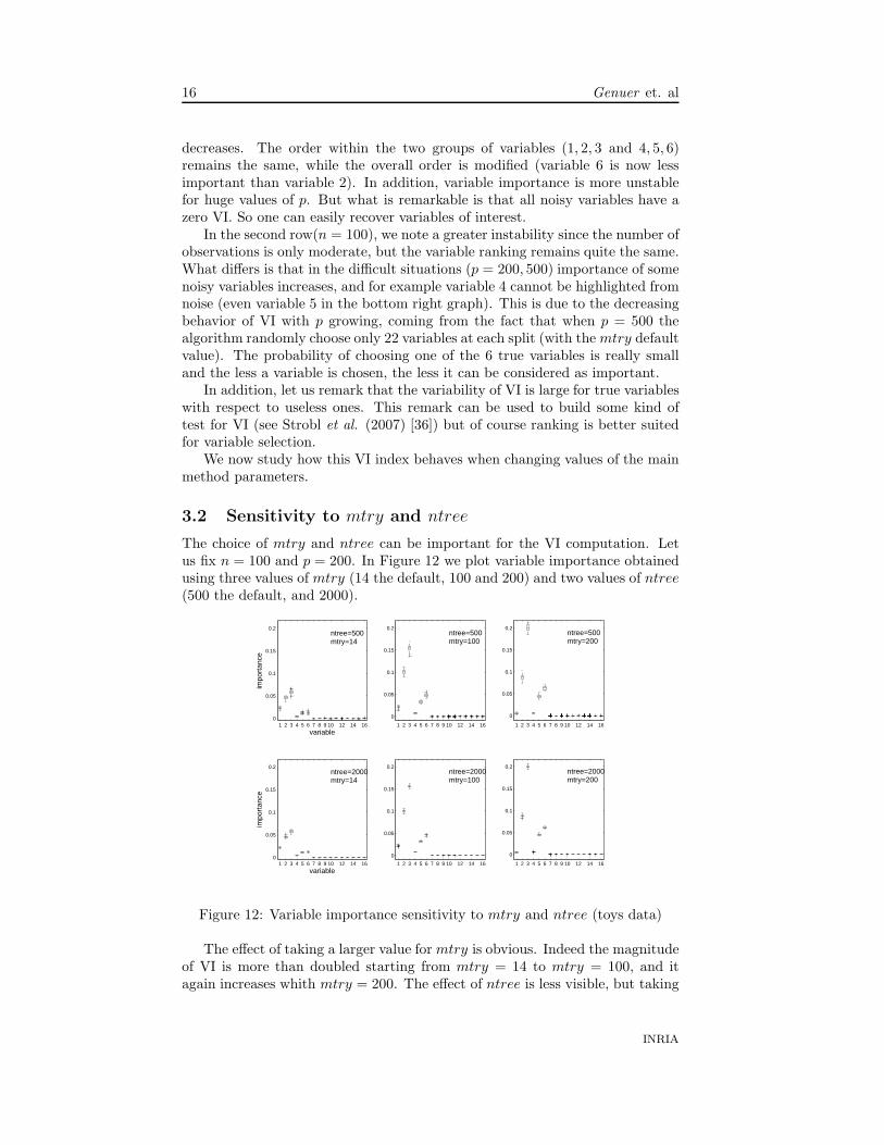
3.2 Sensitivity to mtry and ntree

The choice of mtry and ntree can be important for the VI computation. Letus fix n = 100 and p = 200. In Figure 12 we plot variable importance obtainedusing three values of mtry (14 the default, 100 and 200) and two values of ntree(500 the default, and 2000).

1 2 3 4 5 6 7 8 9 10 12 14 160

0.05

0.1

0.15

0.2

impo

rtan

ce

variable

ntree=500mtry=14

1 2 3 4 5 6 7 8 9 10 12 14 16

0

0.05

0.1

0.15

0.2ntree=500mtry=100

1 2 3 4 5 6 7 8 9 10 12 14 160

0.05

0.1

0.15

0.2

impo

rtan

ce

variable

ntree=2000mtry=14

1 2 3 4 5 6 7 8 9 10 12 14 16

0

0.05

0.1

0.15


1 2 3 4 5 6 7 8 9 10 12 14 16

0

0.05

0.1

0.15


1 2 3 4 5 6 7 8 9 10 12 14 16

0

0.05

0.1

0.15


Figure 12: Variable importance sensitivity to mtry and ntree (toys data)

The effect of taking a larger value for mtry is obvious. Indeed the magnitudeof VI is more than doubled starting from mtry = 14 to mtry = 100, and itagain increases whith mtry = 200. The effect of ntree is less visible, but taking

INRIA


ntree = 2000 leads to better stability. What is interesting in the bottom rightgraph is that we get the same order for all true variables in every run of theprocedure. In top left situation the mean OOB error rate is about 5% and inthe bottom right one it is 3%. The gain in error may not be considered as large,but what we get in VI is interesting.

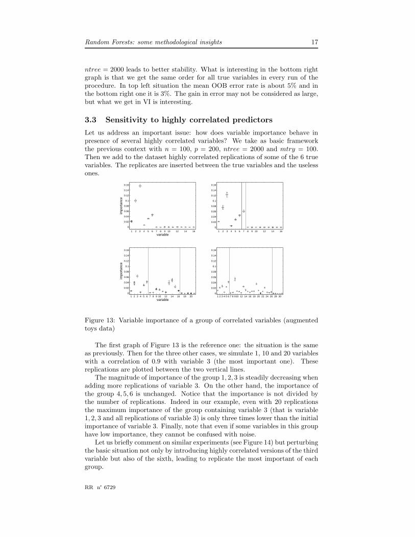
3.3 Sensitivity to highly correlated predictors

Let us address an important issue: how does variable importance behave inpresence of several highly correlated variables? We take as basic frameworkthe previous context with n = 100, p = 200, ntree = 2000 and mtry = 100.Then we add to the dataset highly correlated replications of some of the 6 truevariables. The replicates are inserted between the true variables and the uselessones.

1 2 3 4 5 6 7 8 9 10 12 14 16

0

0.02

0.04

0.06

0.08

0.1

0.12

0.14

0.16

impo

rtan

ce

variable1 2 3 4 5 6 7 8 9 10 12 14 16

0

0.02

0.04

0.06

0.08

0.1

0.12

0.14

0.16

1 2 3 4 5 6 7 8 9 10 12 14 16 18 200

0.02

0.04

0.06

0.08

0.1

0.12

0.14

0.16

impo

rtan

ce

variable1 2 3 4 5 6 7 8 910 12 14 16 18 20 22 24 26 28 30

0

0.02

0.04

0.06

0.08

0.1

0.12

0.14

0.16

Figure 13: Variable importance of a group of correlated variables (augmentedtoys data)

The first graph of Figure 13 is the reference one: the situation is the sameas previously. Then for the three other cases, we simulate 1, 10 and 20 variableswith a correlation of 0.9 with variable 3 (the most important one). Thesereplications are plotted between the two vertical lines.

The magnitude of importance of the group 1, 2, 3 is steadily decreasing whenadding more replications of variable 3. On the other hand, the importance ofthe group 4, 5, 6 is unchanged. Notice that the importance is not divided bythe number of replications. Indeed in our example, even with 20 replicationsthe maximum importance of the group containing variable 3 (that is variable1, 2, 3 and all replications of variable 3) is only three times lower than the initialimportance of variable 3. Finally, note that even if some variables in this grouphave low importance, they cannot be confused with noise.

Let us briefly comment on similar experiments (see Figure 14) but perturbingthe basic situation not only by introducing highly correlated versions of the thirdvariable but also of the sixth, leading to replicate the most important of eachgroup.

RR n° 6729

18 Genuer et. al

1 2 3 4 5 6 7 8 9 10 11 12 13 14 15 16

0

0.02

0.04

0.06

0.08

0.1

0.12

0.14

0.16

impo

rtan

cevariable

1 2 3 4 5 6 7 8 9 10 11 12 13 14 15 16

0

0.02

0.04

0.06

0.08

0.1

0.12

0.14

0.16

1 2 3 4 5 6 7 8 9 10 12 14 16 18 200

0.02

0.04

0.06

0.08

0.1

0.12

0.14

0.16

impo

rtan

ce

variable1 2 3 4 5 6 7 8 910 12 14 16 18 20 22 24 26 28 30 32

0

0.02

0.04

0.06

0.08

0.1

0.12

0.14

0.16

Figure 14: Variable importance of two groups of correlated variables (augmentedtoys data)

Again, the first graph is the reference one. Then we simulate 1, 5 and 10variables of correlation about 0.9 with variable 3 and the same with variable6. Replications of variable 3 are plotted between the first vertical line andthe dashed line, and replications of variable 6 between the dashed line and thesecond vertical line.

The magnitude of importance of each group (1, 2, 3 and 4, 5, 6 respectively)is steadily decreasing when adding more replications. The relative importancebetween the two groups is preserved. And the relative importance between thetwo groups of replications is of the same order than the one between the twoinitial groups.

3.4 Prostate data variable importance

To end this section, we illustrate the behavior of variable importance on a highdimensional real dataset: the microarray data called Prostate. The global pic-ture is the following: two variables hugely important, about twenty moderatelyimportant variables and the others of small importance. So, more precisely Fig-ure 15 compares VI obtained for parameters set to their default values (graphsof the left column) and those obtained for ntree = 2000 and mtry = p/3 (graphsof the right column).

Let us comment on Figure 15. For the two most important variables (firstrow), the magnitude of importance obtained with ntree = 2000 and mtry = p/3is much larger than to the one obtained with default values. In the second row,the increase of magnitude is still noticeable from the third to the 9th mostimportant variables and from the 10th to the 20th most important variables,VI is quite the same for the two parameter choices. In the third row, we get VIcloser to zero for the variables with ntree = 2000 and mtry = p/3 than withdefault values. In addition, note that for the less important variables, boxplotsare larger for default values, especially for unimportant variables (from the 200thto the 250th).

INRIA


1 20

0.02

0.04

0.06

0.08

0.1

variable

impo

rtan

ce

1 20

0.02

0.04

0.06

0.08

0.1

3 4 5 6 7 8 9 10 11 12 13 14 15 16 17 18 19 200

5

10

15x 10

−3

impo

rtan

ce

variable3 4 5 6 7 8 9 10 11 12 13 14 15 16 17 18 19 20

0

5

10

15x 10

−3

200 210 220 230 240 250

−5

0

5

10

x 10−4

impo

rtan

ce

variable200 210 220 230 240 250

−5

0

5

10

x 10−4

Figure 15: Variable importance for Prostate data (using ntree = 2000 andmtry = p/3, on the right and using default values on the left)

4 Variable selection

4.1 Procedure

4.1.1 Principle

We distinguish two variable selection objectives:

1. to find important variables highly related to the response variable forinterpretation purpose;

2. to find a small number of variables sufficient to a good prediction of theresponse variable.

The first is to magnify all the important variables, even with high redundancy,for interpretation purpose and the second is to find a sufficient parsimonious setof important variables for prediction.

Two earlier works must be cited: Dıaz-Uriarte, Alvarez de Andres (2006)[14] and Ben Ishak, Ghattas (2008) [4].

Dıaz-Uriarte, Alvarez de Andres propose a strategy based on recursive elim-ination of variables. More precisely, they first compute RF variable importance.Then, at each step, they eliminate the 20% of the variables having the smallestimportance and build a new forest with the remaining variables. They finallyselect the set of variables leading to the smallest OOB error rate. The propor-tion of variables to eliminate is an arbitrary parameter of their method and doesnot depend on the data.

RR n° 6729

20 Genuer et. al

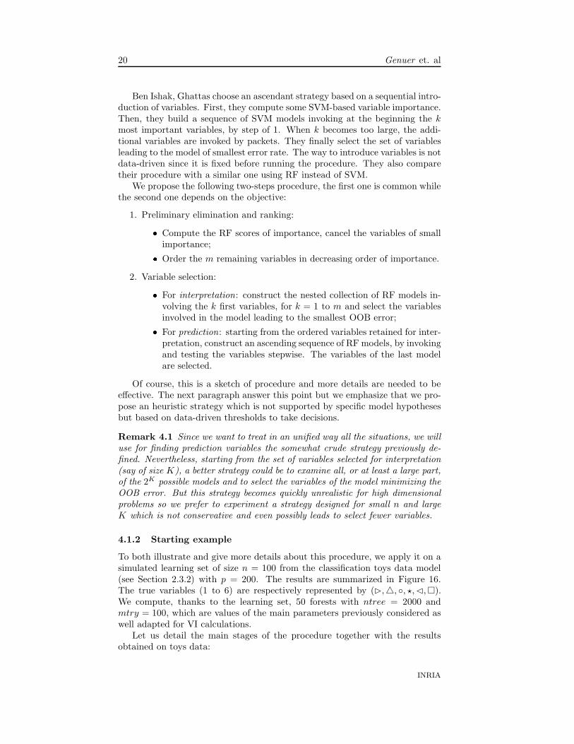
Ben Ishak, Ghattas choose an ascendant strategy based on a sequential intro-duction of variables. First, they compute some SVM-based variable importance.Then, they build a sequence of SVM models invoking at the beginning the kmost important variables, by step of 1. When k becomes too large, the addi-tional variables are invoked by packets. They finally select the set of variablesleading to the model of smallest error rate. The way to introduce variables is notdata-driven since it is fixed before running the procedure. They also comparetheir procedure with a similar one using RF instead of SVM.

We propose the following two-steps procedure, the first one is common whilethe second one depends on the objective:

1. Preliminary elimination and ranking:� Compute the RF scores of importance, cancel the variables of smallimportance;� Order the m remaining variables in decreasing order of importance.

2. Variable selection:� For interpretation: construct the nested collection of RF models in-volving the k first variables, for k = 1 to m and select the variablesinvolved in the model leading to the smallest OOB error;� For prediction: starting from the ordered variables retained for inter-pretation, construct an ascending sequence of RF models, by invokingand testing the variables stepwise. The variables of the last modelare selected.

Of course, this is a sketch of procedure and more details are needed to beeffective. The next paragraph answer this point but we emphasize that we pro-pose an heuristic strategy which is not supported by specific model hypothesesbut based on data-driven thresholds to take decisions.

Remark 4.1 Since we want to treat in an unified way all the situations, we willuse for finding prediction variables the somewhat crude strategy previously de-fined. Nevertheless, starting from the set of variables selected for interpretation(say of size K), a better strategy could be to examine all, or at least a large part,of the 2K possible models and to select the variables of the model minimizing theOOB error. But this strategy becomes quickly unrealistic for high dimensionalproblems so we prefer to experiment a strategy designed for small n and largeK which is not conservative and even possibly leads to select fewer variables.

4.1.2 Starting example

To both illustrate and give more details about this procedure, we apply it on asimulated learning set of size n = 100 from the classification toys data model(see Section 2.3.2) with p = 200. The results are summarized in Figure 16.The true variables (1 to 6) are respectively represented by (�,△, ◦, ⋆, �, �).We compute, thanks to the learning set, 50 forests with ntree = 2000 andmtry = 100, which are values of the main parameters previously considered aswell adapted for VI calculations.

Let us detail the main stages of the procedure together with the resultsobtained on toys data:

INRIA


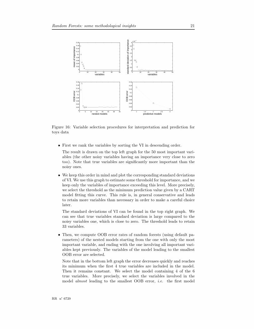
0 10 20 30 40 50

0

0.02

0.04

0.06

0.08

0.1

0.12

0.14

0.16

0.18

variablesm

ean

of im

port

ance

0 10 20 30 40 500

0.5

1

1.5

2

2.5

3

3.5

4x 10

−3

variablesstan

dard

dev

iatio

n of

impo

rtan

ce

0 5 10 15 20 25 30 350

0.02

0.04

0.06

0.08

0.1

0.12

0.14

0.16

0.18

nested models

OO

B e

rror

1 1.5 2 2.5 30

0.02

0.04

0.06

0.08

0.1

0.12

0.14

0.16

predictive models

OO

B e

rror

Figure 16: Variable selection procedures for interpretation and prediction fortoys data� First we rank the variables by sorting the VI in descending order.

The result is drawn on the top left graph for the 50 most important vari-ables (the other noisy variables having an importance very close to zerotoo). Note that true variables are significantly more important than thenoisy ones.� We keep this order in mind and plot the corresponding standard deviationsof VI. We use this graph to estimate some threshold for importance, and wekeep only the variables of importance exceeding this level. More precisely,we select the threshold as the minimum prediction value given by a CARTmodel fitting this curve. This rule is, in general conservative and leadsto retain more variables than necessary in order to make a careful choicelater.

The standard deviations of VI can be found in the top right graph. Wecan see that true variables standard deviation is large compared to thenoisy variables one, which is close to zero. The threshold leads to retain33 variables.� Then, we compute OOB error rates of random forests (using default pa-rameters) of the nested models starting from the one with only the mostimportant variable, and ending with the one involving all important vari-ables kept previously. The variables of the model leading to the smallestOOB error are selected.

Note that in the bottom left graph the error decreases quickly and reachesits minimum when the first 4 true variables are included in the model.Then it remains constant. We select the model containing 4 of the 6true variables. More precisely, we select the variables involved in themodel almost leading to the smallest OOB error, i.e. the first model

RR n° 6729

22 Genuer et. al

almost leading to the minimum. The actual minimum is reached with 24variables.

The expected behavior is non-decreasing as soon as all the ”true” variableshave been selected. It is then difficult to treat in a unified way nearlyconstant of or slightly increasing. In fact, we propose to use an heuristicrule similar to the 1 SE rule of Breiman et al. (1984) [6] used for selectionin the cost-complexity pruning procedure.� We perform a sequential variable introduction with testing: a variable isadded only if the error gain exceeds a threshold. The idea is that the errordecrease must be significantly greater than the average variation obtainedby adding noisy variables.

The bottom right graph shows the result of this step, the final modelfor prediction purpose involves only variables 3, 6 and 5. The thresholdis set to the mean of the absolute values of the first order differentiatederrors between the model with 5 variables (the first model after the onewe selected for interpretation, see the bottom left graph) and the last one.

It should be noted that if one wants to estimate the prediction error, sinceranking and selection are made on the same set of observations, of course an errorevaluation on a test set or using a cross validation scheme should be preferred.It is taken into account in the next section when our results are compared toothers.

To evaluate fairly the different prediction errors, we prefer here to simulatea test set of the same size than the learning set. The test error rate withall (200) variables is about 6% while the one with the 4 variables selected forinterpretation is about 4.5%, a little bit smaller. The model with predictionvariables 3, 6 and 5 reaches an error of 1%. Repeating the global procedure 10times on the same data always gave the same interpretation set of variables andthe same prediction set, in the same order.

4.1.3 Highly correlated variables

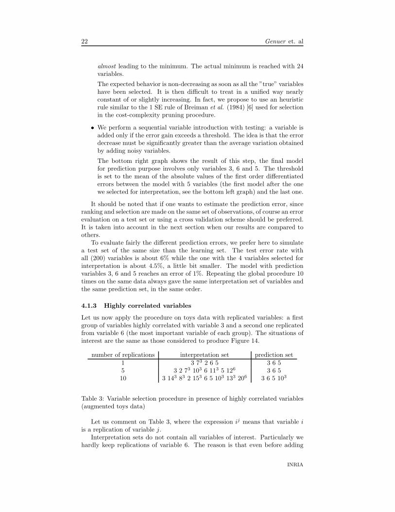
Let us now apply the procedure on toys data with replicated variables: a firstgroup of variables highly correlated with variable 3 and a second one replicatedfrom variable 6 (the most important variable of each group). The situations ofinterest are the same as those considered to produce Figure 14.

number of replications interpretation set prediction set1 3 73 2 6 5 3 6 55 3 2 73 103 6 113 5 126 3 6 510 3 143 83 2 153 6 5 103 133 206 3 6 5 103

Table 3: Variable selection procedure in presence of highly correlated variables(augmented toys data)

Let us comment on Table 3, where the expression ij means that variable iis a replication of variable j.

Interpretation sets do not contain all variables of interest. Particularly wehardly keep replications of variable 6. The reason is that even before adding

INRIA


noisy variables to the model the error rate of nested models do increase (orremain constant): when several highly correlated variables are added, the biasremains the same while the variance increases. However the prediction sets aresatisfactory: we always highlight variables 3 and 6 and at most one correlatedvariable with each of them.

Even if all the variables of interest do not appear in the interpretation set,they always appear in the first positions of our ranking according to importance.More precisely the 16 most important variables in the case of 5 replications are:(3 2 73 103 6 113 5 126 83 136 166 1 156 146 93 4), and the 26 most importantvariables in the case of 10 replications are: (3 143 83 2 153 6 5 103 133 206 216

113 123 186 1 246 73 266 236 163 256 226 176 196 4 93). Note that the order ofthe true variables (3 2 6 5 1 4) remains the same in all situations.

4.2 Classification

4.2.1 Prostate data

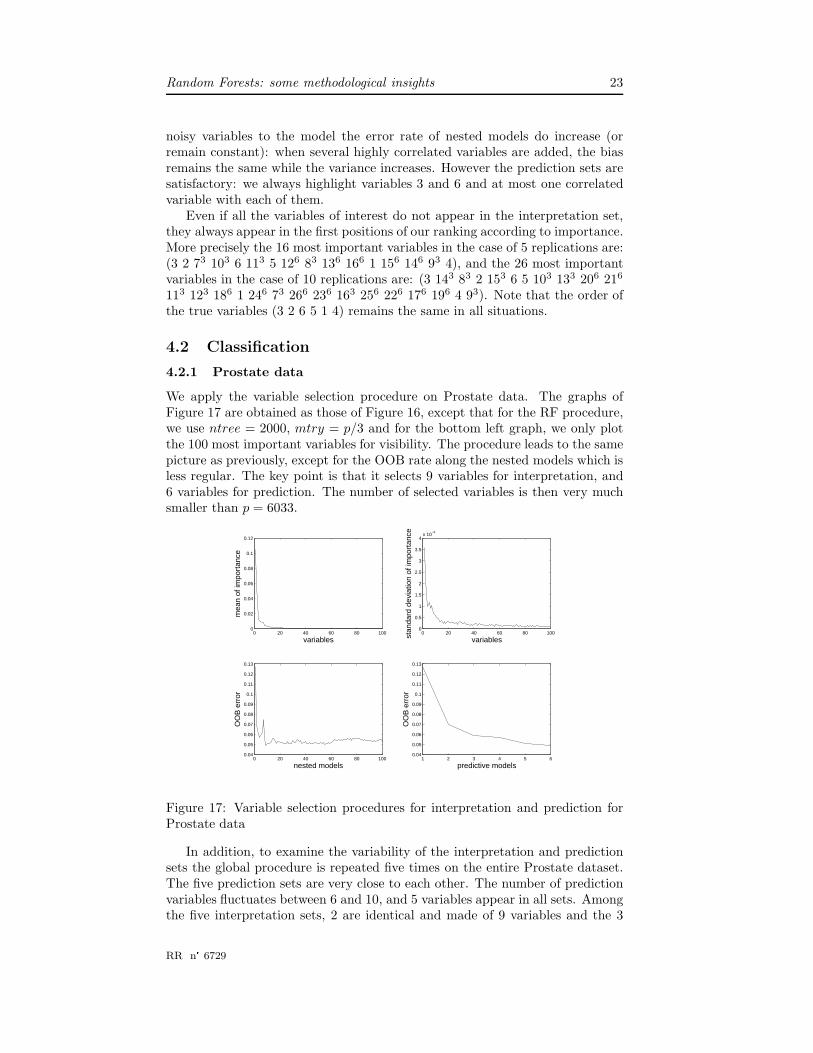
We apply the variable selection procedure on Prostate data. The graphs ofFigure 17 are obtained as those of Figure 16, except that for the RF procedure,we use ntree = 2000, mtry = p/3 and for the bottom left graph, we only plotthe 100 most important variables for visibility. The procedure leads to the samepicture as previously, except for the OOB rate along the nested models which isless regular. The key point is that it selects 9 variables for interpretation, and6 variables for prediction. The number of selected variables is then very muchsmaller than p = 6033.

0 20 40 60 80 1000

0.02

0.04

0.06

0.08

0.1

0.12

variables

mea

n of

impo

rtan

ce

0 20 40 60 80 1000

0.5

1

1.5

2

2.5

3

3.5

4x 10

−3

variablesstan

dard

dev

iatio

n of

impo

rtan

ce

1 2 3 4 5 60.04

0.05

0.06

0.07

0.08

0.09

0.1

0.11

0.12

0.13

predictive models

OO

B e

rror

0 20 40 60 80 1000.04

0.05

0.06

0.07

0.08

0.09

0.1

0.11

0.12

0.13

nested models

OO

B e

rror

Figure 17: Variable selection procedures for interpretation and prediction forProstate data

In addition, to examine the variability of the interpretation and predictionsets the global procedure is repeated five times on the entire Prostate dataset.The five prediction sets are very close to each other. The number of predictionvariables fluctuates between 6 and 10, and 5 variables appear in all sets. Amongthe five interpretation sets, 2 are identical and made of 9 variables and the 3

RR n° 6729

24 Genuer et. al

other are made of 25 variables. The 9 variables of the smallest sets are presentin all sets and the biggest sets (of size 25) have 23 variables in common.

So, although the sets of variables are not identical for each run of the pro-cedure, they are not completely different. And in addition the most importantvariables are included in all sets of variables.

4.2.2 High dimensional classification

We apply the global variable selection procedure on high dimensional real datasetsstudied in Section 2.3.2, and we want to get an estimation of prediction errorrates. Since these datasets are of small size, we use a 5-fold cross-validation toestimate the error rate. So we split the sample in 5 stratified parts, each part issuccessively used as a test set, and the remaining of the data is used as a learn-ing set. Note that the set of variables selected vary from one fold to another.So, we give in Table 4 the misclassification error rate, given by the 5-fold cross-validation, for interpretation and prediction sets of variables respectively. Thenumber into brackets is the average number of selected variables. In addition,one can find the original error which stands for the misclassification rate givenby the 5-fold cross-validation achieved with random forests using all variables.This error is calculated using the same partition in 5 parts and again we usentree = 2000 and mtry = p/3 for all datasets.

Dataset interpretation prediction originalColon 0.16 (35) 0.20 (8) 0.14

Leukemia 0 (1) 0 (1) 0.02Lymphoma 0.08 (77) 0.09 (12) 0.10Prostate 0.085 (33) 0.075 (8) 0.07

Table 4: Variable selection procedure for four high dimensional real datasets.CV-error rate and into brackets the average number of selected variables

The number of interpretation variables is hugely smaller than p, at mosttens to be compared to thousands. The number of prediction variables is verysmall (always smaller than 12) and the reduction can be very important w.r.tthe interpretation set size. The errors for the two variable selection proceduresare of the same order of magnitude as the original error (but a little bit larger).

We compare these results with the results obtained by Ben Ishak and Ghattas(2008) (see tables 9 and 11 in [4]) which have compared their method with 5competitors (mentioned in the introduction) for classification problems on thesefour datasets. Error rates are comparable. With the prediction procedure, asalready noted in the introductory remark, we always select fewer variables thantheir procedures (except for their method GLMpath which select less than 3variables for all datasets).

4.3 Regression

4.3.1 A simulated dataset

We now apply the procedure to a simulated regression problem. We constructstarting from the Friedman1 model and adding noisy variables as in Section

INRIA


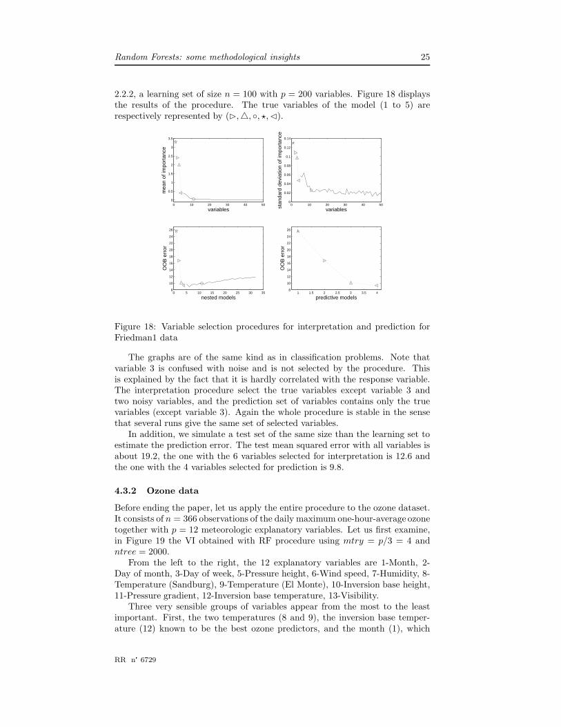
2.2.2, a learning set of size n = 100 with p = 200 variables. Figure 18 displaysthe results of the procedure. The true variables of the model (1 to 5) arerespectively represented by (�,△, ◦, ⋆, �).

0 10 20 30 40 500

0.5

1

1.5

2

2.5

3

3.5

variables

mea

n of

impo

rtan

ce

0 10 20 30 40 500

0.02

0.04

0.06

0.08

0.1

0.12

0.14

variablesstan

dard

dev

iatio

n of

impo

rtan

ce

0 5 10 15 20 25 30 358

10

12

14

16

18

20

22

24

26

nested models

OO

B e

rror

1 1.5 2 2.5 3 3.5 48

10

12

14

16

18

20

22

24

26

predictive models

OO

B e

rror

Figure 18: Variable selection procedures for interpretation and prediction forFriedman1 data

The graphs are of the same kind as in classification problems. Note thatvariable 3 is confused with noise and is not selected by the procedure. Thisis explained by the fact that it is hardly correlated with the response variable.The interpretation procedure select the true variables except variable 3 andtwo noisy variables, and the prediction set of variables contains only the truevariables (except variable 3). Again the whole procedure is stable in the sensethat several runs give the same set of selected variables.

In addition, we simulate a test set of the same size than the learning set toestimate the prediction error. The test mean squared error with all variables isabout 19.2, the one with the 6 variables selected for interpretation is 12.6 andthe one with the 4 variables selected for prediction is 9.8.

4.3.2 Ozone data

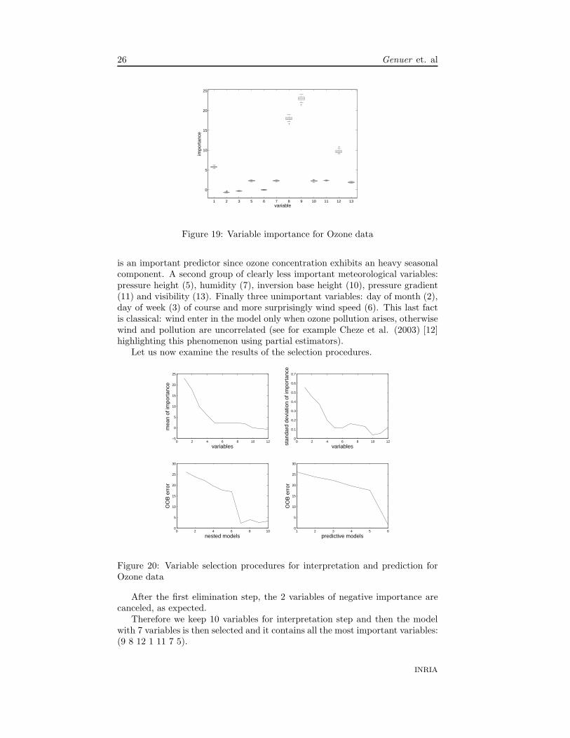
Before ending the paper, let us apply the entire procedure to the ozone dataset.It consists of n = 366 observations of the daily maximum one-hour-average ozonetogether with p = 12 meteorologic explanatory variables. Let us first examine,in Figure 19 the VI obtained with RF procedure using mtry = p/3 = 4 andntree = 2000.

From the left to the right, the 12 explanatory variables are 1-Month, 2-Day of month, 3-Day of week, 5-Pressure height, 6-Wind speed, 7-Humidity, 8-Temperature (Sandburg), 9-Temperature (El Monte), 10-Inversion base height,11-Pressure gradient, 12-Inversion base temperature, 13-Visibility.

Three very sensible groups of variables appear from the most to the leastimportant. First, the two temperatures (8 and 9), the inversion base temper-ature (12) known to be the best ozone predictors, and the month (1), which

RR n° 6729

26 Genuer et. al

1 2 3 5 6 7 8 9 10 11 12 13

0

5

10

15

20

25

impo

rtan

cevariable

Figure 19: Variable importance for Ozone data

is an important predictor since ozone concentration exhibits an heavy seasonalcomponent. A second group of clearly less important meteorological variables:pressure height (5), humidity (7), inversion base height (10), pressure gradient(11) and visibility (13). Finally three unimportant variables: day of month (2),day of week (3) of course and more surprisingly wind speed (6). This last factis classical: wind enter in the model only when ozone pollution arises, otherwisewind and pollution are uncorrelated (see for example Cheze et al. (2003) [12]highlighting this phenomenon using partial estimators).

Let us now examine the results of the selection procedures.

0 2 4 6 8 10 12−5

0

5

10

15

20

25

variables

mea

n of

impo

rtan

ce

0 2 4 6 8 10 120

0.1

0.2

0.3

0.4

0.5

0.6

0.7

variablesstan

dard

dev

iatio

n of

impo

rtan

ce

0 2 4 6 8 100

5

10

15

20

25

30

nested models

OO

B e

rror

1 2 3 4 5 60

5

10

15

20

25

30

predictive models

OO

B e

rror

Figure 20: Variable selection procedures for interpretation and prediction forOzone data

After the first elimination step, the 2 variables of negative importance arecanceled, as expected.

Therefore we keep 10 variables for interpretation step and then the modelwith 7 variables is then selected and it contains all the most important variables:(9 8 12 1 11 7 5).

INRIA


For the prediction procedure, the model is the same except one more variableis eliminated: humidity (7) .

In addition, when different values for mtry are considered, the most impor-tant 4 variables (9 8 12 1) highlighted by the VI index, are selected and appearin the same order. The variable 5 also always appears but another one canappear after of before.

5 Discussion

Of course, one of the main open issue about random forests is to elucidate froma mathematical point of view its exceptionally attractive performance. In fact,only a small number of references deal with this very difficult challenge and, inaddition to bagging theoretical examination by Bulmann and Yu (2002) [11],only purely random trees, a simple version of random forests, is considered.Purely random trees have been introduced by Cutler and Zhao (2001) [13] forclassification problems and then studied by Breiman (2004) [9], but the resultsare somewhat preliminary. More recently Biau et al. (2008) [5] obtained thefirst well stated consistency type results.

From a practical perspective, surprisingly, this simplified and essentially notdata-driven strategy seems to perform well, at least for prediction purpose (seeCutler and Zhao 2001 [13]) and, of course, can be handled theoretically ina easier way. Nevertheless, it should be interesting to check that the sameconclusions hold for variable importance and variable selection tasks.

In addition, it could be interesting to examine some variants of randomforests which, at the contrary, try to take into account more information. Letus give for example two ideas. The first is about pruning: why pruning is notused for individual trees? Of course, from the computational point of viewthe answer is obvious and for prediction performance, averaging eliminate thenegative effects of individual overfitting. But from the two other previouslymentioned statistical problems, prediction and variable selection, it remainsunclear. The second remark is about the random feature selection step. Themost widely used version of RF selects randomly mtry input variables accordingto the discrete uniform distribution. Two variants can be suggested: the first isto select random inputs according to a distribution coming from a preliminaryranking given by a pilot estimator; the second one is to adaptively update thisdistribution taking profit of the ranking based on the current forest which isthen more and more accurate.

These different future directions, both theoretical and practical, will be ad-dressed in the next step of the work.

6 Appendix

In the sequel, information about datasets retrieved from the R package mlbenchcan be found in the corresponding description file.

Standard problems, n >> p:� Binary classification

RR n° 6729

28 Genuer et. al

– Real data sets3* Ionosphere (n = 351, p = 34)* Diabetes, PimaIndiansDiabetes2 (n = 768, p = 8)* Sonar (n = 208, p = 60)* Votes, HouseVotes84 (n = 435, p = 16)

– Simulated data sets3* Ringnorm, mlbench.ringnorm (n = 200, p = 20)* Threenorm, mlbench.threenorm (n = 200, p = 20)* Twonorm, mlbench.twonorm (n = 200, p = 20)� Multiclass classification

– Real data sets3* Glass (n = 214, p = 9, c = 6)* Letters, LetterRecognition (n = 20000, p = 16, c = 26)* Sat-images, Satellite (n = 6435, p = 36, c = 6)* Vehicle (n = 846, p = 18, c = 4)* Vowel (n = 990, p = 10, c = 11)

– Simulated data sets3* Waveform, mlbench.waveform (n = 200, p = 21, c = 3)� Regression

– Real data sets3* BostonHousing (n = 506, p = 13)* Ozone (n = 366, p = 12)* Servo (n = 167, p = 4)

– Simulated data sets3* Friedman1, mlbench.friedman1 (n = 300, p = 10)* Friedman2, mlbench.friedman2 (n = 300, p = 4)* Friedman3, mlbench.friedman3 (n = 300, p = 4)

High dimensional problems, n << p:� Binary classification

– Real data sets4* Adenocarcinoma (n = 76, p = 9868), see Ramaswamy et al.(2003) [33]* Colon (n = 62, p = 2000), see Alon et al. (1999) [1]* Leukemia (n = 38, p = 3051): see Golub et al. (1999) [21]* Prostate (n = 102, p = 6033): see Singh et al. (2002) [35]

– Simulated data sets5

3from the R package mlbench

4see http://ligarto.org/rdiaz/Papers/rfVS/randomForestVarSel.html5see description in section 2.3.2

INRIA

Random Forests: some methodological insights 29* toys data (n = 100, 100 ≤ p ≤ 1000), see Weston et al. (2003)[39]� Multiclass classification

– Real data sets4* Brain (n = 42, p = 5597, c = 5), see Pomeroy et al. (2002) [31]* Breast, breast.3.class (n = 96, p = 4869, c = 3), see van’tVeer et al. (2002) [38]* Lymphoma (n = 62, p = 4026, c = 3), see Alizadeh (2000) [2]* Nci (n = 61, p = 6033, c = 8), see Ross et al. (2000) [34]* Srbct (n = 63, p = 2308, c = 4), see Khan et al. (2001) [26]� Regression

– Real data sets6* PAC (n = 209, p = 467)

– Simulated data sets3* Friedman1, mlbench.friedman1 (n = 100, 100 ≤ p ≤ 1000)

References

[1] Alon U., Barkai N., Notterman D.A., Gish K., Ybarra S., Mack D., andLevine A.J. (1999) Broad patterns of gene expression revealed by clusteringanalysis of tumor and normal colon tissues probed by oligonucleotide arrays.Proc Natl Acad Sci USA, Cell Biology, 96(12):6745-6750

[2] Alizadeh A.A. (2000) Distinct types of diffues large b-cell lymphoma identi-fied by gene expression profiling. Nature, 403:503-511

[3] Archer K.J. and Kimes R.V. (2008) Empirical characterization of randomforest variable importance measures. Computational Statistics & Data Anal-ysis 52:2249-2260

[4] Ben Ishak A. and Ghattas B. (2008) Selection de variables en classificationbinaire : comparaisons et application aux donnees de biopuces. To appear,Revue SFDS-RSA

[5] Biau G., Devroye L., and Lugosi G. (2008) Consistency of random forestsand other averaging classifiers. Journal of Machine Learning Research,9:2039-2057

[6] Breiman L., Friedman J.H., Olshen R.A., Stone C.J. (1984) ClassificationAnd Regression Trees. Chapman & Hall

[7] Breiman, L. (1996) Bagging predictors. Machine Learning, 26(2):123-140

[8] Breiman L. (2001) Random Forests. Machine Learning, 45:5-32

6from the R package chemometrics

RR n° 6729

30 Genuer et. al

[9] Breiman L. (2004) Consistency for a simple model of Random Forests. Tech-nical Report 670, Berkeley

[10] Breiman L. and Cutler, A. (2005) Random Forests. Berkeley,http://www.stat.berkeley.edu/users/breiman/RandomForests/

[11] Buhlmann, P. and Yu, B. (2002) Analyzing Bagging. The Annals of Statis-tics, 30(4):927-961

[12] Cheze N., Poggi J.M. and Portier B. (2003) Partial and Recombined Es-timators for Nonlinear Additive Models. Statistical Inference for StochasticProcesses, Vol. 6, 2, 155-197

[13] Cutler A. and Zhao G. (2001) Pert - Perfect random tree ensembles. Com-puting Science and Statistics, 33:490-497

[14] Dıaz-Uriarte R. and Alvarez de Andres S. (2006) Gene Selection and clas-sification of microarray data using random forest. BMC Bioinformatics, 7:3,1-13

[15] Dietterich, T. (1999) An experimental comparison of three methods for con-structing ensembles of decision trees : Bagging, Boosting and randomization.Machine Learning, 1-22

[16] Dietterich, T. (2000) Ensemble Methods in Machine Learning. LectureNotes in Computer Science, 1857:1-15

[17] Efron B., Hastie T., Johnstone I., and Tibshirani R. (2004) Least angleregression. Annals of Statistics, 32(2):407-499

[18] Fan J. and Lv J. (2008) Sure independence screening for ultra-high dimen-sional feature space. J. Roy. Statist. Soc. Ser. B, 70:849-911

[19] Guyon I., Weston J., Barnhill S., and Vapnik V.N. (2002) Gene selectionfor cancer classification using support vector machines. Machine Learning,46(1-3):389-422

[20] Guyon I. and Elisseff A. (2003) An introduction to variable and featureselection. Journal of Machine Learning Research, 3:1157-1182

[21] Golub T.R., Slonim D.K, Tamayo P., Huard C., Gaasenbeek M., MesirovJ.P., Coller H., Loh M.L., Downing J.R., Caligiuri M.A., Bloomfield C.D.,and Lander E.S. (1999) Molecular classification of cancer: Class discoveryand class prediction by gene expression monitoring. Science, 286:531-537

[22] Gromping U. (2007) Estimators of Relative Importance in Linear Regres-sion Based on Variance Decomposition. The American Statistician 61:139-147

[23] Gromping U. (2006) Relative Importance for Linear Regression in R: ThePackage relaimpo. Journal of Statistical Software 17, Issue 1

[24] Hastie T., Tibshirani R., Friedman J. (2001) The Elements of StatisticalLearning. Springer

INRIA


[25] Ho, T.K. (1998) The random subspace method for constructing deci-sion forests. IEEE Trans. on Pattern Analysis and Machine Intelligence,20(8):832-844

[26] Khan J., Wei J.S., Ringner M., Saal L.H., Ladanyi M., Westermann F.,Berthold F., Schwab M., Antonescu C.R., Peterson C., Meltzer P.S. (2001)Classification and diagnostic prediction of cancers using gene expression pro-filing and artificial neural networks. Nat Med, 7:673-679

[27] Kohavi R. and John G.H. (1997) Wrappers for Feature Subset Selection.Artificial Intelligence, 97(1-2):273-324

[28] Liaw A. and Wiener M. (2002). Classification and Regression by random-Forest. R News, 2(3):18-22

[29] Park M.Y. and Hastie T. (2007) An L1 regularization-path algorithm forgeneralized linear models. J. Roy. Statist. Soc. Ser. B, 69:659-677

[30] Poggi J.M. and Tuleau C. (2006) Classification supervisee en grande dimen-sion. Application a l’agrement de conduite automobile. Revue de StatistiqueAppliquee, LIV(4):39-58

[31] Pomeroy S.L., Tamayo P., Gaasenbeek M., Sturla L.M., Angelo M.,McLaughlin M.E., Kim J.Y., Goumnerova L.C., Black P.M., Lau C., AllenJ.C., Zagzag D., Olson J.M., Curran T., Wetmore C., Biegel J.A., Poggio T.,Mukherjee S., Rifkin R., Califano A., Stolovitzky G., Louis D.N., MesirovJ.P., Lander E.S., Golub T.R. (2002) Prediction of central nervous systemembryonal tumour outcome based on gene expression. Nature, 415:436-442

[32] Rakotomamonjy A. (2003) Variable selection using SVM-based criteria.Journal of Machine Learning Research, 3:1357-1370

[33] Ramaswamy S., Ross K.N., Lander E.S., Golub T.R. (2003) A molecularsignature of metastasis in primary solid tumors. Nature Genetics, 33:49-54

[34] Ross D.T., Scherf U., Eisen M.B., Perou C.M., Rees C., Spellman P., IyerV., Jeffrey S.S., de Rijn M.V., Waltham M., Pergamenschikov A., Lee J.C.,Lashkari D., Shalon D., Myers T.G., Weinstein J.N., Botstein D., BrownP.O. (2000) Systematic variation in gene expression patterns in human can-cer cell lines. Nature Genetics, 24(3):227-235

[35] Singh D., Febbo P.G., Ross K., Jackson D.G., Manola J., Ladd C., TamayoP., Renshaw A.A., D’Amico A.V., Richie J.P., Lander E.S., Loda M., KantoffP.W., Golub T.R., and Sellers W.R. (2002) Gene expression correlates ofclinical prostate cancer behavior. Cancer Cell, 1:203-209

[36] Strobl C., Boulesteix A.-L., Zeileis A. and Hothorn T. (2007) Bias in ran-dom forest variable importance measures: illustrations, sources and a solu-tion. BMC Bioinformatics, 8:25

[37] Strobl C., Boulesteix A.-L., Kneib T., Augustin T. and Zeileis A. (2008)Conditional variable importance for Random Forests. BMC Bioinformatics,9:307

RR n° 6729

32 Genuer et. al

[38] van’t Veer L.J., Dai H., van de Vijver M.J., He Y.D., Hart A.A.M., MaoM., Peterse H.L., van der Kooy K., Marton M.J., Witteveen A.T., SchreiberG.J., Kerkhoven R.M., Roberts C., Linsley P.S., Bernards R., Friend S.H.(2002) Gene expression profiling predicts clinical outcome of breast cancer.Nature, 415:530-536

[39] Weston J., Elisseff A., Schoelkopf B., and Tipping M. (2003) Use of the zeronorm with linear models and kernel methods. Journal of Machine LearningResearch, 3:1439-1461

INRIA

Centre de recherche INRIA Saclay – Île-de-FranceParc Orsay Université - ZAC des Vignes

4, rue Jacques Monod - 91893 Orsay Cedex (France)

Centre de recherche INRIA Bordeaux – Sud Ouest : Domaine Universitaire - 351, cours de la Libération - 33405 Talence CedexCentre de recherche INRIA Grenoble – Rhône-Alpes : 655, avenue de l’Europe - 38334 Montbonnot Saint-Ismier

Centre de recherche INRIA Lille – Nord Europe : Parc Scientifique de la Haute Borne - 40, avenue Halley - 59650 Villeneuve d’AscqCentre de recherche INRIA Nancy – Grand Est : LORIA, Technopôle de Nancy-Brabois - Campus scientifique

615, rue du Jardin Botanique - BP 101 - 54602 Villers-lès-Nancy CedexCentre de recherche INRIA Paris – Rocquencourt : Domaine de Voluceau - Rocquencourt - BP 105 - 78153 Le Chesnay CedexCentre de recherche INRIA Rennes – Bretagne Atlantique : IRISA, Campus universitaire de Beaulieu - 35042 Rennes Cedex

Centre de recherche INRIA Sophia Antipolis – Méditerranée :2004, route des Lucioles - BP 93 - 06902 Sophia Antipolis Cedex

ÉditeurINRIA - Domaine de Voluceau - Rocquencourt, BP 105 - 78153 Le Chesnay Cedex (France)http://www.inria.fr

ISSN 0249-6399

Random Forests: some methodological insights - arXiv · Centre de recherche INRIA Saclay –...

Documents

Transcript of Random Forests: some methodological insights - arXiv · Centre de recherche INRIA Saclay –...