Random conformally invariant curves - Aalto SCI MSkkytola/files_KK/lectures_files_KK/Random... ·...
48
Random conformally invariant curves Kalle Kyt ¨ ol¨ a Iceland Summer School in Random Geometry, August 8-12 2011
Transcript of Random conformally invariant curves - Aalto SCI MSkkytola/files_KK/lectures_files_KK/Random... ·...

Random conformally invariant curves
Kalle Kytola
Iceland Summer School in Random Geometry, August 8-12 2011

Random conformally invariant curves Kalle Kytola
2

Random conformally invariant curves Kalle Kytola
Foreword. This minicourse is about conformally invariant random curves in two dimensionaldomains. The study of these curves is motivated by critical phenomena in statistical physics: it canbe generally argued that models of statistical mechanics at their critical points of continuous phasetransitions should have scaling limits which exhibit conformal symmetry. The random curves weconsider are the natural candidates for scaling limits of interfaces arising in these models — somesuch interfaces are illustrated in Figures 1, 2, 3. We will encounter different random curves,which are all described and constructed in a rather similar manner. They have become knowncollectively as Schramm-Loewner evolutions, stochastic Loewner evolutions, or briefly SLEs.
Figure 1: Exploration path of critical percolation on hexagonal lattice separates hexagons of thetwo different colours.
Figure 2: An interface separates different spin clusters in the critical Ising model with Dobrushinboundary conditions (simulation and picture by Antti Kemppainen).
In this short time it is impossible to cover even the crucial parts of the theory in detail, so the aimis rather to introduce the SLE curves and give examples of some of the most common techniquesthat are needed when working with them. I regret that there will be no time to cover any of thetopics in statistical mechanics, which are the real motivation for studying SLEs, and which featureremarkable recent achievements as well as important open research problems. For the readerwho is interested in obtaining a more profound understanding of SLEs, there are review articlesand overviews [KN04, BB06, Car05], lecture notes [Wer02, Bef10, Law10], a textbook [Law05], andfinally of course research articles which would be too numerous to list here. From the ICM talks[Sch06, Smi06, Smi10] one gets a fair picture of the state of the current research.
i
Random conformally invariant curves Kalle Kytola
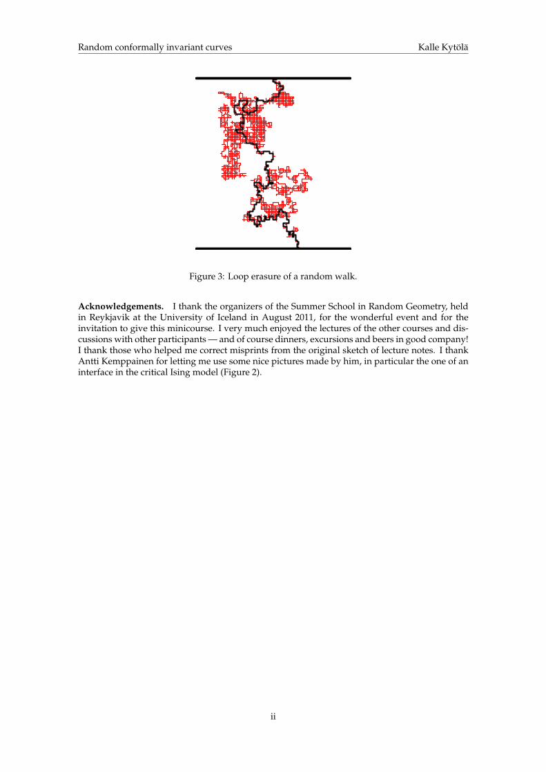
Figure 3: Loop erasure of a random walk.
Acknowledgements. I thank the organizers of the Summer School in Random Geometry, heldin Reykjavik at the University of Iceland in August 2011, for the wonderful event and for theinvitation to give this minicourse. I very much enjoyed the lectures of the other courses and dis-cussions with other participants — and of course dinners, excursions and beers in good company!I thank those who helped me correct misprints from the original sketch of lecture notes. I thankAntti Kemppainen for letting me use some nice pictures made by him, in particular the one of aninterface in the critical Ising model (Figure 2).
ii

Contents
1 Tools from complex analysis and stochastic processes 11.1 On conformal mappings . . . . . . . . . . . . . . . . . . . . . . . . . . . . . . . . . . 11.2 On stochastic calculus . . . . . . . . . . . . . . . . . . . . . . . . . . . . . . . . . . . 11
2 Introduction to Schramm-Loewner Evolutions 172.1 Schramm’s classification principles . . . . . . . . . . . . . . . . . . . . . . . . . . . . 17
3 Calculations with Schramm-Loewner evolutions 273.1 Coordinate changes of SLEs . . . . . . . . . . . . . . . . . . . . . . . . . . . . . . . . 273.2 SLE martingales constructed by domain Markov property . . . . . . . . . . . . . . 32
iii

Random conformally invariant curves Kalle Kytola
iv

Chapter 1
Tools from complex analysis andstochastic processes
To be able to work with conformally invariant random curves, we need to briefly review somebackground on conformal geometry and stochastic processes. The goal is merely to mention someof the concepts and results that will be needed later, and to provide references for them.
1.1 On conformal mappings
Below we review some facts about conformal mappings in two dimensions. Most of the statementsare proven in complex analysis textbooks such as [Ahl78], and the slightly more advanced topicsare treated for example in [Ahl73].
In differential geometry, a mapping between Riemannian manifolds is said to be conformalif the metric becomes multiplied by a positive scalar function. The angles between tangentvectors are independent of such multiplicative factor, and conformal mappings can alternativelybe defined as mappings which preserve angles. In two dimensions, for subsets of R2 = C, suchmappings are well understood — indeed from complex analysis we know that a mapping betweensubset of C preserves the magnitude of angles when it is either holomorphic (in which case alsothe orientation of angles is preserved) or anti-holomorphic (in which case the orientation of anglesis reversed). We only consider mappings that preserve the angles with orientation, so for therest of these notes a conformal mapping from one open set Λ1 ⊂ C to another Λ2 ⊂ C signifies abijective holomorphic function Λ1 → Λ2. If there exists a conformal mapping f : Λ1 → Λ2, we callthe domains Λ1 and Λ2 conformally equivalent. A conformal map f : Λ1 → Λ2 and its inversef−1 : Λ2 → Λ1 are in particular continuous, so conformal equivalence is a stronger notion thanhomeomorphism.
1.1.1 Simply connected domains and the Riemann mapping theorem
All (non-empty) connected, simply connected open subsets of C are homeomorphic to eachother, and it is a remarkable fact that with the exception of the full complex plane they are allalso conformally equivalent. A few examples of such domains, with notation that we will usethroughout these notes, are
upper half-plane H =z ∈ C : =m(z) > 0
unit disk D = z ∈ C : |z| < 1
horizontal strip S =z ∈ C : 0 < =m(z) < π
rectangle (0,Lx) × (0,Ly) =
z ∈ C : 0 <<e(z) < Lx, 0 < =m(z) < Ly
and so on. We emphasize, however, that the domains need not be as nice as the examples above —domains such as the comb ((0, 1)× (0, 1)) \∪∞n=1(i 1
n ,12 + i 1
n ]), or the interior of a fractal Jordan curve
1

Random conformally invariant curves Kalle Kytola
exemplify some wilder possibilities. The conformal equivalence of simply connected domains inknown as the Riemann mapping theorem, and here is a standard formulation of the statement.
Theorem 1 (Riemann mapping theorem) Let Λ ⊂ C be a simply connected open set such that thecomplement C \ Λ is non-empty. Then for any point z ∈ Λ there exists a unique bijective holomorphicfunction f : Λ→ D such that
f (z) = 0 and f ′(z) > 0.
Exercise 1 Show that C is not conformally equivalent to a simply connected proper subdomain Λ ( C.
To obtain a conformal map f : Λ1 → Λ2 we may use the above theorem to get conformal mapsf1 : Λ1 → D and f2 : Λ2 → D, and then set f = f−1
2 f1.The theorem also implies that a conformal map between two simply connected domains is not
unique, we were free to choose any z to be mapped to 0, and furthermore we could still rotate theimage by multiplying by any complex number of modulus one: the mapping z 7→ eiθ f (z) wouldbe conformal Λ→ D and map z 7→ 0, but the derivative at z would be on the half line eiθR+.
The non-uniqueness of the conformal map between two simply connected domains corre-sponds of course to the existence of nontrivial conformal self-maps of any of these domains: if fand f are two different conformal maps Λ → D, then f−1
f is a conformal self map of Λ whichis not the identity. It is useful to recall the explicit form of conformal self maps of some of thesimplest domains.
Lemma 1 Conformal maps f : D→ D are precisely the functions of the form
f (z) = uz − a
1 − az,
where u and a are complex parameters such that |a| < 1 and |u| = 1.
-1.0 - 0.5 0.0 0.5 1.0
-1.0
- 0.5
0.0
0.5
1.0
Figure 1.1: The radial coordinate system inD after the application of a conformal self map ofD.
Figure 1.1 illustrates the image of the radial coordinate system of D by a conformal self mapf : D→ D. The radii and circles intersect at right angles, and by conformality, so do their images.
2

Random conformally invariant curves Kalle Kytola
Lemma 2 Conformal maps f :H→ D are precisely the functions of the form
f (z) =az + bcz + d
,
where a, b, c, d ∈ R are parameters such that ad − bc > 0 (it is always possible to normalize ad − bc = 1).
- 4 - 2 0 2 40
1
2
3
4
5
Figure 1.2: A conformal self map of the upper half-plane.
Figure 1.2 illustrates the image of the Euclidean coordinate system ofH by a conformal self mapf :H→H. The horizontal and vertical lines intersect at right angles, and again by conformality,so do their images.
Let us still give two concrete examples of conformal maps between two different simplyconnected domains.
- 2 -1 0 1 2 3 4
0.0
0.5
1.0
1.5
2.0
2.5
3.0
Figure 1.3: Logarithm composed with Mobius transformation mapsH to S.
First, the map z 7→ exp(z) maps the horizontal strip S = x+ i y : x ∈ R, 0 < y < π to the upperhalf-planeH, and it is clearly holomorphic and bijective. In the other direction, if log denotes thebranch of logarithm corresponding to the choice arg ∈ [0, 2π), then z 7→ log(z) = log |z| + i arg(z)is conformalH→ S. Any conformal map fromH to S is of the form log µ, where µ : H→ H isa Mobius transformation, one such map is illustrated in Figure 1.3. The images of horizontal andvertical lines intersect forming right angles as they should.
A conformal map from the rectangle to the half-plane is given by Jacobi’s elliptic sine. Moreprecisely, denoting the elliptic modulus by k ∈ (0, 1), the rectangle is (−K,K) × (0,K′), with K =∫ π/2
0 (1− k2 sin2(θ))−1/2 dθ and K′ =∫ π/2
0 (1− (1− k)2 sin2(θ))−1/2 dθ complete elliptic integrals. Themapping z 7→ sn(z; k) then takes this rectangle conformally to H, mapping the corners −K + iK′,−K, K, K + iK′ to the points −k−1/2, −1, 1, k−1/2, respectively. Figure 1.4 illustrates this map.
3

Random conformally invariant curves Kalle Kytola
- 5 0 5
0
1
2
3
4
5
6
7
Figure 1.4: Jacobi’s elliptic function sn maps a rectangle conformally to the upper half-plane.
Mobius transformations
-1.5 -1.0 - 0.5 0.0 0.5 1.0 1.50.0
0.2
0.4
0.6
0.8
1.0
1.2
Figure 1.5: Mobius transformations map circles and straight lines to circles or straight lines. Thismap is from the unit disk to the upper half-plane.
Both of the above Lemmas concerning self maps of a simply connected domain are specialcases of the fact that any conformal map between two disks of the Riemann sphere (ordinarydisks, half-planes, exteriors of ordinary circles) is a Mobius transformation
µ(z) =az + bcz + d
, a, b, c, d ∈ C.
Conversely, the image of any circle or straight line under the a nondegenerate (ad − bc , 0)transformation of the above form is a circle or straight line. As an example, Figure 1.5 features aconformal mapD→H and shows the image of the radial coordinate system under this map.
Three real degrees of freedom in choosing a map between simply connected domains
From either of the Lemmas or the Theorem it is clear that choosing a unique conformal mapbetween two simply connected domains amounts to fixing three real parameters (the group of selfmaps of a simply connected domain is a three dimensional Lie group). We will frequently use forexample the following choices:
• If Λ1,Λ2 are simply connected domains, z1 ∈ Λ1 and z2 ∈ Λ2, and θ ∈ R then there existsa unique conformal map f : Λ1 → Λ2 such that f (z1) = z2 and f ′(z1)/eiθ > 0. (This followsdirectly from the statement of Theorem 1.)
• If Λ1,Λ2 are simply connected domains, a1, b1, c1 ∈ ∂Λ1 and a2, b2, c2 ∈ ∂Λ2 such that a j, b j, c jappear counter-clockwise along the boundaries of the respective domains Λ j, then thereexists a unique conformal map f : Λ1 → Λ2 such that f (a1) = a2, f (b1) = b2, f (c1) = c2. (Aneasy way to verify this is to construct a self map of the half plane which maps three boundarypoints to any desired images.)
4
Random conformally invariant curves Kalle Kytola
* Strictly speaking, for domains with non-Jordan boundary, boundary point is not theappropriate notion, but instead one should map the domain toD (or some other domainwith nice boundary) and consider the preimages of points of ∂D. We leave it for thecareful reader to replace the term boundary point by prime end throughtout thesenotes.
A few convenient ways of fixing the three parameters of conformal maps
We will frequently use the following choices.
f
D D \K
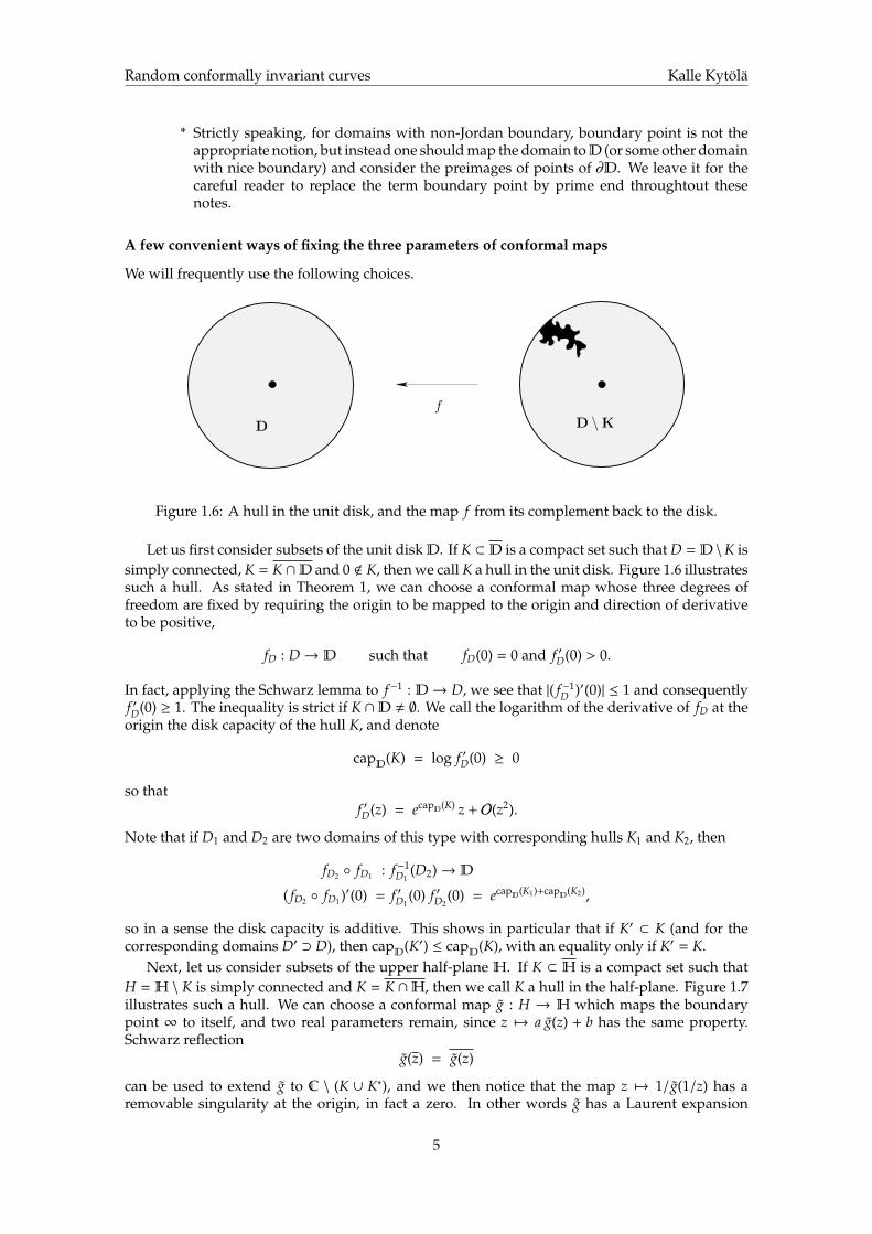
Figure 1.6: A hull in the unit disk, and the map f from its complement back to the disk.
Let us first consider subsets of the unit diskD. If K ⊂ D is a compact set such that D = D \K issimply connected, K = K ∩D and 0 < K, then we call K a hull in the unit disk. Figure 1.6 illustratessuch a hull. As stated in Theorem 1, we can choose a conformal map whose three degrees offreedom are fixed by requiring the origin to be mapped to the origin and direction of derivativeto be positive,
fD : D→ D such that fD(0) = 0 and f ′D(0) > 0.
In fact, applying the Schwarz lemma to f−1 : D→ D, we see that |( f−1D )′(0)| ≤ 1 and consequently
f ′D(0) ≥ 1. The inequality is strict if K ∩D , ∅. We call the logarithm of the derivative of fD at theorigin the disk capacity of the hull K, and denote
capD(K) = log f ′D(0) ≥ 0
so thatf ′D(z) = ecapD(K) z + O(z2).
Note that if D1 and D2 are two domains of this type with corresponding hulls K1 and K2, then
fD2 fD1 : f−1D1
(D2)→ D
( fD2 fD1 )′(0) = f ′D1(0) f ′D2
(0) = ecapD(K1)+capD(K2),
so in a sense the disk capacity is additive. This shows in particular that if K′ ⊂ K (and for thecorresponding domains D′ ⊃ D), then capD(K′) ≤ capD(K), with an equality only if K′ = K.
Next, let us consider subsets of the upper half-plane H. If K ⊂ H is a compact set such thatH = H \ K is simply connected and K = K ∩H, then we call K a hull in the half-plane. Figure 1.7illustrates such a hull. We can choose a conformal map g : H → H which maps the boundarypoint ∞ to itself, and two real parameters remain, since z 7→ a g(z) + b has the same property.Schwarz reflection
g(z) = g(z)
can be used to extend g to C \ (K ∪ K∗), and we then notice that the map z 7→ 1/g(1/z) has aremovable singularity at the origin, in fact a zero. In other words g has a Laurent expansion
5

Random conformally invariant curves Kalle Kytola
H \K H
g
Figure 1.7: A hull in the half-plane, and the map g from its complement back to the half-plane.
g(z) = cz + d + O(z−1). The free parameters a, b can be chosen so that gH(z) = a g(z) + b has theexpansion
gH(z) = z + O(z−1),
i.e. gH is as close to identity as possible in neighborhoods of infinity. We call a map with such anexpansion hydrodynamically normalized, and we call
capH(K) = limz→∞
(z (gH(z) − z)
)the half-plane capacity of the hull K, so that
gH(z) = z +capH(K)
z+ O(z−2).
Exercise 2 Show that capH(K) ≥ 0, with a strict inequality if K ∩H , ∅.
Note that if H1 and H2 are two domains of this type with corresponding hulls K1 and K2, then
gH2 gH1 : g−1H1
(H2)→H
(gH2 gH1 )(z) = = z +capH(K1) + capH(K2)
z+ O(z−2),
so in a sense the half-plane capacity is additive. In particular, if K′ ⊂ K (and for the correspondingdomains H′ ⊃ H), then capH(K′) ≤ capH(K), with an equality only if K′ = K.
Finally, let us consider subsets of the horizontal strip S. If K ⊂ S is a compact set such thatS = S \ K is simply connected, K = K ∩ S, then we call K a hull in the strip. We can choose aconformal map h : S→ S such that the boundary points ±∞ are preserved, and we still have onereal parameter to fix: the maps z 7→ h(z) + c with c ∈ R all preserve the two infinities. One canshow that the behavior of the conformal maps at ±∞ is such that the limits limz→±∞(h(z)− z) exist,so we may choose the translation c such that hS(z) = h(z) + c satisfies
hS : S→ S such that limz→+∞
(hS(z) − z) = − limz→−∞
(hS(z) − z).
We call such maps strip symmetrically normalized, and we call the quantity
capS(K) = ± limz→±∞
(hS(z) − z)
the strip capacity of the hull K, and one can show that capS(K) ≥ 0 with strict inequality if K∩S , ∅.Note that if S1 and S2 are two domains of this type with corresponding hulls K1 and K2, then
hS2 hS1 : h−1S1
(S2)→ S
limz→+∞
(hS2 (hS1 (z)) − z) = capS(K1) + capS(K2),
so in a sense the strip capacity is additive. Therefore, in particular, if K′ ⊂ K (and for thecorresponding domains S′ ⊃ S), then capS(K
′) ≤ capD(K), with an equality only if K′ = K.
6

Random conformally invariant curves Kalle Kytola
x
H
x + ih
H \ [x, x + ih]
g
- 3 - 2 -1 0 1 2 3
0
1
2
3
4
5
Figure 1.8: The complement H \ [x, x + i h] of a slit of height h located at x is mapped to thehalf-plane in such a way that at infinity the map is close to the identity.
A slit map example
Let us give one more example of explicit conformal maps. For z,w ∈ C, we denote by [z,w]the closed line segment from z to w, i.e. [z,w] = z + s(w − z) : 0 ≤ s ≤ 1. The complement inthe upper half-plane of a vertical segment (slit) starting from the real axis is a simply connecteddomainH\[x, x+ih]. Note that the boundary points of the form x+iy, 0 ≤ y < h, can be approachedeither from the left or the right of the slit, and we interpret these choices as two different boundarypoints. The reason for this becomes clear when we choose a conformal map to the half-plane. Thehydrodynamically normalized conformal map g :H \ [x, x + ih]→H is
g(z) =√
(z − x)2 + h2 + x,
where we use the branch of the square root such that√
w ∈H for all w ∈ C \ [0,∞). A map of thistype is illustrated in Figure 1.8. The two ways of approaching the boundary point x+ iy, 0 ≤ y < h,have different limits after the conformal map
limε0
(g(x − ε + i y)
)= x −
√h2 − y2
limε0
(g(x + ε + i y)
)= x +
√h2 − y2,
7

Random conformally invariant curves Kalle Kytola
as one easily sees by paying some attention to the branch of the square root.Our choice of conformal map here is such that far away the map is close to identity, g(z) =
z +O(z−1). This property manifests itself in Figure 1.8 as the fact that far away the horizontal andvertical lines of the Euclidean coordinate system are only slightly deformed. The two ways ofapproaching a boundary point on the slit can be obtained by following the (almost) horizontallines at the same height from far left and from far right: when the height of the lines is less thanthe height of the slit, these lines end at two (different) points on the interval [x − h, x + h].
1.1.2 Loewner chains
Idea of Loewner chain via infinitesimally changing conformal maps
The Riemann mapping theorem guarantees the existence of conformal maps between any twosimply connected domains, but its proof is non constructive, and typically one can only obtainexplicit formulas for the conformal maps if the domains are simple enough, as in the examples sofar.
Instead, there is a method which describes how the conformal maps vary if the domains arechanged by removing a very small piece at a well localized point. Suppose that D ⊂ D are domainsand D \ D is a small set located near a point x ∈ ∂D, and let f and f be conformal maps from Dand D, respectively, to some domain Λ. Since the two domains don’t differ by much, we try tochoose conformal maps which don’t differ by much either. We can write f = f g, with g : D→ Dis close to the identity
g(z) ≈ z + ε vx(z),
where ε measures the size of the small set D \ D in an appropriate sense, and vx : D → C is aholomorphic function specifying how we have to move each point to obtain a map D → D. It ismore appropriate to think of vx as a holomorphic vector field
vx(z) ∂z,
so that g is the flow of this vector field until time ε determined by the size of the removed pieceD \ D. Note that since ∂D and ∂D coincide except in a small neighborhood of the point x, theflow of the vector field must preserve the boundary, i.e. the vector field must be tangent to theboundary: for z ∈ ∂D \ x
vx(z) ∂z ‖ ~τz,
where ~τz is a tangent vector of ∂D at z. The holomorphic vector field must have some singularityat the boundary point x if the flow of the vector field is to remove the piece D \ D located near x. Itturns out that the singularity should be a pole, with residue such that arg(Resz=x vx(z)) = 2 arg(~τx).We will outline the argument for this in a concrete case afterwards.
A Loewner chain is a family of such continuously shrinking domains (Dt)t≥0 and their confor-mal maps (gt)t≥0, gt : Dt → D0, for which we can write the infinitesimal change of the conformalmaps as a flow of Loewner vector fields: holomorphic vector fields in D0 which are tangent to theboundary except at the point where the shrinking of the domain is located, where there is a pole.
We will make this idea more precise in concrete cases below, but let us make some commentsabout the choice of the vector field and give some examples of possible choices. First note thatit may be convenient to push forward the vector field from D0 to some nice reference domain,and do the considerations there — indeed this is necessary already to make sense of the notionsof tangent vector and residue on the boundary. Then, regarding the way we prefer to choose theconformal maps gt: if we want the maps gt to fix some point w ∈ D0, the vector fields shouldhave a zero at this point. The reader is invited to think of the algebraic restrictions on the numberand order of zeros on the boundary or in the interior of the domain. Finally, let us give three niceexamples of Loewner vector fields
• In the unit disk D, the vector fields −z z+xz−x ∂z are tangent to the boundary except at x ∈ ∂D,
and they have a simple zero at the interior point 0. These Loewner vector fields are illustratedin Figure 1.9.
8

Random conformally invariant curves Kalle Kytola
-1.0 - 0.5 0.0 0.5 1.0
-1.0
- 0.5
0.0
0.5
1.0
Figure 1.9: The Loewner vector field −z z+xz−x ∂z and its flow inD.
• In the upper half-plane H, the vector fields 2z−x ∂z are tangent to the boundary except at
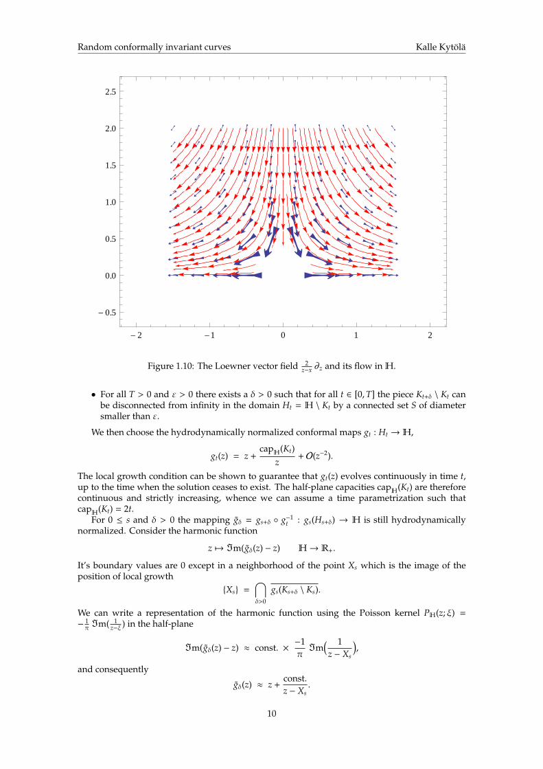
x ∈ R, and they have a zero of order two at the “boundary point”∞ (infinity is a boundarypoint if we viewH as a subset of the Riemann sphere, and to see the order of the zero, onehas to choose a local coordinate in a neighborhood of infinity). These Loewner vector fieldsare illustrated in Figure 1.10.
• In the horizontal strip S, the vector fields coth( z−x2 ) ∂z are tangent to the boundary except
at x ∈ R, and they have simple zeros at the “boundary points” ±∞. These Loewner vectorfields are illustrated in Figure 1.11.
We discuss the second case in more detail below.
Hydrodynamically normalized Loewner chain in the half-plane
Let us consider a Loewner chain in the upper half-plane H, and let us choose the conformalmaps to be as close to identity at infinity as possible. We consider a family (Ht)t≥0 of shrinkingsubdomains:
H0 =H and s < t ⇒ Hs ⊃ Ht.
We denoteKt = H \Ht,
assume that Kt are hulls in the half-plane for all t ≥ 0. We assume the hulls first of all to be strictlyincreasing, Ks ( Kt for s < t, and that K0 = ∅, and most importantly that the hulls satisfy thefollowing local growth condition
9
Random conformally invariant curves Kalle Kytola
- 2 -1 0 1 2
- 0.5
0.0
0.5
1.0
1.5
2.0
2.5
Figure 1.10: The Loewner vector field 2z−x ∂z and its flow inH.
• For all T > 0 and ε > 0 there exists a δ > 0 such that for all t ∈ [0,T] the piece Kt+δ \ Kt canbe disconnected from infinity in the domain Ht = H \ Kt by a connected set S of diametersmaller than ε.
We then choose the hydrodynamically normalized conformal maps gt : Ht →H,
gt(z) = z +capH(Kt)
z+ O(z−2).
The local growth condition can be shown to guarantee that gt(z) evolves continuously in time t,up to the time when the solution ceases to exist. The half-plane capacities capH(Kt) are thereforecontinuous and strictly increasing, whence we can assume a time parametrization such thatcapH(Kt) = 2t.
For 0 ≤ s and δ > 0 the mapping gδ = gs+δ g−1t : gs(Hs+δ) → H is still hydrodynamically
normalized. Consider the harmonic function
z 7→ =m(gδ(z) − z) H→ R+.
It’s boundary values are 0 except in a neighborhood of the point Xs which is the image of theposition of local growth
Xs =⋂δ>0
gs(Ks+δ \ Ks).
We can write a representation of the harmonic function using the Poisson kernel PH(z; ξ) =−
1π =m( 1
z−ξ ) in the half-plane
=m(gδ(z) − z) ≈ const. ×−1π=m
( 1z − Xs
),
and consequently
gδ(z) ≈ z +const.z − Xs
.
10

Random conformally invariant curves Kalle Kytola
- 6 - 4 - 2 0 2 4 6
-1
0
1
2
3
4
Figure 1.11: The Loewner vector field coth( z−x2 ) ∂z and its flow in S.
The constant has to be 2δ, by additivity of the half-plane capacity, so
1δ
(gs+δ(g−1
s (z)) − gs(g−1s (z))
)≈
2z − Xs
.
Substituting z = gs(w) we expect to get
ddt
gt(w)∣∣∣t=s =
2gs(w) − Xs
,
which indeed could be proved by doing the argument a bit more carefully.The Loewner chain (gt)t≥0 thus satisfies the Loewner differential equation
ddt
gt(z) =2
gt(z) − Xt, (1.1)
where Xt is the image under gt of the position of local growth of the hulls, a continuous functionwhich we call the driving function of the Loewner chain (gt). This is a particular case of flows ofLoewner vector fields vx(z)∂z
ddt
gt(z) = vXt (gt(z)), (1.2)
with the vector fields vx(z)∂z = 2z−x∂z which are illustrated in Figure 1.10.
Note that the slit map of Figure 1.8 exemplifies this picture: if the driving function is constantXt = x for all t ≥ 0, then the solution of gt(z) = 2/(gt(z)−x) with initial condition g0(z) = z is clearlygt(z) =
√(z − x)2 + 4t + x, the hydrodynamical conformal map fromH \ [x, x + i 2
√t] toH.
1.2 On stochastic calculus
In these notes we essentially only consider continuous stochastic processes indexed by continuoustime t.
1.2.1 Martingales and optional stopping theorem
The information we have about stochastic processes accumulates in time, and this is representedby a filtration (Ft)t≥0. The sigma algebra Ft represents information available at time t, so that in
11

Random conformally invariant curves Kalle Kytola
particular for any stochastic process (Xt)t≥0 the value Xt at time t must be measurable with respectto Ft. The information is accumulating, meaning that sigma algebras become finer, Fs ⊂ Ft fors < t. Usually we say there’s no information available at time zero, soF0 is the trivial sigma-algebra∅,Ω. Typically we also consider the information contained in a given process (Xt)t≥0, in the sensethat Ft is the smallest sigma-algebra with respect to which all Fs, + ≤ s ≤ t, are measurable.
A stochastic process (Mt)t≥0 is said to be a martingale (with respect to the filtration (Ft)t≥0) ifthe conditional expected value of the future of the process given the information at the present isthe same as the present value of the process, i.e. for all 0 ≤ s ≤ t
E[Mt
∣∣∣ Fs
]= Ms.
Roughly speaking, martingales are stochastic processes which are conserved in mean. In partic-ular, the expected value of a martingale is constant in time: with s = 0 the martingale propertyreads
E[Mt
]= M0 for any t ≥ 0.
A random time τ, whose occurrence before time t ≥ 0 can be decided with the informationavailable at time t, is called a stopping time. The optional stopping theorem states that if (Mt) is amartingale and τ is a (finite) stopping time, then
E[Mτ
]= M0.
1.2.2 Brownian motion
The standard Brownian motion onR is the process (Bt)t≥0 whose finite dimensional marginals are,for 0 < t1 < t2 < · · · < tn,
P[Bt1 ∈ A1, . . . ,Btn ∈ An
]=
∫· · ·
∫A1×···×An
exp( n∑
j=1
(x j − x j−1)2
2(t j − t j−1)
) 1∏nj=1
√2π(t j − t j−1)
dx1 · · ·dxn,
where t0 = 0 and x0 = 0. Figure 1.12 shows a realization of the Brownian motion.
0.2 0.4 0.6 0.8 1.0
-1.0
- 0.5
0.0
0.5
1.0
Figure 1.12: Values Bt of a Brownian motion are plotted on the vertical axis against t on thehorizontal axis.
A few important properties of the Brownian motion are
12

Random conformally invariant curves Kalle Kytola
• The Brownian motion is the scaling limit of simple random walks: if Sn =∑n
j=1 ξ j with ξ j
i.i.d. E[ξ j] = 0, E[ξ2j ] = 1, then the law of the process (
√δSbt/δc)t≥0 tends to the law of (Bt)t≥0
as δ 0.
• For any ε > 0, the function t 7→ Bt is (almost surely) Holder continuous with exponent 12 − ε,
but it is not Holder continuous with exponent 12 .
• The process (Bt)t≥0 is centered Gaussian and, the value at time t is mean zero variance tnormal distributed, Bt ∼ N(0,
√t).
• For any s ≥ 0, the increments Bs+t − Bs are independent of B|[0,s], and the increment process(Bs+t − Bs)t≥0 has the same law as (Bt)t≥0.
• The process (Bt)t≥0 is a martingale.
• The process (B2t − t)t≥0 is a martingale.
To check the martingale property of B2t − t, we write for 0 ≤ s < t
B2t = (Bs + Bt − Bs)2 = B2
s + 2 Bs (Bt − Bs) + (Bt − Bs)2
and recall that the increment Bt − Bs is independent of B|[0,s]. Then compute
E[B2
t − t∣∣∣ B|[0,s]
]= E
[B2
s + 2 Bs (Bt − Bs) + (Bt − Bs)2− t
∣∣∣ B|[0,s]
]= B2
s + 2 Bs E[(Bt − Bs)] + E[(Bt − Bs)2] − t
= B2s + 0 + (t − s) − t
= B2s − s.
Characterizations of the Brownian motion
The standard Brownian motion onR could also be defined as the centered Gaussian process (Bt)t≥0with covariance
E[Bt1 Bt2
]= min t1, t2 .
We will later use the fact that Brownian motion can be characterized using this property ofindependent stationary increments: if (Xt)t≥0 is a continuous real valued process with X0 = 0, suchthat for all s ≥ 0 the increment process (Xs+t−Xs)t≥0 has the same law as (Xt)t≥0 and is independentof X|[0,s], then (Xt)t≥0 has the law of (√
κBt + α t)
t≥0
for some κ ≥ 0, α ∈ R.Another characterization of the Brownian motion by Levy is the following: if (Xt)t≥0 and
(X2t − t)t≥0 are continuous martingales and X0 = 0, then X has the law of standard Brownian
motion.
1.2.3 Stochastic calculus
We will need to do calculus with differentials of Brownian motion. The reader will find a propertreatment of this stochastic calculus (or Ito’s calculus) in any of the textbooks [KS91, Oks02, RY99].Here we will give an intuitive explanation of the meaning of such calculus and most importantformulas for working with it.
We will denote by dt a differential of the time parameter t of our stochastic processes, intuitivelythis is to be interpreted as (∆t) j = t j − t j−1, where 0 = t0 < t1 < t2 < · · · is a discretization of time.Expressions involving dt are always to be integrated (or the increments (∆t) j are to be summed)over time intervals much longer than the mesh |∆| = max j(∆t) j of the discretization of time.Similarly, we will denote by dBt a differential of the Brownian motion, corresponding intuitivelyto (∆B) j = Bt j −Bt j−1 . Again, expressions involving dBt are to be integrated (or the increments (∆B) j
13

Random conformally invariant curves Kalle Kytola
are to be summed) over finite time intervals much longer than |∆| = max j(∆t) j. Note that (∆B) j isa centered Gaussian of variance (∆t) j, independent of B|[0,t j−1], and it is a good intuition that dBt isa centered Gaussian of variance dt independent of B|[0,t]. Thus the of size of dBt is of order
√dt.
For example, if σ : [0,∞)R is a given deterministic function, then multiples σ(t j−1) (∆B) j of thesmall independent centered Gaussians add up to a bigger centered Gaussian, and the expression∫ s+
s−σ(t) dBt
is Gaussian with mean 0 and variance∫ s+
s−σ(t)2 dt, independent of B|[0,s−]. Note however, that in
the above example we needed that the coefficients σ don’t depend on B.There is one important thing to pay attention to, the formula (dBt)2 = dt which may seem
counterintuitive — the squared random infinitesimal Brownian increment is deterministic in-finitesimal time increment. One naive explanation is as follows. The square of the Brownianincrement ((∆B) j)2 has the law of (∆t) j times the square of a unit normal random variable. Thusindeed the expected value is the time increment, E[((∆B) j)2] = (∆t) j. The randomness, on theother hand, has too small scale: the variance of ((∆B) j)2 is 2((∆t) j)2, so summing over a finite timeinterval with any bounded coefficients the increments squared results to a random variable whichis has variance which tends to zero as the discretization of time gets finer, |∆| = max j(∆t) j 0,hence (dBt)2 becomes deterministic and is simply given by its expected value. Expressions suchthat dBt dt and (dt)2 are zero, as the corresponding increments are of too small scale.
Ito’s formula
We consider stochastic processes (Xt)t≥0, whose infinitesimal increments have the form
dXt = αt dt + βt dBt,
where (αt) and (βt) are some processes (which are predictable with the information about theBrownian motion B up to the corresponding time instant). Such an equation for the increments iscalled stochastic differential equation, and a more appropriate meaning of it is
Xs = X0 +
∫ s
0αt dt +
∫ s
0βt dBt,
where the integrals in turn are to be understood as limits of discretizations.Note that the conditional expected value
E[ ∫ s2
s1
βt dBt
∣∣∣ B|[0,s1]
]is zero, since the integral is a sum of multiples of Brownian increments which are independentof B|[0,s1] (and the coefficients are independent of the increments due to the predictability require-ment). Therefore we expect a process (Xt) with increments dXt = αt dt + βt dBt to be a martingaleif and only if α ≡ 0 (this is only slightly too naive because of issues of existence of the expectedvalues).
We often need to know what are the increments of a process which is obtained by applyingsome function to another process. If dXt = αt dt+βt dBt and f is a twice continuously differentiablefunction, then the increments of the process ( f (Xt))t≥0 are given by Ito’s formula
d f (Xt) = f ′(Xt) βt dBt + f ′(Xt) αt dt +12
f ′′(Xt) β2t dt.
It is easy to understand this formula as a Taylor expansion with the rules (dBt)2 = dt, (dt)2 = 0and dBt dt = 0.
As a first example, we calculate
d(B2t − t) = 2 Bt dBt +
12
2 dt − dt = 2 Bt dBt.
Indeed, no dt term remains, in accordance with B2t − t being a martingale.
The Ito’s formula easily generalizes to a case where one has several independent Brownianmotions and their infinitesimal increments.
14

Random conformally invariant curves Kalle Kytola
Time changes of stochastic processes
1.2.4 Conformal invariance of two-dimensional Brownian motion
As an application of the above techniques, one can prove that the two-dimensional Brownianmotion is conformally invariant (up to a time change).
Using the conformal invariance of the two-dimensional Brownian motion and the optionalstopping theorem one for example obtains the following probabilistic interpretation of the halfplane capacity.
Exercise 3 Show that if K is a hull in the upper half-plane, (Bt) is a two-dimensional Brownian motionBt = [Bx
t ,Byt ]>, and τ = inf t ≥ 0 : Bt ∈ K ∪R, then
capH(K) = const. × limy→∞
y EB0=i y[=m(Bτ)].
This formula provides an alternative way of proving positivity of the half-plane capacity.
15

Random conformally invariant curves Kalle Kytola
16

Chapter 2
Introduction to Schramm-LoewnerEvolutions
2.1 Schramm’s classification principles
Here we give the argument, due to Oded Schramm [Sch00], ¡¡¡¡¡¡¡ .mine which identifies SLEs asthe appropriate candidates of scaling ======= which identifies SLEs as the correct candidatesof scaling ¿¿¿¿¿¿¿ .r1972 limits of interfaces in critical statistical mechanics models. When thesetup is such that all the domains we need are conformally equivalent, this Schramm’s principleclassifies all possible random curves which can be described by Loewner evolutions, which areconformally invariant, and which satisfy a natural Markovian type property. Having found theclassification, we then take that as a definition of SLE.
Conformally invariant random curves
Let us now start considering conformally invariant random curves. We thus seek to associate toeach domain Λ (with a number of marked points) a probability measure on curves in that domain,such that the push-forward of the probability measure in Λ by a conformal map f from Λ toanother domain Λ′ coincides with the probability measure associated to Λ′.
In such a consideration, we naturally restrict attention to some class of domains (with markedpoints) that are conformally equivalent. For concreteness we first discuss one of the simplestconformal types, simply connected domains Λ ⊂ C with two marked boundary points a, b ∈ ∂Λ,and look for (oriented but unparametrized) random curves from a to b in Λ. By the Riemannmapping theorem, if (Λ1; a1, b1) and (Λ2; a2, b2) are two such domains, there exists a conformalmap f : Λ1 → Λ2 such that f (a1) = a2 and f (b1) = b2, so this collection of domains indeed formsa conformal equivalence class. Note further that such conformal map is not unique, but there isa one parameter family of conformal self maps of any given domain of this type. The setup ofsimply connected domains with a random curve connecting two marked boundary points is ofterreferred to as the chordal case.
In this setup, we seek a collection (P(Λ;a,b)) of probability measures associated to domains Λwith marked boundary points a, b ∈ ∂Λ, such that for any conformal f : Λ→ f (Λ) we have
f∗ P(Λ;a,b) = P( f (Λ); f (a), f (b)).
In other words, if a random curve γ (in Λ from a to b) has the law P(Λ;a,b), then its image f γ hasthe law P( f (Λ); f (a), f (b)).
Conformal invariance alone is not a very restrictive requirement. Indeed, if we were givenany probability measure Pref on curves in one reference domain (Λref; aref, bref), subject only to thecondition that Pref is invariant under the conformal self maps of the reference domain, then wecould define the probability measures in (Λ; a, b) as f∗ Pref, where f is any conformal map fromthe reference domain to (Λ; a, b), and thus we would obtain a conformally invariant collection ofprobability measures. To find interesting conformally invariant random curves which can also
17

Random conformally invariant curves Kalle Kytola
be classified, we impose a further condition of domain Markov property, which is motivated byinterfaces in statistical mechanics.
The domain Markov property (chordal case)
aγs
Λ
b
Figure 2.1: The domain Markov property concerns the conditional law of the remaining part ofthe curve, given an initial segment γ[0, s] of it.
We still first consider the chordal setup: random curves from a ∈ ∂Λ to b ∈ ∂Λ in the closureof a simply connected domain Λ. We consider the curves as oriented but unparametrized: twoparametrized curves γ1 : [T−1 ,T
+1 ]→ C and γ2 : [T−2 ,T
+2 ]→ C are identified if γ1 = γ2 θ for some
increasing bijection θ : [T−1 ,T+1 ] → [T−2 ,T
+2 ]. An initial segment of γ : [T−,T+] → C is a restriction
of γ to a subinterval containing the beginning, i.e. γ|[T−,s] with T− ≤ s ≤ T+. The tip of an initialsegment γ|[T−,s] is the point γ(s).
The crucial assumption which adds significant content to our considerations is the following
• Domain Markov property: We assume that given any initial segment γ|[0,s] of the randomcurve γ : [0,T] → Λ in (Λ; a, b), the conditional law of the remaining part γ|[s,T] is theprobability measure associated to the domain (Λ; a, b), where Λ is component containing b ofthe complement Λ \ γ[0, s] of the initial segment and a = γ(s) is the tip of the initial segment.Put in another way,
P(Λ;a,b)
[·
∣∣∣γ|[0,s] = η]
= η P(Λ\η[0,s];η(s),b)[ · ],
wheredenotes concatenation of curves and Λ\η[0, s] is understood to stand for the relevantconnected component only.
The domain Markov property thus related the conditional law of the remaining part after aninitial segment to the law in the remaining domain. This property is motivated by interfacesin statistical mechanics models, as the reader will easily understand by considering for examplethe Ising model on a hexagonal lattice, and an interface which is a boundary between plus andminus spin clusters. In statistical mechanics, this property does not even need the model to beat a critical point. It is remarkable that when we combine the domain Markov property with theconformal invariance anticipated to emerge at the critical point, we obtain a simple classification ofthe possible random curves. This observation made in [Sch00] is known as the Schramm’s principleand will be discussed next.
The Schramm’s principle (chordal case)
For the techniques of Loewner chains to be applicable, we still have to impose the followingregularity assumption on the random curves
18
Random conformally invariant curves Kalle Kytola
• Loewner regularity: We assume that the curve γ : [0,T] → Λ starts from a, i.e. γ(0) = a, andthat the tip of any initial segment γ|[0,s] is in the component containing b of the complementΛ \ γ[0, s] of the initial segment, and that the local growth condition is satisfied.
Recall that by conformal invariance, f∗ P(Λ;a,b) = P( f (Λ); f (a), f (b)), it is enough to describe therandom curve in one reference domain, and to push-forward the definition to other domains byconformal maps. For the chordal case it is convenient to choose the reference domain (H; 0,∞),and use the chordal Loewner chain in the half-plane to describe the curve.
Assume that our collection of probability measures (P(Λ;a,b)) satisfies conformal invariance, domainMarkov property and Loewner regularity. Then let γ be a random curve in the half-plane with lawP(H;0,∞).
0
H H
gt
Xt
γt
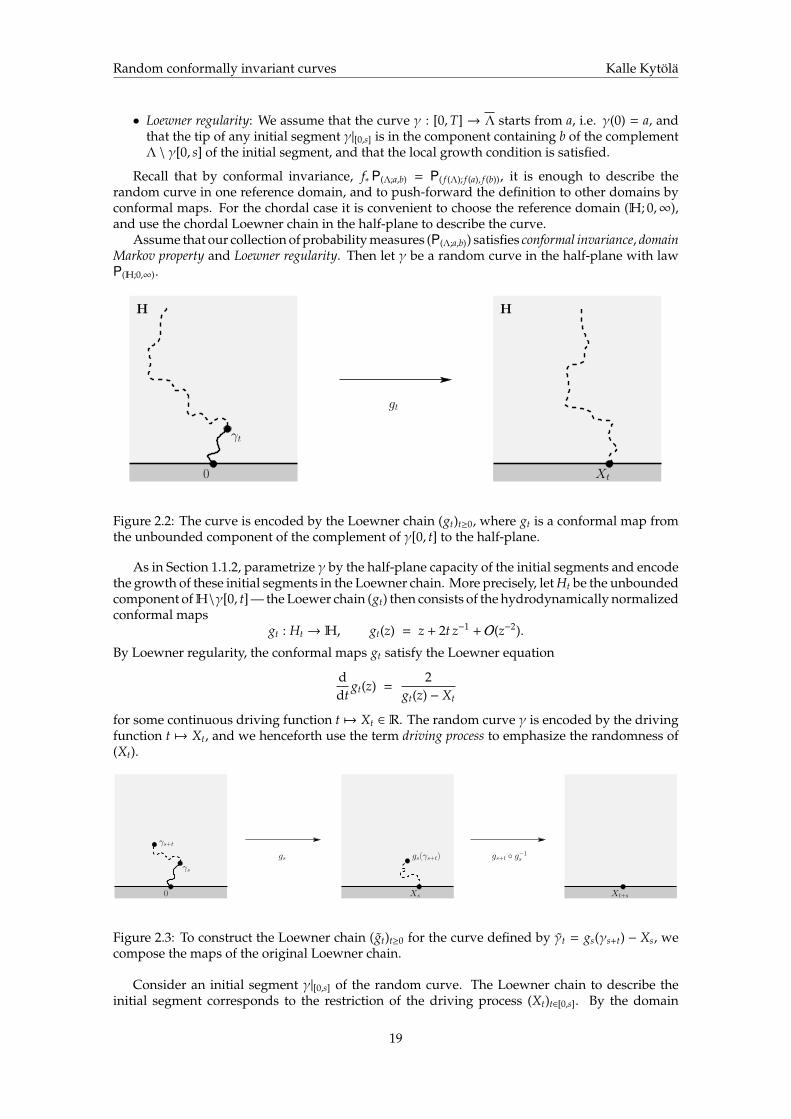
Figure 2.2: The curve is encoded by the Loewner chain (gt)t≥0, where gt is a conformal map fromthe unbounded component of the complement of γ[0, t] to the half-plane.
As in Section 1.1.2, parametrize γ by the half-plane capacity of the initial segments and encodethe growth of these initial segments in the Loewner chain. More precisely, let Ht be the unboundedcomponent ofH\γ[0, t] — the Loewer chain (gt) then consists of the hydrodynamically normalizedconformal maps
gt : Ht →H, gt(z) = z + 2t z−1 + O(z−2).
By Loewner regularity, the conformal maps gt satisfy the Loewner equation
ddt
gt(z) =2
gt(z) − Xt
for some continuous driving function t 7→ Xt ∈ R. The random curve γ is encoded by the drivingfunction t 7→ Xt, and we henceforth use the term driving process to emphasize the randomness of(Xt).
0
γs
gs
Xs Xt+s
gs+t g−1sgs(γs+t)
γs+t
Figure 2.3: To construct the Loewner chain (gt)t≥0 for the curve defined by γt = gs(γs+t) − Xs, wecompose the maps of the original Loewner chain.
Consider an initial segment γ|[0,s] of the random curve. The Loewner chain to describe theinitial segment corresponds to the restriction of the driving process (Xt)t∈[0,s]. By the domain
19

Random conformally invariant curves Kalle Kytola
Markov property, the conditional law of the remaining part γ|[s,T] given the initial segment isP(Hs;γ(s),∞). Now note that the map
z 7→ gs(z) − Xs
is conformal from Hs to H, and such that γ(s) 7→ 0 (definition of driving function) and ∞ 7→∞ (hydrodynamical normalization). Therefore, conditionally on the initial segment, conformalinvariance states that the law of the image of γ|[s,T] by the map gs − Xs has the law P(H;0,∞). Theimage curve γ is defined by
γ(t) = gs(γ(s + t)) − Xs, t ≥ 0.
Let (gt) denote the collection of hydrodynamically normalized conformal maps gt : Ht → H,where Ht is the unbounded component ofH \ γ[0, t]. In fact,
z 7→ gs+t
(g−1
s (z + Xs))− Xs
is a conformal map Ht →H, and it is a matter of simple calculation to verify the normalization
gs+t
(g−1
s (z + Xs)︸ ︷︷ ︸≈ z+Xs−
2sz+Xs
+···
)− Xs =
(z + Xs −
2sz + Xs
+ · · ·)
+2(s + t)
z + Xs −2s
z+Xs+ · · ·
+ · · · − Xs
=(z + Xs −
2sz
)+
2(s + t)z
− Xs + O(z−2)
= z +2tz
+ O(z−2).
We see that not only is the above map hydrodynamically normalized, but also the curve γ is stillparametrized by capacity. In conclusion the Loewner chain for γ is given by
gt(z) = gs+t
(g−1
s (z + Xs))− Xs.
This Loewner chain must satisfy a Loewner’s equation of the form
ddt
gt(z) =2
gt(z) − Xt,
and indeed from the expression above we calculate
ddt
gt(z) =ddt
(gs+t
(g−1
s (z + Xs))− Xs
)=
2
gs+t
(g−1
s (z + Xs))− Xs+t
=2
gt(z) + Xs − Xs+t.
We get that the driving process of (gt) is given by the increment of the driving process of (gt)
Xt = Xs+t − Xs.
Moreover, since γ has the same law P(H;0,∞) as γ, the driving process (Xt) must have the same law as(Xt). Also recall that the considerations so far were done conditionally on the initial segment γ|[0,s]or equivalently conditionally on its driving function (Xt)t∈[0,s], so by we see that (Xt) is independentof (Xt)t∈[0,s]. The continuous process (Xt) therefore has independent and identically distributedincrements, so its law is necessarily that of a multiple of Brownian motion plus linear drift(
Xt
)t≥0
in law≡
(√κBt + α t
)t≥0, κ ≥ 0, α ∈ R.
However, we now check that only α = 0 is consistent with the requirement that P(H;0,∞) is invariantunder the one parameter family of conformal self maps of (H; 0,∞). These self maps are thescalings of the half-plane, z 7→ λz for λ > 0. To map complements of initial segments λγ[0, t] ofthe scaled curve λγ hydrodynamically to the half-plane, one uses the map
z 7→ λ gt(z/λ).
20

Random conformally invariant curves Kalle Kytola
The Laurent expansion
λ gt(z/λ) = λ(z/λ +
2tz/λ
+ · · ·)
= z +2λ2t
z+ · · ·
reveals that the correct capacity parametrization of λγ is
γ(λ)(t) = λγ(λ−2t).
The capacity parametrized Loewner chain for λγ is (g(λ)t ) with
g(λ)t (z) = λ gλ−2t(z/λ).
The Loewner equation satisfied by this Loewner chain is obtained by calculating the time deriva-tive
ddt
g(λ)t (z) = λλ−2 2
gλ−2t(z/λ) − Xλ−2t=
2λ gλ−2t(z/λ) − λXλ−2t
=2
g(λ)t (z) − λXλ−2t
,
from which we see that the driving process (X(λ)t ) of (g(λ)
t ) is
X(λ)t = λXλ−2t.
If Xt ≡√κBt + αt, then
X(λ)t ≡ λ
(√κBλ−2t + αλ−2t
)≡ λ√κ√
λ−2 Bt + λαλ−2t ≡√κBt + αλ−1t.
The scaled curve λγ would have a different law if α , 0, so the conformal invariance under selfmaps of (H; 0,∞) requires α = 0 and finally
Xt ≡√κBt.
We have obtained a strong classification: if a random conformally invariant chordal curvesatisfies domain Markov property (and Loewner regularity), then the curve is the push forwardby conformal maps from the half-plane (H; 0,∞) of a curve whose Loewner driving process is amultiple of Brownian motion. The requirements we imposed motivated by interfaces in criticalmodels of statistical mechanics characterized the law of a curve up to one parameter κ.
2.1.1 The chordal SLEκThe conclusion obtained by Schramm’s principle is that there can be no other conformally invariantchordal random curves with domain Markov property except the ones whose half-plane Loewnerchain has driving process (
√κBt)t≥0 for some κ ≥ 0. We thus call the Loewner chain determined
by
g0(z) = z,ddt
gt(z) =2
gt(z) − Xt, Xt =
√κBt
the chordal Schramm-Loewner evolution with parameter κ in (H; 0,∞), or briefly chordal SLEκ in(H; 0,∞).
A priori the chordal SLEκ is a collection of conformal maps (gt)t≥0, where gt : H \ Kt → H is ahydrodynamically normalized map from complements of random hulls Kt ⊂H, and the hulls aregrowing: Kt ⊂ Ks for t < s. It is however natural to ask whether there is a curve γ : [0,∞)→H suchthat Kt = γ[0, t], or if at least Kt is generated by a curve in the sense thatH \ Kt is the unboundedcomponent ofH \ γ[0, t]. The following result answers the latter question in the affirmative.
Theorem 2 (Rohde and Schramm, [RS05]) For the chordal SLEκ in (H; 0,∞), the limits
γ(t) = limε0
g−1t (Xt + iε)
exist and depend continuously on t ≥ 0. We call the curve γ the chordal SLEκ trace in (H; 0,∞). Thehulls (Kt) are generated by the trace.
21

Random conformally invariant curves Kalle Kytola
The proof is somewhat lengthy although not particularly difficult, and in fact the case κ = 8 needsto be considered separately — it was completed in [LSW04]. The interested reader will find acareful proof in the generic case κ , 8 in [Law10].
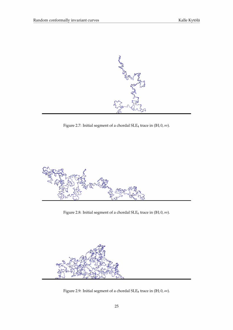
Admitting the above result on the chordal SLE trace, we from here on view the chordal SLEκas a random curve rather than a Loewner chain. This is certainly closer to the original motivation,and it is worth emphasizing that the curve is the fundamental object, whereas the Loewner chain ismerely an artefact resulting from our description of the curve. Figures 2.4 — 2.9 portray simulatedchordal SLEκ traces for a few different values of κ.
Figure 2.4: Initial segment of a chordal SLE2 trace in (H; 0,∞).
We immediately remark the invariance under conformal self-maps of a domain (Λ; a, b). In thefollowing form it directly follows from the scaling calculation we did in the course of establishingthe Schramm’s principle in the chordal case.
Proposition 1 The law of chordal SLEκ in (H; 0,∞) is invariant under the scalings z 7→ λz, λ > 0.
It is also natural to ask for other properties of SLEs. The following result on the qualitativeproperties divides the parameter regions of κ to three phases.
Theorem 3 (Rohde and Schramm, [RS05]) The (trace of the) chordal SLEκ in (H; 0,∞) is transient,
limt∞
γ(t) = ∞,
and it has the following properties according to the parameter κ ≥ 0
0 ≤ κ ≤ 4: The trace γ : [0,∞)→H is a simple curve, and γ(t) ∈H for all t > 0.
4 < κ < 8: For any z ∈ H almost surely there exists a t > 0 such that z ∈ Kt but z < γ[0, t], i.e.the trace surrounds (or “swallows”) the point z without passing through it. Also γ[0,∞) ∩ R isunbounded.
κ ≥ 8: The trace is a space filling curve, γ[0,∞) =H, i.e. the trace visits every point of the domain.
22

Random conformally invariant curves Kalle Kytola
Figure 2.5: Initial segment of a chordal SLE8/3 trace in (H; 0,∞).
We will prove some of the statements in the next chapter, the others could be proven by quitesimilar techniques.
The simulated pictures give some hints about the three phases, although due to the necessarydiscretization of the curves for the simulation, the pictures have no genuinely different phases. Itis also somewhat challenging to reduce numerical errors in simulating SLEs, so from the picturesit might not be clear that phase transitions occur at the precise values of the parameter κ.
One of the most notable quantitative properties of chordal SLEκ is the fractal dimension.Looking at the simulated pictures, one may already guess that the fractal dimension of the curveincreases with the parameter κ.
Theorem 4 (Beffara, [Bef08]) For 0 ≤ κ ≤ 8, the Hausdorff dimension of γ, the trace of the chordalSLEκ, is 1 + κ
8 . For κ > 4, the Hausdorff dimension of ∂Kt, the boundary of the SLE hull, is 1 + 2κ .
It is not very difficult to obtain the sharp upper bound for the Hausdorff dimension, and in the nextchapter we present an argument which leads to the correct value of the dimension. A reasonablyaccessible and careful proof of the entire result can be found in [Law10].
2.1.2 Other SLEs
It turns out that Schramm’s principle works rather well in a few of the simplest situtations besidesjust the chordal case, notably the following:
• random curves in simply connected domains with three marked boundary points
• random curves in simply connected domains with a marked boundary point and a markedinterior point
In each of the two cases, Riemann mapping theorem guarantees that any two domains are con-formally equivalent, and in these cases there are no conformal self maps of a domain — all threedegrees of freedom are needed to fix the marked points. We may thus expect that the conformalinvariance requirement is somewhat less restrictive, and indeed we will find that the classificationleaves room for an additional parameter.
23

Random conformally invariant curves Kalle Kytola
Figure 2.6: Initial segment of a chordal SLE3 trace in (H; 0,∞).
Exercise 4 Find a Schramm’s principle for Loewner regular conformally invariant curves with domainMarkov property in the following situation: the domain Λ ( C is simply connected, the curve start fromboundary point a ∈ ∂Λ, and the law P(Λ;a,b,c) depends also on two other marked boundary points b, c ∈ ∂Λ.Hint: It is convenient to work in (S; 0,+∞,−∞), and use a Loewner chain corresponding to Loewner vectorfields coth( z−x
2 ) ∂z.
One could also consider other configurations, such as four or more marked boundary pointsin simply connected domains, or more marked interior points, or multiply connected domains.In each of these cases, however, there are conformal moduli, i.e. two generic such domainsare no longer conformally equivalent. The requirement of conformal invariance then has weakerconsequences, and an attempt of classification as above becomes less satisfactory — in applicationsto statistical mechanics models one needs more input from the model itself for identifying theappropriate random curves.
24
Random conformally invariant curves Kalle Kytola
Figure 2.7: Initial segment of a chordal SLE4 trace in (H; 0,∞).
Figure 2.8: Initial segment of a chordal SLE6 trace in (H; 0,∞).
Figure 2.9: Initial segment of a chordal SLE8 trace in (H; 0,∞).
25

Random conformally invariant curves Kalle Kytola
γ[0, t]
H HH
γ[0, t]
Kt
0 ≤ κ ≤ 4 4 < κ < 8 8 ≤ κ
Figure 2.10: According to the value of the parameter κ, SLE is in one of the three qualitativelydifferent phases: the trace γ is either a simple curve, a self-touching curve, or a space filling curve.
26

Chapter 3
Calculations with Schramm-Loewnerevolutions
In this minicourse we present two key techniques for calculating things with SLEs:
• Coordinate changes of SLEs
• Matringales from domain Markov property.
We give a few examples of each of the two techniques, chosen so that the calculations remainsimple enough but at the same time illustrate and emphasize some important properties of SLEcurves.
It is very common that the two techniques are combined together to derive an interestingproperty of SLEs, like in the case of the restriction property of chordal SLE8/3 which can be found inalmost any introduction to SLEs. Often the calculations also allow for natural interpretations usingGirsanov’s theorem — a change of drift of the driving process resulting either from coordinatechanges or conditioning on an event can be seen as a weighting of the SLE probability measureby a martingale. We will only comment on these interpretations briefly.
3.1 Coordinate changes of SLEs
In this section we consider descriptions of the same random curve by different Loewner chains. Weemphasize that the random curve is the fundamental object and its parametrization and Loewnerchain description are somewhat arbitrary choices, although certain choices are without a doubtmore convenient than others.
The article [?] does several coordinate changes systematically. The same idea and almostidentical calculations are fundamental for many different SLE problems, so variations on thistheme have appeared in the literature ever since SLEs were introduced.
The chordal SLE in half-plane with another endpoint
We have defined the chordal SLEκ in H from 0 to ∞ as the curve which generates the Loewnerchain with driving process (
√κBt)t≥0. In any other domain (Λ; a, b), the chordal SLEκ is the image
of this curve by a conformal map from (H; 0,∞) to (Λ; a, b).Let us consider the case where the domain is still the half-planeH, the starting point still the
origin, but the end point is some point b ∈ R \ 0 at finite distance. The chordal SLEκ in (H; 0, b)is clearly a Loewner regular curve (up to the first time it disconnects b from infinity), so we cangive a description of it by a chordal Loewner chain.
So, let γ : [0,∞)→H be the chordal SLEκ trace in (H; 0,∞) parametrized by capacity as above,and let γ(t) = µ(γ(t)), where µ is a conformal map from (H; 0,∞) to (H; 0, b). Such conformal mapsare Mobius transformations, and there is a one parameter family of them:
µ(z) =b z
z − s
27

Random conformally invariant curves Kalle Kytola
where the parameter s ∈ R\0 is the point whose image under µ is infinity. We will use a Loewnerchain that fixes infinity to describe the image curve γ = µ γ, so in a sense we are observing theoriginal SLE curve in (H; 0,∞) from the point s.
Let (gt)t≥0 be the Loewner chain defining the chordal SLEκ in (H; 0,∞),
g0(z) = z,ddt
gt(z) =2
gt(z) − Xt, Xt =
√κBt.
We want to find the Loewner chain that describes γ = µ γ, the chordal SLEκ in (H; 0, b). To thisend, let gt be the hydrodynamically normalized conformal map from the unbounded componentHt ofH \ γ[0, t] toH. Note that γ is not yet parametrized by capacity, but it is not difficult to seethat it would only take a differentiable change of parametrization to achieve that. Let us denoteby st the half-plane capacity of the hull generated by γ[0, t], so that gt(z) = z+2st z−1 +O(z−2). Thenby Loewner regularity of the image curve γ, until the time that γ disconnects b from∞we have
g0(z) = z,ddt
gt(z) =2 st
gt(z) − ξt
for some driving process (ξt)t≥0, and with st = ddt st the speed of capacity growth of γ.
We already have at our disposal the conformal map gt µ−1 : Ht →H. The hydrodynamicallynormalized conformal map gt : Ht → H is obtained by post-composing with an appropriate selfmap µt of the half-plane,
gt = µt gt µ−1.
One could give an explicit expression for the time dependent Mobius transformation µt, but itturns out to be not necessary. We note that the driving process (ξt) is the image under the Loewnerchain (gt) of the tip of γ, or alternatively
ξt = gt
(γ(t)
)=
(µt gt µ
−1)(µ(γ(t))
)= µt(Xt).
Also sinceµt = gt µ g−1
t ,
we can calculate the time derivative of µt(z). We just recall the Loewner equation for gt, andobserve that the time derivative of g−1
t is easily read from
0 =ddt
(z) =ddt
(gt(g−1
t (z)))
=2
gt(g−1t (z)) − Xt
+ g′t(g−1t (z))
( ddt
g−1t (z)
)),
with the resultddt
g−1t (z) =
−2 (g−1t )′(z)
z − Xt.
Now we calculate the time derivative of µt as follows
ddtµt(z) =
ddt
(gt(µ(g−1
t (z))))
=2 st
gt(µ(g−1t (z))) − ξt
+ (gt µ)′(g−1t (z))
−2 (g−1t )′(z)
z − Xt
=2 st
µt(z) − ξt−
2µ′t(z)z − Xt
.
The Mobius transformation µt :H→H, and its time derivative as well, is regular at the point Xton the boundary (the only pole of µt is at the point gt(s), so that gt = µt gt µ−1 fixes infinity).Therefore, the poles at z→ Xt of the two terms in d
dtµt(z) must cancel. We do a Laurent expansionfor the first term, keeping in mind that µt(Xt) = ξt,
2 st
µt(z) − ξt=
2 st(ξt + µ′t(Xt) (z − Xt) + 1
2µ′′
t (Xt) (z − Xt)2 + · · ·)− ξt
=2 st
µ′t(Xt) (z − Xt)−
st µ′′t (Xt)µ′t(Xt)2 + O(z − Xt).
28

Random conformally invariant curves Kalle Kytola
The second term is even easier
−2µ′t(z)z − Xt
=−2µ′t(Xt)
z − Xt− 2µ′′t (Xt) + O(z − Xt).
For the poles to cancel, we must have
st = µ′t(Xt)2.
This is of course intuitive. On the one hand, st is the speed of capacity growth of the curve γ attime t. On the other hand, a small piece of the curve γ[t, t + ∆t] becomes, after mapping to thehalf-plane by gt, the image of gt(γ[t, t + ∆t]) under µt. But gt(γ[t, t + ∆t]) is a small piece of curve inH of capacity ∆t, and it is located near Xt. So µt essentially scales this piece by the factor µ′t(Xt) andthe image has capacity approximately µ′t(Xt)2 ∆t, which is the asserted capacity growth st+∆t − st.
We made the expansions at z → Xt of the two terms in ddtµt(z) up to constant terms, so we
immediately read the time derivative of µt at the point Xt,( ddtµt
)(Xt) = −3µ′′t (Xt).
This facilitates the determination of the driving process (ξt) of the Loewner chain (gt) sinceξt = µt(Xt), as we observed earlier. Now, recalling that dXt =
√κdBt, the Ito derivative of ξt is
dξt = d(µt(Xt)
)= µ′t(Xt)
√κ dBt +
κ2µ′′t (Xt) dt +
( ddtµt
)(Xt) dt
= µ′t(Xt)√κ dBt +
κ − 62
µ′′t (Xt) dt.
We may further remark that any Mobius transformation ν has the property
ν′(z)2
ν′′(z)=
12
(ν(z) − ν(∞)
).
Applied to µt at Xt, noting µt(∞) = gt(b), this gives
µ′′t (Xt)µ′t(Xt)2 =
2ξt − gt(b)
,
which allows us to simplify the Ito derivative of ξt to
dξt =√κ st dBt +
κ − 6ξt − gt(b)
st dt.
In order to have a standard Loewner chain description of γ, the chordal SLEκ in (H; 0, b), weshould use s = st as the time parameter. Denote by s 7→ ts the inverse function of t 7→ st. Then theLoewner equation takes the usual form
dds
gts (z) =2
gts (z) − ξts
and the change of time parametrization of the driving process leads to
dξts =√κ dBs +
κ − 6ξt − gt(b)
ds,
where (Bs)s≥0 is a standard Brownian motion with respect to the time parameter s. This displaysthat the change of the chordal SLE endpoint to b excerts a drift on the driving process, whosestrength is inversely proportional to the conformal distance of the tip and the endpoint. The signand strength of the drift depend on κ, and at κ = 6 the additional drift vanishes.1
1This particular phenomenon at κ = 6 gets a natural interpretation from a percolation result of Smirnov. The chordalSLE6 is the scaling limit of exploration path of critical percolation — and the exploration path doesn’t feel where itsdeclared endpoint is.
29

Random conformally invariant curves Kalle Kytola
The Loewner chain (gts )s≥0 is of the form that is usually taken as definition of the SLE variantSLEκ(ρ) in the domain (H; 0, b,∞), with the particular value ρ = κ− 6 here. Below we will discussthe Schramm’s principle applied to simply connected domains with three marked boundarypoints, and conclude that the most general (Loewner regular) conformally invariant randomcurves with domain Markov property are SLEκ(ρ), for κ ≥ 0 and ρ ∈ R. In view of this fact, theresult of the coordinate change had to be of this form.
The process SLEκ(κ − 6) is also instrumental for the construction of so called conformal loopensembles via an exploration tree, but for this purpose the process has to be continued in aslightly nontrivial fashion beyond the first time that the curve disconnects the target point b fromthe observation point ∞. This is beyond the scope of the present minicourse, but the interestedreader may consult the article [She09] for further information.
SLEs with three marked boundary points
In an earlier exercise, the following version of Schramm’s principle was considered. To eachsimply connected domain Λ ( C and three boundary points a, b, c ∈ ∂Λ one associates a probabilitymeasure P(Λ;a,b,c) on Loewner regular curves starting from a and ending on the arc bc, and suchthat conformally invariance holds in the sense that f∗P(Λ;a,b,c) = P( f (Λ); f (a), f (b), f (c)) for f a conformalmap. The classification result is that such curve in (S; 0,+∞,−∞) must be described by a Loewnerchain
h0(z) = z,ddt
ht(z) = coth(ht(z) − Vt
2
), Vt =
√κBt + α t,
for some κ ≥ 0 and α ∈ R. In other domains the curve can be defined by conformal transport,as the image of the curve in (S; 0,+∞,−∞) under a conformal map f : S → Λ such that f (0) = a,f (+∞) = a, f (−∞) = c.
For easier comparison with the chordal SLE, let us take the curve in the upper half-plane sothat it starts from the origin and one of the marked points is at infinity. To obtain the curve in(H; 0,∞, c), where c < 0, we use the conformal map f from S toH such that f (0) = 0, f (+∞) = ∞and f (−∞) = c.
A formula for that map isf (z) = |c|(ez
− 1).
Let η : [0,∞) → S be the curve in (S; 0,+∞,−∞) and consider the image γ(t) = f (η(t)). Thecomponent of S \ η[0, t] which contains both ±∞ is denoted by St and the Loewner chain (ht)t≥0consists of conformal maps ht : St → S normalized so that ht(z) − z → ±t as z → ±∞. The curveγ is Loewner regular, too, and Ht = f (St) is the component of H \ γ[0, t] which contains infinity(and c). Again, the curve γ as we define it is not parametrized by half-plane capacity, but ittakes a C1 reparametrization to achieve this. Denote again by st half the half-plane capacity ofthe hull generated by γ[0, t], so that if gt : Ht → H is the hydrodynamical conformal map, thengt(z) = z + 2stz−1 + O(z−2). The maps (gt) satisfy the Loewner flow equation
ddt
gt(z) =2 st
gt(z) − Xt,
where st = ddt st is half the speed of capacity growth and Xt is the image of the position of local
growthXt = gt(γ(t)) = gt( f (η(t))).
We have at our disposal one conformal map from Ht toH, namely the composition f ht f−1,but it is not hydrodynamically normalized. The hydrodynamically normalized maps can beobtained by post-composing with the appropriately chosen conformal self map ofH,
gt = µt f ht f−1,
where µt : H → H is a Mobius transformation. In this situation µt preserves infinity, so wecan write µt(z) = at z + bt, and it turns out not to be necessary to write down at and bt explicitly
30

Random conformally invariant curves Kalle Kytola
(although it is not difficult to do so, and the reader should perhaps nevertheless do that as anexercise). For brevity, let us also denote by
ϕt = µt f = gt f h−1t
the conformal map S→Hwhich is important for us at time t. This map in particular gives us thedriving process of γ,
Xt = ϕt(Vt).
We will next calculate the time derivative of the map ϕt. For this purpose we need the timederivative of h−1
t , and we leave it as an easy exercise for the reader to check that
ddt
h−1t (z) = −(h−1
t )′(z) coth(z − Vt
2
).
Using this and the Loewner flow equation for gt, we write the time derivative we are interestedin as
ddtϕt(z) =
ddt
(gt( f (h−1
t (z))))
=( ddt
gt
)( f (h−1
t (z))) + (gt f )′(h−1t (z)))
( ddt
h−1t
)(z)
=2 st
gt( f (h−1t (z))) − Xt
− (gt f )′(h−1t (z))) (h−1
t )′(z) coth(z − Vt
2
)=
2 st
ϕt(z) − Xt− ϕ′t(z) coth
(z − Vt
2
).
Taylor expansion of the two terms at z = Vt like before gives
ddtϕt(z) =
1z − Vt
( 2 st
ϕ′t(Vt)− 2ϕ′t(Vt)
)−
st
ϕ′t(Vt)2 − 2 ϕ′′t (Vt) + O(z − Vt).
The maps ϕt as well as their derivatives are regular at the boundary point Vt, so we require thepole to cancel, and obtain the equation
st = ϕ′t(Vt)2,
which again is the intuitive property resulting from the change of capacity under the approximatescaling that ϕt does in neighborhoods of Vt. So we have an expression for the (explicit) timederivative of ϕt at the point Vt ( d
dtϕt)(z) = −3ϕ′′t (Vt) + O(z − Vt).
We are in a position to compute the increment of Xt = ϕt(Vt) by Ito’s formula, recalling alsodVt =
√κdBt + αdt. The result is
dXt = d(ϕt(Vt)
)=
( ddtϕt)(Vt) dt + (
√κ dBt + α dt) ϕ′t(Vt) +
κ2
dt ϕ′′t (Vt)
=√κ st dBt +
(κ − 62
ϕ′′t (Vt)ϕ′t(Vt)2 + α
1ϕ′t(Vt)
)st dt.
We leave it for the reader to verify using the expressions we have found so far, that
ϕ′′t (Vt)ϕ′t(Vt)2 =
1Xt − gt(c)
=1
ϕ′t(Vt).
Then we may perform a time change to the the half-plane capacity time parameter s, under whichwe have the ordinary
dds
gts (z) =2
gts (z) − Xts
.
31
Random conformally invariant curves Kalle Kytola
The driving process becomes
d(Xts ) =√κ dBs +
(κ − 62
+ α) 1
Xts − gts (c)ds.
The driving process of the image curve is the one that defines SLEκ(ρ) in (H; 0,∞, c), withρ = κ−6
2 + α. We have thus shown by a Schramm’s principle (the exercise with three markedboundary points) and a coordinate change that the most general Loewner regular conformallyinvariant random curve which satisfies the domain Markov property and depends on threeboundary points of a simply connected domain, is SLEκ(ρ), for κ ≥ 0 and ρ ∈ R.
As a notable example, the curve η would have been a chordal SLEκ in (S; 0,+∞) if α = 6−κ2 .
Reflecting the sign of the drift α, the chordal SLEκ in (S; 0,−∞) would have α = κ−62 , and coming
back to the half-plane picture, the chordal SLEκ in (H; 0, c) corresponds to ρ = κ− 6 as we alreadyfound before.
3.2 SLE martingales constructed by domain Markov property
One of the most important ways of calculating things with SLEs consists in finding a martingalewhose end value is the quantity of interest. The domain Markov property provides a natural wayof constructing martingales that compute relevant quantities. We will illustrate this techniquein two example cases. The first example is a computation of the probability that the chordalSLEκ touches a given boundary arc. This case explains first of all why κ = 4 is the point ofphase transition from simple curves to self-touching curves, and it also gives a certain crossingprobability that is interesting in the statistical mechanics models. The second example concernsthe dimension of the SLE trace. Here we in fact only state a property which gives an upper boundfor the Hausdorff dimension, and furthermore we only give a heuristic derivation, which couldbe made rigorous by slightly altering the definitions and putting in a little bit of extra work. Therigorous derivation can be found in the literature, but the heuristic derivation is shorter and atleast as enlightening as the proper one.
Boundary visits of chordal SLE
Let γ(Λ;a,b) denote the chordal SLEκ trace in the domain Λ from a ∈ ∂Λ to b ∈ ∂Λ. Our goal is tofind an expression for
P[γ(Λ;a,b)
∩ A , ∅],
where A ⊂ ∂Λ \ a, b is an arc of the boundary of the domain. By conformal invariance, it issufficient to find an answer in the reference domain (H; 0,∞).
The phase transition at κ = 4
The first thing we show is that the chordal SLEκ only touches the boundary when κ > 4. If thechordal SLEκ trace γ in (H; 0,∞) touches the boundary at a point x ∈ (0,∞), then all the pointsx′ ∈ (0, x) are disconnected from infinity by the curve, and they belong to the SLE hull after thetime s such that γ(s) = x. Furthermore, by the scale invariance stated in Proposition 1, either allx′ > 0 have a positive probability to become part of the hull, or no x′ > 0 ever becomes a part ofthe hull. The question of whether the trace can touch the boundary at any other point but thestarting point a = 0 and the end point b = ∞, is equivalent to whether the boundary points canbecome a part of the hull.
Recall that the hull Ks is defined as the set of points z ∈H such that the Loewner equation
ddt
Zt =2
Zt − Xt
with initial conditionZ0 = z ∈H
32

Random conformally invariant curves Kalle Kytola
has no solution up to time s, i.e. that the denominator Dt = Zt − Xt becomes zero before thetimes s (or at least its values accumulate at 0). The denominator is governed by the Ito stochasticdifferential equation
dDt =2
Dtdt −
√κ dBt.
This is in fact just a time change of the familiar Bessel process: if t(u) = u/κ, then with respect tothe time parameter u we have
dDt(u) =2/κDt(u)
du + dBu,
where (Bu)u≥0 is a standard Brownian motion: Bu = −√κBu/κ. Recall that the Bessel process (βt)
of dimension d is defined by the Ito stochastic differential equation
dβt =(d − 1)/2
βtdt + dBt,
and for integer d it corresponds to the absolute value of the d-dimensional Brownian motion. TheBessel process hits the origin in finite time (when started away from the origin) if and only if d < 2.Comparing the equations we equate d = 1 + 4/κ, and correspondingly the denominator processDt hits zero if and only if κ > 4.
We have shown that the chordal SLEκ trace touches the boundary if and only if κ > 4. Thereader may judge to which extent the pictures 2.4 – 2.9 plausibly illustrate this phenomenon. Let usfurthermore remark that SLE’s touching the boundary is equivalent to self touching of the curve.Indeed, suppose that the chordal SLEκ trace γ in (H; 0,∞) has a double point γ(t1) = γ(t2) for0 ≤ t1 < t2. Pick s ∈ (t1, t2), and consider conditioning on γ[0, s]. By the domain Markov property,the conditional law of γ[s,∞) is the law of chordal SLEκ in (Ht;γ(s);∞). But if γ(t2) = γ(t1), thenthe point γ(t2) on the curve γ[s,∞) is not in the interior of the domain Ht, which means that thechordal SLEκ touches the boundary of its domain (by conformal invariance it doesn’t matter inwhich domain this happens). Thus, admitting the existence of the chordal SLE trace, we haveshown the first phase transition stated in Theorem ??: for κ ≤ 4 the trace is a simple curve whichdoesn’t touch the boundary of the domain, and for κ > 4 the trace has double points and touchesthe boundary.
The martingale and the probability to touch a boundary interval
Let us then compute the probability for the chordal SLEκ, κ > 4, to touch a boundary arc. Theequivalent question in the half-plane is to compute
P(z−, z+) = P[γ(H;0,∞)
∩ [z−, z+] , ∅],
where 0 < z− < z+, say (intervals on the negative real axis are handled similarly). The techniqueto do so relies on finding a martingale whose end value is the indicator of the event that theboundary interval is touched.
The conditional expected values of any random variable, conditioned on the initial segmentsγ(H;0,∞)[0, t], t ≥ 0, constitute a martingale by construction. In particular, the conditional probabil-ities
Mt = P[γ(H;0,∞)
∩ [z−, z+] , ∅∣∣∣ γ(H;0,∞)[0, t]
]form a martingale (Mt).
By the domain Markov property, given the initial segment γ(H;0,∞)[0, t], the remaining partγ(H;0,∞)[t,∞) of the curve has the law of the chordal SLEκ trace in (Ht;γ(t),∞), so we can write
Mt = P[γ(Ht;γ(t),∞)
∩ [z−, z+] , ∅].
Furthermore, we may use the conformal map z 7→ gt(z)−Xt from (Ht;γ(t),∞) back to the referencedomain (H; 0,∞), and by conformal invariance of SLE the image curve gt γ|[t,∞) −Xt has the law
33

Random conformally invariant curves Kalle Kytola
of a chordal SLEκ in (H; 0,∞). The remaining part γ[t,∞) touches the interval [x1, x2] if and only ifthe image curve touches the interval [gt(z−)−Xt, gt(z+)−Xt], and thus the martingale reads simply
Mt = P[γ(H;0,∞)
∩ [gt(z−) − Xt, gt(z+) − Xt] , ∅]
= P(gt(z−) − Xt, gt(z+) − Xt).
Thus, the domain Markov property and conformal invariance allowed us to express the martingaleas a function of two stochastic processes, essentially the Loewner flows of the points z− and z+
(translated by an amount determined by the driving process Xt). In fact Proposition 1, the scaleinvariance of the chordal SLEκ, allows us to simplify further, since the probability of touching aninterval [z−, z+] can only depend on the ratio z−/z+
P(z−, z+) = p(z−
z+
).
For the moment, let us suppose that the function p : (0, 1)→ [0, 1] in the expression
Mt = p( gt(z−) − Xt
gt(z+) − Xt
)is nice enough, say twice continuously differentiable, so that we can apply Ito’s formula. Thesetypes of assumptions become justified in the end of the calculation in an almost automaticalmanner. Recall that the numerator and denominator in the ratio individually follow time changedBessel processes, both driven by the same Brownian motion
dZ±t =2
Z±t−√κ dBt.
Computing the Ito derivative of Mt = p(Z−t /Z+t ) is routine, and the result is
dMt = dt( Z−t − Z+
t
2 (Z+t )2 Z−t
((−4 + (2κ − 4)rt) p′(rt) − κ rt (1 − rt) p′′(rt)
))+ dBt
(· · ·
),
where we have denoted the ratio by rt = Z−t /Z+t . We only care about the dt term, because if (Mt) is
to be a martingale, this term has to vanish. Now requiring the dt term to vanish for generic valuesof the ratio rt amounts to the differential equation
(−4 + r(2κ − 4)) p′(r) − κ(1 − r)r p′′(r) = 0.
Integrate to getp′(r) = const. × r−
4κ (1 − r)2 4−κ
κ ,
and thus
p(r) = c1 + c2
∫ 1
ru−
4κ (1 − u)2 4−κ
κ du.
The differential equation has a two dimensional solution space, but of course there are boundaryconditions that the correct solution must satisfy. When the ratio r = z−/z+ tends to zero, scaleinvariance tells us that the probability that the SLE curve touches the interval must become oneif the curve is ever to touch the boundary. Similarly, when r tends to one, the interval shrinks toa point and the probability to touch the interval should tend to zero (unless the curve visits eachpoint, which is indeed what would happen for κ ≥ 8). The constants are thus determined
c1 = 0, c2 =1∫ 1
0 u−4κ (1 − u)2 4−κ
κ du,
although the latter only makes sense if the integral is convergent, which indeed requires κ > 4(for convergence at u = 0) and κ < 8 (for convergence at u = 1), and we have found
p(r) =4√π
28/κ Γ( 8−κ2κ ) Γ(κ−4
κ )
∫ 1
ru−
4κ (1 − u)2 4−κ
κ du.
34

Random conformally invariant curves Kalle Kytola
The standard way to finish the argument, and in particular to get rid of the so far unjustifiedassumption that p is twice continuously differentiable, is to reverse the logic of the above reasoning.We define p by the formula we just found, and then notice that the process
t 7→ p(Z−tZ+
t
)is a local martingale (by Ito’s formula) — not surprisingly as this is what we believe Mt is! Theprocess is furthermore bounded (the values of p are between zero and one), so it is a uniformlyintegrable martingale up to any stopping time until which both Z±t are well defined. Take τz− tobe the stopping time at which z− becomes a part of the hull — this is also the first time at whichthe SLE trace γ touches the interval [z−,∞). There are two possibilities regarding z+. If the pointγ(τz− ) is on the interval [z−, z+], then the point z+ does not become a part of the hull yet, and theratio Z−t /Z
+t tends to zero (the denominator remains non-zero, while the numerator tends to zero).
In this case the value of our uniformly integrable martingale tends to p(0) = 1. If, however, thepoint γ(τz− ) is on the interval (z+,∞), then easy estimates of harmonic measure show that the ratioZ−t /Z
+t tends to one. In this case the value of our uniformly integrable martingale tends to p(1) = 0.
We conclude that the endvalue of the uniformly integrable matringale is the indicator of the eventwe are interested in
limtτz−
p(Z−tZ+
t
)=
1 if γ touches [z−, z+]0 if γ doesn’t touch [z−, z+] ,
so with the optional stopping theorem we have derived the probability we were interested in
P[γ(H;0,∞) touches [z−, z+]
]= E
[p(Z−τz−
Z+τz+
)]= E
[p(Z−0Z+
0
)]= p
(z−
z+
).
Particular case: the Cardy’s crossing probability formula
0.2 0.4 0.6 0.8 1.0r0.0
0.2
0.4
0.6
0.8
1.0
p
Figure 3.1: A plot of the boundary touching probability at κ = 6.
35

Random conformally invariant curves Kalle Kytola
Ly
Lx
Figure 3.2: In percolation theory one is interested in the box crossing events, that is, existence of aconnected open cluster touching the left and right sides of an Lx × Ly rectangle.
The dimension of the SLE trace
As a second application of the same technique, let us consider the determination of the fractaldimension of the SLE curve. Below, γ denotes a chordal SLEκ trace.
The question of dimension of the curve is intimately related to the probability that the curvegets close to a given point. For z ∈ C and ε > 0 denote by Bε(z) = w ∈ C : |w − z| < ε the ball ofradius ε centered at z. We will argue that
P[γ ∩ Bε(z) , ∅
]∼ εα, (3.1)
with some α > 0 which depends on κ, but which is the same for all z ∈ Λ. The number α gives usthe dimension of the curve at least in the following sense. If we cover an open bounded A ⊂ Λ bynε ∼ ε−2 balls of radius ε, with centers z1, z2, . . . , zn, then the expected number of these balls thatthe curve visits is
E[# j = 1, 2, . . . ,nε : γ ∩ Bε(z j) , ∅
]=
nε∑j=1
P[γ ∩ Bε(z j) , ∅
]∼ nε εα ∼ εα−2.
If the fractal dimension of the curve is d, then the typical number of ε-balls in A that the curvevisits should be of order ε−d, and in this sense the fractal dimension is
d = 2 − α.
In fact an estimate of the type of Equation (3.1) easily leads to an (almost sure) upper bounddimHausdorff(γ) ≤ 2−α on the Hausdorff dimension of γ. To obtain the corresponding (almost sure)lower bound is much more involved — this was originally achieved by Beffara in [Bef08], and theinterested reader will find a relatively clear proof in the lecture notes of Lawler [Law10].
We will give a heuristic derivation of the asymptotics of the probability to visit a small ball,in the spirit of Equation (3.1). It would not be very difficult, with a minor modification of thedefinitions, to fill in the gaps in the argument and to make it rigorous. However, the technicalitiesinvolved would take us a bit too far from the main point, so here we content ourselves with theidea and refer the interested reader to [RS05, Bef08, Law10] for the details.
We denote by γ(Λ;a,b) the chordal SLEκ trace in domain (Λ; a, b), and we again mostly work inour reference domain (H; 0,∞). Let us assume that there exists and α > 0 such that the limit
limε0
ε−α P[γ(H;0,∞)
∩ Bε(z) , ∅]
= G(z)
exists and is positive for all z ∈ H. Such a function G(z), giving the z dependence of the constantin front of the asymptotic visiting probability of small balls, is sometimes called the chordal SLEκ
36
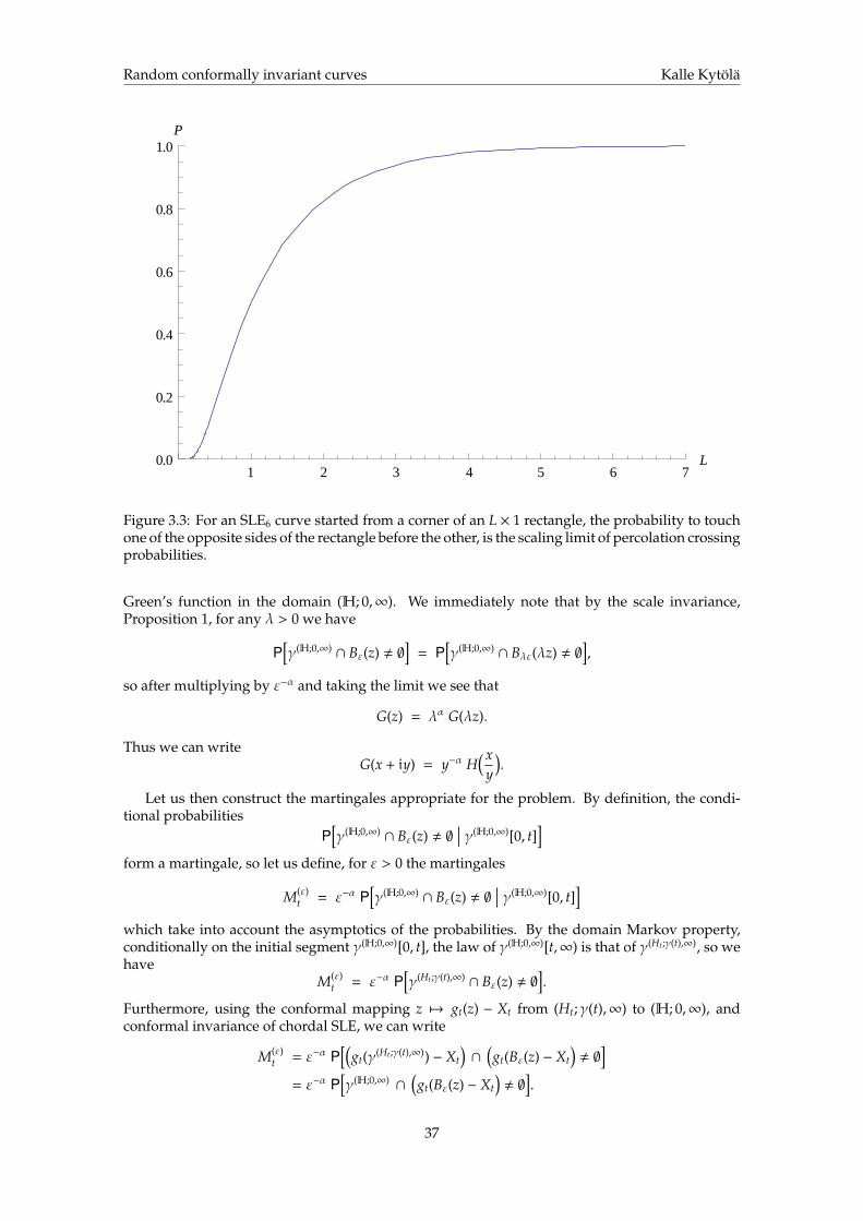
Random conformally invariant curves Kalle Kytola
1 2 3 4 5 6 7L0.0
0.2
0.4
0.6
0.8
1.0P
Figure 3.3: For an SLE6 curve started from a corner of an L × 1 rectangle, the probability to touchone of the opposite sides of the rectangle before the other, is the scaling limit of percolation crossingprobabilities.
Green’s function in the domain (H; 0,∞). We immediately note that by the scale invariance,Proposition 1, for any λ > 0 we have
P[γ(H;0,∞)
∩ Bε(z) , ∅]
= P[γ(H;0,∞)
∩ Bλε(λz) , ∅],
so after multiplying by ε−α and taking the limit we see that
G(z) = λα G(λz).
Thus we can writeG(x + iy) = y−α H
(xy
).
Let us then construct the martingales appropriate for the problem. By definition, the condi-tional probabilities
P[γ(H;0,∞)
∩ Bε(z) , ∅∣∣∣ γ(H;0,∞)[0, t]
]form a martingale, so let us define, for ε > 0 the martingales
M(ε)t = ε−α P
[γ(H;0,∞)
∩ Bε(z) , ∅∣∣∣ γ(H;0,∞)[0, t]
]which take into account the asymptotics of the probabilities. By the domain Markov property,conditionally on the initial segment γ(H;0,∞)[0, t], the law of γ(H;0,∞)[t,∞) is that of γ(Ht;γ(t),∞), so wehave
M(ε)t = ε−α P
[γ(Ht;γ(t),∞)
∩ Bε(z) , ∅].
Furthermore, using the conformal mapping z 7→ gt(z) − Xt from (Ht;γ(t),∞) to (H; 0,∞), andconformal invariance of chordal SLE, we can write
M(ε)t = ε−α P
[(gt(γ(Ht;γ(t),∞)) − Xt
)∩
(gt(Bε(z) − Xt
), ∅
]= ε−α P
[γ(H;0,∞)
∩
(gt(Bε(z) − Xt
), ∅
].
37

Random conformally invariant curves Kalle Kytola
Observe that the image of a small ball Bε(z) under a conformal map is approximately a small ballat the image point, with radius multiplied by the absolute value of the derivative of the map.Therefore we may write an approximation
M(ε)t ≈ ε−α P
[γ(H;0,∞)
∩ B|g′t(z)| ε(gt(z) − Xt)), ∅
],
which would in fact be an equality had we used an appropriate conformally invariant notion ofradius. Considering the limit ε 0 of the martingales, Mt = limε M(ε)
t , the approximation abovesays that the process
Mt = |g′t(z)|α G(gt(z) − Xt
)should be a local martigale. As before, we can now write the Ito derivative and obtain a differentialequation for G. Indeed, first note that Zt = gt(z) − Xt satisfies the (complex) Bessel type equation
dZt =2Zt
dt −√κ dBt,
or in terms of the real and imaginary parts Zt = Rt + i It
dRt =2Rt
R2t + I2
t
dt −√κ dBt, dIt =
−2It
R2t + I2
t
dt.
We also need the time derivative of |g′t(z)|, which is easiest to get in the logarithmic form: onereckognizes the derivative of the Loewner equation as
ddt
log(g′t(z)
)=
−2(gt(z) − Xt)2 ,
and then one takes the real part
d(
log |g′t(z)|)
=−2(R2
t − I2t )
(R2t + I2
t )2dt.
Taking into account the scale invariance G(x + iy) = y−α H(x/y) our local martingale reads
Mt =( |g′t(z)|
It
)αH(Rt
It
).
Applying Ito’s formula we get
dMt =8 |g′t(z)|α
I2+αt
(1 + r2
t
)−2 α H(rt) + (1 + r2
t ) rt H′(rt) +κ8
(1 + r2t )2 H′′(rt)
dt +
(· · ·
)dBt,
where we have denoted the ratio of real and imaginary parts by rt = RtIt
. Because the process is alocal martingale, the dt term has to vanish and therefore we require
α H(r) + (1 + r2) r H′(r) +κ8
(1 + r2)2 H′′(r) = 0.
Solutions to this differential equation exist for any α, and correspondingly there are local martin-gales of the desired form. However, the solution we are interested in should be positive. Once weobserve that the equation is an eigenvalue equation of Sturm-Liouville type, the eigenvalue being−α, and we recall that a positive solution must have the unique extremal eigenvalue, the numberα can be determined. We guess that the positive solution is of the form
H(r) = (1 + r2)β,
and then solve for β and α
β =κ − 82κ
, α = 1 −κ8.
38

Random conformally invariant curves Kalle Kytola
The result makes sense when α ≥ 0, that is, for κ ≤ 8.We in particular get the fractal dimension of the chordal SLEκ trace stated in Theorem ??
d = 2 − α = 1 +κ8,
and we have even found how the probability to visit small balls depends on the position of theball
P[γ(H;0,∞)
∩ Bε(x + i y) , ∅]∼
(εy
)1− κ8 1
(1 + x2
y2 )8−κ2κ
(3.2)
=(ε
y
)1− κ8(
sin(arg(x + i y))) 8−κ
κ .
Not surprisingly, for κ < 8, among balls whose center is at a given height y, the visiting probabilitygets smaller when the center of the ball gets further away from the starting point 0 of the SLEcurve. The limiting case κ = 8 suggests a constant probability to visit any ball, and indeed a morecareful analysis would show that the SLE trace then passes through any point almost surely.
39

Random conformally invariant curves Kalle Kytola
40

Bibliography
Lecture notes on SLE
[Bef10] V. Beffara: “Schramm-Loewner evolutions and other conformally invariant objects”. ClayMathematics Summer School, Buzios, Brazil (2010).
[Law10] G. Lawler: “Fractal and multifractal properties of SLE”. Clay Mathematics SummerSchool, Buzios, Brazil (2010).
[Wer02] W. Werner: “Random planar curves and Schramm-Loewner evolutions” Saint-Floursummer school (2002).
ICM talks related to SLEs
[Sch06] O. Schramm: “Conformally invariant scaling limits (an overview and a collection ofproblems)” ICM 2006.
[Smi06] S. Smirnov: “Towards conformal invariance of 2D lattice models” ICM 2006.
[Smi10] S. Smirnov: “Discrete Complex Analysis and Probability” ICM 2010.
Reviews on SLEs
[Car05] J. Cardy: “SLE for theoretical physicists”. Ann. Physics, 318, 81-118 (2005).
[KN04] W. Kager and B. Nienhuis: “A guide to stochastic Loewner evolution and applications”.J. Stat. Phys., 115, 1149-1229 (2004).
[BB06] M. Bauer and D. Bernard: “2D growth processes: SLE and Loewner chains”. Phys. Rep.,432, 115-222 (2006).
The textbook on SLE
[Law05] G. Lawler: “Conformally invariant processes in the plane”. American MathematicalSociety, 114 (2005).
Conformal mappings
[Ahl78] Ahlfors, L. V.: “Complex analysis”. McGraw-Hill Book Co., 1978.
[Ahl73] Ahlfors, L. V.: “Conformal invariants: topics in geometric function theory”. McGraw-HillBook Co., 1973.
41

Random conformally invariant curves Kalle Kytola
Stochastic calculus
[KS91] Karatzas, I. and Shreve, S. E.: “Brownian Motion and Stochastic Calculus”. Springer-Verlag, 1991.
[Oks02] Oksendal, B.: “Stochastic Differential Equations: An Introduction with Applications”-Springer, 2002.
[RY99] Revuz, D. and Yor, M.: “Continuous martingales and Brownian motion”. Springer-Verlag,1999.
The articles referred to in the text
[Bef08] V. Beffara, The dimension of the SLE curves. Ann. Probab. 36(4) 1421–1452 (2008).
[LSW04] G. Lawler, O. Schramm and W. Werner, Conformal invariance of planar loop-erasedrandom walks and uniform spanning trees. Ann. Probab., 32(1B), 939–995 (2004).
[RS05] S. Rohde and O. Schramm, Basic properties of SLE. Ann. Math., 161 (2), 883–924 (2005).
[Sch00] O. Schramm, Scaling limits of loop-erased random walks and uniform spanning trees.Israel J. Math., 118 221–288 (2000).
[SW05] O. Schramm and D. Wilson, SLE coordinate changes. New York J. Math., 11, 659–669(electronic) (2005).
[She09] S. Sheffield, Exploration trees and conformal loop ensembles. Duke Math. J., 147, 79–129(2009).
Kalle KytolaDepartment ofMathematics and Statistics
University of HelsinkiFinland
E-mail: [email protected]
42


![Rotation and Gray-Scale Transform-Invariant Texture ...the first-order or second-order statistics of textures [ 11-[8]. Later, Gaussian Markov random fields or Gibbs random fields](https://static.fdocuments.us/doc/165x107/5f1f74e2941b2b014e226d72/rotation-and-gray-scale-transform-invariant-texture-the-first-order-or-second-order.jpg)