Ramesh Melkote IJMTM Paper

This article was published in an Elsevier journal. The attached copyis furnished to the author for non-commercial research and

education use, including for instruction at the author’s institution,sharing with colleagues and providing to institution administration.

Other uses, including reproduction and distribution, or selling orlicensing copies, or posting to personal, institutional or third party

websites are prohibited.

In most cases authors are permitted to post their version of thearticle (e.g. in Word or Tex form) to their personal website orinstitutional repository. Authors requiring further information

regarding Elsevier’s archiving and manuscript policies areencouraged to visit:

http://www.elsevier.com/copyright

http://www.elsevier.com/copyright

Author's personal copy

International Journal of Machine Tools & Manufacture 48 (2008) 402–414

Modeling of white layer formation under thermally dominantconditions in orthogonal machining of hardened AISI 52100 steel

Anand Ramesh, Shreyes N. Melkote�

The George W. Woodruff School of Mechanical Engineering, Georgia Institute of Technology, Atlanta, GA, USA

Received 20 December 2006; received in revised form 15 September 2007; accepted 24 September 2007

Available online 6 October 2007

Abstract

This paper presents a finite element model for white layer formation in orthogonal machining of hardened AISI 52100 steel under

thermally dominant cutting conditions that promote martensitic phase transformations. The model explicitly accounts for the effects of

stress and strain, transformation plasticity and the effect of volume expansion accompanying phase transformation on the

transformation temperature. Model predictions of white layer depth are found to be in agreement with experimental values. The

paper also analyzes the effect of white layer formation on residual stress evolution in orthogonal cutting of AISI 52100 hardened steel.

Model simulations show that white layer formation does have a significant impact on the magnitude of surface residual stress and on the

location of the peak compressive residual stress.

r 2007 Elsevier Ltd. All rights reserved.

Keywords: Finite element modeling; White layer formation; Phase transformation; Hard machining; Orthogonal cutting

1. Introduction

Considerable attention has been focused in recent yearson understanding microstructure changes observed in thesurface layers of machined hardened steels. The micro-structure change is commonly referred to as white layer orwhite etching layer since it appears white when observed inan optical microscope after standard metallographicpreparation [1]. The layer is typically a few microns thickand is hard and brittle [2,3]. Due to common belief that thislayer is detrimental to fatigue life of the part, currentindustry practice is to superfinish the machined surface toremove the white layer. Alternatively, it is desirable todevelop a model capable of predicting the onset of whitelayer formation as a function of the machining conditions.Such a model can then be used to identify cuttingconditions that will not result in white layer or willproduce minimal white layer.

Over the years, a number of experimental investigationsaimed at understanding the formation mechanisms and

properties of white layer in machining and grinding havebeen reported [4–17]. However, very limited work has beenreported on modeling of white layer formation in machin-ing of hardened steels. Modeling of hard machining isincomplete without white layer formation because of itspossible effect on the evolution of residual stresses in themachined part surface.Although work on modeling of the hard turning process

to predict forces [18], chip formation [19,20] and tool wear[21] has been reported, only a handful of researchers haveattempted to explicitly model white layer formation inmachining and/or grinding of hardened steels. Mahdi andZhang [22–24] utilized a finite element (FE) framework topredict phase transformations in grinding. Akcan [25] andChou and Evans [26] used an analytical approach topredict white layer formation by solving a moving heatsource problem. These efforts assumed that white layerformation is due to thermally driven phase transformationeffects. However, they did not consider the mechanicaleffects of stress and strain on transformation temperatures,effect of volume expansion and transformation plasti-city associated with martensitic transformation andthe impact of white layer formation on residual stresses.

ARTICLE IN PRESS

www.elsevier.com/locate/ijmactool

0890-6955/$ - see front matter r 2007 Elsevier Ltd. All rights reserved.

doi:10.1016/j.ijmachtools.2007.09.007

�Corresponding author.

E-mail address: [email protected] (S.N. Melkote).


The importance of including these effects in the simulationof hard machining is discussed below.

Phase transformation in steel is accompanied by effectssuch as transformation plasticity and volume expansion.Transformation plasticity is an apparent increase inductility accompanying austenite–martensite transforma-tion in steels, while the volume expansion corresponds to a4.4% volume increase associated with martensite forma-tion [27,28]. This apparent increase in ductility has beenexplained as a pseudo-plasticity effect that arises from thechange in material yield stress over the transformationtemperature range [29]. The improvement in ductility dueto transformation plasticity is important in machining sinceit translates to increased strain, which in turn affects theflow stress. Improved ductility at high deformation ratesalso refines the grain size, further modifying the materialproperties. These effects are routinely incorporated in heattreatment simulations of steels [29–34] but have not beenincluded in models of white layer formation in machining.

It is known that defects such as dislocations act asnucleation sites for martensite. This suggests that deforma-tion of the material is beneficial to martensite transforma-tion [27]. Externally applied stress also increases thenumber of nucleation sites due to dislocation formationthereby assisting phase transformation [35]. Specifically,tensile deformation increases the martensite start (Ms)temperature, while shear deformation assists transforma-tion, martensite formation itself being a shear process [36].Such effects have not been considered in models of whitelayer formation in machining of hardened steels.

Another factor that has not been considered is the closerelationship that exists between phase transformations andthe resulting stress–strain evolution in the machinedsurface. Therefore, simulations of residual stress in theworkpiece are incomplete without the effects of white layerformation.

This paper presents an FE model of white layerformation in orthogonal machining of AISI 52100 har-dened steel that incorporates the effects of stress and strainon transformation temperature, volume expansion andtransformation plasticity. The model is valid for contin-uous white layer formation under thermally dominantcutting conditions where phase transformation is likely tooccur. Comparisons of model predictions with experimen-tal data are presented and the results discussed.

2. Development of thermo-mechanical FE model

The white layer model development in this paperemploys an FE-based thermo-mechanical model formula-tion of the orthogonal machining process.

The explicit dynamics FE procedure is used to developthe thermo-mechanical model of orthogonal cutting.ABAQUSs/Explicit v6.2 is used for all FE simulationsreported in this paper. Plane strain four-node quadrilateralelements of type CPE4RT are used to model the workpiece(AISI 52100, 62 HRC) and the tool (cBN). The workpiece

is modeled as elastic–plastic, whereas the tool is modeled aspurely elastic.The flow stress characteristics of the workpiece material

are modeled by the Johnson–Cook equation [37]. Thecoefficients of the flow stress equation were developedusing the procedure outlined by Shatla et al. [38]. Thenominal chemical composition and physical propertiesof the workpiece and tool materials used are given inTables 1–3, respectively.In order to aid the initial progress of the simulation, the

orientations of elements in the chip prior to the start ofmachining are altered as shown in Fig. 1 through the use ofBezier curves [39]. As can be seen, the basic shape of thechip is not changed. Only the configuration of the elementswithin the chip is altered.The boundary conditions imposed on the model are

shown in Fig. 2. The nodes along the left (AB), bottom(BC) and right side (CD) of the workpiece are constrainedagainst movement in the y-direction. They are given a

ARTICLE IN PRESS

Table 1

Nominal chemical composition of AISI 52100 steel (Metals Handbook,

1990)

Element C Cr Fe Mn Si P S

% Vol. 0.98–1.1 1.4 97.05 0.35 0.25 o0.25 o0.25

Table 2

Physical properties of workpiece material (AISI 52100, 62 HRC)

Density (kg/m3) 7827

Specific heat (J/kg 1C) 458, 25oTo204

640, 204oTo426

745, 426oTo537

798, T4537

Thermal conductivity (W/mK) 46.6

Coefficient of thermal expansion (/1C, � 10�6) 11.5, 25oTo204

12.6, 204oTo398

13.7, 698oTo704

14.9, 704oTo804

15.3, T4804

Young’s modulus (GPa) 210

Poisson’s ratio 0.277

Johnson–Cook constants

A (Mpa) 688.17

B (Mpa) 150.82

n 0.3362

C 0.04279

m 2.7786

Table 3

Physical properties of Kennametal KD120 grade cBN


Specific Heat (J/kg 1C) 750

Thermal conductivity (W/mK) 100

Coefficient of thermal expansion (/1C, � 10�6) 4.9



A. Ramesh, S.N. Melkote / International Journal of Machine Tools & Manufacture 48 (2008) 402–414 403


velocity in the x-direction equal to the cutting speed. Thenodes on the top and right side of the tool, denoted by MNand NO, are constrained in all directions. An initialtemperature of 25 1C is applied to all nodes in the model.Automatic time increment is used for the solutionprocedure. The model is solved via a fully coupledthermo-mechanical simulation.

The effective plastic strain criterion was used for thesimulation of chip formation. A baseline value is obtainedfrom the formula proposed by Guo and Dornfeld [40]:

�plf ¼2 cos aeffiffiffi

3pð1þ sin aeÞ

, (1)

where ae is the rake angle of the tool.For the cutting geometry used in this study, a value of

1.15 is obtained as a baseline value for the effective plasticstrain for chip formation. In reality, the effective plasticstrain at failure varies with strain, strain rate andtemperature, all of which vary with cutting conditions.Therefore, the sensitivity of model prediction to the valueof the effective plastic strain was evaluated via modelsimulations carried out at a cutting speed of 122m/min,

undeformed chip thickness (feed) of 0.127mm, 1mm widthof cut and 01 rake angle. In these simulations, the behaviorof the FE mesh around the tool edge and the forcepredictions was examined by varying the effective plasticstrain for failure over a range of values [41]. From thisanalysis, a value of 1.15 was found to work well for feedsless than 0.152mm while a value of 1.25 was found to workwell for feeds greater 0.152mm. This is attributed to thevariation of �plf with strain, strain rate and temperature, aswould occur with a change in feed. Note that Eq. (1) doesnot capture this probable variation.All tool–workpiece frictional interactions are modeled

using the Coulomb friction model, which is statedmathematically as

t ¼ ms when msotcrit ðslidingÞ,

t ¼ tcrit when ms ¼ tcrit ðstickingÞ, (2)

where t is the frictional shear stress, m is the coefficient offriction, s is the frictional normal stress and tcrit is theshear flow stress of the workpiece material and is equal to

tcrit ¼ sy=ffiffiffi3p

, (3)

where sy is the uniaxial flow stress of the material.As shown elsewhere [41], suitable values for tcrit were

obtained from Oxley’s predictive machining theory. Sensi-tivity studies were performed on this parameter and thecoefficient of friction (m). It is found that using the valuespredicted by Oxley’s method for tcrit and using m ¼ 0.35yield the best results.It is assumed that 90% of the energy expended during

plastic deformation is converted into heat. Also, frictionalheating is accounted for, with all the frictional energydissipated as heat.A mesh convergence study was also performed. It was

found that a coarse mesh (element length ¼ 25 mm) sufficedfor force predictions, but temperatures and plastic strainsbelow the workpiece surface converged to higher values foran element size of 3.125 mm. Validation of the flow stressequation was therefore carried out using the 25 mm mesh,

ARTICLE IN PRESS

Fig. 1. Modified region of chip to aid simulation progress.

Fig. 2. Boundary conditions in FE model.

A. Ramesh, S.N. Melkote / International Journal of Machine Tools & Manufacture 48 (2008) 402–414404


while modeling of white layer formation and residualstresses was carried out using the 3.125 mm mesh.

3. Thermo-mechanical model validation

Experimental validation of the thermo-mechanical FEmodel was carried out at this stage. Dry orthogonal cuttingtests were performed on a 25mm long and 0.9mm thicktube of hardened 52100 steel (62 HRC) on a two-axis CNClathe (Hardinge T42SP). A schematic of the test config-uration is shown in Fig. 3. As seen in the figure, the tool isfed axially into the tube with the cutting edge of the toolkept perpendicular to the feed and velocity vectors. High-cBN-content inserts (Kennametal NG3125R KD120grade) with nominally up-sharp edges were used with a01 rake angle tool holder (Kennametal NER 123B NF1).The length of each cut was fixed at 6.35mm.

ARTICLE IN PRESS

Cutting Forces

0

100

200

300

400

500

600

121.92 m/min,

0.152 mm/rev

152.4 m/min,

0.127 mm/rev

152.4 m/min,

0.152 mm/rev

152.4 m/min,

0.178 mm/rev

Machining Conditions: Cutting Speed/Feed

121.92 m/min,

0.152 mm/rev

152.4 m/min,

0.127 mm/rev

152.4 m/min,

0.152 mm/rev

152.4 m/min,

0.178 mm/rev

Machining Conditions: Cutting Speed/Feed

Cu

ttin

g F

orc

e,

N

Fc, Experiment

Fc, Oxley

Fc, FEM

Thrust Forces

0

50

100

150

200

250

300

350

Th

rust

Fo

rce,

N

Ft, Experiment

Ft, Oxley

Ft, FEM

Fig. 4. Comparison of predicted and experimental forces. All forces are in N per mm width of cut. Error bars denote the range of measured forces.

Table 4

Simulation conditions for thermo-mechanical FE model validation

Test no. Speed (m/min) Feed (mm) tcrit (Mpa) ef

1 121.92 0.152 578.46 1.15

2 152.4 0.127 580.87 1.15

3 152.4 0.152 566.34 1.15

4 152.4 0.178 554.37 1.25

Fig. 3. Schematic diagram of orthogonal cutting tests carried out on a

two-axis CNC lathe.



The cutting conditions used in the tests are shown inTable 4. The same conditions are used in the modelsimulations along with the values of tcrit and failure strainef. The value of coefficient of friction used for all conditionslisted in the table was 0.35. A 1mm width of cutwas simulated in all cases. Each cutting test was repeatedthree times and the cutting and thrust forces were measuredby a platform-type piezoelectric force dynamometer(Kistler 9257B).

A comparison of experimentally determined forces andpredicted values is shown in Fig. 4. It can be seen thatsatisfactory correlation is obtained between the experi-mental and predicted values. The maximum predictionerror in the cutting force is under 3% while the maximum

prediction error in the thrust force is about 13%. Thedeformed mesh configuration and temperature contours atthe end of a typical simulation are shown in Fig. 5.Based on the above results, the thermo-mechanical FE

procedure is deemed to be satisfactory for incorporatingthe phase transformation model of white layer formation,which is discussed next.

4. Modeling of white layer formation

Since the formation of white layers in hard machiningunder thermally dominant machining conditions conduciveto the occurrence of phase transformation is to be carried

ARTICLE IN PRESS

Fig. 5. Temperature contours and deformed configuration for 152.4m/min machining speed, 0.178mm feed validation case.



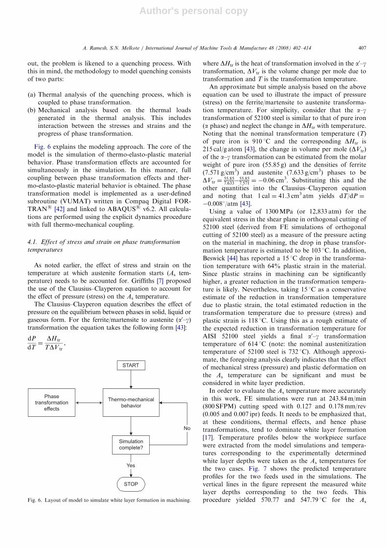
out, the problem is likened to a quenching process. Withthis in mind, the methodology to model quenching consistsof two parts:

(a) Thermal analysis of the quenching process, which iscoupled to phase transformation.

(b) Mechanical analysis based on the thermal loadsgenerated in the thermal analysis. This includesinteraction between the stresses and strains and theprogress of phase transformation.

Fig. 6 explains the modeling approach. The core of themodel is the simulation of thermo-elasto-plastic materialbehavior. Phase transformation effects are accounted forsimultaneously in the simulation. In this manner, fullcoupling between phase transformation effects and ther-mo-elasto-plastic material behavior is obtained. The phasetransformation model is implemented as a user-definedsubroutine (VUMAT) written in Compaq Digital FOR-TRANs [42] and linked to ABAQUSs v6.2. All calcula-tions are performed using the explicit dynamics procedurewith full thermo-mechanical coupling.

4.1. Effect of stress and strain on phase transformation

temperatures

As noted earlier, the effect of stress and strain on thetemperature at which austenite formation starts (As tem-perature) needs to be accounted for. Griffiths [7] proposedthe use of the Clausius–Clayperon equation to account forthe effect of pressure (stress) on the As temperature.

The Clausius–Clayperon equation describes the effect ofpressure on the equilibrium between phases in solid, liquid orgaseous form. For the ferrite/martensite to austenite (a0–g)transformation the equation takes the following form [43]:

dP

dT¼

DH tr

TDV tr,

where DHtr is the heat of transformation involved in the a0–gtransformation, DVtr is the volume change per mole due totransformation and T is the transformation temperature.An approximate but simple analysis based on the above

equation can be used to illustrate the impact of pressure(stress) on the ferrite/martensite to austenite transforma-tion temperature. For simplicity, consider that the a–gtransformation of 52100 steel is similar to that of pure iron(a phase) and neglect the change in DHtr with temperature.Noting that the nominal transformation temperature (T)of pure iron is 910 1C and the corresponding DHtr is215 cal/g atom [43], the change in volume per mole (DVtr)of the a–g transformation can be estimated from the molarweight of pure iron (55.85 g) and the densities of ferrite(7.571 g/cm3) and austenite (7.633 g/cm3) phases to beDVtr ¼

55:857:633�

55:857:571 ¼ �0.06 cm

3. Substituting this and theother quantities into the Clausius–Clayperon equationand noting that 1 cal ¼ 41.3 cm3 atm yields dT/dP ¼

�0.0081/atm [43].Using a value of 1300MPa (or 12,833 atm) for the

equivalent stress in the shear plane in orthogonal cutting of52100 steel (derived from FE simulations of orthogonalcutting of 52100 steel) as a measure of the pressure actingon the material in machining, the drop in phase transfor-mation temperature is estimated to be 103 1C. In addition,Beswick [44] has reported a 15 1C drop in the transforma-tion temperature with 64% plastic strain in the material.Since plastic strains in machining can be significantlyhigher, a greater reduction in the transformation tempera-ture is likely. Nevertheless, taking 15 1C as a conservativeestimate of the reduction in transformation temperaturedue to plastic strain, the total estimated reduction in thetransformation temperature due to pressure (stress) andplastic strain is 118 1C. Using this as a rough estimate ofthe expected reduction in transformation temperature forAISI 52100 steel yields a final a0–g transformationtemperature of 614 1C (note: the nominal austenitizationtemperature of 52100 steel is 732 1C). Although approxi-mate, the foregoing analysis clearly indicates that the effectof mechanical stress (pressure) and plastic deformation onthe As temperature can be significant and must beconsidered in white layer prediction.In order to evaluate the As temperature more accurately

in this work, FE simulations were run at 243.84m/min(800 SFPM) cutting speed with 0.127 and 0.178mm/rev(0.005 and 0.007 ipr) feeds. It needs to be emphasized that,at these conditions, thermal effects, and hence phasetransformations, tend to dominate white layer formation[17]. Temperature profiles below the workpiece surfacewere extracted from the model simulations and tempera-tures corresponding to the experimentally determinedwhite layer depths were taken as the As temperatures forthe two cases. Fig. 7 shows the predicted temperatureprofiles for the two feeds used in the simulations. Thevertical lines in the figure represent the measured whitelayer depths corresponding to the two feeds. Thisprocedure yielded 570.77 and 547.79 1C for the As

ARTICLE IN PRESS

Thermo-mechanical

behavior

START

Simulation

complete?

Yes

STOP

Phase

transformation

effects

No

Fig. 6. Layout of model to simulate white layer formation in machining.



temperatures for the two cases. These values deviate fromthe value (614 1C) estimated from the foregoing simpleanalysis by 7% and 10.7%, respectively.

The nominal temperature at which martensite formationstarts is taken to be 131.44 1C [28]. However, the nominalMs temperature is affected by stress, which can be modeledas [29]

DMs ¼ Askk þ Bs, (4)

where DMs reflects the change in the Ms temperature and A

( ¼ 0.05) and B ( ¼ 0.033) are material constants.If the temperature of a material point being analyzed

exceeds the As temperature, it is assumed to be instanta-neously austenitized. The temperatures of all such ‘‘trans-formed’’ material points in the FE model are subsequentlymonitored to check for the possibility of martensiteformation. If the temperature falls below the correctedMs temperature, the fraction of martensite formed isdetermined from the following equation proposed byKoistinen and Marburger [45]:

Fm ¼ ½1� expð�lðMs � TÞÞ�, (5)

where Fm is the fraction of martensite formed, l is amaterial constant equal to 0.011 for most steels and T is theinstantaneous temperature.

Since the FE procedure is based on an incrementalmethod, the change in the amount of martensite formeddue to a drop in temperature dT is given as

dFm ¼ �l expð�lðMs � TÞÞdT . (6)

The quantity of martensite present at any givenincrement, provided the temperature is below Ms and ifaustenitization has taken place, is therefore

Fnewm ¼ Fold

m þ dFm, (7)

where Fnewm and Fold

m are the martensite fractions at the endand beginning of the increment, respectively.As discussed earlier, an increase in ductility of the

material due to transformation plasticity is observed.Transformation plasticity can be modeled as an additionalsource of strain in the material, whose evolution isdescribed as follows [29]:

d�TP ¼ 2KTPsð1� FmÞdFm, (8)

where d�TP is the effective transformation plasticity strain,s is the effective stress and KTP is a material constant equalto 5.08e�5.The component-wise transformation plasticity strains

may then be calculated as [29]

d�TPij ¼3

2

d�TP

s

� �Sij , (9)

where Sij are the components of the stress tensor.Martensite formation also includes a 4.4% increase in

volume. This may be taken into account as follows:

d�TFij ¼13ð0:044 dFmÞdij , (10)

ARTICLE IN PRESS

Table 6

Material properties of low-cBN-content tool


Specific heat (J/kg 1C) 750

Thermal conductivity (W/mK) 4.4

Coefficient of thermal expansion (/1C, � 10�6) 4.9



Fig. 8. Regions showing phase transformation during machining.

Fig. 7. Simulated temperature profiles below workpiece surface for

cutting speed of 243.84m/min.

Table 5

Conditions used for prediction of white layer formation

Speed (SFPM/m/min) Feed (ipr/mm/rev)

700/213.36 0.005/0.127

900/274.32 0.005/0.127

700/213.36 0.007/0.178

900/274.32 0.007/0.178



where d�TFij represents the volumetric strain due tomartensite formation and dij is the Kronecker delta.

In order to incorporate the phase transformationprocedure in the elasto-plastic material model developedearlier in the paper, the transformation plasticity strains

and the transformation strains described by Eqs. (9) and(10) need to be included in the strain summation equationfor the material as follows:

�elij ¼ �eloldij þ d�ij � d�plij � d�TPij � d�TFij . (11)

ARTICLE IN PRESS

White layer Dark layer

White layer Dark layer

White layer Dark layerWhite layer Dark layer

Fig. 9. White layers generated at: (a) 213.36m/min (700 SFPM), 0.127mm/rev (0.005 ipr), (b) 274.32m/min (900 SFPM), 0.178mm/rev (0.007 ipr),

(c) 213.36m/min (700 SFPM), 0.127mm/rev (0.005 ipr), (d) 274.32m/min (900 SFPM), 0.178mm/rev (0.007 ipr).

0

0.5

1

1.5

2

2.5

213/0.127 274/0.127 213/0.178 274/0.178

Speed (m/min) / Feed (mm/rev)

Wh

ite

La

ye

r T

hic

kn

es

s,

µm

Predicted (µm) Measured Avg. (µm)

Fig. 10. Comparison between experimental and predicted values of white layer thickness.



Eqs. (4)–(11) describe the procedure for the simulation ofphase transformation during machining of the steel. Itmust be noted that only diffusionless transformations,namely, martensite formation, are accounted for by theequations outlined above.

The conditions used for the simulation of white layerformation are shown in Table 5. The FE simulationprocedure is identical to that described earlier. A meshusing 3.125 mm long elements is used in order to maximizethe sensitivity to temperature changes along the workpiecesurface. The tool material is a low-cBN-content gradewhose properties are given in Table 6. Note that the toolwas modeled with a flank wear land width of 100 mm tomatch the conditions used in the model validationexperiments described in the following paragraphs.

The austenite and martensite contents were moni-tored using solution-dependent state variables definedin ABAQUSs. A sample plot showing the occurrenceof phase transformation (indicated in red) for the274.32m/min and 0.178mm/rev (900 SFPM/0.007 ipr) caseis shown in Fig. 8. The unshaded elements immediately infront of the tool are elements in the sacrificial layer used tomodel the chip separation region.

Dry orthogonal cutting tests (see Fig. 3) were carried outon a 0.9mm thick tube of hardened 52100 steel (62 HRC)on a two-axis CNC lathe (Hardinge Model T42SP) at theseconditions using low-cBN-content tools (KennametalNG3125L KD081) with artificially generated flank wearlands of approximately 100 mm. The lower thermalconductivity of this tool (compared to high cBN) helps inchanneling more heat into the chip-work region, therebypromoting white layer formation. At the high cuttingspeeds used in these tests, even a fresh tool rapidly developsa measurable flank wear, which contributes to frictionalheating of the workpiece surface and thereby white layerformation. A 01 rake angle tool holder (Kennametal NER123B NF1) was used in the tests. The workpiece wassectioned and samples from two locations along themachined length were polished and etched using standardmetallographic techniques.

For the purpose of measuring the white layer thickness,optical micrographs were generated at two locations persample at a magnification of 2000. The white layerthickness was measured at 40–50 locations per micrographand averaged. The measurement error was estimatedto be about 10%. The white layers generated at thedifferent machining conditions used in the tests are shownin Fig. 9. Note that the somewhat darker regionimmediately below the white layer in the micrographs isthe so-called ‘‘dark layer’’, which mainly consists oftempered martensite.

A comparison of experimentally determined white layerthickness and predicted values is shown in Fig. 10. Notethat the predictions were made via model simulations thataccounted for the 100 mm artificially ground flank wearused in the experiments. It can be seen from the figure thatbetter agreement between predicted and measured values of

white layer thickness is obtained at higher feeds. However,it is found that all predicted values lie within 1.5 times thestandard deviation of the measured thickness.One potential explanation for the difference between the

measured and predicted values of white layer thickness isthe error associated with the measurement technique.Another explanation is the mesh density near the work-piece surface. Simulations were run with a mesh height ofapproximately 0.75 mm near the workpiece surface. Furtherrefinement would possibly improve some of the predic-tions, but the computational cost would increase dispro-portionately.

ARTICLE IN PRESS

Fig. 11. Validation of residual stresses predicted by finite element

simulations of orthogonal cutting. Experiment conditions reported by

Guo [46]: 0.1016mm feed, 0.762mm depth of cut, �51 rake angle, 1.6mm

tool nose radius.



Cutting tool inserts typically have a nominal cutting edgeradius (or hone). Honed edges promote temperature rise atthe tool–work interface. This effect was not considered inthe FE simulations. Dynamic remeshing and rezoningtechniques, which should alleviate problems associatedwith mesh size and cutting edge geometry, should improvethe accuracy of the simulations. These features arecurrently unavailable in ABAQUSs v6.2.

5. Modeling of residual stresses

In order to track residual stress evolution in theworkpiece after machining, the following approach is used:

� Once the machining pass is completed, the workpiece isdecelerated to a full stop in approximately 5 ms.� The tool is then backed away from the workpiece to

ensure that no surfaces of the tool are in contact withthe workpiece. The tool is also brought to a completehalt.� All thermo-mechanical loads applied to the model are

then deleted and the workpiece is allowed to cool toroom temperature. This is achieved by specifying aconvection film coefficient along the workpiece bound-ary. It is found that a value of 1.5� 10�4 J/smm2K

worked well for all the machining conditions studied.A sink temperature of 298K (25 1C) is specified as theenvironment temperature. Model temperatures werefound to be in the vicinity of 300K (27 1C) after asimulation period of 1000 s.

In order to verify the accuracy of the solution procedure,results from FE simulations are compared against experi-mental data for nose turning of AISI 52100 steel (62 HRC)reported by Guo [46].The cutting conditions used in the three-dimensional

nose turning test reported in Guo’s work are as follows:106.68m/min, 0.762mm depth of cut and 0.1016mm/revfeed. The tool (BZN 8100) used in this test had a nominalrake angle of �51 and a clearance angle of 51. Since muchof the cutting in this test occurs around the tool nose, theundeformed chip thickness is non-uniform. Therefore, inorder to achieve a meaningful comparison between theresidual stress distribution predicted by the white layermodel presented in this paper and the data reported byGuo, an effective undeformed thickness value thataccounts for the effect of tool nose radius needs to bedetermined and used in the orthogonal FE simulationsof the residual stress. The effective undeformed chipthickness in nose turning was calculated using the

ARTICLE IN PRESS

Fig. 12. Effect of white layer formation on circumferential residual stress.



following equation [47]:

teff ¼dt

rn½cos�1ðrn � d=rnÞ þ sin�1ðt=2rnÞ�, (12)

where d is the depth of cut, t is the nominal undeformedchip thickness and rn is the tool nose radius. Usingd ¼ 0.762mm, t ¼ 0.1016mm and rn ¼ 1.6mm yields avalue of 0.046mm for the effective undeformed chipthickness. This value was used in the FE simulation ofresidual stress in orthogonal cutting of AISI 52100 steel.The width of cut in the simulation was equal to 0.762mm.

As seen in Fig. 11, a fairly good agreement is obtainedbetween the predicted and measured values of thecircumferential and axial residual stresses.

5.1. Effect of white layer formation on residual stresses

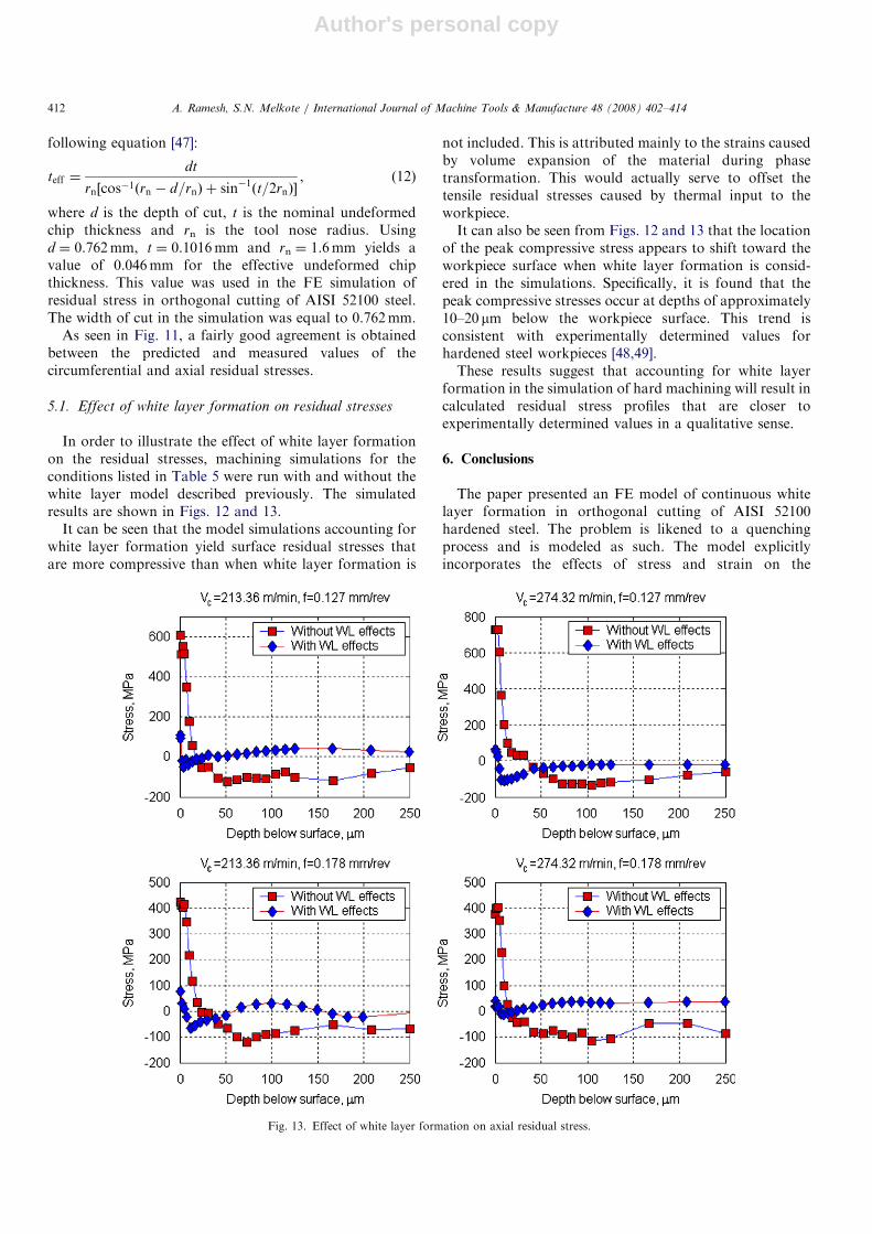
In order to illustrate the effect of white layer formationon the residual stresses, machining simulations for theconditions listed in Table 5 were run with and without thewhite layer model described previously. The simulatedresults are shown in Figs. 12 and 13.

It can be seen that the model simulations accounting forwhite layer formation yield surface residual stresses thatare more compressive than when white layer formation is

not included. This is attributed mainly to the strains causedby volume expansion of the material during phasetransformation. This would actually serve to offset thetensile residual stresses caused by thermal input to theworkpiece.It can also be seen from Figs. 12 and 13 that the location

of the peak compressive stress appears to shift toward theworkpiece surface when white layer formation is consid-ered in the simulations. Specifically, it is found that thepeak compressive stresses occur at depths of approximately10–20 mm below the workpiece surface. This trend isconsistent with experimentally determined values forhardened steel workpieces [48,49].These results suggest that accounting for white layer

formation in the simulation of hard machining will result incalculated residual stress profiles that are closer toexperimentally determined values in a qualitative sense.

6. Conclusions

The paper presented an FE model of continuous whitelayer formation in orthogonal cutting of AISI 52100hardened steel. The problem is likened to a quenchingprocess and is modeled as such. The model explicitlyincorporates the effects of stress and strain on the

ARTICLE IN PRESS

Fig. 13. Effect of white layer formation on axial residual stress.



transformation temperature, volume expansion and trans-formation plasticity and is valid for continuous white layerformation under thermally dominant cutting conditionswhere phase transformation is likely to occur. Experi-mental validation of the model is shown to yield predictedvalues and trends of white layer thickness that are in goodagreement with the measured values and trends.

It is found that accounting for white layer formation inthe model simulations results in more compressive surfaceresidual stress, which is explained by the volume expansionaccompanying the phase transformation. It is also foundthat accounting for white layer formation causes thelocation of the peak compressive stress to shift towardthe workpiece surface, as has been observed experimentallyby others [48,49].

Acknowledgments

This work was supported by a grant from the NationalScience Foundation (DMI-0100176). Additional supportwas provided by the NIST ATP Program (#70NAN-BOH3045). The authors are also grateful to the NationalCenter for Supercomputing Applications (NCSA) at theUniversity of Illinois at Urbana-Champaign for providingcomputer time for running the ABAQUS simulations.

References

[1] S. Akcan, S. Shah, S.P. Moylan, P.N. Chhabra, S. Chandrasekhar,

H.T.Y. Yang, Formation of white layers in steels by machining and

their characteristics, Metallurgical and Material Transactions A 33A

(2002) 1245–1254.

[2] A. Barbacki, M. Kawalec, Structural alterations in the surface layer

during hard machining, Journal of Materials Processing Technology

64 (1997) 33–39.

[3] A. Barbacki, M. Kawalec, A. Hamrol, Turning and grinding as a

source of microstructural changes in the surface layer of hardened

steel, Journal of Materials Processing Technology 133 (2003) 21–25.

[4] M. Field, J.F. Kahles, Review of surface integrity of machined

components, Annals of the CIRP 20 (2) (1971) 153–163.

[5] D.M. Turley, The nature of the white-etching layers produced during

reaming ultra-high strength steel, Materials Science and Engineering

19 (1975) 79–86.

[6] H. Eda, K. Kishi, S. Hashimoto, The formation mechanism of

ground white layers, Bulletin of the JSME 24 (190) (1981) 743–747.

[7] B.J. Griffiths, Mechanisms of white layer generation with reference to

machining and deformation processes, Transactions of the ASME:

Journal of Tribology 109 (1987) 525–530.

[8] H.K. Tonshoff, H.G. Wobker, D. Brandt, Hard turning—influences

on the workpiece properties, Transactions of NAMRI/SME XXIII

(1995) 215–220.

[9] A.M. Abrao, D.K. Aspinwall, The surface integrity of turned and

ground bearing steel, Wear 196 (1996) 215–220.

[10] E. Brinksmeier, T. Brockhoff, White layers in machining steels, in:

Proceedings of the Second International German and French

Conference on High Speed Machining, 1999, pp. 7–13.

[11] A. Vyas, M.C. Shaw, The significance of the white layer in a hard

turned steel chip, Machining Science and Technology 4 (1) (2000)

169–175.

[12] J.D. Thiele, S.N. Melkote, T.R. Watkins, R.A. Peascoe, Effect of

cutting edge geometry and workpiece hardness on surface residual

stresses in finish hard turning of AISI 52100 steel, Transactions of the

ASME, Journal of Manufacturing Science and Engineering 122 (4)

(2000) 642–649.

[13] J. Barry, J. Byrne, TEM study on the surface white layer in two

turned hardened steels, Materials Science and Engineering A 325

(2002) 356–364.

[14] X. Sauvage, J.M. Le Breton, A. Guillet, A. Meyer, J. Teillet, Phase

transformations in surface layers of machined steels investigated by

X-ray diffraction and Mossbauer spectrometry, Materials Science

and Engineering A 362 (2003) 181–186.

[15] V. Mahajan, Y.K. Chou, Machining-induced surface hardening due

to large wear land, Proceedings of the Institution of Mechanical

Engineers, Part B: Journal of Engineering Manufacture 218 (2004)

1647–1655.

[16] Y. Guo, J. Sahni, A comparative study of hard turned and

cylindrically ground white layers, International Journal of Machine

Tools and Manufacture 44 (2004) 135–145.

[17] A. Ramesh, S.N. Melkote, L.F. Allard, L. Riester, T.R. Watkins,

Analysis of white layers formed in hard turning of AISI 52100 steel,

Materials Science and Engineering A 390 (2004) 88–97.

[18] Y. Huang, S.Y. Liang, Modeling of cutting forces under hard turning

conditions considering tool wear effect, Transactions of the ASME,

Journal of Manufacturing Science and Engineering 127 (2) (2005)

262–270.

[19] Y.B. Guo, C.R. Liu, 3D FEA modeling of hard turning, Transactions

of the ASME, Journal of Manufacturing Science and Engineering 124

(2) (2002) 189–199.

[20] T.D. Marusich, R.J. McDaniel, S. Usui, J.A. Fleischmann, T.R.

Kurfess, S.Y. Liang, Three-dimensional finite element modeling of

hard turning processes, Proceedings of the ASME Manufacturing

Engineering Division—MED 14 (2003) 221–227.

[21] Y. Huang, T.G. Dawson, Tool crater wear depth modeling in cBN

hard turning, Wear 258 (9) (2005) 1455–1461.

[22] M. Mahdi, L. Zhang, Correlation between grinding conditions and

phase transformation of an alloy steel, in: L.C. Wrobel, et al. (Eds.),

Advanced Computational Methods in Heat Transfer III, Computa-

tional Mechanics Publications, Southampton, 1994, pp. 193–200.

[23] M. Mahdi, L. Zhang, Applied mechanics in grinding—VI. Residual

stresses and surface hardening by coupled thermo-plasticity and

phase transformation, International Journal of Machine Tools and

Manufacture 38 (1998) 1289–1304.

[24] M. Mahdi, L. Zhang, Applied mechanics in grinding. Part 7:

residual stresses induced by the full coupling of mechanical

deformation, thermal deformation and phase transformation, Inter-

national Journal of Machine Tools and Manufacture 39 (1999)

1285–1298.

[25] N.S. Akcan, Microstructure analysis and temperature modeling in

finish machining of hardened steels, M.S. Thesis, School of Industrial

Engineering, Purdue University, 1998.

[26] Y.K. Chou, C.J. Evans, White layers and thermal modeling of hard

turned surfaces, International Journal of Machine Tools and

Manufacture 39 (1999) 1863–1881.

[27] D.A. Porter, K.E. Easterling, Phase Transformations in Metals and

Alloys, Van Nostrand Reinhold, New York, 1981.

[28] G. Krauss, Steels: Heat Treatment and Processing Principles, ASM

International, Metals Park, OH, 1990.

[29] K.F. Wang, S. Chandrashekhar, H.T.Y. Yang, Experimental and

computational study of the quenching of carbon steel, Transactions

of the ASME, Journal of Manufacturing Science and Engineering 119

(1997) 257–265.

[30] F.G. Rammerstofer, D.F. Fischer, W. Mitter, K.J. Bathe, M.D.

Snyder, On thermo-elastic–plastic analysis of heat treatment pro-

cesses including creep and phase changes, Computers and Structures

13 (1981) 771–779.

[31] S. Denis, E. Gautier, A. Simon, G. Beck, Stress-phase transformation

interactions—basic principles, modelling, and calculation of internal

stresses, Materials Science and Technology 1 (1985) 805–814.

[32] S. Denis, S. Sjostrom, A. Simon, Coupled temperature, stress, phase

transformation calculation model numerical illustration of the

ARTICLE IN PRESSA. Ramesh, S.N. Melkote / International Journal of Machine Tools & Manufacture 48 (2008) 402–414 413


internal stresses evolution during cooling of a eutectoid carbon

steel cylinder, Metallurgical Transactions A 18A (1987)

1203–1212.

[33] S. Denis, E. Gautier, S. Sjostrom, A. Simon, Influence of stresses on

the kinetics of pearlitic transformation during continuous cooling,

Acta Metallurgica 35 (7) (1987) 1621–1632.

[34] K.F. Wang, S. Chandrashekhar, H.T.Y. Yang, An efficient 2-D finite

element procedure for the quenching analysis with phase change,

Transactions of the ASME, Journal of Engineering for Industry 115

(1993) 124–138.

[35] A.K. Jena, M.C. Chaturvedi, Phase Transformations in Materials,

Prentice-Hall, Englewood Cliffs, NJ, 1992.

[36] Z. Nishiyama, Martensitic Transformations, Academic Press,

New York, 1978.

[37] G.R. Johnson, W.H. Cook, in: Proceedings of the Seventh Interna-

tional Symposium on Ballistics, American Defence Preparedness

Association (ADPA), Netherlands, 1983.

[38] M. Shatla, C. Kerk, T. Altan, Process modeling in machining, part I:

determination of flow stress data, International Journal of Machine

Tools and Manufacture 41 (2001) 1511–1534.

[39] M. Baker, C. Siemers, J. Rosler, A finite element model of high speed

metal cutting with adiabatic shearing, Computers and Structures 80

(5–6) (2002) 495–513.

[40] Y.B. Guo, D.A. Dornfeld, Finite element modeling of burr formation

process in drilling 304 stainless steel, Journal of Manufacturing

Science and Engineering 122 (2000) 612–619.

[41] A. Ramesh, Prediction of process-induced residual stresses and

microstructural changes in orthogonal hard machining, Ph.D. Thesis,

Mechanical Engineering, Georgia Institute of Technology, 2002.

[42] R.L. Martineau, A viscoplastic model of expanding cylindrical shells

subjected to internal explosive detonations, Ph.D. Thesis, Depart-

ment of Mechanical Engineering, Colorado State University, Fort

Collins, CO, 1998.

[43] L.S. Darken, R.W. Gurry, Physical Chemistry of Metals, CBS Press,

New Delhi, 1953.

[44] J. Beswick, Effect of prior cold work on the martensite transforma-

tion in SAE 52100, Metallurgical Transactions 15A (1984) 299–306.

[45] D.P. Koistinen, R.E. Marburger, A general equation prescribing the

extent of the austenite–martensite transformation in pure iron carbon

alloys and carbon steels, Acta Metallurgica 7 (1959) 59.

[46] Y.B. Guo, 3-D modeling of superfinish hard turning, Ph.D. Thesis,

Department of Industrial Engineering, Purdue University, 2001.

[47] T.G. Dawson, Effects of cutting parameters and tool wear in hard

turning, Ph.D. Thesis, School of Mechanical Engineering, Georgia

Institute of Technology, 2002.

[48] E. Schreiber, H. Schlicht, Residual stresses after turning of hardened

components, in: G. Beck, S. Denis, A. Simon (Eds.), Proceedings of

the Second International Conference on Residual Stresses (ICRS 2),

Elsevier, New York, 1988, pp. 853–860.

[49] A. Ramesh, J.D. Thiele, S.N. Melkote, Residual stresses and subsurface

flow in finish hard turned AISI 4340 and 52100 steels: a comparative

study, Proceedings of the ASME IMECE, MED 10 (1999) 831–837.

ARTICLE IN PRESSA. Ramesh, S.N. Melkote / International Journal of Machine Tools & Manufacture 48 (2008) 402–414414

Ramesh Melkote IJMTM Paper

Documents

Transcript of Ramesh Melkote IJMTM Paper