
ONCE UPON A TIME… FIT CHALLENGE!. Jennifer Michelis FIT CHALLENGE CREATORS!

K.7
Raising an Inflation Target:
The Japanese Experience with Abenomics De Michelis, Andrea and Matteo Iacoviello
International Finance Discussion Papers Board of Governors of the Federal Reserve System
Number 1168 May 2016
Please cite paper as: De Michelis, Andrea and Matteo Iacoviello (2016). Raising an Inflation Target: The Japanese Experience with Abenomics International Finance Discussion Papers 1168.
http://dx.doi.org/10.17016/IFDP.2016.1168

Board of Governors of the Federal Reserve System
International Finance Discussion Papers
Number 1168
May 2016
Raising an Inflation Target:
the Japanese Experience with Abenomics
Andrea De Michelis and Matteo Iacoviello
NOTE: International Finance Discussion Papers are preliminary materials circulated to stimulatediscussion and critical comment. References to International Finance Discussion Papers (otherthan an acknowledgment that the writer has had access to unpublished material) should be clearedwith the author or authors. Recent IFDPs are available on the Web at www.federalreserve.
gov/pubs/ifdp/. This paper can be downloaded without charge from the Social Science ResearchNetwork electronic library at www.ssrn.com.
Raising an Inflation Target:
the Japanese Experience with Abenomics∗
Andrea De Michelis and Matteo Iacoviello†
Federal Reserve Board
May 26, 2016
This paper draws from Japan’s recent monetary experiment to examine the effects of an increase
in the inflation target during a liquidity trap. We review Japanese data and examine through a
VAR model how macroeconomic variables respond to an identified inflation target shock. We apply
these findings to calibrate the effect of a shock to the inflation target in a new-Keynesian DSGE
model of the Japanese economy. We argue that imperfect observability of the inflation target and
a separate exchange rate shock are needed to successfully account for the behavior of nominal and
real variables in Japan since late 2012. Our analysis indicates that Japan has made some progress
towards overcoming deflation, but further measures are needed to raise inflation to 2 percent in a
stable manner.
KEYWORDS: Abenomics, Credibility, Deflation, Inflation target, Japan, Monetary policy.
JEL CLASSIFICATION: E31, E32, E47, E52, E58, F31, F41
∗The views expressed in this paper are solely the responsibility of the authors and should not be interpreted asreflecting the views of the Board of Governors of the Federal Reserve System or of any other person associated withthe Federal Reserve System. Christopher Erceg gave us very useful advice at an early stage. We are also very gratefulto Keith Kuester for several helpful suggestions and comments. We thank Guido Ascari, Kosuke Aoki, GianlucaBenigno, Ikeda Daisuke, Luca Guerrieri, Jesper Linde, Steven Kamin, Robert Kollmann, Eric Leeper, Andrea Raffo,Werner Roeger, Andrea Tambalotti, Harald Uhlig as well as participants at “The Post-Slump Conference” in Brussels,at the Federal Reserve’s International Finance Workshop on “Spillovers from Accommodative Policies since the GlobalFinancial Crisis”, and at seminars at the European Central Bank, the Banque de France, and the Bank of Japanfor helpful comments and suggestions. We also thank Anders Warne for the Matlab code used to estimate the VARmodel. Katherine Marsten, Aaron Markiewitz and Rebecca Spavins provided excellent research assistance.
†Division of International Finance, Federal Reserve Board, 20th and C St. NW, Washington, DC 20551. E-mailaddresses: [email protected] (De Michelis) and [email protected] (Iacoviello)
2

1 Introduction
This paper studies the effects of an increase in the inflation target during a liquidity trap. To
this end, we discuss Japan’s recent aggressive monetary easing measures, including the adoption
of a 2 percent inflation target in early 2013, and review the behavior of prices and exchange rates
following this policy change. We then use a VAR to document that output and exchange rates
respond more to inflation target shocks when the economy is in a liquidity trap. Finally, we use
our empirical findings to calibrate two DSGE models of the Japanese economy that can account
for the sluggish behavior of nominal and real variables in response to an inflation target shock. An
important feature of our model is that agents update their estimates of the inflation target only
gradually over time. As a consequence, consistent with Japanese data since 2012, inflation and
inflation expectations rise very slowly after an increase in the target. Accordingly, changes in the
inflation target, while relatively powerful in a liquidity trap, can be weakened by the slow response
of inflation.
A wide economic literature has documented the Japanese malaise of low economic growth and
mild deflation, alongside high public debt and a rapidly aging population (e.g. Ito and Mishkin
2006). Figure 1 shows that Japanese inflation turned negative in the late 1990s. The emergence of
deflation is generally attributed to the failure of policies conducted by the Bank of Japan (BOJ).
Inflation is a monetary phenomenon, the argument goes, and the BOJ was unable to stop the
inflation rate from turning negative. Many observers, including Krugman (1998) and Bernanke,
Reinhart, and Sack (2004), have argued that the BOJ’s efforts were too little and too late, calling
for more aggressive and proactive measures. The aftermath of the global financial crisis provides a
case in point. The BOJ lowered its policy rate to zero and expanded the size of its balance sheet.
However, as deflation intensified, the BOJ came under criticism for the limited scope of its asset
purchase program and for lacking conviction that easing would yield tangible benefits.
Against this background, Mr. Shinzo Abe was elected Prime Minister in late 2012, running
on an economic platform known as “Abenomics.” Abenomics calls for ending Japan’s long slump
with three “arrows”: aggressive monetary easing; flexible fiscal policy; and structural reforms
(Eichengreen 2013, Ito 2013). Even before coming into power, Mr. Abe started calling for a radical
reorientation of monetary policy in November 2012. In February 2013, the BOJ introduced a
new inflation target of 2 percent, though it refrained from pursuing significantly more aggressive
easing. In April 2013, under the new leadership of Governor Haruhiko Kuroda, the BOJ unveiled
2

a new policy package entitled “Quantitative and Qualitative Monetary Easing” (QQE). The BOJ
announced a sharp increase in purchases of Japanese government bonds (JGBs) and other assets,
including Japanese equity ETFs. The BOJ also extended the maturity of its JGB purchases.
In October 2014, the BOJ expanded its QQE program by slightly accelerating the pace of asset
purchases. Figure 2 shows that the BOJ’s balance sheet has more than doubled in size since the
introduction of QQE. To provide a reference point, the increase in the BOJ’s asset-to-GDP ratio
since the start of QQE is roughly twice that of the Federal Reserve over the 6-year period from
2008 to 2014.
Has the first arrow of Abenomics hit its target? In this paper, we note that there has been
some progress, but that the goal has yet to be reached. Inflation has turned positive, ending a
15-year period of persistent deflation. Inflation expectations have moved up, however they remain
well below the 2 percent target, suggesting that private agents remain doubtful. Japan’s experience
raises the concern that expansionary monetary policies may not be effective unless they are fully
credible. To better assess the risks, benefits and challenges of raising an inflation target, we first
estimate the effects of an inflation target shock using a simple VAR and then analyze the monetary
regime change taking place under Abenomics through the prism of two new-Keynesian models
exhibiting inertial inflation behavior and imperfect credibility. Our main finding is that increasing
an inflation target can have powerful effects on activity and inflation, especially when the economy
is in a liquidity trap. However, we also show that these effects can be smaller if the policy is not
fully credible. Accordingly, we argue that the BOJ needs to take further steps to strengthen its
credibility by more effectively communicating the permanent nature of the monetary regime shift.
Our work is related to various strands of literature. First, our paper contributes to the literature
on Japanese unconventional monetary policy. Previous research has generally focused on the BOJ’s
asset purchases. For example, Rogers, Scotti, and Wright (2014) examine how asset prices are
affected by unconventional monetary policy announcements. A notable exception is the work of
Hausman and Wieland (2015) who argue that the monetary policy of the BOJ under Abenomics
provided a modest boost to Japanese output. We expand on this literature by laying out an
empirical modeling strategy to identify the effects of an inflation target shock and by investigating
the transmission channels of a higher inflation target in a general equilibrium framework.
Second, our empirical analysis draws from the estimation of VAR models through long–run
restrictions pioneered by Blanchard and Quah (1989), King, Plosser, Stock, and Watson (1991),
and Warne (1993). We find this methodology appealing for our purposes because it hews closely
3

to the notion of what shocks to the inflation target do – or, at least, should do –, which is to
change the inflation rate at very long horizons. In particular, the identification assumptions of
our inflation target shock mimics those of the neutral inflation shock in King, Plosser, Stock, and
Watson (1991): the shock affects inflation and nominal rates by the same amount in the long run,
and has no long–run effect on the real variables, including output. These restrictions, in particular,
are also shared by the DSGE models that we use throughout the paper.
Third, our modeling strategy and the focus on imperfect credibility of the monetary authority
build on Erceg and Levin (2003) and Ireland (2007). Our main intuition is that the challenges faced
by the BOJ to reflate the Japanese economy are the mirror image of those faced by the Federal
Reserve following the high inflation of the 1970s. Goodfriend and King (2005) have prominently
argued that the Volcker disinflation was complicated by the Federal Reserve’s imperfect credibility
in the aftermath of the high inflation of the 1970s. We believe that the Bank of Japan has been facing
similar, if not deeper, credibility issues given its long struggle with deflation. Following Erceg and
Levin (2003), we model the high degree of inflation persistence as the result of the private agents’
inability to disentangle transitory from persistent movements in the inflation target. We contribute
to this literature by investigating the effects of a change in the inflation target in a liquidity trap.
We show that, at the zero lower bound (ZLB), the lack of credibility increases inflation persistence
and dampens the output response. Intuitively, with the interest rate at the zero bound, a slower rise
in inflation leads to a smaller decrease in the real interest rate and to a smaller output expansion.
The remainder of the paper is organized as follows. Section 2 reviews how Japanese consumer
prices, trade prices, and exchange rates have evolved since the start of Abenomics. Section 3 sets
up a simple VAR model to examine what Japanese data over the past 40 years reveal about the
real effects of changing an inflation target. Section 4 presents a theoretical analysis of an inflation
target shock in a closed-economy, new-Keynesian DSGE model with inertial inflation behavior and
imperfect credibility. Section 5 extends the previous analysis to an open-economy environment
using the Federal Reserve staff’s SIGMA model. Section 6 concludes.
2 Reflation, Prices and Exchange Rates in the aftermath of Abenomics
We see the adoption of the 2 percent inflation target as the cornerstone of Abenomics. We do
not question here the optimality of this particular value. While several macroeconomic models
indicate optimal inflation rates close to zero, other considerations have induced most central banks
to prefer small but positive inflation rates. BOJ’s Governor Kuroda gave two reasons for adopting
4

a 2 percent target in Japan: mismeasurement of actual inflation, and risks of hitting the zero lower
bound when inflation is low (Kuroda 2013).
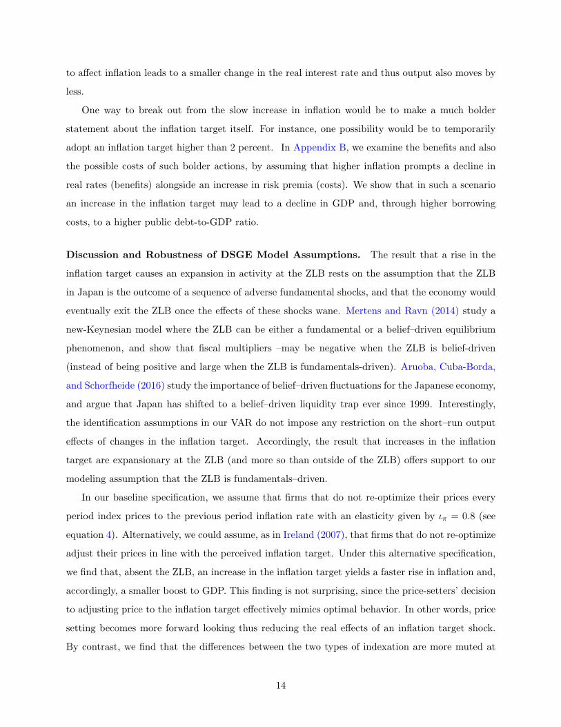
BOJ officials have appealed to a simple Phillips curve framework to justify why they need to
increase their inflation target. Figure 3 shows estimates of Japan’s Phillips curve, relating core
inflation (excluding food and energy prices) to a constant term and the output gap, over three
sample periods. Panel A is estimated over the full sample 1980Q1–2015Q2, Panel B over 1980Q1–
1993Q4, and Panel C over 1994Q1–2013Q2, with B and C corresponding to the high and low
inflation periods, respectively. Comparing Panel B with Panel C, the Phillips curve appears to
have shifted down. The intercept term has fallen from 2.5 percent in the earlier period to 0 percent
in the later period. Loosely speaking, the intercept identifies the steady-state rate of inflation
that is obtained when the output gap is closed. Accordingly, merely closing the gap might not be
sufficient to raise inflation to 2 percent. Indeed, the estimated Phillips curve appears so flat that
raising inflation to 2 percent would require an implausibly high output gap. Rather, the actions
of the BOJ under Abenomics are aimed at shifting up the Phillips curve by resetting inflation
expectations to a higher value, as argued by BOJ’s policy board member Shirai (2013).
How much did inflation rise following the start of Abenomics? As shown in Figure 1, total
inflation has moved from −0.4 percent in the third quarter of 2012 to 0.4 percent in the second
quarter of 2015 and core inflation from −0.6 percent to 0.4 percent. Both measures of inflation
moved up sharply early on, rising well above 2 percent in 2014; however, a large component of
this run-up reflected transitory factors. First, the yen depreciated more than 30 percent between
mid-2012 and 2015, boosting import prices and, in turn, consumer prices (see Figure 4). A simple
bivariate regression of total inflation on import price inflation attributes half of the 2013 increase in
inflation to higher import prices.1 Second, the consumption tax rate was raised from 5 to 8 percent
in April 2014, pushing up inflation by about 2 percentage points that year. Taken together, the
evidence seems to indicate that the policies of the BOJ under Abenomics have thus far moved up
underlying domestic inflation by about 1 percentage point.
Inflation expectations have also moved up, but they remain well below the 2 percent target. As
noted in (Mandel and Barnes 2013), there is no ideal measure of inflation expectations in Japan.2
1 We run a simple regression of total inflation on import price inflation and the output gap over the period 1992Q1-2012Q4. The regression results suggest that, over the 2012Q3–2014Q1 period, a 23 percent rise in import prices added0.7 percentage point to total inflation. This estimate likely provides a lower bound as imports of fossil fuels jumpedup after Japan shut down its nuclear reactors following the nuclear disaster in March 2011, arguably contributing torender Japan consumer prices more sensitive to exchange rate fluctuations.
2 Measures derived from financial markets suffer from the lack of sufficient liquidity. In particular, breakeven
5

That said, in Table 1, we report some of the available measures of inflation expectations before
and after the advent of Abenomics. Here we focus on longer-term inflation expectations because
we want to assess the BOJ’s progress towards its goal of raising inflation to 2 percent “in a stable
manner.” As is also shown in Figure 5, the 5 × 5 swap rate (a measure of inflation compensation
6 − 10 year ahead) has increased from 0 percent in mid-2012 to 1.2 percent in mid-2015, whereas
6 − 10 year ahead inflation forecasts by Consensus have moved up by 0.8 percentage point. In
addition, 10–year JGB yields have remained very low, trading near 50 basis points in 2015, and
10–year forward rates are barely above 1 percent even at the end of 2018 suggesting that inflation
risk premia have remained very low (Figure 6). In sum, we read the available evidence as indicating
that Japanese longer-term inflation expectations have risen by only 1 percentage point since the
start of Abenomics and remain well below the new 2 percent inflation target of the Bank of Japan.
Table 1: Japanese Longer-Term Inflation Expectations (percent)
5x5 inflation 10-year inflation 6-10 year ahead 2-6 year aheadswap rate swap rate inflation by Consensus inflation by EPS
2012 Q3 0.0 0.3 0.8 0.4
2015 Q2 1.2 1.0 1.6 1.3
change (ppt) 1.2 0.7 0.8 0.9
Sources: Bloomberg, Consensus Economics, and Japanese Center for Economic Research.
3 VAR Evidence
Do changes in the inflation target produce real effects? Ideally, one would like to identify in the
data exogenous movements in the inflation objective of the central bank that are uncorrelated with
other developments in the economy. In practice, such movements almost never occur. We then
proceed by adopting an operational definition of what a change in the inflation target should do.
Building on the methodology developed by King, Plosser, Stock, and Watson (1991) and Warne
(1993), we formulate a 5–variable vector error correction model with core inflation, bank’s lending
inflation measures are not reliable because the market for inflation-linked Japanese government bonds is very thinand a majority of the issuance has been bought back by the Ministry of Finance in recent years. Short-term measures ofinflation expectations from surveys of households, investors, and professional forecasters appear to be more responsiveto actual inflation than predictive of the future. Longer-term measures, such as the 6−10 year ahead inflation forecastsby Consensus, performed poorly over the past two decades, remaining close to 1 percent despite the emergence ofpersistent deflation.
6

interest rate, real exchange rate, GDP, and real oil prices.3 The model is estimated using Japanese
quarterly data since 1974. We measure inflation with core CPI inflation (excluding energy and
food prices). We use such measure (rather than total CPI inflation) because a smoother measure of
underlying inflation is more suitable to identify changes in the inflation target. We measure interest
rates using the average lending rate charged by large Japanese banks.4 We measure exchange rates
using the trade-weighted real exchange rate published by the BIS. We measure GDP using the
official Cabinet Office estimate of the output gap, a measure of the cyclical component of GDP
akin to the CBO’s output gap for the United States.5 For oil prices, we use the WTI price of oil
deflated by U.S. CPI inflation.6
We identify shocks to the inflation target as follows. We impose the restriction that a change
in the inflation target (1) affects inflation and the interest rate by the same amount (percentage-
wise) in the long-run, but (2) has no long-run effect on GDP, the real exchange rate, and real oil
price inflation. These restrictions might appear draconian, but are implied by nearly all modern
monetary business cycle models. We also assume that Japanese inflation has no contemporaneous
effect on oil prices given that the price of oil is determined by global rather than Japanese-specific
developments.7
Figure 7 plots the impulse responses of inflation, interest rate, exchange rate, and GDP to the
identified inflation target shock for the VAR estimated over two subperiods, 1974Q1-1993Q4 and
1994Q1-2015Q2.8 We choose these two samples to account for the different effects of inflation target
shocks depending on whether the economy is in a liquidity trap or not. As noted earlier, 1994 is
3 We control for oil prices in the VAR to better account for cost–push factors that can drive inflation dynamics.4 We use the lending rate rather that government bond yields because of data availability. The series on the 10-year
JGB yield published by the Ministry of Finance starts in 1986 whereas the bank lending rate is available since 1965.Since 1986, the two series move in synch, with a correlation of 0.97.
5 Alternatively, we detrended real GDP using a band-pass filter and obtained similar results.6 All series were drawn from Haver Analytics. Core inflation is the four-quarter change in the consumer price
level, excluding food and energy prices (Haver series mnemonic: H158PCXG@G10) and net of the effects of theconsumption tax hikes of 1989Q2, 1997Q2, and 2014Q2. GDP is the Cabinet’s Office output gap (Haver seriesmnemonic: JPGDPG@JAPAN). The real exchange rate is the Trade Weighted Real Effective Foreign ExchangeRate (EERBR@JAPAN). The interest rate is the Average Lending Rate by City Banks (AICG@JAPAN) on loansand discounts with maturity of less than one year at the time of origination. Oil price inflation is the 4-quartergrowth rate of WTI (PZTEXP@USECON) minus U.S. CPI 4-quarter inflation (PCUN@USECON).
7 Our VAR model takes the form of a restricted vector error correction model. The restriction that we impose isthat (1) the output gap, (2) the log real exchange rate, (3) oil price inflation and (4) the difference between nominalinterest rate and inflation are all stationary variables. In turn, these four restrictions allow us to decompose thestructural shocks into four transitory shocks and one permanent shock. The latter is the only source of the commonstochastic trend between nominal interest rate and inflation.
8 The response of the oil price (not shown in the figure) to the inflation target shock is modest and not significantlydifferent from zero at all horizons.
7

when the low inflation period starts, with core inflation falling persistently below 1 percent.
For ease of comparability across subperiods, we scale the size of the shock and of the responses
so that in both samples the eventual rise in inflation is 2 percentage points, on average. Such
scaling is inconsequential as the underlying VAR is linear in its coefficients. The rescaled shock
corresponds to a 3–standard deviation shock in the early sample, when inflation in Japan was
high and volatile, and, perhaps unsurprisingly, to a larger, 6–standard deviation shock in the late
sample, when inflation was low and relatively stable. In both periods, the identified inflation target
shock leads to a gradual and permanent increase in inflation and the nominal interest rate, and to
a temporary boost in output. By construction, GDP as well as the real exchange rate return to
their initial baseline in the long run.
The comparison between the two periods reveals important differences. In the early period,
the identified inflation target shock leads to a temporary rise in real interest rates, as the nominal
interest rate rises faster than inflation. In turn, higher real rates lead to a real appreciation, and
thus GDP rises only slightly above its baseline. In the late sample, perhaps because short-term
interest rates are effectively at zero, the response of the lending rate is more subdued in spite of
the more front-loaded increase in the inflation rate. Accordingly, the real rate declines. In contrast
with the early period, the real exchange rate depreciates substantially and persistently. In line
with these findings, the boost to GDP is substantially larger in the late sample. To give some
quantitative flavor, a 2 percentage point increase in the target leads to a rise in GDP of only 0.3
percent in the early sample and almost 4 percent in the late sample.
The results from the VAR analysis indicate that reflating the economy can bring substantial
short-run benefits in terms of output when the economy is in a liquidity trap. However, taken at
face value, this analysis also suggests the Bank of Japan needs to produce an inflation shock that
is 6 standard deviations above its mean over the last 20 years. This is a formidable challenge,
especially in an environment where private agents might take only limited signal from movements
in interest rates, which at shorter maturities remain constrained by the zero lower bound.
Later in the paper, we confirm the plausibility of our identification scheme in two ways. First,
we confirm in Section 4, through a series of Monte Carlo experiments, that our identification scheme
retrieves the true impulse responses of a DSGE model when applied to artificial data generated by
the model itself. Second, and more prosaically, we show in Appendix A analogous results from a
VAR applied to U.S. data. Such exercise also shows that a rise in the inflation target can lead to
a short-run increase in output.
8

VAR’s Historical Decomposition. The estimated VAR can be used to quantify the extent to
which the rise in the inflation target has effectively moved inflation and the real exchange rate. To
address this question, we carry out a historical decomposition of inflation into the shocks identified
by our model.
The top panel of Figure 8 plots the contribution over time of the inflation target shock to the
behavior of core inflation since 2010. The panel shows that the inflation target shock identified by
the model has added at most 0.8 percentage point to core inflation since the start of Abenomics
in 2013Q4. Is such an increase unprecedented? The impulse responses indicate that a typical one-
standard deviation shock to the target in the late sample would raise inflation by approximately
0.25 percentage point after three years. Accordingly, the Abenomics shock to the inflation target
was at most 3 standard deviations, about half as much as plotted in the bottom panels of Figure
7. However, considerable uncertainty surrounds this estimate. If we move the start of Abenomics
to early 2013, when the BOJ began to implement actual policy steps, the size of shock would be
about half as large. In addition, even prior to Abenomics, the historical decomposition reveals that
the contribution of the inflation target shock was positive, perhaps reflecting earlier attempts by
the BOJ to escape deflation. All told, these considerations suggest that the BOJ under Abenomics
has taken important steps, but not enough to engineer a clear discontinuity with the past.
Similarly, the bottom panel of Figure 8 plots the contribution of the inflation target shock to
the real exchange rate. This decomposition shows that the inflation target shock identified by the
VAR has led to a real exchange rate depreciation of less than 6 percent. The contribution of the
shock is relatively small, accounting for only one-fifth of the 30 percent depreciation of the yen
since the start of Abenomics.
Summing up, the VAR analysis indicates that the BOJ under Abenomics has raised trend
inflation only partially toward its new 2 percent target, confirming the findings of Section 2. Fur-
thermore, the inflation target shock of Abenomics appears to have only modestly contributed to
the depreciation of the yen.
4 A Closed Economy New-Keynesian Model
Section 3 showed how Japanese macroeconomic variables respond to identified inflation target
shocks. We now continue our investigation by examining the effect of inflation target shocks
in a standard closed economy new-Keynesian model. The model, a variant of a small-scale DSGE
model in the tradition of Christiano, Eichenbaum, and Evans (2005) and Smets and Wouters (2007),
9

features Calvo-style nominal price and wage rigidities, habit formation in consumption, investment
adjustment costs, a fiscal authority, and a central bank that follows an interest rate rule subject to
the zero lower bound. In most respects, the calibration of the model closely follows the estimated
parameters in Smets and Wouters (2007). The main difference is that we choose a somewhat higher
degree of price and wage rigidity to better characterize the slow and muted response of inflation
to movements in the output gap that we documented in Figure 3. Additionally, we assume that
the steady-state inflation rate is zero, and that the steady state nominal and real interest rates are
both equal to 1 percent, assumptions that are in line with Japan’s experience over the last two
decades.
Households maximize a lifetime utility function given by:
E0
∞∑t=0
βt
(act log (ct − εcct−1)−
1
1 + ηn1+ηt
)(1)
where ct is consumption in period t, and nt are hours worked. The term act is an AR(1) – in logs –
consumption preference shock, which we use to engineer a decline in output that takes the economy
to the ZLB. Their budget constraint is given by:
ct + kt + ϕt = wtnt + (Rktzt + 1− δt) kt−1 + divt−τ t − bt +Rt−1
Πtbt−1 (2)
where kt is capital, ϕt denotes convex investment adjustment costs,9 wtnt is wage income, (Rktzt + 1− δt) kt−1
is capital income, zt is the variable capital utilization rate,10 divt are dividends from ownership of
sticky price and wage firms. Additionally, τ t are lump-sum taxes levied by the government, bt−1 is
one-period government debt, which pays a gross nominal interest Rt−1, and Πt is the one-period
gross inflation rate.
The economy–wide production function takes the form:
Yt = n1−µt (ztkt−1)
µ . (3)
where µ is the capital share. Additionally, the presence of monopolistic competition in the goods
and labor markets, coupled with staggered nominal adjustment a la Calvo, results in two standard
9 Investment adjustment costs take the form ϕt = ϕ (it − it−1)2 /i, where i is steady-state investment and invest-
ment and capital are linked by kt = it + (1− δ) kt−1 − ϕt.10 We assume that capital depreciation is linked to utilization by δt = δ + bζz2t /2 + b (1− ζ) zt + b (ζ/2− 1). The
parameter ζ > 0 determines the curvature of the capital-utilization function, where b = 1/β−(1− δ) is a normalizationthat guarantees that steady-state utilization is at unity.
10

price and wage Phillips curves. We assume that firms that do not adjust their prices and wages
index them to the previous period inflation rate with elasticities given by ιπ and ιw, respectively.
The price and wage Phillips curves are thus:
lnπt − ιπ lnπt−1 = β (Et lnπt+1 − ιπ lnπt)− επ ln (Xpt/Xp) , (4)
ωt − ιw lnπt−1 = β (Etωc,t+1 − ιw lnπt)− εw ln (Xwt/Xw) (5)
where ωt ≡ wtπtwt−1
denotes wage inflation, and επ = (1−θπ)(1−βθπ)θπ
and εw = (1−θw)(1−βθw)θw
denote the
elasticities of price and wage inflation to price and wage markups, Xpt and Xwt , relative to their
steady-state values, Xp and Xw.
The government levies lump-sum taxes which respond to beginning of period debt, and buys gt
as a constant fraction of the final output each period. The economy-wide market clearing condition
is:
Yt = ct + it + gt. (6)
The behavior of the central bank is characterized by a Taylor rule subject to the ZLB constraint:
rt = max
(0, ϕrrt−1 + (1− ϕr)
(rr + πt + ϕπ (πt − π∗
t ) +ϕy
4yt
)+ et
)(7)
where rt = Rt − 1 is the net nominal interest rate, πt = Πt − 1 is the net inflation rate, ϕr = 0.75
is the inertial coefficient in the rule, rr is the steady state real interest rate, equal to 1 percent on
an annual basis, ϕπ = 0.5 is long-run response coefficient of the real rate to inflation, and ϕy = 0.5
is the response to the output gap yt (here defined as output in log deviation from its steady state).
Finally, π∗t is a very persistent monetary shock, whereas et is a transient monetary policy shock
which captures short-run deviations of the interest rate from its historical rule. Formally:
[π∗tet
]=
[0.999 00 0.001
] [π∗t−1
et−1
]+[εptεqt
](8)
where εpt and εqt are normal iid innovations with variances σ2p and σ2
q , respectively. As in Erceg
and Levin (2003), the linear combination of these two shocks, given by Zt = et − (1− ϕr)ϕππ∗t ,
identifies the central bank’s time-varying inflation target.
The properties of this model in response to et and π∗t shocks are, of course, well known, especially
11

outside of the ZLB, as studied for instance in Erceg and Levin (2003) and Ireland (2007).11 A
reduction in et lowers nominal interest rates, and, owing to sticky prices, lowers the real rate too.
Thus, aggregate demand and output rise, and inflation increases temporarily above the baseline.
An increase in π∗t leads to a persistent increase in inflation. As the nominal interest rate slowly
increases, the real rate falls, again stimulating output and aggregate demand.12 Eventually, if the
change in π∗t is assumed to be permanent, the change in the target will have (almost) no effects on
the real variables, and the nominal interest rate will rise one-for-one with inflation and with the
target itself.13 All else equal, for a given change in the nominal interest rate relative to what the
Taylor rule would prescribe, a change in π∗t may have a more powerful effect on the economy than
a change in et, since it signals the intention of the central bank to keep its policy rate lower for
longer.
These effects are also present at the ZLB. Changes in et may have either little (if they are large
enough) or no effects on the policy rate, since they affect only the notional interest rate,14 but are
unable to affect rt when rt = 0 and the economy is in a liquidity trap. By contrast, increases in π∗t
can have powerful expansionary effects on the economy as the central bank keeps, on average, lower
interest rates for longer because of the ZLB. Figure 9 illustrates these results for a very persistent
change in the target (autocorrelation of 0.999).15 To match Japan’s context, we assume a baseline
where a sequence of negative demand shocks (triggered by a sequence of negative realizations of
act) lowers output and is expected to keep the policy rate at zero until year 2017, and report all
the variables in deviation from such baseline. We then assume that a sequence of shocks to π∗t over
the 2012Q4-2013Q2 brings the inflation target from 0 to 2 percent: this sequence mimics events of
11 The Calvo parameters for prices and wages are respectively θπ = 0.95 and θw = 0.925. The indexation parametersare equal to ιπ = ιw = 0.8. The consumption habit parameter ε is equal to 0.5. The capital share is µ = 0.3, andthe depreciation rate is δ = 0.03. The labor supply elasticity parameter is η = 1. Government spending is a constantfraction of GDP equal to 0.2. The investment adjustment cost parameter is set at ϕ = 10 and the curvature parameterin the utilization function is ζ = 0.75. The autocorrelation of the consumption preference shock is 0.9.
12 Incidentally, we note that increases in the inflation target do not necessarily lead to a short-run boost in output inpurely forward-looking new-Keynesian models with Calvo–style nominal rigidities (see for instance Ascari and Ropele2012, Collard, Fve, and Matheron 2007, and Mankiw and Reis 2002). The forward-looking dynamics of the pricesetting mechanism imply that inflation behaves like a “jump variable”: although some individual prices are sticky, theaggregate inflation rate may still change a lot because of the forward–looking actions of those who can change prices.Later, we also assume that private agents are imperfectly informed about the stance of monetary policy, anotherdeparture from the simple model which has been shown to be sufficient to generate real effects from changes in theinflation target.
13 This is true insofar as the long-run Phillips curve is vertical, which is almost true in the standard new-Keynesianmodel.
14 The notional interest is the rate that would prevail if the zero lower bound on the interest rate were not present.15 We solve for the various scenarios of the models described in Sections 4 and 5 using the OccBin toolkit described
in Guerrieri and Iacoviello (2015).
12

the monetary policy regime change set in motion by Abenomics, as discussed in Section 2. A 2
percentage point increase in the target boosts GDP by about 1.5 percent after two years, before
GDP slowly returns to the baseline. The driver for the rise in GDP is the decline in real rates which
is further boosted by the fact that interest rates are kept at zero for a long period. By contrast,
under a baseline where interest rates are not constrained by the ZLB, although the response of
inflation is similar, output rises less since nominal rates respond sooner to the higher inflation rate.
In both experiments, even if prices are assumed to be very sticky, inflation rises above 1.5 percent
in less than two years and reaches its target after three years, while long-run inflation expectations
immediately jump and remain anchored to the new 2 percent target.
The fast response of inflation and inflation expectations following a change in the target, as
shown in Figure 9, appears at odds with our reading of the recent experience of Japan. As discussed
in Sections 2 and 3, we think that Abenomics pushed up underlying domestic inflation and long-
term inflation expectations by at most 1 percentage point. Other studies, Hausman and Wieland
(2015) have also pointed out that the BOJ’s 2 percent target is not yet fully credible. In light
of this, we therefore proceed by modifying the model to allow for imperfect observability of the
inflation target itself, following Erceg and Levin (2003). In particular, we assume that agents have
perfect knowledge of all the aspects of the model, including the reaction function of the central bank
in absence of the ZLB. However, agents can only observe the sum of the persistent and transitory
monetary shocks Zt, and infer their individual components by solving a signal extraction problem.
Figure 10 plots the impulse response to a change in the inflation target under imperfect credi-
bility, when agents revise their expectations about the persistent component of the monetary shock
only slowly over time. We set the signal-to-noise ratio so that the half-life of the perceived inflation
target shock is 3 years. As discussed above, this assumption lines up with the actual experience of
Japan since the start of Abenomics. Relative to the case with perfect credibility shown in Figure
9, inflation rises more slowly toward the target, the decline in the real rate is less pronounced, and
the increase in GDP is accordingly more muted. When the policy rate is constrained by the ZLB,
in response to a 2 percentage point rise in the inflation target, GDP expands by about 0.8 and
inflation by almost 1 percentage point after 3 years. The response of output is more muted in the
case when the ZLB does not bind. Interestingly, the difference in the output response between
the ZLB and the no ZLB case is less pronounced than under perfect credibility. In other words,
imperfect credibility impairs the central bank’s ability to more substantially influence output when
the economy is at the ZLB. With the policy rate constrained at zero, the central bank’s inability
13
to affect inflation leads to a smaller change in the real interest rate and thus output also moves by
less.
One way to break out from the slow increase in inflation would be to make a much bolder
statement about the inflation target itself. For instance, one possibility would be to temporarily
adopt an inflation target higher than 2 percent. In Appendix B, we examine the benefits and also
the possible costs of such bolder actions, by assuming that higher inflation prompts a decline in
real rates (benefits) alongside an increase in risk premia (costs). We show that in such a scenario
an increase in the inflation target may lead to a decline in GDP and, through higher borrowing
costs, to a higher public debt-to-GDP ratio.
Discussion and Robustness of DSGE Model Assumptions. The result that a rise in the
inflation target causes an expansion in activity at the ZLB rests on the assumption that the ZLB
in Japan is the outcome of a sequence of adverse fundamental shocks, and that the economy would
eventually exit the ZLB once the effects of these shocks wane. Mertens and Ravn (2014) study a
new-Keynesian model where the ZLB can be either a fundamental or a belief–driven equilibrium
phenomenon, and show that fiscal multipliers –may be negative when the ZLB is belief-driven
(instead of being positive and large when the ZLB is fundamentals-driven). Aruoba, Cuba-Borda,
and Schorfheide (2016) study the importance of belief–driven fluctuations for the Japanese economy,
and argue that Japan has shifted to a belief–driven liquidity trap ever since 1999. Interestingly,
the identification assumptions in our VAR do not impose any restriction on the short–run output
effects of changes in the inflation target. Accordingly, the result that increases in the inflation
target are expansionary at the ZLB (and more so than outside of the ZLB) offers support to our
modeling assumption that the ZLB is fundamentals–driven.
In our baseline specification, we assume that firms that do not re-optimize their prices every
period index prices to the previous period inflation rate with an elasticity given by ιπ = 0.8 (see
equation 4). Alternatively, we could assume, as in Ireland (2007), that firms that do not re-optimize
adjust their prices in line with the perceived inflation target. Under this alternative specification,
we find that, absent the ZLB, an increase in the inflation target yields a faster rise in inflation and,
accordingly, a smaller boost to GDP. This finding is not surprising, since the price-setters’ decision
to adjusting price to the inflation target effectively mimics optimal behavior. In other words, price
setting becomes more forward looking thus reducing the real effects of an inflation target shock.
By contrast, we find that the differences between the two types of indexation are more muted at
14

the ZLB. Under a liquidity trap, higher price flexibility boosts the output response since monetary
policy cannot offset the rise in inflation. Thus, indexing to the perceived inflation target dampens
the output response to an inflation target shock as price setters become more forward looking but
also boosts the output response as monetary policy is constrained by the ZLB. These two effects
roughly offset each other. All told, the type of indexation does not seem very consequential for
an economy in a liquidity trap, as is the case for Japan. Moreover, we think that our baseline
specification better captures the backward-looking behavior of Japanese households and firms and
their “entrenched deflationary mindset” BOJ’s officials regularly refer to (e.g. Kuroda 2013).
Reconciling the Identification Assumptions of the VAR and the DSGE Model Results.
The findings from our DSGE model generally line up with the VAR evidence. In both the VAR
and the DSGE model, the responses to an inflation target shock are larger at the zero lower bound.
Additionally, the model with imperfect credibility delivers a slow and persistent rise in inflation,
which is also consistent with the VAR.
The DSGE model also allows us to address two potential problems associated with applying
the VAR analysis to Japanese data. The first problem concerns the linearity of the VAR vis-a-vis
the nonlinearity of the underlying data generating process when the economy is in a liquidity trap
(under the assumption, of course, that the DSGE model is the true data generating process). When
the ZLB is caused by a sequence of negative fundamental shocks, the underlying dynamics may
become highly nonlinear, as shown for instance by Christiano, Eichenbaum, and Rebelo (2011),
thus complicating the inference based on a linear VAR. The second problem concerns the use of
long-run restrictions in VAR models. Long-run restrictions, although theoretically appealing, may
be unreliable in small samples, as discussed in Faust and Leeper (1997). Additionally, these two
problems may be compounded by the inability to properly define the long run when the economy
switches between ZLB and non-ZLB regimes.16
To address these problems, we perform Monte Carlo simulations to show that our long-run
identification scheme is reasonable enough when applied to artificial data on inflation, interest rate
and output generated by the DSGE model. Specifically, we generate data from a stochastic version
of the DSGE model and construct the impulse responses to an inflation target shock identified
16 For instance, changes in the inflation target at the ZLB may move the economy out of the ZLB (or vice versa) andhave long–lasting effects on the level of output, for instance by making monetary policy more effective in stabilizingfluctuations, thus rendering the assumption of long–run neutrality invalid. We thank Keith Kuester for suggestingthis possibility.
15

using our VAR long–run identification scheme.17 We then compare these impulse responses with
the “true” responses generated by our DSGE model. We take the “true” responses to be the
responses of the macro variables in deviation from a baseline in which policy rates are at 1 percent,
the output gap is closed, and inflation is zero, when the economy is outside the ZLB; or a baseline
in which the policy rate is zero and expected to be at zero for 6 quarters, when the economy is at
the ZLB.
We generate the model’s artificial data as follows. Both for the ZLB economy and the non-ZLB
economy, we use random sequences of inflation target shocks Zt to construct 1000 observations on
interest rate, inflation and output.18 In addition, to construct the data for the ZLB economy, we
layer on top of the inflation target shocks a “depressed baseline” of constant, negative, unantic-
ipated consumption preference shocks act which keep the economy permanently near the ZLB.19
In such depressed baseline, output is about 1 percent below its non-ZLB mean, inflation is about
0.3 percentage point below its non-ZLB level, and policy rates are about 0.3 percent (hence, 0.7
percentage point below their non–ZLB level). In the ZLB economy, the combination of inflation
target shocks and “depressed baseline” results in simulated time-series where the economy expe-
riences frequent spells at the ZLB, with the policy rate being at zero in about 40 percent of the
observations. By contrast, we rule out the non-negativity constraint on the interest rate for the
non-ZLB economy.
Figure 11 illustrates our main findings. When we use our long-run identification scheme to
identify the inflation target shock in the artificial data, its effects “look like” the true effects of
the inflation target shock in the new-Keynesian model, both in the non–ZLB economy (top panels)
and in the ZLB economy (bottom panels), although the results at the ZLB are admittedly less
compelling. As shown in the top panels, outside of the ZLB, the VAR responses for output and
inflation nearly overlap with the “true” responses, with a small upward bias for output when
we use a sample size of length equal to the actual data. By contrast, as shown in the bottom
17 We run a trivariate VAR with output, inflation and a 5-year policy rate (the latter constructed using the expec-tations hypothesis). We use two lags in the VAR. The inflation target shock is assumed to have no long-run outputeffect and to affect inflation and interest rates by the same amount in the long run.
18 We calibrate the standard deviation of the inflation target shock so that it explains a non-negligible portion ofthe volatility of inflation in the historical data. In particular, in the simulated samples the shock accounts for about5 and 25 percent of the standard deviation of Japanese inflation before and at the ZLB, respectively. We also adda negligible amount of consumption preference shocks to allay possible stochastic singularity issues associated withthe VAR.
19 That is, in every period t = {1, ..., 1000}, agents receive a negative consumption preference shock. After an initialburn-in period, this sequence of shocks brings the economy to a “depressed” steady-state baseline, where interestrates, output and inflation are constant, but below their non-stochastic, non-ZLB counterparts.
16

panels, the upward bias for the output response in small samples is larger at the ZLB, and the
responses are more imprecisely estimated. Still, the VAR impulse responses have the same sign
and similar qualitative patterns as the true responses, and the relative ranking of the output
response is preserved across exercises, with the output response always larger at the ZLB. All told,
we take these findings as supportive of the use of the VAR identification scheme, although more
caution should be used when interpreting the results from the ZLB sample.
5 An Open Economy New-Keynesian Model
One obvious limitation of the model in the previous section is that it lacks open economy con-
siderations. However, as the exchange rate behavior in the VAR in Section 3 suggests, open
economy considerations may be an important channel of transmission of inflation target shocks in
the Japanese economy. Accordingly, in this section we assess the transmission mechanism of shocks
to the inflation target using a version of the Federal Reserve staff’s forward-looking, multi-country,
dynamic general equilibrium model, SIGMA. We conduct our simulations in a three-country version
of SIGMA that includes the United States, Japan, and an aggregate “rest of the world” (ROW)
block comprised of all other foreign countries. The properties of the model are described in Erceg,
Guerrieri, and Gust (2006). As in the model of the previous section, we assume a baseline where
Japan is expected to be in a liquidity trap until 2017.
Studying inflation dynamics using SIGMA allows us to quantify the role of both domestic and
foreign sources of inflation. An important feature of SIGMA is the assumption that producers in
each country set prices in the local buyers’ currency, but are subject to Calvo-style price rigidities
in doing so. We choose a calibration of SIGMA that assumes that Japanese exporters (to the
United States and ROW) change their prices very infrequently, whereas U.S. and ROW exporters
(who export to Japan) adjust their prices relatively more frequently. This assumption captures the
behavior of Japanese import and export prices in the aftermath of the large depreciation of the
yen since the beginning of Abenomics. As shown in Figure 4, Japanese import prices (in yen) have
risen almost one-for-one with the weaker yen, thus indicating a large pass-through.20 Japanese
export prices (measured in yen) have also risen nearly one-for-one, but this result suggests limited
pass-through on the export side. To the extent that changes in the inflation target affect exchange
rates, the degree of pass–through from exchange rates to trade prices should in turn affect the
20 The drop in import prices since mid-2014 is fully attributable to the drop in oil and other energy prices.
17

response of net exports and GDP.
A fully credible inflation target shock in SIGMA produces substantially larger effects on GDP
and inflation when the economy is a deep liquidity trap. Figure 12 shows that, at the ZLB, GDP
rises about 3 percent above the baseline when the inflation target is raised to 2 percent, whereas
the corresponding increase without the ZLB would be less than 1 percent. The large rise in GDP
at the ZLB is made possible by the fact that interest rates are unchanged for several years after the
shock. In turn, lower interest rates throughout the duration of the liquidity trap lead, through the
uncovered interst parity (UIP) condition, to a large depreciation of the yen on impact. In addition,
the dynamics of total (domestic and imported) inflation are affected in important ways by the
behavior of the exchange rate. On impact, the large depreciation causes a surge in import prices
and, in turn, in total inflation. As the short-run boost to import prices dies out, both import price
inflation and total inflation decline in the medium run before slowly converging to their 2 percent
target. The large responses of output and the real exchange rate when the economy is in a liquidity
trap mirror the evidence in the VAR that inflation target shocks produce larger real effects in the
late sample compared to the early one.
One drawback of the model with perfect observability of the target is that inflation expectations
jump too quickly following a change in the inflation target. Accordingly, we proceed by introducing
in SIGMA imperfect observability of the inflation target, following the same approach as in Section
4. Figure 13 shows the model dynamics when the signal-to-noise ratio is calibrated so that long-
term expected inflation gradually rises to 1 percent in about three years relative to the baseline,
thus mirroring the actual behavior of expected inflation in the data documented in Section 2. All
told, the gradual rise in inflation curbs the decline in the real interest rate and thus the output
response.
In SIGMA, however, an inflation target shock, under imperfect credibility, generates only a small
depreciation of the real yen index, which is at odds with what we observe in the data. Moreover,
the VAR analysis of Section 3 indicates that an inflation target shock should lead to a moderate
depreciation. These considerations lead us to layer an exogenous increase in the risk premium on
home-currency-denominated assets above the inflation target shock. Following Kollmann (2001),
Erceg, Guerrieri, and Gust (2006), and Adolfson, Laseen, Linde, and Villani (2007), we augment the
UIP condition with a stationary premium on domestic bonds and assume that, as the inflation target
increases, the exogenous component of the risk premium of the UIP also rises. This shock increases
the required real return on all home-currency denominated assets relative to the return on foreign
18

assets. The higher required real return on home-currency assets occurs through a combination of
persistently higher real interest rates and expected real currency appreciation. Thus, long-term
real interest rates increase, and given that the shock has no long-run effect on the real exchange
rate (as in the VAR), the exchange rate is required to depreciate sharply in the impact period. We
believe that this modeling strategy is consistent with the BOJ’s policies under Abenomics. The
higher inflation target did not affect the Japanese economy only through the monetary policy rule,
but also increased the demand for Japanese government bonds given that the higher target was
backed up by the introduction of a massive asset purchase program by the Bank of Japan.
In Figure 14, we size the risk premium in order to generate a 6 percent depreciation of the
real yen index. As noted in Section 3, this amount is one-fifth of the actual depreciation of the
yen during the 2012Q3-2015Q2 period and corresponds to the contribution of the inflation target
shock to the change in the real yen index according to the VAR analysis. We find that, in the
imperfect credibility case, the two shocks combined yield a rise in GDP relative to the baseline of
about 2.5 percent. On impact, inflation jumps to 1 percent as soon as the higher inflation target
is announced. However, as the one-off effect of the yen’s depreciation dissipates, total inflation
recedes to about 0.6 percent before slowly rising to its higher target. These results are generally
in line with the findings of the VAR analysis. For instance, the output responses from the VAR
look more front-loaded than the corresponding impulse responses from SIGMA (as was the case for
the closed-economy DSGE) but the cumulative effects – that is, the areas under the GDP impulse
responses – are in the same ballpark.
The large depreciation of the yen at the start of Abenomics could be seen as evidence that the
Japanese authorities and the Bank of Japan attempted to utilize the exchange rate as a policy
tool to escape from the liquidity trap where the Japanese economy had been stuck for nearly two
decades. An established literature, including Svensson (2003) and Coenen and Wieland (2004),
argues that, given the simple mechanical link between the current exchange rate and the expected
future price level, the current exchange rate can be effectively used to influence the price level
in the future. Svensson prominently put forward that a “Foolproof Way” to raise inflation and
inflation expectations is to introduce a price level target together with a crawling exchange rate.21
The recent experience of Japan, however, has not closely followed Svensson’s prescription. In
particular, the Bank of Japan has implemented a massive asset purchase program rather than an
21 The Foolproof Way consists of announcing and implementing: (1) a target path for the domestic price level, (2)a currency depreciation and crawling peg to achieve the price level target path, and (3) a freely floating exchangerate once the price level target has been reached.
19

exchange rate policy to buttress its commitment to raise inflation. That said, this paper makes
two contributions to this literature. First, it documents that inflation expectations have increased
by only about 1 percentage point despite the very large yen depreciation, raising some concerns
about the effectiveness of the exchange rate to escape from a liquidity trap. Second, our model
analysis emphasizes the difficulty of guiding inflation expectations in an environment where private
agents have limited information about the central bank’s objective function. We leave for future
work the investigation into how a central bank can make use of the exchange rate tool to guide
inflation expectations in such an environment. It clearly is an important and unresolved question.
Indeed, the fact that the yen depreciated 30 percent whereas both actual inflation and inflation
expectations increased by only about 1 percentage point raises the concern that the link between
the current exchange rate and the expected future price level may be more tenuous than assumed
by Svensson and others in the literature.
6 Concluding Remarks
Policymakers are confronted with a credibility issue with every big change in policy. In this paper,
we argued that the Bank of Japan is facing such a problem now, and further bold actions are needed
to raise inflation to 2 percent in a stable manner.
The arguments presented in this paper formalize, using the framework proposed by Erceg and
Levin (2003), the “timidity trap” recently illustrated by Krugman (2014): “But what does it take
to credibly promise inflation? Well, it has to involve a strong element of self-fulfilling prophecy:
people have to believe in higher inflation, which produces an economic boom, which yields the
promised inflation. But a necessary (not sufficient) condition for this to work is that the promised
inflation be high enough that it will indeed produce an economic boom if people believe the promise
will be kept.”
We should note that our analysis does not take a stand on the optimality of the level of the
inflation rate. We take the increase in the inflation target as exogenous and we do not ask whether
a higher target may help improve the performance of the economy. Blanchard, Dell’Ariccia,
and Mauro (2010) have argued that raising the inflation target can reduce the incidence of zero-
bound episodes, as a higher steady-state level of inflation implies a higher level of nominal interest
rates. However, Coibion, Gorodnichenko, and Wieland (2012) have shown, using a standard new-
Keynesian framework, that the optimal inflation rate is low, typically less than 2 percent, even
when the economy is hit by costly but infrequent episodes at the zero lower bound. In their
20

words, raising the inflation target above 2 percent is “too blunt an instrument to efficiently reduce
the severe costs of zero-bound episodes.” Benigno and Fornaro (2015), in contrast, have proposed
a theory for a stagnation trap which jointly explains the combination of low inflation and slow
economic growth, thus suggesting that a higher inflation target may be needed to avoid getting
stuck in a very bad equilibrium. For sure, this issue is a very important question but it goes beyond
the scope of this paper and we leave it for future work.
We conclude by highlighting two additional directions for future research. First, our analysis
assumes that the degree of credibility of a central bank is given and exogenous. A natural extension
of our analysis would be to examine what steps a central bank can take to improve the credibil-
ity/observability of a new inflation target, following insights from the monetary policy commitment
literature (Schaumburg and Tambalotti 2007). Second, structural reforms – one of the stated goals
of Abenomics – could exert deflationary pressures (Eggertsson, Ferrero, and Raffo 2014) which
may undermine the effects of increasing the inflation target; jointly studying the credibility of both
reforms and changes in the target would be an interesting question to look into.
21

Figure 1: Total and Core Inflation in Japan
-3
-2
-1
0
1
2
3
4
1990 1992 1994 1996 1998 2000 2002 2004 2006 2008 2010 2012 2014
Four-quarter percent change
Total CPI
Core CPI
Note: The source of the data is Haver Analytics. The Haver mnemonic for the total CPIseries is CIJ102@JAPAN. The core CPI (excluding food and energy prices) is based on the Haverseries H158PCXG@G10. The dotted lines show total and core inflation net of the effects of the 3consumption tax Japan introduced in April 1989 and then raised to 5 percent in April 1997 and 8percent in April 2014.
22

Figure 2: Total Assets Held by the Bank of Japan
50
100
150
200
250
300
350
400
2000 2001 2002 2003 2004 2005 2006 2007 2008 2009 2010 2011 2012 2013 2014 201510
30
50
70
90 Trillion YenPercent of GDP
Introduction of Quantitativeand Qualitative Monetary Easing
Note: The source of the data is Haver Analytics. The Haver mnemonic for the total assets heldby the Bank of Japan series is ACTT@JAPAN and the nominal GDP series is N9DP2@JAPAN.
23
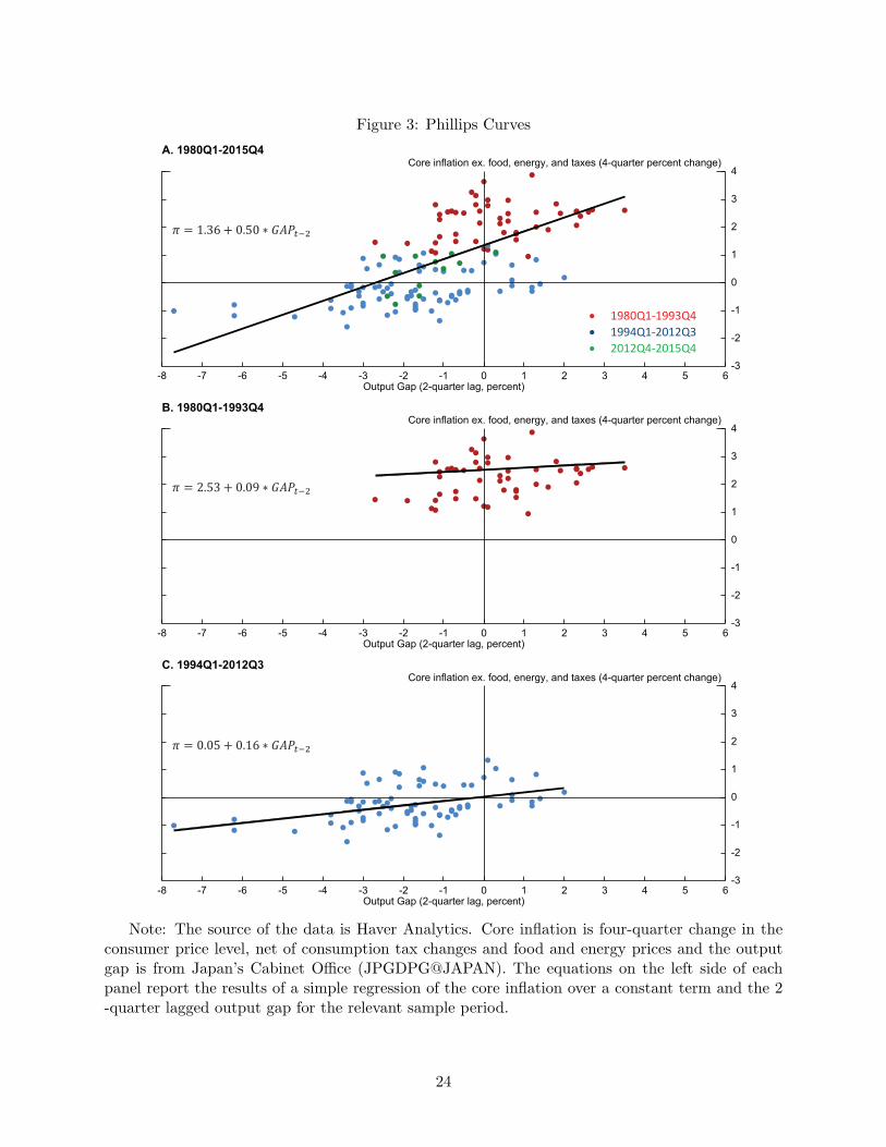
Figure 3: Phillips Curves
-3
-2
-1
0
1
2
3
4
-8 -7 -6 -5 -4 -3 -2 -1 0 1 2 3 4 5 6
A. 1980Q1-2015Q4
Core inflation ex. food, energy, and taxes (4-quarter percent change)
Output Gap (2-quarter lag, percent)
-3
-2
-1
0
1
2
3
4
-8 -7 -6 -5 -4 -3 -2 -1 0 1 2 3 4 5 6
C. 1994Q1-2012Q3
Core inflation ex. food, energy, and taxes (4-quarter percent change)
Output Gap (2-quarter lag, percent)
-3
-2
-1
0
1
2
3
4
-8 -7 -6 -5 -4 -3 -2 -1 0 1 2 3 4 5 6
B. 1980Q1-1993Q4
Core inflation ex. food, energy, and taxes (4-quarter percent change)
Output Gap (2-quarter lag, percent)
· 1980Q1-1993Q4
· 1994Q1-2012Q3
· 2012Q4-2015Q4
Note: The source of the data is Haver Analytics. Core inflation is four-quarter change in theconsumer price level, net of consumption tax changes and food and energy prices and the outputgap is from Japan’s Cabinet Office (JPGDPG@JAPAN). The equations on the left side of eachpanel report the results of a simple regression of the core inflation over a constant term and the 2-quarter lagged output gap for the relevant sample period.
24

Figure 4: Yen, Export Prices, and Import Prices
60
70
80
90
100
110
120
130
140
2007 2009 2011 2013 2015
2012Q3 = 100
Export prices
Import prices
Nominal effectiveexchange rate
Note: The source of the data is Haver Analytics. The nominal effective exchange rate isthe Bank of International Settlement’s Trade Weighted Nominal Effective Foreign Exchange Rate(EERBN@JAPAN). The yen export price series is EPYA10@JAPAN and the yen import priceseries is IPYA10@JAPAN.
25

Figure 5: Japanese Inflation Expectations
-0.5
0.0
0.5
1.0
1.5
2.0
2010 2011 2012 2013 2014 2015
Percent
5y5y forward inflation swap rate
6- to 10-year-aheadConsensus forecast
Note: The sources of the data are Bloomberg and Consensus Economics. The Bloomberg’sticker for the inflation swap rate is FWISJY55 Curncy.
26
Figure 6: Ten-Year Rate
0.0
0.2
0.4
0.6
0.8
1.0
1.2
1.4
2010 2012 2014 2016 2018
Percent
Japanese government bond yield
Forward rate
Note: The source of the data is Bloomberg. The Bloomberg ticker for the 10-year benchmarkJapanese government bond yield is GJGBBNCH Index. The Japanese 10-year forward rate isestimated by the Federal Reserve Board staff based on based on a zero-coupon yield curve model.
27

Figure 7: Inflation Target Shocks: VAR Evidence for Japan in Two Sample Periods
0 10 20 30−1
0
1
2
3Core Inflation, yoy, ppt
0 10 20 30−1
0
1
2
3Long Term Interest Rate, ppt
0 10 20 30−10
0
10
20Real Exchange Rate, %
Quarters0 10 20 30
−2
−1
0
1GDP, %
Quarters
0 10 20 30−1
0
1
2
3Core Inflation, yoy, ppt
0 10 20 30−1
0
1
2
3Long Term Interest Rate, ppt
0 10 20 30−40
−20
0
20Real Exchange Rate, %
Quarters0 10 20 30
−2
0
2
4
6GDP, %
Quarters
Note: The top four panels plot the impulse responses (together with one s.e. bands) to a2 percentage point inflation target shock (3 standard deviations) in the early sample (1974Q1-1993Q4). The bottom four panels plot the impulse responses to a 2 percentage point inflationtarget shock (6 standard deviations) in the late sample (1994Q1-2015Q2).
28

Figure 8: The Contribution of the Identified Inflation Target Shock to
2010 2011 2012 2013 2014 2015 2016
−30
−20
−10
0
10
Start of Abenomics
% d
evia
tion
from
mea
n
Real Exchange Rate Index
ActualContribution of Inflation Target Shocks
2010 2011 2012 2013 2014 2015 2016−2
−1
0
1
2
Start of Abenomics
Core InflationY
OY
, lev
el
Note: The panels are based on a historical decomposition of core inflation and the real exchange rate into the shocks identified by the VAR over 1994Q1-2015Q2.
29

Figure 9: NK Model. Change in Inflation Target under Perfect Credibility
2012 2014 2016 2018
0
0.5
1
1.5%
from
bas
elin
e
GDP
Perfect credibility
Perfect credibility, no ZLB
2012 2014 2016 2018
0
1
2
Perceived Inflation Target
ppt f
rom
bas
elin
e, A
R
2012 2014 2016 2018
0
1
2
Total Inflation
ppt f
rom
bas
elin
e, q
oq, A
R
2012 2014 2016 2018
0
1
2
10−year Expected Inflation
ppt f
rom
bas
elin
e, A
R
2012 2014 2016 2018
0
1
2
Policy Rate
ppt f
rom
bas
elin
e, A
R
Note: The lines plot the impulse response to a 2 percentage point inflation target shock underperfect credibility. The shock takes place over three periods (2012Q4-2013Q2). The solid lines plotthe responses against a baseline where the policy rate is expected to be at zero until 2016Q4. Thedashed lines plot the responses when the policy rate is not constrained by the zero lower bound(ZLB). The first vertical green line identifies the start of Abenomics (2012Q4) and the second onecorresponds to 2015Q2.
30

Figure 10: NK Model. Change in Inflation Target under Imperfect Credibility
2012 2014 2016 2018
0
0.5
1
1.5%
from
bas
elin
e
GDP
Imperfect credibility
Imperfect credibility, no ZLB
2012 2014 2016 2018
0
1
2
Perceived Inflation Target
ppt f
rom
bas
elin
e, A
R
2012 2014 2016 2018
0
1
2
Total Inflation
ppt f
rom
bas
elin
e, q
oq, A
R
2012 2014 2016 2018
0
1
2
10−year Expected Inflation
ppt f
rom
bas
elin
e, A
R
2012 2014 2016 2018
0
1
2
Policy Rate
ppt f
rom
bas
elin
e, A
R
Note: The lines plot the impulse response to a 2 percentage point inflation target shock whenthe inflation target is imperfectly observed. The shock takes place over three periods (2012Q4-2013Q2) against a baseline where the policy rate is expected to be at zero until 2016Q4. The solidlines plot the case when where the policy rate is expected to be at zero until 2016Q4. The dashedlines plot the responses when the policy rate is not constrained by the zero lower bound (ZLB). Thefirst vertical green line identifies the start of Abenomics (2012Q4) and the second one correspondsto 2015Q2.
31

Figure 11: Monte Carlo Experiment
0 10 20 30 40
0
0.5
1
1.5
2
2.5
3Core Inflation, yoy, ppt (ZLB Model)
Quarters0 10 20 30 40
−0.2
0
0.2
0.4
0.6
0.8
1
GDP, % (ZLB Model)
Quarters
DSGE ModelVAR on artificial data, identified with LR restrictionVAR on artificial data, sample size of actual data
0 10 20 30 40
0
0.5
1
1.5
2
2.5
3Core Inflation, yoy, ppt (No ZLB Model)
0 10 20 30 40
−0.2
0
0.2
0.4
0.6
0.8
1
GDP, % (No ZLB Model)
DSGE ModelVAR on artificial data, identified with LR restrictionVAR on artificial data, sample size of actual data
Note: Comparison of impulse responses to a 2 percentage point increase in the inflation target,DSGE model vs VAR on artificial data generated by the DSGE model. Top panels: no ZLB.Bottom panels: ZLB. In each panel, the thick solid lines are the impulse responses from the DSGEmodel with imperfect credibility; the thin solid lines are the mean impulse responses from the VARon artificial data of sample size 1,000, alongside one-standard deviation asymptotic confidenceintervals (dashed lines); the circled lines show the median response calculated averaging 1,000bootstrap replications from sample sizes of length equal to 100.
32
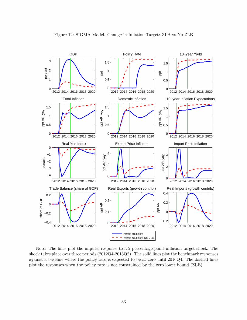
Figure 12: SIGMA Model. Change in Inflation Target: ZLB vs No ZLB
2012 2014 2016 2018 20200
1
2
3
perc
ent
GDP
Perfect credibility
Perfect credibility, NO ZLB
2012 2014 2016 2018 20200
0.5
1
1.5
Policy Rate
ppt
2012 2014 2016 2018 20200
0.5
1
1.5
10−year Yield
ppt
2012 2014 2016 2018 20200
0.5
1
1.5
Total Inflation
ppt A
R, y
oy
2012 2014 2016 2018 20200
0.5
1
1.5
Domestic Inflationpp
t AR
, yoy
2012 2014 2016 2018 20200
0.5
1
1.5
10−year Inflation Expectations
ppt A
R, y
oy
2012 2014 2016 2018 2020
−4
−3
−2
−1
0Real Yen Index
perc
ent
2012 2014 2016 2018 2020
0
2
4
Export Price Inflation
ppt A
R, y
oy
2012 2014 2016 2018 20200
2
4
Import Price Inflation
ppt A
R, y
oy
2012 2014 2016 2018 2020−0.4
−0.2
0
0.2
Trade Balance (share of GDP)
shar
e of
GD
P
2012 2014 2016 2018 20200
0.1
0.2
Real Exports (growth contrib.)
ppt A
R
2012 2014 2016 2018 2020
−0.2
0
0.2
0.4
Real Imports (growth contrib.)
ppt A
R
Note: The lines plot the impulse response to a 2 percentage point inflation target shock. Theshock takes place over three periods (2012Q4-2013Q2). The solid lines plot the benchmark responsesagainst a baseline where the policy rate is expected to be at zero until 2016Q4. The dashed linesplot the responses when the policy rate is not constrained by the zero lower bound (ZLB).
33
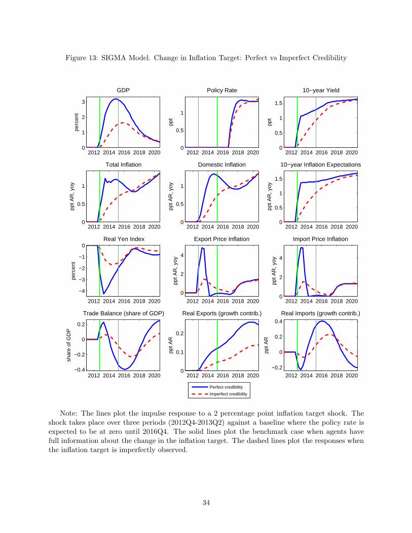
Figure 13: SIGMA Model. Change in Inflation Target: Perfect vs Imperfect Credibility
2012 2014 2016 2018 20200
1
2
3
perc
ent
GDP
Perfect credibility
Imperfect credibility
2012 2014 2016 2018 20200
0.5
1
Policy Rate
ppt
2012 2014 2016 2018 20200
0.5
1
1.5
10−year Yield
ppt
2012 2014 2016 2018 20200
0.5
1
Total Inflation
ppt A
R, y
oy
2012 2014 2016 2018 20200
0.5
1
Domestic Inflationpp
t AR
, yoy
2012 2014 2016 2018 20200
0.5
1
1.5
10−year Inflation Expectations
ppt A
R, y
oy
2012 2014 2016 2018 2020
−4
−3
−2
−1
0Real Yen Index
perc
ent
2012 2014 2016 2018 2020
0
2
4
Export Price Inflation
ppt A
R, y
oy
2012 2014 2016 2018 20200
2
4
Import Price Inflation
ppt A
R, y
oy
2012 2014 2016 2018 2020−0.4
−0.2
0
0.2
Trade Balance (share of GDP)
shar
e of
GD
P
2012 2014 2016 2018 20200
0.1
0.2
Real Exports (growth contrib.)
ppt A
R
2012 2014 2016 2018 2020
−0.2
0
0.2
0.4
Real Imports (growth contrib.)
ppt A
R
Note: The lines plot the impulse response to a 2 percentage point inflation target shock. Theshock takes place over three periods (2012Q4-2013Q2) against a baseline where the policy rate isexpected to be at zero until 2016Q4. The solid lines plot the benchmark case when agents havefull information about the change in the inflation target. The dashed lines plot the responses whenthe inflation target is imperfectly observed.
34

Figure 14: SIGMA Model. Change in the Inflation Target and Exchange Rate Shock
2012 2014 2016 2018 20200
1
2
3
4
perc
ent
GDP
Perfect credibility
Imperfect credibility
2012 2014 2016 2018 20200
0.5
1
1.5
Policy Rate
ppt
2012 2014 2016 2018 20200
0.5
1
1.5
10−year Yield
ppt
2012 2014 2016 2018 20200
0.5
1
1.5
2Total Inflation
ppt A
R, y
oy
2012 2014 2016 2018 20200
0.5
1
1.5
Domestic Inflation
ppt A
R, y
oy
2012 2014 2016 2018 20200
0.5
1
1.5
10−year Inflation Expectations
ppt A
R, y
oy
2012 2014 2016 2018 2020
−8
−6
−4
−2
0Real Yen Index
perc
ent
2012 2014 2016 2018 2020−2
024
68
Export Price Inflation
ppt A
R, y
oy
2012 2014 2016 2018 2020
0
5
10
Import Price Inflation
ppt A
R, y
oy
2012 2014 2016 2018 20200
0.2
0.4
0.6
Trade Balance (share of GDP)
shar
e of
GD
P
2012 2014 2016 2018 20200
0.2
0.4
Real Exports (growth contrib.)
ppt A
R
2012 2014 2016 2018 2020−0.8
−0.6
−0.4
−0.2
0
Real Imports (growth contrib.)
ppt A
R
Note: The lines plot the impulse response to a 2 percentage point inflation target shock coupledwith a risk premium shock that leads to a 15 percent depreciation of the real yen index. Theshock takes place over three periods (2012Q4-2013Q2) against a baseline where the policy rate isexpected to be at zero until 2016Q4. The solid lines plot the benchmark case when agents havefull information about the change in the inflation target. The dashed lines plot the responses whenthe inflation target is imperfectly observed.
35

References
Adolfson, M., S. Laseen, J. Linde, and M. Villani (2007). Bayesian Estimation of an Open Econ-
omy DSGE Model with Incomplete Pass-Through. Journal of International Economics 72 (2),
481–511. [18]
Aruoba, S. B., P. Cuba-Borda, and F. Schorfheide (2016). Macroeconomic Dynamics Near the
ZLB: A Tale of Two Countries. Mimeo. [14]
Ascari, G. and T. Ropele (2012). Disinflation in a DSGE perspective: Sacrifice ratio or welfare
gain ratio? Journal of Economic Dynamics and Control 36 (2), 169–182. [12]
Benigno, G. and L. Fornaro (2015). Stagnation Traps. Working Papers 832, Barcelona Graduate
School of Economics. [21]
Bernanke, B. S., V. R. Reinhart, and B. P. Sack (2004). Monetary Policy Alternatives at the Zero
Bound: An Empirical Assessment. Brookings Papers on Economic Activity 35 (2), 1–100. [2]
Blanchard, O. J., G. Dell’Ariccia, and P. Mauro (2010). Rethinking Macroeconomic Policy.
Journal of Money, Credit and Banking 42 (s1), 199–215. [20]
Blanchard, O. J. and D. Quah (1989). The Dynamic Effects of Aggregate Demand and Supply
Disturbances. American Economic Review 79 (4), 655–73. [3]
Christiano, L., M. Eichenbaum, and S. Rebelo (2011). When Is the Government Spending Mul-
tiplier Large? Journal of Political Economy 119 (1), 78 – 121. [15]
Christiano, L. J., M. Eichenbaum, and C. L. Evans (2005). Nominal rigidities and the dynamic
effects of a shock to monetary policy. Journal of Political Economy 113 (1), 1–45. [9]
Coenen, G. and V. W. Wieland (2004). Exchange-Rate Policy and the Zero Bound on Nominal
Interest Rates. American Economic Review 94 (2), 80–84. [19]
Coibion, O., Y. Gorodnichenko, and J. Wieland (2012). The Optimal Inflation Rate in New
Keynesian Models: Should Central Banks Raise Their Inflation Targets in Light of the Zero
Lower Bound? Review of Economic Studies 79 (4), 1371–1406. [20]
Collard, F., P. Fve, and J. Matheron (2007). The Dynamic Effects of Disinflation Policies. IDEI
Working Papers 426, Institut d’conomie Industrielle (IDEI), Toulouse. [12]
Eggertsson, G., A. Ferrero, and A. Raffo (2014). Can structural reforms help Europe? Journal
of Monetary Economics 61 (C), 2–22. [21]
36

Eichengreen, B. (2013). Japan Rising? The Milken Institute Review , 15–25. [2, 40]
Erceg, C. J., L. Guerrieri, and C. Gust (2006). SIGMA: A New Open Economy Model for Policy
Analysis. International Journal of Central Banking 2 (1). [17, 18]
Erceg, C. J. and A. T. Levin (2003). Imperfect credibility and inflation persistence. Journal of
Monetary Economics 50 (4), 915–944. [4, 11, 12, 13, 20]
Faust, J. and E. M. Leeper (1997). When Do Long-Run Identifying Restrictions Give Reliable
Results? Journal of Business & Economic Statistics 15 (3), 345–53. [15]
Goodfriend, M. and R. G. King (2005). The incredible Volcker disinflation. Journal of Monetary
Economics 52 (5), 981–1015. [4]
Guerrieri, L. and M. Iacoviello (2015). Occbin: A toolkit for solving dynamic models with occa-
sionally binding constraints. Journal of Monetary Economics (70), 22–38. [12]
Hausman, J. K. and J. F. Wieland (2015). Overcoming the Lost Decades? Abenomics after
Three Years. Brookings Papers on Economic Activity . [3, 13]
Ireland, P. N. (2007). Changes in the federal reserve’s inflation target: Causes and consequences.
Journal of Money, Credit and Banking 39 (8), 1851–1882. [4, 12, 14]
Ito, T. (2013). Abenomics: Early Success and Prospects. Japan Spotlight , 1–4. [2]
Ito, T. and F. S. Mishkin (2006). Two Decades of Japanese Monetary Policy and the Deflation
Problem. In T. Ito and A. K. Rose (Eds.), Monetary Policy with Very Low Inflation in the
Pacific Rim, Volume 15, pp. 131–202. The University of Chicago. [2]
King, R. G., C. I. Plosser, J. H. Stock, and M. W. Watson (1991). Stochastic Trends and
Economic Fluctuations. American Economic Review 81 (4), 819–40. [3, 4, 6]
Kollmann, R. (2001). The exchange rate in a dynamic-optimizing business cycle model with
nominal rigidities: a quantitative investigation. Journal of International Economics 55 (2),
243–262. [18]
Krugman, P. R. (1998). It’s Baaack: Japan’s Slump and the Return of the Liquidity Trap.
Brookings Papers on Economic Activity 29 (2), 137–206. [2]
Krugman, P. R. (2014). Timid Analysis. The New York Times, The Conscience of a Liberal,
March, 21. [20]
37

Kuroda, H. (2013). Overcoming Deflation and After. Speech at the Meeting of Councillors of
Nippon Keidanren(Japan Business Federation) in Tokyo by the Governor of the Bank of
Japan. [5, 15]
Mandel, B. R. and G. Barnes (2013). Japanese Inflation Expectations, Revisited. Liberty Street
Economics, Federal Reserve Bank of New York. [5]
Mankiw, N. G. and R. Reis (2002). Sticky Information versus Sticky Prices: A Proposal to
Replace the New Keynesian Phillips Curve. The Quarterly Journal of Economics 117 (4),
1295–1328. [12]
Mertens, K. R. S. M. and M. O. Ravn (2014). Fiscal Policy in an Expectations-Driven Liquidity
Trap. Review of Economic Studies 81 (4), 1637–1667. [14]
Rogers, J. H., C. Scotti, and J. H. Wright (2014). Evaluating Asset-Market Effects of Uncon-
ventional Monetary Policy: A Cross-Country Comparison. International Finance Discussion
Papers 1101, Board of Governors of the Federal Reserve System. [3]
Schaumburg, E. and A. Tambalotti (2007). An investigation of the gains from commitment in
monetary policy. Journal of Monetary Economics 54 (2), 302–324. [21]
Shirai, S. (2013). Monetary Policy and Forward Guidance in Japan. Speeches at the International
Monetary Fund (September 19) and the Board of Governors of the Federal Reserve System
(September 20) Held in Washington, D.C. by Sayuri Shirai, Member of the Policy Board of
the Bank of Japan. [5]
Smets, F. and R. Wouters (2007). Shocks and frictions in us business cycles: A bayesian dsge
approach. American Economic Review 97 (3), 586–606. [9, 10]
Svensson, L. E. (2003). Escaping from a Liquidity Trap and Deflation: The Foolproof Way and
Others. Journal of Economic Perspectives 17 (4), 145–166. [19]
Warne, A. (1993). A Common Trends Model: Identification, Estimation and Inference. Papers
555, Stockholm - International Economic Studies. [3, 6]
38

Appendix
Appendix A Robustness Analysis on the VAR
In Section 3, we showed how Japanese macroeconomic variables respond to an inflation target
shock using a VAR with a long-run restriction identification scheme. The identified increase in the
inflation target leads to a permanent increase in inflation and nominal interest rates, resulting in a
short-lived expansion in economic activity alongside a temporary depreciation of the currency. In
this Appendix, we validate the robustness of our VAR results by applying the same identification
restrictions to a VAR on U.S. data for the period 1970Q1-2015Q2. We estimate the same 5-variable
vector error correction model with core inflation, interest rate, the real exchange rate, and real oil
prices which we formulated and discussed in Section 3.22
Figure A.1 plots the impulse response to the identified inflation target shock for the United
States. When the shock is normalized so that it leads to a 2 percentage point long-run increase in
inflation (corresponding approximately to a 3 standard deviations shock), it leads to a temporary
decrease in real interest rates, to a depreciation of the exchange rate (about 4 percent after one
year), and to a short-run boost in economic activity. In the first year after the shock, GDP is
almost 1.5 percent above the baseline, somewhere in between the response of GDP in Japan for
the two sub-samples.
We also estimated the model excluding the ZLB period, that is truncating the sample at 2007Q4.
We find that the response of output to an inflation target shock is smaller and less front-loaded
than in the pre-ZLB sample. We view this finding as consistent with the hypothesis that inflation
target shocks are more powerful at the ZLB.
Appendix B Risk Premia
Section 4 and 5 showed that the dynamics under imperfect credibility seem to capture reasonably
well the recent Japanese experience. However, they also imply that inflation will rise to 2 percent
very slowly, raising the question of what the BOJ could do to sooner achieve its goal. One way to
break out from this slow adjustment would be to make a much bolder statement about the inflation
target itself. For instance, one possibility would be to temporarily adopt an inflation target higher
than 2 percent, a scenario we explore using the closed-economy model developed in Section 4. In
Figure A.2, we show the responses to an additional boost in the inflation target from 2 to 3 percent
between 2015Q2 and 2016Q4. Following the announcement, the inflation target perceived by the
22 Inflation is the four-quarter change in the consumer price level net of food and energy (S111PCXG@G10). Thereal exchange rate is the JP Morgan Broad Real Effective Exchange Rate Index for the United States, log transformed(Haver mnemonic: N111XJRB@G10). The long-term interest rate is the 10-Year Treasury Note Yield at ConstantMaturity (FCM10@USECON). We extract the business cycle component of real GDP (GDPH@USECON) usinga band-pass filter that selects frequencies between 2 and 32 quarters. Real oil price inflation is calculated as the4-quarter growth rate of WTI (PZTEXP@USECON) minus U.S. CPI 4-quarter inflation
39

agents rise much faster. Accordingly, inflation immediately accelerates and approaches 2 percent
in 2016, much earlier than in the previous case. The resulting lower real rates also provide an
additional lift to GDP.
There may be risks associated with such bolder policies, including the possibility that inflation
might get out of control. Given Japan’s precarious public finances –net debt has risen above 130
percent of GDP according to the OECD– some observers (e.g Eichengreen 2013) have discussed the
possibility that a misstep in the direction of substantially higher inflation might induce investors to
think that fiscal objectives have come to dominate monetary policy, triggering a self-fulling vicious
cycle of destabilizing inflation and debt dynamics. In other words, fears of fiscal dominance or debt
monetization might materialize in case of large enough inflation surprises, prompting a jump in
risk premia. To explore such a scenario, we modify our benchmark new-Keynesian model and allow
for risk premia on government debt which are triggered by increases in the inflation rate above a
certain threshold. More specifically, we re-write the budget constraint, equation (1), as:
ct + kt + ϕt = wtnt + (Rktzt + 1− δ) kt−1 + divt−τ t − bt +Rt−1
πtbt−1 (9)
where the gross interest on government debt Rt−1 = Rt−1 + εt and the risk premium εt follows:
εt =
{α (πt − πt−1) if πt − πt−1 > λ
0 if πt − πt−1 6 λ(10)
where α > 0 is a scaling factor. To the extent that inflation does not accelerate too quickly between
one period and the next, εt = 0, and the model is unchanged. By contrast, when inflation accelerates
quickly, εt is positive and the risk premium shock enters the households’s first order condition for
government debt. Figure A.2 shows the model dynamics when the additional boost to the inflation
target leads to a faster pickup in inflation and, in turn, to a rise in risk premia. We set λ = 0.01
and α = 20, so that when quarterly inflation rises at an annual pace faster than 0.05 percentage
point, risk premia increase roughly 400 basis points after eight quarters, a calibration that mimics
the rise in sovereign risk spreads of the vulnerable euro-area countries during the European debt
crisis. In this scenario, inflation expectations still meet the 2 percent target in 2016, but the rise
in risk premia causes output to fall and the debt-to-GDP ratio to rise 6 percentage points above
baseline. As a result of the dip in output, inflation rises a bit more slowly.
40

Figure A.1: Inflation Target Shocks: VAR Evidence for the United States
0 10 20 30−1
0
1
2
3Core Inflation, yoy, ppt
0 10 20 30−1
0
1
2
3Long Term Interest Rate, ppt
0 10 20 30−6
−4
−2
0
2Real Exchange Rate, %
Quarters0 10 20 30
−1
0
1
2
3GDP, %
Quarters
Note: The panels plot the impulse responses (together with one s.e. bands) to a 2 percentage
point inflation target shock (about 3 standard deviations) in the United States for the period
1970Q1-2013Q4.
41

Figure A.2: NK Model. Change in Inflation Target: Imperfect Credibility and Risk Premia
2012 2014 2016 2018−0.4−0.2
00.20.40.60.8
% fr
om b
asel
ine
GDP
Imperfect credibility
...with additional boost
...with boost and risk premia
2012 2014 2016 2018
0
0.5
1
1.5
2
2.5Perceived Inflation Target
ppt f
rom
bas
elin
e, A
R
2012 2014 2016 2018
0
0.5
1
1.5
2
2.5Total Inflation
ppt f
rom
bas
elin
e, q
oq, A
R
2012 2014 2016 2018
0
0.5
1
1.5
2
2.510−year Expected Inflation
ppt f
rom
bas
elin
e, A
R
2012 2014 2016 2018−1
0
1
2
3
4
5Risk Premium
ppt f
rom
bas
elin
e, A
R
2012 2014 2016 2018
−4
−2
0
2
4
6
Debt to GDP
ppt f
rom
bas
elin
e
Note: The lines plot the impulse response to a 2 percentage point inflation target shock. The
shock takes place over three periods (2012Q4-2013Q2) against a baseline where the policy rate
is expected to be at zero until 2016Q4. The dashed lines plot the responses when the inflation
target is imperfectly observed. The solid lines plot the responses when the target is imperfectly
observed, and the central bank announces a temporary increase in the inflation target from 2 to 3
percent between 2015Q2 and 2016Q4. The dash-dotted lines plot the responses when the target is
imperfectly observed, the central bank announces a temporary increase in the inflation target from
2 to 3 percent between 2015Q2 and 2016Q4, and risk premia reacts endogenously when inflation
increases more than 0.05 percentage point between one quarter and the next.
42


![[Japanese Culture] Japanese Fairy Tale](https://static.fdocuments.us/doc/165x107/577dab5a1a28ab223f8c5222/japanese-culture-japanese-fairy-tale.jpg)