radiosity - Stanford University

CS348B Lecture 17 Pat Hanrahan, Spring 2002

Radiosity

Classic radiosity = finite element method

Assumptions

Diffuse reflectance

Usually polygonal surfaces

Advantages

Soft shadows and indirect lighting

View independent solution

Precompute for a set of light sources

Useful for walkthroughs


Early Radiosity

From Goral, Torrance, Greenberg, Battaile 1984


Early Radiosity

From Cohen, Chen, Wallace and Greenberg 1988


First Radiosity Pictures ...

Parry Moon and Domina Spencer (MIT), Lighting Design, 1948

Finite Element Method


The Radiosity Equation

Assume diffuse reflection only

Solve for radiosity (2D function)

2

( ) ( ) ( ) ( , ) ( )e

M

B x B x x F x x B x dAρ ′ ′ ′= + ∫

2

cos cos( , ) ( , )F x x V x x

x x

θ θπ

′′ ′=

′−

( ) ( ) ( ) ( )eB x B x x E xρ= +

θ ′ x′

dA

x x′−

θ

dA′

x


Classic Radiosity Algorithm

Mesh Surfaces into Elements

Compute Form FactorsBetween Elements

Solve Linear Systemfor Radiosities

Reconstruct and DisplaySolution


Simple Room Scene

Table in room sequence from Cohen and Wallace


Basic Functions

Piecewise constant basis functions

Express radiosity as sum of basis functions

( ) ( )

( ) ( )

( ) ( )

i ii

e i ii

i ii

B x B N x

B x E N x

x N xρ ρ

=

=

=

∑

∑

∑

( )iN x

Constant radiosity assumption


Derivation

Convert integral equation to matrix equation

( , ) ( ) ( )i j

i i i i i j i jj A A

B A E A B F x x N x N x dAdAρ ′ ′ ′= + ∑ ∫ ∫

2

( ) ( ) ( ) ( , ) ( )e j j

M

B x B x x F x x B N x dAρ ′ ′ ′= + ∑∫

( ) ( ) ( ) ( , ) ( )j

i i i i i i j ji i i j A

B N x B N x N x B F x x N x dAρ

′ ′ ′ = +

∑ ∑ ∑ ∑ ∫

( ) ( ) ( ) ( , ) ( )j

i i i i i i j ji i i j A

B N x B N x N x B F x x N x dA dAρ ′ ′ ′ = + ∑ ∑ ∑ ∑∫ ∫


Form Factor

Form Factor

Summation

Form factor is the percentage of light leaving ithat makes it to j

2

cos cos( , )

i j

o ii ij j ji

A A

A F A F V x x dAdAx x

θ θπ

′′ ′= =

′−∫ ∫

1ijj

F =∑


Classic Radiosity

Power balance

Linear system of equations

i i i i i j i ijj

B A E A B AFρ= + ∑

1 11 1 12 1 1 1 1

2 21 2 22 2 21 2 2

1 2

1

1

1

n

n n n n n nn n n

F F F B E

F F F B E

F F F B E

ρ ρ ρρ ρ ρ

ρ ρ ρ

− − − − − − = − − −

i i i ij jj

B E F Bρ= + ∑

Form Factors


Hemicube Algorithm

First radiosity algorithm to deal with occlusion1. Render scene from the point of view of each

vertex/element2. Compute delta form factors – contribution from each

pixel

Typical resolution: 32x32

Render source elements from POV of receiving element

,i j

j

dA A pp A

F F∈

= ∆∑


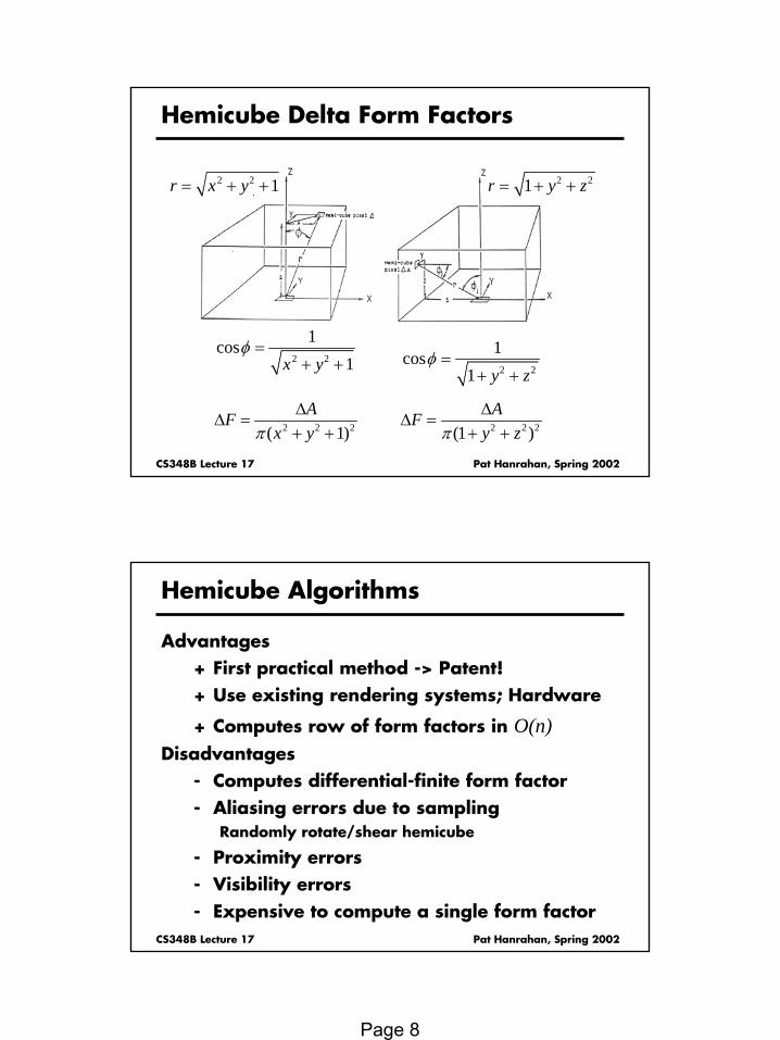
Hemicube Delta Form Factors

2 2 2( 1)

AF

x yπ∆

∆ =+ +

2 2 1r x y= + + 2 21r y z= + +

2 2

1cos

1x yφ =

+ + 2 2

1cos

1 y zφ =

+ +

2 2 2(1 )

AF

y zπ∆

∆ =+ +


Hemicube Algorithms

Advantages+ First practical method -> Patent!+ Use existing rendering systems; Hardware

+ Computes row of form factors in O(n)Disadvantages

- Computes differential-finite form factor- Aliasing errors due to sampling

Randomly rotate/shear hemicube

- Proximity errors- Visibility errors- Expensive to compute a single form factor

Solving


Solve [F][B] = [E]

Direct methods: O(n3)

Gaussian eliminationGoral, Torrance, Greenberg, Battaile, 1984

Iterative methods: O(n2)

Energy conservation → diagonally dominant → iteration converges

Gauss-Seidel, Jacobi: GatheringNishita, Nakamae, 1985Cohen, Greenberg, 1985

Southwell: ShootingCohen, Chen, Wallace, Greenberg, 1988


Gathering

Row of F times B

Calculate one row of F and discard

for(i=0; i<n; i++)B[i] = Be[i];

while( !converged ) {for(i=0; i<n; i++) {E[i] = 0;for(j=0; j<n; j++)E[i] += F[i][j]*B[j];

B[i] = Be[i]+rho[i]*E[i];}

}


Successive Approximation

eL

e eL K L+eL

eK L eK K L eK K K L

2e eL K L+ 3

e eL K L+


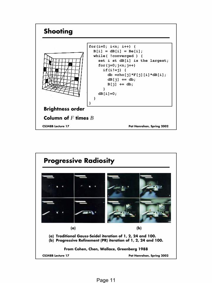
Shooting

Brightness order

Column of F times B

for(i=0; i<n; i++) {B[i] = dB[i] = Be[i];while( !converged ) {set i st dB[i] is the largest;for(j=0;j<n;j++)if(i!=j) {db =rho[j]*F[j][i]*dB[i];dB[j] += db;B[j] += db;

}dB[i]=0;

}}


Progressive Radiosity

(a) Traditional Gauss-Seidel iteration of 1, 2, 24 and 100. (b) Progressive Refinement (PR) iteration of 1, 2, 24 and 100.

(a) (b)

From Cohen, Chen, Wallace, Greenberg 1988

Meshing


Accuracy

Uniform MeshReference Solution

Table in room sequence from Cohen and Wallace


Artifacts

Error ImageA. Blocky shadowsB. Missing featuresC. Mach bandsD. Inappropriate shading discontinuitiesE. Unresolved discontinuities


Increasing Resolution


Adaptive Meshing


Discontinuity Mesh

From Baum et al.


Discontinuity Mesh

From Campbell et al.


Discontinuity Meshing

From Lischinski, Tampieri, Greenberg 1992


Hierarchical Radiosity


Summary

Remember assumptionsDiffuse reflectancePolygons

Difficult to relax assumptionsComputation challenges

MeshingComplex input geometryComplexity due to shadows

Dense couplingO(n2) matrix elements

HR leads to O(n) algorithm (ignoring discontinuities)

radiosity - Stanford University

Documents

Transcript of radiosity - Stanford University