Radiosity: A Study in Photorealistic Renderingby

Christopher De Angelis

Undergraduate HonorsThesis Computer Science Department – Boston College Submitted May 1, 1998

2

Introduction

For thousands of years, man has had a fascination with visually depicting theworld in which he lives. From cave paintings to the startlingly real paintings of the HighRenaissance, there is no question that this hobby has been preserved and continuallyreinterpreted throughout the history of mankind. Now we are at a point where man isexperimenting in depicting not just with the tools of traditional artistry but with the aid ofthe computer, and we are finding some fascinating results.

Between all the methods of computer graphics - which is essentially a marriageof mathematics and computer hardware - one of the most compelling yet perhaps mostoverlooked areas is that of radiosity. I find it compelling because of its amazing abilityto generate images that look nearly true to life. Although you don't hear much aboutradiosity unless you read the technical journals of computer graphics, such as theComputer Graphics publication of the ACM SIGGRAPH group, there has been a fairamount of research and development in the academic circle. This being the case, mypatient advisor, William Ames, encouraged me to start the process of understandingjust what radiosity is and how it works by using the original sources rather than latterreformulations. Although I was often frustrated by the progress of my work, I believethis ended up being a solid approach for understanding the method and thenimplementing a radiosity renderer of my own. This paper serves to summarize myfindings and efforts with a fair amount of detail and to give some insights as to whyradiosity is fascinating but has not generated all that much in the way of widespreaddevelopment efforts.

I. Radiosity: What is it?

1.1: General Description and Usefulness

The first thing to realize about radiosity is that it is not an algorithm for renderinginteractive 3-D graphics like those in modern computer games. The ever-presenttradeoff of accuracy vs. speed still prohibits the use of realistic graphics in games ontoday's hardware - at least in real-time computations. Instead of interactiveapplications, the camp of rendering that radiosity does belong to is that of photo-realism, that is, the quest to generate images on the computer that are very similar tophotographs.

Within the category of photorealistic rendering, the two main approaches are raytracing and radiosity, ray tracing being the more common one. (It is valuable to talkabout ray tracing here since the discussion will provide a frame of reference for thepros and cons of radiosity as a method in the photorealism camp.) Images generatedby ray tracing are often used in entertainment and advertising industries. For example,ray tracing is the algorithm that Pixar employed to generate the highly successfulDisney film "Toy Story" - the world's first feature length film to be generated entirely bya computer graphics rendering algorithm. Outside the commercial realm, freelydistributable versions of ray tracers are readily available to computer graphicsenthusiasts, such as Persistence of Vision (POV-RAY). Ray tracing tends to produceimages that look rather glossy and polished - often nearly too polished. This isbecause ray tracing works by modeling the objeccts of the scene and is especially

3

concerned with scene geometry. More specifically, the nature of ray tracing involvescasting simulated rays of light from a single viewpoint in 3-dimensional space throughevery pixel location on the screen and is dependent on information regarding objectintersections before doing any image rendering. This process results in excellentrepresentations of specular reflections and refraction effects (a specular light comesfrom a particular direction and is reflected sharply towards a particular direction;specular light causes a bright spot on the surface it shines upon, referred to as thespecular highlight. One example would be the shiny spot on a balloon directly in thepath of a light source). However, due to the fact that ray tracing renders scenes basedon the definite location of the observer, it is what is known as a view-dependentalgorithm. The consequence of being a view-dependent algorithm is that in order to beviewed from a different vantage-point, the entire scene must be re-rendered. Inaddition, in order to better simulate the effect of a particular object contributing itsillumination towards all other objects in the scene, a directionless ambient lighting termmust be arbitrarily added into the scene. This consequence makes ray tracing what iscalled a local illumination algorithm, that is, one where the light travels directly from thesource to the surface being illuminated - in other words, direct illumination.

(image 1 - a ray traced image showing specular reflection & refraction - by J. Arvo)

In contrast, the goal of radiosity is not to model the objects of the environment,but rather the lighting of the environment. As we will see in the detailed description, itspends a significant amount of time dealing with issues of scene geometry, but thepurpose of this is to make many minute light calculations which combine to describe theentire scene. The information gathered in this step - referred to as the form factordetermination - is computed entirely independent of surface properties of each entity orpatch in the scene. The result of this form factor computation is a description of theamount of light from a particular patch reaching every other patch in the scene.Because this object-to-object lighting information is a key part of the rendering processhere, radiosity is categorized as a global illumination algorithm; that is, the interaction oflight amongst all objects in the scene is considered for total illumination in the scene,eliminating the need for adding an arbitrary, ambient lighting term. Since the

4

information from the form factor computation is then used in combination with thesurface property data to produce an image of the scene without any other light sourceinformation, the radiosity method generates images that accurately model diffusereflections, color bleeding effects, and realistic shadows (diffuse lighting comes from aparticular direction but is reflected evenly off a surface, so although you observebrighter highlights when the light is pointed directly at a surface rather than hitting thesurface at an angle, the light gets evenly distributed in all directions; fluorescent lightingis a good example of diffuse lighting). It turns out that these are the types of effects weobserve frequently in every day living. In addition, since radiosity models its scenesusing information inherent to the scene geometry and surface properties alone, it is aview-independent algorithm, meaning that that the vantage-point of the observer isirrelevant to the rendering process. The consequence here is that after the costlycomputation of the form factors is completed once, the viewer's vantage-point can bechanged to any location pretty quickly. This presents the possibility of a nearly real-time walkthrough of a scene that has been computed via radiosity. So as in the case ofray-tracing, you cannot produce an animation of objects in the scene withoutrecomputing the entire scene image from scratch, but you can use the advantages ofview-independence to create a pretty fast walkthrough of a static scene using a typicalhome computer of the 1990's.

One industry that is using radiosity to create walkthroughs is that of architecturaland interior design. The radiosity method is proving itself useful in applications ofvirtual tours of buildings designed but not yet built by architectural and interior designfirms; this would be advantageous for a customer who is not quite sure aboutcommitting to a particular job or is having trouble deciding between several options. Anexample of a still done by the architectural firm Hellmuth, Obata and Kassabaum, Inc.,is shown below in figure 3. So in the sense that you can demonstrate what a particulardesigned or imagined environment might look like, radiosity can be used as asimulation tool. Though in the sense that it does not allow you to dynamically changethe scene, it isn't a true tool for simulation. But until computers become powerfulenough to entirely recompute scenes via radiosity in real-time, this is the price of suchaccuracy. Although some video games claim to use radiosity in their graphics engines,what they must really mean is that they use some ideas borrowed from radiosityrendering theory as no interactive game could possibly produce scenes generated byradiosity in real-time with hardware such as it is at the time of this writing. But one daythis too will change.

(image 2 - an image generated by Ian Ashdown's radiosity program "HELIOS", demonstratingdiffuse reflections & color bleeding - notice these effects on the walls and the objects in thecenter of the scene, respectively. This image was also generated using anti-aliasing.)

5

(image 3 - a radiosity-generated image of the New York Hospital modelled by the architecturalfirm Hellmuth, Obata, and Kassabaum, Inc.)

1.2: The Original Radiosity Algorithm

An exhaustive explanation of the code of a radiosity based renderer would notbe helpful without understanding the details of the theory by itself. In fact, a detailed,line-by-line description of a radiosity implementation would be too tedious to read. Myintent, therefore, is to give a summary of the principles behind the method of radiosityand then discuss non-trivial details of my implementation and implementations ingeneral.

Radiosity was first introduced to the computer graphics community by a group ofresearchers at Cornell University in 1984. It is based on principles of radiation heattransfer useful in calculating heat exchanges between surfaces. These principles arebasically concerned with calculating the total rate at which energy leaves a surface (thequantity of radiosity itself) - in terms of energy per unit time and per unit area - basedon the properties of energy emission and reflectivity particular to a surface. To put itmore succinctly, the radiosity of a surface is the sum of the rates at which the surfaceemits energy and reflects or transmits it from that surface or other surfaces. This is aninteresting idea to apply to computer generated images as the human eye sensesintensities of light; the intensity of light can be approximated well by summing the lightemitted plus the light reflected. The observer only perceives a total energy flux and isunable to distinguish between the two components of light energy. But this is not quiteall there is to computing radiosity. In order to calculate the total quantity of lightreflected from a Lambertian (diffuse) surface, the surface reflectance must bemultiplied by the quantity of incident light energy arriving at a surface from the othersurfaces in the environment. Now the quantity of radiosity for a particular patch (j)can be formulated as shown below in figure 1:

(figure 1 - the general formulation of radiosity by Goral, et. al.)

where B denotes the radiosity, E denotes the energy emission, rho (p) denotes thesurface reflectance, and H denotes the incident light energy arriving at a surface fromthe other surfaces in the environment. Since H for a particular patch j is dependent on

jjjj HEB ρ+=

6

the geometry of all other patches in the scene, it must be computed by essentiallysumming the fraction of energy leaving a patch j and arriving at patch i for all suchpatches i in the scene. This quantity of the fraction of energy leaving surface j andarriving at surface i is known as the form factor. But since the form factors are purelydependent on shape, size, position and orientation of the surfaces in the scene (thescene geometry), it is perhaps better to describe a form factor as a quantity describingthe relative amount of energy that can be "seen" between a pair of patches. Naturally,if elements of the scene block the path of energy transfer between patches i and jwithin the scene, there will be no contribution of light energy from patch i onto patch j(note: the original paper by Goral, Terrance, Greenberg and Bataille is written assumingunoccluded environments, but the radiosity method is easily extended, as I have done,for handling complex environments where there is occlusion of patches by otherpatches). Now the radiosity equation can be expressed in its entirety as follows, with Fdenoting the form factor between patches i and j:

(figure 2 - the full radiosity equation - Goral, et. al.)

The B values (radiosities) computed from this equation are essentially the intensities orbrightnesses of each patch to be rendered in the scene. But all you have is abrightness - that is, there is no color information. So in order to display images of colorinstead of varying shades of gray, the radiosity values must be solved with differentemissivity and reflectivity values for each of the three color bands used in computergraphics: red, blue and green. This is actually of little consequence in terms ofcomputing time since the form factors themselves - which demand the vast majority ofcomputing time - are not dependent on the surface properties. Finally, in order to gainthe benefits of this light intensity information that was worked so hard for, interpolated,or, smooth shading must be performed between coplanar patches so that the scenedoesn't just look like a bunch of patches of slightly different, uniform colors.

Before getting into the messy business of computing form factors - again, wherethe bulk of the time in a radiosity implementation is spent - first consider theassumptions that go along the above method. This method assumes that everysurface in the scene is a convex polygon that can be subdivided into a mesh ofelements, or, patches. As we will see later, a surprisingly significant part of a radiosityimplementation is concerned with the meshing of surfaces in the scene so that theradiosity computations can be performed. Perhaps the most important assumption ofall with radiosity in terms of the final result is the fact that all surfaces (and therefore allpatches) are assumed to be ideal diffuse reflectors. Again, this means that they reflectlight equally in all directions regardless of the angle of the incoming light rays. So as tonot miss the forest for the trees, all of this means that radiosity is good for modelinglarge structures in many scenes encountered in everyday experiences, such as floors,ceilings, walls, furniture, etc., but it does not account for any specular reflection orrefraction of light as seen in glass objects like soda bottles.

NjforFBEBN

iiji

jjj ,1__

1

=+= ∑=

ρ

7

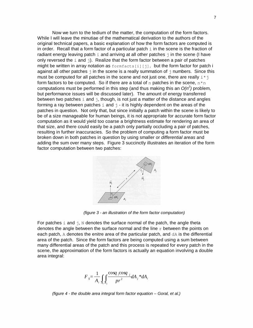
Now we turn to the tedium of the matter, the computation of the form factors.While I will leave the minutiae of the mathematical derivation to the authors of theoriginal technical papers, a basic explanation of how the form factors are computed isin order. Recall that a form factor of a particular patch i in the scene is the fraction ofradiant energy leaving patch i and arriving at all other patches j in the scene (I haveonly reversed the i and j). Realize that the form factor between a pair of patchesmight be written in array notation as formfacts[i][j], but the form factor for patch iagainst all other patches j in the scene is a really summation of j numbers. Since thismust be computed for all patches in the scene and not just one, there are really i*jform factors to be computed. So if there are a total of n patches in the scene, n*ncomputations must be performed in this step (and thus making this an O(n2) problem,but performance issues will be discussed later). The amount of energy transferredbetween two patches i and j, though, is not just a matter of the distance and anglesforming a ray between patches i and j - it is highly dependent on the areas of thepatches in question. Not only that, but since initially a patch within the scene is likely tobe of a size manageable for human beings, it is not appropriate for accurate form factorcomputation as it would yield too coarse a brightness estimate for rendering an area ofthat size, and there could easily be a patch only partially occluding a pair of patches,resulting in further inaccuracies. So the problem of computing a form factor must bebroken down in both patches in question by using smaller or differential areas andadding the sum over many steps. Figure 3 succinctly illustrates an iteration of the formfactor computation between two patches:

(figure 3 - an illustration of the form factor computation)

For patches i and j, N denotes the surface normal of the patch, the angle thetadenotes the angle between the surface normal and the line r between the points oneach patch, A denotes the enitre area of the particular patch, and dA is the differentialarea of the patch. Since the form factors are being computed using a sum betweenmany differential areas of the patch and this process is repeated for every patch in thescene, the approximation of the form factors is actually an equation involving a doublearea integral:

(figure 4 - the double area integral form factor equation – Goral, et al.)

ijA A

ji

iij dAdA

rAF

i j

*coscos1

2∫∫=π

θθ

8

From this equation, it is clear that the angles between the surface normal and the line rare important in the form factor computation. Being the distance between the twodifferential patches, r is easily computed after doing tedious operations on the originalpatch coordinates, but it is not clear how these angles are computed from a first glance.Apparently the authors of the original paper assumed it was trivial to describe how toderive these angles, which I am computing using some vector algebra based on thesurface normal and the vector between the two patches (direction depending on whichpatch is being referred to). Specifically:

surface normal (N) • i-j vector (V)cos theta = -------------------------------------

| length of N | * | length of V | • = dot product * = regular multiplication

A more efficient method of computing form factors than the equation shown in figure 4can be realized without greatly changing the conceptual model of the computation.Although I originally tried using this form of the equation I was unsuccessful and not ina position to debug that implementation very well as I am not familiar with the mathinvolved (see the implementation section for details). The math involved is anapplication of Stokes' theorem to transform the area integrals into contour integrals,which can apparently be computed in less time than the area integrals:

(figure 5 - the contour integral form of the form factor equation – Goral, et.al.)

Finally, there are a few properties of form factors which prove to be useful in theimplementation:

1. There is a reciprocity relationship for radiosity distributions which arediffuse and uniform over each surface:

Ai*Fij = Aj*Fji

This means that knowing Fij also determines Fji, saving significant, butlinear computing time.

2. In a closed environment of n surfaces, there will be total conservation ofenergy, so all of the energy leaving a surface must be accounted for.One can check whether or not the implementation of a closed scenesums nearly to unity as it would if the computer didn't have to approximate the integral:

3. For a convex surface (one that does not see itself):

∫ ∫ ++=i jC C jijiji

iij dzdzrdydyrdxdxr

AF ])ln()ln()[ln(

21π

∑=

==N

jij NiforF

1

,1___1

9

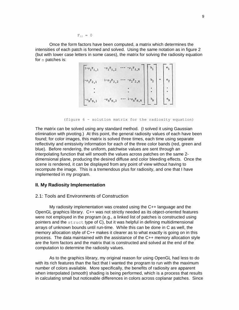
Fii = 0

Once the form factors have been computed, a matrix which determines theintensities of each patch is formed and solved. Using the same notation as in figure 2(but with lower case letters in some cases), the matrix for solving the radiosity equationfor n patches is:

(figure 6 – solution matrix for the radiosity equation)

The matrix can be solved using any standard method. (I solved it using Gaussianelimination with pivoting.) At this point, the general radiosity values of each have beenfound; for color images, this matrix is solved three times, each time using separatereflectivity and emissivity information for each of the three color bands (red, green andblue). Before rendering, the uniform, patchwise values are sent through aninterpolating function that will smooth the values across patches on the same 2-dimensional plane, producing the desired diffuse and color bleeding effects. Once thescene is rendered, it can be displayed from any point of view without having torecompute the image. This is a tremendous plus for radiosity, and one that I haveimplemented in my program.

II. My Radiosity Implementation

2.1: Tools and Environments of Construction

My radiosity implementation was created using the C++ language and theOpenGL graphics library. C++ was not strictly needed as its object-oriented featureswere not employed in the program (e.g., a linked list of patches is constructed usingpointers and the struct type of C), but it was helpful in defining multidimensionalarrays of unknown bounds until run-time. While this can be done in C as well, thememory allocation style of C++ makes it clearer as to what exactly is going on in thisprocess. The data maintained with the assistance of the C++ memory allocation styleare the form factors and the matrix that is constructed and solved at the end of thecomputation to determine the radiosity values.

As to the graphics library, my original reason for using OpenGL had less to dowith its rich features than the fact that I wanted the program to run with the maximumnumber of colors available. More specifically, the benefits of radiosity are apparentwhen interpolated (smooth) shading is being performed, which is a process that resultsin calculating small but noticeable differences in colors across coplanar patches. Since

10

I wanted to be able to fully see the fruits of this labor, I realized long ago that I wouldneed the ability to display the rendered scene in a color depth of 24 bits per pixel (bpp),that is, the palette would have to contain a total of 16,777,216 color entries. This is themaximum number available on most displays and probably many more than the humaneye is capable of distinguishing between. This being the case, I thought about whatplatform it would be practical to develop the program on, along with which graphicslibrary to use. Here at Boston College, I was unsure of the capabilities of the videohardware in the Digital Alpha machines available to Computer Science majors, so Ididn't consider the Alphas as a viable option. As much as I didn't want to buy anything Ididn't already have, I figured that using my own machine with Linux might not work toowell because I can never manage to get X Windows to display in 24 bpp color depth.So I decided I would be best off working in an environment where I was sure of what Icould get in terms of video power, which meant using a Microsoft Windows operatingsystem for the platform. I wound up using the Microsoft Visual C++ 5.0 developmenttools, which come with the libraries and header files for OpenGL (I ran this on WindowsNT Workstation 4.0). Although I was at first hesitant to develop under Windowsknowing that it takes about 100 lines of straight C code to produce a Window that says"Hello World", my task was made much easier thanks to the Auxiliary (AUX) library thatcomes with the Microsoft implementation of OpenGL. The AUX library, among otherthings, took care of all the tedium of making calls to the operating system to open awindow - this may not sound like much, but under Windows it is. It also came in handyfor doing keyboard input; the OpenGL specification makes no provision for input since itstrives to be a platform independent library (the use of keyboard input will be discussedin section 2.6, "Walkthrough Ability"). These and other functions performed by AUXLiband the OpenGL calls allowed me to concentrate on the problem of radiosity itselfrather than having to worry about the details of graphics programming under theoperating system being used. And since OpenGL is so widely available, this programshould run under any operating system with an ANSI C++ compiler and an OpenGL orcompatible library. The Digital UNIX server owned by the Computer Sciencedepartment at Boston College now has Mesa - an OpenGL compatible library -available for general use. Although the X Windows display, in most cases, does notshow all the colors being used by the program and dithering gets performed, it is nice tosee that simply by changing a couple of the header files, the program compiles andruns without a hitch.

The source code is about 1800 lines, or 50 kilobytes, and the executable filesize on both Windows and UNIX machines is roughly 170 kilobytes. The only librarieslinked besides the OpenGL libraries are stdio, stdlib, and math.

2.2: General Program Flow

The program must first read in all patch information from a scene file (seeAppendix A for a description of the scene file) and construct a linked list of patches.The initialize routine performs file parsing, construction of a linked list of patches,subdivision of patches into smaller pieces (discussed in section 2.4, "Area Based PatchSubdivison") and allocation of arrays for storing the form factors, solution matrix, andradiosity values. Patch areas are also calculated by the initialization routine to reduceeffort needed to prepare the scene file. Upon completing the initialize routine, thelengthy routine of computing the form factors is called (aspects of which are discussed

11

in section 2.3, "Form Factor Computation"). Once this lengthy computation is complete,the matrix is prepared and solved three times for the three color values for each patch,the radiosities are normalized so that all values are fractions of the largest radiosityvalue, and radiosity values are assigned to each patch structure and at the vertices(discussed in section 2.5, "Computation of Radiosity Values at Vertices for SmoothShading"). This may sound like an awful lot of work, but it is actually much lessdemanding than the form factor computation.

None of the above is performed by OpenGL. OpenGL does, however, play animportant role in this program by handling the tasks of performing the perspectiveprojection transformations so as to get a better sense of depth, the viewpoint definition,and performing smooth shading on the patches to be rendered once the vertexradiosities have been computed. The automation of the smooth shading calculation inparticular saves a significant effort in doing this manually. I consider myself fortunate tohave done this project at a time when these "low-level" foundations of computergraphics are provided for in the graphics library, allowing more attention to be paid tothe rendering algorithm itself.

2.3: Form Factor Computation

The first method of form factor computation I tried was the contour integral formas cited by Goral, et. al. My understanding is that this form of the equation is moreefficient as the contour integral is an "edge integral" and can be computed withouthaving to step through differential areas as with the area integral. But not beingfamiliar with contour integrals beforehand, I didn't really know what I was doing. Evenafter getting some notion of how this equation should work from Professor HowardStraubing and reviewing the pseudocode of the computation in the original radiositypaper, I was still unable to get the computation to run successfully. The computationinvolves natural logarithms, and I was getting negative numbers from these logs whenr < 1 (see figure 5). This shouldn't have happened. After spending much effort tryingto see what was going wrong using the DBX debugger on UNIX (which seemedappropriate since these were simply calculations for which I needed no graphicaloutput), I finally gave up and decided to use the originally derived, double area integralform of the equation. Things went a lot better once I started using this equation; I got itworking within a few weeks instead of spending two months debugging this phaseunfruitfully. This area integral form is less efficient, but just as accurate as the contourintegral form. Moreover, there is a problem using the contour integral form for whichthere is no obvious solution. When using this form of the equation, one must evaluateln(r), where r is the distance between points on two patches, but when r goes tozero, there is some question as to how to deal with negative infinity. The paper byGoral, et. al. states that this occurs when two patches being used in the computationshare an edge, and the integral was evaluated analytically in this case to both avoidthis problem and imporve the accuracy of the integration. An analytical solution to theintegral would take an additional amount of time to develop, and since I am not familiarwith contour integral math to begin with, I would have to have someone else developthis solution completely independently.

No matter which of these two forms is used to compute the form factors, though,there is an important element to realize here. Both equations are double integrals, and

12

ordinarily they are solved iteratively rather than analytically. Solving them iterativelywith the computer means that some kind of approximation will be done instead ofgetting a definitively accurate answer. So the bottom line is that the accuracy of theform factor computation depends on how finely divided the steps are betweendifferential areas on each patch. The larger the distance between differential areas,the more coarse an estimate of energy coupling between two patches results.Likewise, the smaller the distance, the more accurate the resulting estimate. Naturally,there is a great difference in speed here as well, illustrating one of many recurringinstances of the efficiency-accuracy tradeoff in problems of engineering and computerscience. Statistics demonstrating this principle will be given in section 2.8,"Performance Issues".

The original paper by Goral, et. al. assumes that the scene being modelled hasno occluded surfaces. Subsequent papers and books on radiosity say that not onlydoes the original formulation not account for occluded surfaces but that the contourintegral formulation cannot be extended for occlusion. However, I have been able toincorporate a routine into my implementation of the form factors computed by areaintegrals that checks for occluded surfaces and works with a fair degree of success.The routine I have included in my program adds a factor of N to the complexity to therun-time behavior and is based on ray tracing techniques for testing whether or not theline between the two points on each of the differential patches intersects with any othersurface in the scene. But this tests only whether or not the line intersects with theinfinite plane - not the actual patch. So if there is an intersection found with the infiniteplane based on a particular patch's geometry, a test is then done to see the lineactually intersects with the finite patch in question. For an arbitrary polygon, this isdifficult to do - at least not without a knowledge of what the geometry of the patch isand branching to the appropriate code fragment for that polygon. In my case, though,since I am assuming only convex quadrilaterals and have actually developed scenesusing only quadrilaterals that are rectangles, the intersection test is not very difficult.Actually, for non-quadrilaterals, an infinite plane intersection wouldn't do at all, but itcan save some time for scenes with many quadrilateral patches. But there is animportant subtelty here. In using the double area integral version of the form factorequation, an occluding patch is not truly occluding. It can act as translucent rather thanopaque because light received by one side of the flat quadrilateral can be partiallyabsorbed and partially reflected back into the environment on its other side! So inorder to have a truly occluding patch between a pair of patches in my program, twopatches must be stacked adjacent to each other and separated only by a small amountrelative to the dimensions of the scene.

2.4: Area Based Patch Subdivision

An important piece of information for the routine that computes the form factorsis the area of a particular patch. Originally, I was computing the areas of the patches inmy scene while sketching the scene with vertices labelled on paper and encoding theminto the scene file for input. But I realized that this was entirely too tedious if I wantedto try preparing more complex scenes or modifying existing scenes. The user shouldnot have to do this calculation and put it into the scene file. So I had the program breakthe convex quadrilaterals into two triangles, compute the area of each triangle, andthen add the two areas to determine a single patch area. This is a nice feature to have,

13

and I suspect most other radiosity implementations do some form of patch areacalculation, provided the program is able to determine enough information about thegeometry of the patch (if more than one patch geometry is being handled - not in mycase though). But it still meant that every patch in the scene had to be calculated byhand. This is not such a great thing if one wants to be able to define more complexscenes without a lot of hassle. In addition, the benefits of radiosity can't be trulyappreciated unless the patch size is sufficiently small because a few large patcheswould result in coarse images.

I solved this problem of having to define each and every patch manually byextending the usefulness of the patch area calculation. Since I had this funcitonworking, I decided to use it to figure out the size of a particular patch after it has beencompletely inputted and compared it to a threshold for the maximum allowable patcharea. If the patch is less than or equal to this area, it remains in the linked list and theprogram continues creating the linked list of patches. However, if the patch area islarger than the threshold, the program figures out how many pieces the patch needs tobe broken into, and that number of patches is created automatically using the vertexinformation from the patch read in. These patches are inserted into the linked list andthe patch that was read in originally is deleted after this process is complete. This isanother feature that makes a radiosity renderer a lot more useable by someone whowants to use it with a minimum amount of effort. It turns out that this is not just anenhancement that most programs implement, but that a lot of research in radiosityactually goes into the issue of patch subdivision. The problem of patch subdivision, ormeshing, represents a significant part of the research done in radiosity techniques,even though it does not directly affect the radiosity equation itself. But its importancecomes into play in trying to produce truly photorealistic images since it is desireable tohave both small patches for accuracy and to reduce scene preparation effortsimultaneously.

2.5: Computation of Radiosity Values at Vertices for Smooth Shading

Once the matrix for computing radiosity values has been solved (see figure 6),the patchwise radiosity values are obtained and the scene can be rendered. But ifeach quadrilateral patch is simply drawn with a different color, you wind up with just that- a scene that looks like a bunch of differently colored quadrilaterals. Despite thedifferences that may be observed across a number of patches looked at together, theeffects of diffuse reflections, color bleeding, and shadows cannot be observed. This isbecause simply drawing the patches of different radiosities is done with "flat" shading,where a patch has a uniform color. What really needs to be done in order to see thebenefits of the radiosity computation is rendering the patches using interpolated or"smooth" shading. In order to do this, the routine that performs the smooth shadingmust know the colors of each vertex of the polygon to be shaded and drawn. But thecomputation as originally described only produces radiosity values for patches, not forthe vertices of each patch. So the problem of producing a photorealistic image withradiosity becomes a matter of being able to find the radiosity values of each vertex of apatch.

Of significant importance in solving this problem as I have done is an additionalstep in the portion of the initialization routine that subdivides a patch into smaller pieces

14

according to the maximum area threshold. With each patch node, there are fourpointers for a patch's immediate neighbors sharing edges, i.e., a pointer to a patchlocated to the left, right, upward or downward of the patch in question. After a largepatch has been completely subdivided into its smaller pieces, a second pass through allthe subpatches is performed to determine whether or not a particular patch has theseneighbors, and if it does, the pointer is assigned to the appropriate patch. If a patchdoes not need to be subdivided, then the pointers are simply set to null as the smoothshading is dependent on computing color values at the vertices using coplanar patchesonly. That is, if a patch is not broken down into smaller patches, it will not be coplanarwith any other patch in the way I have designed my program and scene file format, sothere is no need to set pointers to neighboring patches.

Much later in the program, after radiosity values for the patches have beencomputed and those values are explicitly assigned to the patches, a routine is called todetermine set the radiosity values at the vertices of the quadrilateral patches. Thisroutine must loop through all patches in the scene and do lookups for the patch colorsof the three adjacent patches at all four vertices and for each of the three color bands(red, green and blue). This means there are 36 lookups done for each patch. For eachpatch vertex, the radiosity value for each neighboring patch is taken into account for aweighted average of the patch colors to find the specific "vertex radiosity"; again, thisprocess is repeated three times at each vertex to get all required color information. Ifthe neighboring patch in a particular direction does not exist, it is not taken account intothe weighted average. All of this sounds like a lot of work, but it is not all thatsignificant in terms of the overall run-time of the program. Once this is completed,OpenGL can render a series of smooth shaded quadrilaterals making up the sceneafter being told the colors and coordinates of the four patch vertices. Programming thisrequired a lot of thought and effort once the radiosities were being computed correctly,but it was well worth it to see the images the program started producing. See AppendixB for color plates of flat and smooth shaded images of the same scene.

2.6: Walkthrough Ability

As mentioned earlier, one of the more interesting and useful outcomes ofradiosity is that once the scene has been computed, the view position and view anglecan be easily changed without having to recompute the whole scene. Only a change inthe view matrix is computed before the patches are re-rendered to the scene in theirnew orientation. This allows the ability to navigate through the scene once it has beenrendered. If double buffering is implemented, as I have done very easily with OpenGL,the walkthrough can be pretty smooth. OpenGL also takes care of the view matrixtransformations via a function call. This function requires the new coordinates of theeye position, center position and the up vector (which remains the same). In myimplementation, I have the AUX library set up to listen for keypresses corresponding toforward, backward, left, right, upward and backward motion. Upon a keypress, the eyecoordinates are quickly recalculated using some basic trigonometry and then theOpenGL functions are called to do the view transformation and re-rendering of thescene. Of course, the more patches, the slower the redraw time will be, but navigatinga scene can occur pretty quickly on most machines of today if not in "real-time".

2.7: Gamma Correction

15

Often in radiosity rendering, the image is computed and displayed quiteaccurately but pretty dimly. I suspect this has something to do with the fact thathumans cannot easily anticipate the exact effects of surface emissivity and reflectivityon every other patch in the scene. That is, since radiosity so elaborately models theinteraction light between diffuse surfaces, it is very much different from setting anobject's inherent color and modeling it with point light sources and ambient lightingterms (as with ray tracing or approximations such as Phong shading) - a scenario thathumans have a much better handle on for whatever reason. Because of all this,radiosity renderers may have a setting for gamma correction, which is a method forbrightening all colors in a rendered image by a power of the gamma factor. The curveof an even (linear) distribution of colors applied to a gamma function results in alogarithmic curve, showing that the colors that are already bright become brighter by asmall amount while the colors in the lower ranges are brought to about mid-rangeintensities. This is especially nice as what one may ordinarily perceive as uniformlyblack for some area can be brightened to show some subtle differences computed bythe radiosity algorithm.

The formula I am using for the gamma correction is straightforward:

color = color ^ (1 / gamma_factor)

where this is applied three times for the red, green, and blue colors of each ofthe vertices of each patch to be smooth shaded.

2.8: Performance Issues

The double area integral equation for computing the form factors as seen infigure 4 represents a complexity of O(n2) as measuring the amount of energytransferred from a particular patch to all other patches - for every patch in the scene -requires n2 computations. But the consequence of approximating this double areaintegral with the computer means that there is another factor k2 of complexity for eachof these n2 computations. The reason is that even with a particular pair of patches forwhich the form factor is being computed, the area of both patches must be broken intosome number of pieces (specified by an input paramter in the scene file) as thedifferential areas of each patch must be computed on in order to approximate thisequation. So the complexity of the form factor computation then looks like O(n2 *k2). Applying property 1 as detailed in section 1.2 divides this problem in half, but theoverall complexity remains the same. With the addition of occlusion testing, thecomplexity factor becomes a whopping O(n3 * k2). Since this is such a large factor,it is no wonder why people have been developing faster methods of solving theproblem of radiosity. But any such attempts will almost undoubtedly lose a factor ofaccuracy since they all sacrifice some accuracy for speed. Pros and cons of thedouble contour area integral equation (shown in figure 5) have already been discussed,but as to the runtime behavior, it runs at O(n3 * k). The n3 factor is exactly thesame, but the power of k is reduced by one as the contour integral will only computedifferential patch areas by stepping along the edges of the subpatches rather thanstepping through a complete grid of a differential patch.

16

So just how bad is this form factor computation? Since I have separated theprocess of computing form factors from the rest of the program via a command lineargument (with the exception of constructing the linked list of patches from the scenefile), I have taken measurements of entire runs rather than a fancier method such asprofiling runs of the program. This is possible because I have the portion thatcomputes the form factors write the results to a file while the other portion just readsthem in from the file. In running on a scene with 196 patches after subdivisions andwith an integral step factor of 2 (where 1 means no step at all), the form factors tookapproximately 2 minutes and 15 seconds to compute; the time for the other portion ofcode to load the form factors, solve the matrix three times, compute vertex colors anddisplay the scene was approximately 15 seconds. These measurements were taken onan Intel Pentium based machine running at 100 MHz. Based on these measurements,the time taken by the program as a whole to compute the form factors takes 90% of thetotal run-time. The parameters controlling the speed-accuracy tradeoff in this run wereon the low to mid end of the spectrum. I have tried running the program after settingthe parameters so that more accurate results could be obtained and have found thatthe form factor computation takes anywhere between 90 to 99 percent of the total run-time. Again, because it is such a crucial and time consuming step, much effort hasbeen placed in coming up with more efficient ways to compute the form factors, but allsuch attempts are susceptible to quality loss.

In terms of memory usage, the most memory consumption is coming from the2-D arrays of the form factors and the solution matrix. In the scene with 196 patches,this means that for a 2-D array of type double, assuming that double equates to a 64-bit data type, the memory required is:

196 * 196 * 64 bits / 8 bits per byte = 307328 bytes

So for 2 arrays of this size, 614 K of storage is required here. A rough estimate of thestorage needed for a single patch in the linked list of patches is 150 bytes, so in ourexample this would require a total of 29,400 bytes to store. The storage required foreach array of radiosity values is 1568 bytes, so for the 3 colors that would be 4704bytes. So the only real critical elements for global data storage in terms of memory useare the two 2-D arrays, whose size is O(N2) where N is the number of patches.

III. Enhancements and Research Areas

3.1: Handling Other Surface Geometries

Ideally, an algorithm that strives for photorealism should not be limited tohandling quadrilateral surfaces only. In ray tracing, one is limited to displaying objectsfor which methods of finding the point of intersection of a ray with the general equationof the object are known. With radiosity, the limitation is essentially the ability tosubdivide the object into quadrilateral pieces or being able to compute the integrals ofthe form factor equation in a way other than the dual-axis/inner-outer for loop manner.In other words, computing form factors of arbitrary polygons is non-trivial. One isperhaps better off devising ways of computing the form factor equation with severalother basic, convex polygons - such as triangles - and then attempting to subdivide anarbitrary polygon into a combination of the other polygons. Just as troublesome is the

17

problem of modelling inherently 3-dimensional objects, especially objects withcurvature. It would be nice to be able to render spheres in a radiosity program.Perhaps one might borrow an algorithm from Phong or Gouraud shading to subdivide asphere into a series of quadrilaterals. But based on pictures of scenes and theircaptions I have seen, spherical objects seem to be modelled using global illuminationalgorithms that are radiosity-derived but not strictly radiosity algorithms. Unfortunately,an investigation of such an algorithm requires a thorough understanding of radiosity tobegin with, and since I spent so much time developing my radiosity implementation, Iwas unable to delve into these other areas in a purely conceptual level. A briefdescription of some of these methods will be discussed in section 3.5.

In the development of scenes for use with my radiosity program, I specified thegeometry of cubes and rectangular prisms several times. In so doing, I found myselfdoing a lot of work to model a cube, which is really just 6 rectangles put together. It'ssimply tedious to do the manual work of determining the coordinates of each of face ofthe cube and orienting them correctly in the scene file. It seems that by sticking withthe original radiosity method, one might continue by tackling the problem ofautomatically dividing a cube definition into six quadrilaterals for each of the face. Thiswould probably not be too difficult. One way to do it might be to specify an object oftype "cube" in the scene file, provide the vertices for one face of the cube and the threedimensions only. Then the program could be modified so that when it encounters anobject of type "cube", it knows to construct the other faces using the information aboutthe dimensions of the cube.

3.2: Imported Scene Files

Since there are already many types of file formats for specifying the geometry ofobjects within a scene, it only makes sense to consider the possibility of extending theprogram's usefulness by being able to parse these files so that they can be used forcomputations by the radiosity renderer. I considered doing this with my program for twodifferent file types: the DXF and VRML formats. Although the DXF format wassupposedly simple according to some sources, it seems rather complicated to me, and Ichose not to spend my time coming up with a general DXF file parser. Besides, theissue of parsing the file by itself is not the same as being able to interpret the parsedinformation for use with radiosity, which is the issue I'm really after! I also consideredparsing VRML files for several reasons. Not only is VRML (slowly) becoming morepopular, but it's a much simpler format and there are programs available for convertingthe thousands or millions of DXF files out there to VRML format. It seems like I shouldbe able to create a VRML file parser that takes and uses information aboutquadrilaterals without too much hassle, but I decided not to pursue it as most VRMLfiles I've seen don't use the pure coordinate specification abilities alone. Most VRMLfiles incorporate primitives such as spheres, cones, and cubes. So unless or until myprogram can subdivide all the primitives in the file format, I don't think it makes thatmuch sense to try and partially support this other file type.

3.3: Modellers

An alternative to importing other file types would be to create my own modellerfor the radiosity renderer. One of the first questions that may come to mind with the

18

issue of a custom modeller is, "There are so many modellers out there already - why goand create another one?" Although some file formats and modellers that generate theirown file types may have notions of associating color properties with objects (such asdiffuse, ambient, and specular in the case of VRML), most likely no modeller or fileformat has information specifically about the emissivity and reflectance propertiesinherent to a surface. Besides the ability to select object types and modify them on thescreen with the mouse, a modeller designed for use with a radiosity renderer shouldalso have some way of representing the surface properties, as well as the ability tostore them internally and write them to a file. This could be done perhaps by justselecting a single color using an RGB or other color picker that gives a sense of relativebrightness of a color. This inherent object color could be translated into the threereflectivity components, and then an optional emissivity might be chosen for one ormultiple color bands and represented in the modeller by some kind of "glow" effect thatgives a rough idea of the emission values of the object. Though the modeller could notgive an accurate, if any, sense of the color blending or bleeding effects that wouldoccur in the process of rendering via radiosity, one might at least get some sense ofwhat the scene will look like before processing by the radiosity algorithm. I think amodeller designed to work in this fashion would be useful for radiosity not only byeliminating or reducing the tedium of manually specifying vertex coodinates, but byincorporating a sense of color information that corresponds with how radiosity works.I'm surprised that none of my reading or searching on the Internet has produced anytalk of such a modeller existing for the radiosity programs that actually are beingdeveloped. It might have to do with the other radiosity-derived methods for globalillumination, which currently seem more dominant, having color or brightnessinformation treated more similarly to what existing modellers produce.

3.4: Distributed Computations

Since there is so much research and development going into methods andpractices for distributed computing at the time of this writing, it only makes sense toconsider how the run-time performance of radiosity might benefit by distributing thecomputations across multiple machines. It turns out that with the exception of makinguse of the property that the area of a patch i multiplied by the form factor from patch ito j is equivalent to patch j's area multiplied by the form factor from patch j to i (i.e., Ai*Fij = Aj*Fji), the form factor computation lends itself to being computed acrossmultiple machines pretty nicely. While more sophisticated methods of distributing thetasks performed by radiosity programs are being explored at the top R&D centers, it isquite conceivable to implement a system that will distribute the form factorcomputations across multiple average-powered computers of today. Only a procedurefor splitting the task across some number of machines, recombining the results, andexecuting the whole procedure using socket programming is required.

I discussed and planned this with Chris Viens, fellow Boston College A&S Classof 1998 student, who wrote some code to distribute tasks among known machines onthe same network as part of his senior year thesis. However, his system had therequirement that the code to run on each machine be written as a Java class. His codealso had the convention of transmitting all data across network sockets as strings. Idecided that it might be a fun experiment to try and port the initialiation and form factorroutines of my program to Java and then see if we could combine our efforts to do

19

something really neat. Unfortunately, this effort had several problems on my side ofthings. First of all, Chris had to work with the machines and development toolsavailable to him in the Computer Science Department of Boston College in the Spring1998 semester, which meant that he was limited to using the 1.0 version of the Javalanguage. This version has only cumbersome methods for doing the type of fileparsing I needed to do, and since I had to use the same version of Java, I spent a fairamount of time having to figure out and debug the file parsing routine. Once this partwas working successfully, I continued with the rest of the port and finally got it tocompile and run. Except that it ran excruciatingly slowly, even for Java (simplybecause of the number of machine instructions that had to be interpreted from the Javabytecodes, I suppose). In a run with 118 patches in the scene, the Java program thatconstructed the linked list of patches and performed form factor computations took 11minutes to compute the first 50 figures from the very first i patch to all the j patches.Based on this performance, I determined it would take nearly 26 minutes for onecomplete iteration of the form factor code to finish; this means computing the wholescene of 118 patches would take 3,063.28 minutes, or a whopping 51 hours. Becauseof the horrible run-time performance of this Java program, I decided to try it using aJust-In-Time compiler (JIT), which proved to be much faster once I got it to compile mycode. Computation of the form factors for the same scene and accuracy parameters Iused took less than 30 minutes - a vast improvement. However, the numbers werecoming out completely wrong. Realizing that it would take me entirely too long todebug the Java version of the computations, make the remaining enhancements to theprogram and write this paper in the time remaining, I had to stop the distributedcomputing effort and turn to the more essential matters at hand.

3.5: Radiosity-Derived Methods

Because of the slow run-time performance of a radiosity renderer that is basedon the original work in the field, much effort has been spent on developing ways ofcomputing or estimating form factors more efficiently. It's safe to say that most of theseother methods are designed to give up some degree of accuracy in order to gainspeed, which is presumably more desireable for many applications if not in general. Asmentioned earlier, while I cannot reasonably give a thorough overview of the morepopular methods that have come into development and are currently being developed, Ishould at least mention what's out there. One algorithm that appears to use empiricalideas about global illumination and projection of graphics is called the hemi-cubealgorithm. The hemi-cube algorithm is said to be pretty widely used, but has somesignificant resolution problems. Hence, much research and deveopment has gone intoimproving the accuracy of this algorithm. The hierarchical radiosity algorithm seems tobe more concerned with the problem of surface meshing than form factor computationand is a popular topic among the technical journals of computer graphics. Oneparticularly interesting method for giving the user a high degree of direct control of theaccuracy vs. speed tradeoff is called progressive refinement. The goal of progressiverefinement is for the user to specify a "convergence value" that the program iterativelyworks towards, displaying images that start out as coarse and get refined with the moreiterations the program makes. An analogy here would perhaps be Newton's Method forapproximating a square root. Other methods exist for global illumination but get fartheraway from the principles that are truly identified with radiosity.

20

Conclusion

Producing photorealistic images on the computer is not a challenge to sneezeat. Even with the power of today's home computers that was once only available insupercomputers by the likes of IBM and Sun, we still face the classic tradeoff ofaccuracy vs. speed. Perhaps this tradeoff will always exist with radiosity andphotorealism in general, but one of the more intriguing aspects of radiosity is that thesame principles that have been used for years in other fields of science and technologyhave been finding their way into the problem of producing very real looking graphics onthe computer. They are making valuable contributions in solving this problem.

Given the complexity and performance issues in implementing radiosity ascompared to other methods for generating photorealistic images, it isn't hard to seewhy it hasn't caught on like wildfire amongst computer enthusiasts. However, its abilityto emulate real-world environments demands attention. It is encouraging that a lot ofresearch and development is going towards radiosity and combined radiosity and raytracing methods and in the academic circle. Perhaps it is only a matter of time beforeenough advances are made in this pursuit before radiosity methods or their derivativesare used in other industries or simulations besides the fields of architecture and design.Whatever the case, the important part here is that the emergence of radiosity - whichhas slowly been gaining popularity in the 1990's - provides an effective solution to theproblem of creating realistic environments (though not necessarily the definitive one).Just because implementing the solution is difficult or requires a lot of effort does noteliminate its potential, as I believe I have demonstrated through my research, program,and this paper.

21

Bibliography

Ashdown, Ian. Radiosity: A Programmer’s Perspective. (New York: JohnWiley & Sons, Inc., 1994.)

Goral, Cindy M., Torrance, Kenneth E., Greenberg, Donald P., andBattaile, Bennett. “Modeling the Interaction of Light Between Diffuse Surfaces”. ACMComputer Graphics (SIGGRAPH Proceedings, 1984). (New York: ACM Press, 1984)Vol. 18, No. 3.

Sillion, Francois X. and Pueche, Claude. Radiosity & Global Illumination.(San Francisco: Morgan Kaufmann Publishers, Inc., 1994)

Watt, Alan and Watt, Mark. Advanced Animation and RenderingTechniques: Theory and Practice. (New York: ACM Press, Addison-Wesley PublishingCompany, 1992).

22

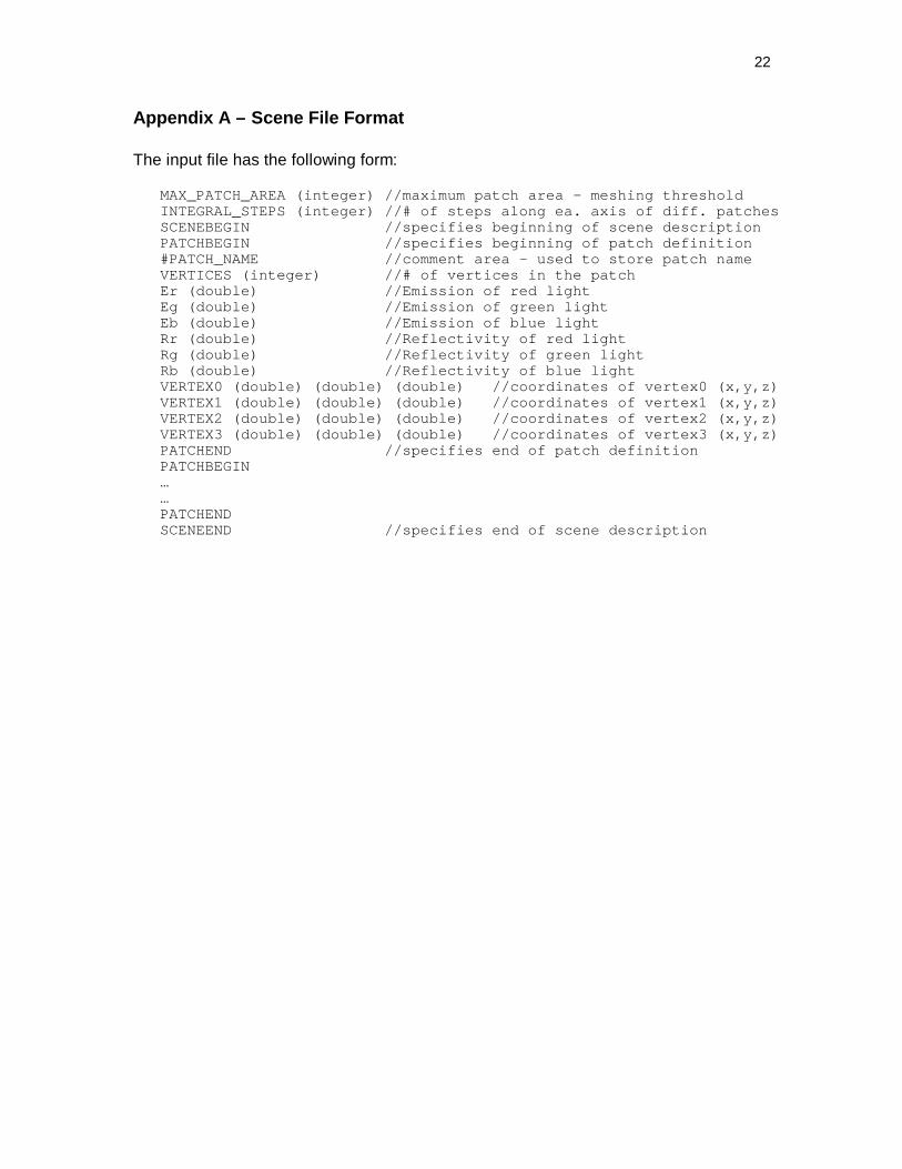
Appendix A – Scene File Format

The input file has the following form:

MAX_PATCH_AREA (integer) //maximum patch area – meshing threshold INTEGRAL_STEPS (integer) //# of steps along ea. axis of diff. patches SCENEBEGIN //specifies beginning of scene description PATCHBEGIN //specifies beginning of patch definition #PATCH_NAME //comment area – used to store patch name VERTICES (integer) //# of vertices in the patch Er (double) //Emission of red light Eg (double) //Emission of green light Eb (double) //Emission of blue light Rr (double) //Reflectivity of red light Rg (double) //Reflectivity of green light Rb (double) //Reflectivity of blue light VERTEX0 (double) (double) (double) //coordinates of vertex0 (x,y,z) VERTEX1 (double) (double) (double) //coordinates of vertex1 (x,y,z) VERTEX2 (double) (double) (double) //coordinates of vertex2 (x,y,z) VERTEX3 (double) (double) (double) //coordinates of vertex3 (x,y,z) PATCHEND //specifies end of patch definition PATCHBEGIN … … PATCHEND SCENEEND //specifies end of scene description

23

Appendix B – Color Plates

(color plate 1 – a test scene from my radiosity program – without smooth shading - computedcorrectly)

(color plate 2 – the same test scene computed by my program, rendered with smooth shading)

24

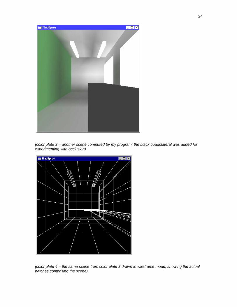
(color plate 3 – another scene computed by my program; the black quadrilateral was added forexperimenting with occlusion)

(color plate 4 – the same scene from color plate 3 drawn in wireframe mode, showing the actualpatches comprising the scene)

25

Appendix C – Program Listing

(attached)