Radiation pattern calculation for missile radomes in … The NPS Institutional Archive Theses and...
82
Calhoun: The NPS Institutional Archive Theses and Dissertations Thesis Collection 1996-09 Radiation pattern calculation for missile radomes in the near field of an antenna Herzog, Scott M. Monterey, California. Naval Postgraduate School http://hdl.handle.net/10945/32246
Transcript of Radiation pattern calculation for missile radomes in … The NPS Institutional Archive Theses and...

Calhoun: The NPS Institutional Archive
Theses and Dissertations Thesis Collection
1996-09
Radiation pattern calculation for missile radomes in
the near field of an antenna
Herzog, Scott M.
Monterey, California. Naval Postgraduate School
http://hdl.handle.net/10945/32246

NAVAL POSTGRADUATE SCHOOL MONTEREY, CALIFORNIA
THESIS
RADIATION PATTERN CALCULATION FOR MISSILE RADOMES
IN THE NEAR FIELD OF AN ANTENNA
Thesis Advisor: Second Reader:
by
Scott M. Herzog
September 1996
David C. Jenn Robert E. Ball
Approved for public release; distribution is unlimited.
co c:::::l c:=::>
c::T> C'-.1
•
\.''

REPORT DOCUMENTATION PAGE Form Approved OMB No. 0704-0188
Public reporting burden for this collection of information is estimated to average I hour per response, including the time for reviewing instruction, searching existing data sources, gathering and maintaining the data needed, and completing and reviewing the collection of information. Send comments regarding this burden estimate or any other aspect of this collection of information, including suggestions for reducing this burden, to Washington Headquarters Services, Directorate for Information Operations and Reports, 1215 Jefferson Davis Highway, Suite 1204, Arlington, VA 222024302, and to the Office ofManagemen~ and Budget, Paperwork Reduction Project (0704-0188) Washington DC 20503.
1. AGENCY USE ONLY (Leave blank) 2. REPORT DATE 3. REPORT TYPE AND DATES COVERED September 1996 Master's Thesis
4. TITLE AND SUBTITLE RADIATION PATTERN CALCULATION FOR 5. FUNDING NUMBERS MISSILE RADOMES IN THE NEAR FIELD OF AN ANTENNA
6. AUTHOR(S) Scott M. Herzog 7. PERFORMING ORGANIZATION NAME(S) AND ADDRESS(ES) 8. PERFORMING
Naval Postgraduate School ORGANIZATION Monterey CA 93943-5000 REPORT NUlvtBER
9. SPONSORING.tMONITORING AGENCY NAME(S) AND ADDRESS(ES) 10. SPONSORING.tMONITORING AGENCYREPORTNUlvtBER
11. SUPPLEMENTARY NOTES The views expressed in this thesis are those of the author and do not reflect the official policy or position of the Department of Defense or the U.S. Government.
12a. DISTRIBUTION/A V All...ABlllTY STATEMENT 12b. DISTRIBUTION CODE Approved for public release; distribution is unlimited.
13. ABSTRACT (maximum 200 words)
An analytical model and computer simulation are presented for a radome located in the near field of an antenna. Using the computer code described here, design tradeoffs can be performed between electrical, structural, and aerodynamic properties of the radome. The code is based on a method of moments solution to theE-field integral equation for bodies of arbitrary shape. Measured radiation patterns for AGM-88 High Speed Antiradiation Missile (HARM) and AIM-9C missile radomes are compared to computed data.
14. SUBJECT TERMS Radome, Method of Moments, PATCH.
17. SECURITY CLASSIFICA- 18. SECURITY CLASSIFI-TIONOFREPORT CATION OF THIS PAGE Unclassified Unclassified
NSN 7540-01-280-5500
1
19.
15. NUlvtBEROF PAGES _R-:t
16. PRICE CODE SECURITY CLASSIFICA- 20. LIMITATION OF TION OF ABSTRACT Unclassified
ABSTRACT UL
Standard Form 298 (Rev. 2-89) Prescribed by ANSI Std. 239-18 298-102

ii

Approved for public release; distribution is unlimited.
RADIATION PATTERN CALCULATION FOR MISSILE RADOMES
IN THE NEAR FIELD OF AN ANTENNA
Scott M. Herzog
Lieutenant, United States Navy
B.S.A.A.E., The Ohio State University, 1988
Submitted in partial fulfillment
of the requirements for the degree of
MASTER OF SCIENCE IN AERONAUTICAL ENGINEERING (AVIONICS)
from the
NAVAL POSTGRADUATE SCHOOL
Author:
Approved by:
Department of Aeronautics & Astronautics
iii

iv

ABSTRACT
An analytical model and computer simulation are presented for a radome
located in the near field of an antenna. Using the computer code described here,
design tradeoffs can be performed between electrical, structural, and aerodynamic
properties of the radome. The code is based on a method of moments solution to the
E-field integral equation for bodies of arbitrary shape. Measured radiation patterns
for AGM-88 High Speed Antiradiation Missile (HARM) and AIM-9C missile
radomes are compared to computed data.
v

ACKNOWLEDGMENTS
I would like to thank Professor David C. Jenn for his guidance and assistance
in undertaking this thesis. His expertise in radar and electromagnetics is truly an asset
to the Naval Postgraduate School.
Many thanks to Colin Cooper of the ECE Computing Staff for his high degree
of professionalism and assistance with the Suns workstations.
Most importantly I owe much gratitude to my wife and daughter, Holly and
Rachel. Without your infinite patience, support, and advice I would not have been
able to complete this project.
vi

TABLE OF CONTENTS
I. INTRODUCTION .................................................. 1
ll. ANALYSIS METHODS AND COMPUTER CODES ....................... 5
A. METHOD OF MOMENTS .................................. 5
B. RADOME WALL MODEL AND IMPEDANCE CALCULATION .... 9
C. PATCH AND RELATED PROGRAMS ....................... 15
D. RADOME PROGRAM .................................... 20
lll. COMPUTER CODE VALIDATION .................................. 21
A. APERTURE MODEL ..................................... 21
1. Patch Code Antenna Model . . . . . . . . . . . . . . . . . . . . . . . . . . . . 22
2. Radome Code Antenna Model . . . . . . . . . . . . . . . . . . . . . . . . . 29
B. SCATTERING DISK TEST CASE ........................... 29
IV. DATA ANALYSIS ............................................... 37
A. ANECHOIC CHAMBER FACILITY ......................... 37
B. PHASE CENTER FOR MICROLINE 56Xl HORN .............. 38
C. AGM-88 HARM RADOME ................................. 41
D. AIM-9C RADOME ....................................... 47
vii

V. CONCLUSION ................................................... 53
APPENDIX A. PROGRAM LISTING FOR IMPEDANCE CALCULATION ...... 59
APPENDIX B. SAMPLE INPATCH FILE LISTING ........................ 61
APPENDIX C. PROGRAM LISTING FOR VOLTAGE TAPERING ............ 65
APPENDIX D. PROGRAM LISTING FOR GEOMETRY COMBINING ......... 67
LIST OF REFERENCES .............................................. 69
INITIAL DISTRIBUTION LIST ........................................ 71
viii

LIST OF FIGURES
Figure 1.1 Ray tracing ........................ : ....................... 2
Figure 1.2 Spherical coordinate system . . . . . . . . . . . . . . . . . . . . . . . . . . . . . . . . . . . 4
Figure 2.1 Geometry for EFIE .......................................... 5
Figure 2.2 Stepped impedance transformer ................................ 9
Figure 2.3 Multi-layered radome wall geometry . . . . . . . . . . . . . . . . . . . . . . . . . . . . 11
Figure 2.4 HARM radome wall . . . . . . . . . . . . . . . . . . . . . . . . . . . . . . . . . . . . . . . . 13
Figure 2.5 AIM-9C radome wall . . . . . . . . . . . . . . . . . . . . . . . . . . . . . . . . . . . . . . . 13
Figure 2.6 HARM radome impedance as a function of incidence angle . . . . . . . . . . . 14
Figure 2.7 Relationships between PATCH and its pre- and post-processing programs
............................................................ 17
Figure 2.8 Plate composed of triangular facets ............................. 18
Figure 3.1 Microline 56X1 standard gain hom ............................. 21
Figure 3.2 Aperture model for Microline 56Xl antenna ...................... 23
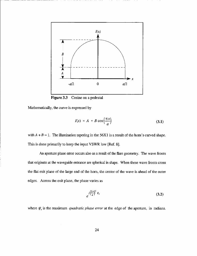
Figure 3.3 Cosine on a pedestal . . . . . . . . . . . . . . . . . . . . . . . . . . . . . . . . . . . . . . . . 24
Figure 3.4 Effect of tapering . . . . . . . . . . . . . . . . . . . . . . . . . . . . . . . . . . . . . . . . . . 26
Figure 3.5 Effect of quadratic phase error . . . . . . . . . . . . . . . . . . . . . . . . . . . . . . . . 26
Figure 3.6 Comparison of main beam E-plane patterns ....................... 28
Figure 3. 7 Comparison of main beam H-plane patterns . . . . . . . . . . . . . . . . . . . . . . 28
Figure 3.8 PEC disk in front of aperture . . . . . . . . . . . . . . . . . . . . . . . . . . . . . . . . . . 30
ix

Figure 3.9 Patterns with aperture and disk . . . . . . . . . . . . . . . . . . . . . . . . . . . . . . . . 32
Figure 3.10 Effect of antenna surface impedance on the aperture pattern . . . . . . . . . 33
Figure 3.11 Effect of antenna surface impedance on the aperture and disk pattern . . 34
Figure 4.1 HP X890A microwave horn .................................. 37
Figure 4.2 Anechoic chamber facility . . . . . . . . . . . . . . . . . . . . . . . . . . . . . . . . . . . . 39
Figure 4.3 Phase center adjustment . . . . . . . . . . . . . . . . . . . . . . . . . . . . . . . . . . . . . 40
Figure 4.4 HARM (upper) and AIM-9C (lower) radomes in anechoic chamber .... 41
Figure 4.5 HARM radome model . . . . . . . . . . . . . . . . . . . . . . . . . . . . . . . . . . . . . . . 42
Figure 4.6 Effect of varying aperture impedance . . . . . . . . . . . . . . . . . . . . . . . . . . . 44
Figure 4. 7 Effect of varying radome impedance . . . . . . . . . . . . . . . . . . . . . . . . . . . . 45
Figure 4.8 Comparison of measured and computed patterns for HARM radome . . . . 46
Figure 4.9 AIM-9C radome model . . . . . . . . . . . . . . . . . . . . . . . . . . . . . . . . . . . . . . 48
Figure 4.10 Effect of varying aperture impedance . . . . . . . . . . . . . . . . . . . . . . . . . . 49
Figure 4.11 Effect of varying radome impedance ........................... 50
Figure 4.12 Comparison of measured and calculated patterns for AIM-9C radome .. 51
Figure 5.1 Effect of HARM radome on antenna pattern ...................... 57
Figure 5.2 Effect of AIM-9C radome on antenna pattern . . . . . . . . . . . . . . . . . . . . . 58
X

I. INTRODUCTION
The radome is an essential part of communications and radar systems deployed on
aircraft. It provides environmental protection for the antenna and therefore must withstand
extreme aerodynamic and thermal stresses (such as on a supersonic missile) and must also
effectively transmit electromagnetic radiation. For example, the radome is a critical
component on an anti-radiation missile (ARM). An ARM uses a passive antenna to home in
on enemy radar emissions. The emitted energy passes through the missile's radome, which
has some loss and also introduces beam pointing error. The main beam's field of view (FOV)
must be narrow enough for proper target discrimination, but wide enough for off-boresight
intercept. The radome can also increase side lobe levels, which must remain low enough to
prevent azimuth and elevation errors. The result is degraded antenna performance when the
radome is present relative to when the antenna is operating isolated in free space.
Traditionally, aerodynamic, structural, and thermal requirements have dictated the
design of a radome, with the electrical performance taken as a consequence. The analytical
model and computer code described in this thesis can be used to optimize the overall design
of the radome since electrical design tradeoffs can be performed concurrently with the
aerodynamic and structural engineering. Therefore, an accurate analytical model of the
antenna and radome is required for efficient, cost-effective radome design.
There are basically two methods of analyzing radomes of arbitrary shape: (1) ray
tracing (geometrical optics), and (2) the method of moments (MM). For ray tracing, a
spherical wave is assumed radiated from the antenna, which is approximately planar at the
1

radome so that the Fresnel reflection coefficients can be used. Rays are traced from the
antenna to the radome surface, where reflections and refractions occur. The transmitted rays
are used to reconstruct an aperture distribution. The far field is computed using radiation
integrals [Ref. 1].
Ray tracing is only applicable for electrically large radomes that are in the far field of
the antenna. For low side lobe antennas, multiple reflections are important, and a significant
amount of bookkeeping is required to determine the ray trajectories. An example of ray
tracing is illustrated in Figure 1.1.
Transmitted rays
Radome
Ray tracing is approximate in the near field because:
(1) Rays are not parallel (2) Radome surface is not locally flat
Figure 1.1 Ray tracing
2

The computer code presented here uses a method of moments solution to the electric
field integral equation to calculate the effect of a dielectric radome shell in the near field of
an antenna. The method of moments is rigorous in that all multiple reflections between the
radome walls are included. As will be demonstrated, the code is flexible as well as accurate
and handles radomes of any shape and size (with size limited only by the available computer
memory).
Chapter II reviews the analysis methods and computer codes. An overview of the
method of moments is presented. Essentially the electric field integral equation is reduced to
a matrix problem which is readily solved by numerical methods. Also, the equivalent single
layer impedance is derived for multiple layer radome walls. The impedance is calculated for
two test radomes: an AGM-88 HARM and an AIM-9C. The impedance values are used by
the method of moments computer codes. Chapter II concludes with a discussion of these
codes. RADOME, a code developed by Francis [Ref. 2] and later improved by Klopp
[Ref. 3], is limited to bodies of revolution (BOR), and uses a thin-shell approximation for the
radome wall. In this thesis, a code developed by Sandia National Laboratories called PATCH
[Ref. 4] is applied to the radome problem. It represents the radome as a collection of
triangular patches which allows for virtually any geometry as well as various dielectric
materials. Cartesian coordinates describe antenna and radome geometry in PATCH, while
spherical coordinates describe the electromagnetic field. The coordinate systems are shown
in Figure 1.2. Typically the radome is oriented with the axis of symmetry coincident with the
z-axis.
3

,---------------------~--~------
Figure 1.2 Spherical coordinate system
Chapter ill explains the procedure used to modify and validate PATCH. An antenna
aperture model is developed for a standard gain hom that is used for both PATCH and
RADOME programs. A test case was run and the computed results from both programs are
compared to measured data obtained in the anechoic chamber. An additional test case is used
to demonstrate the capability of PATCH to accurately calculate multiple reflections.
Chapter IV presents the data obtained by analyzing the two test radomes. The
anechoic chamber facility is described and measuring techniques are discussed. Several
improvements have been made since the chamber's inception. Automated measurements are
made using a HP-8510 network analyzer linked to a personal computer.
Finally, Chapter V presents a summary of results and conclusions based on working
with the code as a radome analysis tool. Sources of measurement error are discussed and
recommendations are made to enhance the existing computer models and codes.
4

ll. ANALYSIS METHODS AND COMPUTER CODES
A. METHOD OF MOMENTS
The computer codes that will be discussed in the following sections use the method
of moments (MM) to calculate radome effects. A detailed discussion of this method can be
found in [Ref. 1]. Only an overview of the method is presented here.
The electric field integral equation (EFIE) is commonly encountered in electro-
magnetics. This equation relates the scattered electric field to the electric current on the
surface of an object. The EFIE is classified mathematically as a Fredholm equation since the
limits of integration are fixed (i.e., over the body). Because the unknown variable appears
only in the integrand, it is a Fredholm equation of the first kind.
To derive the EFIE, we first define the coordinate system shown in Figure 2.1. The
target, or scattering body, is assumed (temporarily) to be a perfect electric conductor (PEC).
PEC TARGET WITH SURFACES
X
~UB.RENT ELEMENT Js(r')
Figure 2.1 Geometry for EFIE
5
~ OBSERVATION POINT
-------- -------------------------

We will introduce a correction term later that will remove the PEC restriction. Note that in
general, S includes both the radome and antenna surfaces. We define
and the free-space Green's function as
G(rJ'> = e -jkR
4nR
(2.1)
(2.2)
After some manipulation [Ref 1, pp. 117-118], the final form of the EFIE suitable for
solution by a numerical technique is
Elan = J J {1 w~~(r')G(Y,r') - ~e [v' ·~(r)]v'G(Y,r')Ln~' (l.3) s
- -where Ei is the incident electric field, Js is the surface current density, ~ is the permeability,
E is the dielectric constant, and c..> is the angular frequency. Since the total electric field is the
sum of the incident and scattered electric fields, by imposing the PEC boundary condition
-(total tangential electric field is zero), Equation 2.3 states that the tangential component of Ei
equals the tangential component of the scattered field.
This form of the equation can be applied to any arbitrary surface. The incident field
is always known, and the surface current density is the only unknown. The incident field can
be a plane wave or an impressed voltage on the surface of the body. Potentials on the antenna
surfaces produce an electric field which then becomes the incident field on a scattering body
6

such as a radome. 'This interaction between the antenna and radome is embedded in
Equation 2.3.
The method of moments is a procedure used to reduce the integral equation to a
matrix problem. We start by representing the current in Equation 2.3 as a series with
unknown expansion coefficients, In.
(2.4)
The vectors ] n are known as the basis functions. These are either subsectional or entire
domain functions, and are chosen to be accurate representations of the current and
mathematically convenient (easy to integrate and differentiate). Typical subdomain basis
functions include impulse functions, rectangular pulses, and overlapping triangular pulses.
Entire domain functions include sinusoids and exponentials. A testing procedure is performed
in which both sides of Equation 2.3 are multiplied by each testing function and integrated over
its domain. Thus N equations are obtained, each with N terms. The simultaneous set of
equations can be cast into matrix form and when solved yield
I = z -lv (2.5)
where I is the vector containing the expansion coefficients, In . Z is an impedance matrix and
V the excitation vector. Generally both of these have complex elements. The specific form
of the elements depends on the choice of basis functions. The coefficients from Equation 2.5
7

are then used in Equation 2.4, which yields the surface current, Js. This in turn is used in the
radiation integrals to find the fields due to the surface current.
The mth element of the excitation vector V in Equation 2.5 has the form
vm = I I~·. Jm * ds (2.6) sm
where Jm * is the testing function and ~ the incident antenna field. sm denotes the portion
ofthe radome surface over which Jm * is nonzero. In general, the Sm can lie in the near field
of the antenna and therefore no far field approximations can be applied. The antenna models
in PATCH and RADO:ME differ, and both will be described later. Neither code has
restrictions on the location of the radome relative to the antenna.
Equation 2.3 applies to a perfectly conducting surface. For thin dielectric shells such
as radomes, the EFIE for perfect conductors is modified by adding a load term outside of the
brackets [Ref 1, p. 158]. This thin-shell approximation replaces the volume polarization
currents flowing throughout the dielectric with a thin sheet of surface current. The result is
that the elements of Z in Equation 2. 5 are also modified by the addition of a load term.
Overall, the method of moments provides a rigorous solution for the induced current
density on a body. When properly applied, the series representation for the current will
converge to the actual current as the number of basis functions is increased [Ref 1]. Since
the solution reduces to a matrix problem, :MJ\.1 is well-suited for computer coding.
Two :MJ\.1 solutions have been applied to the radome problem in this thesis. One
solution (RADOME) applies only to bodies of revolution. By exploiting the rotational
8

symmetry of bodies such as ogives and hemispheres, basis functions can be chosen that
reduce the number of linear equations that must be solved. The second solution (PATCH)
uses triangular subdomains, which are the most flexible for modeling arbitrary surfaces.
B. RADOME WALL MODEL AND IMPEDANCE CALCULATION
The impedance of a multi-layered (sandwich) radome can be calculated using a
stepped transmission line analogy. The impedance of the region on the exterior of the
Figure 2.2 Stepped impedance transformer
radome, ZL , is transformed through each layer until the region on the interior side is reached.
This transformed impedance, Zin , is the impedance that is presented to a plane wave incident
on the radome. The schematic representation of a sandwich radome is shown in Figure 2.2.
To apply the transmission line model to the radome, we first define the quantities shown in
Figure 2.3. Each layer n has a thickness, tn , and a relative dielectric constant, En • The
exterior region has the highest index and the interior region the lowest. The exterior is region
9

.-------------------~---------------------
number N, so there are N-2layers of radome material. Let TJn be the intrinsic impedance of
the layer n and zn be the wave impedance looking into the layer n at an incidence angle en.
For perpendicular polarization
(2.7)
and for parallel polarization
(2.8)
in is the transformed impedance that is seen looking through a sandwich of layers as shown
in Figure 2.3. The transformed impedance is
where as in [Ref. 5]
1 ~ n ~ (N -1)
r,:-;;i ( E ") J. Yn = a+jp = jwyp 0 .:/ 1- j--;J 2
10
E1 = E E 0 r
(2.9)
(2.10)
(2.11)
(2.12)

[• lz t t3 t •[• tN-1 •[ zl z3
lli ll3
Interior •••
Figure 2.3 Multi-layered radome wall geometry
The input impedance is computed by transforming the free space load of the exterior
back to the interior surface. An input impedance is computed at each interface and then used
as a load to be transformed back to the previous interface [Ref. 6]. This is repeated until in
is computed for the final layer.
The change in incidence angle at the interface between materials with different
dielectric constants (refraction) can be determined by using a form of Snell's Law. This is
expressed as
or
11
Tln - 8 -- sm n.
lln+l (2.13)

If necessary, an equivalent single layer radome (denoted by the subscript e) can be
derived from a multiple layer radome by using the equation
(2.14)
Since Z;n is complex, Ze and the product y /e can be determined.
Once known, the impedance Zin can be used to solve for the reflection coefficient seen
by an incident wave
p = z.- z zn o
(2.15) z. + z zn o
When Z;n and ~ are equal, p = 0, and all energy is transmitted. When there is a large
difference between Z;n and 4, , I p I .... 1 , and a large reflection results. Hence, the best
radomes have impedances that are close to the intrinsic impedance of free space,
approximately 377 ohms.
The PATCH and RADOME programsrequireradome impedance as an input parameter.
For a sandwich wall, the value can be calculated from Equation 2. 9. The impedance is allowed
to change as a function of position on the radome, but it is assumed constant with angle. Using
a computer program (see Appendix C) to calculateZin for a range of incidence angles, an estimate
of the radome impedance was obtained that was relatively constant over a broad range of
incidence angles. An average value of impedance was chosen for each of the radomes measured
and used in the computer simulations.
12

Two particular radomes were used for testing and analysis in this thesis: ( 1) an
AGM-88 HARM, and (2) an AIM-9C. The cross sectional geometry for the walls are shown
in Figures 2.4 and 2.5, respectively. The computer generated impedances for the HARM
radome are shown in Figure 2.6. The impedance is relatively constant over the range
0 o ::o: 8 ::o: 50 o • From the geometry of the HARM radome and the antenna, it was determined
Er = 3.5 1.2 3.5
Interior Exterior
(1) (5)
t (nun) = 1.37 3 0.7
Figure 2.4 HARM radome wall
(1) (3)
5.44 nun
Figure 2.5 AIM-9C radome wall
13

HARr.l RADOr.IE.Ir.I~E.DANCE. 2000 .-------.---r---,.-----r---r---.-----r---,
1:500 -;' E
. . . . . . . .. . -.- .. ~-.- ...... -.- -~ .... -.......... ~.-.- ....... -. . . . -·-··A· -............... -:-.- ............ -:- ................ ~ ............... . . . .
....
.e.1coo ;;; .. a:
:500 -.- ...... -.- !-.-.-.-.-.- .:.. . -.... -.-.-. ~.- ............ . .... V 0~-~--~--L--~--~--L--~--~
0 10 20 30 50 eo 70 eo
2000 .-----.---r---.-----r---r---.-----r---, 1:500 .......... ; ............ : ........................ ; ............ ; ........... ~ ........... ; ......... ..
• I I I : : I
1l 1000 : : : ' : : :
~ ·~ ••••••••,•••••••••,••••••••,••••••••••,•••••••••••~••••••r••;zv ll -SOC ........... : ............ i ............ j ............ :---·-----·--j·---------·i ............ ! ........ .
-1 CCC .__ _ __._ __ _,_ __ .__ _ __,_ __ _,__ __ .__ _ __,_ __ _,
Q 10 20 30 40 50 Allgl6 of llleld&llca (dag)
eo 70 eo
Figure 2.6 HARM radome impedance as a function of incidence angle .
that the average incidence angle along the surface of the radome was approximately 35°.
Thus, an impedance of 278 - j31 ohms was used in the computer simulations. For the
AIM-9C radome, the impedance calculation was simplified due to the presence of just one
layer and nearly normal incidence around the hemispherical surface. Using Equation 2.9, the
AIM-9C impedance was 234 - j166 ohms. The impedance values for both radomes are listed
in Table 2.1.
Table 2.1 Radome Impedance Used in the Computer Calculations
Radome Material Complex Impedance
HARM Fiberglass composite 278- j31 ohms
AIM-9C Alumina 234 - j166 ohms
14

C. PATCH AND RELATED PROGRAMS
The program PATCH was produced by Sandia National Laboratories in 1988
[Ref. 4]. It is a FORTRAN program that uses the method of moments to calculate
electromagnetic fields from scattering and radiating bodies. PATCH performs the
electromagnetic calculations, while a collection of pre- and post-processing programs are
available for generating, formatting, converting, and error checking the input and output of
the PATCH program. A brief description of each program is given in Table 2.2. The
programs and their relationships are shown in Figure 2.7. Most of the programs1 were
generated at the Naval Postgraduate School to allow automatic meshing of bodies built in
AutoCAD and to translate the meshed surfaces to PATCH input format.
During execution, PATCH reads an input file with geometry and calculation
parameters. Either of two commercial computer aided drawing (CAD) programs, AutoCAD
or ACAD, can be used to specify a shape. These programs are extremely versatile, and are
unlimited in the scope of geometries that can be generated. Files can be transferred between
the two using the IGES format. Whether the shape is generated in AutoCAD or ACAD, the
later program is used to construct a shell mesh, which is written in ACAD's "facet" format.
Meshing results in a discretized body composed of triangular facets. For example, a simple
rectangular plate is shown in Figure 2.8. The degree of fineness (or coarseness) of the mesh
is determined by specifying the number of facets, or edges, along the horizontal and vertical
1Commercially available program names are in ALL CAPITALS, locally generated programs are in boldface, and input/output files are in italics. Locally generated programs have various authors, and have been modified to suit individual users.
15

Table 2.2 Summary of PATCH and related processing programs
Name Brief Description Source
Auto CAD CAD drawing program Autodesk
ACAD CAD program capable of auto meshing Lockheed-Martin surfaces (Ft. Worth, TX)
pta.x PATCH-to-ACAD data translator NPS
atp.x ACAD-to-PATCH data translator NPS
knit.x Checks PATCH data files for duplicate edges NPS and nodes
bldmat.x Generates MA TLAB ".m" files for plotting NPS geometry using PATCH data files
pltpatch.m A MA TLAB program that plots the geometry NPS files generated by bldmat.x
combine.m A MA TLAB program that combines separate S.M. Herzog geometry files into one object for use in PATCH
BUILDN5.X PATCH preprocessor to generate input Sandia National geometry files and specify calculation Laboratories parameters
PATCH Numerical electromagnetics code that Sandia National (patch2v.x) computes scattered and radiated fields using Laboratories
the method of moments.
sides. As a rule of thumb, the lengths of the individual edges should be approximately one
tenth of a wavelength (0.1 J.. ). For larger bodies, this means a large number of elements, and
a correspondingly larger facet file.
The facet file generated by ACAD must then be converted to PATCH text format.
This is accomplished by the program atp.x (ACAD to PATCH). The program pta.x
performs the reverse data translation. The PATCH version of a facet file defines the
16

.------....;--~~ knit.x
Geomet:Iy Definition
atp.x ACAD ptax
l ! AutoCAD
buildn5.x HPostscriptfile] ....---
~--~BLDMAT~~~~
inpatch ~
r!.ATh2CH H outpatch ) t-Yatc v.x
----- ---- .. I
I
L.-----.&..•1 ~pltpatch.m
I
I I
I_ - - - - - - - - - I
MATLAB
Figure 2.7 Relationships between PATCH and its pre- and post-processing programs
17

.----------------------------------
.. . .. ..
Figure 2.8 Plate composed of triangular facets
geometry in terms of nodes and edges. Nodes are listed with their respective Cartesian
coordinates, and edge segments are listed with their two defining nodes. An example of this
will be presented later. The output of atp.x is used in the program BUILDN5.X, which
constructs the final ASCIT input file that PATCH will read. When BUILDN5.X is executed,
it prompts the user to specify the input geometry file, which is the converted facet file from
atp.x. If no input file is available, simple geometries such as quadrilaterals, disks, or spheres
can be generated by BUILDN5.X. The program then asks for a set of simulation parameters
that define the particular calculations to be performed. At this point the excitation voltages
and currents, surface impedances, frequencies, and observation points are entered. The
program BUILDN5.X compiles all of this information and constructs an AS CIT file properly
18

formatted for use in PATCH. This file must be renamed inpatch before PATCH is executed.
A sample inpatch file for the mesh in Figure 2.8 is listed in Appendix A. The program
BUll..DN5.X is also capable of displaying the geometry on the screen or writing a postscript
file. However, geometry display requires the DISSPLA graphics software package.
When PATCH is executed, a number of output files are generated. Outpatch is a data
summary that includes a listing of all the input parameters, geometry (nodes and edges), and
the computed fields and currents. Three additional files, ampp.m, ampt.m, and ang.m are
saved with .m extensions for use in MA TLAB. These files contain the calculated radiation
pattern data, as noted in Table 2.3. MA TLAB is the primary means by which the calculated
pattern data is displayed. The .m files are simply loaded into a plotting routine to view the
data points.
Other PATCH related programs include bldmat.x, knit.x, and combine.m. The
program bldmat.x enables a display of the mesh model in MATLAB. The program converts
the ASCII facet file (from atp.x or BUILDN5.X) to .m files. The MATLAB routine
pltpatch.m is then used to display the geometry. Combine.m appends one geometry file to
another so that successive nodes and edges are numbered in sequence.
There are occasions when the facet files generated by ACAD/AutoCAD contain
redundant points or edges. The program knit.x is an error checking routine that removes
duplicate edges and checks for other file errors. This program provides a means to remove
bad data and generate a new error-free data file.
19

D. RADOMEPROGRAM
The FORTRAN program RADOME is used to compute the pattern of an antenna
radiating in the presence of an axially symmetric radome. This code also uses the method of
moments, and was originally developed by Francis [Ref. 2] and later improved by Klopp
[Ref. 3]. See also [Ref. 7]. The code is essentially self contained and does not require the
geometry preprocessing that PATCH does. RADOME is restricted to axially symmetric
bodies of revolution (BOR) such as cones, disks, spheres, hemispheres, paraboloids, cylinders,
and ogives. These basic shapes can be generated internally by RADOME. Other generating
curves can be specified in the file radinp, which is simply a two-column table of surface
coordinates p and z. RADOME produces three output files that are saved with a .m file
extension for plotting in MATLAB (see Table 2.3). For bookkeeping purposes, the
underscore character in the filenames is occupied by a letter character that identifies the run.
Just as in the case of PATCH, each observation angle in ang_.m has a corresponding pattern
value in eppol_.m and etpol_.m.
Table 2.3 Output files for PATCH and RADOME
PATCH RADOME Description
output files output files
ang.m ang_.m Azimuth observation angles (8 points)
ampp.m eppol_.m E<P (<!>-polarized E-field component, in dB)
ampt.m etpol_.m E6 (8-polarized E-field component, in dB)
20

ill. COMPUTER CODE VALIDATION
A. APERTURE MODEL
In order to validate the results of the PATCH and RADOME programs, we need to
accurately model the antenna used in the anechoic chamber measurements. Details of the
chamber facility are discussed in Chapter IV. For all of the experimental data that was
gathered, a Microline 56Xl Standard Gain Horn was used as a receive antenna. This horn
has an exponential taper in both theE- and H-planes as depicted in Figure 3.1. Typically, this
type of horn is used in the detection and measurement of microwave power. Additional
specifications for the horn are given in Table 3.1. The low voltage standing wave ratio
(VSWR) is crucial to laboratory measurements since it prevents undesirable reflection at the
TOP VIEW
SIDE VIEW
DRAWING NOT TO SCALE
Figure 3.1 Microline 56X1 standard gain horn 21
All units in em

antenna input which could possibly add constructively or destructively with radome
reflections, thereby producing misleading data.
Table 3.1 Microline 56Xl Specifications
Frequency Nominal Frequency at Gain Variation over Accuracy Maximum VSWR
Range Gain Nominal Gain Frequency Band
8.2-12.4 GHz 17 dB 11.0 GHz +/- 1.5 dB +/- 0.3 dB 1.15
1. Patch Code Antenna Model
In order to simulate the 56Xl horn in PATCH, a model of the antenna aperture was
developed based on slots in a conducting sheet. The excitation amplitude of the slots is
obtained by sampling the TE10 mode distribution which is approximately the distribution in
the horn aperture. A rectangle approximating the size of the actual horn aperture (5.4 x 7.3
em) was subdivided into a 12 x 13 grid of smaller squares, which in turn were divided into
two faces by the addition of a diagonal. At 10 GHz, which is the test frequency for all
measurements, the smaller squares are 0.2A (0.6 em) in dimension. This allows the individual
element to be electrically small while keeping the grid from becoming too dense. The
aperture grid is shown in Figure 3.2.
The next step is to determine the voltage excitation at each slot. If a voltage is applied
across a small horizontal slit in a conductive material, the resulting far field pattern will have
22

I" !'. "' ~ ~ I~ ""' ~ I" ~ "' ~ I" 0.03 I" I" ~ ~ I~ I'S_ "' ~ I" ~ "' ~ I" I" ~ " I~ "' ~ ~ 1\._ "' 'S ~ ~ "' 0.02
I" """ """
~ I" " ·~ I" ~""" I" I~ " I~ """ ~ i" I~ """ ' I" 'S-"""
0.01
~ ~""" I\_ "' ~"'- ~"'
,, I" ~"
I" ~"' I\_ " ~I" I~ " I~ I" ~" I" ~ ""' !\_ " ~ I\._ " ~ I" ~ """
;;; i 1 Q
> -0.01
I" I~ " I~ " ~~"' I~ " ~ I" 'i "' I" IS. "' I'S-"' ~ 1'\ " ·~ I" ~ " -o.a2
I" I~ " I~ "' ~~"' I~ " I~ I" 'i " I" IS. "' I'S_ "' ~ ~ ~ " ~ ~ 'i """ .o.a• .C.a.& .0.03 .0.02 .C.OI 0 0.01 0.02 0.03 C.C4
X(mGt.,.)
Figure 3.2 Aperture model for Microline 56Xl antenna
a vertical E-plane (y) and a horizontal H-plane (x). An array of slits with varying voltage
amplitude and phase excitations can be used to control the array far field pattern
characteristics. The larger the array becomes in the horizontal direction, the narrower the H-
plane beamwidth. And conversely, the larger the array in the vertical direction; the narrower
the E-plane beamwidth. For the Microline antenna model, a total of 72 horizontal edges were
chosen as slits. These are denoted by small dots in Figure 3.2. The extra row of squares at
the top is required to specify the polarization of the slits just below. The size of the aperture
and the pattern of slits were adjusted until the computed pattern agreed with the measured
56Xl pattern in gain and beamwidth.
Because ofTE10 waveguide excitation imperfections and the hom flare, the aperture
plane of the 56Xl does not have uniform illumination with constant phase. The actual
illumination can be modeled by a cosine on a pedestal function as shown in Figure 3.3. The
pedestal value, or illumination present at the edge, is A, and the width of the aperture is a.
23
~-----------------------------------------------------
l(x)
~--------
B
~--+--------- ---------A
-L--~----------~------------~~x
-a/2 0
Figure 3.3 Cosine on a pedestal
Mathematically, the curve is expressed by
l(x) = A + B cos ( 1tx) a
a/2
(3.1)
with A+ B = 1. The illumination tapering in the 56Xl is a result of the horn's curved shape.
This is done primarily to keep the input VSWR low [Ref. 8].
An aperture phase error occurs also as a result of the flare geometry. The wave fronts
that originate at the waveguide entrance are spherical in shape. When these wave fronts cross
the flat exit plane of the large end of the horn, the center of the wave is ahead of the outer
edges. Across the exit plane, the phase varies as
(3.2)
where lfrx is the maximum quadratic phase error at the edge of the aperture, in radians.
24

Together, the cosine taper and phase error produce an illumination in the horizontal direction
which is expressed as
1tX j- 1/Jx
] (2x)2
I(x) =[A + Bcos(-;-} e a • (3.3)
Tapering in the vertical direction is expressed by substituting y for x and b for a in Equations
3.1 through 3.3. Since the taper and phase error in the vertical direction is not necessarily
the same as the horizontal direction, the constants A and B will not be the same, and lf!x will
be replaced by 1/ly •
Applying the illumination function to the aperture model, Equation 3.3 is sampled at
the slit locations to obtain the array excitation. Different values for the pedestal and phase
error were investigated until there was satisfactory agreement with the measured 56X1
antenna pattern. A program for defining a two-dimensional tapered array of voltages is listed
in Appendix B. The effect of increasing the taper (B >A) is to reduce the side lobe level and
increase the beamwidth. The effect of increasing the phase error is to fill the
pattern nulls between the main beam and side lobes. Beamwidth is not significantly affected
for small values of lf!x. The pattern effects are illustrated in Figures 3.4 and 3.5.
After numerous iterations, the best agreement with measured data from the 56X1 horn
occurred withE-plane taper values of A= 0.6, B = 0.4, and rfrx = 35° (denoted by 0.6/0.4/35°).
The corresponding best H-plane parameters were chosen as 0.1/0.9/70°. The patterns for
both planes are shown in Figures 3.6 and 3. 7. The agreement is good in the main beam, with
25

Effect of Taporlng Aportllro {E.-Plano)
:J>haco Error: SS !l~g . . . . . .
-5 ····:··· .. ······: .. ·········:···········:
-10
iii :!!:-.15 c
Cii Cl
-20
-25
-eo
Figure 3.4 Effect of tapering
-20 0 20 Th6Til. {dog)
-;.11.11 ·::::.·!.!i.i" ..
:.5/.5
eo eo
Effect ai Quadra11c: Pllase Errcr (E-Piane)
:E.-plano I!'P<>r: 0.8!0.4 . . .
-5
-10 ---~----------~ ........... ~-----··
iii :!!:-.15 .... , ........... ; ........ . c Oi CJ·
-20
-25
-30 .... ; ......
-80 -80 -40
Phaco E.nor
: ~Od.ag . -:--......... , ..... :.:·.::r:ia·d~--:- --
-20 0 20 Thota {dog)
. ~ 40 dGg ~
....... L .. ::-::~~.o.r;~.~-~ ..
0 180!1Gg 1
40 ec 80
Figure 3.5 Effect of quadratic phase error
26

- -----------------~~~~-
about 2 dB difference in the side lobe level for PATCH. This is to be expected due to the
sampling nature of the model itself. For the simulations using radomes, the aperture model
described above is used as a reference. By comparing these patterns with those obtained with
the radome present, the effect of the radome can be deduced.
27

.----------------------------~·------ ------
E-PiaM Pa!l.m Cemparlscn 0.-.-----.---~--------~~--~----.-----r---~~
PA"f:CH tapor!ra11o {AI~): 0.1!10.~ PAT.-cH pllaseenDr: 35 de9 ; j-- PATfH RA~Ot.IEtapierrade (~): 1.C~.a . '. , ;... _ RAO:OME RA~Ot.t E ph=;aso orrer::5C dag ; ; l, ; ; ;
-5 '"1"""""'~"'''''"'';"······-r ....... r ...... ~-~ ......... r····"·t.t-~~Jiod ... : : I
= : . . . . . ~-tc ... f ....... T ....... T ............. T........ , ...... f .......... [ ....... ..
.5 .. Cl
-15 }········ ··))/•;:~; + . . .L .... "· :::::tf>:········· !/,': : ~\\\;
~. , ! I , , ; , ; I , \ 40
. ·: >;"/ ' . ' T T f \j\ .. ~ : : ,:
-ea -sa -40 -2C a :2a I!C ea Theta (deB)
Figure 3.6 Comparison of main beam E-plane patterns
H-Piulo Pattom Comparlscn Cr-.-----.---~----.---~~--~-----.----.---~--,
PAT:CH taper;ra11o (AI~): 0.110.1) PAT,.CH pllas. orror: 7~ dog ; _ PAlCH RAQOME tap:&rra11o (.lt.IB): a.t~.1 RA~Or.IE ph~o orror?O d09 ~ j . . ;-- RA~OI.IE
-5 .... ; ......... ; .......... ; .......... ;; ......... ; ........ ; ......... ~--..:'-"Vaij:ciired'"
: : ; i : : ~;...' -----+; -----+-' : : . :
. . : ~
-tO .... ; .. ......... ; ........... : .. ..... , ·:· ....... ... : ......... ~.! ......... : .......... :..... .... .. .
! ! ; ! ! ! •I ! ; : : ~ ~ .\
: ~ I, . . ... .: .......... ..:. .......... ::. ........ ..:. .......... :.. ......... -:. .................................. . . . . . . ; ,, .
·"
~ ···t·········-···}A········t········· f·········i······\J\.\····1········· ... -2S ... : .......... -:-. i ....... ~ ......... -:- .......... ~ ......... '!' .......... ~ .. T"i ('~ ....... ..
-110 -SO -40 -2C a :2a nota (dea}
Figure 3. 7 Comparison of main beam H-plane patterns
28
80 110

2. Radome Code Antenna Model
The code RADO:ME can handle circular or rectangular antenna apertures of arbitrary
illumination. The antenna pattern is computed by integrating the specified distribution at a
given spherical coordinate location (R, (}, ifJ). No approximations are made in the calculation
other than numerically evaluating the integrals.
When using a rectangular aperture, the RADOME program asks for the antenna
dimensions in wavelengths. At 10 GHz, the 56Xl horn is 1.8 x 2.4 wavelengths. In order
to match the output with the measured data, the dimensions and distribution were adjusted.
As in the PATCH model, the program was modified to accommodate tapering and quadratic
phase error. The beamwidths were matched in RADOME using an aperture of 2.0 x 2.6
wavelengths. The values used for A, B, and lfrx, respectively, are 1!0/50° for the E-plane and
O.l/0.9noo for the H-plane. The resulting patterns are shown in Figures 3.6 and 3.7. There
is good agreement with the 56Xl measured data. Furthermore, for the purpose of radome
evaluations, there is satisfactory agreement between the patterns produced by RADOME and
PATCH. This demonstrates that when modeling the same antenna with both programs, there
is some correlation in the required tapers and phase errors and similar results are achieved.
B. SCATTERING DISK TEST CASE
The data in Figures 3.6 and 3.7 show that both the RADOME and PATCH antenna
models agree with measured data when radiating in free space. When a radome is present,
some waves scattered by the radome can return to the antenna and be either received or
29

rescattered. This interaction between the antenna and radome can affect the side lobe level
of the transmitted field, especially at wide angles. The RAD0:~1E code does not include these
multiple reflections between the antenna and radome, but PATCH does. The strength of the
antenna reflection in PATCH can be controlled somewhat by varying the surface impedance
on the aperture array plate.
A good test case for evaluating the effects of multiple reflections is to place a perfectly
conducting (PEC) disk in front of the aperture and compare the results for both codes. The
geometry is shown in Figure 3.8. The diameter of the disk is 2.A., and it is positioned 5.A. in
front of the aperture.
0.14
0.12
0.1
0.02
Q
Q
X(m) Y(m)
Figure 3.8 PEC disk in front of aperture
The resulting patterns are shown in Figure 3.9. The patterns from the main beam up
to the fourth side lobe agree very well (0 < fJ < 80°). The PATCH array plate impedance is
10,000 ohms, which makes it essentially invisible to fields scattered from the disk. Beyond
30

8= 90°, PATCH gives a number of additional lobes due to the disk scattered field adding and
canceling with the array field. RADOME has no antenna field in the rear hemisphere, and
thus the pattern in this region is determined solely by the disk scattered field. Figure 3.9
indicates that interactions between the antenna and disk are not significant in the range
oo < 8 < 9(1 , which is expected because the antenna models are transparent to waves
scattered from the disk.
In order to test the multiple reflection effects, PATCH was run with different impedance
conditions on the aperture plate. The surface impedance of the aperture was varied from 1 ,000 to
20,000ohms, with and withoutthediskpresent. Forthefirstcase (aperture alone), theresultsare
showninFigure3.10,ThereisvirtuallynochangeintheH-planepattern,andonlyasmallchange
in theE-plane pattern when the aperture surface impedance is varied.
The second case has the aperture with the PEC disk. Again the surface impedance of the
aperture plate was varied, and the resulting patterns are shown in Figure 3 .11. This case is more
interesting in that the surface impedance of the aperture is important with regard to multiple
reflections between the two structures. The patterns show that the aperture is relatively
transparent for impedances of 1 ,000 to 20,000 ohms, demonstrated by the fact that these curves
are grouped together. When the aperture is a PEC, we see the pattern diverges from the others as
a consequence of waves being reflected back and forth between the aperture and disk.
In summary, the PATCH code allows a wide range of antenna surface impedances which
directly affect the strength of the interaction between the antenna and scattering body.
31

E-Pian& Pattarn (ApGrturG and Disk)
-10
-20
.............. ~···-·· .... ··:- ....... . . . . . . . . . . . . . . 0 0 0 0 ..... , . ·:·- .... -·- .... :· ......... -.... : ............... ·: ............ . -40 .. . .. • -.- ... ·!- .... -.- ...... ·:- .............. ! ........ 0 ...... -~
I I 0 I • 0 • • • 0 • •
I I I I I I I I • • • 0 • 0 • •
I I I I I I I I • • • 0 . . . . I I I I ' . ' . . . . 0 0 0 .......................................................................... . . . . -.......... -.... -............................ -·· .................... . -50
I I I I . . . . I I I I . . . . ' . ' 0 0 0
' ' ' 0 • 0
-SO~-·~--~-~--~·-~·~·-~·~--~--~-·~-~--~·-~--~·-~·~-·~-~--~-~--~--~--~--~-~-~--~~~~~~~~~~~~~~~
0 20 40 so eo 100 120 140 ISO 180
H-PianG PattGrn (ApGrturG and Disk)
-10
-20
iii' "Cl ' . -;-30 ............. -~- ................. 0... •• • .. .... ,.,, ........................... --~-- 0 .. 0 ..... . . . . . . . . . . . 'ii 0
I I 0 I I . . . . . 0 0 I I I . . . . . 0 I I 0 I . . . . . 0 I I 0 0
-40 .. ·-·-···-·:-·-·- ....... ··:· .............. : ............... -~ ............... -:·· ............ ·-:· ............. ~--·-·· .... -·:-·-·" ...... . : : : : : . --i-- PATC~ I 0 I 0 0 0 0 . . . . . . . . . . . . . . . . . . . . .
-50 -Disk- DlamGtGr~-2~~ ·- · -· -·- · -:- ·- · · ·-·-·-:- ·-· -·- ·-· .; ..... -·-·-·~·- ·-·- · -~;-... ·RAD0ME-· -·-· Dlst. fram ApGrtu~G: 5"1 ~ ~ Disk: P.EC : , : :
-SO _ ApGrtur· : .. to .. no.a:..ctlms .... : ........... : _. _. _. _ .•. _: ....... -·-. : __ . -·- .•.•. : .•. _. _ ... __ :. _. _. _. _.
o 20 40 so eo too 120 t4o tso teo ThGta (deg)
Figure 3.9 Patterns with aperture and disk
32

-10
-20
iii" "'Cl
;-30 «< 0
-40
-50
-10
-20
iii" "'Cl ';-30 "iii 0
-40
-50
-E!C
E-Piane Pattern (Aptu1Ure Only)
-·-·!······-···· : ............... -:·-.- ....... -. -: ... 0 ... -.-. ~ ....... -.- .... : .... -.- ...... -:- ... .
; : : \ : : . . . . . I I I I I . . . . .
-' . . :~;.;··:·~ .... ~- ...... ~ ............... -~- ... . . ~.-..; . .
.. ' . ;::,;l· . . ... . ......... "' ... ·1· .... ' ... >:k:.i~ .. . ......... - ·:- ............... ~- .......... - ... ! .. 0 ............ -:· ...... -.- .... ~--.- ...... 0 ... ~.- .......... - -~.- ........ -~-.-.
I I I I I . . . . . I I I I . . . . I I I I
-eo -SO -40 c 20 40 so eo
H-Piane Pattern (Aper1Ure Only)
. . ..... ·:- ............... ·:- ............... ·:-.- ........... ; ............ -. -:·- .... -.- .... -:· -.-.- .... i.-.-.- ... 0 ... ~.-.-.- ...... ·:- ... . . . . . . . . . 0 0 I I 0 I 1 . . . . . . . 0 I I I I I I • 0 • • • • • I I I I I I • 0 • • • •
I I I I 0 I I ....................... : ............... · ................ .: .............. ; ............... :. ................ · ..... . I I I I 0 0 I . . . . . . . . . . . . . . . . . : ; -:- 1CCC al'lms ; ; ;
-·-+·-·-· ~~~·-·-·-·-·+···-·-· ·+·-·-·····+-···-·-·-+ ·-·-·-···!·-·-·-···- : ·-~ ~ · ~ ·- 5000 ~hmc ~ ~ I I I I I I . . . . . . I I I I I
......................................... , ............... 1 ................................. ., ..................................................... .
~ ~ ~ ·~ 1 c .ceq ohms ~ ~ ; ~ I I I 0 I I 0 I . . . . . . . . I I I I I I I I . . . . . . . I I I I I I I I -·- ·: ·- ·- ·- ·- ·- ·:- ·- ·- ·- ·- ·- :- ·- ·- ·- · .:.: ~-- 2"c-.croq· ~;Jur.-c ·- · :· ·- ·- ·- ·- ·: ·- ·- ·- ·- ·- ·: ·- ·- ·- ·- ·- ·:- ·- · 0 I I I I I I I
T2perratlo{AIB):0.1m.o ~ ~ ~ ~ ~ --~~":~~-~~~~!::??.~~~-- : __ -·-·-. -·-. -· -·-···- .: ... -·-· -·-· · ........... :. -·-·-· -·- ... -. -·-.-.- _: ___ . -eo -SO -40 -,20 c 20 40 so eo
Theta (deg)
Figure 3.10 Effect of antenna surface impedance on the aperture pattern
33

-10
-20
iii "Cl
;-30 Ill 0
iii "Cl
-40
-50
-10
-20
';-30 'i 0
-40
-50
-80 0
E-Piane Pattern {Aperrure a Disk)
20 40 80 80 100 120 140 180 180
H-Piane Patmrn {Aperrure a Disk)
' ' ............................................ ' ' . . ' ' . . ' ' . . ' ' . .
: ll I : I --~ PEC
' ' ... -.-...... .... . .. . .. . .. . .. . .. .... . .. . ... .. .... -.... -.- .............. -.... -·· ....... -.... -. .,, .......... -.... -........... -.... -.... -... . 0 I I I I 0 I I I . . . . . . . . I t I I I I . . . . . . I I I I I I ' : 1000 ohms . . . . . . I 0 I I I I
• • 0 0 • •
I I 0 I I I I
-·-·-·-·-·:·-·-·-·-·-T·-·-·-·-·-~-·-·-·-·-·-:··-·-·-·-·-~·-·-·-·-·-·y-·-· :..:·:..·~·2ci.cciic~m·c·-·-·
Taper ri1.11o {A/B):: 0.110.9 : ~ ~ : ~ ~
-~~~~~ .e!~~!: ?~.~~~---·-.-.-:-. -·-·-·-· _:-.- ·-·-. -· _:_-.- ·-·-·-. ·.-. -·-·- ·- ... -·-.- ·-.-: . -·-·-·-· 20 40 80 80 100 120 140 180 180
Theta {deg}
Figure 3.11 Effect of antenna surface impedance on the aperture and disk pattern
34

35

36

--------
IV. DATAANALYSIS
A. ANECHOIC CHAMBER FACILITY
The Naval Postgraduate School's anechoic chamber was used for all measurements
presented in this thesis. The chamber is approximately 25 feet long, 12 feet wide, and 10 feet
high. A Hewlett-Packard X890A microwave horn serves as the transmit antenna at one end
of the chamber. The geometry of this E-plane sectoral horn is shown in Figure 4.1. A
rotating pedestal is located approximately 19 feet from the transmit antenna. The pedestal
holds the receive antenna (Microline 56X1) and test radome, and is capable of rotating
3.05 em
Figure 4.1 HP X890A microwave horn
through 360° in azimuth. Both of the antennas are fed by coaxial cable via WR -90 waveguide
adaptors. The chamber walls, floor, ceiling, and pedestal are covered with carbon-based radar
absorbent material.
37

The measurement system uses a microwave amplifier, synthesized sweeper, frequency
converter, and network analyzer to generate, detect, and process microwave signals. The
pedestal servo motor and network analyzer are connected to a personal computer that serves
as the main controller/interlace for the chamber. A schematic of the chamber equipment is
shown in Figure 4.2.
Measurements were taken for -90° ~ {}~ 90°, with 0= 0° pointing directly at the
transmit antenna. Data was not recorded for angles beyond {} = ±90°, since the receive
antenna faces the rear of the chamber in this sector. In practice, the radiation pattern will be
close to zero because of the missile body. Using Labview 3.0 software to control the
instrumentation, data was recorded for a transmit frequency of 10 GHz at 1 o increments. The
recorded signal is an average of 32 samples taken at each azimuth angle. Sampling reduces
the effect of noise and provides more repeatable data.
B. PHASE CENTER FOR MICROLINE 56Xl HORN
In the far field of a microwave horn antenna, it is desirable to assign a reference point
for a given frequency such that the phase of the radiated wave is independent of {}and ifJ.
This point is called the phase center of the antenna. When viewed from a far field observation
point, the wave fronts radiated by the antenna are spherical waves that appear to originate
from the location of the phase center [Ref. 9].
A graphical method of obtaining the phase centers forE- and H-plane sectoral horns
is given in [Ref. 9]. For a given frequency and flare angle, the phase center distance is
obtained from a graph. An average flare angle was determined for the E- and
38

Transmit Receive
Anechoic chamber
Coaxial cable 20 dB direct
coupler Coaxial cable
20 dB attenuator
Variable attenuator
Coaxial cable
0 386 PC Labview 3.0 MS Windows 3.1
Motor controller
HP8348A microwave amplifier
2-26.5 GHz
HP83631A synthesized sweeper
HP8511 frequency converter
HP8510C vector network analyzer
IEEE488 GPIB/HPIB interface
RS232 serial line
Figure 4.2 Anechoic chamber facility
39
Coaxial cable

H-planes of the exponentially tapered 56Xl horn. Phase centers were then obtained for the
horn using the graph in [Ref. 9]. Using these estimates, the antenna model used in PATCH
was offset from the physical aperture plane (i.e., the location of the horn aperture when
measurements were made) by the phase center distance. This adjustment is shown in
Figure 4.3.
Radome Phase center
Hom
Aperture plane~ ~ Locate PATCH antenna 1 model here
Figure 4.3 Phase center adjustment
TheE- and H-plane phase centers are an approximation since the 56Xl horn is not
a true sectoral horn in either plane. To obtain the best phase center location, the PATCH
antenna model was stepped through different locations about the initial estimate until the
calculated antenna patterns converged to the measured patterns. This location was then
deemed the phase center for a given plane. The final values for the 56Xl antenna are 0.0 em
for theE-plane and -3.0 em for the H-plane. In other words, theE-plane phase center is
coincident with the hom aperture, while the H-plane phase center lies 3.0 em behind it.
40

-- --------------------------------------------,
C. AGM-88 HARM RADOME
Pattern measurements were made on an AGM-88 High Speed Antiradiation Missile
(HARM) radome that was mounted on the chamber pedestal in front of the Microline 56Xl
antenna. This set up is shown in the upper part of Figure 4.4. The position of the antenna's
aperture plane relative to the radome was noted so that an adjustment to the horn's phase
center could be made in the computer model.
A computer model for the HARM/56Xl antenna configuration mentioned above was
generated, and is shown in Figure 4.5. The antenna model was located at theE- or H-plane
phase center for each respective pattern calculation.
Figure 4.4 HARM (upper) and AIM-9C (lower) radomes in anechoic chamber
41

Before a comparison of calculated results with measured data can be made, it is
important to examine the effects of both radome and aperture impedance on the computer
generated results. First, the effect of varying aperture impedance was examined. This is the
impedance of the rectangular aperture plate that was used as the model for the Microline
56Xl antenna. Figure 4.6 shows theE- and H-plane patterns for aperture impedances of 100,
500, and 10,000 ohms. TheE-plane pattern shows the most change. As impedance is
increased, the side lobe peaks tend to migrate toward the center ( {} = 0°) and the main beam
narrows approximately 5° at -10 dB. Side lobe levels in the E-plane are decreased with
increasing aperture impedance. The H-plane pattern shows relatively little change with
increasing aperture impedance. The main beam shows virtually no change, and side lobe
levels are not significantly affected. There is some movement toward the center (as in the
0.2
!l.lll
O.IS
0.14
0.12
"E ;; C.l
0.011
o.os
0.04
C.02
a .Q .I
. . .. -• ~ - • - ' •••• ·:· 0 •• - •• - • ~ ••
. -... L .. -.--. ·.~.-.- .. -. ~-.-.-
; .. -·-····:-· .-· ·r· . -. -. -~- . -. -. -. : . -. -.
... :-····· r .-·.
~ . -.. -. _;_.-.- ...... ~.- ...
.. : ....... ~- ....... -
.... -:~: .
0.1 0.1
Figure 4.5 HARM radome model
42
-~-- ...
-. -. -~- ....
-... -~-- ... -'.
. .. -:·- ·-.
... ·~-- ·- ....
. - -~---- .....
·- ·:· ·-. 0
... -~-- ·-.-
-0.1
X{m)

E-plane) in the second and third side lobes. Thus, the value of aperture impedance determines
how transparent the antenna is to waves reflected and scattered back from the radome.
Figure 4.6 shows that the effect of aperture impedance on the HARM/56Xl model is minimal.
There are no gross pattern changes. The effects are mainly in the low side lobe levels and in
azimuth.
Secondly, the effect on radome impedance was examined. The surface impedance for
the HARM radome is 278-j31 ohms, as calculated in Chapter Ill. Pattern calculations were
made with two additional values ofradome impedance, 208-j41 ohms and 365-j54 ohms. The
effects of varying this impedance are shown in Figure 4.7. In both E- and H- planes the main
beam is virtually not affected and there is a slight decrease in side lobe level with increasing
radome impedance. This indicates that the more transparent the radome is (i.e., the greater
the impedance) the less the magnitude of reflections between the antenna and radome.
Overall, the effect of radome impedance in the HARM/56Xl model is minimal, with only low
side lobe levels being affected.
Now that the effects of radome and aperture impedance have been examined, a
comparison to measured data can be made. The values of radome and aperture impedance
used in PATCH were 278-j31 ohms and 100 ohms, respectively. These values gave the best
agreement with easured data. The patterns are shown in Figure 4.8. The E-plane patterns
show the same general agreement in side lobe structure although the measured side lobes are
3-5 dB higher. The main beam patterns agree well down to -7 dB where the
43

-5
-tO
-t5 ~ !t Ji -20 \'II 0
-25
E-Piano
"''"' '~ • • o"' • "''"' '••~• •"' o• • •• • '"' ~-•,.' •'"' '"'' • "o I:"' o • •• o ~-'" •• • .,, ,.',_I '
. . . . . . . . I I I I
-···~·-···-·-·-·:······-···-~-·-······· !·-·-·····-·-:·-·····-·-·1 .............. . . . . . . . . . . . . .
-30 ... ·:- .......... ·:··. ,, ...... :·· ......... : .......... ~- .......... ~- .......... : ...... ·r'· •. : .•.•.•.•. ··:· .•. I I I I I I
• • • • • 0
I I I I I I . . . . . . I I I I I I
-35
-10 -20 0 20 40 80 eo Thota (dag)
H-Piano Or--T------r-----,-----~----~~~--~----~------T-----~--,
Apo~ro bca~on: -3 c~ . . . 0 I I I
-5 ····~·-·········:···········:············ I I I I I
............. -· ............... -·-·-·-·· .................. 0 ........................... .
' . . . . . . • 0 • • . . . I I I I . . . . . . . . . . t I I I . . . . . . -tO ---·:······-·····=··-·······-·=-·····-· --:······-·-·-=·········-· .. :·- -·-·-·-·-=·····-·····:.----·-·····:---· . . . I I I I I I
. . . . . . . . . . I I 0 0 0 . . . . . . . . . I 0 0 I 0
-t5 ~ ~
-;-20 .. 0
-25 . : . . ..• -~ ........... : .......... : ........ .-:-:::-:. -~-QQ.!'.~!I:I~ ...... ~- •........ : .....•.... ~ ...•....... : ... .
I I I I I I I I I -30 . . . . . . . . . 0 0 0 I 0 0 I 0 0
. . . . . . . . . -35 . . ) .......... -~-- ......... i .......... i ... .J.QO.c~roJO •.•.•. ~- ••.•.•... i ........... ; .......... -~- .. .
I o 0 I I . . . . . 0 I I 0 I . . . . .
-40 ~~~~~~~[_~~[_-=i======i'======i·~ ____ j' ______ j' ______ j· __ ~
-80 -20 Q 20 40 so eo Thota (dag)
Figure 4.6 Effect of varying aperture impedance
44

-------------------
E-Piane 0~-.-----,------.-----~--~~~---r-----,------.-----~-,
Aperture lcca11on: +0 em HARM radom$ :
-5 - ·-·~·-·-·-·- ·- ·:-·- ·-·-·-··:···· -···-·- -·
-10
-15 ii' "ll
:;-20 fll eJ
-25
-30
-35
I I I 0
-.- -r.- ....... -.--:- .......... - ... .; ......... -.- · i-.- ·-.-.-. -:---- ........... .; ........ - ... . . . . . . . I I I I I I . . . . . . . . . . . . . ............................................ , ......... . .......................................... ......... . . . . . . . . . . . . . . . . . . . . . .
-80 ~0 0 20 40 so 80 Thta(dag)
H-Piane 0~-.-----,------.-----,---~~~---.-----.------.-----~~
-5
-10
-15 iii "ll -;-20 "iii eJ
-25
-30
-35
Ape!!Ure lcca~on: -3 c~ . . . . . .
.. • .. ... 0 ......... - ........ - ................. - ........... . ............ ·-···-·-·-·- -· ......................................................... . . . . I 0 I I . . . . . . . . . . I I I I . . . . . . . . . I I I I . . . . . . ····=····-·-·····=-···-·-·-···:---····· ... : .......... 0 ... -:· ......... -.-. -:-- ...... - .... ~ .......... - .... ~ ............... -:- ... . . . . I 0 I I I I . . . . . . . . . . . I I I I . . . . . . . . . . . . . . . . ....................................
I I 0 I
----f1''1 ......... ~ ... ----·+----- .. ·-: .. .2ll8~J4~ . .cbms .. +. ------·]--·-----. --i-------- .~-~----
.... ~1-' ......... .LJ ....... L ....... : .. .27.8~J3J . .cbm.s ... L. ....... L. .... ~--~--------·~t ... ; ; I ; ; ; ; ; I ; ; ; ; 'I ; ; ; ; ; lJ ; ;
_. _ -~-. _ ..... _ .. -~- .......... i-. _ ... _ :-: -"t- . .3!5~JS~ .cbms ... ~- ......... j ........... f ......... --~- .. . PAT:CHtaper~a11o{AIBH 0.1 .0: : : : : :
_40 ~P~A~T~H~~h~as~·~er~ro~r~:~7~o~·~~~e~~~·======~·======~·~----~·------~·------L·--~ -80 -SO -40 ~0 0 20 40 SO 80
ThQta (dag)
Figure 4.7 Effect of varying radome impedance
45

-5
-fO
-f5
~-20 Ill "Cl
;-25 Ill
C!l-30
-35
-40
-45
E-PiaJ"'e
.......... -:- ... -.... -. . -:- ...... -....... ~ ................ ; .... -.- .... .. I I 0 I 0 • • • . . . . . . ,. . . .
...... ; ... - .......... - ·!-.- .......... - ·!- ....... - ·tl· l-.- ....... -. -:- ...... - ....... -......... -.- .... ~.- ............. ; ............. ..
.. :-.-.-.- ·- .. :. -·-. -·-.-. ~-- .. \ ·- -~~-~- :\_. -·: ........ -·-.-: : : \ \ l ... : : : : ..J : \
- -.- .. :-.-.-.-.-. -:·- ·-. -·- ·-. ~-- ·- .. - - ·:.-.-.-.-. -·. ·-.- - ··t-: : : : : : \
-.-. l ·I· •. - ... :.. - .•. -.- ~-.-.-.-.-.-:-.-.-.-.- .• :. - ...•. -.-. ~-- ... -.-.-. i.-.-.- ... : ..... -.. I
.... L~.: ....... L ......... L ....... L ........ .L ......... l ........... L ........ L ....... { .. : \f : : : : : : : : : IJ : : : : : :
-·- ·~·1r··-·-·-·:-·-·- · -·- ·-:-·- · · ·- · -·· :- ·- ·- ·- ·- -~·- ·- · -· ---·~·-·- · -· -·-·: ·- · : ~ : : : : : : -PATCH
-.- -~ . .t.-.-.- ·- .: •. - ·-.-.- ·- : . . -.-.-. -·.:-.-.-.- ·- . .:. - ·-.-.- ·-. ~--.-.-.- ... :.-. I t I I I I t . . . . . . .
~-::~,~t:-Plri~~~g:~-roc~~"2~::~ ~- ~-~~~ · ~-- ·- · -·- ·- · ~-- ·- · -·- · · .j ·- · -- Measured
PlH:CH t~er ta11o (~18 ~ 0.810.4 : : : : -50~~~~uw~~~~~----~----L---~~==~====~~
-eo -80 -40 -20 0 20 40 80 eo Theta (deg)
H-Plane Or--r----~------r-----~--~~~--~----~------r-~--~~
Ape~re lclca~on: -3 c~ . . . . . •
-5 -·-·:··-·-···-·-·:-·-·-·-···-·:-·-···-····~ ·-·-·-·-·-:·-···-···- ···-·-·-·-·-·:·-···-·-·-·:·-·-···-·-·:-·-·
-10
-15
~-20 Ill "Cl
~-25 ;;; C!l-30
-35
-40
-45
0 I 0 0 I 0 0 . . . . . . . I I I I I I
...... ,. ................ , ...................................................................................................................... , .... . . . . . . . . . I 0 I I I I I I . . . . . . . . . . . . . . . . ........................................................................... _ ................................................................... . . . . . . . . . . . . . . . . . . . . . . . . . . . . 0 I 0 I 0 I t t I . . . . . . . . .
.............................................................................................................................................. 1 ...... . . . . . . . . . t I I I I . . . . . I I t 0 I
0 20 40 so eo Theta (deg)
Figure 4.8 Comparison of measured and computed patterns for HARM radome
46

measured beam broadens by approximately 6°. This is characteristic of a large quadratic
phase error or surface wave and will be addressed further in Chapter V. The H-plane pattern
shows good agreement in the side lobe structure, and better agreement than the E-plane
pattern in the main beam region.
D. AIM-9C RADOME
Pattern measurements were also made on an AIM-9C radome mounted on the
chamber pedestal in front of the Microline 56X1 antenna. The position of the antenna's
aperture plane relative to the radome was noted so that an adjustment to the horn's phase
center could be made in the computer model.
The PATCH computer model of the AIM-9C/56X1 antenna configuration is shown
in Figure 4.9. The actual radome and antenna as mounted on the chamber pedestal is shown
in the lower part of Figure 4.4. The antenna model was located at the E- or H-plane phase
center for each respective pattern calculation.
As with of the HARM radome, the effects of aperture and radome impedance were
examined for the AIM -9C radome and 56 X 1 model. Figure 4.10 shows the effect of varing
aperture impedance. In the E-plane, increasing impedance narrows the main beam and alters
the side lobe pattern. In the H-plane the main beam is largely unchanged while the side lobe
structure is markedly changed. This was a key factor in determining the best choice for
aperture impedance. A value of 100 ohms produced the best agreement with measured data.
The effect of radome impedance is shown in Figure 4.11. Both E- and H-plane
patterns show only minimal changes as the impedance is varied above and below the value of
234-j166 ohms that was determined in Chapter III. This minimal effect is most likely the
47

result of the AIM-9C radome being spherical in shape. Most of the reflected waves between
the aperture and radome are at normal incidence to the radome.
For the comparison of measured and calculated patterns, an aperture impedance of
100 ohms was used. This is the same value used for the HARM radome case. The radome
impedance was 234-j166 ohms. Both of these values produced results that matched the
characteristics of the measured patterns. The comparison is shown in Figure 4.12. TheE-
plane patterns have the same basic shape, yet the measured side lobes are approximately 5 dB
higher. There is good agreement in the main beams of the H-plane pattern, but some
variation between the side lobe patterns.
·-- .. ···-
0.12 -----~·-· .
O.t ·-···:-···
a.oe - ···: ·····
N 0.08 - --·:··"·
0.04 --···~·-·····
0.02
0.05 c.cs
X(m) Y{m)
Figure 4.9 AIM-9C radome model
48

E-Piana 0~-r-----.----~----~----~~--~r-----~----r-----r--,
Apa~tura bca~en: +0 c~ . . . -5 - ·- ·(- ·- · --- ·-r- ·-· --- ·-( ·- ·- ·-· -= ~..----- ·- ·t · ·-· -- :· .. <- --· · ·-· · · 1 ·--- ·- ·- · -· ·- ·- ·- · · · -··- ---
= : : t:' : ·:\ : -to ···r·····-··r··-······:······-}T·····-·-·r··--·-··T\····-···;-····-·-··· ............... . ; I' ; ; ; o\ ;
f::: :I::::::_ .. : :)~~:/I:: ::r:::: L\:I<::: :::: :~: C!l ./: • : : : : •• \.
-25 · ·- -~ ·- ·- ·- ·- · ·'.f· -.·· · -·- ·- ~- ·• · • ·- ·- ·-! · ·- ·- · · ·- · -:·- ·- ·- ·- ·• · ~- · · · · -·- · · · ~ ·- ·- ·- ·-.· -v · · -·- ·· · -·:··· · : 1: . : : . : : . ~ : ; I ; ' ; ; ' ; ; ' ; \ ;
-30 \~-J ..... -· ·;r r·- ... -·- ·- t- ... -.... !-.- .... ·-. r ·- ...... "1". ·- ...... "1"- ... -... -···t. \ .. ·- .. ~ ~:-·
-35 -· -'·i-\- · · /}··+~.ltUJc·r~diimo·rn;; «Janeto: -j2'3il"-lf8!!' ~flm·c· · · · · j ·- · · · · · · ·- · ~ .. .._L~·: .... · · (' .. · ! \ ,' r ;PATCHt~arra11ofAIB}: 0.~.4 ; ; ; I '.1!
~0 L-~··~~~~--~-~P~A~T~C~H~~as~e~e~rr~e~:~3~5~d~e~·------~·------~·------~---~\~r~:--~ -80 -80 -"'o -20 o 20 "'o 80 80
Theta (dee}
H-Piana Or--r-----r----.-----.---~~~--.-----~----~----.-~
Apa!ture bca~en: -3 c~ . . . -5
. . . . . . . . .
-10 .. . --:- .... -.... -.- -:- ....... -.- ... -:-.- ........... : .............. -:- ... -.......... -:- ............ ~.- ............. ~ ....... -.- ... -:- ... . I I I I I I I I 0 . . . . . . . . . I I I I 0 I 0 I . . . . . . . . 0 o I 0 0 I I 0 I
-15 . . . . . . . . . .
ai -·- -:·- ·- ·-·- ··-r· -·-·-·- ·.:.;·:~·~ ·- ·· :··-·- ·- ·-· -:-··-· .. ····T- ·- ,~,·~·s:.:···-·· ·-· r·· ·-·-·-··-r···
"C
-;-20 'ii C!l
-25
-30
-35
: : ,'t.. . . . . ""· : :
·---~----·-····r·····: ·-r ·· ··· ··¥P6·r-tiirG·i~-ri&-di.iii:~-- ··· .. ·t ~--·--··t·····---·-·:-·-· . .
.. ; .. _. Hl.Q.!l.~!:l:l~ .•..... ~- ..... _ ... i ..... -..... ; ..... -..... : .... I 0 I I . . . . . . . .
-"'O~~~~~~~~~C====C' ====~--_L----~--~-~ -80 -20 0 20 40 80 80
Theta (dee}
Figure 4.10 Effect of varying aperture impedance
49

-5
-tO
-t5 iii ~
:&' -20 «<
C!J -25
-30
-35
E-Pian&
....................................................... . . . . . . . . . . . . . . . .
.. • .. • ;.. • - ............ -:-.-.- ...... 0 .. ~- ....... -. . . . . . . . . . . . . . . . . . . . . . . . . . . . . . . . . . . -... -~ .... -....................... -... ,.,, ... -. ..................... -·· ......... -.... .,, ... .. ............................................. . . . . . . . . . . . . . . . . . . . . . . . . . . . . . . .
I I I o
..... -~- ...... ..... J .: ..... ....... ---~--- ............ ; ................ : ................ ~ ............... -~ ...... ···----~. . : : : : : : ~ I I J I I . . . . . I I I I I
• -.--:- ............... ~- ............ 0 .. ~ ... - .......... ~- ...... - .... -. ~-- ....... - .... ~ .... -.-.-.-. ~ ......... - ., ,-: .. "'··.
I I I I I I I I tO 0
: : : : : : : 1 .... ·:
- ·- -~ ·- 1-1--- ·• -~:..porruro ~poifane~:· ·t o-o·otf~s · ··- ·· · -~-- ·· ·- ·- · ·· i · · · · ·- ·-· ·· ~ · · ·- ·l· r --~- ·· · ; t1 ;PATCHt;jp&rra11o(A/8}: O.Sjl0.4 ; ; ; 11 ;
_40 ~~·------~·~P~A~T~C~H~~as~&~&~r~ro~:~3=5~d~&~·------~·------~·------~·------~---~ -eo -so -40 -20 o 20 40 so eo
Thata (deg)
H-Pian& 0~-r-----,------r-----~--~~~--~----~r-----~----,-~
-5
-10
-t5 iii ~
';-20 "iii C!J
-25
-30
-35
Ap&~r& bca~on: -3 crri . .
. . . . .. . .. -:-.- ............ -:--- ............ ·=·· ............. : ...... 0.- ·-. -:-- ....... - .... -:· ....... -.... ~.- .......... -.; .... -.-.- ... -:- ... . I I I I I I . . . . . . . . . . . . . . . . . . . . . . . . . . . . . . . . . . . . . ................................................. .................................... 4 ..................................................... . . . . . . . . . . . I f f I I I . . . . . . . . . . . . . . . . .
. . ... -·- .... -.- -......... -.... -.......... -. f I I I
. -.. ;. -~-~4.:-JH!.~_!)_.,~,--. ~-- ........ ; ....... ·--~- . ,: -.- ·--:---. . . . . . . . . . . . . I I I o I 0 . . . . . . . . . . .
.7. ~ •. 1.34:)Ht~_Q.JlOJ5. .. -~- ......... j ........... ~ .: . : ..... ) ... . ' I ' • . . . .................................................... : :
.,20 0 20 40 so eo Th&ta {deg}
Figure 4.11 Effect of varying radome impedance
50

E-Piane
-5
-10 -.- -~-.-.-.- ... -} ... -.-.-.- -~-.-.-. / h_!-.-.-.-.-. -~·-.-.-.-.-. t \ y-.- ... ~.-.-.-.-.-.f.-.-.- ... --~-.-. -15 -. -·[ ·-. -· -~·;y ·- x-~~t-~-/. -·-: -·- ..... -. ·:· -· -··.- ·-·1· -·-· \~-~~-- -~-~ ~-:- ... -·:-· -·
--20 Ill
• o'" o~ •• o ,./,. o • o'" '~'" o'"' '"o •o'" I • '"o • o'" ''": '"o'" ''" o '"''" o .:, '"' '"o'" o '"''" o .,:, "''" o Ooo •
: r : : : : I I 0 I
~ ~ (-'·-.-.-. -~- ... -.-.-.- j·.-.-.- . -. -: -. -.- . -.- . ·:· -. -... -.-. i· -.-.-.-.- . j.-.-. -.-.-. t. . -...... -~\. "1:1 :;-25 Ill 0 -30 -...: ...... ····~··········-~··········+·········-~·-·········~·-·········j·-·········f···· ..... : .. :.. . . . . . . . .
I I I I . . . . I I 0 I I
-·-·:-···········:····-·-····:····-······:···········:···-·····-·-:··· -35 . . . . . I I I I I . . . . --PATCH I I 0 I I I ......................................................... -......................... -............... . • • • 0 0 • -40 . . . . .
AIM~9C radcme lmftadance: 234-J.ISS ohms ; -- Measurad -45 ~llimitlltriplliii!llll !:~~ "1"QCUil'ltn·c .•.•.•.•.•.•. ·;· •.•....... ~- ..
P~T:CH t¥er~a11c {:'18 i O.S/0.4 : : : -5o~~~uamG~~~~L----L----~==~====~~~~
-80 -SO -40 ~0 0 20 40 so eo Theta {deg)
H-Piane Qr--r--~---r---~-~~~-~---.---~~-~--
Ape!tu re lc ca ~en: -3 em: ~
-5 ···r·········r·········r·········-~- ·········:·········"·~·-·-······r·········r··········r··· I 0 I I 0 I 0 0
-I o · ···r····· · · · · · r···· ·· · ·· · :· ···· · · · · ·: ·· · ·· · ·· · · ·r · ·· · · · ····:· ······ ··1·· · ·· · ·····: ·· ·- · · · ·· ·r··· -15 ..... ·: ............... ·:· ............... ;· ...... 'I ...... ; ............... ·;- ... - ...... -. ;·- ... -.- .... ; .......... -.-.; ............... ·;·.-.
. . .
-35
-40
-45
Figure 4.12 Comparison of measured and calculated patterns for AIM-9C radome
51

52

V. CONCLUSION
The analysis of radomes presented in this thesis uses a method of moments (MM)
solution to the electric field integral equation. The method of moments provides a rigorous
solution that is well-suited for computer coding. The MM computer codes available at the
Naval Postgraduate School are RADOME and PATCH. The primary objective of this study
was to evaluate PATCH, since it provides a higher degree of flexibility and accuracy than
RADOME. The collection of pre- and post-processing programs that support PATCH is
described in Chapter ll. That chapter serves as a condensed "user's manual" for PATCH that
provides sufficient details for modeling antenna and radome problems.
The PATCH code antenna model was validated in Chapter Ill by comparing the
computed patterns to measured data. Once validated, PATCH was shown to be more
versatile than RADO:ME in a number of areas. First, PATCH can model any arbitrary radome
shape, while RADOME is limited to bodies of revolution. Second, PATCH takes into
account all multiple reflections between the radome and antenna. The calculation of this
interaction is desirable for predicting radome performance at wide angles ( {} .... 90 o) .
The analysis of the HARM and AIM-9C radomes demonstrate the versatility of
PATCH. Models were developed for the antenna aperture and radomes, and a range of
materials (impedances) were examined. Comparisons of the calculated patterns with
measured ones yielded good agreement. The pattern differences of approximately 2-5 dB are
mainly in the side lobes. The results of the analysis with PATCH strongly suggests that
53

fundamentals of accurate computer modeling exist. However, further refinements can still
be made.
There are several possible sources of error in both the computer model and the
anechoic chamber measurements. Computer model errors include: (1) approximate surface
impedance of the radome, (2) inaccurate modeling of the radome base and rim, and (3)
inaccurate antenna modeling. The HARM and AIM-9C radome models assume an average
surface impedance over the entire radome. In practice, waves from the antenna will have
different incidence angles along the surface of the radome. Since surface impedance is a
function of incidence angle, the impedance should vary along the surface as well. A more
accurate model of the radomes would include this impedance variation as a function of
position on the radome. It is expected that this would induce focusing of the main beam and
alter the side lobe pattern.
The HARM radome has a hard plastic ring which was not included in the antenna
model The AIM-9C radome model could be further improved by including the metal cylinder
that is attached to the dielectric radome shell. This cylinder, or ring, is bonded to the base of
the alumina shell and serves as a means of attachment to the missile body. It was not
removable, and thus the entire assembly was mounted in the chamber (see Figure 4.4).
Although the cylinder was behind the antenna aperture and out of the field of view out to
e = 90 o , back scattering from this piece could influence pattern measurements. A more
accurate computer model would include this cylinder.
54

The antenna aperture model (Figure 3.2) attempts to simulate the Microline 56Xl
antenna as closely as possible. The aperture illumination is tapered, with quadratic phase
error introduced, and the aperture plane is displaced to the phase center. Despite these
adjustments, some minor discrepancies remain when comparing the antenna pattern radiated
in free space to measured data. One possible source of the differences is edge diffraction.
Insofar as measurements are concerned, sources of error include: (1) radome mounts,
and (2) imperfections in the anechoic chamber. The hardware that is used to mount the
radomes in front of the 56Xl antenna can introduce additional scattering. The radomes are
supported by two braces made of phenolic material. Although precautions were taken to
ensure the radomes were centered in front of the antenna, some sagging or misalignment
could have occurred, which results in pattern asymmetries.
Ideally, an anechoic chamber simulates free space by absorbing all waves incident on
its walls. In practice, the walls will scatter and reflect some of the incident waves, especially
if the absorbent material has been damaged or is deteriorated. The shape of the chamber also
plays as a role in measurement error. The Naval Postgraduate School's chamber has as a
slanted comer wall which makes it asymmetrical with respect to the chamber's centerline. If
radiation were to be scattered from this wall, pattern asymmetries would arise. The
asymmetrical nature (with respect to 0 = oo) of the measured patterns is partially due to the
chamber's slanted comer wall.
A characteristic of composite radomes is that they are mildly anisotropic. The
dielectric constant is polarization dependent because of the sandwich construction. For
example, the HARM radome, which is a fiberglass composite sandwich, has a slightly
55

different pattern for a cut measured at the 12 o'clock position than it would at the 3 o'clock
position. Although the HARM is as a symmetric body of revolution, very small
discontinuities in the composite material can lead to noticeable pattern variations as the
radome is rotated about the longitudinal axis [Ref. 10]. The same characteristics have been
observed on the AIM-9C radome.
Figures 5.1 and 5.2 show the effect of placing a radome in front of an antenna
aperture. Figure 5.1 shows the effect with the HARM radome, and Figure 5.2 shows the
effect with the AIM -9C radome. All of the plots are calculated patterns from PATCH. In
both cases, the main beam is largely unchanged, while the side lobe pattern and levels are
altered significantly.
This thesis has established that PATCH is a powerful radome analysis tool. PATCH
is highly versatile and can accommodate any radome shape or configuration, with size limited
only by available computer memory. Its accuracy is mainly limited to the fidelity of the
antenna and radome models. Future work should concentrate on determining the level of
model detail that is required for a specified pattern level accuracy. This will require accurate
surface impedance and antenna models. In the case of antenna scanning the surface
impedance will change because the angle of incidence on the radome changes. Finally, the
gain with and without the radome should be computed. In general this requires numerical
integration of the field scattered by the radome.
56

-5
-tO
-15
--20 11:1 "Cl
:;-25 !II 0 -30
-35
-40
-45
E.-Plana
............................... : ......
. .. . .. . -. .. . .. . . -.... -...... -~- . -.
. /: -... • • ....... ./, ... :.. • .. • - ...... ~ ... - ............ : ... - ...... 0 ... .: .... - .... -.- • .:: .... -.- ...... .
: / : : : : : : ( : : : : : -.--~.-I'-.-·-·-.; .. -·-.-.-·-: .. -.-.-.- .. : ...... -.... :.- ... -·.·-.~-- ..... -.. .
: I : : : : ....---' ---~--------l.....;_-,1 :, : : : : -. -J~ .• .•.•.•.• -:-· •••. -· •.• ;- .•••••.•.• : •.•.•••.•. ~- •.•.
I! ! ! ! ! --APE.ATUAE.a AADOME. .I.-~ ........ ·-.: ........... : ........... : ...... - ... ~- ... . I • • • • •
HA~M radom~lmD&dan~a: 278-r:it ohms ~ -- APE.RTURE. ~i:lmsr6·ttip~l!la-n!:·6~ ·rca l!r.rnc ·.r: · · · · · · · ·· · -:· · ·· · •u:c H t¥er ta11c (~/B 1 0 .SIC .4 : :
-50~~~ua~~~~--~---L-===~==~====~==~~ -80 -80 -20 0 20 40 80 eo
Thata. (dae)
H-Piana o.--~------~----~------~--~~~----~----~------~-----r--~ Apa~r& bca~on: -3 c~ . . . . . .
-5 ····:············:··-·········:-··········i '/ ......... ; ......... ~ ·:···········i·····-·····;·-·········:····
-10
-15
--20 11:1 "Cl
~-25 'ii 0 -30
-35
-40
-45
; : . ? 'll : : : ; ; t; ;~ : : . . . . . . . . . ...... ·~ ................ , ................. , ..... • • •... '"I'", .. •" • ........ , ............... • -.· ........... , ........... • ... r ............ • ... , ..... . . . . . . . . . .
• • 0 • • • • • • • 0 • 0 I I I I I I . . . . . . . . . ...... ,. ................ , ..................................................... , ................ ., .............. , ............... , ................ , ..... . . . . . . . . . . . . . . . . . . . . .
0 I I I
. . . . . . . -.- -~.-.-.-.-.- ·:·.-.-.-.-.- ;·.- ••. - ...... : ... - .•. -.-. ":' ............... "':' ... -.- ....... ;.- .•• -.-.-. ~ ...... -.-.- '! ..... . . . . . . . . . . . . . . . . 0 20 40 80 eo
Th&ta. (dae)
Figure 5.1 Effect of HARM radome on antenna pattern
57

E-Piane
-5 ................. ; ................. : ..... . r : :
. . ~! : :
-10 -.- ·;· .. -- ... -·- ·;-·- ·-.-.- .. ·;·· ........ ! .......... -;-- ......... ·;· \ -.................. ~ ......... --;- .. . ; ; ; I ; ; ; \ . .
.... ~ ........... : ........... : ...... (. .. : .......... ~ ........... ~ ... ) ................. : ........... : .. .. : ,.-- ~ I : ' : :
-15
-.- -~.- ·- .......... : .. • ,.r • .,r -.- ·-; • • • -.-.-:- ••••• - ........ :. - ............. ~-- ..... -. -
: !/ : : : : : : . : . ' .
... • .. • :.. • -.-.- • ./, .: ............. - ~-.-.- 0 ........ :-.- ...... 0 .... : ........ -.- ..... .:. -.- ........... :.-.-.-.-.-. ~ ..... -.-.-.- .: ..... .
~ / : : : : ! : : : : ( : : : : : : : ... :
.... .. ( ... .... : ........... : ........... : ........... : ........... ~ ........... : ........... ; ............... . I 0 I I I I I I I . . . . . . . . :, . : : :
-35 ···J~·---···---·:-----·····-;----······-:······---·~·---1 : : : : : -APERTURE a RAOOME
.I .. ~.- ......... : ........... ! ...... -.- .. : ...... -... ~ .. .. I : : : : :
NIMi;c radome lm ... edance: :234-J.188 ohms -- APERTURE iiU:imit6'kipi:!i!l!l.l'l!::~~. taO' l!l'llft'C ' •••.•.•.•.• ' -;· •.• ·~T:CH t¥erja11o (~18 i 0.81'0.4: :
-50~~~~~~~~~~----J_~==~==~====~======~
-40
-45
-eo -80 -40 -20 0 20 40 80 eo Theta(dA£!)
H-Piane 0~-r----~------r-----~--~~~--~-----,------r-~--~_,
Ape~re bca~on: -3 en"\ . . I I I I
-5 "'"':·· .......... : ............ : ........... :- ......... : ........ . . ... ; ....... -...... ~ ................ t ............. ·:· ... . . . . . . . . ' . . . • 0 • • . . . I I I 0 . . . . . . . . . . . .
• • • •r • • •• • •• • •• '•" • • •• • •• • •• \'"'' • • • • • • • • 1 "· • ·" • • • • • ... ,. • •• • • • • • • • -.· • • ••• • • • ·, • • • • • • •• • •• r •• • •• .. •• • • .,. •• • -10 . . . . . . . . . 0 0 0 0 I 0 0 0 . . . . . . . . I I I I I I I I I
. . . . . . . . . ..... -~ ............ ·:··- .... -·- ... ~-· ···; ..... ~ .............. ··:····· ....... ~- ..... , ..... ~- .............. ~-· ...... ·····:· ... . -15
I 1 1 1 1 1 0 . . . . . . . I I / I I I "'\ I I
..... -~ ............... ·:· ...... -r . .• ~- ............ ~ ............... ·:· ............... ~- ...... - .... ~ ... - ·o::.. ·- .... ~ ............. -·:· •••
I I I I I I I I I
. . . . . . . . .
-35
-40
-45 . . . . .
....................... , ................................... 1 .................................................................................. , ..... . . . . . . . . . . . . . . . .
0 20 40 80 eo Theta (dA£!)
Figure 5.2 Effect of AIM-9C radome on antenna pattern
58

APPENDIX A. PROGRAM LISTING FOR IMPEDANCE CALCULATION
This appendix contains a listing of a MATLAB program that calculates the
transformed free space impedance through a three-layered radome wall at various incidence
angles. The real and imaginary impedance values are plotted versus incidence angle.
clear % Programmers: Prof. D.C. Jenn, various. % compute equivalent radome surface impedance %tincd=input('enter incidence angle (deg) '); %tinc=tincd*pi/180;
f=10.; start=O.; stop=80.; dth=1.; N=round( (stop-start)/dth)+1; w=3e8/f/1e9; for m=1:N tincd=start+dth*(m-1); tinc=tincd*pi/180.;
% thickness of each region d1=.100*.0254/cos(tinc); d2=.15*.0254/cos(tinc); d3=.05*.0254/cos(tinc);
% relative dielectric constants er1=3.5; er2=1.5; er3=3.5; k=2*pi/w;
% assume lossless radome materials (alpha1=alpha2=alpha3=0). Find betas. al=O.; a2 =0. ; a3 =0. ; bl=k*sqrt(erl); b2=k*sqrt(er2); b3=k*sqrt(er3); gl=al+j*bl; g2=a2+j*b2; g3=a3+j*b3;
% characteristic impedance of each section z0=377./cos(tinc); zl=zO*sqrt(l./erl); %assumes theta_i in each region z2=z0*sqrt(l./er2); z3=z0*sqrt(l./er3);
% impedances looking into each boundadry zc=z3*(z0+z3*tanh(g3*d3))/(z3+z0*tanh(g3*d3)); zb=z2*(zc+z2*tanh(g2*d2))/(z2+zc*tanh(g2*d2)); za=zl*(zb+zl*tanh(gl*dl))/(zl+zb*tanh(gl*dl));
% reflection coefficient at the input %R(m)=((za-z0)/(za+z0));
59

T(ro)=tincd; Re(ro)=abs(za); Iro(ro)=atan2(iroag(za),real(za))*180/pi; end subplot(211),plot(T,Re),grid xlabel('ANGLE OF INCIDENCE (DEG) ') ylabel('MAGNITUDE (OHMS)') subplot(212),plot(T,Iro),grid xlabel('ANGLE OF INCIDENCE (DEG) ') ylabel('PHASE (DEG) ')
60

APPENDIX B. SAMPLE INPATCH FILE LISTING
The appendix contains a listing of the file inpatch for the quadrangle shown in
Figure 2.8. There are 20 edges and 43 nodes. The nodes are listed first, with their respective
Cartesian coordinates (x, y, z). The edge segments are listed next, with their respective
endpoint nodes.
The last block of data defines the calculation parameters. For this case there are two
voltage potentials (between nodes 4 and 5 and nodes 7 and 8), each with a value of 1.2 + )0.9
volts. There are two surface impedance faces (11 and 12), with a value of 100 + }200 ohms.
Calculations are specified for oo ~ 0~ 90° at 1 o increments. The observation plane is
ifJ = 90 o and the frequency 10 Ghz.
sample inpatch file, comment line 20 43
1 O.OOOOOOE+OO O.OOOOOOE+OO O.OOOOOOE+OO 2 O.OOOOOOE+OO 1.000000E+OO O.OOOOOOE+OO 3 O.OOOOOOE+OO 2.000000E+OO O.OOOOOOE+OO 4 O.OOOOOOE+OO 3.000000E+OO O.OOOOOOE+OO 5 1.000000E+OO O.OOOOOOE+OO O.OOOOOOE+OO 6 1.000000E+OO 1.000000E+OO O.OOOOOOE+OO 7 1.000000E+OO 2.000000E+OO O.OOOOOOE+OO 8 1.000000E+OO 3.000000E+OO O.OOOOOOE+OO 9 2.000000E+OO O.OOOOOOE+OO O.OOOOOOE+OO
10 2.000000E+OO 1.000000E+OO O.OOOOOOE+OO 11 2.000000E+OO 2.000000E+OO O.OOOOOOE+OO 12 2.000000E+OO 3.000000E+OO O.OOOOOOE+OO 13 3.000000E+OO O.OOOOOOE+OO O.OOOOOOE+OO 14 3.000000E+OO 1.000000E+OO O.OOOOOOE+OO 15 3.000000E+OO 2.000000E+OO O.OOOOOOE+OO 16 3.000000E+OO 3.000000E+OO O.OOOOOOE+OO 17 4.000000E+OO O.OOOOOOE+OO O.OOOOOOE+OO 18 4.000000E+OO 1.000000E+OO O.OOOOOOE+OO 19 4.000000E+OO 2.000000E+OO O.OOOOOOE+OO 20 4.000000E+OO 3.000000E+OO O.OOOOOOE+OO
61

1 1 2 2 2 3 3 3 4 4 1 5 5 1 6 6 2 6 7 2 7 8 3 7 9 3 8
10 4 8 11 5 6 12 6 7 13 7 8 14 5 9 15 5 10 16 6 10 17 6 11 18 7 11 19 7 12 20 8 12 21 9 10 22 10 11 23 11 12 24 9 13 25 9 14 26 10 14 27 10 15 28 11 15 29 11 16 30 12 16 31 13 14 32 14 15 33 15 16 34 13 17 35 13 18 36 14 18 37 14 19 38 15 19 39 15 20 40 16 20 41 17 18 42 18 19 43 19 20
0 0 0 0 1
v 2
4 5 1.20000E+OO 0.90000E+OO 7 8 1.20000E+OO 0.90000E+OO
0 2
11 l.OOOOOE+02 2.00000E+02 12 l.OOOOOE+02 2.00000E+02
.false. 0 0 1 0. 90.0000 91 90.0000 90.0000 1 0
62

.false. 0
l.OOOOOE+lO -1.00000
63

64
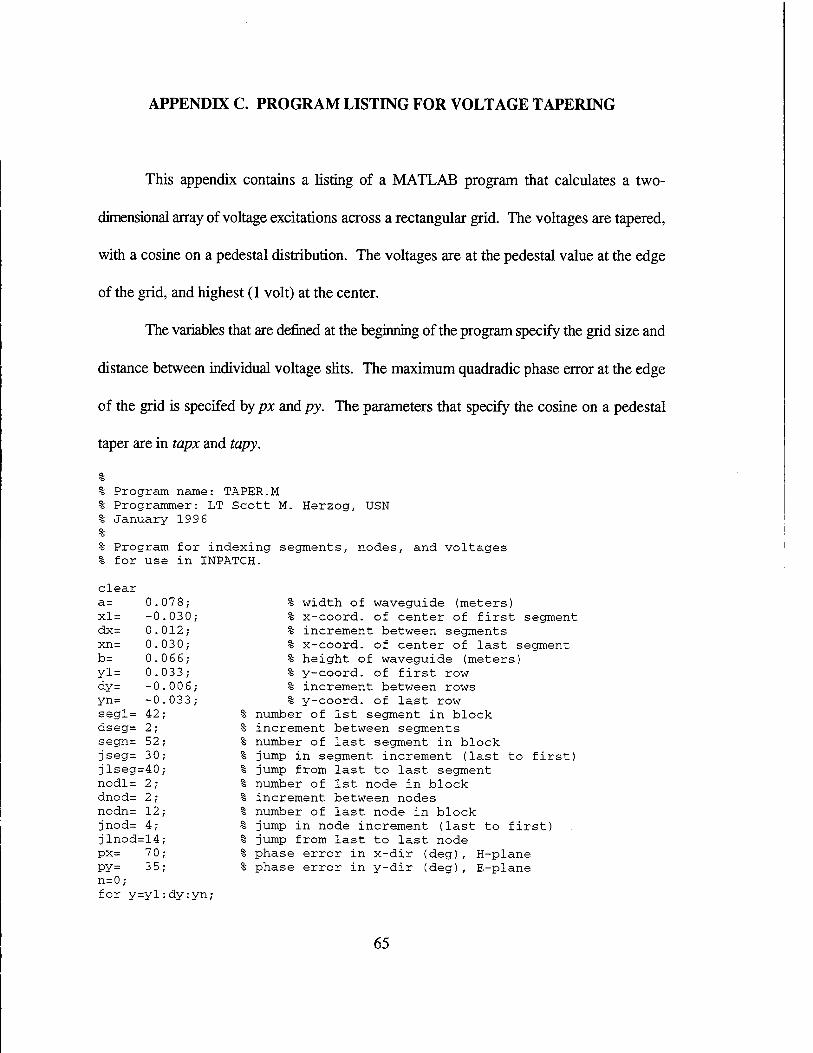
APPENDIX C. PROGRAM LISTING FOR VOLT AGE TAPERING
This appendix contains a listing of a MATLAB program that calculates a two-
dimensional array of voltage excitations across a rectangular grid. The voltages are tapered,
with a cosine on a pedestal distribution. The voltages are at the pedestal value at the edge
of the grid, and highest (1 volt) at the center.
The variables that are defined at the beginning of the program specify the grid size and
distance between individual voltage slits. The maximum quadradic phase error at the edge
of the grid is specifed by px and py. The parameters that specify the cosine on a pedestal
taper are in tapx and tapy.
% % Program name: TAPER.M % Programmer: LT Scott M. Herzog, USN % January 1996 % % Program for indexing segments, nodes, and voltages % for use in INPATCH.
clear a= 0.078; x1= -0.030; dx= 0.012; xn= 0.030; b= 0.066; y1= 0.033; dy= -0.006; yn= -0.033; seg1= 42; dseg= 2; segn= 52; jseg= 30; jlseg=40; nod1= 2; dnod= 2; nodn= 12; jnod= 4; jlnod=14; PX= 70; PY= 35; n=O; for y=y1:dy:yn;
% width of waveguide (meters) % x-coord. of center of first segment % increment between segments % x-coord. of center of last segment % height of waveguide (meters) % y-coord. of first row % increment between rows % y-coord. of last row
% number of 1st segment in block % increment between segments % number of last segment in block % jump in segment increment (last to first) % jump from last to last segment % number of 1st node in block % increment between nodes % number of last node in block % jump in node increment (last to first) % jump from last to last node %phase error in x-dir (deg), H-plane %phase error in y-dir (deg), E-plane
65

end n=O;
for x=xl:dx:xn;
end
n=n+l; phx=exp(j*px*pi/180*(2*x/a)A2); phy=exp(j*py*pi/180*(2*y/b)A2); tapx=(0.1+0.9*cos(pi*x/a)); % H-plane taper tapy=(0.6+0.4*cos(pi*y/b)); % E-plane taper v=tapx*tapy*phx*phy; volt(n)=v;
for y=yl:dy:yn;
end n=O;
for seg=segl:dseg:segn; n=n+l; segrnent(n)=seg;
end segl=segn+jseg; segn=segn+jlseg;
for y=yl:dy:yn;
end
for nod=nodl:dnod:nodn; n=n+l; node(n)=nod;
end nodl=nodn+jnod; nodn=nodn+jlnod;
data=[segment' node' real(volt)' imag(volt) ']; save volt n data -ascii
66

APPENDIX D. PROGRAM LISTING FOR GEOMETRY COMBINING
This appendix contains a listing of a MATLAB program to combine two separate
elements of geometry, such as an aperture and a radome. If the aperture geometry was
created separately from the radome geometry, each file's nodes and edges are numbered
independently, starting with the number one. A geometry file cannot be appended to another,
until the second file's nodes and edges are renumbered. This program renumbers the nodes
and edges of the second geometry file, appends it to the frrst, and saves the combined file
under the name duo.
% Program name: % Programmer: % April 1996 %
COMBINE.M LT Scott M. Herzog, USN
% Combines two independent ASCII data files from the output of % BUILDN5.X. % % Re-indexes the node and edge numbers of the second data file % and appends it to the first. % % Notes on usage: % % (1) Delete comment line in both input files. % (2) Rename first input file FILE1.TXT, typically the aperture. % (3) Rename second input file FILE2.TXT, typically the radome. % (4) Output file saved as DUO, without a comment line. % This must be added!
clear id1 file1= id2 file2=
nodes1 edges1 nodes2 edges2
an1 zn1 ae1 ze1 an2
f open ( 1 f i 1 e 1 . txt 1 ,
1 rt 1 ) ;
fscanf(id1, 1 %e 1);
fopen ( 1 file2. txt 1, I rt 1
) ;
fscanf(id2, 1 %e 1);
file1(1,1); file1 (2,1); file2 (1,1); file2 ( 2, 1) ;
3 i % row no. of nodes1*4+2; % II
zn1+1; % row no. of zn1+edges1*3; % 3 i
% read in first file.
% read in second file.
first element in node block in filel. last first element in edge block in file1. II last
67

zn2 nodes2*4+2; ae2 zn2+1; ze2 zn2+edges2*3;
comb=[nodesl+nodes2 edgesl+edges2];
Nl=reshape(filel(anl:znl 1 l) 1 4 1 nodesl); Nl=Nl'; El=reshape(filel(ael:zel 1 l) 1 3 1 edgesl); El=El'; N2=reshape(file2(an2:zn2 1 l) 1 4 1 nodes2); N2=N2 I;
Nl (: 1 4) Nl ( : I 4) + 0 . 0 7 6 9 9 ;
N2 ( : I 4) N2 (: I 4) - 0 .1452; %N2 ( : I 2 : 4) = 0. 0 01 *N2 ( : I 2 : 4) ; %N2(: 1 2:4) = 0.0254*N2(: 1 2:4); %N2(: 1 2:4) = 0.0205*N2(: 1 2:4); N2(: 1 2:4) = 0.0282369*N2(: 1 2:4);
%
% % % % %
E2=reshape(file2(ae2:ze2 1 l) 1 3 1 edges2); E2=E2 I;
% construct node block matrix
% construct edge block matrix
translate aperture forward.
subtract offset in Z-axis. rescale from rnrn to m. rescale from in to m. rescale from 'units' to m. rescale to ml for some files.
N2(: 1 l)=N2(: 1 l)+nodesl; E2(: 1 l)=E2(: 1 l)+edgesl; E2(: 1 2:3)=E2(: 1 2:3)+nodesl;
% changes node numbers in second file. % changes edge numbers in second file.
save duo comb Nl N2 El E2 -ascii
68

LIST OF REFERENCES
1. Jenn, D. C., Radar and Laser Cross Sectional Engineering, AIAA Education Series, June 19, 1995.
2. Francis, R. M., "A Computer Model for the Transmission Characteristics of Dielectric Radomes," Master's Thesis, Naval Postgraduate School, Monterey, California, March 1992.
3. Klopp, K. A., "Antenna Gain Loss and Pattern Degradation due to Transmission Through Dielectric Radomes," Master's Thesis, Naval Postgraduate School, Monterey, California, March 1993.
4. Johnson, W. A., Wilton, D. R., and Sharpe, R. M., Patch Code Users' Manual, Sandia Report SAND87-2991, May 1988.
5. Sadiku, M. N. 0., Elements of Electromagnetics, second edition, Saunders College Publishing, 1994, p. 466.
6. Chang, D. C., "A Comparison of Computed and Measured Transmission Data for the AGM-88 HARM Radome," Master's Thesis, Naval Postgraduate School; Monterey, California, September 1993.
7. Jenn, D. C., Francis, R. M., and Klopp, K. A., "Computer Model for Axially Symmetric Dielectric Radomes in the Near Field of a Circlular Aperture," unpublished notes, Naval Postgraduate School, Monterey, California.
8. Stutzman, W. L. and Thiele, G. A., Antenna Theory and Design, John Wiley & Sons, Inc., 1981, pp. 184-189.
9. Balanis, C. A., Antenna Theory Analysis and Design, John Wiley and Sons, Inc., 1982, pp. 587-589.
10. Hoppus, G. W., Radio Frequency Guidance Head, NA WCWPNS, China Lake, California, telephone conversation, May 1996.
69

70
![COUNTERMEASURES AGAINST ANTI-RADIATION MISSILES S% … · 2011. 5. 14. · principle of investigating ARM [anti-radiation missile] with coherent or noncoherent dual-sources (quasi-dual-source).](https://static.fdocuments.us/doc/165x107/60655164019a2616922831f9/countermeasures-against-anti-radiation-missiles-s-2011-5-14-principle-of-investigating.jpg)