Radar Doppler Frequency Measurements—Accuracy Versus SNR ...
12
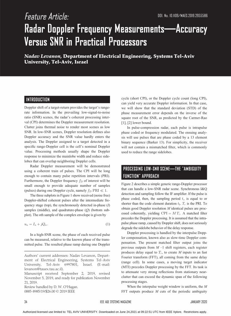
Feature Article: DOI. No. 10.1109/MAES.2019.2955586 Radar Doppler Frequency Measurements —Accuracy Versus SNR in Practical Processors Nadav Levanon, Department of Electrical Engineering, Systems Tel-Aviv University, Tel-Aviv, Israel INTRODUCTION Doppler shift of a target-return provides the target’s range- rate information. In the prevailing low-signal-to-noise ratio (SNR) scenes, the radar’s coherent processing inter- val (CPI) determines the Doppler measurement resolution. Clutter joins thermal noise to render most scenes as low SNR. In low-SNR scenes, Doppler resolution defines also Doppler accuracy and the SNR value hardly enters the analysis. The Doppler assigned to a target detected in a specific range-Doppler cell is the cell’s nominal Doppler value. Processing methods usually shape the Doppler response to minimize the mainlobe width and reduce side- lobes that can overlap neighboring Doppler cells. Radar Doppler measurement will be demonstrated using a coherent train of pulses. The CPI will be long enough to contain many pulse repetition intervals (PRI). Furthermore, the Doppler frequency f D of interest will be small enough to provide adequate number of samples (pulses) during one Doppler cycle, namely f D PRI 1. The three subplots in Figure 1 show received (noise free) Doppler-shifted coherent pulses after the intermediate fre- quency stage (top), the synchronously detected in-phase (I) samples (middle), and quadrature-phase (Q) (bottom sub- plot). The nth sample of the complex envelope is given by u n ¼ I n þ jQ n : (1) In a high-SNR scene, the phase of each received pulse can be measured, relative to the known phase of the trans- mitted pulse. The resulted phase ramp during one Doppler cycle (short CPI), or the Doppler cycle count (long CPI), can yield very accurate Doppler information. In that case, we will show that the standard deviation (STD) of the phase measurement error depends on the inverse of the square root of the SNR, as predicted by the Carmer-Rao [1], [2] lower bound. In pulse-compression radar, each pulse is intrapulse phase coded or frequency modulated. The ensuing analy- sis will use pulses that are phase coded by a 13 element binary sequence (Barker 13). For simplicity, the receiver will not contain a mismatched filter, which is commonly used to reduce the range sidelobes. PROCESSING LOW-SNR SCENE —THE “ AMBIGUITY FUNCTION ” APPROACH Figure 2 describes a simple generic range-Doppler processor that can handle a low-SNR radar scene. Synchronous I&Q detection and sampling follow the IF amplifier. If the pulse is phase coded, then, the sampling period t s is equal to or shorter than the code element duration t b . T r is the PRI. To obtain good Doppler resolution M identical pulses are proc- essed coherently, yielding CPI ¼ MT r . A matched filter precedes the Doppler processing. It is assumed that the intra- pulse phase ramp, caused by Doppler shift, does not seriously degrade the sidelobe behavior of the delay response. Doppler processing is handled by the interpulse Dopp- ler compensation, known also as slow-time Doppler com- pensation. The present matched filter output joins the previous outputs from M –1 shift registers, each register produces delay equal to T r , to create M inputs to an fast Fourier transform (FFT), all coming from the same delay (range cell). In some cases, a moving target indicator (MTI) precedes Doppler processing by the FFT. Its task is to attenuate very strong reflections from stationary near- clutter that can exceed the dynamic span of the following processing stages. When the interpulse weight window is uniform, the M FFT outputs produce M cuts of the periodic ambiguity Authors’ current addresses: Nadav Levanon, Depart- ment of Electrical Engineering, Systems Tel-Aviv University, Tel-Aviv 6997801, Israel. (E-mail: [email protected]). Manuscript received September 2, 2019, revised November 5, 2019, and ready for publication November 21, 2019. Review handled by D. W. O’Hagan. 0885-8985/19/$26.00 ß 2019 IEEE 34 IEEE A&E SYSTEMS MAGAZINE JANUARY 2020 Authorized licensed use limited to: TEL AVIV UNIVERSITY. Downloaded on June 24,2021 at 09:22:51 UTC from IEEE Xplore. Restrictions apply.
Transcript of Radar Doppler Frequency Measurements—Accuracy Versus SNR ...
Feature Article: DOI. No. 10.1109/MAES.2019.2955586
Radar Doppler Frequency Measurements—AccuracyVersus SNR in Practical ProcessorsNadav Levanon,Department of Electrical Engineering, Systems Tel-AvivUniversity, Tel-Aviv, Israel
INTRODUCTION
Doppler shift of a target-return provides the target’s range-
rate information. In the prevailing low-signal-to-noise
ratio (SNR) scenes, the radar’s coherent processing inter-
val (CPI) determines the Doppler measurement resolution.
Clutter joins thermal noise to render most scenes as low
SNR. In low-SNR scenes, Doppler resolution defines also
Doppler accuracy and the SNR value hardly enters the
analysis. The Doppler assigned to a target detected in a
specific range-Doppler cell is the cell’s nominal Doppler
value. Processing methods usually shape the Doppler
response to minimize the mainlobe width and reduce side-
lobes that can overlap neighboring Doppler cells.
Radar Doppler measurement will be demonstrated
using a coherent train of pulses. The CPI will be long
enough to contain many pulse repetition intervals (PRI).
Furthermore, the Doppler frequency fD of interest will be
small enough to provide adequate number of samples
(pulses) during one Doppler cycle, namely fD PRI � 1.
The three subplots in Figure 1 show received (noise free)
Doppler-shifted coherent pulses after the intermediate fre-
quency stage (top), the synchronously detected in-phase (I)
samples (middle), and quadrature-phase (Q) (bottom sub-
plot). The nth sample of the complex envelope is given by
un ¼ In þ jQn: (1)
In a high-SNR scene, the phase of each received pulse
can be measured, relative to the known phase of the trans-
mitted pulse. The resulted phase ramp during one Doppler
cycle (short CPI), or the Doppler cycle count (long CPI),
can yield very accurate Doppler information. In that case,
we will show that the standard deviation (STD) of the
phase measurement error depends on the inverse of the
square root of the SNR, as predicted by the Carmer-Rao
[1], [2] lower bound.
In pulse-compression radar, each pulse is intrapulse
phase coded or frequency modulated. The ensuing analy-
sis will use pulses that are phase coded by a 13 element
binary sequence (Barker 13). For simplicity, the receiver
will not contain a mismatched filter, which is commonly
used to reduce the range sidelobes.
PROCESSING LOW-SNR SCENE—THE “AMBIGUITY
FUNCTION” APPROACH
Figure 2 describes a simple generic range-Doppler processor
that can handle a low-SNR radar scene. Synchronous I&Q
detection and sampling follow the IF amplifier. If the pulse is
phase coded, then, the sampling period ts is equal to or
shorter than the code element duration tb. Tr is the PRI. To
obtain good Doppler resolution M identical pulses are proc-
essed coherently, yielding CPI ¼ M Tr. A matched filter
precedes the Doppler processing. It is assumed that the intra-
pulse phase ramp, caused by Doppler shift, does not seriously
degrade the sidelobe behavior of the delay response.
Doppler processing is handled by the interpulse Dopp-
ler compensation, known also as slow-time Doppler com-
pensation. The present matched filter output joins the
previous outputs from M –1 shift registers, each register
produces delay equal to Tr, to create M inputs to an fast
Fourier transform (FFT), all coming from the same delay
(range cell). In some cases, a moving target indicator
(MTI) precedes Doppler processing by the FFT. Its task is
to attenuate very strong reflections from stationary near-
clutter that can exceed the dynamic span of the following
processing stages.
When the interpulse weight window is uniform, the M
FFT outputs produce M cuts of the periodic ambiguity
Authors’ current addresses: Nadav Levanon, Depart-ment of Electrical Engineering, Systems Tel-AvivUniversity, Tel-Aviv 6997801, Israel. (E-mail:[email protected]).Manuscript received September 2, 2019, revisedNovember 5, 2019, and ready for publication November21, 2019.Review handled by D. W. O’Hagan.0885-8985/19/$26.00 � 2019 IEEE
34 IEEE A&E SYSTEMS MAGAZINE JANUARY 2020
Authorized licensed use limited to: TEL AVIV UNIVERSITY. Downloaded on June 24,2021 at 09:22:51 UTC from IEEE Xplore. Restrictions apply.

function (PAF) [3], [4]. This explains the name given to
this approach. When the pulse duration tp is short relative
to the PRI, namely tp < Tr=2 then the PAF is given by
xM Tr t; nð Þ�� �� ¼ x t; nð Þj j sin MTrpnð ÞM sin Trpnð Þ���� ���� (2)
where x ðt; nÞ is the Woodward’s ambiguity function [4]
of a single pulse, t is delay, and n will represent Doppler
shift (together with fD ). The Doppler resolution is given
by the cut of (2) at zero delay. Setting t ¼ 0 in (2) yields
xM Tr 0; nð Þ�� �� ¼ x 0; nð Þj j sin MTrpnð ÞM sin Trpnð Þ���� ����: (3)
One of the properties of the AF is that its zero-delay
cut is independent of any phase or frequency modulation,
but depends only on the magnitude of the pulse’s complex
envelopeuðtÞ,
x 0; nð Þj j ¼Z tp=2
�tp=2
u tð Þj j2exp j2pntð Þ dt�����
�����: (4)
In our example the pulse is phase coded, but its ampli-
tude is constant, which results in
x 0; nð Þj j ¼ sin tp p n� �tpp n
���� ����: (5)
Inserting (5) in (3) yields the expected Doppler
response of a coherent train of M identical phase coded
(or frequency modulated) pulses,
xMTr0; nð Þ�� �� ¼ sin tp p n
� �tpp n
���� ���� sin MTrpnð ÞMsin Trpnð Þ
���� ����: (6)
Using a decibel scale, Figure 3 displays (6), for the
case of M ¼ 32 ; Tr=tp ¼ 5 ) MTr=tp ¼ 160. For
such a case, the first term on the right-hand side (r.h.s.) of
(6) hardly influences the Doppler response. Its effect is
seen by the attenuation of 0.6 dB of the recurrent lobes at
f MTr ¼ � 32. Note that the Doppler resolution (defined
as the separation between the mainlobe’s peak and the first
null) is Dn ¼ Df ¼ 1=ðM TrÞ ¼ 1=CPI.
Nonuniform weight windows, such as Hamming,
Dolph-Chebyshev, [5], [6] can help reduce the sidelobes
of the Doppler response, with a penalty of wider mainlobe.
To avoid transmitting pulses of different amplitudes, the
weight window appears only at the receiver side, causing
mismatch, hence the SNR loss. Typical loss is about
1.5 dB (e.g., in the Hamming case). Figure 4 displays the
normalized Doppler response when a Hamming window
is used. Note the reduced Doppler sidelobes and the dou-
bling of the Doppler resolution.
Figures 3 and 4 show that the Doppler resolution
achieved by the processor outlined in Figure 2 is either
Dn ¼ 1=ðMTrÞ, without interpulse amplitude weight win-
dow, or Dn ¼ 2=ðMTrÞwhen a Hamming weight window
is used. To learn the two-dimensional range-Doppler
response, we need to define a more specific waveform. To
keep the example simple, we will add Barker 13 binary
phase-coding to the previous example. With this choice,
the duration of a code element is tb ¼ tp=13. We will also
add Doppler shift. Figure 5 displays the noise-free
phase evolution along six (out of 32) received pulses.
From a phase change during one PRI, Df ¼ 0:5893 rad,
we can derive the normalized dimensionless Doppler
shift ntb ¼ 0:5893=ð130pÞ ¼ 0:0014; nTr ¼ 0:0938,
and finally nMTr ¼ 3. The last normalization is the
one used in the delay-Doppler responses shown in
Figures 6 and 7.Figure 1.Coherent I and Q sampling of a Doppler shifted pulse train.
JANUARY 2020 IEEE A&E SYSTEMS MAGAZINE 35
Authorized licensed use limited to: TEL AVIV UNIVERSITY. Downloaded on June 24,2021 at 09:22:51 UTC from IEEE Xplore. Restrictions apply.

Figure 3.Doppler response of an unweighted coherent train of 32 unimodular pulses.
Figure 2.Generic delay-Doppler processor of a coherent train of identical coded pulses.
Figure 4.Normalized Doppler response of a coherent train of 32 pulses, Hamming amplitude weighted on receive.
Radar Doppler Frequency Measurements—Accuracy Versus SNR in Practical Processors
36 IEEE A&E SYSTEMS MAGAZINE JANUARY 2020
Authorized licensed use limited to: TEL AVIV UNIVERSITY. Downloaded on June 24,2021 at 09:22:51 UTC from IEEE Xplore. Restrictions apply.

Figure 6 presents the response when a uniform
weight window is used. As expected, the mainlobe is
located at t ¼ 0; nMTr ¼ 3. The range sidelobes are
the well-known Barker 13 sidelobes with peak sidelobe
level (PSL) of 1=13 ¼ 0:0769. The Doppler sidelobes
match Figure 3. Figure 7 presents the response when a
Hamming weight window is used. The Doppler main-
lobe width doubled and the Doppler sidelobes dropped
to typical peaks of 20log10(0.007952) ¼ –42 dB. While
the matched filter did not compensate the Doppler-
induced intrapulse phase ramp, we see no effect on the
range sidelobes pattern and heights. In case of a longer
Figure 5.Noise-free phase evolution of Doppler shifted 6 (out of 32) received pulses.
Figure 6.Delay-Doppler response of the processor (uniform weight window) to the Doppler shifted waveform.
Figure 7.Delay-Doppler response of the processor (Hamming weight window) to the Doppler shifted waveform.
Levanon
JANUARY 2020 IEEE A&E SYSTEMS MAGAZINE 37
Authorized licensed use limited to: TEL AVIV UNIVERSITY. Downloaded on June 24,2021 at 09:22:51 UTC from IEEE Xplore. Restrictions apply.

code and higher duty cycle, some degradation should be
expected.
Note that Figure 7 displays the normalized response,
in which the peak attains a unit value. Without normaliza-
tion, a loss due to a Hamming window on receive would
have caused a drop of about 1.5 dB in the peak.
With this kind of Doppler processing, the duration of
the CPI determines the Doppler resolution. The first Dopp-
ler null, next the peak at n ¼ 0, will appear at n ¼ 1=CPI.
Using a nonuniform interpulse weight window (e.g., Ham-
ming) will approximately double the Doppler resolution.
A target detected by threshold crossing, at a specific out-
put of the FFT (in the unavoidable presence of noise and
clutter), is assigned the Doppler shift value associated
with that FFT output. Low SNR does not alter the resolu-
tion, but can prevent threshold crossing, causing missed
detection. Figures 8 and 9 show the delay-Doppler
responses of the signal used so far, at SNR values of
–10 dB and –20 dB, respectively.
We should point out that in the processor producing
Figures 8 and 9, the complex envelope of the signal-
plus-noise passed through a low-pass Butterworth filter of
order one and vn ¼ 0:15; and there were ten samples per
code element. Uniform weight window was used; hence,
the noise-free response to compare is the one in Figure 6.
The response in Figure 8 indicates reasonable probability
of detection, while lowering the threshold below the peak
value in Figure 9 is likely to cause high probability of false
alarm. Note that the stated SNR is per sample and before
the filter.
The “Ambiguity Function” Doppler frequency estima-
tion approach, discussed in this section, aims at the pre-
vailing low-SNR radar scene. However, in high-SNR
scenes, it can be modified to produce the frequency
Figure 8.Normalized delay-Doppler response to the Doppler shifted waveform, SNR ¼ –10 dB,M ¼ 32.
Figure 9.Normalized delay-Doppler response to the Doppler shifted waveform, SNR ¼ –20 dB,M ¼ 32.
Radar Doppler Frequency Measurements—Accuracy Versus SNR in Practical Processors
38 IEEE A&E SYSTEMS MAGAZINE JANUARY 2020
Authorized licensed use limited to: TEL AVIV UNIVERSITY. Downloaded on June 24,2021 at 09:22:51 UTC from IEEE Xplore. Restrictions apply.

estimation with better accuracy than the resolution
Dn ¼ Df ¼ 1=ðMTrÞ ¼ 1=CPI. In a high-SNR scene,
zero-padding the FFT can be used. Furthermore, if the
exact Doppler frequency is located between two nominal
frequencies, corresponding to two neighboring FFT out-
puts, the estimated frequency need not be the nominal fre-
quency of the FFT cell whose output is the highest.
Interpolation can be used to estimate a more exact location
of the spectrum peak. A qualitative example is demon-
strated in Figures 10 (noise-free) and 11 (SNR ¼ –2 dB,
per sample).
In the noise-free case (see Figure 10), interpolating the
lower subplot would have correctly placed the spectral
peak to the left of the 9.375 Hz cell. In the low-SNR case
(see Figure 11), interpolation would have erroneously
placed the peak at about half way between 9.375 and the
12.5 Hz cells.
PROCESSING HIGH-SNR SCENES
In rare radar scenes, where the signal-to-clutter plus
noise ratios are high, the concept of Doppler measure-
ment accuracy (or precision) becomes relevant, includ-
ing its dependence on SNR. By accuracy, we refer to
the noise-induced error standard deviation. Mean
error, usually caused by other error sources, will be
ignored [7].
Returning to the Doppler shifted, noise-free, phase
evolution in Figure 5, our ad-hoc Doppler measuring con-
cept will be based on measuring the phase of each pulse
(after compression). Assuming no change of the target’s
range rate during the CPI, the Doppler frequency will be
derived from the slope of the unwrapped line connecting
the measured phases.
PHASE MEASUREMENT
The phase of a single compressed pulse will be determined
by tan�1ðQp=IpÞ, where Qp; IP are the quadrature and in-
phase values of the sample corresponding to the peak of
the matched filter response (i.e., the correlation of the
received coded pulse and the noise-free coded reference).
In high-SNR scenes finding the closest sample to the peak
is rather simple if there are enough samples per code
elements.
Figure 12 (top) shows the complex envelope of the
Barker 13 signal used in the phase measurement example.
xs is the pre LPF waveform and ys is the post LPF wave-
form. Note that the complex envelope is real, having no
Figure 10.(Top) True spectrum, after LPF, of an 8.2-Hz single tone; (Bottom) FFT outputs of 16 samples. Noise free case.
Figure 11.(Top) Spectrum after LPF, of a noisy 8.2-Hz single tone; (Bottom) FFT outputs of the 16 samples. SNR ¼ –2 dB per sample.
Levanon
JANUARY 2020 IEEE A&E SYSTEMS MAGAZINE 39
Authorized licensed use limited to: TEL AVIV UNIVERSITY. Downloaded on June 24,2021 at 09:22:51 UTC from IEEE Xplore. Restrictions apply.

imaginary component. This fact implies that the reference
signal’s phase is zero. The red solid lines in the middle
and bottom subplots show the real and imaginary values
after complex random noise is added to the low-pass fil-
tered Barker 13. This is a low-SNR case, in which SNR ¼–7dB. Note that there are ten samples per coding bit dura-
tion tb. Note also that the stated SNR is per sample and
before the filter.
The receiving processor performs cross correlation
between the noise-free reference signal ys and the noisy
signal ysþyn. Figure 13 displays the magnitude (top) and
phase (bottom) of the cross correlation. The display zooms
on ten coding bits, namely, the delay span is
�10 � t=tb � 10. At this SNR level, the correlation
magnitude peak is still well defined above the sidelobes,
allowing simple determination of the target’s delay. One
possible technique is to use convolution with a split-gate
[8], and to find the zero-crossing point of the convolution
output. A simpler technique is to choose the mid delay
sample between two threshold crossings: at the rise and
fall of the convolution mainlobe. The phase value (bottom
plot) shows the expected zero phase value around the
delays corresponding to the peak of the correlation’s
magnitude.
Monte Carlo simulation, repeated 5000 times at each
SNR value, produced the phase measurement error STD
as function of SNR as presented in Figure 14. A line
(dash, red) representing fSTD ¼ 2:095=ffiffiffiffiffiffiffiffiffiffiSNR
pwas fitted
Figure 12.Noise-free waveform before and after LPF (top). The real part of the received signal þ noise (middle) and the imaginary part (bottom).
SNR ¼ –7dB.
Figure 13.Magnitude (top) and phase (bottom) of the cross-correlation output.
Radar Doppler Frequency Measurements—Accuracy Versus SNR in Practical Processors
40 IEEE A&E SYSTEMS MAGAZINE JANUARY 2020
Authorized licensed use limited to: TEL AVIV UNIVERSITY. Downloaded on June 24,2021 at 09:22:51 UTC from IEEE Xplore. Restrictions apply.

to the �10 � SNR � 5 dB span of the curve to demon-
strate the expected error dependence on SNR�1=2.
The phase error curve demonstrates the three typical
zones of error versus SNR. In the high-SNR zone (on the
right), the phase error follows a SNR�1=2 law. In the left
zone, at very low SNRs, the error curve is flat aroundffiffiffiffiffiffiffiffiffiffiffiffiffiffivarðfÞp � 103�, as seen in the left-most data tip. It is
known as the no information zone and the error level as
the a priori bound. When the SNR is very low, the mea-
sured phase is uniformly distributed over all possible
phase values, yielding
var fð Þ ¼ 1
360
Z 180
�180
f2df
¼ 1
180
Z 180
0
f2df ¼ 1
180
f3
3
� �1800
¼ 1802
3)
ffiffiffiffiffiffiffiffiffiffiffiffiffiffivar fð Þ
p¼ 180ffiffiffi
3p ¼ 103:9�:
(7)
The two SNR zones are connected by the transition
zone, in which the phase error increases rapidly as the SNR
drops. Using a longer coding sequence will allow accurate
measurements at lower SNR values. With a 48 element
Minimum Peak Side Lobe code, the high-SNR zone of the
curve will shift left by 10log10ð48=13Þ ¼ 5:67 dB.
FROM PHASE MEASUREMENT TO FREQUENCY
MEASUREMENT
Frequency cannot be measured instantly. Accurate esti-
mate of the Doppler frequency can be derived from the set
of measurements of the phase of each received pulse in
the coherent train (e.g., the 32 pulses used in the section
“Processing Low SNR Scene—The “Ambiguity Function”
Approach). The known PRI of the transmitted pulses can
ease finding the expected location of the correlation peak,
from where the phase value of each pulse is extracted.
The assumption that the target’s range rate does not
change during the CPI implies that the noise-free phase
measurement should be a linear function of time. The
slope of the line is the angular frequency v of the Doppler
shift,
f tmð Þ ¼ f0 þ vtm þ ym; tm ¼ mTr;
m ¼ 0; 1; . . . ;M � 1(8)
where Tr is the PRI and ym is the error of the measured
phase of the mth pulse.
We will also assume that the phase measurements
errors are uncorrelated and have identical variance s2f so
that the phase errors covariance matrix is
Rf ¼ s2f I (9)
where I is an identity matrix of size M. We will use linear
least square (LS) to estimate the two line parameters,
defined by the parameters vector
x ¼ f0 v½ �T (10)
from the M phase measurements, defined by the measure-
ments vector
f ¼ f1 f1 . . .fm . . .fM½ �T : (11)
Figure 14.Phase error STD as function of SNR, obtained from Monte Carlo simulation.
Levanon
JANUARY 2020 IEEE A&E SYSTEMS MAGAZINE 41
Authorized licensed use limited to: TEL AVIV UNIVERSITY. Downloaded on June 24,2021 at 09:22:51 UTC from IEEE Xplore. Restrictions apply.
We will also arrange the phase measurements errors in
an errors vector
yy ¼ y1 y1 . . . ym . . . yM½ �T : (12)
Finally, we define the (M x 2) matrix H that will allow
us to describe theM equations in (8) as theM-dimensional
measurements vector in (11)
H ¼ 1 1 1 . . . 1 . . . 10 Tr 2Tr . . . mTr . . . M � 1ð ÞTr
� �T: (13)
The resulted matrix equation is
f ¼ Hxþ yy:: (14)
The well-known [9] LS solution of the parameters
vector is
x̂LS ¼ HTH� ��1
HTf: (15)
Well known also is the covariance of the errors of the
estimated parameters
P ¼ E x̂LSx̂TLS
� ¼ s2f HTH� ��1
: (16)
Inserting (13) in (16) yields
P ¼ s2f HTH� ��1 ¼ s2
f
12
M4 �M2
16M M � 1ð Þ 2M � 1ð Þ �1
2 M M � 1ð Þ=Tr
�12 M M � 1ð Þ=Tr M=T 2
r
" #:(17)
The error variance of the angular Doppler frequency v
is P2,2, hence
s2v ¼ 12
MTrð Þ2 M � 1=Mð Þ s2f: (18)
We will convert (18) to Doppler frequency
f ¼ v=ð2pÞ, perform square root and normalize the fre-
quency to create a dimensionless variable by multiplying
the frequency by the CPI, i.e., byMTr,
MTrsf ¼ sf
p
ffiffiffiffiffiffiffiffiffiffiffiffiffiffiffiffiffiffiffiffiffi3
M � 1=M
s: (19)
The important expression in (19) says that the SNR
dependence of the normalized frequency error MTrsf is
shaped like the SNR dependence of the phase error, multi-
plied by an expression that is a function of M. Using the
data from Figure 14, we can construct a short table
expressing that dependence.
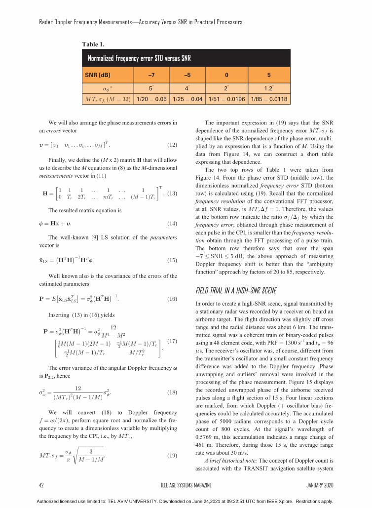
The two top rows of Table 1 were taken from
Figure 14. From the phase error STD (middle row), the
dimensionless normalized frequency error STD (bottom
row) is calculated using (19). Recall that the normalized
frequency resolution of the conventional FFT processor,
at all SNR values, is MTrDf ¼ 1. Therefore, the values
at the bottom row indicate the ratio sf=Df by which the
frequency error, obtained through phase measurement of
each pulse in the CPI, is smaller than the frequency resolu-
tion obtain through the FFT processing of a pulse train.
The bottom row therefore says that over the span
�7 � SNR � 5 dB, the above approach of measuring
Doppler frequency shift is better than the “ambiguity
function” approach by factors of 20 to 85, respectively.
FIELD TRIAL IN A HIGH-SNR SCENE
In order to create a high-SNR scene, signal transmitted by
a stationary radar was recorded by a receiver on board an
airborne target. The flight direction was slightly off cross
range and the radial distance was about 6 km. The trans-
mitted signal was a coherent train of binary-coded pulses
using a 48 element code, with PRF ¼ 1300 s-1 and tp ¼ 96
ms. The receiver’s oscillator was, of course, different from
the transmitter’s oscillator and a small constant frequency
difference was added to the Doppler frequency. Phase
unwrapping and outliers’ removal were involved in the
processing of the phase measurement. Figure 15 displays
the recorded unwrapped phase of the airborne received
pulses along a flight section of 15 s. Four linear sections
are marked, from which Doppler (þ oscillator bias) fre-
quencies could be calculated accurately. The accumulated
phase of 5000 radians corresponds to a Doppler cycle
count of 800 cycles. At the signal’s wavelength of
0.5769 m, this accumulation indicates a range change of
461 m. Therefore, during those 15 s, the average range
rate was about 30 m/s.
A brief historical note: The concept of Doppler count is
associated with the TRANSIT navigation satellite system
Table 1.
Normalized Frequency error STD versus SNR
SNR [dB] –7 –5 0 5
sf� 5
�4
�2
�1.2
�
M Tr sf; ðM ¼ 32Þ 1/20 ¼ 0.05 1/25 ¼ 0.04 1/51 ¼ 0.0196 1/85¼ 0.0118
Radar Doppler Frequency Measurements—Accuracy Versus SNR in Practical Processors
42 IEEE A&E SYSTEMS MAGAZINE JANUARY 2020
Authorized licensed use limited to: TEL AVIV UNIVERSITY. Downloaded on June 24,2021 at 09:22:51 UTC from IEEE Xplore. Restrictions apply.

[10]. The concept and its implementation in TRANSIT navi-
gation receivers are clearly described in [11].
PULSE-PAIR DOPPLER PROCESSING
Another high-SNR approach finds application in weather
radars [12, 7(Ch. 5)]. A rain cloud usually occupies more
than one spatial cell and a given cell contains an extended
target with a relatively wide Doppler spectral width. The
parameters of interest are reflection intensity, average
Doppler frequency, and the Doppler spectral width. We
will consider only the average Doppler frequency, which
is easily obtained from the first leg of the Doppler signal’s
autocorrelation [12].
Doppler signal synchronously detected from a single
moving scatterer will be a single-tone sinewave at a fre-
quency fD, sampled at a rate equal to the radar PRF.
Within the duration of CPI ¼ MTr, the sampled sinewave
is given by
y m½ � ¼ Aej2pfDmTr ; m ¼ 0; . . . ;M � 1: (20)
The first coefficient of the signal’s autocorrelation is
given by
Ry 1½ � XM�2
m¼0
y m½ �y mþ 1½ �: (21)
Using (20) in (21) yields
Ry 1½ � ¼XM�2
m¼0
Aej2pfDmTrAe�j2pfD mþ1ð ÞTr
¼ Aj j2XM�2
m¼0
e�j2pfDTr ¼ Aj j2e�j2pfDTrXM�2
m¼0
1ð Þ
;Ry 1½ � ¼ Aj j2 M � 1ð Þe�j2pfDTr :
(22)
The Doppler frequency appears in the argument of the
first leg of the signal’s autocorrelation
arg Ry 1½ � � ¼ �2pfDTr: (23)
Hence, the estimated Doppler frequency is given by
f̂D ¼ �1
2pTrarg Ry 1½ � �
: (24)
An example of pulse-pair processing is demonstrated
by a real signal constructed from two close sinewaves of
equal amplitude and carriers at f1 ¼ 7.6 Hz and f2 ¼ 8.2
Hz. The detailed expression is
s tð Þ ¼ Re exp j2pf1tð Þ þ exp j 2pf2t� 4p=7ð Þ½ �f g: (25)
The signal and its power spectrum are shown in
Figure 16.
In a noise-free case and two sinewaves of the same
amplitude, the estimated Doppler frequency was exactly
at the middle frequency 7.9 Hz. In the presence of noise,
the random frequency error will be a function of the SNR
and the number M of pulses within the CPI. As can be
deduced from (21), the lower limit is M ¼ 2 pulses. This
Figure 15.Recorded phases of about 20000 coherent radar pulses received
by an airborne receiver.
Figure 16.Two sinewave signals (top) and their spectrum (bottom).
Levanon
JANUARY 2020 IEEE A&E SYSTEMS MAGAZINE 43
Authorized licensed use limited to: TEL AVIV UNIVERSITY. Downloaded on June 24,2021 at 09:22:51 UTC from IEEE Xplore. Restrictions apply.

explains the name “pulse-pair.” The “pulse-pair” approach
can be used also to measure the Doppler shift of a radar
return from a small target, rather than a rain cloud. In that
case, the detected Doppler signal is a noisy sine wave.
The dependence on SNR of the frequency measurement
error of M samples of a single frequency sinewave, using
the “pulse-pair” approach, is described next.
Monte Carlo simulations (see Figure 17) were per-
formed for estimating the frequency of a single sinewave
at 8.2 Hz with a noise span of �15 dB � SNR � 15 dB.
The simulations reveal that the frequency error STD,
obtained by the “pulse-pair” method at high SNR, is pro-
portional to the inverse of the SNR, rather than to the
inverse offfiffiffiffiffiffiffiffiffiffiSNR
p, as was the case in the section “From
Phase Measurement to Frequency Measurement.” The
other parameters of the simulation were Tr ¼ 0.01 s and
M ¼ 1000, yielding CPI ¼ MTr ¼ 10 s. At a Doppler
frequency of 8.2 Hz, the CPI contained 82 cycles. The
Monte Carlo simulations reveal dependence of the error of
the measured normalized frequency Tr sf on both SNR
and the number M of samples (¼ pulses) within the CPI,
according to the expression
Trs bfD
� a TrM
�1=2=SNR: (26)
The dependence of error STD on SNR-1 (rather than
on SNR-1/2) is revealed by the identical slope of the dotted
red line and the simulation result. The dependence on M-1/
2 is learned from the fact that the dotted red line will
remain aligned with the Monte Carlo result despite
changes in the parameter M. The error dependence on
SNR-1 can be seen also in (2.11) in [12], when setting the
spectrum width (w) to zero. The additional dependence on
M is also in agreement with [12]. In Figure 17, a priori
bound in the no-information SNR zone states what is the
STD of the frequency measurement when there is no sig-
nal, just random noise. It is therefore determined mostly
by the frequency response of the filter used. In Figure 17
the high-SNR zone begins at about SNR ¼ 2 dB, where
the normalized error is
Trsf ¼ 0:0013 ) sf ¼Tr¼0:01
0:13 Hz: (27)
Namely, at an SNR ¼ 2 dB and CPI ¼ 10 s, the nomi-
nal frequency of 8.2 Hz is measured with an error STD of
0.13 Hz. Example of the signal þ noise, with SNR (before
LPF) of 2 dB is shown in Figure 18. The plot contains 2 s
out of a CPI of 10 s.
CONCLUSION
The accuracy of frequency measurement in radar and its
dependence on SNR was demonstrated using three
approaches: (a) The classical Pulse-Doppler processor
that performs FFT on the same-delay returns fromM conse-
cutive pulses. We labeled it as the “ambiguity function”
approach. (b) The “Doppler count” approach, in which the
phase of each returning pulse is measured and the Doppler
frequency is estimated from the slope of the phase ramp,
Figure 17.Frequency error STD versus SNR, using the pulse-pair approach,
MTr ¼ 10 s,M ¼ 1000.
Figure 18.2 s of 8.2-Hz sinewave: noise-free (top), SNR ¼ 2 dB (middle), after LPF (bottom).
Radar Doppler Frequency Measurements—Accuracy Versus SNR in Practical Processors
44 IEEE A&E SYSTEMS MAGAZINE JANUARY 2020
Authorized licensed use limited to: TEL AVIV UNIVERSITY. Downloaded on June 24,2021 at 09:22:51 UTC from IEEE Xplore. Restrictions apply.

after unwrapping. (c) The “pulse-pair” approach, devel-
oped for early weather radars, in which the center fre-
quency of the Doppler shift spectrum is calculated from the
first leg of the signal’s autocorrelation. The error attained
in approach (a) is SNR independent, down to an SNR level
belowwhich detection fails. At high-SNR scenes, approach
(b) demonstrates error STD dependence on SNR-1/2, which
is a classical estimation behavior at high SNR. In approach
(c), our simulations confirm and demonstrate a frequency
error STD dependence on SNR-1, which is rather poor
compared to approach (b), but simpler to implement.
REFERENCES
[1] C. E. Cook and M. Bernfeld, Radar Signals an Introduc-
tion to Theory and Applications. New York, NY, USA:
Academic, 1967, ch. 5.
[2] H. L. Van Tress, Detection, Estimation, and Modulation
Theory, Part III. New York, NY, USA: Wiley, 1971, sec.
10.2.
[3] N. Levanon and E. Mozeson, Radar Signals. New York,
NY, USA: Wiley, 2004, sec.3.6.
[4] N. Levanon, “The periodic ambiguity function—Its valid-
ity and value,” in Proc. IEEE Int. Radar Conf., Washing-
ton, DC, USA, 2010, pp. 204–208.
[5] F. J. Harris, “On the use of windows for harmonic analysis
with the discrete Fourier transform,” Proc. IEEE, vol. 69,
no. 1, pp. 51–83, Jan. 1978.
[6] K. M. M. Prabhu, Window Functions and Their Applica-
tions in Signal Processing. Boca Raton, FL, USA: CRC
Press, 2018.
[7] M. A. Richards, Fundamentals of Radar Signal Process-
ing, 2nd ed. New York, NY, USA: McGraw-Hill, 2014,
ch. 7.
[8] D. K. Barton and H. R. Ward, Handbook of Radar Mea-
surement. Dedham, MA, USA: Artech House, sec. 3.5.
[9] H. W. Sorenson, Parameter Estimation: Principles and
Problems. New York, NY, USA: Marcel Dekker, 1980.
[10] W. H. Guier and G. C Weiffenbach, “A satellite
Doppler navigation system,” Proc. IRE, vol. 48, no. 4,
pp. 507–516, Apr. 1960.
[11] T. A. Stansell, “The TRANSIT navigation satellite
system,” Magnavox Rep. R-5933A, Jun. 1983.
[Online]. Available https://www.ion.org/museum/files/
TransitBooklet.pdf Accessed on: Jul. 24, 2019.
[12] F. C. Brenham, H. L. Groginsky, A. S. Soltes, and
G. A Works, “Pulse pair estimation of Doppler spectrum
parameters,” Raytheon Rep., AFCRL-72-0222, Mar. 30,
1972. [Online]. Available: https://apps.dtic.mil/dtic/tr/
fulltext/u2/744094.pdf, Accessed on: Jul. 24, 2019.
Levanon
JANUARY 2020 IEEE A&E SYSTEMS MAGAZINE 45
Authorized licensed use limited to: TEL AVIV UNIVERSITY. Downloaded on June 24,2021 at 09:22:51 UTC from IEEE Xplore. Restrictions apply.