3.0 DETECTION THEORY

3.1 INTRODUCTION

In some of our radar range equation problems we looked at finding the detection range based on SNRs of 13 and 20 dB. We now want to develop some of the theory that explains the use of these particular SNR values. More specifically, we want to examine

the concept of detection probability, . Our need to study detection from a probabilistic perspective stems from the fact that the signals we deal with are noise-like. From our studies of RCS we found that, in practice, the signal return looks random. In fact, Swerling has convinced us that we should use statistical models to represent target signals. Also, in addition to the target signal we found that the signals in the radar contain a noise component, which also needs to be dealt with using the concepts of random variables, random processes and probabilities.

To develop the requisite equations for detection probability we need to develop a mathematical characterization of the target signal, the noise signal and the target-plus-noise signal at various points in the radar. From the above, we will use the concepts of random variables and random processes to characterize these quantities. We start with a characterization of noise and then progress to the target and target-plus-noise signals.

3.2 NOISE IN RECEIVERS

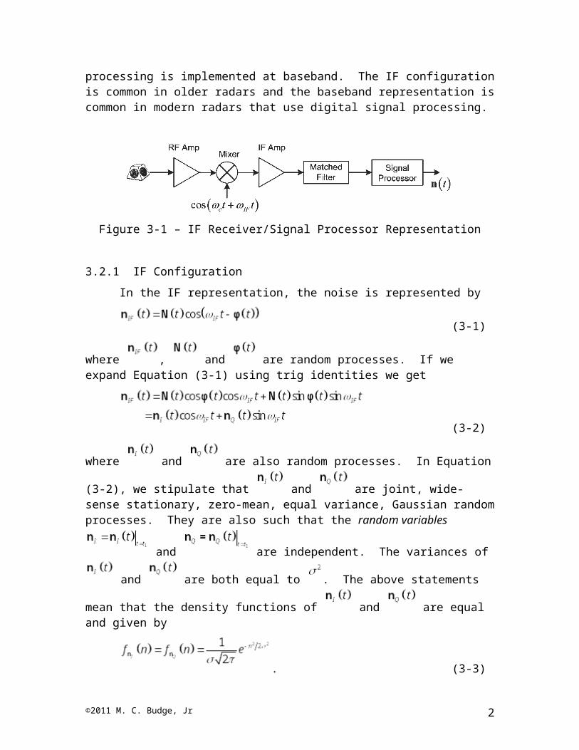
We will characterize noise for the two most common types of receiver implementations. The first receiver configuration is illustrated in Figure 3-1 and is termed the IF representation. In this representation, both the matched filter and the signal processor are implemented at some intermediate frequency, or IF. The second receiver configuration is illustrated in Figure 3-2 and is termed the baseband representation. In this configuration, the signal processing is implemented at baseband. The IF configuration is common in older radars and the baseband representation is common in modern radars that use digital signal processing.

Figure 3-1 – IF Receiver/Signal Processor Representation

3.2.1 IF Configuration

In the IF representation, the noise is represented by

©2011 M. C. Budge, Jr 1

(3-1)

where , and are random processes. If we expand Equation (3-1) using trig identities we get

(3-2)

where and are also random processes. In Equation (3-2), we stipulate that

and are joint, wide-sense stationary, zero-mean, equal variance, Gaussian

random processes. They are also such that the random variables and

are independent. The variances of and are both equal to .

The above statements mean that the density functions of and are equal and given by

. (3-3)

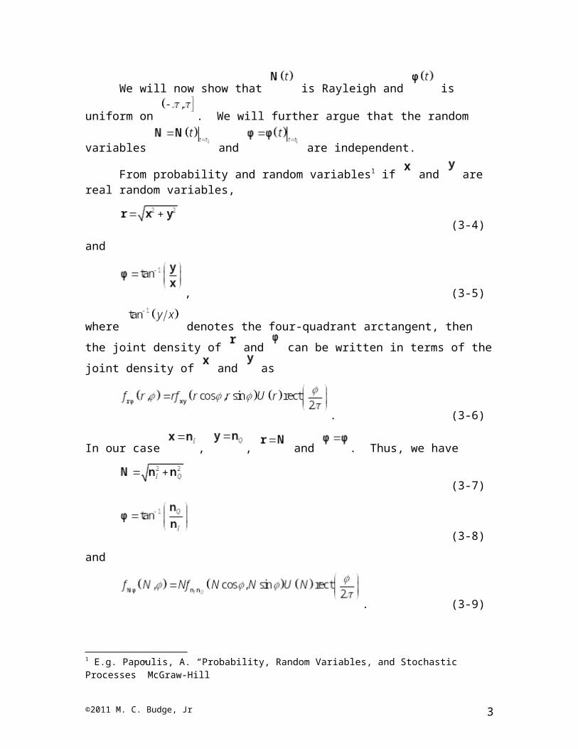
We will now show that is Rayleigh and is uniform on . We

will further argue that the random variables and are independent.

From probability and random variables1 if and are real random variables,

(3-4)

and

, (3-5)

where denotes the four-quadrant arctangent, then the joint density of and

can be written in terms of the joint density of and as

1 E.g. Papoulis, A. “Probability, Random Variables, and Stochastic Processes” McGraw-Hill

©2011 M. C. Budge, Jr 2

. (3-6)

In our case , , and . Thus, we have

(3-7)

(3-8)

and

. (3-9)

Now, since and are independent, Gaussian and zero-mean with equal variance

. (3-10)

If we use this in Equation (3-9) with and we get

. (3-11)

From random variable theory, we can find the marginal density from the joint density by integrating with respect to the variable we want to eliminate. Thus,

(3-12)

and

. (3-13)

©2011 M. C. Budge, Jr 3

This proves the assertion that is Rayleigh and is uniform on . To

prove that the random variables and are independent we note from Equations (3-11), (3-12) and (3-13) that

, (3-14)

which means that and are independent.

Since we will need it later, we want to find the noise power out of the signal

processor. Since is wide-sense stationary we can use Equation (3-2) and write

(3-15)

In Equation (3-15), the term on the third line is zero because and

are independent and zero-mean.

3.2.2 Baseband Configuration

Figure 3-2 – Baseband Receiver/Signal Processor Representation

In the baseband configuration of Figure 3-2 we represent the noise at the signal processor output as a complex random process of the form

©2011 M. C. Budge, Jr 4

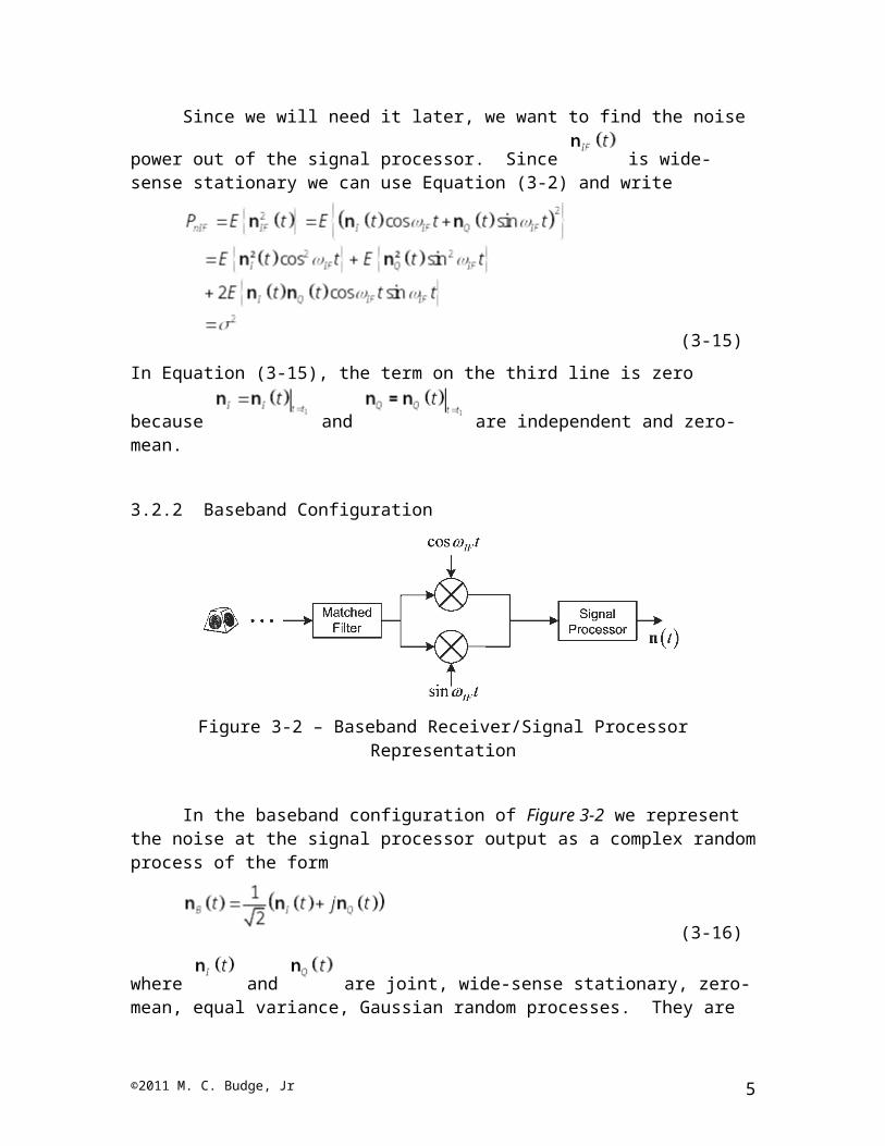
(3-16)

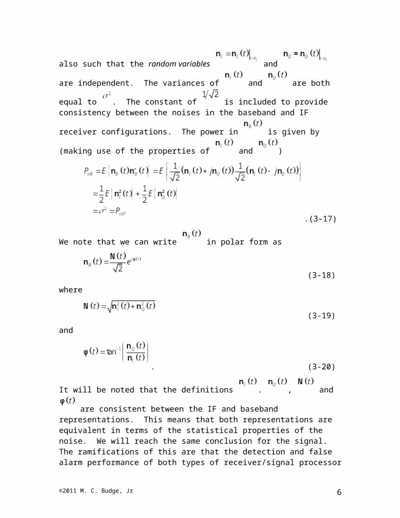
where and are joint, wide-sense stationary, zero-mean, equal variance,

Gaussian random processes. They are also such that the random variables

and are independent. The variances of and are both equal to

. The constant of is included to provide consistency between the noises in the

baseband and IF receiver configurations. The power in is given by (making use of

the properties of and )

. (3-17)

We note that we can write in polar form as

(3-18)

where

(3-19)

and

. (3-20)

It will be noted that the definitions . , and are consistent between the IF and baseband representations. This means that both representations are equivalent in terms of the statistical properties of the noise. We will reach the same conclusion for the signal. The ramifications of this are that the detection and false alarm performance of both types of receiver/signal processor configurations will be the same. Thus, the future

©2011 M. C. Budge, Jr 5

detection and false alarm probability equations that we derive will be applicable to either receiver configuration.

It should be noted that, if the receiver you are analyzing is not of one of the two forms indicated above, the ensuing detection and false alarm probability equations may not be applicable to it. The most notable exception to the two representations above is the case where the receiver uses only the I or Q channel in baseband processing. While this is not a common receiver configuration, it is sometimes used. In this case, one would need to derive a different set of detection and false alarm probability equations that would be specifically applicable to the configuration.

3.3 SIGNAL IN RECEIVERS

3.3.1 Introduction and Background

We now want to turn our attention to developing a representation of the signals at the output of the signal processor. Consistent with the noise case, we want to consider both IF and baseband receiver configurations. Thus, for our analyses we will use Figures

3-1 and 3-2 but replace with , with , with , with

and with .

We will need to develop three signal representations: one for SW0/SW5 targets, one for SW1/SW2 targets and one for SW3/SW4 targets. We have already acknowledged that the SW1 through SW4 target RCS models are random process models. To be consistent with this, and consistent with what happens in an actual radar, we will also use a random process model for the SW0/SW5 target RCS.

Since the target RCS models are random processes we must also represent the target voltage signals in the radar (henceforth termed the target signal) as random processes. To that end, the IF representation of the target signal is

(3-21)

where

(3-22)

and

. (3-23)

The baseband signal model is

. (3-24)

©2011 M. C. Budge, Jr 6

It will be noted that both of the signal models are consistent with the noise voltage model of the previous sections.

Consistent with the noise model, we assume that and are independent.2

At this point we need to develop separate signal models for the different types of

targets because the signal amplitude fluctuations, , of each are governed by different models.

3.3.2 Signal Model for SW0/SW5 Targets

For the SW0/SW5 target case we assume that the target RCS is constant. This means that the target power, and thus the target signal amplitude, will be constant. With this, we let

. (3-25)

The IF signal model becomes

. (3-26)

We introduce the random variable to force to be a random process. We

specifically choose uniform on 3. This means that and are also random

variables (rather than random processes). is a random process because of the

presence of the term.2 We have made a large number of assumptions concerning the statistical properties of the signal and noise. A natural question is: Are the assumptions reasonable? The best answer to this question is that we design radars so that the assumptions are satisfied. In particular, we endeavor to make the receiver and signal

processor linear. Because of this and the central limit theorem, we can reasonably assume that and

are Gaussian. Further, if we enforce reasonable constraints on the bandwidth of receiver components we can reasonably assume the independence requirements are valid. The stationarity requirements are easily satisfied if we assume that the receiver gains don’t change with time. We enforce the zero-mean assumption by using bandpass filters to eliminate DC components. For signals, we won’t need the Gaussian requirement. However, we will need the stationarity, zero-mean and other requirements. These are usually satisfied for signals based on the same assumptions as for noise, and by the requirement that the

target RCS is a wide sense stationary process, and that is uniform on and is wide-sense stationary. Both of the latter assumptions are valid for practical radars and targets.3 This model is actually very consistent with what happens in the actual radar. Specifically, the phase of the signal is random.

©2011 M. C. Budge, Jr 7

The density functions of and are the same and are given by

. (3-27)

We cannot assert that the random variables and are independent because we have

no means of showing that .

The signal power is given by

. (3-28)

In the above we can write

. (3-29)

Similarly, we get

(3-30)

and

. (3-31)

Substituting Equations (3-29), (3-30) and (3-31) into Equation (3-28) results in

. (3-32)

From Equation (3-24) the baseband signal model is

. (3-33)

The signal power is

©2011 M. C. Budge, Jr 8

. (3-34)

3.3.3 Signal Model for SW1/SW2 Targets

For the SW1/SW2 target case we have already stated that the target RCS is governed by the density function

. (3-35)

Since the power is a direct function of the RCS (from the radar range equations), the signal power at the signal processor output has a density function that is the same form as Equation (3-35). That is

(3-36)

where (3-37)

From random variable theory it can be shown that the signal amplitude, , is governed by the density function

. (3-38)

Which is recognized as a Rayleigh density function. This, combined with the fact that

in Equation (3-21) is uniform, and the assumption that and are independent, leads to the interesting observation that the signal model for a SW1/SW2 target is of the same form as the noise model. That is, the IF signal model for a SW1/SW2 target is of the form

(3-39)

where is Rayleigh and is uniform on . If we adapt the results from our

noise study we arrive at the conclusion that and are Gaussian with the density functions

©2011 M. C. Budge, Jr 9

. (3-40)

Furthermore, and are independent.

The signal power is given by

. (3-41)

Invoking the independence of and and the fact that and

are zero mean and have equal variances of leads to the conclusion that

. (3-42)

The baseband representation of the signal is

(3-43)

where the various terms are as defined above. The power in the baseband signal representation can be written as

(3-44)

as expected.

3.3.4 Signal Model for SW3/SW4 Targets

For the SW3/SW4 target case we have already stated that the target RCS is governed by the density function

. (3-45)

©2011 M. C. Budge, Jr 10

Since the power is a direct function of the RCS (from the radar range equation), the signal power at the signal processor output has a density function that is the same form as Equation (3-45). That is

(3-46)

where (3-47)

From random variable theory it can be shown that the signal amplitude, , is governed by the density function

. (3-48)

Unfortunately, this is about as far as we can carry the signal model development for the SW3/SW4 case. We can invoke the previous statements and write

(3-49)

and

. (3-50)

However, we don’t know the form of and . Furthermore, deriving its form has proven very laborious and elusive.

We can find the power in the signal from

. (3-51)

We will need to deal with the inability to characterize and when we consider the characterization of signal-plus-noise.

3.4 SIGNAL-PLUS-NOISE IN RECEIVERS

©2011 M. C. Budge, Jr 11

3.4.1 General Formulation

Now that we have characterizations for the signal and noise we want to develop characterizations for the sum of signal and noise. That is, we want to develop the appropriate density functions for

. (3-52)

If we are using the IF representation we would write

, (3-53)

and if we are using the baseband representation we would write

. (3-54)

In either representation, the primary variable of interest is the magnitude of the signal-

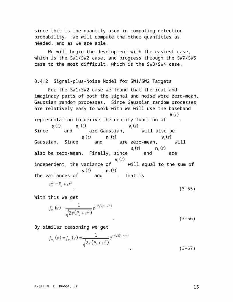
plus-noise voltage, , since this is the quantity used in computing detection probability. We will compute the other quantities as needed, and as we are able.

We will begin the development with the easiest case, which is the SW1/SW2 case, and progress through the SW0/SW5 case to the most difficult, which is the SW3/SW4 case.

3.4.2 Signal-plus-Noise Model for SW1/SW2 Targets

For the SW1/SW2 case we found that the real and imaginary parts of both the signal and noise were zero-mean, Gaussian random processes. Since Gaussian random processes are relatively easy to work with we will use the baseband representation to

derive the density function of . Since and are Gaussian, will

also be Gaussian. Since and are zero-mean, will also be zero-mean.

Finally, since and are independent, the variance of will equal to the

sum of the variances of and . That is

©2011 M. C. Budge, Jr 12

. (3-55)

With this we get

. (3-56)

By similar reasoning we get

. (3-57)

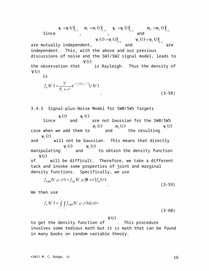
Since , , and are mutually

independent, and are independent. This, with the above and our previous discussions of noise and the SW1/SW2 signal model, leads to the

observation that is Rayleigh. Thus the density of is

. (3-58)

3.4.3 Signal-plus-Noise Model for SW0/SW5 Targets

Since and are not Gaussian for the SW0/SW5 case when we add

them to and the resulting and will not be Gaussian. This

means that directly manipulating and to obtain the density function of

will be difficult. Therefore, we take a different tack and invoke some properties of joint and marginal density functions. Specifically, we use

. (3-59)

We then use

(3-60)

©2011 M. C. Budge, Jr 13

to get the density function of . This procedure involves some tedious math but it is math that can be found in many books on random variable theory.

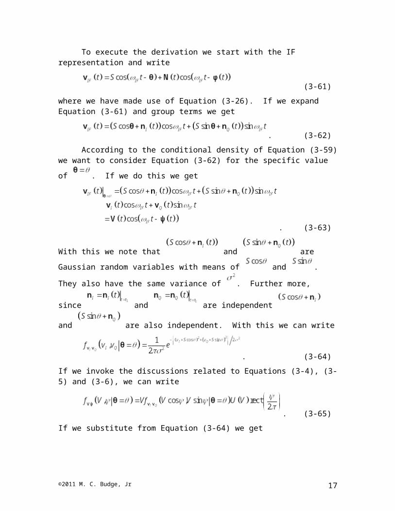
To execute the derivation we start with the IF representation and write

(3-61)

where we have made use of Equation (3-26). If we expand Equation (3-61) and group terms we get

. (3-62)

According to the conditional density of Equation (3-59) we want to consider

Equation (3-62) for the specific value of . If we do this we get

. (3-63)

With this we note that and are Gaussian random

variables with means of and . They also have the same variance of .

Further more, since and are independent and

are also independent. With this we can write

. (3-64)

If we invoke the discussions related to Equations (3-4), (3-5) and (3-6), we can write

. (3-65)

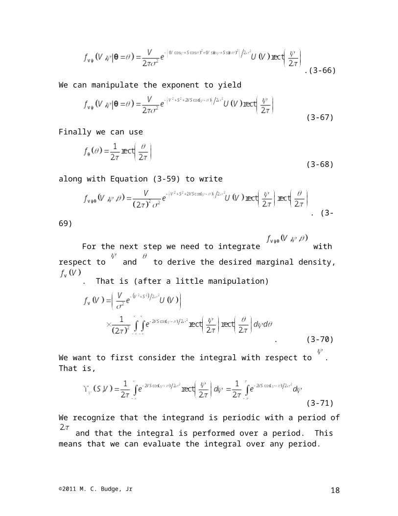
If we substitute from Equation (3-64) we get

. (3-66)

We can manipulate the exponent to yield

©2011 M. C. Budge, Jr 14

(3-67)

Finally we can use

(3-68)

along with Equation (3-59) to write

. (3-69)

For the next step we need to integrate with respect to and to

derive the desired marginal density, . That is (after a little manipulation)

. (3-70)

We want to first consider the integral with respect to . That is,

(3-71)

We recognize that the integrand is periodic with a period of and that the integral is performed over a period. This means that we can evaluate the integral over any period.

Specifically, we will choose the period from to . With this we get

. (3-72)

If we make the change of variables the integral becomes

(3-73)

©2011 M. C. Budge, Jr 15

where is a modified Bessel function of the first kind.

If we substitute Equation (3-73) into Equation (3-70) the latter becomes

(3-74)

where the last step derives from the fact that the integral with respect to is equal to

one. Equation (3-74) is the desired result, which is the density function of .

3.4.4 Signal-plus-Noise Model for SW3/SW4 Targets

As with the SW0/SW5 case, and are not Gaussian for the SW3/SW4

case. Thus, when we add them to and the resulting and will

not be Gaussian. This means that directly manipulating and to obtain the

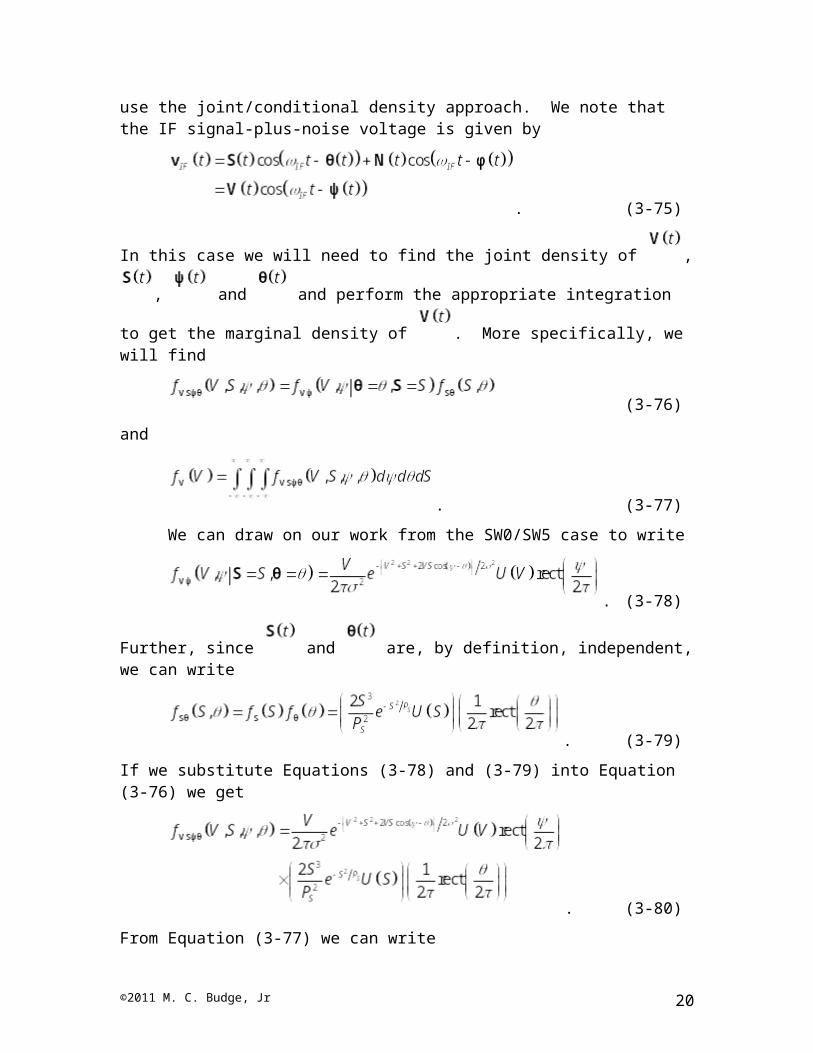
density function will be difficult. Based on our experience with the SW0/SW5 case, we will again use the joint/conditional density approach. We note that the IF signal-plus-noise voltage is given by

. (3-75)

In this case we will need to find the joint density of , , and and

perform the appropriate integration to get the marginal density of . More specifically, we will find

(3-76)

and

. (3-77)

We can draw on our work from the SW0/SW5 case to write

©2011 M. C. Budge, Jr 16

. (3-78)

Further, since and are, by definition, independent, we can write

. (3-79)

If we substitute Equations (3-78) and (3-79) into Equation (3-76) we get

. (3-80)

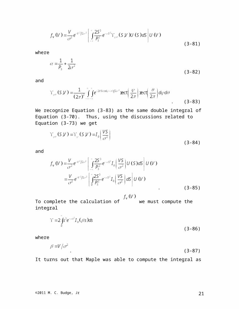
From Equation (3-77) we can write

(3-81)

where

(3-82)

and

. (3-83)

We recognize Equation (3-83) as the same double integral of Equation (3-70). Thus, using the discussions related to Equation (3-73) we get

(3-84)

and

. (3-85)

©2011 M. C. Budge, Jr 17

To complete the calculation of we must compute the integral

(3-86)

where

. (3-87)

It turns out that Maple was able to compute the integral as

. (3-88)

With this becomes

(3-89)

which, after manipulation can be written as

. (3-90)

Now that we have completed the characterization of noise, signal and signal-plus-noise we are ready to attack the detection problem.

3.5 DETECTION PROBABILITY

3.5.1 Introduction

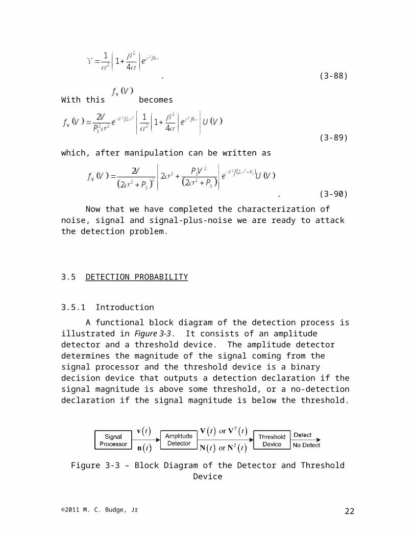
A functional block diagram of the detection process is illustrated in Figure 3-3. It consists of an amplitude detector and a threshold device. The amplitude detector determines the magnitude of the signal coming from the signal processor and the threshold device is a binary decision device that outputs a detection declaration if the signal magnitude is above some threshold, or a no-detection declaration if the signal magnitude is below the threshold.

©2011 M. C. Budge, Jr 18

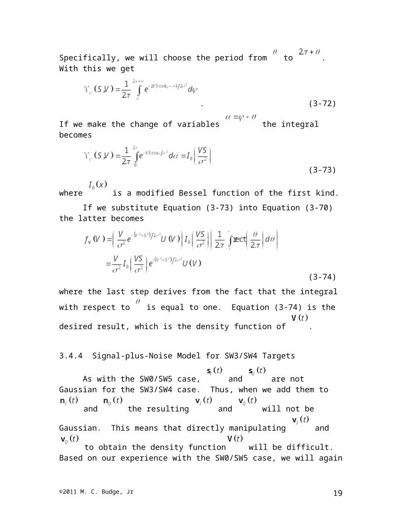
Figure 3-3 – Block Diagram of the Detector and Threshold Device

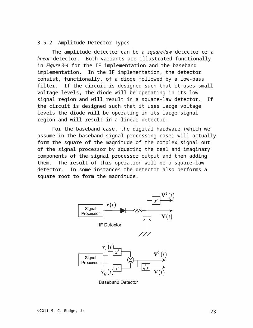
3.5.2 Amplitude Detector Types

The amplitude detector can be a square-law detector or a linear detector. Both variants are illustrated functionally in Figure 3-4 for the IF implementation and the baseband implementation. In the IF implementation, the detector consist, functionally, of a diode followed by a low-pass filter. If the circuit is designed such that it uses small voltage levels, the diode will be operating in its low signal region and will result in a square-law detector. If the circuit is designed such that it uses large voltage levels the diode will be operating in its large signal region and will result in a linear detector.

For the baseband case, the digital hardware (which we assume in the baseband signal processing case) will actually form the square of the magnitude of the complex signal out of the signal processor by squaring the real and imaginary components of the signal processor output and then adding them. The result of this operation will be a square-law detector. In some instances the detector also performs a square root to form the magnitude.

Figure 3-4 – IF and Baseband Detectors – Linear and Square Law

In either the IF or baseband representation the output of the square-law detector

will be when only noise is present at the signal processor output and when

©2011 M. C. Budge, Jr 19

signal-plus-noise is present at the signal processor output. For the linear detector the

output will be when only noise is present at the signal processor output and when signal-plus-noise is present at the signal processor output.

3.5.3 Detection Logic

Since both and are random processes we must use concepts from random processes theory to characterize the performance of the detection logic. In particular, we will use probabilities to characterize the performance of the detection logic.

Since we have two signal conditions (noise only and signal-plus-noise) and two outcomes from the threshold check we have four possible events to consider:

1. signal-plus-noise threshold – detection

2. signal-plus-noise < threshold – missed detection

3. noise threshold – false alarm

4. noise < threshold – no false alarm

Of the above, the two desired events are 1 and 4. That is, we want to detect targets when they are present and we don’t want to detect noise when targets are not present. Since events 1 and 2 are related and events 3 and 4 are related we only find probabilities associated with events 1 and 3. We term the probability of the first event occurring the detection probability and the probability of the third even occurring the false alarm probability. In equation form

(3-91)

and

. (3-92)

where is the signal-plus-noise voltage evaluated at a specific time and

is the noise voltage evaluated at a specific time.

The above definition carries some subtle implications. First, when one finds detection probability it is tacitly assumed that the target return is present at the time the output of the threshold device is checked. Likewise, when one finds false alarm probability it is tacitly assumed that the target return is not present at the time the output of the threshold device is checked.

In practical applications it is more appropriate to say: At the time the output of the threshold device is checked the probability that there will be a threshold crossing is equal

©2011 M. C. Budge, Jr 20

to if the signal contains a target signal and if the signal does not contain a target signal. In typical applications the output of the threshold device will be checked at times separated by a pulse width and will result in many checks per PRI.

It will be noted that the above probabilities are conditional probabilities. In normal practice we don’t explicitly use the conditioning and write

(3-93)

and

(3-94)

and recognize that we should use signal-plus-noise when we assume the target is present and noise only when we assume that the target is not present.

The above assumes that the detector preceding the threshold device is a linear detector. If the detector is a square law detector the appropriate equations would be

(3-95)

and

. (3-96)

3.5.4 Calculation of and

From probability theory we can write

or (3-97)

and

or (3-98)

In the above is the threshold voltage level and is the threshold expressed as normalized power.

To avoid having to use two sets of and equations we will digress to show that we can compute them using either of the integrals of Equations (3-97) and (3-98).

©2011 M. C. Budge, Jr 21

It can be shown4 that if and then

. (3-99)

If we write

(3-100)

we can use Equation (3-99) to write

. (3-101)

If we make the change of variables we can write

. (3-102)

Similar results apply to and indicate that one can use either form to compute detection and false alarm probability.

If we examine the equations for and we note that both are integrals over the same limits. This integration is illustrated graphically in Figure 3-5. It will be noted

that and are areas under their respective density functions to the right of the threshold value. Thus, increasing the threshold decreases the probabilities and decreasing the threshold increases the probabilities. This is not exactly what we want. Ideally, we

want to select the threshold so that we have and . However this is not possible and we therefore usually choose the threshold as some sort of tradeoff between

and . In fact, what we actually do is choose the threshold to achieve a certain

and find other means of increasing .

If we refer to Equation (3-12) the only parameter that affects is the noise

power, . While we have some control over this via noise figure and effective noise

bandwidth, executing this control can be very expensive. On the other hand, is 4 Papoulis, A. “Probability, Random Variables, and Stochastic Processes” McGraw-Hill

©2011 M. C. Budge, Jr 22

dependent upon both and . Thus, this gives us some degree of control. In fact,

what we usually try to do is affect both and by increasing and

decreasing . The net result of this is that we try to maximize SNR.

Figure 3-5 – Probability Density Functions for Noise and Signal-plus-noise

3.5.4.1 False Alarm Probability

If we use Equation (3-12) in Equation (3-98) we get

. (3-103)

In this equation we define

(3-104)

©2011 M. C. Budge, Jr 23

as the threshold-to-noise ratio. As indicated earlier, we usually select a desired and, from this derive the required TNR as

. (3-105)

3.5.4.2 Detection Probability

We can compute detection probability for the three target classes by substituting Equations (3-58), (3-74) and (3-90) into Equation (3-102). The results for SW0/SW5 targets is

. (3-106)

where

(3-107)

is the signal-to-noise ratio that one would compute from the radar range equation and

(3-108)

is one form of the error function.5

The detection probability equations for the SW1/SW2 case and for the SW3/SW4 case are, respectively

(3-109)

and

. (3-110)

In Equations (3-109) and (3-110) SNR is the signal-to-noise ratio computed from the radar range equation.

5 This Equation (3-106) should only be used for cases where SNR is larger than TNR.

©2011 M. C. Budge, Jr 24

3.5.5 Behavior vs. Target Type

Figure 3-6 contains plots of versus SNR for the three target types and

, a typical value. It is interesting to note the behavior for the three target

types. In general, the SW0/SW5 target provides the largest for a given SNR, the

SW1/SW2 target provides the lowest and the SW3/SW4 is somewhere between the other two. With some thought this makes sense. For the SW0/SW5 target model the only thing affecting a threshold crossing is the noise (since the RCS of the target is constant). For the SW1/SW2 the target RCS can fluctuate considerably, thus both noise and RCS fluctuation affects the threshold crossing. The standard assumption for the SW3/SW4 model is that it consists of a predominant (presumably constant RCS) scatterer and several smaller scatterers. Thus, the threshold crossing for the SW3/SW4 target is affected somewhat by RCS fluctuation, but not to the extent of the SW1/SW2 target.

It is interesting to note that the SNR required for , with , on a

SW1/SW2 target is about 13 dB. This same SNR gives a on a SW0/SW5 target.

To obtain a on a SW1/SW2 target requires a SNR of about 21 dB. These numbers are the origin of the 13 dB and 20 dB SNR numbers we used in our radar range equation studies.

©2011 M. C. Budge, Jr 25

Figure 3-6 - vs. SNR for Three Target Types and

3.6 DETERMINATION OF FALSE ALARM PROBABILITY

One of the parameters in the detection probability equations is threshold-to-noise

ratio, . As indicated in Equation (3-105), , where is the false alarm probability. False alarm probability is set by system requirements.

In a radar, false alarms result in wasted radar resources (energy, timeline and hardware) in that every time a false alarm occurs the radar must expend resources determining that it did, in fact, occur. Said another way, every time the output of the

©2011 M. C. Budge, Jr 26

amplitude detector exceeds the threshold, , a detection is recorded. The radar data processor does not know, a priori, whether the detection is a target detection or the result of noise (i.e. a false alarm). Therefore, the radar must verify each detection. This usually requires transmission of another pulse and another threshold check (an expenditure of time and energy). Further, until the detection is verified, it must be carried in the computer as a valid target detection (an expenditure of hardware).

In order to minimize wasted radar resources we wish to minimize the probability

of a false alarm. Said another way, we want to minimize . However, we can’t set

to an arbitrarily small value because this will increase and reduce detection

probability, (see Equations (3-106), (3-109) and (3-110)). As a result we set to provide an acceptable number of false alarms within a given time period. This last

statement provides the criterion normally used to compute . Specifically, one states

that is chosen to provide an average of one false alarm within a time period that is

termed the false alarm time , . is usually set by some criterion that is driven by radar resource limitations.

The classical method of determining is based strictly on timing. This can be explained with the help of Figure 3-7 which contains a plot of noise at the output of the amplitude detector. The horizontal line labeled “Threshold, T” represents the detection threshold voltage level. It will be noted that the noise voltage is above the threshold for

three time intervals of length , and . Further, the spacings between threshold

crossings are and . Since a threshold crossing constitutes a false alarm one can say

that over the interval false alarms occur for a period of . Likewise, over the interval

false alarms occur for a period of , and so forth. If we were to average all of the

we would have the average time that the noise is above the threshold, . Likewise, if we

were to average all of the we would have the average time between false alarms; i.e.

the false alarm time, . To get the false alarm probability we would take the ratio of

to , i.e.

. (3-111)

©2011 M. C. Budge, Jr 27

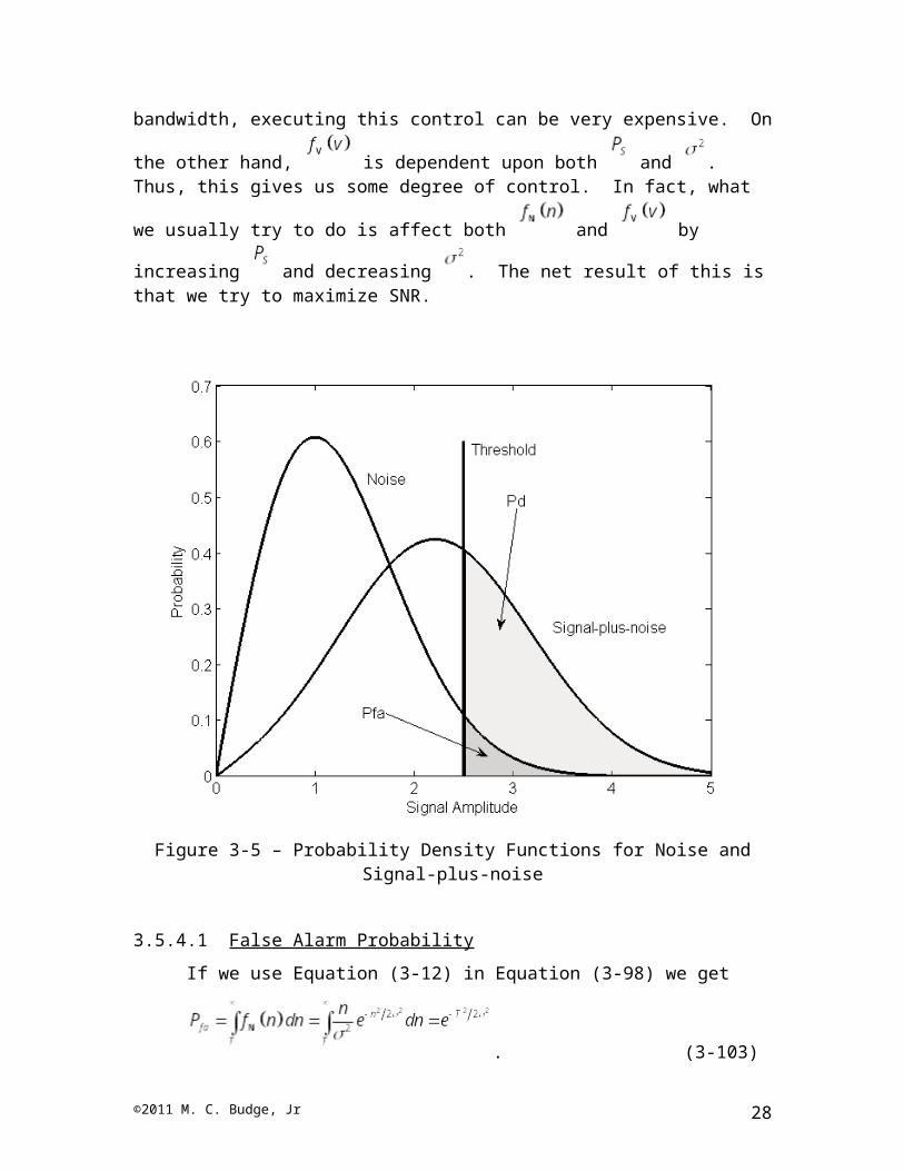
Figure 3-7 – Illustration of False Alarm Time

While is reasonably easy to specify, the specification of is not obvious.

The standard assumption is to set to the range resolution expressed as time, . For

an unmodulated pulse, is the pulse width. For a modulated pulse, is the reciprocal of the modulation bandwidth.

It has been the author’s experience that the above method of determining not very accurate. While it would be possible to place the requisite number of caveats on Equation (3-111) to make it accurate, with modern radars this is not necessary.

The previously described method of determining was based on the assumption that detections were recorded via hardware operating on a continuous-time signal. In modern radars, detection is based on examining signals that have been converted to the discrete-time domain by sampling or by and analog-to-digital converter.

This makes determination of easier, and more intuitively appealing, in that one can deal with discrete events. With modern radars one computes the number of false alarm

chances, , within the desired false alarm time, , and computes the probability of false alarm from

. (3-112)

To compute one needs to know certain things about the operation of the radar. We will outline some thoughts along this line.

©2011 M. C. Budge, Jr 28

In a typical radar, the return signal from each pulse is sampled with a period equal

to the range resolution, , of the pulse. As indicated above, this would be equal to the pulse width for an unmodulated pulse and the reciprocal of the modulation bandwidth for a modulated pulse. These range samples are usually taken over the instrumented range,

. In a search radar, might be only slightly less than the PRI, . However, for a

track radar, , may be significantly less than . With the above, we can compute the number of range samples per PRI as

. (3-113)

Each of the range samples provides a chance that a false alarm will occur.

In a time period of the radar will transmit

(3-114)

pulses. Thus, the number of range samples (and thus chances for false alarm) that one

has over the time period of is

. (3-115)

In some radars, the signal processor consists of several ( ), parallel Doppler

channels. This means that it will also contain amplitude detectors. Each amplitude

detector will generate range samples per PRI. Thus, in this case, the total number of

range samples in the time period would be

. (3-116)

In either case, the false alarm probability would be give by Equation (3-112).

3.6.1 Example

To illustrate the above, we consider a simple example. We have a search radar

that has a PRI of . It uses a pulse with linear frequency modulation

(LFM) where the LFM bandwidth is 1 MHz. With this we get . We assume

©2011 M. C. Budge, Jr 29

that the radar starts its range samples one pulse-width after the transmit pulse and stops taking range samples one pulse-width before the succeeding transmit pulse. From this we

get . The signal processor is not a multi-channel Doppler processor. The

radar has a search scan time of and we desire no more than one false alarm every two scans.

From the last sentence above we get . If we combine this with the PRI we get

. (3-117)

From and we get

. (3-118)

This results in

(3-119)

and

. (3-120)

©2011 M. C. Budge, Jr 30