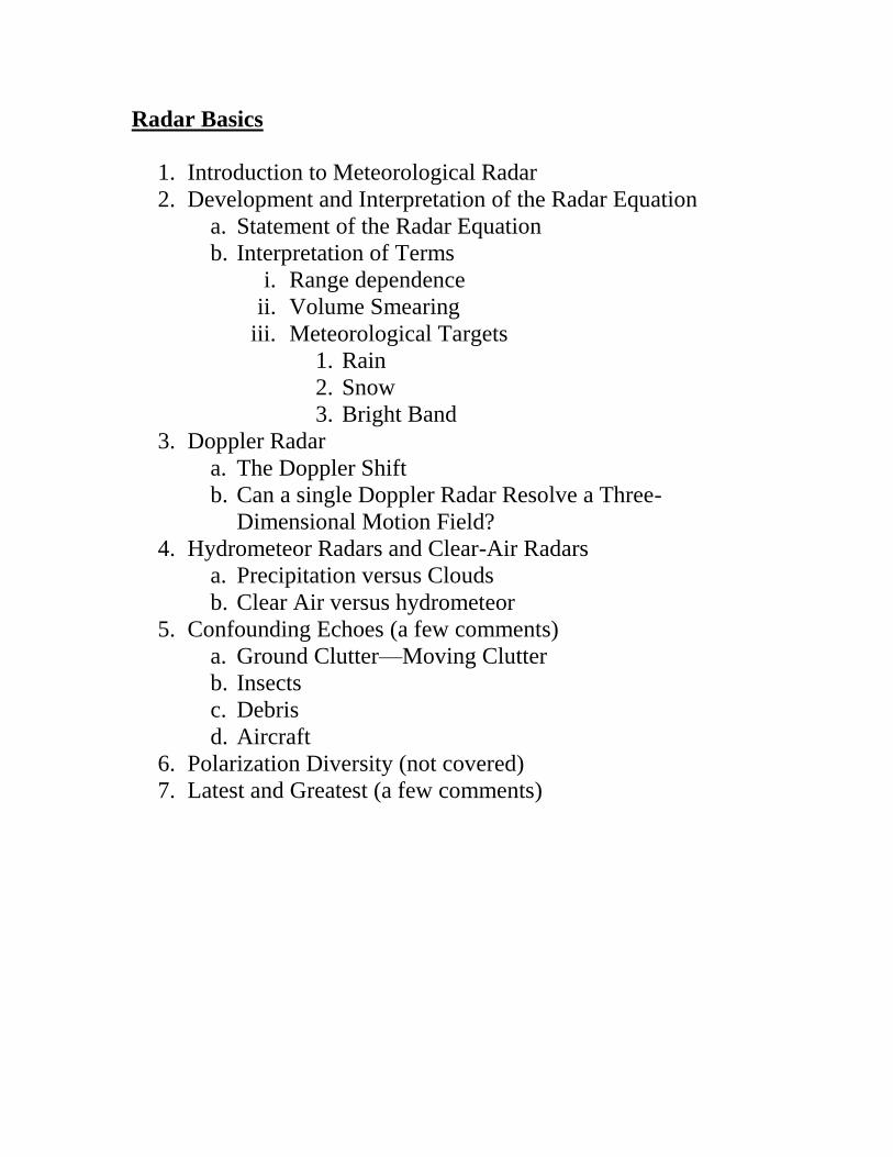
Radar Basics

1. Introduction to Meteorological Radar

2. Development and Interpretation of the Radar Equation

a. Statement of the Radar Equation

b. Interpretation of Terms

i. Range dependence

ii. Volume Smearing

iii. Meteorological Targets

1. Rain

2. Snow

3. Bright Band

3. Doppler Radar

a. The Doppler Shift

b. Can a single Doppler Radar Resolve a Three-

Dimensional Motion Field?

4. Hydrometeor Radars and Clear-Air Radars

a. Precipitation versus Clouds

b. Clear Air versus hydrometeor

5. Confounding Echoes (a few comments)

a. Ground Clutter—Moving Clutter

b. Insects

c. Debris

d. Aircraft

6. Polarization Diversity (not covered)

7. Latest and Greatest (a few comments)

1. Introduction to Meteorological Radar

RADAR=RAdio Detecting And Ranging

Although the development of radar as a full-fledged technology

did not occur until WWII, the basic principal of radar detection is

almost as old as the subject of electromagnetism itself.

Heinrich Hertz, in 1886, experimentally tested the theories

of Maxwell and demonstrated that radio waves could be

reflected by metallic and dielectric bodies (non-conductor of

electricity).

In 1903, a German engineer named Hulsmeyer experimented

with the detection of radio waves reflected from ships and

obtained a patent for an obstacle detector and ship

navigational device. The German Navy showed no interest

in the invention!

In 1922, an excerpt from Marconi’s lecture to the Institute of

radio Engineers states: “It seems to me that it should be

possible to design an apparatus by means of which a ship

could radiate or project a divergent beam of these rays in any

desired direction, which rays, if coming across a metal

object, such as a steamer or ship, would be reflected back to

a receiver screened from the local transmitter on the sending

ship, and thereby, immediately reveal the presence and

bearing of the other ship in fog or thick weather”.

Marconi’s suggestion motivated Taylor and Young of the

Naval Research Laboratory to confirm experimentally the

speculations by detecting a wooden ship. A proposal to

develop this technology was refused!

The first use of pulsed radar technique to measure distance

was by Breit and Tuve, in 1925.

The first radar detection of aircraft was in 1930 by L.A.

Hyland of the Naval Research Laboratory (NRL). It was

made accidentally while he was working with a direction-

finding, continuous wave apparatus installed on an aircraft

on the ground.

NRL started the development of pulse radar in 1934 through

the efforts of R.M. Page, but he was not allowed to devote

his full effort to the project!

In 1935, NRL successfully tested pulsed radar with a range

of 25-miles.

Nineteen pulsed radars were installed on ships in 1941.

2. Development and Interpretation of the Radar Equation

Photons are the basic components of an Electromagnetic Wave

(EM waves hereafter).

The simplest source of EM waves is a dipole radiator, which

consists of an object subjected to an oscillating electric field

that reverses its polarity on a regular basis. A dipole antenna is

a length of electrically conducting material (metal) that has its

polarity artificially changed by an attached electric circuit

designated as a generator. A generator attached to an infinite,

loss-less wire, which is often referred to as a transmission line,

produces a uniform traveling wave along the line. If the line

abruptly ends (is short circuited), the outgoing traveling wave is

reflected back toward the generator and produces a standing

wave on the transmission line due to the interference between

the incoming and outgoing waves. A standing wave may be

viewed as a distribution of energy along the transmission line

that causes the standing wave to oscillate from entirely electric

to entirely magnetic and back twice per oscillation cycle. This

behavior is characteristic of a resonant circuit and this

concentration of energy that always exists as a consequence of

the standing wave is a form of stored energy. When the amount

of stored energy greatly exceeds the net energy flow per cycle

this system is known as a resonator. If the wave is enclosed in

a waveguide, which is like a pipe for EM waves, or other

enclosure with conducting characteristics, and the waveguide or

enclosure is terminated at one end, the resonance and energy

storage are confined to the cavity inside the waveguide, and

referred to as a cavity resonator. Such cavity resonators form

the basis for many radar transmitters.

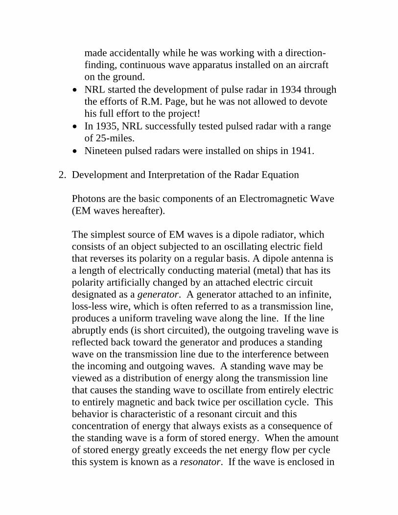
Antennas are the interface between a guided wave and a free

space wave. They radiate and receive energy, while

transmission lines (sometimes referred to as waveguides) guide

energy and resonators store energy. Antennae convert the

photons that comprise an EM wave into moving electrons

within an electric circuit, or currents, and vice versa. Consider

the configuration shown below in which a transmission line is

connected to a dipole antenna, which emits a free space wave.

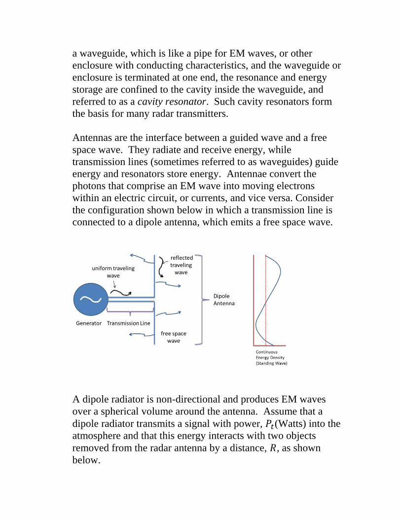
A dipole radiator is non-directional and produces EM waves

over a spherical volume around the antenna. Assume that a

dipole radiator transmits a signal with power, (Watts) into the

atmosphere and that this energy interacts with two objects

removed from the radar antenna by a distance, , as shown

below.

Because is spread over a spherical surface, which has surface

area where the distance from the dipole source is , we

can compute the amount of the transmitted power that is

delivered to any area on the sphere, or the power density.

Power Density from an Omni-directional Antenna in a non-

absorbing atmosphere

24

)(

R

WattsPt

R is the Range to the Target

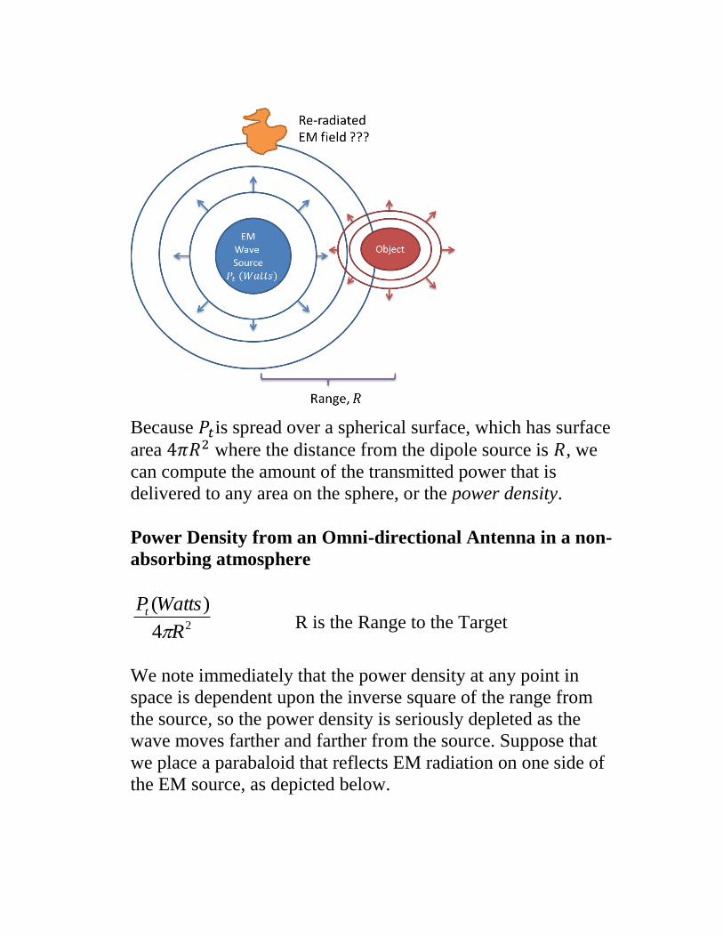
We note immediately that the power density at any point in

space is dependent upon the inverse square of the range from

the source, so the power density is seriously depleted as the

wave moves farther and farther from the source. Suppose that

we place a parabaloid that reflects EM radiation on one side of

the EM source, as depicted below.

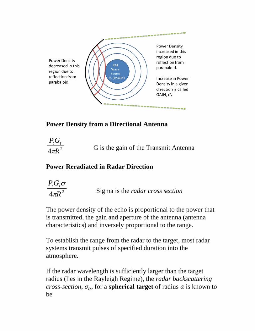
Power Density from a Directional Antenna

24 R

GP tt

G is the gain of the Transmit Antenna

Power Reradiated in Radar Direction

24 R

GP tt

Sigma is the radar cross section

The power density of the echo is proportional to the power that

is transmitted, the gain and aperture of the antenna (antenna

characteristics) and inversely proportional to the range.

To establish the range from the radar to the target, most radar

systems transmit pulses of specified duration into the

atmosphere.

If the radar wavelength is sufficiently larger than the target

radius (lies in the Rayleigh Regime), the radar backscattering

cross-section, , for a spherical target of radius is known to

be

| |

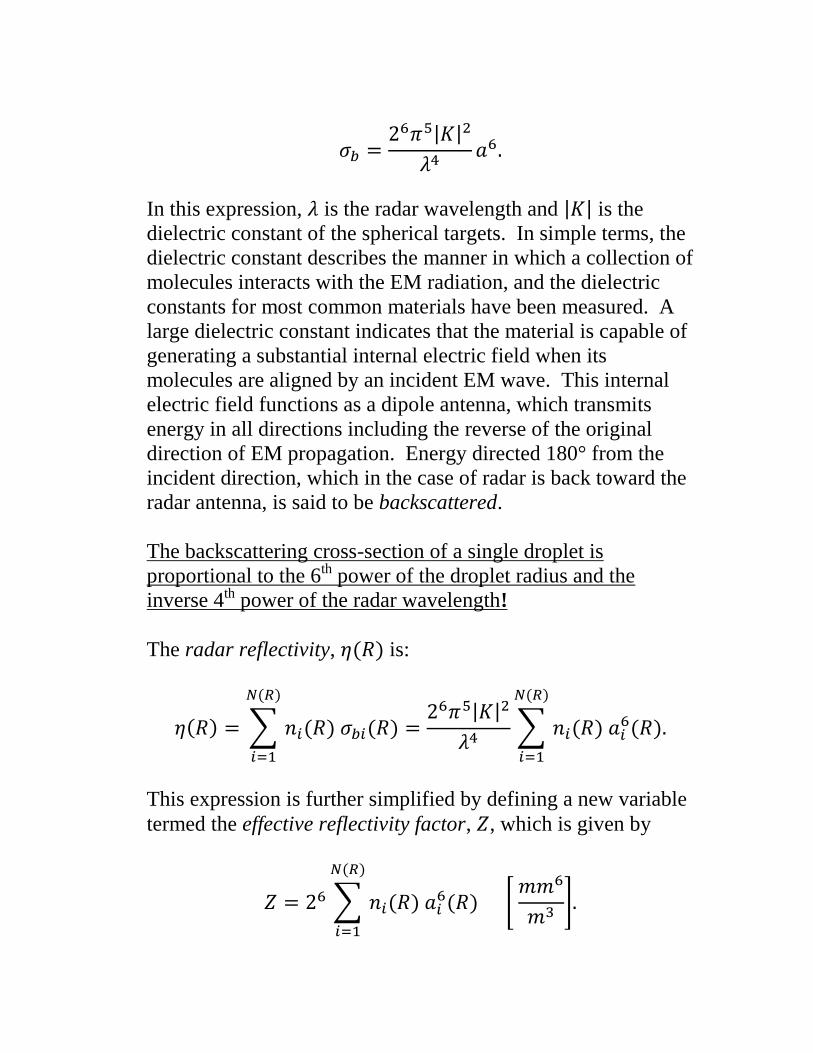
In this expression, is the radar wavelength and | | is the

dielectric constant of the spherical targets. In simple terms, the

dielectric constant describes the manner in which a collection of

molecules interacts with the EM radiation, and the dielectric

constants for most common materials have been measured. A

large dielectric constant indicates that the material is capable of

generating a substantial internal electric field when its

molecules are aligned by an incident EM wave. This internal

electric field functions as a dipole antenna, which transmits

energy in all directions including the reverse of the original

direction of EM propagation. Energy directed 180° from the

incident direction, which in the case of radar is back toward the

radar antenna, is said to be backscattered.

The backscattering cross-section of a single droplet is

proportional to the 6th power of the droplet radius and the

inverse 4th power of the radar wavelength!

The radar reflectivity, is:

∑

| |

∑

This expression is further simplified by defining a new variable

termed the effective reflectivity factor, , which is given by

∑

[

]

Note that the variables that are summed define the Droplet Size

Distribution (DSD) and the definition of combines two

unknowns into a single “catch-all” variable. Defining as a

new variable is necessary because there is only one

measureable quantity at the radar receiver, which is , and

hence there is no way to determine the independent

contributions of and to .

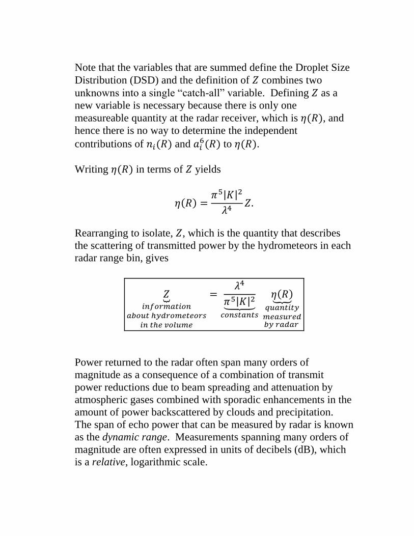
Writing in terms of yields

| |

Rearranging to isolate, , which is the quantity that describes

the scattering of transmitted power by the hydrometeors in each

radar range bin, gives

⏟

| | ⏟

⏟

Power returned to the radar often span many orders of

magnitude as a consequence of a combination of transmit

power reductions due to beam spreading and attenuation by

atmospheric gases combined with sporadic enhancements in the

amount of power backscattered by clouds and precipitation.

The span of echo power that can be measured by radar is known

as the dynamic range. Measurements spanning many orders of

magnitude are often expressed in units of decibels (dB), which

is a relative, logarithmic scale.

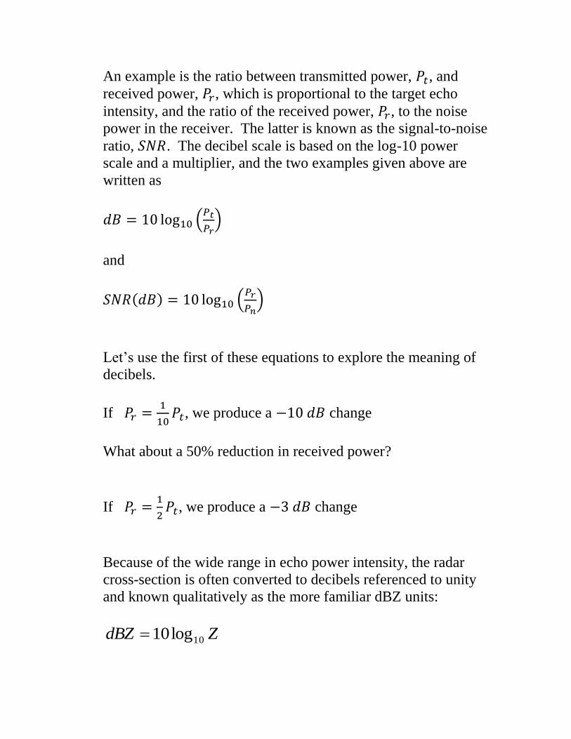
An example is the ratio between transmitted power, , and

received power, , which is proportional to the target echo

intensity, and the ratio of the received power, , to the noise

power in the receiver. The latter is known as the signal-to-noise

ratio, . The decibel scale is based on the log-10 power

scale and a multiplier, and the two examples given above are

written as

(

)

and

(

)

Let’s use the first of these equations to explore the meaning of

decibels.

If

, we produce a change

What about a 50% reduction in received power?

If

, we produce a change

Because of the wide range in echo power intensity, the radar

cross-section is often converted to decibels referenced to unity

and known qualitatively as the more familiar dBZ units:

ZdBZ 10log10

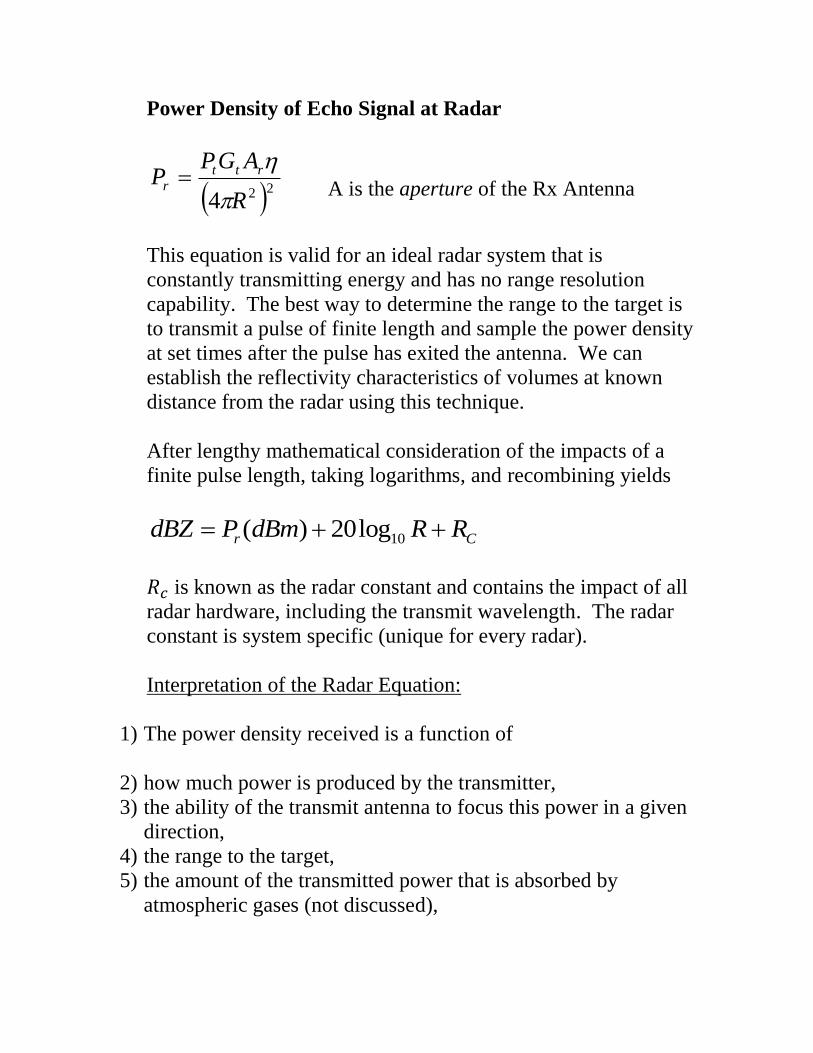
Power Density of Echo Signal at Radar

224 R

AGPP rtt

r

A is the aperture of the Rx Antenna

This equation is valid for an ideal radar system that is

constantly transmitting energy and has no range resolution

capability. The best way to determine the range to the target is

to transmit a pulse of finite length and sample the power density

at set times after the pulse has exited the antenna. We can

establish the reflectivity characteristics of volumes at known

distance from the radar using this technique.

After lengthy mathematical consideration of the impacts of a

finite pulse length, taking logarithms, and recombining yields

10( ) 20logr CdBZ P dBm R R

is known as the radar constant and contains the impact of all

radar hardware, including the transmit wavelength. The radar

constant is system specific (unique for every radar).

Interpretation of the Radar Equation:

1) The power density received is a function of

2) how much power is produced by the transmitter,

3) the ability of the transmit antenna to focus this power in a given

direction,

4) the range to the target,

5) the amount of the transmitted power that is absorbed by

atmospheric gases (not discussed),

6) the ratio between the inverse fourth power of the wavelength of

the transmitted power and the sum of the individual return

power densities of each droplet within the volume of

atmosphere that is being illuminated. The return power of each

droplet varies according to the 6th power of the droplet radius,

and

a) the aperture (~gain) of the receive antenna.

7) The ability of the radar receiver to detect a return signal that can

be discerned from the power density of thermal noise within the

receiver electronics is determined by

a) the noise level,

b) the received power density, and

c) the number of pulses that we can average (not discussed).

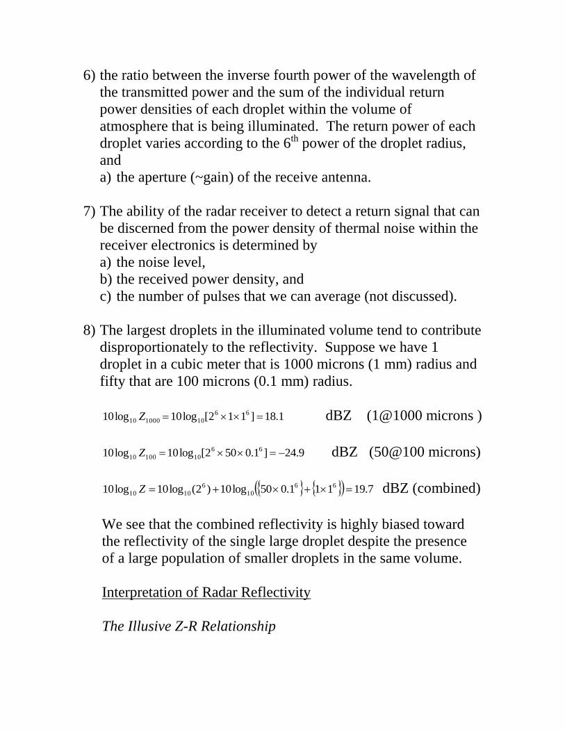
8) The largest droplets in the illuminated volume tend to contribute

disproportionately to the reflectivity. Suppose we have 1

droplet in a cubic meter that is 1000 microns (1 mm) radius and

fifty that are 100 microns (0.1 mm) radius.

1.18]112[log10log10 66

10100010 Z dBZ (1@1000 microns )

9.24]1.0502[log10log10 66

1010010 Z dBZ (50@100 microns)

7.19111.050log10)2(log10log10 66

10

6

1010 Z dBZ (combined)

We see that the combined reflectivity is highly biased toward

the reflectivity of the single large droplet despite the presence

of a large population of smaller droplets in the same volume.

Interpretation of Radar Reflectivity

The Illusive Z-R Relationship

Radar literature is replete with all manner of expressions that

attempt to relate radar reflectivity to the rainfall rate. The

equations that attempt this magic are called Z-R relationships

and they are often reported as power-law relationships of the

following form:

pARZ

In a typical Z-R relationship, A is a constant, R is the rainfall

rate in arbitrary units, and p is a positive real number (decimal).

There are dozens of Z-R relationships in the literature.

The flux of water (rainfall rate) through a horizontal plain (like

the surface) depends upon the spectrum of droplet sizes because

different droplet sizes have different fall velocities. The basic

problem encountered when trying to relate radar reflectivity

with the rainfall rate is that the radar reflectivity is proportional

to the 6th power of the droplet radius, the water content of the

droplets in the volume is proportional to the 3rd power of the

droplet radius, and the fall velocity of raindrops drops is

approximately inversely proportional to the 1st power droplet

radius. If the fall velocity and liquid water content were to be

proportional to the 6th power of the droplet size, as is the radar

reflectivity, it would be possible to relate the radar reflectivity

directly to the rainfall rate without specific knowledge of the

spectrum of droplet sizes in the volume.

How do we beat the basic laws of physics? We measure the

radar reflectivity above a point on the surface where the rainfall

rate is being measured by a rain gauge and we plot the data on a

graph. We fit these data to a power law relationship (of the

form above) and use this relationship to map radar reflectivity

into rainfall rates. How can such a technique be successful in

light of the physical arguments given above? Well, it is

because to first order, the rainfall rate is primarily a function of

the largest droplets in the sample volume. The largest drops

carry the bulk of the water and have the largest fall velocities,

and therefore, contribute the most to the observed rainfall rate.

Why are there so many different Z-R relationships? This is

because the type and characteristic of precipitation varies

widely from location to location on the planet, so local

meteorologists often develop a “tuned” Z-R relationship for

their region.

All hope is not lost, however, because the National Weather

Service has recognized that Z-R relationships are futile, for the

most part, and use rain gauges to “calibrate” the radars on an

hourly basis. In other words, they use the radar data as a means

to “upscale” calibrated data from a few spots.

There are also Z-R relationships for snow, but they are on much

shakier fundamental footing than those for rain. The reason is

that the radar backscattering cross section for snow is complex

and difficult to determine. It varies widely from case to case

(How many different configurations of snow have you seen?)

and is temperature dependent.

The Radar Bright Band

When snow melts into rain, the region where this melting

occurs often has a stronger reflectivity than snow above or

rain below; this region was hence given the name of

"bright band".

The bright band occurs just below the height of the 0°C

level. Snow falls is composed of pure ice that is often

falling in an oriented configuration, so its radar reflectivity

if much lower that that of an “equivalent sphere” of liquid

water.

When snowflakes encounter the 0°C isotherm, they begin

to melt. The surface of the snowflake becomes wet

causing snow flakes to “clump” together into large

aggregates. As the melting proceeds, a liquid spherical

shell is formed around the remaining ice. Because ice is

less dense than liquid, these “spongy wet spheres” have a

larger size (radar cross section) than the same mass of pure

liquid.

As the ice at the core of the spongy wet droplet melts, the

droplet “compresses” and accelerates toward the surface.

Exceptionally large “clumps” of wet snowflakes evolve

into rain drops that are too large to be dynamically stable.

When this occurs, these large droplets divide into smaller

droplets and their radar reflectivity is reduced.

Doppler Radar

Assume that a target is at a range, r, from a radar operative at a

frequency, f0 (corresponding to wavelength, λ). The total

distance traversed by an impulse (narrow pulse) in going to the

target and back to the antenna obviously is 2r.

Measured in terms of wavelength, the distance is 2r/ λ or, in

radians

2 / 2 4 / ( )r r radians

If the electromagnetic wave emitted by the antenna has a phase

φ0, the phase after it returns will be

r40

The change in phase as a function of time (from one pulse to the

next) is

dt

dr

dt

d

4

If the target at range r is moving along the radar beam axis, the

target velocity is

dt

drV

The angular frequency is:

fdt

d

2

Making these two substitutions gives:

Vf

2

where f is the Doppler shift frequency and V is the radial

velocity of the target, also called the “Doppler Velocity”.

It must always be remembered that the Doppler velocity

measured by the radar is only a component of the actual wind -

the part that is blowing towards or away from the radar. The

radar cannot measure the "crosswise" component. The actual

wind will be at least as strong as the Doppler velocity, and

possibly considerably stronger.

Hydrometeor Radars and Clear-Air Radars

Let’s recall that “Heinrich Hertz, in 1886, experimentally tested

theories of Maxwell and demonstrated that radio waves could

be reflected by metallic and dielectric bodies (non-conductor of

electricity).”

In free space electromagnetic waves propagate in straight lines

because everywhere the dielectric permittivity and magnetic

permeability are the same (constants related to the speed of

propagation, actually).

The Earth’s atmosphere has larger permittivity than free space

and its permittivity is vertically stratified, so microwaves travel

in curved paths at speeds less than the speed of light.

Sometimes their paths are so convoluted that they are bent back

to the surface by this stratification. The path of a radar signal is

determined by the change in height of the Earth’s refractive

index, n, which is a function of vertical gradients in

temperature, pressure, and water vapor.

It can be shown that local variations in the refractive index give

rise to the scattering of microwave signals!

The intensity of the scattering that is accomplished by these

local gradients is a function of the strength of the temperature,

pressure, or water vapor gradient and upon the strength of the

turbulent eddies that are deforming it. Depending on the

intensity of the echoes from other targets in the scattering

volume, the scattered energy from the refractive gradients

generated by turbulent eddies of a given size (inertial subrange)

may be detected by the radar receiver and the Doppler velocity

measured.

Radar backscatter from turbulent eddies that have wavelengths

that are one-half the transmitted wavelength can produce

detectable signals at the antenna due to constructive

interference (Bragg Scatter).

The refractive index structure parameter, Cn, which depends

primarily on fluctuations in the moisture field, is used to

quantify the scattering. The radar reflectivity that results from

fluctuations in the moisture field is

2 11/3 2 4

e n nZ AC AC

where

25

0.38

w

AK

This equation that quantifies clear-air (not precipitating) echoes

whose Doppler velocity can be measured. As the radar

wavelength increases, the reflectivity of moisture fluctuations

gets larger. Conversely, as the radar wavelength increases, the

echoes from hydrometeors decrease at approximately the same

rate, which is λ4!

About Marconi:

In 1895 Italian inventor Guglielmo Marconi built the

equipment and transmitted electrical signals through the air

from one end of his house to the other, and then from the house

to the garden. These experiments were, in effect, the dawn of

practical wireless telegraphy or radio.

Marconi built a transmitter, 100 times more powerful than any

previous station, at Poldhu, on the southwest tip of England,

and in November 1901 installed a receiving station at St. John's

Newfoundland.