Racial Diversity and Macroeconomic Productivity

across US States and Cities∗

Chad Sparber

Colgate University

13 Oak Drive

Hamilton, NY 13346

csparber@mail.colgate.edu

Revised: November 2007

Abstract

The United States is growing increasingly diverse, so it is important that econo-

mists understand the macroeconomic consequences of diversity within the US economy.

International analyses often argue that heterogeneity reduces macroeconomic produc-

tivity by engendering corruption, political instability, and social turmoil. However,

other studies claim that diversity improves creative decision making and augments

productivity. This paper exploits differences in diversity across regions of the United

States from 1980 to 2000 to determine whether racial heterogeneity creates macroeco-

nomic gains or losses for states and cities. Fixed effects analysis indicates that diversity

enhances the productivity of cities. Evidence at the state-level is more ambiguous, as

significant results only appear in random effects specifications.

Key Words: Racial Diversity, Macroeconomic Productivity

JEL Classification Codes: O40, R11, J24, O51

∗I would like to acknowledge the guidance and advice from three anonymous referees and the faculty andstudents of Colgate University, Union College, and the University of California — Davis. I especially thankGiovanni Peri, Hilary W. Hoynes, Alan M. Taylor, Florence Bouvet, Takao Kato, and Ahmed S. Rahman.A fellowship from the University of California Office of the President provided support for this research.

1

1 Introduction

The United States population has become increasingly diverse over the past several decades.

Whites declined from 84% of national employment in 1980 to just 74% twenty years later.

The US Census Bureau expects that Whites will cease to represent a majority racial group

shortly after 2050.1 Still, some regions remain far more diverse than others. No majority

group resided in California or New Mexico in 2000, but minorities composed less than 5% of

the populations of Maine, Vermont, and New Hampshire. That same year, Whites made up

80-90% of employees within the major metropolitan areas of Saint Louis, Minneapolis, and

Boston, while they constituted only a 44% minority in Los Angeles and San Antonio.2

Economists, psychologists, and sociologists have discovered many implications of in-

creased racial diversity. International macroeconomists began to consider the consequences

of diversity in the mid 1990s, largely focusing upon the ill effects of ethnic conflict, insti-

tutional inefficiency, political instability, social conflict, lack of trust, and civil war.3 Other

social scientists, however, have argued that people from varied groups may be unique factors

of production that could complement each other so that diversity facilitates productivity

gains. The net effects of these costs and benefits of diversity on US economic performance

remain unclear. Current demographic trends warrant further analysis of the connection be-

tween racial diversity and macroeconomic productivity in the United States. This paper

employs a decennial panel dataset covering 1980, 1990, and 2000 to assess the aggregate

economic effects of diversity on US states and cities.

Section 2 begins with a detailed review of previous research. Importantly, this section

discusses the channels through which diversity could affect productivity, though the subse-

quent empirical analysis does not attempt to assess the validity of these channels. Section 3

defines racial diversity and its measurement. Sections 4 and 5 perform the empirical analy-

sis. The former focuses on state performance. US state-level analysis is the most obvious

counterpart to diversity research from the international economics literature. Unfortunately,

however, evidence across states for the gains or losses from diversity is limited. Random

effects estimation implies that a one standard deviation increase in diversity can lead to an

approximate 5.9% rise in gross state output per worker, but fixed effects analysis fails to

uncover any causal effects. Section 5 conducts city-level analysis as an alternative. This has

the advantage of increasing the number of observations available. Moreover, this methodol-

ogy may be more appropriate if cities are the centers of economic activity in the US. The

limitation, however, is that output per worker measures are not available for cities, so the

1See Bergman (2004).2Estimates are based on standard metropolitan areas — not incorporated city limits.3See Mauro (1995) and Knack and Keefer (1997) for the earliest analyses.

2

analysis instead uses wages as a proxy for productivity. Evidence at the city-level is more

conclusive than for states. Fixed effects specifications find that diversity generates wage

gains — a one standard deviation increase in diversity causes average wages to rise roughly

6.0% after controlling for several other explanatory variables. Robustness checks suggest

that these wage increases cannot be fully explained by labor supply effects, and are instead

due, at least in part, to productivity gains.

2 Literature

Estimates of the economic effects of diversity vary widely across analyses. Much of this

variation might occur because there are several mechansms through which diversity can

affect productivity.

Mauro’s (1995) analysis of the determinants of quality institutions that enhance eco-

nomic growth was the first examination of the productivity consequences of diversity. He

finds a negative and significant correlation between diversity and institutional efficiency and

concludes, “Ethnic conflict may lead to political instability and, in extreme cases, to civil

war. The presence of many different ethnolinguistic groups is also significantly associated

with worse corruption, as bureaucrats may favor members of their same group.”

Easterly and Levine (1997) canonize the view among growth economists that diversity

can only be detrimental when they write, “Polarized societies will be both prone to com-

petitive rent-seeking by different groups and have difficulty agreeing on public goods like

infrastructure, education, and good policies. . . Ethnic diversity may increase polarization

and thereby impede agreement about the provision of public goods and create positive in-

centives for growth-reducing policies.” Empirically, the authors find that diversity is strongly

related to high black market premiums, poor financial development, weak infrastructure, and

low levels of education — all of which are important determinants of a country’s income level

and growth rate. They estimate that “going from complete homogeneity to complete hetero-

geneity is associated with a fall in growth of 2.3 percentage points...and an income decrease

of 3.8 times.”

Many social scientists later added support to Easterly and Levine’s conclusions. A more

recent paper coauthored by Easterly (Alesina et. al. (2003)), for example, uses improved

measures of diversity and finds that the relationship between multiculturalism and pro-

ductivity remains negative and strongly significant — going from complete homogeneity to

complete heterogeneity reduces growth by 1.9 percentage points and income levels by 2.4

times. Alesina and La Ferrara (2005) agree that much of these losses are due to poor public

goods provision when they write, “sharing a public good implies contacts between people,

3

and contacts across types produce negative utility.” Similarly, Collier (2001) finds that di-

versity reduces public capital’s ability to generate GDP growth, while Alesina and Glaeser

(2004), Luttmer (2001), and Gilens (1999) each argue that heterogeneous societies oppose

wealth redistribution. Thus, diversity seems to generate losses by conflicting with the public

sector and common action.

Diversity might impair productivity through other channels as well. Extensive evidence is

available in the social capital literature. Knack and Keefer (1997) argue that social conflict

and lack of trust are the negative consequences of multiculturalism. They maintain, “In

more polarized societies, groups are more willing to impose costs on society.” As evidence,

they estimate the effect of diversity on trust and civic cooperation (which positively affect

economic performance). Ethnic heterogeneity is a detriment to both.

In sociology, James Coleman (1988) noted that social networks reinforced by ties within

ethnic groups can facilitate trade without the added expense of formal institutions.4 Francis

Fukuyama (1999) warns, however, that “many groups achieve internal cohesion at the ex-

pense of outsiders, who can be treated with suspicion, hostility, or outright hatred.” Though

this conflict story is popular across the social sciences, Putnam (2007) challenges its valid-

ity.5 He argues “Diversity does not produce ‘bad race relations’ or ethnically-defined group

hostility... Rather, inhabitants of diverse communities tend to withdraw from collective life,

to distrust their neighbors, regardless of the colour of their skin, to withdraw even from close

friends, to expect the worst from their community and its leaders, to volunteer less, give less

to charity and work on community projects less often...” That is, diversity reduces social

capital within racial groups to the detriment of society at large.

Despite the large body of evidence on losses from diversity, many social scientists argue

benefits exist as well. For over 45 years, psychologists have recognized that diversity is

conducive to creative thought. Donald Campbell (1960) argued that “persons who have

been thoroughly exposed to two or more cultures seem to have an advantage in the range

of hypotheses they are apt to consider, and through this means, in the frequency of creative

innovation.” Simonton (1999) provides more recent concurring evidence.

Richard Florida’s (2002) sociological account of the “Creative Class” workers in the

economy has been a particularly strong advocate for diversity. He summarizes his work

succinctly when he writes, “Essentially my theory says that regional economic growth is

driven by the location choices of creative people — the holders of creative capital — who prefer

places that are diverse, tolerant, and open to new ideas.” He later elaborates, “Diversity

4Also see Avner Greif’s (1993) account of 11th century Maghribi traders.5In addition to previously cited literature, also see Caselli and Coleman (2002), Alesina, Baqir, and

Easterly (1999), and Poterba (1997). Putnam (2007) provides a more extensive survey of this literature.

4

increases the odds that a place will attract different types of creative people with different

skill sets and ideas. Places with diverse mixes of creative people are more likely to generate

new combinations. Furthermore, diversity and concentration work together to speed the flow

of knowledge. Greater and more diverse concentrations of creative capital in turn lead to

higher rates of innovation, high-technology business formation, job generation, and economic

growth.”

Interestingly, diverse groups do tend to behave differently than homogenous ones do.

Cox, Lobel, and McLeod (1991) performed two-party Prisoner’s Dilemma experiments by

offering extra-credit payoffs to students. They gave subjects a payoff schedule such that 1)

The greatest social benefits occurred if both parties played cooperatively; 2) The greatest

social losses occurred if both parties played competitively; 3) The greatest individual gain

arises from playing competitively if the opponent plays cooperatively; 4) But the greatest

individual loss comes from playing cooperatively if the opponent plays competitively. The

researchers performed this experiment both on individual students and teams. They then

told the subjects that a fictional opponent had chosen to cooperate. The response to this

information was highly varied, with the choice to cooperate being highest among diverse

teams, and lowest among all White teams.6

Whether differences in group behavior observed by Cox, Lobel, and McLeod (1991) trans-

late into real economic gains or losses remains unclear. However, case-study research by

O’Reilly, Williams, and Barsade (1998) found a positive relationship between racial diver-

sity and both creativity and the implementation of new ideas within a “major clothing

manufacturer and retailer with a national reputation for its successful management of diver-

sity.” Page (2007), Hong and Page (2004), and Hamilton, Nickerson, and Owan (2003) also

argue that heterogeneous teams outperform homogenous ones, though they focus more on

diverse abilities rather than diverse racial demography.

Could these economic gains lead to aggregate gains as well? Ottaviano and Peri (2005

and 2006) assess the effects of cultural diversity (based upon immigrants’ countries of origin)

on the performance of US cities and find that heterogeneity complements production and

boosts native-born wages and productivity. In an analysis of US industries, Sparber (2007)

finds that racial diversity generates productivity gains for many sectors of the economy,

though some continue to exhibit sizeable losses.

Though cross-country analyses of diversity frequently uncover net losses from diversity,

those results may be inadequate in describing the US experience. International accounts

suffer from massive variation in attitudes toward diversity across countries — cultural senti-

6Individual minorities also chose to cooperate more frequently than individual Whites did, but these ratesfell between the cooperation rates of White teams and diverse teams.

5

ments, ethnic strife, racial tolerance, and legal institutions are much more consistent across

US states and cities than they are internationally. Furthermore, measurement of diversity

across countries is highly suspect.7 The wide range in empirical results across literatures, the

questionable applicability of international evidence to the US experience, and current demo-

graphic trends all demand further analysis of the overall effects of diversity on the economic

performance of US states and cities.

3 Defining Diversity

While diversity can take many forms, recent demographic trends in the United States sug-

gest that studies on ethnicity and race are especially relevant. Both academic literature and

popular nomenclature often treat “ethnicity” and “race” as synonyms. However, the Na-

tional Research Council (2004) advocates classifying a person’s race according to disparate

geographic locales from which he or she descended. That is, a simple racial taxonomy would

include categories such as European (White), African (Black), Asian, Native American, and

so on. Ethnicity, on the other hand, typically involves sorting people into categories related

to cultural, linguistic, or national identities.8

Although past studies have typically analyzed ethnic (or cultural) diversity, I prefer to

assess the role of race for a number of reasons. First, race is easily identifiable whereas

it is imaginable that many individuals are unable to correctly identify their own ethnic

background. Second, it is not clear how coarsely one should sort ethnic groups. Third, and

most important, state and national political policies (such as affirmative action laws aimed at

increasing participation of underrepresented minority groups) are often designed to promote

racial — not ethnic — diversity.

I assume the US is composed of four large races — Asians, Blacks, Hispanics, and Whites

— with a fifth category for those of other backgrounds.9 Ideal measures of diversity describe

the relative size and variety of racial backgrounds in an area. The racial fractionalization

7See Posner (2004) and Fearon (2003) for similar objections.8Hispanics complicate the race and ethnicity dichotomy. According to the US Census, as well as the

National Research Council, Hispanics compose an ethnic group. However, Hispanics often see themselvesas belonging to a separate race. The National Research Council writes, “In the 2000 Census, 97 percentof people reporting ‘some other race’ were of Hispanic origin.” Rather than subscribing to a traditionallydefined race, “about one-half of Hispanics either marked ‘some other race’ or marked ‘two or more races’”on the census form. This motivates the National Research Council to argue that “Hispanic” is an ethnicityand not a race in the traditional definition of the term, but that analyses of race in the United States shouldinclude Hispanics as a distinct group.

9“Hispanics” includes all those who claimed Hispanic origin on the census form. Therefore, the “White”variable is equivalent to “White, Non-Hispanic” (and similarly for Asians, Blacks, and Others). In 2000,respondents were allowed to select “Two or more races” on the census form. I categorize individuals whochose this option as “Others,” so long as they did not also mark “Hispanic” on the form.

6

(RF) index achieves this goal, and is the most widely employed measure of diversity in the

economics literature. RF ranges from zero to one and represents the probability that two

people, drawn at random, will be of different racial groups.

Data from the Integrated Public Use Microdata Series (IPUMS) facilitates calculation

of RF indices for US states and cities in 1980, 1990, and 2000. More specifically, Equation

(1) computes the racial fractionalization of employees working in region “s” and year “t.”

I calculate diversity indices for the 48 contiguous states and 103 metropolitan regions that

the Census and IPUMS identify in each decade considered.10 Table 1 displays summary

statistics for the racial fractionalization indices. Average diversity rose over the twenty year

period, and is consistently higher for cities than for states.

RFs,t = 1−RXr=1

(Employment Sharer,s,t)2 (1)

or, RFs,t = 1−RXr=1

µEmpr,s,tTots,t

¶2where Empr,s,t = Number of employees of race r working in region s and year t.

r = {Asians, Blacks, Hispanics, Whites, Others}.and Tots,t = Total employment in region s and year t.

While international investigations assume ethnicity (or race) is exogenous, one should

not make the same assumption when analyzing the effects of diversity within a country. Free

labor mobility ensures that productive states and cities will attract members of every race.

Non-White immigrants, choosing their first place of residence within the US, will dispro-

portionately choose to live in areas that offer the best economic opportunities. Thus, while

ordinary least squares regressions will uncover association between diversity and productiv-

ity, they will not identify the direction of causation.

Table 1: Racial Fractionalization Summary Statistics.1980 1990 2000 Whole Sample

State Average 0.207 0.244 0.308 0.253Standard Deviation 0.133 0.144 0.153 0.148

City Average 0.256 0.299 0.365 0.307Standard Deviation 0.139 0.153 0.159 0.157

I adopt the “shift-share” methodology to create instruments.11 For the state-level analy-

10See Appendix A.1 for a list of the 103 metropolitan regions for which IPUMS provides necessary demo-graphic data in each decade.11Also see Card (2001) and Ottaviano and Peri (2006).

7

sis, I begin by recording the number of employees by race for each state in 1970.12 I also

estimate the national growth rate of each racial group from 1970 to 1980, 1970 to 1990, and

1970 to 2000. Next, I predict the racial composition of each state’s employed labor force in

subsequent decades by multiplying these national growth rates by the observed 1970 demog-

raphy. These predictions facilitate calculation of new RF indices, which serve as instruments

for observed values. I calculate city-level measures analogously.

For these predicted diversity indices to be valid instruments, they must be exogenous

to changes in income across state lines. This requires both that national growth rates are

unrelated to each racial group’s economic performance in 1970, and that prior economic

experience cannot have influenced the demographic composition of states in 1970. This

second assumption requires examination. Consider the US map in Figure 1. States with

racial fractionalization indices greater than 0.35 (i.e., states in which there is more than a

35% chance that two employees, drawn at random, will be of different races) are shaded

black. Those with RF indices between 0.30 and 0.35 are gray. Two factors appear to have

determined a state’s racial diversity in 1970 — historical slavery in the US South, and Hispanic

immigration to the Southwest. A simple regression of racial fractionalization on indicator

variables for southern border states and former states of the Confederacy reveals that the

two variables explain nearly 60% of a state’s employment demography (Table 2). History

and geography have shaped the demography of states; productivity and income had little to

do with their racial composition in 1970.

Table 2: Exogeneity of Diversity, 1970.

Coefficient Std ErrorConfederacy 0.174 (0.027)***

Border State 0.219 (0.044)***

Constant 0.119 (0.015)***

Observations 48R-Squared 0.59

Unit of observation: states.US Confederacy and Border States are indicator variables for states who were part of the Confederacy or share a border with Mexico, respectively.*** Coefficient significant at 1%.** Coefficient significant at 5%.* Coefficient significant at 10%.

Dependent Variable: Racial Fractionalization of States in 1970

12Unlike for subsequent decades, the 1970 Census does not record the state (or metropolitan area) of aperson’s employment. Instead, I assume that an employee worked in the same state (and metropolitan area)in which he or she lived in 1970.

8

Figure 1: Racial Fractionalization in 1970. States with racial fractionalization indices above0.35 are shaded black. Those between 0.30 and 0.35 are shaded gray.

4 Empirical Analysis — Productivity of States

International studies regress GDP per capita on fractionalization to ascertain the effects

of diversity. I adopt an analogous methodology for state-level regressions and employ the

natural log of Gross State Product (GSP) per worker as the dependent variable.13 Figure 2

suggests a strong and positive association between racial fractionalization and productivity

in 2000. I use a decennial panel dataset covering the 48 contiguous US states from 1980

to 2000 to explore this relationship further. Equation (2) represents the general regression

specification, which includes only a few explanatory variables due to the limited number

of observations available.14 Regressions will cluster states to control for time correlation

in standard error calculations, and reported results provide cluster-robust standard errors

unless noted otherwise.13Employment figures come from IPUMS. The US Bureau of Economic Analysis provided real GSP data

for each of 1980, 1990, and 2000. As of October 26, 2006, the BEA renamed the GSP series “gross domesticproduct by state.” This revision created a discontinuity in 1997, when data changed from SIC to NAICSindustry classifications. The BEA now recommends against appending data before and after this date.However, the data in this paper was obtained before the BEA revisions occurred, and is available uponrequest.14Appendix A.2 offers an alternative methodology involving growth accounting and total factor produc-

tivity regressions.

9

AL

AZ

AR

CA

CO

CT

DE

FL

GA

ID

IL

IN

IAKSKY

LA

ME

MD

MA

MIMN

MS

MO

MT

NE

NV

NH

NJ

NM

NY

NC

ND

OH

OK

OR

PA

RI

SCSD TN

TX

UT

VT

VAWA

WV

WI

WY

10.8

1111

.211

.411

.6ln

(GS

P p

er W

orke

r)

0 .2 .4 .6Racial Fractionalization

Figure 2: Racial Fractionalization and State Productivity in 2000.

ln(ys,t) = α+ β ∗Divs,t + γ ∗Eds,t +2000X

t=1990

δt ∗Decades,t + s,t (2)

Where s = 48 contiguous states, t = 3 decades.

y = Gross state product per worker.

Div = Diversity variable (racial fractionalization).

Ed = Average years of schooling among employees.

Decade = Decade indicator variables for 1990 and 2000.

= Error term.

I begin with simple ordinary least squares estimation of Equation (2), which controls

only for average educational attainment and decade fixed effects.15 The results, displayed

in Column 1 of Table 3, augment the evidence for the merits of diversity suggested by

Figure 2. After controlling for educational differences, diversity retains a strong and positive

relationship with productivity. Interpretation of the magnitude of the diversity coefficient

(0.522) can be difficult. For a clear interpretation, multiply the coefficient by a one standard

deviation increase in diversity (0.148, approximately a move from Massachusetts to North

Carolina, or from New Jersey to California). Such a diversity shock would correlate with a

7.7% rise in output per worker.

15I estimate the average years of education for the workforce using the IPUMS education recode (EDU-CREC) variable.

10

If unobserved, time-invariant, variables that are correlated with the explanatory variables

in the regression exist, then the estimates of the coefficients in Column 1 will be biased. The

regression in Column 2 employs a fixed effects specification to control for this possibility.

This alternative nearly doubles the magnitude of the association between diversity and pro-

ductivity.

Table 3: Racial Diversity of State Employment and the Effect on Productivity.

1 2 3 4 5 6

Fixed Effects None State (48) None State (48) Region (8) Random Effects

IV No No Yes Yes Yes YesDiversity 0.522 0.921 0.433 -0.987 0.469 0.401

(0.098)*** (0.418)** (0.098)*** (1.375) (0.110)*** (0.099)***

Years of Schooling 0.250 0.216 0.243 0.091 0.184 0.221(0.045)*** (0.072)*** (0.045)*** (0.104) (0.043)*** (0.038)***

Constant 7.642 7.922 7.760 10.449 8.536 3.636(0.568)*** (1.015)*** (0.559)*** (1.821)*** (0.551)*** (0.212)***

Predicted Diversity - 0.960 0.374 1.006 0.928First Stage (0.026)*** (0.104)*** (0.030)*** (0.034)***

Observations 144 144 144 144 144 144R-Squared 0.67 0.93 0.66 0.89 0.74 0.78Hausman F 1.66Hausman P 0.20

Panel covers 48 contiguous US states in 1980, 1990, and 2000.Diversity measured as racial fractionalization (RF) of employed labor force.Cluster-robust standard errors in parenthesis.*** Coefficient significant at 1%.** Coefficient significant at 5%.* Coefficient significant at 10%.Decade indicator variables suppressed.

Dependent Variable: ln(GSP per Worker)

To get a better sense of the causal effects of diversity, I return to the OLS framework of

Column 1, but conduct a two-stage least squares regression with the exogenous instruments

described in Section 3. The first-stage results indicate that the instrument is a strong

predictor of observed diversity, with a partial correlation coefficient of 0.960. By employing

this instrumental variables methodology, the magnitude of the diversity coefficient declines

to 0.433, but we now have more evidence that diversity causes productivity to rise. A

one standard deviation shock to diversity would lead to a 6.4% rise in GSP per worker,

assuming that the model is not omitting other variables correlated with diversity that affect

productivity.

The two-stage least squares regression in Column 4 relaxes this assumption by reintroduc-

ing fixed effects. Unfortunately, the model delivers null results. Neither diversity nor years

of schooling are significant, though point estimates of previous regressions remain within the

95% confidence interval of the results. Coefficients are largely identified by cross-state vari-

ation, and state fixed effects might inhibit the ability of regressions to uncover meaningful

results. Moreover, this specification destroys 48 degrees of freedom (one third of the obser-

vations), which reduces precision of the estimates. One compromise is to replace state fixed

11

effects with regional indicator variables, as defined by the Bureau of Economic Analysis.16

An instrumental variable regression with BEA regional fixed effects (Column 5) restores the

significance of diversity and education.

As a final alternative, I assume that unobserved variables are not correlated with the

regressors. Under this assumption, random effects analysis becomes appropriate and fixed

effects are unnecessary. Column 6 adopts a random effects specification. The results add

further evidence that diversity might cause productivity to rise, as its coefficient is again

positive and significant. Importantly, a robust Hausman test fails to reject the null hypothesis

that a random effects model is sufficient.17 A one standard deviation increase in racial

heterogeneity causes gross state output per worker to rise 5.9%.

5 Empirical Analysis — Productivity of Cities

The results of the previous section are unsatisfactory. Fixed effects specifications are unable

to uncover any significant coefficients, though a Hausman test did uphold the validity of

random effects analysis. Since education, a clear determinant of productivity, is insignificant

in state-level two-stage least squares regressions with fixed effects, further control variables

are likely be insignificant as well.

Limitations of state-level regressions may be due to the small number of observations

available for the empirics. City-level analysis can alleviate this constraint. Furthermore,

cities might also be more appropriate units of analysis if diversity generates gains from

creativity and idea-exchange as Florida (2002), Simonton (1999), O’Reilly, Williams, and

Barsade (1998), and others suggest, since cities are likely to be focal points of such activity.18

Unfortunately, however, gross output per worker measures are only available since 2001 —

a time series that is too short to isolate the long-run productivity effects of interest in this

paper. Instead, I must adopt a productivity proxy.

Macroeconomists frequently assume that the aggregate labor demand curve reflects the

marginal productivity of labor, which is proportional to average labor productivity. If di-

versity does not affect labor supply, but does cause wages to rise, then diversity must have

increased productivity as well. Suppose, for the moment, that this labor supply assumption

16The BEA identifies eight economic regions: New England, Mid-East Coast, Great Lakes, Plains, South-east, Southwest, Rocky Mountains, and Far West.17The Hausman test maintains the null hypothesis that random effects are sufficient and fixed effects are

unnecessary. The test statistic comes from the F-distribution, and the null is rejected if the correspondingp-value is less than 0.05. The regression in Column 6 of Table 3 delivers a p-value of 0.20, suggesting thatthe random effects specification is valid.18See Harris and Ioannides (2000), Ciccone and Hall (1996), and Jacobs (1969).

12

Akr

Alby

AlbqAlnTOsh

Atl

Aust

Bkr

Blt

BatRBeau

Birm

BosBrdg

Buf

Cntn

Chrls

Chrlt

Chi

CinClv

Clmba

Clmbs

Crps

Dal

DayDesM

Det

Paso

Erie

Flnt

FtLd

FtWn

Fres

GRapGrnsGrnv

Hars

Hart

Hou

Ind

Jack

Jackv

John

KC

KnoxLanc

Lans LasV

LtlR

LA

Mad

Mil

Min

Mob

Nash

NHav

NO

NY

NorfOKC

OrlPeor

Phl

PhxPit

Prtl

ProvRead

Rich

Rivr

RochRock

SacStL

SaliSLC

SA

SD

SF

SJ

SB

Scran

Sea

Shrv

Sben

Spo

SprgStk

SyrTac

Tmp

Trnt

Tucs

Tuls

Utic

Vent

DC

Palm

Wich

Worc

YorkYoun

1010

.210

.410

.610

.8ln

(Ave

rage

Yea

rly W

age)

0 .2 .4 .6 .8Racial Fractionalization

Figure 3: Racial Fractionalization and City Productivity in 2000.

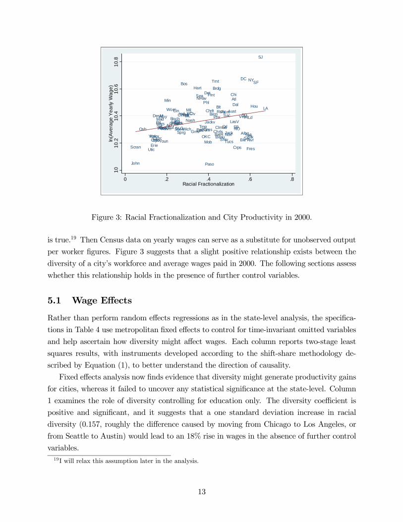
is true.19 Then Census data on yearly wages can serve as a substitute for unobserved output

per worker figures. Figure 3 suggests that a slight positive relationship exists between the

diversity of a city’s workforce and average wages paid in 2000. The following sections assess

whether this relationship holds in the presence of further control variables.

5.1 Wage Effects

Rather than perform random effects regressions as in the state-level analysis, the specifica-

tions in Table 4 use metropolitan fixed effects to control for time-invariant omitted variables

and help ascertain how diversity might affect wages. Each column reports two-stage least

squares results, with instruments developed according to the shift-share methodology de-

scribed by Equation (1), to better understand the direction of causality.

Fixed effects analysis now finds evidence that diversity might generate productivity gains

for cities, whereas it failed to uncover any statistical significance at the state-level. Column

1 examines the role of diversity controlling for education only. The diversity coefficient is

positive and significant, and it suggests that a one standard deviation increase in racial

diversity (0.157, roughly the difference caused by moving from Chicago to Los Angeles, or

from Seattle to Austin) would lead to an 18% rise in wages in the absence of further control

variables.19I will relax this assumption later in the analysis.

13

The large magnitude of this coefficient suggests that further controls are necessary. First,

many papers on metropolitan productivity emphasize the key role of population density in

fostering creativity and generating urbanization externalities and productivity spillovers.20

Column 2 accounts for employment density and potential urbanization spillovers by including

a term measuring hundreds of employees per square mile. The coefficient on density (0.058)

is positive and significant — an increase in 100 employees per square mile is associated with a

5.8% increase in wages. More interestingly, the magnitude of the diversity coefficient reduces

by about a third.

Density alone may be insufficient in controlling for city characteristics. For example, two

cities may be identical in density, but one could be growing and attracting people of different

races, while the other is decaying. If so, then diversity will be positively correlated with the

strength of a city, and its coefficient in Columns 1 and 2 will exhibit a positive bias. To

better account for a city’s health and the heterogenous macroeconomic shocks that correlate

with both wages and diversity, Column 3 includes the metropolitan area unemployment rate

as a proxy for city-specific economic performance. Its coefficient is insignificant (though it

exhibits a surprising positive correlation with wages in later regressions), and does not alter

the results for diversity.

Table 4: Racial Diversity and the Effect on Metropolitan Wages, a Proxy for Productivity.

1 2 3 4 5 6Diversity 1.156 0.796 0.781 0.699 0.225 0.383

(0.304)*** (0.291)*** (0.281)*** (0.258)*** (0.194) (0.150)**

Non-White Employment -0.006(0.004)

Years of Schooling 0.165 0.134 0.139 0.142 0.180 0.136(0.045)*** (0.047)*** (0.047)*** (0.049)*** (0.026)*** (0.044)***

Employment Density 0.058 0.057 0.064 0.011 0.023(0.024)** (0.024)** (0.023)*** (0.025) (0.024)

Unemployment Rate 0.006 0.009 0.009 0.013(0.005) (0.005)** (0.004)** (0.004)***

Public Employment -0.010 -0.006 -0.005(0.004)*** (0.003)** (0.003)

Average Rent 0.002 0.002(0.000)*** (0.000)***

Observations 309 309 309 309 309 309R-Squared 0.95 0.96 0.96 0.96 0.98 0.98

Panel covers 103 metropolitan areas in 1980, 1990, and 2000.Two-stage least squares (IV) with fixed effects.Diversity measured as racial fractionalization (RF) of employed labor force.Non-White and Public Employment measure the share of a state's employees who are not white and are working for government agencies, respectively.Employment Density measures hundreds of employees per square mile.Average Rent measures the average residential rental price per room in a city.Cluster-robust standard errors in parenthesis.*** Coefficient significant at 1%.** Coefficient significant at 5%.* Coefficient significant at 10%.Constant and decade indicator variables suppressed.

Dependent Variable: ln(Average Yearly Wage)

20See Harris and Ioannides (2000), Ciccone and Hall (1996), and Jacobs (1969).

14

Column 4 controls for public sector employment, since wages in this sector might not

be determined by market forces as the use of wages as a proxy for productivity assumes.

Inclusion of this variable does little to alter the marginal effect of diversity. The results

suggest that a one standard deviation increase in diversity still facilitates an 11% rise in

wages.

Some analysts argue that higher wages associated with diversity may simply reflect cost

of living differences across metropolitan areas that the employment density variable fails to

capture, and that regressions should control for this accordingly. Ottaviano and Peri (2005

and 2006), however, argue that unadjusted wages are indeed the appropriate proxy for pro-

ductivity, that cost of living differences establish the equilibrium number of workers in each

city, and that wage regressions should not include cost of living proxies among the explana-

tory variables. Though I am more sympathetic to Ottaviano and Peri’s arguments, Columns

5 and 6 include the average home rental price per dwelling room as a proxy for a city’s cost

of living for completeness.21 This causes the effects of diversity to drop substantially, even

losing statistical significance in Column 5.

One might suspect that an increase in diversity would lead to lower average wages paid

to workers since minorities do tend to earn lower wages than White workers earn. The final

specification in Table 4 accounts for this fact by including both racial fractionalization (as

a measure of diversity) and the Non-White share of employment (to control for lower wages

paid to minorities). This restores the positive and significant relationship between diversity

and wages. If the model’s assumptions are correct, a one standard deviation increase in

diversity causes average wages to rise roughly 6.0%.22

5.2 Wages and Employment

If diversity does not affect labor supply, then the wage regression results of the previous sub-

section imply that diversity causes city productivity to rise. If this assumption is untenable,

however, then macroeconomic wage regressions are insufficient in identifying the productiv-

ity effects of diversity. Glaeser, Scheinkman, and Shleifer (1995), for example, argue that

cross-city regressions should employ population size (or growth) as a proxy for productiv-

ity since labor mobility implies that individuals will move to high-income areas. Moreover,

economists since Becker (1971) have recognized the possible existence of a compensating

differential paid to White workers. That is, diversity could alter labor supply if Whites

are less willing to work with minorities. If true, then no instrument would be capable of

21This is the IPUMS variable RENT divided by ROOMS.22Appendix A.3 illustrates that the wage effects identified in this section do not vary across regions of the

United States.

15

identifying whether an increase in wages associated with diversity reflects productivity gains

or reduced labor supply. To robustly determine whether diversity augments productivity,

I now pursue a comparative statics exercise and consider simultaneous estimation of wages

and employment.23

Changes in equilibrium wages and employment together demonstrate the net effect of

supply and demand shifts. If diversity causes either employment or wages to rise, without

causing the other to fall, then diversity generated productivity gains. Conversely, if diversity

causes wages or employment to fall without causing the other to rise, diversity reduces

productivity. Ambiguous productivity implications occur only when diversity has opposite

effects on wages and employment.

The three-stage least squares specification in Equation (3), with instrumental variables

described in Section 3, can help ascertain the direction of diversity’s effect on productivity.

The wage equation replicates previous wage regressions that argued for the existence of pos-

itive gains from diversity. The innovation lies in the employment equation, which relates

a city’s employment to the same diversity and control variables of the wage equation. Im-

portantly, the dependent variable controls for size effects caused by employment growth at

the national level by dividing the size of each city’s employment by the total size of the US

workforce.24 Diversity is likely to increase productivity if the sign on fractionalization in ei-

ther the wage or employment regression is positive, and the sign in the other is non-negative.

Conversely, if the sign in one regression is negative and the other is non-positive, diversity

likely causes productivity to decrease.

ln(wc,t) = αw + βw ∗Divc,t +KXk=1

γw,k ∗ Controlk,c,t +2000X

t=1990

δw,t ∗Decc,t + c,t (3)

Empc,t = αl + βl ∗Divc,t +KXk=1

γl,k ∗ Controlk,c,t +2000X

t=1990

δl,t ∗Decc,t + c,t

Where c = 103 metropolitan areas, t = 3 decades.

w = Average yearly wage earnings of employees.

Emp = Employment share of total US employment.

Div = Diversity variable (racial fractionalization).

Control = Control variables 1 through K.

Dec = Decade indicator variables for 1990 and 2000.23Also see Ottaviano and Peri (2006) and Sparber (2007).24As with all other share variables, I record the employment share value in whole-number terms.

16

The first set of regressions in Table 5 control for the share of Non-White employment,

educational attainment, employment density, unemployment, the size of the public sector,

and the cost of living. One limitation of this specification, however, is that it includes a

measure of employment on both the left and right hand side of the specification. Column 2

compensates by dropping the density term. Column 3 also drops the cost of living variable,

given that the appropriateness of its inclusion is questionable. In all three specifications,

the results suggest that diversity causes average wages to rise. Furthermore, employment is

insensitive to changes in diversity. Thus, it appears that diversity-generated wage gains are

at least partly the consequence of productivity increases, not just changes in labor supply.

Table 5: Racial Diversity and its Effect on Wages and Employment.

Wage Emp Wage Emp Wage EmpDiversity 0.383 1.186 0.444 0.241 0.727 0.567

(0.119)*** (0.747) (0.114)*** (0.504) (0.151)*** (0.460)

Non-White Employment -0.006 -0.057 -0.007 -0.035 0.007 -0.019(0.003)** (0.017)*** (0.003)** (0.013)*** (0.003)*** (0.008)**

Years of Schooling 0.136 -0.328 0.141 -0.403 0.226 -0.305(0.026)*** (0.160)** (0.024)*** (0.107)*** (0.026)*** (0.080)***

Employment Density 0.023 -0.348(0.011)** (0.069)***

Unemployment Rate 0.013 0.050 0.014 0.035 0.005 0.026(0.003)*** (0.017)*** (0.003)*** (0.012)*** (0.003)* (0.010)***

Public Employment -0.005 -0.007 -0.004 -0.009 -0.014 -0.020(0.002)*** (0.010) (0.002)*** (0.007) (0.002)*** (0.006)***

Average Rent 0.002 0.009 0.003 0.003(0.000)*** (0.002)*** (0.000)*** (0.001)***

Constant 7.832 16.739 7.991 14.296 6.986 13.140(0.322)*** (2.024)*** (0.337)*** (1.482)*** (0.376)*** (1.146)***

Observations 309 309 309 309 309 309

Panel covers 103 metropolitan areas in 1980, 1990, and 2000.Three-stage least squares (IV) with fixed effects.Diversity measured as racial fractionalization (RF) of employed labor force.Non-White and Public Employment measure the share of a state's employees who are not white and are working for government agencies, respectively.Employment Density measures hundreds of employees per square mile.Average Rent measures the average residential rental price per room in a city.Standard errors in parenthesis.*** Coefficient significant at 1%.** Coefficient significant at 5%.* Coefficient significant at 10%.Decade indicator variables suppressed.

3

Dependent Variables: ln(Average Yearly Wage)

Employed Labor Force (Share of US Employed LF)

1 2

6 Conclusions

Racial diversity has risen dramatically in the United States during recent decades and will

continue to do so in the near future. International studies often find that diversity reduces

macroeconomic growth and productivity. However, other analyses suggest that diversity may

be capable of augmenting productivity. This paper analyzed the role of racial heterogeneity

within the US.

17

State-level regressions deliver mixed results. Fixed effects analysis fails to uncover any

causal connection between diversity and gross state output per worker. A robust Hausman

test supports a parsimonious random effects specification, however, which argues that a one

standard deviation increase in diversity raises productivity by roughly 5.9%.

Unlike for states, fixed effects analysis at the city-level is informative. A one standard

deviation diversity shock causes wages to rise by about 6.0% in regressions controlling for

many other wage determinants. Furthermore, three-stage least squares regressions demon-

strate that changes in labor supply cannot explain the entirety of this increase. Wage gains

appear to be due, at least in part, to productivity shifts.

The macroeconomic methodology in this paper explored whether cross-sectional evidence

within the United States suggests that diversity generates net economic gains or losses. It

did not evaluate the channels through which diversity affects productivity. These important

issues are probably best served by alternative methodologies, including those employing

experimental, behavioral, and micro-level data. Further research in these areas will provide

valuable added insight into the economic consequences of diversity.

18

References

[1] Adams, Terry K. (1992), Census of Population and Housing, 1970 [United States]:

Extract Data, Computer File. Courtesy of the Inter-University Consortium for Political

and Social Research, http://www.icpsr.umich.edu/, Study No. 9694.

[2] Alesina, Alberto, Reza Baqir, and William Easterly (1999), “Public Goods and Ethnic

Divisions,” Policy Research Working Paper Series 2108, The World Bank.

[3] Alesina, Alberto, Arnaud Devleeschauwer, William Easterly, Sergio Kurlat, and Romain

Wacziarg (2003), “Fractionalization,” Journal of Economic Growth, Vol. 8(2): 155-194.

[4] Alesina, Alberto and Edward L. Glaeser (2004), Fighting Poverty in the US and Europe.

New York: Oxford University Press.

[5] Alesina, Alberto and Elieana La Ferrara (2005), “Ethnic Diversity and Economic Per-

formance,” Journal of Economic Literature, Vol. 43(3): 762-800.

[6] Becker, Gary S. (1971), The Economics of Discrimination. Chicago: University of

Chicago Press.

[7] Bergman, Mike (2004), “More Diversity, Slower Growth,” US Census Bureau News,

http://www.Census.gov/population/www/documentation/twps0056.html.

[8] Brief of Amici Curiae Steelcase, Inc. et al., Gratz v. Bollinger, 135 F.Supp.2d 790 (2001)

(No. 97-75231).

[9] Card, David (2001), “Immigrant Inflows, Native Outflows, and the Local Labor Market

Impacts of Higher Immigration,” Journal of Labor Economics, Vol. 19: 22-61.

[10] Campbell, Donald. (1960), “Blind Variation and Selective Retention in Creative

Thought as in Other Knowledge Processes,” Psychological Review, Vol. 67: 380-400.

[11] Caselli, Francesco and John Coleman (2002), “On the Theory of Ethnic Conflict,” Work-

ing Paper, Harvard University.

[12] Ciccone, Antonio and Robert Hall (1996), “Productivity and the Density of Economic

Activity,” American Economic Review, Vol. 86(1): 54-70.

[13] Coleman, James S. (1988), “Social Capital in the Creation of Human Capital,”American

Journal of Sociology, Vol. 94(Supplement): S95-S120.

19

[14] Collier, Paul (2000), “Ethnicity, Politics, and Economic Performance,” Economics and

Politics, Vol. 12(3): 225-246.

[15] Collier, Paul (2001), “Implications of Ethnic Diversity,” Economic Policy: A European

Forum, Vol. 0(32): 127-155.

[16] Cox, Taylor H., Sharon A. Lobel, and Poppy Lauretta McLeod (1991), “Effects of Eth-

nic Group Cultural Differences on Cooperative and Competitive Behavior on a Group

Task,” Academy of Management Journal, Vol. 34(4): 827-847.

[17] Easterly, William and Ross Levine (1997), “Africa’s Growth Tragedy: Policies and

Ethnic Divisions,” The Quarterly Journal of Economics, Vol. 112(4): 1203-1250.

[18] Fearon, James D. (2003), “Ethnic and Cultural Diversity by Country,” Journal of Eco-

nomic Growth, Vol. 8(2): 195-222.

[19] Florida, Richard (2002), The Rise of the Creative Class. New York: Basic Books.

[20] Fukuyama, Francis (1999), “Social Capital and Civil Society,” Prepared for the IMF

Conference on Second Generation Reforms.

[21] Garofalo, Gasper A. and Steven Yamarik (2002), “Regional Convergence: Evidence from

a New State-by-State Capital Stock Series,” The Review of Economics and Statistics,

Vol. 84(2): 316-323.

[22] Gibson, Campbell and Kay Jung (2002), “Historical Census Statistics on Population To-

tals by Race, 1790 to 1990, and by Hispanic Origin, 1970 to 1990, for the United States,

Regions, Divisions, and States,” Working Paper Series No. 56, Population Division, US

Census Bureau.

[23] Gilens, Martin (1999), Why Americans Hate Welfare. Chicago: The University of

Chicago Press.

[24] Glaeser, Edward L., Jose A. Scheinkman, and Andrei Shleifer (1995), “Economic Growth

in a Cross-Section of Cities,” Journal of Monetary Economics, Vol. 36(1): 117-143.

[25] Greif, Avner (1993), “Contract Enforceability and Economic Institutions in Early Trade:

The Maghribi Traders Coalition,” American Economic Review, Vol. 83(3): 525-548.

[26] Hall, Robert and Charles I. Jones (1999), “Why do Some Countries Produce So Much

More Output Per Worker Than Others?” The Quarterly Journal of Economics, Vol.

114(1): 83-116.

20

[27] Hamilton, Barton H., Jack A. Nickerson, and Hideo Owan (2003), “Team Incentives and

Worker Heterogeneity: An Empirical Analysis of the Impact of Teams on Productivity

and Participation,” Journal of Political Economy, Vol. 111(3): 465-497.

[28] Harris, Timothy F. and Yannis Ioannides (2000), “Productivity and Metropolitan Den-

sity,” No 16, Discussion Paper Series, Department of Economics, Tufts University.

[29] Hellerstein, Judith and David Neumark (2004), “Production Function and Wage Equa-

tion Estimation with Heterogeneous Labor: Evidence from a New Matched Employer-

Employee Data Set,” NBER Working Paper No. 10325.

[30] Hong, Lu and Scott E. Page (2004), “Groups of Diverse Problem Solvers Can Outper-

form Groups of High-Ability Problem Solvers,” Proceedings of the National Academy,

Vol. 101(46): 16385-16389.

[31] Jacobs, Jane (1969), The Economy of Cities. New York: Random House.

[32] Knack, Stephen and Philip Keefer (1997), “Does Social Capital Have an Economic

Payoff? A Cross-Country Investigation,” The Quarterly Journal of Economics, Vol.

112(4): 1251-1273.

[33] Luttmer, Erzo F.P. (2001), “Group Loyalty and the Taste for Redistribution,” Journal

of Political Economy 109(3): 500-528.

[34] Mauro, Paolo (1995), “Corruption and Growth,” The Quarterly Journal of Economics,

Vol. 110(3): 681-712.

[35] Mincer, Jacob (1974), Schooling, Experience, and Earnings. New York: Columbia Uni-

versity Press.

[36] National Bureau of Economic Research (2004), CPS Merged Outgoing Rotation Groups.

CD-ROM available at http://www.nber.org/data/morg.html.

[37] National Research Council (2004), Measuring Racial Discrimination. Panel on Methods

for Assessing Discrimination, Rebecca M. Blank, Marilyn Dabady, and Constance F.

Citro, Editors. Committee on National Statistics, Division of Behavioral and Social

Sciences and Education. Washington, DC: The National Academies Press.

[38] Neal, Derek and William Johnson (1996), “The Role of Premarket Factors in Black-

White Wage Differences,” Journal of Political Economy 104(5): 869-895.

[39] Neumark, David (1998), “Labor Market Information,” NBERWorking Paper No. 6573.

21

[40] O’Reilly, Charles A. III, Katherine Y. Williams, and Sigal Barsade (1998), “Group

Demography and Innovation: Does Diversity Help?,” Research on Managing Groups

and Teams, Vol. 1: 183-297.

[41] Ottaviano, Gianmarco I.P., and Giovanni Peri (2005), “Cities and Cultures,” Journal

of Urban Economics, Vol. 58(2): 304-337.

[42] Ottaviano, Gianmarco I.P., and Giovanni Peri (2006), “The Economic Value of Cultural

Diversity: Evidence from US Cities,” Journal of Economic Geography, Vol. 6(1): 9-44.

[43] Page, Scott E. (2007), The Difference — How the Power of Diversity Creates Better

Groups, Firms, Schools, and Societies. Princeton, NJ: Princeton University Press.

[44] Posner, Daniel N. (2004), “Measuring Ethnic Fractionalization in Africa,” American

Journal of Political Science, Vol. 48(4): 849-863.

[45] Poterba, James M. (1997), “Demographic Structure and the Political Economy of Public

Education,” Journal of Policy Analysis and Management, Vol. 16(1): 48-66.

[46] Psacharopoulos, George (1994), “Returns to Investment in Education: A Global Up-

date,” World Development, 22(9): 1325-1343.

[47] Putnam, Robert D. (2007), “E Pluribus Unum: Diversity and Community in the

Twenty-first Century. The 2006 Johan Skytte Prize Lecture,” Scandinavian Political

Studies, Vol. 30(2): 137-174.

[48] Ruggles, Steven, Matthew Sobek, Trent Alexander, Catherine A. Fitch, Ronald Goeken,

Patricia Kelly Hall, Miriam King, and Chad Ronnander. Integrated Public Use Micro-

data Series: Version 3.0 [Machine-readable database]. Minneapolis, MN: Minnesota

Population Center [producer and distributor], 2004. http://www.ipums.org.

[49] Simonton, Dean Keith (1999), Origins of Genius, Darwinian Perspectives on Creativity.

New York: Oxford University Press.

[50] Sparber, Chad (2007), “Racial Diversity and Aggregate Productivity in US Industries:

1980-2000,” Working Paper, Colgate University.

[51] U.S. Dept. of Commerce, Bureau of the Census (198?), Census of Population and Hous-

ing, 1980: Summary Tape File 3B, Computer File. Courtesy of the Inter-University

Consortium for Political and Social Research, http://www.icpsr.umich.edu/, Study No.

8318.

22

[52] U.S. Dept. of Commerce, Bureau of the Census (1982), Current Population Survey, May

1980. Available at http://www.nber.org/data/cps_may.html.

[53] U.S. Dept. of Commerce, Bureau of the Census (1993), Census of Population and Hous-

ing, 1990: Summary Tape File 3B, Computer File. Courtesy of the Inter-University

Consortium for Political and Social Research, http://www.icpsr.umich.edu/, Study No.

6116.

[54] U.S. Dept. of Commerce, Bureau of the Census (2000), Census of Population and Hous-

ing, 2000: Summary File 1. “Table GCT-PH1 Population Housing Units, Area, and

Density: 2000 Geography.”

[55] U.S. Dept. of Commerce, Bureau of the Census (2000), Census of Population and Hous-

ing, 2000: Summary File 3. DVD-ROM.

[56] U.S. Dept. of Commerce, Bureau of the Census (2004), International Data Base, Table

094, http://www.Census.gov/ipc/www.idbprint.html.

[57] U.S. Dept. of Commerce, Bureau of the Census (2006), Current Population Survey,

Merged Outgoing Rotation Groups. Available at http://www.nber.org/data/morg.html.

[58] U.S. Dept. of Commerce, Bureau of Economic Analysis (2004), Gross State Product.

http://www.bea.doc.gov/bea/regional/gsp/.

23

A Appendix

A.1 Metropolitan Regions in City-Level Regressions

The city-level regressions in Section 5 include only the metropolitan areas for which racial

composition data is available in 1970, 1980, 1990, and 2000. IPUMS provides this data for

the 103 metropolitan areas in Table 6.

Table 6: Metropolitan Areas Considered in City-Level Analysis.Akron, OH Milwaukee, WIAlbany-Schenectady-Troy, NY Minneapolis-St. Paul, MNAlbuquerque, NM Mobile, ALAllentown-Bethlehem-Easton, PA/NJ Nashville, TNAppleton-Oskosh-Neenah, WI New Haven-Meriden, CTAtlanta, GA New Orleans, LAAustin, TX New York-Northeastern NJBakersfield, CA Norfolk-VA Beach--Newport News, VABaltimore, MD Oklahoma City, OKBaton Rouge, LA Orlando, FLBeaumont-Port Arthur-Orange,TX Peoria, ILBirmingham, AL Philadelphia, PA/NJBoston, MA-NH Phoenix, AZBridgeport, CT Pittsburgh, PABuffalo-Niagara Falls, NY Portland, OR-WACanton, OH Providence-Fall River-Pawtucket, MA/RICharleston-N.Charleston,SC Reading, PACharlotte-Gastonia-Rock Hill, NC-SC Richmond-Petersburg, VAChicago, IL Riverside-San Bernadino, CACincinnati-Hamilton, OH/KY/IN Rochester, NYCleveland-Lorain-Elyria, OH Rockford, ILColumbia, SC Sacramento, CAColumbus, OH St. Louis, MO-ILCorpus Christi, TX Salinas-Sea Side-Monterey, CADallas-Fort Worth, TX Salt Lake City-Ogden, UTDayton-Springfield, OH San Antonio, TXDes Moines, IA San Diego, CADetroit, MI San Francisco-Oakland-Vallejo, CAEl Paso, TX San Jose, CAErie, PA Santa Barbara-Santa Maria-Lompoc, CAFlint, MI Scranton-Wilkes-Barre, PAFort Lauderdale-Hollywood-Pompano Beach, FL Seattle-Everett, WAFort Wayne, IN Shreveport, LAFresno, CA South Bend-Mishawaka, INGrand Rapids-Muskegon, MI Spokane, WAGreensboro-Winston Salem-High Point, NC Springfield-Holyoke-Chicopee, MAGreenville-Spartanburg-Anderson SC Stockton, CAHarrisburg-Lebanon--Carlisle, PA Syracuse, NYHartford-Bristol-Middleton- New Britain, CT Tacoma, WAHouston-Brazoria, TX Tampa-St. Petersburg-Clearwater, FLIndianapolis, IN Trenton, NJJackson, MS Tucson, AZJacksonville, FL Tulsa, OKJohnstown, PA Utica-Rome, NYKansas City, MO-KS Ventura-Oxnard-Simi Valley, CAKnoxville, TN Washington, DC/MD/VALancaster, PA West Palm Beach-Boca Raton-Delray Beach, FLLansing-E. Lansing, MI Wichita, KSLas Vegas, NV Worcester, MALittle Rock--North Little Rock, AR York, PALos Angeles-Long Beach, CA Youngstown-Warren, OH-PAMadison, WI

24

A.2 Alternative State-Level Regressions

The regression specification in Equation (2) is missing a clear determinant of labor pro-

ductivity — capital per worker. Many growth economists resist introducing capital stock

measures directly into labor productivity regressions since capital is highly correlated with

omitted variables in the error term. If true, then estimation of the coefficient will have a

large upward bias. One solution is to instead follow a growth accounting procedure.

Suppose Equation (4) describes how output per worker (y) is determined by physical

and human capital per worker (k and h, respectively) and a total factor productivity term

(TFP ) complementing these factors of production.

y = TFP · kα · h1−α (4)

Total factor productivity can only be measured after employing a number of assumptions.

Hall and Jones (1999) propose a production function similar to (4). They appeal to economic

theory and assume that α equals the percentage of income earned by capital (roughly 1/3).

To ascertain values of h, they turn to evidence on the rate of return to education from

Mincer (1974) and Psacharopoulos (1994) that suggests h = exp (0.94 + 0.068 · (t− 8)),where t measures the average number of years of schooling. By substituting this expression

into (4), taking the natural logarithm of both sides, and rearranging, the level of TFP in an

economy then equals the identity in Equation (5).

ln (TFP ) = ln(y)−µ1

3

¶ln (k)−

µ2

3

¶(0.94 + 0.068 · (t− 8)) (5)

Suppose diversity affects labor productivity (y) through total factor productivity (TFP ).

To test this possibility, I first construct TFP estimates for states by using BEA gross state

output data, education data from IPUMS, capital stock figures developed according to the

methodology created by Garofalo and Yamarik (2002), and the identity in Equation (5).

Then I perform two-stage least squares regressions, with instruments described in Section 3,

according to the specification in Equation (6). The regression methodology is analogous to

that in Section 4.

25

ln(TFPs,t) = α+ β ∗Divs,t +2000X

t=1990

δt ∗Decades,t + s,t (6)

Where s = 48 contiguous states, t = 3 decades.

TFP = Total factor productivity.

Div = Diversity variable (racial fractionalization).

Decade = Decade indicator variables for 1990 and 2000.

= Error term.

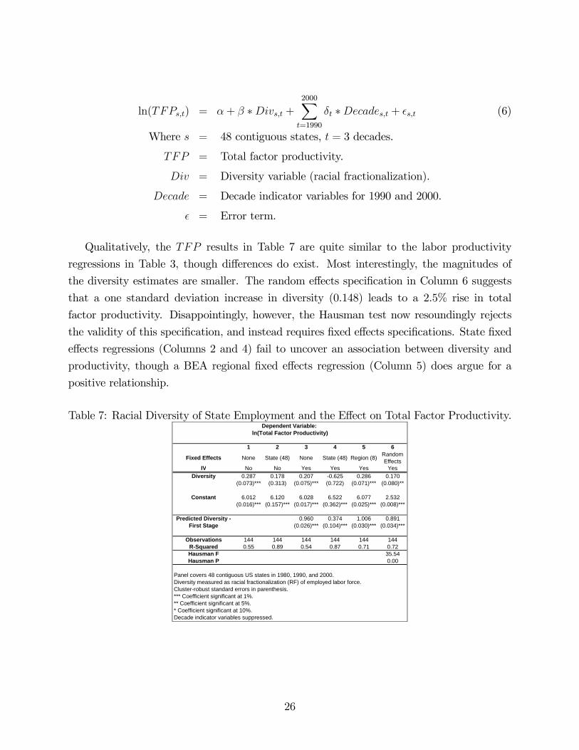
Qualitatively, the TFP results in Table 7 are quite similar to the labor productivity

regressions in Table 3, though differences do exist. Most interestingly, the magnitudes of

the diversity estimates are smaller. The random effects specification in Column 6 suggests

that a one standard deviation increase in diversity (0.148) leads to a 2.5% rise in total

factor productivity. Disappointingly, however, the Hausman test now resoundingly rejects

the validity of this specification, and instead requires fixed effects specifications. State fixed

effects regressions (Columns 2 and 4) fail to uncover an association between diversity and

productivity, though a BEA regional fixed effects regression (Column 5) does argue for a

positive relationship.

Table 7: Racial Diversity of State Employment and the Effect on Total Factor Productivity.

1 2 3 4 5 6

Fixed Effects None State (48) None State (48) Region (8) Random Effects

IV No No Yes Yes Yes YesDiversity 0.287 0.178 0.207 -0.625 0.286 0.170

(0.073)*** (0.313) (0.075)*** (0.722) (0.071)*** (0.080)**

Constant 6.012 6.120 6.028 6.522 6.077 2.532(0.016)*** (0.157)*** (0.017)*** (0.362)*** (0.025)*** (0.008)***

Predicted Diversity - 0.960 0.374 1.006 0.891First Stage (0.026)*** (0.104)*** (0.030)*** (0.034)***

Observations 144 144 144 144 144 144R-Squared 0.55 0.89 0.54 0.87 0.71 0.72Hausman F 35.54Hausman P 0.00

Panel covers 48 contiguous US states in 1980, 1990, and 2000.Diversity measured as racial fractionalization (RF) of employed labor force.Cluster-robust standard errors in parenthesis.*** Coefficient significant at 1%.** Coefficient significant at 5%.* Coefficient significant at 10%.Decade indicator variables suppressed.

Dependent Variable: ln(Total Factor Productivity)

26

A.3 Region-Specific Effects of Diversity

Diversity may possibly affect some regions more than others. One obvious scenario worth

exploring is whether diversity has a different effect within border states and former states

of the confederacy, given the high rates of diversity in those states due to geographical

and historical factors. Columns 1, 2, and 3 of Table 8 test this possibility by altering

the specifications in Columns 1, 4, and 5 of Table 4, respectively. The final column assesses

whether the West Coast’s proximity to Asia might also lead to a differential effect of diversity.

Despite the intuitive argument that differential effects might exist, evidence suggests that

the effects are quite similar across regions.

Table 8: Racial Diversity and the Effect on Metropolitan Wages within Regions.

1 2 3 4Diversity 0.894 0.417 0.312 0.373

(0.314)*** (0.245)* (0.191) (0.197)*

Diversity * Confederate 0.158 -0.014 0.050 0.002(0.246) (0.196) (0.158) (0.155)

Diversity * Border 0.438 0.322 0.207 0.249(0.215)** (0.275) (0.239) (0.218)

Diversity * West -0.193(0.139)

Non-White Employment 0.003 0.141 -0.007(0.006) (0.048)*** (0.006)

Years of Schooling 0.204 0.193 0.029 0.138(0.048)*** (0.051)*** (0.027) (0.045)***

Employment Density 0.057 -0.007 0.025(0.029)** (0.005) (0.027)

Unemployment Rate 0.008 0.013 0.012(0.007) (0.006)** (0.006)**

Public Employment -0.010 -0.004 -0.004(0.004)** (0.004) (0.004)

Average Rent 0.002 0.002(0.001)*** (0.000)***

Observations 309 309 309 309R-Squared 0.95 0.97 0.98 0.98

Panel covers 103 metropolitan areas in 1980, 1990, and 2000.Two-stage least squares (IV) with fixed effects.Diversity measured as racial fractionalization (RF) of employed labor force.Non-White and Public Employment measure the share of a state's employees who are not white and are working for government agencies, respectively.Employment Density measures hundreds of employees per square mile.Average Rent measures the average residential rental price per room in a city.Confederate, Border, and West are indicator variables for former members of the Confederacy, states that share a border with Mexico, and West Coast states, respectively.Cluster-robust standard errors in parenthesis.*** Coefficient significant at 1%.** Coefficient significant at 5%.* Coefficient significant at 10%.Constant and decade indicator variables suppressed.

Dependent Variable: ln(Average Yearly Wage)

27