how race and religion shape millennial attitudes on sexuality and ...
Race, Religion and the City: Twitter Word Frequency Patterns
Reveal Dominant Demographic Dimensions in the United States
Eszter Bokanyi∗1, Daniel Kondor1,2, Laszlo Dobos1, Tamas Sebok1, Jozsef Steger1,Istvan Csabai1, and Gabor Vattay1
1Department of Physics of Complex Systems, Eotvos Lorand University, Pazmany Peter setany 1/A, H-1117Budapest, Hungary
2SENSEable City Laboratory, Massachusetts Institute of Technology, 77 Massachusetts Avenue, Cambridge, MA02139, USA
Abstract
Recently, numerous approaches have emerged in the social sciences to exploit the opportunitiesmade possible by the vast amounts of data generated by online social networks (OSNs). Havingaccess to information about users on such a scale opens up a range of possibilities – from predictingindividuals’ demographics and health status to their beliefs and political opinions – all without thelimitations associated with often slow and expensive paper-based polls. A question that remainsto be satisfactorily addressed, however, is how demography is represented in the OSN content –that is, what are the relevant aspects that constitute detectable large-scale patterns in language?Here, we study language use in the US using a corpus of text compiled from over half a billiongeo-tagged messages from the online microblogging platform Twitter. Our intention is to revealthe most important spatial patterns in language use in an unsupervised manner and relate them todemographics. Our approach is based on Latent Semantic Analysis (LSA) augmented with the RobustPrincipal Component Analysis (RPCA) methodology, which permits identification of the data’s mainsources of variation with an automatic filtering of noise and outliers without influencing results bya priori assumptions. We find spatially correlated patterns that can be interpreted based on thewords associated with them. The main language features can be related to slang use, urbanization,travel, religion and ethnicity, the patterns of which are shown to correlate plausibly with traditionalcensus data. Apart from the standard measure of linear correlation, some relations seem to be betterexplained by boolean implications, suggesting a threshold-like behavior where demographic variablesinfluence the users’ word use. Our findings thus validate the concept of demography being representedin OSN language use and show that the traits observed are inherently present in the word frequencieswithout any previous assumptions about the dataset. Thus, they could form the basis of furtherresearch focusing on the evaluation of demographic data estimation from other big data sources, oron the dynamical processes that result in the patterns found here.
1 Introduction
Geography plays an important role in many social phenomena: clearly, many aspects of life are influencedby the possibilities offered by the environment in which one lives [1–6]. As such, uncovering the spatialstructures and the dynamics of changes in them has for some time been a focus of the scientific commu-nity and policymakers. In line with this, governments and local authorities invest significant resourcesin creating and maintaining databases of census data, including several variables describing the localpopulation and economic activity on the regional scale. These data-collection and monitoring activitiesare usually limited by the significant efforts required to obtain and process data, prompting researchersand professionals to look for alternative data sources and methods that can complement traditional datacollection and which could be integrated with modeling and research efforts [7–13].
In the past two decades, there has been a significant growth in the amount of data collected aboutindividuals that has been made available for research purposes. This has had a large impact on socialscience research where empirical studies were previously limited by the cost and effort associated withdata collection. This includes studies focusing on how modern data collection methods can be used toreveal the spatial structure in society on several scales, and how quantities measured in the online or
1
arX
iv:1
605.
0295
1v1
[ph
ysic
s.so
c-ph
] 1
0 M
ay 2
016
abstract environments are connected to real-world phenomena. Two common data sources are mobilephone networks, where user activity and aggregated measures of network utilization are recorded atthe antenna level as part of regular operation [14] and online social networks (OSNs) [15], where thecontent publicly shared by users in many cases includes their position [16]. Some other data sources withpromising application possibilities include monetary transactions [17–19], GPS traces from cars [20, 21]and other devices and public transportation usage as recorded by electronic payment systems [22, 23].
Using these data, previous research has shown that it is possible to obtain accurate and up-to-datemeasures of population density [9] or crowd size at sports events or in airports [10]. Furthermore, thedemographic features of a city or a country can be estimated by parsing OSN user names or user profiledescriptions [24, 25]. By focusing on the community structure instead of estimating features of individuals,networks of connections among mobile phone or social network users reveal geographic clustering on largescales [18, 26, 27], Twitter users’ language choice reflects different cultural communities [28], while useractivity has been used on urban scales as an innovative method of land use detection [13, 29, 12, 11]. Inaddition to land use data, commuting and mobility patterns in the city [30, 31] and larger scale traveltrends can also be investigated with the help of mobile and OSN networks [32–34].
Apart from looking at the spatio-temporal patterns, analysing the content of users posted in OSNscan provide further insights, adapting text mining methods and results which have been previouslydeveloped and obtained on the growing corpus of digital texts [35–39]. From predicting heart-diseaserates of an area based on its language use [40], connecting health measures to photo scenicness ratings[41] or relating unemployment to social media content [42, 43] to forecasting stock market moves fromsearch semantics [44], many studies have attempted to connect online media language and metadata toreal-world outcomes. Various studies have analyzed spatial variation in the OSN messages’ texts andits applicability to several different questions, including user localization based on the content of theirposts [45, 46], empirical analysis of the geographic diffusion of novel words, phrases, trends and topics ofinterest [47, 48], measuring public mood [49].
In these studies, either a priori models were used, or a model was built with a supervised learningmethod, with a focus on the specific phenomenon, meaning the exploitation of only one aspect (username, user profile description, misspelled words, words connected to fatigue etc.), yet possibly neglectingthe dataset’s other features. While being effective, there remain the following questions: (a) what aremain patterns in the data in general; (b) can they be discovered without making a priori assumptionsabout what to look for; (c) can we relate these patterns to relevant real social phenomena.
In this study our goal is to analyze in an unsupervised manner how and to what extent regional-scaledemographic attributes are represented in social media posts. We approach this using geo-tagged shortmessages (tweets) posted on the Twitter microblogging service as a source of large-scale digital corpus.We employ a combination of Latent Semantic Analysis (LSA) [36] and Robust Principal ComponentAnalysis (RPCA) [50, 51], which permits us the automated identification of the most significant topicsand language use features with regional variation on Twitter. We use tweets posted in the USA over a3-year period aggregated at the county-level. This allows comparison with census data at the same level,thus allowing us to draw some hypotheses about the driving forces behind regional language dissimilaritypatterns.
2 Methods
2.1 Twitter dataset
We use the datastream freely provided by Twitter through their Application Program Interface (API),which amounts to approximately 1% of all sent messages. In this study, we focus on the part of thedatastream with geolocation information. These geolocated tweets originate from users who chose to allowtheir mobile phones to post the GPS coordinates along with a Twitter message. The total geolocatedcontent was found to only comprise a small percentage of all tweets; therefore with data collection focusingonly on these, a large fraction of all geo-tagged tweets can be gained [52].
Our dataset includes a total of 335 million tweets from the contiguous United Stated of Americacollected between February 2012 and June 2013. These are all geotagged – that is, they have GPScoordinates associated with them. We construct a geographically indexed database of these tweets,permitting the efficient analysis of regional features [53]. Using the Hierarchical Triangular Mesh (HTM)scheme for practical geographic indexing [54, 55], we assigned a US county to each tweet. County bordersare obtained from the GAdm database 1.
1http://gadm.org
2

2.2 Latent Semantic Indexing and Robust Principal Component Analysis
We aim to use a type of vector space model on our Twitter corpus, where documents correspond tocounty-level aggregated tweets. The terms we consider are raw words obtained after a tokenizationprocess, - that is, we apply a ’word-bag’ approach to our documents, effectively limiting any analysis toword frequencies and ignoring relations among words and longer phrases. We filter stop-words in severallanguages (most important being English and Spanish) to remove most common but uninformative termsfrom our data.
We construct a term-document matrix Wij as the as the number of occurrences of the i-th word in thej-th cell. As the population density of the USA is very heterogeneous, the number of word occurrencesin each county is also heterogeneous. To improve the quality of the dataset, we only include counties tcontain at least 10000 occurrences of at least 500 individual words. We also limit the words used to thosewith at least 10000 occurrences in at least 1000 individual counties. This way there remain 2800 countiesand 10132 words, which form the Wij word occurrence matrix. We normalize Wij so that the elementsare the relative frequencies of words in each county: Xij ≡Wij/
∑kWkj , i.e. we normalize each element
by the total number of words posted in that county; this is called inverse document frequency weighingin text-mining literature.
To identify all possible regional characteristics of language usage, we rely on techniques known fromthe field of natural language processing. There exist many feature or topic extraction methods, all ofthem aiming to reduce the dimensionality of the data by finding related or similar words and documents.A common approach is Latent Semantic Analysis (LSA) [36, 56], which applies Singular Vector Decom-position (SVD) on a word by document matrix derived from the corpus. This method groups wordstogether based on their semantic similarity [35], creating ’feature’ documents, of which the first few rep-resent the concepts causing the most variation in the data. A notable achievement of LSA is that it isan unsupervised learning method, thus providing information about the corpus without using a prioriassumptions or any arbitrary preselections based on the purpose of the examination.
According to the nature of our dataset, there are several users who generate automated messageslike weather stations, advertisers or tornado and earthquake advisories, which are considered as noise inour investigations. Especially in sparsely inhabited areas, these outlier messages can account for a largefraction of the dataset. Also, highly localized features, such as tourist attractions, can generate outliersof significant volume. This can result in highly localized outliers dominating the results of the SVD,making identifying relevant structure challenging. Applying the Robust PCA method [51, 50] allows usto preprocess the matrix before further analysis by separating it into a low-rank and a sparse part, whoseprincipal components can then be computed and analyzed separately. This means that the original datamatrix is written as a sum of two parts:
X = XS +XLR , (1)
where XS is a sparse matrix and XLR contains the dense but low-rank part of the data. The mathematicalcondition for finding XS and XLR is minimizing the sum
λ‖XS‖1 + ‖XLR‖σ , (2)
where for a matrix X of dimensions n1 × n2 with n1 ≥ n2, λ ≡ 1/√n1, and the norms are the l1 and
nuclear norms respectively:
‖X‖1 =∑ij
|Xij |
‖X‖σ =∑i
σi(X) .(3)
Here σi(X) denotes the i-th singular value of X. An efficient algorithm for finding XS and XLR is theinexact augmented Lagrangian method [50] (Matlab code developed by the authors of [50] implementingthe algorithm is publicly available 2). Employing this method results in the sparse part containing mostof the outliers, and and in true language use variations to be represented in the low-rank part. Due tothe structure of our data matrix, and the employed Robust PCA method, we choose not to subtractaverages from the data; of course, this will probably result in average word frequencies dominating thefirst principal component. We further analyze only the results of the LSA of the low-rank component.
2http://perception.csl.illinois.edu/matrix-rank/sample_code.html
3
2.3 Demographic data
To discover possible governing factors of the geographical language variation patterns and connectionsbetween topics and their geography, we correlate right singular vectors with a variety of demographic dataseries from the 2010 US Census 3, 2011 American Community Survey (ACS) 5 year estimates concerningeducational attainment by counties 4, county business patterns according to North American IndustryClassification System (NAICS) classification 5 and church adherence rates and congregations numbersper county provided by the the Association of Religion Data Archives (ARDA) 6.
2.4 Boolean relationship detection
Apart from evaluating linear correlation measures with the singular vectors, we also carry out a booleanrelationship detection, using the methodology of Sahoo et al. [57], which is based on calculating a teststatistic based on the contingency table of the scatterplots (e.g. Fig. 3f-j, see the next section for aninterpretation of the results displayed) after creating the four segments of the data with a horizontaland a vertical limit. We find the most significantly sparse segment by setting the limits so that the teststatistic gives a maximum for the specific segment. During the calculations, we set an error bar on bothside of the limits, and points being in this error zone are not taken into consideration when testing forthe sparseness.
If the contingency table is
A low A high ΣB low m00 m01 b0B high m10 m11 b1
Σ a0 a1 s
The test statistic for the four segments is
δ =mij − 〈mij〉√〈mij〉
,
where 〈mij〉 denotes the expected value in case of independent variables
〈mij〉 =ais
bjs· s.
If there are some points left in the segment, they are considered as an error, and the measure of errorwould be
ε =1
2
(mij
mi0 −mi1+mij
ai
).
We consider a segment significantly sparse if δ > 3, and ε < 0.2.Then in the whole range of variables A and B (using 100 steps in both directions and an error
boundary of 1,5% for the skipping of points near the borders) we measure δ and ε values, and take thesegmentation with the maximum δ for the sparse areas, where ε is still low enough.
3 Results
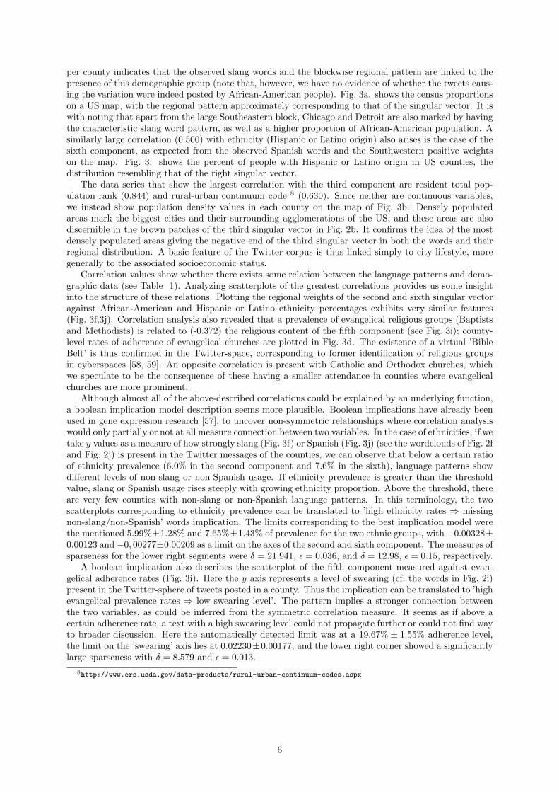
Using a corpus of over 335 million geo-tagged tweets posted in the USA, we compile word-frequencydistributions for each US county, and then apply the automatic filtering and feature selection methoddescribed. We analyze the features found with this technique by considering the connection betweengeographic and semantic distances (Fig. 1.), and by plotting right singular vectors on the map (Fig.2a-e.) and displaying left singular vectors as wordclouds (positive weights Fig. 2f-j., negative weightsFig. 2k-o.).
First, we find that the method applied successfully uncovers some coherent topics, especially in thefirst few singular vectors, where singular values are still great enough for the topic to give a significant
3http://www2.census.gov/census_2010/, http://www.census.gov/support/USACdataDownloads.html4http://www.census.gov/programs-surveys/acs/5http://www.census.gov/econ/cbp/6http://www.thearda.com
4

variance of the dataset. As we deliberately choose not to subtract averages from the Xij matrix, thefirst component shows no discernible pattern, and corresponds to the most common words in the sample.From the second singular vector, however, one or both ends (it can be either negative or positive, assingular vectors can arbitrarily be multiplicated by a minus sign) of each of the most important semanticfeatures on the wordclouds can be related to a certain language style, concept or lifestyle.
The words giving the largest contribution to the pattern of the second left singular vector (Fig. 2f.)mark a strong presence of slang in the sample. This includes forms with alternate spelling like ’aint’,’gotta’; swearing like ’ass’, ’hoe’, ’bitch’; abbreviations of common phrases like ’tryna’, ’imma’, ’kno’,’yall’; OSN-specific slang such as ’oomf’ which stands for ’one of my followers’ (i.e. on Twitter); avery specific misspelling of ’goodmorning’ (instead of ’good morning’); and variations of the racial slurs’nigga’ and ’niggas’. Swear words and abbreviations typical for online language also dominate this endof the component. The next most important feature, which can be found in the third vector (Fig. 2l.),identifies words connected to urban lifestyle like eating out (’pizza’, ’grill’), drinking coffee (’coffee’, ’cafe’,’starbucks’), education (’university’, ’library’, ’campus’) or working out (’gym’, ’fitness’).
Further dominating concepts are travel (’enjoying’, ’trip’, ’pic’, ’hotel’) in the fourth singular vector(Fig. 2h.) and religion (’lord’, ’prayers’, ’praying’, ’blessed’) alongside with positive content (’glad’,’thankful’, ’wonderful’, ’proud’) in the negatively weighed words of the fifth singular vector (Fig. 2n.). Inthis case, the opposite end can also be easily interpreted: the faith-related words in the fifth componentare countered by an increased usage of profanity present among words with positive weights (Fig. 2i.).This might be the consequence of people tweeting about religious topics also trying to avoid swearing;this hypothesis can also be supported with less strong swearing alternatives (’crap’, ’freaking’, ’dang’)prevailing among the negatively weighed words along the religious words.
If the native language of a group is different from that of the majority, the words of this differentlanguage also stand out from the overall structure, as there is naturally a stronger correlation amongwords belonging to the same language. Therefore the applied method can discover languages differentfrom that of the bulk of the sample. In the sixth singular vector, we can observe this phenomenon withSpanish words, which form more than the third of the positively weighed wordcloud (Fig. 2j.). TheEnglish terms ’Mexico’ and ’Mexican’ also appear in this group, which shows that concepts related tothe topic are also identified even if they do not belong to the discovered language.
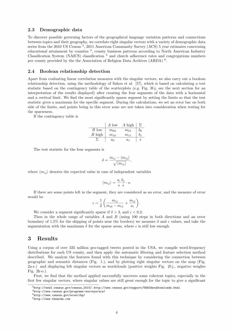
Similarly to topic identification, where semantically close words form topics, analyzing regional pat-terns reveal documents that are close to each other in the semantic space spanned by these topics. Plottingthe right singular vectors on a map (Fig. 2a-e.), the most striking feature is the regional proximity ofdocuments having close weights in the singular vectors. Document-by-document (county-by-county) Eu-clidean distances in the PCA subspace of the first 25 component as the function of real county-by-countycentroid distances 7 illustrate this observation. In Fig. 1. mean PCA subspace distances (red dots) areplotted for each 40 km range of real county centroid distances. As a baseline, the same is done for arandom permutation of counties (blue dots). It is remarkable that below 500 km, counties are closer inthe semantic space, as could be expected from a random realization. From 700 km to 1800 km, semanticdistance is greater than it would be randomly. Geographical proximity is thus a main driving force inthe similarity of language patterns in Twitter-space.
Analyzing these geographical patterns in each singular vectors provides insights into the regionaldistribution of the single topics. On a US map, the second component (Fig. 2a.), which is responsiblefor the most variance in the Twitter data, emerges as a block in the Southeastern part of the US.Apart from the big Southeastern block, Chicago and Detroit are also marked by this pattern of languageusage. In the third component (Fig. 2b.), negative weights (brown patches) mark the biggest citiesand surrounding counties which belong to their agglomeration. The most positive pattern of the fourthcomponent (Fig. 2c.) reveals some important touristic attractions such as the center of New York,Washington and San Francisco, the Craters of the Moon National Monument and Preserve in Idaho, AspenMountain ski area in Colorado or Hawaii. The regional pattern of the fifth component (Fig. 2d.) is lessobvious, though a part of the central US and the Southeastern block is discernible in the religion-relatedend of the component. The sixth component distinguishes the Southwestern part and the Northwesterncorner of the US (Fig. 2e.), Florida and some bigger cities such as New York or Chicago.
To discover possible governing factors of the geographical language variation patterns and their re-lation to demography, we calculate Pearson correlation values between right singular vectors and dataobtained from the US Census Bureau described in Section 2.3. Data series that have the greatest abso-lute correlation values (p<0.0001, Bonferroni-corrected) with each component are shown in Table 1. Thelarge correlation (0.872) of the second component with the population proportion of African-Americans
7http://cta.ornl.gov/transnet/SkimTree.htm
5
per county indicates that the observed slang words and the blockwise regional pattern are linked to thepresence of this demographic group (note that, however, we have no evidence of whether the tweets caus-ing the variation were indeed posted by African-American people). Fig. 3a. shows the census proportionson a US map, with the regional pattern approximately corresponding to that of the singular vector. It iswith noting that apart from the large Southeastern block, Chicago and Detroit are also marked by havingthe characteristic slang word pattern, as well as a higher proportion of African-American population. Asimilarly large correlation (0.500) with ethnicity (Hispanic or Latino origin) also arises is the case of thesixth component, as expected from the observed Spanish words and the Southwestern positive weightson the map. Fig. 3. shows the percent of people with Hispanic or Latino origin in US counties, thedistribution resembling that of the right singular vector.
The data series that show the largest correlation with the third component are resident total pop-ulation rank (0.844) and rural-urban continuum code 8 (0.630). Since neither are continuous variables,we instead show population density values in each county on the map of Fig. 3b. Densely populatedareas mark the biggest cities and their surrounding agglomerations of the US, and these areas are alsodiscernible in the brown patches of the third singular vector in Fig. 2b. It confirms the idea of the mostdensely populated areas giving the negative end of the third singular vector in both the words and theirregional distribution. A basic feature of the Twitter corpus is thus linked simply to city lifestyle, moregenerally to the associated socioeconomic status.
Correlation values show whether there exists some relation between the language patterns and demo-graphic data (see Table 1). Analyzing scatterplots of the greatest correlations provides us some insightinto the structure of these relations. Plotting the regional weights of the second and sixth singular vectoragainst African-American and Hispanic or Latino ethnicity percentages exhibits very similar features(Fig. 3f,3j). Correlation analysis also revealed that a prevalence of evangelical religious groups (Baptistsand Methodists) is related to (-0.372) the religious content of the fifth component (see Fig. 3i); county-level rates of adherence of evangelical churches are plotted in Fig. 3d. The existence of a virtual ’BibleBelt’ is thus confirmed in the Twitter-space, corresponding to former identification of religious groupsin cyberspaces [58, 59]. An opposite correlation is present with Catholic and Orthodox churches, whichwe speculate to be the consequence of these having a smaller attendance in counties where evangelicalchurches are more prominent.
Although almost all of the above-described correlations could be explained by an underlying function,a boolean implication model description seems more plausible. Boolean implications have already beenused in gene expression research [57], to uncover non-symmetric relationships where correlation analysiswould only partially or not at all measure connection between two variables. In the case of ethnicities, if wetake y values as a measure of how strongly slang (Fig. 3f) or Spanish (Fig. 3j) (see the wordclouds of Fig. 2fand Fig. 2j) is present in the Twitter messages of the counties, we can observe that below a certain ratioof ethnicity prevalence (6.0% in the second component and 7.6% in the sixth), language patterns showdifferent levels of non-slang or non-Spanish usage. If ethnicity prevalence is greater than the thresholdvalue, slang or Spanish usage rises steeply with growing ethnicity proportion. Above the threshold, thereare very few counties with non-slang or non-Spanish language patterns. In this terminology, the twoscatterplots corresponding to ethnicity prevalence can be translated to ’high ethnicity rates ⇒ missingnon-slang/non-Spanish’ words implication. The limits corresponding to the best implication model werethe mentioned 5.99%±1.28% and 7.65%±1.43% of prevalence for the two ethnic groups, with −0.00328±0.00123 and −0, 00277±0.00209 as a limit on the axes of the second and sixth component. The measures ofsparseness for the lower right segments were δ = 21.941, ε = 0.036, and δ = 12.98, ε = 0.15, respectively.
A boolean implication also describes the scatterplot of the fifth component measured against evan-gelical adherence rates (Fig. 3i). Here the y axis represents a level of swearing (cf. the words in Fig. 2i)present in the Twitter-sphere of tweets posted in a county. Thus the implication can be translated to ’highevangelical prevalence rates ⇒ low swearing level’. The pattern implies a stronger connection betweenthe two variables, as could be inferred from the symmetric correlation measure. It seems as if above acertain adherence rate, a text with a high swearing level could not propagate further or could not find wayto broader discussion. Here the automatically detected limit was at a 19.67% ± 1.55% adherence level,the limit on the ’swearing’ axis lies at 0.02230±0.00177, and the lower right corner showed a significantlylarge sparseness with δ = 8.579 and ε = 0.013.
8http://www.ers.usda.gov/data-products/rural-urban-continuum-codes.aspx
6

4 Discussion
We can conclude that the applied unsupervised learning method successfully discovers topics and theirregional patterns in the Twitter-sphere, with county weights in right singular vectors representing adistance in the semantic space along a topic given by word weights of the left singular vectors. It isalso remarkable that geographical closeness implies closeness in the semantic space, which suggests thatlanguage usage is on a certain level bound to geographical proximity.
We also find that regional patterns in language use are driven not just by geographical proximity, butsocioeconomical and cultural similarities, like degree of urbanization, religion or ethnicity. It seems thatthe most important factor behind the variation in the language use of different counties is the presenceof Afro-American ethnicity, as confirmed by the significant correlation between the census-based share ofAfro-American population and the appropriate county weights. Corresponding word weights mirror thisobservation with words representative of the typical slang use associated with this ethnicity. This typeof slang use thus turns out to be the most distinguishing factor in everyday US Twitter conversation.
Following ethnicity, the second most important feature found in Twitter language is related to thepopulation density of a county. The interpretation could be that beyond ethnicity, our everyday lan-guage is largely influenced by our surroundings. Thus living in densely populated places, which meansmostly living in urban areas, results in words specific to urban lifestyle appearing more frequently in usermessages.
The language footprints of tourism can also be captured by our method, suggesting that the effect ofmessages or users being on a holiday should always be considered, when trying to relate online contentto real-world phenomena.
Some relations are better described by a non-symmetric boolean implication model instead of thesymmetric correlation measure. We find that the presence of ethnic groups above a certain thresholdimplies a weight greater than a certain level along the semantic axis corresponding to the componentconnected to this ethnic group. We also find that counties exhibiting high evangelical adherence ratesshow low level on the ’swearing scale’ given by the corresponding component. This is interesting, sincethe phenomenon cannot be observed with the two other major denominations, the Catholic and Orthodoxchurches. It suggests that the online presence of Evangelical churches is inherently different from that ofthe other denominations, and its adherents have a significant effect on the word choice on the Twitterplatform.
Our results suggest that online social network activity can be used effectively to monitor the spatialvariation of cultural traits as represented in language use, yielding an up-to-date picture of importantsocial phenomena. We believe our present study demonstrates an approach for measuring the importanceof certain demographic attitudes when working with textual Twitter data. We suggest, therefore, thatit could form the basis of further research focusing on the evaluation of demographic data estimationfrom other sources, or on the dynamical processes that result in the patterns found here. While ourresults were obtained using the Twitter microblogging platform, research could be further extended toinvestigate whether the incorporation of other metadata (e.g. user activity, user mobility, user profiledescriptions etc) or the analysis of different text sources could refine or enhance our findings.
Acknowledgements
The authors would like to thank the partial support of the European Union and the European Social Fundthrough the FuturICT.hu project (Grant No.: TAMOP-4.2.2.C- 11/1/KONV-2012-0013), the OTKA-103244, OTKA-114560, Ericsson and the MAKOG Foundation.
References
[1] D. Brain. From Good Neighborhoods to Sustainable Cities: Social Science and the Social Agendaof the New Urbanism. International Regional Science Review, 28(2):217–238, 2005.
[2] Lincoln Quillian. Migration Patterns and the Growth of High- Poverty Neighborhoods , 1970 – 19901. American Journal of Sociology, 105(1):1–37, 1999.
[3] Robert J Sampson. Disparity and diversity in the contemporary city: social (dis)order revisited.The British Journal of Sociology, 60(1):1–31, March 2009.
7

[4] John Iceland and Rima Wilkes. Does Socioeconomic Status Matter? Race, Class, and ResidentialSegregation. Social Problems, 53(2):248–273, May 2006.
[5] Elizabeth E. Bruch and Robert D. Mare. Neighborhood Choice and Neighborhood Change. AmericanJournal of Sociology, 112(3):667–709, November 2006.
[6] Luıs M a Bettencourt, Jose Lobo, Dirk Helbing, Christian Kuhnert, and Geoffrey B West. Growth,innovation, scaling, and the pace of life in cities. Proceedings of the National Academy of Sciencesof the United States of America, 104(17):7301–7306, 2007.
[7] David Cummings, Haruki Oh, and Ningxuan Wang. Who Needs Polls? Gauging Public Opinionfrom Twitter Data. 2012.
[8] Brendan O’Connor, Ramnath Balasubramanyan, Bryan R Routledge, and Noah a Smith. Fromtweets to polls: Linking text sentiment to public opinion time series. In ICWSM, volume 11, pages1–2, 2010.
[9] Pierre Deville, Catherine Linard, Samuel Martin, Marius Gilbert, Forrest R Stevens, and Andrea EGaughan. Dynamic population mapping using mobile phone data. Proceedings of the NationalAcademy of Sciences, 111(45):15888–15893, 2014.
[10] Federico Botta, Helen Susannah Moat, Tobias Preis, Moat Hs, and Tobias Preis. Quantifying crowdsize with mobile phone and Twitter data. Royal Society Open Science, 2(5):150162, 2015.
[11] Thomas Louail, Maxime Lenormand, Oliva G Cantu-Ros, Miguel Picornell, Ricardo Herranz, En-rique Frias-Martinez, Jose J Ramasco, and Marc Barthelemy. From mobile phone data to the spatialstructure of cities. Scientific reports, 4:5276, jan 2014.
[12] Vanessa Frias-Martinez and Enrique Frias-Martinez. Spectral clustering for sensing urban land useusing Twitter activity. Engineering Applications of Artificial Intelligence, 35(10):237–245, 2014.
[13] Jonathan Reades, Francesco Calabrese, Andres Sevtsuk, and Carlo Ratti. Cellular census: Explo-rations in urban data collection. Pervasive Computing, IEEE, 6(3):30–38, 2007.
[14] Vincent D Blondel, Adeline Decuyper, and Gautier Krings. A survey of results on mobile phonedatasets analysis. EPJ Data Science, 4(1):10, 2015.
[15] Alan Mislove. Online Social Networks: Measurement, Analysis, and Applications to DistributedInformation Systems. PhD thesis, Rice University, 2009.
[16] Zhiyuan Cheng, James Caverlee, Kyumin Lee, and Daniel Z. Sui. Exploring Millions of Footprintsin Location Sharing Services. In International AAAI Conference on Web and Social Media, pages81–88, 2011.
[17] D Brockmann, L Hufnagel, and T Geisel. The scaling laws of human travel. Nature, 439(7075):462–5,jan 2006.
[18] Christian Thiemann, Fabian Theis, Daniel Grady, Rafael Brune, and Dirk Brockmann. The structureof borders in a small world. PloS one, 5(11):e15422, jan 2010.
[19] Stanislav Sobolevsky, Izabela Sitko, Remi Tachet, Juan Murillo Arias, and Carlo Ratti. Citiesthrough the Prism of People’s Spending Behavior. PLoS ONE, 11(2):e0146291, 2016.
[20] Luca Pappalardo, Salvatore Rinzivillo, Zehui Qu, Dino Pedreschi, and Fosca Giannotti. Under-standing the patterns of car travel. The European Physical Journal Special Topics, 215(1):61–73, jan2013.
[21] Luca Pappalardo, Filippo Simini, Salvatore Rinzivillo, Dino Pedreschi, Fosca Giannotti, and Albert-Laszlo Barabasi. Returners and explorers dichotomy in human mobility. Nature Communications,6:8166, 2015.
[22] Camille Roth, Soong Moon Kang, Michael Batty, and Marc Barthelemy. Structure of Urban Move-ments: Polycentric Activity and Entangled Hierarchical Flows. PLoS ONE, 6(1):e15923, 01 2011.
8

[23] Samiul Hasan, Christian Schneider, Satish Ukkusuri, and Marta Gonzalez. Spatiotemporal Patternsof Urban Human Mobility. Journal of Statistical Physics, 151(1/2):304–318, 2013.
[24] Luke Sloan, Jeffrey Morgan, Pete Burnap, and Matthew Williams. Who Tweets? Deriving theDemographic Characteristics of Age, Occupation and Social Class from Twitter User Meta-Data.Plos One, 10(3):e0115545, 2015.
[25] Paul a Longley, Muhammad Adnan, and Guy Lansley. The geotemporal demographics of Twitterusage. Environment and Planning A, 47(2):465–484, 2015.
[26] Stanislav Sobolevsky, Michael Szell, Riccardo Campari, Thomas Couronne, Zbigniew Smoreda, andCarlo Ratti. Delineating geographical regions with networks of human interactions in an extensiveset of countries. PLoS ONE, 8(12):e81707, 2013.
[27] Zsofia Kallus, Norbert Barankai, Janos Szule, and Gabor Vattay. Spatial Fingerprints of CommunityStructure in Human Interaction Network for an Extensive Set of Large-Scale Regions. Plos One,10(5):e0126713, 2015.
[28] Delia Mocanu, Andrea Baronchelli, Nicola Perra, Bruno Goncalves, Qian Zhang, and AlessandroVespignani. The Twitter of Babel: Mapping World Languages through Microblogging Platforms.PLoS ONE, 8(4):e61981, 2013.
[29] Sebastian Grauwin, Stanislav Sobolevsky, Simon Moritz, Istvan Godor, and Carlo Ratti. Towardsa comparative science of cities: using mobile traffic records in New York, London and Hong Kong,volume 13 of Geotechnologies and the Environment, pages 363–387. 2014.
[30] Marta C Gonzalez, Cesar A Hidalgo, and Albert-Laszlo Barabasi. Understanding individual humanmobility patterns. Nature, 453(7196):779–82, jun 2008.
[31] Shan Jiang, Joseph Ferreira, and Marta C Gonzalez. Activity-Based Human Mobility Patterns In-ferred from Mobile Phone Data: A Case Study of Singapore. In Int. Workshop on Urban Computing,2015.
[32] Eunjoon Cho, SA Myers, and Jure Leskovec. Friendship and mobility: user movement in location-based social networks. In Proceedings of the 17th ACM SIGKDD International Conference on Knowl-edge Discovery and Data Mining, pages 1082–1090, 2011.
[33] Bartosz Hawelka, Izabela Sitko, Euro Beinat, Stanislav Sobolevsky, Pavlos Kazakopoulos, and CarloRatti. Geo-located Twitter as proxy for global mobility patterns. Cartography and GeographicInformation Science, 41(3):260–271, feb 2014.
[34] Filippo Simini, Marta C. Gonzalez, Amos Maritan, and Albert-Laszlo Barabasi. A universal modelfor mobility and migration patterns. Nature, 484(7392):96–100, 2012.
[35] TK Landauer and ST Dumais. A solution to Plato’s problem: The latent semantic analysis theoryof acquisition, induction, and representation of knowledge. Psychological review, 1(2):211–240, 1997.
[36] SC Deerwester, ST Dumais, and TK Landauer. Indexing by latent semantic analysis. Journal of theAmerican society for Information Science, 41(6164):391, 1990.
[37] H Andrew Schwartz, Johannes C Eichstaedt, Margaret L Kern, Lukasz Dziurzynski, Stephanie MRamones, Megha Agrawal, Achal Shah, Michal Kosinski, David Stillwell, Martin E P Seligman, andLyle H Ungar. Personality, gender, and age in the language of social media: the open-vocabularyapproach. PloS one, 8(9):e73791, jan 2013.
[38] Alexander M. Petersen, Joel N. Tenenbaum, Shlomo Havlin, H. Eugene Stanley, and Matjaz Perc.Languages cool as they expand: Allometric scaling and the decreasing need for new words. ScientificReports, 2:943, 2012.
[39] M. Perc. Evolution of the most common English words and phrases over the centuries. Journal ofThe Royal Society Interface, 9(July):3323–3328, 2012.
9

[40] Johannes C Eichstaedt, Hansen Andrew Schwartz, Margaret L Kern, Gregory Park, Darwin RLabarthe, Raina M Merchant, Sneha Jha, Megha Agrawal, Lukasz a Dziurzynski, Maarten Sap,Christopher Weeg, Emily E Larson, Lyle H Ungar, and Martin E P Seligman. Psychological Languageon Twitter Predicts County-Level Heart Disease Mortality. Psychological Science, 26(2):159–169,2015.
[41] Chanuki Illushka Seresinhe, Tobias Preis, and Helen Susannah Moat. Quantifying the Impact ofScenic Environments on Health. Scientific Reports, 5:16899, 2015.
[42] Alejandro Llorente, Manuel Cebrian, and Esteban Moro. Social media fingerprints of unemployment.PLoS ONE, 10(5):e0128692, 2015.
[43] Jaroslav Pavlicek and Ladislav Kristoufek. Nowcasting Unemployment Rates with Google Searches:Evidence from the Visegrad Group Countries. Plos One, 10(5):e0127084, 2015.
[44] C. Curme, T. Preis, H. E. Stanley, and H. S. Moat. Quantifying the semantics of search behaviorbefore stock market moves. Proceedings of the National Academy of Sciences, 111(32):11600–11605,2014.
[45] Zhiyuan Cheng, James Caverlee, and Kyumin Lee. You are where you tweet: a content-basedapproach to geo-locating twitter users. In Proceedings of the 19th ACM International Conference onInformation and Knowledge Management, pages 759–768, 2010.
[46] Lars Backstrom, Eric Sun, and Cameron Marlow. Find me if you can: improving geographicalprediction with social and spatial proximity. In Proceedings of the 19th international conference onWorld wide web, pages 61–70. ACM, 2010.
[47] Emilio Ferrara, Onur Varol, Filippo Menczer, and Alessandro Flammini. Traveling trends: socialbutterflies or frequent fliers? In COSN ’13 Proceedings of the first ACM conference on Online socialnetworks, pages 213–222, 2013.
[48] Jacob Eisenstein, Brendan O’Connor, Noah a. Smith, and Eric P. Xing. Diffusion of Lexical Changein Social Media. PLoS ONE, 9(11):e113114, 11 2014.
[49] Lewis Mitchell, Morgan R Frank, Kameron Decker Harris, Peter Sheridan Dodds, and Christopher MDanforth. The geography of happiness: connecting twitter sentiment and expression, demographics,and objective characteristics of place. PloS one, 8(5):e64417, jan 2013.
[50] Zhouchen Lin, Minming Chen, and Yi Ma. The Augmented Lagrange Multiplier Method for ExactRecovery of Corrupted Low-Rank Matrices. 2010.
[51] EJ Candes, Xiaodong Li, Y Ma, and John Wright. Robust principal component analysis? Journalof the ACM, 58(3):11, 2011.
[52] F Morstatter, J Pfeffer, H Liu, and K Carley. Is the Sample Good Enough ? Comparing Data fromTwitter ’ s Streaming API with Twitter ’ s Firehose. In International Conference on Weblogs andSocial Media, pages 400–408, 2013.
[53] Laszlo Dobos, Janos Szule, Tamas Bodnar, Tamas Hanyecz, Tamas Sebok, Daniel Kondor, ZsofiaKallus, Jozsef Steger, Istvan Csabai, and Gabor Vattay. A multi-terabyte relational database for geo-tagged social network data. In 4th IEEE International Conference on Cognitive Infocommunications,CogInfoCom 2013 - Proceedings, pages 289–294, 2013.
[54] AS Szalay, Jim Gray, George Fekete, and PZ Kunszt. Indexing the sphere with the hierarchicaltriangular mesh. arXiv, (arXiv:cs/0701164), 2007.
[55] Daniel Kondor, Laszlo Dobos, Istvan Csabai, Andras Bodor, Gabor Vattay, Tamas Budavari, andAlexander S. Szalay. Efficient classification of billions of points into complex geographic regions usinghierarchical triangular mesh. In Proceedings of the 26th International Conference on Scientific andStatistical Database Management - SSDBM ’14, pages 1–4, New York, New York, USA, 2014. ACMPress.
[56] Y Gotoh and S Renals. Document space models using latent semantic analysis. In Proc. Eurospeech,pages 1443–1446, 1997.
10

[57] Debashis Sahoo, David L Dill, Andrew J Gentles, Robert Tibshirani, and Sylvia K Plevritis. Booleanimplication networks derived from large scale whole genome microarray datasets. Genome Biology,9(10):R157, 2008.
[58] Taylor Shelton, Matthew Zook, and Mark Graham. The Technology of Religion: Mapping ReligiousCyberscapes. The Professional Geographer, 64(4):602–617, nov 2012.
[59] Matthew Zook and Mark Graham. Featured graphic: The virtual ‘bible belt’. Environ. Plann. A,42(4):763–764, 2010.
5 Data availability statement
Owing to Twitter’s policy we cannot publicly share the original dataset used in this analysis. Thecounty-wide word frequency matrix and the results of the LSA compiled are available in the Dataverserepository at http://dx.doi.org/10.7910/DVN/EXWJRJ and also at http://www.vo.elte.hu/papers/2016/twitter-pca.
11

●●
●
●
●●
●●●
●●
●
●
●
●●●
●●●●
●
●●●
●●
●
●●
●
●
●
●
●
●●●●
●●●
●●
●●●
●●●●●
●●
●
●●
●
●●●●
●
●●●
●
●●●
●
●
●●
●●
●
●
●
●●●●
●●
●
●
●●●
●
●
●
●
●
●
●
●
●
●●
●
●●●●
●
●
●●●●
●
●
●
●●●
●
●
●●●●●
●
●●●●
●●
●
●
●●
●●●
●
●●
●●●
●●●
●
●
●
●●●●
●
●●
●
●●
●
●
●
●●●●
●
●●●
●●
●
●●●
●
●
●●
●●●
●●
●
●
●
●●●
●
●●
0.126
0.127
0.128
0 500 1000 1500 2000County−to−county distance in km (binw.=40 km)
PC
A d
ista
nce
(firs
t 25
com
pone
nts
used
)
Figure 1: Semantic versus real-world distance of counties. Euclidean distance of counties in thesemantic subspace of the first 25 components obtained from LSA as a function of geographical distance(red dots). Baseline calculated from a random permutation of counties (blue dots). Errorbars correspondto the error of the binwise means.
12

−0.02
0.00
0.02
0.04
value
everguys
best
seriously
awesomelittle
everyone
actually
makesgreat pretty
haha
anyone
sure
doesn
snow
nice
year
excited
friends
probably amazing
much
mom
hours
thanks
hahaha
favorite
sounds
isn
someone
dad
wait
sorry
weird
fun
two
idea
sucks
weather
thing
guy
maybe
hourholy
looksplease mayor
awkward
perfect
nigga
niggas
ima
smh
ain
bout
aint
lilyall
wit
hoes
tho
madeverybody
lmaotryna
hoe
somebody
oomfgotta
nobody
imma
wat
avigone
dat
ass
yea
kno
damn
dnt
ppl
money jus
swear
real
said
bitch boo
sleepy
goin
call
cause
dis
hungry
phone
baby
dont
head
goodmorning
−0.050
−0.025
0.000
0.025
value
dinnercenter
others
ousted
grill bar
mayorcoffee
starbucks
gym
club
pic
park
mall
freeclassoffice
cafefitness
library
lunch
street
photo
market
drinking
casa
manager
wineplace
group
black
posted
medicalhall
next
campus
sushi
ave store
pizza
work
building
services
community
party
niggas
team
company
garden
university
warningissued
nws00am
weather
everything
something
better
advisory
glad
telltired
wellready
00pm
wishfind
statement
talk
heart
wouldn
stupid
saying
anything
quit
smile
text
won
sure
t-storm
away
specialelse
hurt
guess
december
appmobile
think
counties
pretty
april
truck
say
february
trip
friend
bed
march
try
−0.06
−0.03
0.00
0.03
0.06
value
anymore
okay
someone
text
hateanything
shutillannoyingmood
gonna
honestly
wanna
seriously
alright
boyfriend
asleepmom
even
everyone
probably
anyone
wants
sucks
idk
feel
wish
tomorrow
pissed
hurts
cuddle
forever
talk
bitch
lolol
fucking
yeah
never
kidding
texts
doesn
weird
always
cry
suck
didn
bad
awake
dumb
dad
check
news tripapp
looking
local
greatmorning
new
another
mobile
photo
pichotel
headed
place
posted
may
restaurant
awesome
big
freesite
mayor
via
service
show must
old
catch
worldenjoying
fullstore
visiting
2012
weather
1st
line
state
watching
ousted
road
city
afternoon
ready
enjoy
top
folks
long
−0.025
0.000
0.025
0.050
value
glad
readylorddang
sure
praying
hush
headed
yep
heck
thankful
pray
nerves
quit
walmart
alabama
beside
blessed
georgiaprayers
well
bet
coach
crapwouldn
folksstuff
enough
kentucky
grannymay
sweet
heard proud
wonderful
couldn
break
awful freaking
ikr
sec
way
tonight
gotcha
dear
tennessee
porch
enjoyed
hope
redneckwtf
fuckingfucked
bitchesannoying
momniceugly bitch
fuck
dad
omg
dick
idk
lmfaofuckin
omfg
smoke
shes
asshole
moms
food
soo
restaurant
weedcant
cute
stfu
dont
thats
yup
funnygunna
theres
hesbar
bye
lmaoo
sister
face
stop
sexy
fat
shit
babe
chill
brother
whats
lets
bored
−0.04
0.00
0.04
value
bedsnow
napyet
paper
shitty
holyhours
pants
summer
winter
hockey
half
come
basement fact
sitting
drunk
hour
amountcoming
mightsit
cancelled
clearly
bus
soonlast
sleeping pumped
puke
weekend
alarm
pissed
week
snap
cuddle
fucked
smell
bathroom
worst
snowing
sick
study
done
sweatshirt
wait
hall
solid
classes
mexican
amazing
crap
heart
loved
bueno
sweet
gracias
nada
heck
dang
freakin
quiero
beautiful
gosh
smile
reply
amor
loves
casa
mexico
vida
eso
freaking dia
cutehola
mucho
whateverblessed
san
mejorhoy
goodnight
baby
pray
stupid
feliz
knows
message
memories
wanting
christianyummy
dios
faith
yay
prettyestas
bless
(a)
(b)
(c)
(d)
(e)
(f)
(g)
(h)
(i)
(j)
(k)
(l)
(m)
(n)
(o)
Figure 2: Representations of the first few right (a-e) and left (f-o) singular vectors. Weightscorresponding to counties are plotted on a US map, brown representing the negatively, blue the positivelyweighed counties. Wordclouds represent left singular vectors with coloring corresponding to that of themaps, and word size representing the weight of each word in each actual singular vector.
13

0%
20%
40%
60%
80%
●●
●
●
●
●
●
●
●
●
●
●
●
●
●
●
●
●
●
●
●
●
●
●
●
●
●
●●
●
●
●
●
●
●
●
●
●
●
●
●●
● ●
●
●
●
●
●
●
●
●
●
●
●
●
●
●
●
●
●
●
●
●
●
●
●
●●
●
●
●
●
●
●
●
●
●
●●
●
●●
●
●●
●
●
●
●
●
●
●
●
●●
●
●
●
●
●
●
●●
●
●
●
●
●
●
●●
●
●
●
●
●
●
●
●
●
●
●
●
●
●
●
●
●
●
●
●
●
●
●
●
●
●
●
●
●
●
●
●
●
●●
●
●
●
●
●
●
●
●
●
●
●●
●
●
●
●
●●
●
●
●●
●
● ●
●
●
●
●
●
●
●
●
●
●
●
●
●
●
●
●
●
●
●
●
●●
●
●
●
●
●
●
●
●
●●
●
●
●
●
●
●
●
●
●
●
●
●●
●
●
●
●
●●
●
●
●
●●
●
●
●
●
●
●
●
●
●●
●
●
●
●
●●●
●
●●
●
●
●
●●
●
●
●
●●
●●●
●
●
●
●
●●
●
●●●
●●
●
●
●
●
●
●
●
●
●
●
●●
●
●●
●
●
●
●●
●
●
●
●
●●
●
●
●
●
●
●
●
●
●
●
●
●
●
●
●
●●
●
●
●
●
●
●
● ●
●
●
●
●
●
●
●
●
●● ●
●
●
●
●
●
●
●●●
● ●
● ●●
●
●
●
●●
●
●
●
●
●
●
●
●
●
●
●
●
●
●
●
●
●
●●
●
●
●●
●
●
●
●
●
●
●
●
●
● ●
●
●
●
●●
●
●
●
●
●
●
●
●
●
●
●
●
●
●
●
●
●
●
●
●
●
●
●
●
●
●
●
●
●
●
●
●
●
●
●
●
●
●
●
●●
●
●
●
●
●
●
●
●
●
●
●
●
●
●
●
●
●
●
●
●
●
●
●
●
●
●
●
●
●
●
●
●
●
●
●
●
●
●●●
●
●
●●
●
●
●
●●●●
●
●
●
●
●
●
●
●
●
●
●
●
●
●
●
●
●
●
●●
●
●
●
●●
●
●
●●
●●
●
●
●●
●
●
●
●
●
●●
●●●●●
●
●
●
●
●
●
●
●
●
●
●●●
●
●
●
●●
●
●
●
●
●●● ●●●
●
●
●●
●
●
●
●
●
●
●●
●
●
●
●
●
●
●
●
●
●
●
●
●
●●
●
●
●
●
●
●●
●
●
●
●
●●
●
●
●●
●
●●
●
●
●
●
●
●
●
●●
●
●
●
●●
●●
●
●
●
●
●
●
●
●
●
●●●
●
●
●●
●●●●
●
●
●
●
●
●
●
●
● ●
●
●
●
●●
●
●
●
●
●
●●
●
●
●
●
●
●
●
●
●
●
●
●
●●
●●
●
●
●
●
●●
●
●
●
●
●●
●
●
●
●
●
●
●●●●
●●
●●
●
●
●
●
●● ●
●
●
●
●●
●
●
●●
●
●
●●
●●
●
●
●
●●
●
●
●
●
●●
●
●●
●
●
●
●
●
●
●
●
●
●
●
●
●
●
●
●
●
●
●
●
●●●●
●
●
●
●
●
●
●
●●
●●
●
●
●
●●
●
●
●
●
●●
●●
●
●
●
●
●●
●
●●●
●
●
●
●
●
●
●
●
●
●
●
●
●
●
●
●
●
●●
●
●
●
●
●
●
●
●
●
● ●
●
●
●
●
●
●
●
●
●
●●
●
●
●●
●
●●
● ●
●
●
●
●
●
●
●
●●
●
●
●
●●
●
●●
●●
●●
●
●
●
●
●●
●
●
●
●
●
●
●
●
●
●
●●
●●
●
●
●
●●
●
●
●
●
●
●●●
●
●
●
●●
●
●
●
●
●
●
●
●
●●●
●
●
●●
●●
●
●
●
●
●
●●
●●
●
●
●
●
●
●●
●
●
●
●
●
●
●
●
●
●
●
●
●
●
●
●
●
●
●
●
●
●●
●
●
●
●
●
●
●
●●
●
●
●
●
●
●
●●●
●
●●●
●
●
●
●●
●
●
●
●●
●
●
●
●
●
●
●
●
●
●
●●
●
●
●
●●
●
●●●
●
●
●
●
●
●
●
●
●
●
●
●
●
● ●
●
●
●
●
●
●
●
●
●●
●●
●
●
●
●
●
●
●
●
●
●
●
●
●
●
●
●●
●●
●
●
●
●
●
●
●
●
●
●
●
●
●
●
●
●●
●●●
●●
●●
●
●
●
●
●
●
●
●
●
●
●
●
●
●
●
●
●
●
●
●●
●
●
●
●
●
●
●●
●
●
●
●
●
●
●
●
●
●
●
●
●●
●
●●
●
●●
●
●●
●
●
●
●
●
●
●●
●●
●
●
●●
●
●
●
●
●
●
●
●
●●
●
●
●
●
●
●
●
●
●
●
●
●
●
●
●●
●
●●
●●
●
●
●
●
●
●
●
●
●
●
●
●
●
●●●
●
●●
●●
●
●
●
●
●
●●
●
●●
●●
●
●●
●
●●●●
●●
●●
●
●
●
●
●●
●
●
●
●
●
●
●
●
●
●
●
●●●
●
●
●
●
●●●
●
●
●●
●
●
●
●
●
●
●
●●●
●
●●●
●●
●
●
●
●
● ●●
●
●●●● ●
●
●●
●
●
●
●
●
●
●
●
●
●
●
●
●
●
●
●
●
●●
●
●
●
●
●
●
●
●
● ●●
●
●
●
●●
●
●
●
●
●
●
●●
●●
●
●
●
●
●
●
●●
●
●
●
● ●
●
●
●
●
●
●●
●
●
●
●●
●
●
●
●
●
●
●
●
●
●
●
●
●●
●
●●
●
●
●
●
●
●
●●
●
●
●
●
●
●
●
●
●
●
●
●
●
●
●●
●●
●
●
●
●
●●●
●
●
●●
●
●
●
●
●●
●
●
●
●
●
●
●● ●●●
●
●
●
●
●
●
●
●●●
●
●
●
●
●
●
●
●
●
●
●
●●
●
●
●
●
●
●
●
●
●●●
●
●
●
●●●
●●
●●
●●
●
●
●
●
●
●
●
●
●
●
●
●
●
●●
●●
●
●
●
●●
●
●
●●
●
●
●
●
●
●
●
●
●
●
●
●
●
●
● ●
●
●●●●●
●● ●●
●
●●
●
●
●
●●●●●
●
●
●
●
●
●
●
●
●
●
●
●
●
●
●●
●
●
●
●●
●●
●
●●
●
●●●●
●
●
●
●
●
●
●
●●
●
●
●
●
●
●
●
●
●
●
●
●
●
●
●●
●
●●●
●
●
●
●
●
●●●
●
●●
●
●
●
●
●
●
●
●●
●●
●
●
●
●●
●
●
●
●
●
●
●
●
●
●●
●
●
●
●●
●
●
●
●
●
●
●●
●
●●
●
●
●
●
●
●
●
●●
●
●
●●
●
●
●
●
●
●●
● ●
●
●
●
●
●
●
●
●
●
●
●
●
●
●
●
●
●
●
●
●
●
●
●
●
●
●
●
●
●
● ●●
●
●
●
●
●
●
●
●
●
●
●
●
●
●
●
●
●
●
●
●
●●
●
●
●
●
●
●
●
●
●
●
●
●
●
●
●
●
●
●
●
●
●
●
●
●
●
●
●
●
●
●
●
●
●
●
●
●
●
●
●●
●
●
●
●
●
●
●
●
●
●
●
●
●●
●
●
●
●
●●
●
●
●
●
●●
●
●●
●
●
●●
●
●
●
●
●
●
●
●
●
●
●
●
●
●
●
●
●
●
●
●
●
●
●
●
●
●
●
●
●
●
●
●
●
●●
●
●
●
●
●
●
●
●
●
●
●
●
●
●
●
●●
●
●
●
●
●
●
●
●●
●
●
●
●
●
●
●
●
●●
● ●●●
●
●
●
●
●
●
●
●
●
●●
●
●
●
●
●●
●
●
●
●
●
●
●
●
●●
●
●
●
●
●
●
●●
●
●
●
●
●
●
●● ●
●●●●
●
●
●
●
●
●
●
●
●
●
●
●
●●
●
●
●
●
●
●●
●
● ●●
●
●
●●
●
●
●
●
●
●
●●
●
●●
●
●
●●
●●●
●●
●●
●
●
●
●
●
●
●●
●
●
●
●
●●
●
●●
●
●●
●●
●
●
●
●
●
●
●
●●
●
●
●
●
●
●
●
●
●
●
●
●
●
●
●
●
●
●
●●
●
●
●
●
●
●
●
●
●
●
●
●
●
●
●
●●
●
●
●
●
●
●
●
●
●
●●
●
●●●
●
●
●●
●
●
● ●
●
●
●
●
●
●
●
●
●●
●
●
●
●
●
●●
●●
●
●
●
●
●●
●
●
●
●
●
●
●
●
●
●
●
●●
●
●
●
●
●●
●
●
●
●
●
●
●
●
●●●
●
●
●
●
●
●●●●
●●
●
●
●
● ●
●
●
●
●
●
●
●
●
●
●
●
●
●
●
●
●
●
●
●●
●
●
●
●
●
●
●
●
●
●
●
●
●
●
●
●
●
●
●
●
●
●
●
●
●
●
●
●
●
●
●
●
●
●●
●
●
● ●
●
●
●
●
●
●
●
●
●
●
●
●
●
●
●
●
●
●●
●●
●
●
●
●
●
●
●
●
●
●
●
●
●
●
●
●
●
●
●
●
●
●
●
●
●
●
●
●
●
●
●
●
●
●
●
●
●
●
●
●
●
●
●
●
●
●
●
●
●
●
●
●
●
●
●
●●
●
●
●
●
●
●
●
●
●
●
●
●
●
●
●
●
●●
●
●
●
●
●
●
●●
●
●
●
●
●
●
●
●
●
●
●
●
●
●
●
●
●
●
●
●
●
●
●
●
●
●
●
●
●
●
●
●
●
●
●●
●
●●
●
●
●●
●
●●
●
●
●
●
●
●
●
●
●
●
●
●
●
●
●
●
●
●
●
●
●
●
●●
●
●
●
●
●
●
●
●
●
●
●
●
●
●
●
●
●
●
●
●
●
●
●
●
●
●
●
●
●
●
●
●
●
●
●
●
●
●
●●
●
●
●
●
●
●
●
●
●
●
●
●
●
●
●
●
●
●
●
●
●
●
●
●●
●
●
●
●
●
●
●
●
●
●
●
●
●●
●
●●
●●
●
●
●●
●
●
●
●
●
●
●●
●
●
●●
●
●
●
●●●●●●
●
●
●
●
●
●●
●
●
●
●
●
●
●
●
●
●
●
●
●
●
●
●●
●
●
●
●
●
●
●
●
●
●
●
●
●
●
●
●
●
●●
●
●
●
●
●
●
●
●
●
●
●
●
●
●
●
●
●
●
●
● ●
●
●
●
●
●
●
●
●
●
●
●●
●
●
●
●
●
●
●
●
●
●
●
●
●
●
●
●
●
●
●
●
●
●
●
●
●
●
●
●
●
●
●
●
●
●
●
●
●
● ●
●
●
●
●
●
●
●
●
●
●
●
●●●
●
●
●●
●
●
●
●●
●
●
●
●
●
●
●
●
●
●●
●
●
●
●
●●
●●
●
●
●
●
●
●
●●
●
●●
●●
●●●
● ●
●
●
●●
●
●●
●
●
●
● ●
●
●●
●
●
●
●
●●●
●●
●●
●●●
●
●
●● ●
●●●
●●
●
●
●
●●
●
●●
●
●
●●
●●
●●
●●
●
●
●
●●
●
●
●
●
●●●
●
●
●
●
● ●
●●
●
●
●
●
●
●
●
●
●
●●
●
●
●
●
●●
●
●
●
●
●
●
●
●
●
●●●●
●●●●
●
●●●
●●
●
●
●
●
●
●
●
●
●
●
●●
●
●
●
−0.02
0.00
0.02
0.04
0 25 50 75Afro−American population percent
2nd
com
pone
nt
1
100
1000
10000
pop/km^2
●
●
●
●
●
●
●
●
●
●
●
●
●
●●
●
●
●
●
●
●
●
●●
●
●
●
●
●
●
●
●●
●
●
●
●
●
●
●
●
●
●
●
●
●
● ●
●
●
●
●
●●
●
●
●●
●
●
●
●
●
●
●
●●
●
●
●
●
●●
●
●
●
●
●●
●
●
●
●
●
●
●
●
●
●
●
●
●
●
●
●
●
●
●
●
●
●
●●
●
●
●●
●
●
●
●
●
●
●
●
●
●●
●●
●
●
●
●
●
●
●
●
●●
●
●
●
●
●●
●
●
●
●
●
●
●
●●
●
●
●
●
● ●
●
●
●
●
●
●
●
●
●
●
●
●
●
●
●
●●
●
●
●
●
●
●
●
●
●
●
●
●
●
●
●
●
●
●●
●
●
●
●
●
●
●
●
●
●
●
●
●
●
●
●
●
●
●
●
●
●
●
●
●
●
●
●
●
●
●
●
●
●
●
●
●●
●
●
●
●
●
●
●
●
●
●
●
●
●
●
●●
●
●
●
●
●
●
●
●
●
●
●
●
●
●●
●
●
●
●
●
●
●
●
●
●
●
●
●
●
●
●
●
●
●
●
● ●●
●
●
●
●
●
●
●
●
●
●
●
●
●
●
●●
●
●
●
●
●
●
●●
●
●
●
●
●
●
●
●
●
●
●
●
●
●
●
●
●
●
●
●
●
●
●
●
●
●
●
●
●
●
●
●
●
●
●
●
●
●
●
●●
●
●
●
●
●
●
●
●●
●
●
●
●
●●
●
●
●
●
●
●
●●
●●
●
●
●
●●
●
●
●
●
●
●
●
●
●
●
●●
●
●
●
●
●
●
●●
●
●
●
●●
●
●
●
●
●
●
●
●
●
●
●
●
●
●
●
●
●
●
●
●
●
●
●
●
●
●
●
●
●
●
●
●
●
●●
●
●
●
●
● ●
●●
●
●
●
●
●
●
●
●
●
●
●
●
●
●
●
●
●●
●
●
●
●
●
●
●
●
●
●
●
●
●
●
●
●
●
● ●
●
●
●
●●
●
●
●
●
●
● ● ●
●
●
●
● ●●
●
●
●
●
●
●
●
●
●●
● ●
●
●
●
●
●
●
●
●
● ●
●
●
●
●
●
●
●●
●●
●
●
●
●
●
●
●
●
●
●●
●
●
●
●
●
●
●
●
●
●
●
●
●
●
●
●
●
●
●
●
●
●
●
●
●
●
●
●
●
●●
●
●
●●
●
●
●
●
●
●
●
●
●
●
●
●●
●
●
●●
●
●
●●
●
●
●
●
●
●
●
●
●
●
●
●
●
●
●
●
●
●
●●
●
●
●●
●
●
●
●
●
●
●
●●
●
●
●
●●
●
●
●
●
●
●●
●
●
●
●
●
●
●
● ●
●
●●
●
●
●
●
●
●
●
●●●
●
●
●
●
●
●
●
●●
●
●
●
●
●
●
●
● ●
●
●
●
●
●
●
●
●
●
●
●
●
●●
●
●
●
●
●●
●
●
●
●
●
●
●
●
●
●
●
●
●
●
●●●
●
●
●
●
●
●
●
●
●
●
●●
●
●
●
●
●
●
●
●
●
●
●
●
●
●
●●
●
●●
●
●
●
●
●●
●●
●
●
●
● ●●
●
●
●
●
●
●
●
●
●
●
●
●
●●
●
●
●
●
●
●
●●
●
●
●●
●
●
●
●
●
●
●
●
●
●
●
●
●
●
●
●
●
●
● ●
●
●
●
●
●
●
●●
●
●
●
●
●
●
●
●
●
●
●
●
●
●● ●
●
●
●●
●
●
●
●
●
●
●
●
●
●
●
●
●
●
●
●
●
●
●
●
●
●
●
●
●
●
●●
●●
●
●●
●
●
●
●
●
●
●
●●
●
●
●
●
●
●
●
●
●
●
●
●
●
●
●
●●
●
●
●
●
●
●
●●
●
●
●
●
●
●
●
●
●●
●
●
●
●
●
●
●●
●
●●
●
●
●
●●
●
●
●
●
● ●
●
●
●
●
●
●
●
●
●
●
●
●
●
●
●
●
●
●
●
●
●●
●
●
●
●
●
●
●
●
●
●
●
●
●
●
●
●
●
●
●●
●
●
●●
●
●
●
●
●
●
●
●
●
●
●
●
●
●
●
●
●
●
●
●
●
●
●
●
●
●
●
●
●●
●
●
●
●●
●
●
●
●●
●
●
●
●
●●
●
●
●
●
●
●
●●
●
●●
●
●
●
●
●
●
●
●
●●
●
●
●
●
● ●
●
●
●
● ●
●
●
●
●●
●
●
●
●
●
●
●●
●
●
●
●
● ●
●
●
●
●
●
●
●
●
●
●
●
●
●
●
●
●
●
●
●
●●
●
●
●
●
●
●
●
●
●
●
●
●
●●
●
●
●
●
●
●●●
●
●
●
●
●
●
●
●
●
●
●
●
●
●
●
●
●
●
●
●
●
●
●
●
●
●
●
●
●
●
●
●
●
●
●
●
●
●
●●
●
●
●
●
●
●
●
●
●
●
●
●
●
●
● ●
●
●
●
●
●
●
●
●
●
●
●
●
●
●
●
●
●
●
●
●
●
●
●
●
●
●
●
●
●
●
●
●
●
●
●
●
●
●
●
●
●
●
●
●
●
●
●
●
●
●●
●
●
●
●
●
●
●
●
●
●
●●
●
●
●
●
●
●
●●
●
●
●
●
●
●
●
●●
●
●
●
●
●
●
●
●●
●
●
●
●
●
●
●
●
●
●
●
●
●
●
●
●
●
●
●
●●
●●
●
●
●
●
●
●
●
●
●
●
●
●
●
●
●●
●
● ●
●●
●
●
●
●
●
●
●
●
●●
●
●
●
●
●
●●
●
●
●
●
●
●
●
●
●
●
●
●
●
●
●
●
●
●
●
●
●●
●
●
●●
●
●
●
●
●
●
●●
●
●●
●
●●
●
●●
●
●
●
●
●●
●
●
●
●
●
●
●●
●
●●
●
●
●
●
●
●
●
●
●
●
●
●
●
●
●
●●
●
●
●
●
●
●
● ●●
●
●
●
●
●
●
●
●
●
●
●
●
●
●
●
●
●
●
●
●●
●●
●
●
●
●●
●
●
●
●
●
●
●
●
●
●
●
●●
● ●
●
●
●
●
●
● ●
●
●
●
●
●
●
●
●
●
●
●
●
●
●
●
●
●
●
●
●
●
●●
●
●
●
●
●
●
●
●
●
●
●
●
●
●
●
●
●
●
●
●
●
●
●
● ●●
●
●
●●
●
●
●
●
●
●●
● ●
●
●
●●
●
●
●
●●
●
●
●
●
●
●
●
●
●
●
●
●
●
●
●
●●
●
●
●
●
●
●
●
●
●
●
●
●
●●
●
●
●
●
●
●
●
●
●
●
●
●
●
●
●
●
●●
●
●●
●
●●
●
●
●●
●●
●
●
●
●
●
●●
●
●
●
●
●
●
●
●
●
●
●
●
●
●
●
●
●
●●
●
●
●
●
●
●
●
●●
●●
●
●
●
●
●
●
●
●
●
●
●
●
●
●
●
●
●
●
●
●
●
●
●●
●
●
●
●
●● ●
●
●
●
●
●
●
●
●
●
●
●
●
●
●
●
●
●
●●
●
●●
●
●
●
●●
●●
●
●
●
●
●
●
●
●
●
●
●
●
●●
●
●
●
●
●●
●
●●
●
●
●
●
●
●
●●
●
●
●
●
●
●●
●●
●
●
●
●
●
●
●
●
●●
●
●
●
●
●
●
●
●
●
●
●
●
●
●
●
●
●
●
●●
●●
●
●●●
●
●
●
●
●
●
●
●
●
●
●
●
●
●
●●
●
●
●
●
●
●
●
●
●
●
●
●
●
●
●
●
●
●
●
●
●
●
●
●
●
●
●
●
●
●
●
●
●
●
●●
●
●
●
●
●●
●
●
●
●
●
●
●
●
●
●
●
●
●
●
●
●
●
●
●
●
●
●●●
●
●
●
●
●
●
●
●
●
●
●
●
●
●
●
●
●
●
●
●
●
● ●
●
●
●
●
●
●
●
●
●
●
●●
●●
●
●
●
●
●
●
●
●
●
●
●
●
●
●
●
●
●
●
●
●
●
●
●
●
●
●
●
●
●
●
●
●
●
●
●●
●
●
●
●
●
●
●
●
●
●
●
●
●
●
●
●
●
●
●
●
●
●
●
●
●●
●
●
●●
●
●
●
● ●
●
●
●
●
●
●
●
●
●
●
●
●●
●
●
●
●
●
●
●
●
●
●
●
●
●
●
●
●
●
●
●
●
●
●
●
●
●
●●
●
●
●
●
●
●
●
●
●
●
●
●
●
●
●
●
●
●
●
●
●
●
●
●
●●
●
●
●
●
●
●
●
●
●
●
●
●
●
●
●
●
●
●
●
●●
●
●
●
●
●
●
●
●
●
●
●
●
●
●
●
●●
●
●
●
●
●
●
●
● ●●
●
●
●
●
●
●
●
●
●
●
●
●●●
●
●
●
●
●
●
●
●
●
●
●
●
●
●
●●
●
●
● ●
●
●
● ●
● ●
●
●
●
●
●
●
●
●
●
●
●
● ●
●
●
●
●
●
●●
●●
●
●
●
●
●
●
●
●
●
●
●
●
●●
●●
●
●
●●
●
●
●
●
●
●
●
●
●●
●
●
●
●
●
●
●
●
●
●
●
●
●
●
●●
●
●
●
●
●
●●
●●
●
●
●●
●
●
●
●
●
●
●
●
●
●
●
●
●
●
●
●●
●
●
●
●
●
●
●
●
●
●
●
●
●
●
●
●
●
●
●
●
●
●●
●
●
●●
●
●
●
●
●
●
●
●
●
●
●●
●
●
●
●
●
●
●
●
●
●
●
●
●
●
●
●
●
●
●
●
●
●
●
●
●
●●
●●
●
●
●
●
●
●
●
●●
●
●
●
●
●
●●
●
●
●
●
●
●
●
●
●
●
●
●
●
●
●
●
●
●
●
●
●
●
●
●
●
●
●
●
●
●
●
●
●
●
●
●
●
●
●
●
●●
●
●
●
●
●
●
●
●
●
●
●
●
●
●
●
●
●●
●
●
●
●
●
●
●
●
●
●
●
●
●
●
●
●
●
● ●
●
●
●●
●
●
●
●
●
●
●
●
●
●
●
●
●
●
●
●
●
●
●● ●
●
●
●
●
●
● ●
●
●
● ●
●
●
●
● ●
●
●
●
●
●
●
●
●
●
●
●
●
●●
●
●
●
●
●
●
●
●●
●
●
●
●
●
●
●●
●
●
●
●
●
●
●
●
●●
●
●
●
●
●
●
●
●
●
●
●
●
●
●
●●
●
●
●
●
●
●
●
●●
●
●
●●
●
●
●
●●
●
●
●
●
●
●
●
●
●
●
●
●
●
●●
●
●●
●
●
●
●
●
●
●
●
●
●
●
●
●
●●
●
●
●
●
●
●
●
●
●
●
●
●
●
● ●●
●
●
●
●
●●
●
●
●
●
●●
●
●
●
●
●
●
●
●
●
●
●
●
●
●
●●
●
●
●
●
●
●
●
●
●
●
●
●
●
●
●
●
●
●
●
●
●
●
●
●
●
●
●
●
●
●
●
●
●
●
●
●
●
●
●●
●
●
●
●
●●
●
●
●
●● ●
●
●
●
●
●
●
●
●
●
●
●
●
●
●
●
●
●
●
●
●
●
●
●
●
●
●
●
●
●
●
●
●●
●
●
●●●
●
●
●
●
●
●
●
●
●
●●
●
●
●
●
●
●
●
●●
●
●
●
●
●
●
●
●
●
●
●
●
●
●
●
●●
●
●
●
●
●
●
●
●
●
●●
●
●
●
●
●
●
●
●
●
●
●
●●
●
●
●
●
●
●
●
●
●
●
●
●
●
●
●
●
●●
●
●
●
●
●
●
●
●
●
●
●
●
●
●
●
●
●
●
●
●
●●
●
●
●
●
●
●
●
●
●
●
●
●
●
●
●
●
●
●
● ●
●
●
●
●
●
●
●
●
●
●
●
●
●
−0.050
−0.025
0.000
0.025
1 100 10000Population per square km
3rd
com
pone
nt
0.001
1e−04
1e−05
pc./prsn.
●●
●
●
●
● ●
●
●
●
●
●
●
●
●
●
●
●
●
●
●
●
●
●
●
●
●●
●●
●
●
●
●
●
●
●
●
●
●
●
●
●
●
●
●
●
●
● ●
●
●
●
●●
●
●
●
●●
●
●
●
●●
●
●
●
●
●
●
●
●
●●
●
●
●●
●
●
●
●
●
●
●
●
●
●
●
●
●
●
●
●
●
●
●
●
●
●
● ●
●
●
●●
●
●
●
●
●
●
●
●
●
●
●
●
●
●
●
●
●
●
●
●
●
●
●
●
●
●
●
●
●
●
●
●
●
●
●
●
●
●
●
●
●
●
●
●
●
●
●
●
●
●
●
●
●
●
●
●
●
●
●
●
●
●
●
●
●
●
●
●
●
●
●
●
●
●
●
●
● ●
●
●
●
●
●
●
●
●
●
●
●
● ●
●
●
●
●
●
●
●
●
●
●
●
●
●
●
●●
●
●●
●
●
●
●
●
●
●
●
●
●
●
●●
●
●●
● ●
●
●
●●
●
●●●
●
●
●
●
●
●
●
●
●
●
●
●
●
●
●
●
●
●
●
●
●
●
●
●
●
●
●
●
●●
●
●
●
●
●
●
●
●
●
●
●
●
●
●
●
●
●
●
●
●
●●
●
●
●
●
●
●
●
●
●
●
●
●
●
●●
●
●
●
●
●
●
●
●
●
●
●
●●
●
●
●
●
●
●
●
●
●
●●
●
●
●
●
●●
●
●
●●
●
●
●
●
●
●
●
●
●
●●●
●
●
●●
●
●
●
●
●
●
●
●
●
●
●
●
●
●
●
●
●
●●
●
●
●
●
●
●
●
●●
●
●
●
●
●
●
●
●
●
●
●
●
●
●
●
●
●
●
●
●
●●
●
●
●
●
●
●
●
●
●
●
●
●
●
●
●●
●
●
●
●●
●
●
●
●
●
●
●
●●
●●
●
●
●
● ●
●
●
●
●
●
●
●
●
●
●
●
●
●
●
●
●
●
●
●
●●
●
●
●
●
●
●
●
●
●
●
●●
●
●
●
●
●
●
●●
●
●●
●
●
●
●
●
●
●
●
●
●
●
●
●
●
●
●
●
●
●
●
● ●
●
●
●
●
●
●
●
●
●
●
●
●
●
●
●●
●
●
●
●
●
●
●
●
●
●
●
●
●
●
●
●
●
●
●
●
●
●
●
●
●
●
●
●
●
●
● ●
●
●
●
●
●
●
●
●
●
●
●
●
●
●
●
●
●●
●
●
●
●
●
●
●
●
●
●
●●
●
●
●
●
●
●
●
●
●
●
●
●
●
●
●
●
●
●
●
●
●●
●
●
●
●
●
●
●
●
●
●
●
●●
●
●
●
●
●
●
●
●
●
●●
●
●
●
●
●
●
●
●
●
●●
●
●
●
●
●
●●
●
●
●
●
●
●
●
●
●
●
●
●
●●
●
●
●
●●
●
●
●
●
●
●●
●
●
●
●
●
● ●
●●
●
●
●
●
●●
● ●
●●
●
●
●
●
●
●
●
●
●
●
●
●●
●
●
●●
●
●
●
●
●
●
●
●
●
●
●
● ●
●
●
●
●
●
●
●●
●
●●
●
●
●
●
●
●●
●
●
●
●
●
●
●
●
●●
●
● ●
●
●
●
●
●
●●
●
●●
●
●
●●
●
●
●
●
●
●
● ●
●
●
●
●
●●
●
●
●●
●●
●●
●
●
●
●
●
●●
●
●
●
●
●
● ●
●
●
● ●
●
●
●
●
●
●
●
●
●
●●
●
●●
●
●●
●
●
●
●
●
●
●
●
●
●
●
●
●
●
●
●
●
●
●
●
●
●
●
●
●
●
●
●
●
●●
●
●
●
●
●
●
●
●
●
●●
●
●
●
●
●
●
●
●
●●
●
●
●
●
●
● ●
●●
●●
●
●
●●
●
●
●
●
●●
●
●●
●
●
● ●
●
● ●
●
●
●
●
●
●
●
●
●
●
●
●
●
●
●
●
●●
●
●
●
●
●
●
●
●
●
●
●
●● ●
●
●
●
●
●
●
●
●
●
●
●
●
●●
●●
●
●
●
●
●
●
●
●
●
●
●
●
●
●
●
●
●
●
●
●
●
●
●
●
● ●
●
●
●
●
●●
●
●
●
●
●
●
●
●
●
●
●
●
●
●
●
●
●
●
●
●
●
●
●
●
●
●
●
● ●
●
●
● ●
●
●
●
●
●
●
●
●
●
●
●
●
●
●
●
●
●
● ●
●
●
●
●
●
●
●
●
●
●
●
●●
●
●
●
●
●
●
●
●
●
●
●
●
●
●
●
●
●
●
●
●
●
●
●
●
●
●
●
●
●
●
●
●
●
●
●
●●●
●
●
●
●
●
●
●
●● ●
●
●
●
●
●
●
●
●
●
●
●
●
●
●
●
●
●
●
●
●
●
●
●
●
●
●
●
●
●
●
●
●
●
●
●
●
●
●
●
●
●
●●
●
●
●
●●
●
●●
●●
●
●
● ●
●
●●
●
●
●
●
●
●
●
●
●
●
●
●
●
●
●
●
●
●
●
●
●
●
●
●
●
●
●
● ●
●●
●●
●
●
●
●
●
●
●
●
●●
●
●●
●
●
●
●
●
●
●
●
●
●
●●
●
●
●
●
●
●
●
●
●
●
●
●
●
●● ●
●●
●
●
●
●
●
●
●
●
●
●
●
●
●
●
●
●
●
●
●
●
●
●
●
●
●
●
●
●
●
●
●
●
●
●
●●
●
●
●
●
●
●
●
●
●
●
●
●
●
●
●
●
●
●
●
●
●
●
●
●
●
●
●
●
●
●
●
●
●
●
●
●
●
●
●
●
●
●
●
●
●
●
●
●
●
●
●
●
●
●
●
●
●
●
●
●
●
●
●
●
●
●●
●
●
●
●
●
●
●
●
●
●
●
●
●
●
●●
●
●
●
●
●
●
●●
●
●
●
●
●
●
●
●
●
●
●
●
●
●
●
●
●
●
●
●
●
●
●
●
●
●
●
●
●
●
●
●
●
●
●
●
●
●
●
●
●
●
●
●
●
●
●
●
●
●
●
●
●
●
●
●
●
●
●
●
●
● ●
●
●
●
●
●
●
●
●
●
●
●
●
●
●
●
●●
●
●
●
●
●
●
●
●
●
●
●
●
●
●
●
●
●
●
●
●
●
●
●
●●
●
●
●
●
●
●
●
●
●
●
●
●
●
●
●
●
●
●
●
●
●
●
●
●
●
●
●
●
●
●
●●
●
●
●
●
●
−0.04
0.00
0.04
1e−05 1e−04 0.001Travel services per population
4th
com
pone
nt
25%
50%
75%
100%
●
●●
●
●
●●
●
●
●
●
●
●
●●
●
●
●●
●
●
●
●
●
●
●
●
●
●
●
●●
● ● ●
●
●
●
●
●
●
●
●
●
●
●
●
●
●
●
●
●●●
●
●
●
●
●
●
●
●●
●
●
●
●
●
●●
●●
●
●
●
●
●
●●
●
●
●●
●
●
●
●
●
●
●
●
●
●
●●
●
●●
●
●
●●
●
●
●
●
●●
●
●
●
●
●
●
●
●●
●
●
●
●
●
●
●
●
●
●
●
●
●
●
●
●
●
●
●
●
●
●
●
●
●
●
●●
● ●
●
●
●
●
●
●
●
●
●
●
●
●
●
●●
●
●
●
●
●
●
●
●●
●
●
●
●
●
●
●
●
●
●
●●
●
●
●
●
●
●
●
●
●
●
●
●
●
●
●
●
●
●
●
●
●
●
●
●
●
●
●
●
●
●
●●
●
●
●●
●
●
●
●
●
●
●
●
●●
●
●
●
●
●
●
●
●
●
●
●
●
●
●
●
●
●
●
●
●
●
●
●
●
●
●
●
● ●
●●
●
●
●
●
●
●
●
●
●
●
●
●
●
●
●
●
●
●
●
●
●
●
●
●
●
●
●
●
●
●
●
●
●
●
●
●
●
●
●
●
●
●
●
●
● ●
●
●●
●
●
●
●
●
●
●
●●
●●
●
●●
●
● ●●
●
●
●
●
●
●
●
●
●●
●
●●
●
●
●●
●
●●
●
●
● ●
● ●
●
●
●
●
●
●
●●
●
●
●●●
●
●
●
●
● ●
●
●
●
●
●
●
●
●
●
●
●
●
●●
●
●
●
●
●
●
●●
●
●
●
●
●
●
●
●●
●
●
●
●
●
●
●
●
●
●
●●
●
●
●
●
●
●
●
●
●
●
●
●
●
●
●
●
●
●●
●
●
●
●
●
●
●
●
●
●
●
●
●
●
●
●
●
●
●
●
●
●
●
●●
●
●
●
●
●
●
●
●
●
●
●
●
●
●
●
●
●
●
●
●
●
●
●
●●
●
●
● ●●●
●
●●
● ●
●
●
●
●●
●
●
●
●
●
●●
●
●
●
●●
●●
●●
●
●
●
●
●
●
●
●
●
●
●●
●●
●
●
●
●
●
●
●●
●
●●
●
●
●
●
●
●
●
●
●●
●
●
●
● ●
●
●
●
●
●
●●
●
●
●
●
●
●
●
●
●●
●
●
●
●
●
●
●
● ● ●
●
●
●
●
●
●
●
●
●
●
●
●
●
●●●
●
●
●
●
●●
●
●
●
●
●
●
●
●
●
●
●
●
●
●
●
●
●
●
●
●
●
●
●
●
●
●
●
●
●
●●
●
●
●
●
●
●●
●
●
●
●
●
●
●● ●
●
●
●●
●
●
●
●
●
●
●
●
●
●
●●
●
●
●
●
●
●
●
●
●
●
●
● ●
●
●
●
●
●
●
●
●
● ●
●
●
●●●
●
●
●
●●
● ●
●
●
●
●
●
●
●
●
●
●
●
●
●
●
● ●
●●●
●
●●
●
●
●
●
●●
●
●
●
● ●
● ●
●
●
●
●
●
●
●
●
●
●
●●
●
●
●●
●●
●
●
●
●
●
●
●
●
●
●
●
●
●
●
●
●●
●
●
●
●
●
●
●
●
●
● ●
●●
●
●
●
●●
●
●
●
●
●
●
●
●
●●
●
●
●●
●
●
●
●
●
●
●
●
●
●
●
●
●
●
●
●
●
●
●
●
●
●●
●●
●
● ●
●
●
●● ●
●
●
●
●
●
●
●
●
●
●
●
●
●
●
●
●
●
●
●
●
●
●
●
●●
●
● ●
●
●
●
●
●
●
●
●
●
●
●
●
●●
●
●
●
●
●●
●
●
●
●
●
●●
●
●
●●
●
●
● ●
●
●
●
●
●
●
●
●
●
●
●
●
●
●
●
●
●
●
●
● ●
●
●
●
●●
●
●
●
●
●
●
●
●
●
●
●
●
●
●
●
●
●●
●
●●
●
●
●
●
●
●
●
●
●
● ●●
●
●
●
●
●
●
●
●
●
●
●
●
●
●
●
● ●
●
●
●
●
●●
●●
●
●
●
●
●
●
●
●●
●
●
●
●
●
●
●
●●
●
●
●
●
●
●
●
●
●
●
●
●
●
● ●
●●
●
●
●
●
●
●
●
●
●
●
●
●
●
●
●●
●
●
●
●●
●
●
●
●
●
●
●
●
●●
●
●
●
●
●●
●
●
●
●
●
●
●
●●
●
●
●
●●
●
●
●
●
●
●
●
●
●
●
●
●
●
●
●
●
●
●
●
●
●
●
●
●
●
●
●
●
●
●
●
●
●
●
●
●
●●
●
●
●
●
●
●
●●
●
●●●
●
●
●
●
●
●
●
●
●
●
●
●
●
●
●
●
●
●
●
●
●
●
●
●
●
●
●
●
●●
●
●
●
●
●
●
●
●
●
●
●●
●●
●
●
●
●
●
●
●
●
●
●
●
●
●
●
●●
●
●
●●
●
● ●
●
●
●
●
●
●
●
●●
●
●
●
●
●
●●
●
●
●
●
●
●
●
●
●
●
●
●
●
●
●
●
●
●
●
●
●
●
●
●
●
●
●
●
● ●
●
●
●
●
●
●
●
●
●
●
●
●
●
●
●●
●
●
●
●
●
●
●
●●
●
●
●
●
●
●
●
●●
●
●
●
●
●
●
●
●
●
●
●●
●
●
●
●
● ●
●
●
●
●
●
●●●
●
●
●
●
●
●
●
●
●
●
●
●●●
●●
●
●●
●
●
●
●
●●
●
●
●●
●
●
●●
●●
●
●
●
●
●
●
●
●●
●●
●
●
●
●
●
●
●
●
●
●
●
●●
●●
●
●
●
●
●
●
●
●
●
●
●
●
●
●
●
●
●
●●
●
●●●
●
●
● ●
●
●
●
●
●
●
●
●
●
●
●
●
●
●
●
●
●
●
●
●
●
●
●
●
●●
●●
●
●
●
●
●
●
●
●
●
●
●
●
●
●
●
●
●
●
●
●
●
●
●
●
●
●
●
●
●
●
●
●
●
●●
●
●
●
●
●
●
●
●
●
●●
●
●
●
●
●
●
●
●●
●
●●
●
●
●
●●
●
●
●●
●
●●
●
●
●
●
●
●
●
●
●
●
●
●
●
●●
●
●
●
●
●
●
●
●
●
●
●
●
●
●
●
●
●
●
●
●
●
●
●
●
●
●
●
●
●
●
● ●
●
●
●●
●
●
●
●●
●
●
●
●
●
●
●
●
●
● ●
●
●●
●
●
●
●
●
●
●
●
●●
●
●
●
●
●
●●
●
●
●
●
●
●
●
●
●
●
●
●
●
●
●
●
●
●
●
●
●
●●
●
●
●
●
●
●
●
●
●
●
●
●
●●
●
●
●
●
●
●●
●
●
●
●
●
●
●
●●
●
●
●
●
●
●
●
●
●
●●
●
●
●
●
●
● ●
●●
●
●
●
●
●
●●
●
●
●
●
●
●
●
●
●
●
●
●
●
●
●
●
●
●
●●
●
●
●
●
●
●
●
●
●
●
●
●
●
●
●●
●
●
●●
●
●
●
●
●
●
●●
●●
●
●
●
●
●
●●●
●●
●
●
●●
●
●
●
●
● ●
●
●●
●
●
●●
●
●●
●●
●
●
●
●
●
●
●
●
●
●
●
●
●
●
●
●
●
● ●
●
●
●
●●
●
●
●
●●
●
●
●
●
●
●
●
●●
●
●
●
●
●
●
●
●
●
●
●
●
●
●
●
●
●
●
●
●
●
●
●
●
●
●
●
●
●
●
● ●
●
●
●●
●
●
●
●
●
●
●
●
●
●
●●
●
●
●
●
●
●
●
●
●
●
●
●
●
●
●
●
●
●
●
●
●
●
●
●
●
●
●
●●●
●
●●
●
●
●●
●
●
●
●
●
●
●
●
●
●
●
●
●
●
●
●
●
●
●●●
●
●
●●
●
●
●
●
●
●
●
●
●
●
●
●
●
●
●
●
●
● ●
●
●
●
●
●●
●
●
●
●
●
●
●
●●
●
●
●
●
●
●
●
●
●
● ●●
●
●
●●●
●
●●
●
●
●
●
●
●
●
●
●
●
●
●●
●
●
●
●●
●
●
●
●● ●
●
●
●
●
●
●
●●
●
●●
●●
●
●
●
● ●
●
●
●
●
●
●
●
●
●
●
●
●
●
●
●
●
●
●
●
●
●
●
●
●●
●
●
●
●
●
●
●
●
●
●
●
●
●
●
●
●
●
●●
●
●
●
●
●●
●
●
●
●
●
●
●
●
●
●
●
●
●
●
●
●
●●
●
●
●
●
●
●
●●
●
●
●●
●
● ●
●
●
●
●
●●
●
●
●● ●
●
●
●
●
●
●
●
●
●●
●
● ●
●
●
●
●
●
●
●
●
●
● ●
●
●
●●
●
●
●
●
●
●
●
●●
●
●
●
●
●
●
●
●
●
●
●
●
●
●
●
●
●
● ●
●
●
● ●
●
●
●●
●
●●
●
●
●
●
●
●
●
●
●
●
●
●
●
●
●
●
●●
●
●
●
●●
●
●
●
●
●
●
●
●
●
●
●
●
●
●
●
●
●
●
●
●
●
●
●
●
●
●
●
●
●
●●
●
●
●
●●
●
●
●
●
●
●
●
●
●
●
●
●
●
● ●
●
●
●
●
●
●
●
●
●
●
●
●
●
●
●●
●
●
●●
●
●
●
●
●
●
●
●
●
●
●
●
●●
●
●
●
●
●
●
●
●
●
●
●
●
●●
●
●
●
●
●
●
●
●
●
●
●●
●
●
●
●
●
●
●
●
● ●
●
●●●
●
●●
●
●
●
●
●
●
●
●
●
●
●
●
●
●
●
●
●
●
●
●
●
●
●
●
●
●
●
●
●
●
●
●
●
●
●
●
●
●
●
●
●
●
●
●
●●
●
●
●
●
●●
●
●
●
●
●
●
●
●
●
●
●
●
●
●
●
●
●●
●
●
●
●●
●
●
●
●
●
●●
●
●
●
●
●
●
●●
●
●
●
●
●
●●
●
●
●
●
●●
●
●
●
●
●
●
●
●
●
●
●●
●
●
●
●
●
●
●
●●
●
●
●
●
● ●
●
●
●
●
●
●
●
●
●
●
●
●
●
●
●
●
●
●
●
●
●
●
●
●
●
●
●
●
●
●
●
●
●
●
●
●
●
●
●
●●●
●
●
●
●
●
●
●
●
●
●
●
●
●
●
●●
●
●
●
●
●
●
●
● ●
●
●●
●
●
●
●
●
●
●●
● ●
●
●
●
●
●
●
●
●
●
●
●
●
●
●
●
●
●
●
●
●
●
●●
●
●
● ●
●
●
●
●
●
●
●
●
●
●
●
●
●
●
●
●
●
●
●
●
●
●
●
●
●
●
●
●
●
●
●
●
●
●●
●
●
●
●
●
●
●●
●
●
●
●
●
●
● ●●
●
●
●
●
●
●
●
●
●
●
●
●
●
●
●
●
●
●
●●
●
●
●
●
●
●
●
●
●
●
●
●
●
●
●
● ●
●
●
●
●
●
●
●
●
●
●
●●
●
●
●
●
●
●
●
●
●
●
●
●
●
●
●
●
●
●
●●
●
●
●
●●
●
●
●
●●
●
●
●●
●
●
●
●
●
●●
●
●
●
●
●
●
●●
●●
●
●
●
●
●
●
●
●
●
●
●
●
●
●
●
●
●●
●
●
●
●
●
●
●
●
●
●
●
●
● ●
●
●
●
●
●
●
●
●
●
●
●
●
●
●
● ●
●
●
●●
●
●
●
●
●
●
●
●
●
●
●
●
●
●
●
●
●
●
●
●
●
●
●
●
●
●
●
●
●
●●
●
●
●
●●
●
●
●
●●
●●
●
●
●
●
●
●
●
●●
●
●
●
●
●
●●
●
●
●
●
●
●●
−0.050
−0.025
0.000
0.025
0.050
0 25 50 75 100Evangelical adherents percent
5th
com
pone
nt
25%
50%
75%
●
●
●
●
●
●
●
●
●
●
●
●
●
●●
●●
●
●
●
●
●
●
●
●
●
●
●
●
●
●
●
●
●
●
●
●●●
●
●
●
●
●
●
●
●
●
●●
●
●
●●●
●
●
●
●
●
●
●
●
●
●
●
●
●
●
●●
●●
●
●
●
●
●●●
●●●●●
●
●
●
●
●●
●
●
●
●
●●
●
●
●
●●
●
●
●
●●
●
●
●
●
●●
●
●●
●
●
●
●
●
●
●
●●
●●●
●
●●
●
●
●
●
●
●
●
●
●
●
●
●
●
●
●
●
●
●
●
●
●
●
●
●●●
●
●
●●
●
●
●
●
●
●
●●
●
●
●
●
● ●
●
●
●
●
●
●
●
●
●
●
●
●
●
●
●
●
●
●
●
●
●
●
●
●
●
●
●
●
●
●
●
●
●●
● ●
●
●
●
●
●
●
●
●●
●
●
●
●
●
●
●
●
●
●
●
●
●
●
●
●
●
●
●
●
●
●
●
●
●
●
●
●
●
●
●●
●
●●
●
● ●
●
●
●
●
●
●
● ●
●
●
●
●
●
●●
●●
●
●
●
●
●
●●
●
●
●
●
●
●
●
●
●
●
● ●
●
● ●
●
●
●
●
●
●
●
●●
●
● ●
●
● ●
●
●
●
●
●
●
●
●
●
●
●
●
●
●●● ●
●
●
●
●
●●
●●
●
●
●
●
●
●
●
● ●●
●
●
●
●
●
●
●
●●
●
●
●
●
●
●
●
●
●
●
●
●
●
●
●
● ●
●
●
●
●
●
●
●
●
●
●●●●●
●
●
●
● ●
●
●
●
●
●
●
●
●
●
●
● ●
●
● ● ●
●
●
●
●
●
●
●
●
●●
●
●●
●
●
●
●
●
●
●
●
●
●
●
●●
●
●●●
●
●
●
●
●
●
●
●
●
● ●●
●
●●●
●
●
●
●●
●
●
●
●
●
●
●
●●
●
● ●
●
●
●
●
●
●
●
●
●
●
●
●
●●
●
●
●
●
●
●
●
●●
●●
●
●
●
●
●●
●
●
●
●
●
●●
●
●
●
●
●
●
●
●
●●
●
●
●
●●
●
● ●
●
●
●
●
●●
●
●●
● ●
●
●
●●
●
●
●
●
●
●
● ●●
●●
●
●
●
●
●
●
●
●
●
●
●
●
● ●
●●
●
●
●
●
●
●
●
●
●
●●
●
●
●●
●●
●
●
●
●
●
●
●
●●
●●
●
●
●
●
●
●●
●
●
●
●
●
●
●
●
●
●
●
●●●
●●
●
●
●
● ●
●
●● ●
●
●
●
●
●
●●
●
●
●
●
●
●
●
●●
●●
●●
●●
●
●●
●●
●●
●
●
●
●
●●
●
●
● ●
●
●
●
●● ●
●
●
●
●
●
●
●
●●●●
●
● ●● ●
●●
●
●
●
●●
●
●
●
●
●●
●●
●
●
●
●
●
●
●
●
●
●
●
●
●
●
●
●
●
●
●●
●
●
●●
●
●
●
●
●
●
●
●
●
●
●●
●
●
●●
●
●
●
●●●
●
●
●
●
●
●
●
●
●
●
●●
●
●
●
●
●
●
●
●
●●
●
●
●
●
●
●●
● ●●
●
●
●
●
●
●
●
●
●
●
● ●
●
●●
●
●
●
●
●
●
●
●
●
●
●●
● ●
●
●
●
●
●
●
●
●
●
●
●
●
●
●
●
●
●
●●
●
●● ●
●
●
●
●
●
●
●
● ●
●
●
●●
●
●●●
●
●
●
●
●
●●
●
●
●●●
●
●●
●
●
●
●●
●
●
●
●
● ●
●
●
●
●
●●
●
●
●
●
●●●●
●
●
●●●
●
●
●
●
●
●●
●
●
●
●
●
●
●
●
●
●
●
●
●
●
●●●
●●
●●●
●
●
●
●
● ●
●
●
●●●
●
●
●●
●
●
●
●●
●
● ●
●
●
●
●
●●
●
●●
●
●
●
●
●
●●
●
● ●
●
●●●
●
●
●
●
● ●●●
●
●
● ●
●
●
●
●
●
●
●
●
●
●
●●
●
●
●
●
●
●
●
●
●
●
●●●
●
●
●
●
●
●●
●
●
●
●
●●
●
●
●
●
●●●
●
●
●
●
●
●
●
●
●
●
●●
●
●
●
●
●
●
●
●
●
●
●
● ●
●
●
●
●
●
●
●●
●
●●
●
●
●
●
●
●
●
●
●●
●
●●
●
●
●
●●●
●
●
●●
●
●
●
●
●
●
●
●
●
●
●
●
●●
●●
●
●
●
●
●
●
●
●
●●●
●
●
●
●
●
●
●
● ●
●
●
●
●
●
●
●
●●
●
●
●●
● ●
●
●●
●●●
●●
●
●●
●
●
●
●
●
●
●
●
●
●
●
●
●
●
●
●
●
●
●●●
●
●
●●●
●
●
●
●●
●
●
●
●
●
●
●
●
●
●
●
●
●
●
●
●
●
●
●
●
●
●
●
●
●
●
●
●●
●●
●
●●
●
●●
●
●
●
●
●
●
●
●●
●
●
●
●●
●
●
●●
●
●
●
●
●
●
●
●
●
●●●
●
●
●
●
●
●
●●●●
●
●●
●
●
●
●
●●
●
●
●
●
●
●
●
●
●
●
●
●
●
●
●
●
●
●
●
● ●
●
●
●
●●
●
●
●
●●
●
●●
●
●●
●
●●
●
●
●
●
●
●
●
●
●
●
●
●
●
●
●
●
●
●● ●
●
●●
●
●●
●
●
●
●
●●●
●
●●
●
●
●
●
●
●
●
●
●
●
●
●●
●●
●
●
●
●
●
●
●
●●
● ●
●
●
●
●●●
●
●
●
●
●
●
●
●
●
●
●
●
●●
●
●
●
●
●
●●
●●
●
●●
●
●
●●●
●
●●
●
●●
●
●
●
●
●
●
●
●
●
●
●
●●
●
●
●
●●●
●
●
●
●●
●● ●●●
●
●
●
●
●
●●●●
●
●
●
●
●
●
●●
●
●
●●
●
●●
●
●●
●●
●
●
●
●
●●●
●
●●
●
●
●
●
●
●
●
●
●
●
●
●● ●
●●
●●
●
●
●
●
●
●
●
●
●
●
●
●
●
●
●
●●
●●
● ●
●●
●
● ●●
●●
●
●
●
●
●
●
●
●
●
●
●
●
●
●
●
●
●
●
●
● ●
●
●
●
●
●
●
●
●
●
●
●
●
●
●
●
●
●
●
●
●
●
●
●
●
●
●
●
● ●
●
●
●
●
●
●
●
●
●
●
●
●
●
●
●
●
●
●
●
●
●
●
●●
●
●
●
●
●
●
●
●
●
●●
●
●
●
●●
●
●●
●
●
●
●
●
●
●
●●
●
●
●
●
●
●
●
●●
●
●
●
● ●
●
●
●
●
●
●
●
●
●
●
●
●
●
●
●
●
●
●
●●
●
●
●
●
●
●
●
●
●●
●
●
●
●
●
●
●
●
●●
●
●
●
●
●
●
●
●
●●●
●
●
●
●
●
●
●
● ●●●
●
●
●
●
●
●
●
●
●
● ●
●
●
●
●
●
●
●
●
●●
●
●
●
●
●
●
●●
●
● ●
● ●
●●
●
●
●
●
●
●
●
●
●
●
●
●
●
●
●
●
●
●
●
●
●●
●
●
●
●
●
●
●
●
●
●
●
●
●
●
●
●
●
●
●
●
●
●
●
●●
●
●
●● ●
●
●
●
●
●●●
●●
●
●●
●
●
●
●
●
●
●
●
●
●
●
●
●●
●
●●
●
●●●
●
●
●
●
●
●
●
●
●
●
●
●
●
●●●●
●
●
●●
●
●
●
●
●
●
●
●
●
●
●
●
●●
●
●●
●
●●●●
●
●
●
●
●
●
●
●
●
●
●●
●
●●
●
●
●●
●
●
●
●
●
●
●
●
● ●
●
●
●
●
●
●
●
●
●
●●
●
●
●
●●
●
●●
●●
●●
●
●●
●
●
●
● ●
●
●
●
●
●
●
●
●
●
●●
●
●
●
●
●
●
●●
●
●
●
●
●
●
●
●
●
●
●
●
●
●
●
●
●
●
●●
●
●
●
●
●
●
●
●
● ●
●
●
●
●
●
●
●
●
●
●
●
●
●
●
●
●
●
●
●
●●
●
●
●
●
●
●
●
●●
●
●
●
●
●
●
●
●
●
●
●●
●
●
●
●
●
●
●
●
●
●
●●●●
●
●
●
● ●
●
●
●
●
●
●
●
●
●
●
●
●●
●
●
●
●
●
●
●
●
●
●
●●
●
●
●
●●
●
●
●●
●
●
●
●
●
●
●
●●●
●
●
●
●●
●
●
●●
●
●
●
●
●●
●
●
●
●
●●
●
●
●
●●
●
●
●
●
●
●
●
●
●
●
●
●●
●
●
●
●●
●
●
●
●
●
●
●
●
●
●
●
●
●
●
●
●
●
●
●
●
●
●
●
●
●●●
●
●
●
●
●
●
●
●
●
●
●●●●
●●●
●
●
●
●
●
●
●
●●
●●
●
●
●
●
●
●
●
●●
●
●
●
●●
●
●●
●
●
●●
●●
●●
● ●
●
●
●
●
●
●
●
●
●
●
●
●
●●
●
●
●
●
●●
●
●
●●
●
●
●
●
●
●
●
●
●
●
●
●
●
●
●
●
●●
●
●
●
●
●
●
●
●
●
●
●
●
●
●●
●
●
●
●
●
●
●
●
●
●
●
●
●
●
●
●
●
●
●
● ●
●
●
●
● ●
●
●
●
●
●
●
●
●●
●
●
●
●
●
●●
●
●
●
●
●
●
●
●
●
●
●
●
●
●
●
●
● ●
●
●●
●
●●
●
●
●
●
●
●
●
●
●
●
●
●
●
●
●●
●
●
●
●
●
●
●
●
●
●
●
●
●
●
●
●
●
●
●
●
●
●
●
●
●●
●
●
●
●
●
●●
●
●
●
●
●
●
●
●
●
●
●
●
●
●
●
●
●
●
●
●
●
●
●
●
●
●
●
●
●
●
●
●●
●
●
●
●
●
●
●
●
●
●
●
●
●
●
●
● ●
●
●
●
●
●
●
●●
●
●●●
●
●
●●
●
●
●●●
●
●
●
●
●
●
●
●●
●
●
●
●●
●●
●
●
●
●
●
●
●
●
●
●●
●
●●●
●
●
●
●
●
●
●
●
●
●
●
●
●
●
●
●●●
●
●●●
●
●●
●
●
●
●
●
●
●
●
●
●
●
●
●
●
●
●
●
●
●
●
●
●
●
● ●●
●
●
●
●
●
●
●
●
●●
●
●
●●
●●
●
●
●
●
●
●
●
●
●
●
●
●
●
●
●
●
●
●
●
●●
●
●
●
●
●
●
●
●
●
●
●
●
●●
●
●
●
●
●●
●
●
●
●
●●
●●●
●
●
●
●
●●●
●
●
●
●
●
●
●
●
●
●
●
●
●●
●
●
●
●
●
●
●
●
●
●
●
●
●
●
●
●
●
●
●
●●
●
●
●
●
●
●
●
●
●●
●
●
●
●●
●
●
●
●
●
●
●
●
●
●
●
●
●
●●●
●
●●●
●
●●
●
●
●
●●
●
●●
●
●
●●
●
●
●●
●
●
●
●
●
●
●●
●
●●
●
●
●
●
●
●●
●
●
●
●
●
●
●●
●
●
●
●
●
●
●
●●●
●
●
●
●
●
●
●●●
●●
●●●
●
●
●
●
●
●
●●
●
●
●
●
●
●
●
●
●
●
●
●
●
●
●
●
●
●
●
●●
●
●
−0.04
0.00
0.04
0.08
0 25 50 75 100Hispanic or Latino population percent
6th
com
pone
nt
(a)
(b)
(c)
(d)
(e)
(f)
(g)
(h)
(i)
(j)
Figure 3: Census data with most correlation for each component displayed on a map (a-e) andscatterplots of these data series with county weights from corresponding singular vectors(f-j). Lines representing a symmetric relationship (Pearson correlation) are drawn on scatterplots (g)and (h). On scatterplots (f), (i) and (j), horizontal and vertical lines correspond to the best segmentationwhen testing for a Boolean relationship between variables. The points between the dashed lines were nottaken into account when calculating the test statistics for the sparseness of each segment.
14

Comp. no. ρ Dataset
2 0.87 Population of one race - percent Black or African American alone (2010)0.77 Owner-occupied housing units, African American householder, per population (2010)
-0.75 Population of one race - percent White alone (2010)0.65 Black Protestant - Rates of adherence per 1,000 population (2010)
3 0.84 Resident total population estimate - rank (2007)-0.72 Population density (2010)-0.72 Percent of adults with a bachelor’s degree or higher (2008-2012)0.63 Rural-urban Continuum Code (2013)
4 0.28 All Other Travel Arrangement and Reservation Services Total Number of Establishments0.28 Tour Operators Total Number of Establishments0.26 Convention and Visitors Bureaus Total Number of Establishments0.26 Accommodation establishments with payroll per population (2007)
5 0.39 Catholic - Rates of adherence per 1,000 population (2010)-0.37 Evangelical Protestant - Rates of adherence per 1,000 population (2010)0.36 Orthodox - Total number of adherents (2010)
-0.29 Evangelical Protestant - Total number of adherents per population (2010)6 0.50 Percent Hispanic or Latino population (2010)
0.50 Hispanic or Latino population - Percent Mexican (2010)0.38 Average household size (2010)0.36 Percent households with persons under 18 years (2010)
Table 1: Correlations with demographic data series. Greatest Pearson-correlations (p<0.0001 ata Bonferroni-corrected level) in the demographic datasets with the first few singular vectors
15