R E P O R T R ESUMESED 012 064 CG 000 201EVALUATING THE USE OF ASSESSMENT PROCEDURES DEVELOPED IN ONESCHOOL IN OTHER SCHOOLS.BY- DARLINGTON, RICHARD B.CORNELL UNIV., ITHACA, N.Y.REPORT NUMBER BR-5-0607 PUS DATE JAN 67CONTRACT OEC-6-10-041EDRS PRICE MF-$0.09 HC-$1.28 32P.

DESCRIPTORS- *TEST CONSTRUCTION, TESTING, *TESTING PROBLEMS,*STATISTICAL DATA, PHI COEFFICIENT, CHILDREN'S PERSONALITYINVENTORY, CROSS VALIDATION, MINNESOTA MULTIPHASICPERSONALITY INVENTORY, CORRELATIONS, ITHACA

THE PAPER REPORTS ON AN ATTEMPT TO DETERMINEEMPIRICALLY, FOR SEVERAL TEST-CONSTRUCTION PROBLEMS, THEAMOUNT OF IMPROVEMENT RESULTING WHEN TESTS ARE TAILORMADE TOFIT ONE PARTICULAR CHARACTERISTIC OF A LOCAL POPULATION--THEBASE RATES OF THE TWO CRITERION GROUPS WHICH THE TEST ISDESIGNED TO SEPARATE. THE BASIC PROCEDUPE USED WAS TOCONSTRUCT A SERIES OF TESTS WHICH WERE ALIKE IN THE ITEM POOLAND ITE'i- SELECTION TECHNIQUE USED, AND IN THE TWO CRITERIONGROUPS WH:CH THE TESTS WERE DESIGNED TO SEPARATE, BUT WHICHDIFFERED IN THE RELATIVE BASE RATES OF THE TWO CRITERIONGROUPS ASSUMED IN THE CONSTRUCTION OF THE TESTS.CROS S- VALIDATION SAMPLE DATA WERE THEN USED TO ESTIMATE THEVALUE OF EACH OF THE TESTS IN POPULATIONS WITH EACH OF THEASSUMED BASE RATES. THE PURPOSE WAS TO ESTIMATE, FOR EACH OFTHESE POPULATIONS, THE EXTENT TO WHICH THE TEST'TAILORMADEFOR THAT POPULATION EXCEEDED IN VALUE TESTS TAILORMADE FORPOPULATIONS WITH DIFFERENT BASE RATES. THE RESULTS SHOWED NONOTICEABLE DIFFERENCE IN THE VALUES OF THE VARIOUS TESTS.THESE RESULTS WERE CONSISTENT ACROSS FOUR DIFFERENTTEST-CONSTRUCTION METHODS STUDIED, AND ACROSS THREE DIFFERENTSETS OF DATA WHICH DIFFERED IN THE ITEM POOL AND THECRITERION GROUPS USED. (AUTHOR)

4.1111M6i,:

44.

I.

r.

CG 000 20!

U.S. DEPARTMENT OF HEALTH, EDUCATION 81 WELFARE

OFFICE OF EDUCATION

THIS DOCUMENT HAS BEEN REPRODUCED EXACTLY AS RECEIVED FROM THE

PERSON OR ORGANIZATION ORIGINATING IT. POINTS OF VIEW OR OPINIONS

STATED DO NOT NECESSARILY REPRESENT OFFICIAL OFFICE OF EDUCATION

POSITION OR POLICY.

FINAL REPORT

Project No. 3054

Contract No. 0E-6-10-041

EVALUATING THE USE OF ASSESSMENT PROCEDURESDEVELOPED IN ONE SCHOOL IN OTHER SCHOOLS

January, 1967

U. S. DEPARTMENT OFHEALTH, EDUCATION, AND WELFARE

Office of EducationBureau of Research

Evaluating the use of assessment proceduresdeveloped in one school in other schools

Project No. 3054Contract No. 0E4-10-041

Richard B. Darlington,Principal Investigator

January, 1967

The research reported herein was performed pursuant toa contract with the Office of Education, U. S. Depart-ment of Health, Education, and Welfare. Contractorsundertaking such projects under Government sponsorshipare encouraged to express freely their professionaljudgment in the conduct of the project. Points of viewor opinions stated do not, therefore, necessarily repvesent official Office of Education position or policy.

Cornell University

Ithaca, New York

Table of Contents

Introduction 1Purpose

3Preliminary work

3A preview of the present study 7Mare preliminary workA. proof

MethodSubjects and test-construction problemsTest construction processCutting points

Cross-validation and the value matrices

ResultsDiscussion and ConclusionsA Miaor Parallel StudySummaryReferences

i.

,V4'73''FP-WF,a,,,,,jeV,,,',V,::,L5.lr7ar,,757, ,77A1:73, y

Acknowledgements

The author is indebted to Mrs. JoAnn T. Barsis, he. WinifredBuckwalter, Mr. Bram Goldwater, Mts. Charlotte S. Otterbein, andMr. Roy Williams, all of whom served ably as research easistantsin the current project, and to Drs. Richard Holroyd, N.bert Rosen,and Robert Wirt, who supplied the data to be analyzed.

RSK,"",775=A s

".

Introduction

Users of standard psychological tests must regularly face thefact that the population of people for which a standard test was ini-tially designed differs somewhat from the local population to which

the user plans to apply the tesi. Furthermore, the use for which the

test was initially designed often differs somewhat from the use which

the local user has in mind. These users must regularly ask whetherthe time and expense involved in constructing a new test, tailor-made

to the characteristics of the local population and the local planned

use of the test, would be repaid by a noticeable improvement in

predictive power. If fitting tests to the characteristics of alocal situation regularly results in a large increase in predictive

power, then constructors of standard tests also have to begin to

consider the possibility of developing several tests to measureeach trait in different local situations, where previously they

have only constructed one test. If fitting the tests in this manner

regularly results in only a small increase in predictive power, then

this fact should be known so that test constructors can have more con-fidence in the present procedure of constructing only a single test

for each trait to be measured.

The present paper reports on an attempt to determine empirically,

for several test-construction proUems, the amount of improvementresulting when tests are tailor-made to fit certain particular characv

teristics of a local population and a local use for the test. By a

test-construction "problem," we mean a particular choice of the

following factors: (a) the variable to be predicted by the test (the

criterion variable), (b) the set of items from which the test items

are to be chosen (the item pool), (c) the method by which items are

to be selected from the test (the test-construction method), (d) the

population of people from which a sample is drawn. The individualproblems used in the study were chosen not from an interest in those

specific problems. Rather, the hope was that these problems wouldbe representative of a certain carefally-defined class of problems,

and further that the results of the study would be consistent enough

across the problems studied so that some: generalization could be

made with reasonable confidence to the entire class of problems. As

we will see, this latter hope was fulfilled; the results were highly

consistent across the different test-construction problems studied.

To help define the class of test-construction problems studied,

we will give an example of a problem in the class. Consider a

situation in which a test is to be used to discriminate between two

groups of people. The groups might be, for example, future school

dropouts and non-dropouts. Let these two groups be termed the

"criterion groups." Suppose that each pupil who takes the test is

given, on the basis of his test score, one of two treatments. One

treatment, for example, might be placing him in a special class with

a teacher trained to deal with potential dropouts, while the other"treatment" would consist of leaving him in his normal class. Suppose

-1-

the test is constructed by selecting dichotomous (yes-no) items froma large pool of items, on the basis of the items' ability to discri-minate between a particular sample of known dropouts and anothersample of non-dropouts. The present project is confined to situationswith all of the above characteristics: two criterion groups of peoplewhich are to be distinguished by a test, two treatments, of which oneis to be administered to each subject on the basis of his test score,tests constructed empirically by selecting from a large pool of dicho-tomous items those items which discriminate well between samples ofpeople from the two criterion groups. We assume also that there isa "flexible quota;" that is, there is no predetermined number of sub-jects to be assigned to each of the two treatments. Rather, eachsubject is assigned to the treatment deemed best for him. The oppo-site, "fixed quota," situation is often found in college admissions,say, where the two treatments are admission and non-admission, andthe number of students to be admitted is fixed in advance.

We turn now to a description of the characteristics of localsituations to which tests were tailor-made in the present study.There were two such characteristics. Again we will begin with anexample.

Suppose a test constructor is constructing a test to identifyfuture dropouts. He selects for his test those items which, on thebasis of a previous sample of students, best discriminate betweendropouts and non-dropouts. Suppose two Yes-No items are being com-pared for relative value in this situation. Item #1 is answered''Yes" by all dropouts and by half of all non-dropouts. Item #2 isanswered "No" by all non-dropouts and by half of all dropouts. Ifstudents answering "Yes" are identified as dropouts and studentsanswering "No" are identified as non-dropouts, then Item #1 mis-classifies no dropouts but half of all non-dropouts, while Item #2misclassifies no non-dropouts but half of all dropouts. Therefore,whether Item #1 or Item #2 misclassifies more people depends uponwhether dropouts are more common than non-dropouts. We conclude thatone characteristic of a local situation which should be consideredin test construction is the relative sizes of the two criteriongroups, We will call these relative sizes the base rates. Base rateswere one of the two characteristics of a local situation to whichtests were tailor-made.

To introduce the second characteristic, we will go on with thelast example. Suppose that in school C students identified as drop-outs are put in a special "dead end" class which would be quiteinjurious to the future of a non-dropout, while in school D studentsidentified as dropouts are shown a special movie discouraging droppingout but are otherwise treated as other students. In school C incor-rectly identifying a student as a dropout is a much more serious errorthan in school D. In school C, therefore, it would be much worse toreplace item #2 by item #1, which misclassifies more non-dropouts asdropouts, than in school D. In other words, the relative value of the

-2-

of the two items changes from school to school since the relativeseriousness of the two types of treatment error (treating a dropoutas a non-dropout vs. treating a non-dropout as a dropout) changes.We will call this characteristic of a local situation the relativeseriousness of errors. It was the second of the two characteristicswhich tests in this project were tailor -made to fit.

Purpose

The purpose of the project was to estimate, for several test-construction problems, the increase in test value (in applying thetest to a particular local situation) which results when the above-mentioned two aspects of the local situation (base rates, and rela-tive seriousness of the two types of treatment error) are taken intoconsideration in the construction of the test. More specifically,the purpose of the project was to estimate, for several test-construction problems, how much more valuable is a test which isconstructed using the values of the base rates and seriousness-of-errors factors which apply to the situation in which the test is to

be used, than are tests which are used in that same situation butwhich were constructed assuming other values for these two factors.

Preliminary work

The above formulation of the purpose of this project immediatelyraises two questions. First, how do we take the base rates andseriousness-of-errors factors into consideration in constructingtests? Second, how do we measure the "value" of a test in a specificsituation?

Neither of these two questions can be dealt with rationallyunless we first assume that the seriousness of an error can bemeasured; or at least unless we assume that the relative seriousnessof two errors can be measured. Although such measurements are ex-tremely difficult, there is no doubt that in actual practice we makejudgments every day which require us to estimate, at least subjec-tively, the relative seriousness of two different errors. A rational

person postpones a drive to another city on a snowy day, not becausehe thinks he will probably have an accident, bit because if he doeshave an accident the resulting loss is likely to be much greater thanthe loss of convenience resulting from postponing the trip. A coun-

selor might spend $100 of his time talking to a student who has hintedhe might become a dropout, not because the counselor thinks he willprobably drop out, but because if he does drop out the loss will bemuch greater than $100. To ignore the problem of relative seriousnessof errors generally leads one to act as if all errors were equallyserious. This solution does not avoid the question at all; it simplysubstitutes an arbitrary and obviously incorrect assumption for what-ever alternative assumption might be made by a careful study of the

situation. The assumption that some numerical value, howeverarbitrary, can be assigned to the relative seriousness of two errors

-3.

is the central assumption underlying decision theory. The generalpoint is expanded by Cronbach and Gleser (1), which is the first workto apply decision theory in a major way to the area of psychologicaltesting. (See especially Ch. 10 for a discussion of the rationalityof attempting to measure the relative seriousness of two errors.)

Given that there is some way of measuring, or at least estimating,the relative seriousness of the two types of treatment error in a two-treatment situation, we turn now to the first of the two questionsposed abovehaw do we take into consideration the base rates andseriousness-of-errors.factors when we are constructing a test? We

shall first consider base rates alone.

Consider a situation in which the two types of treatment errorare equally serious (for example, misclassifying a future dropoutas a non-dropout is exactly as serious as misclassifying a futurenon-dropout as a dropout). In this situation, the objective of atest is simply to minimize the total number of errors of classifica-tion. In this simplified situation, how should base rates,be con-sidered in test construction? The classical method of consideringbase rates is simply to let the relative sizes of the two samples ofpeople used in the item-selection process be the same as the relativesizes of the groups they represent in the population. Thus, if non-dropouts are three times as common as dropouts, then the classicalprocedure dictates that these same base. rates should be. used in thesamples of people whose data are used for test-construction.

But suppose the samples of people available to the test-construc-tor do not have these relative sizes, and there is no practical wayto gather more data. Should he simply throw away data from the groupwhich is too large, or is there a better way? We propose that abetter way would be as follows,

Suppose a test-constructor is using the phi coefficient as theindex which he uses to select items. That is, he computes the phicoefficient (0) showing the ability of each item in an item pool todiscriminate between the two samples of people he is using, andselects for his test those items for which phi is highest. As is

well known,

(1) =ad - be

1.(a bXe d)(a 000 d)]2diwhere

a = proportion of the total population of people which is incriterion group A and which also answers "yes" to the itemin question,

b = proportion of the total population which is in criteriongroup A and which answers "no" to the item in question,

.4-

--111.4Weig

Thus

c = proportion of thegroup B and which

d = proportion of thegroup ..., and which

a +b+c+d= 1.

Let

131

total population which is in criterionanswers "yes" to the item in question,

total population which is in criterionanswers "no" to the item in question.

= proportion of criterion group A answeringitem in question,

"yes" to the

p2

= proportion of criterion group B answering "yes" to the item,

P = proportion of total group which is in criterion group A.

Then we can express a, b, c, and d in terms of p1, p2, and P, by the

formulas

a =

b = (1-p1)P

c=p2(1-P)

d = (1-p2)(1-P).

Thus a test-constructor can use his actual sample data (without

throwing any away) to estimate pi and p2, the proportions of the two

criterion groups answering "yes"' to an item. If he is trying to con-struct a test for a local population (for example, a particularschool) with a particular value of P, then he can enter that value ofP, along with his empirical values of p1 and p2, into the last four

equations, and thereby estimate the values which a, b, c, and d wouldassume in that local population. He can then insert those values sfa, b, c, and d into formula (1) to find an estimate of the phi coef-ficient which that item would have in that local population. He can

do this even if the relative sizes of the two criterion groups inhis samples of people are grossly different from the relative sizesof the criterion groups (measured by P) which exist in the localpopulation for which he is developing the test.

We have described in detail the procedure an investigator woulduse if he were using the phi coefficient as an index for item selec-

tion. Procedures analogous to those above can be (and were) developedwhen indices other than the phi coefficient are used for item selec-tion. These will be described in more detail later.

----....7..o..o...oxwsor,owmiowogAamvxztiavka::grratxa-auuaipiuvaaayArA,zgmzaiaz;uv..vp, r.:-, womautwooltsomiza.. Ttwtta,z.o.orzwxzwizoza--.Auotsco.,:_or.tamovs4-,:,

We have seen above a method for considering criterion-group baserates in constructing a test. These base rates were one of two fac-tors mentioned above which should be considered in constructing atest. The other factor was the relative seriousness of the two typesof errors of misclassification--misclassifying a member of criteriongroup A as a member of group B, and misclassifying a member of groupB as a member of group A. How should this second factor be takeninto account in test construction?

Suppose each misclassification of a member of the first cri-terion group is judged to be three times as serious as a misclassifi-cation of a member of the second criterion group. Then the choiceof treatment for each member of the first group is three times asimportant as the choice of treatment for each member of the second.Hence it seems intuitively clear that in the test-construction pro-cess, each member of the first group should be given three times theweight given to each member of the second group.

For example, suppose a test is being developed for a school inwhich dropouts and non-dropouts are equally common. Then using theabove notation, P = .5. But suppose a highly effective counselingprogram is available, so it is decided that failure to identify afuture dropout is three times as serious an error as incorrectlylabelling a non-dropout as a dropout. Then in the test-constructionprocess, the way to take into consideration the fact that the cor-rect treatment choice for each potential dropout is three times asimportant as the treatment choice for each non-dropout, is to pretend,during the test-construction process, that there are actually threetimes as many dropouts as non-dropouts. In other words, even thoughthe test-constructor knows the base rates are .50 and .50, he shouldenter into his item-selection formulas base rates of .75 and .25,since .75 is three times as large as .25. This should be done whenhe is calculating indices of item value. Thus, for example, if heis using the phi coefficient as the index of item value, then when heis calculating a, b, c, and d from pi, p21 and P in the manner des-cribed earlier, he should let P in the formulas be .75 instead of .5.

We will now state in more general algebraic terms the procedurewe have just described in terms of a specific example. Let P' bethe P-measure reflecting the actual base rates in a certain localpopulation. (In the example just given, P' = .5.) Let P be the P-value which the test-constructor is going to "pretend" exists. (Inthe above example, P = .75.) Let UA and UB equal the seriousness ofthe two types of treatment error. Then the procedure illustrated inthe example amounts to finding a value of P such that P/(1-P1 (the"pretended" relative base rates of the two groups) exceeds P /(1-P')(the actual relative base rates) by a factor of UrA/UB. (In the aboveexample, Urii/UB = 3.) That is, the problem is to find P such that

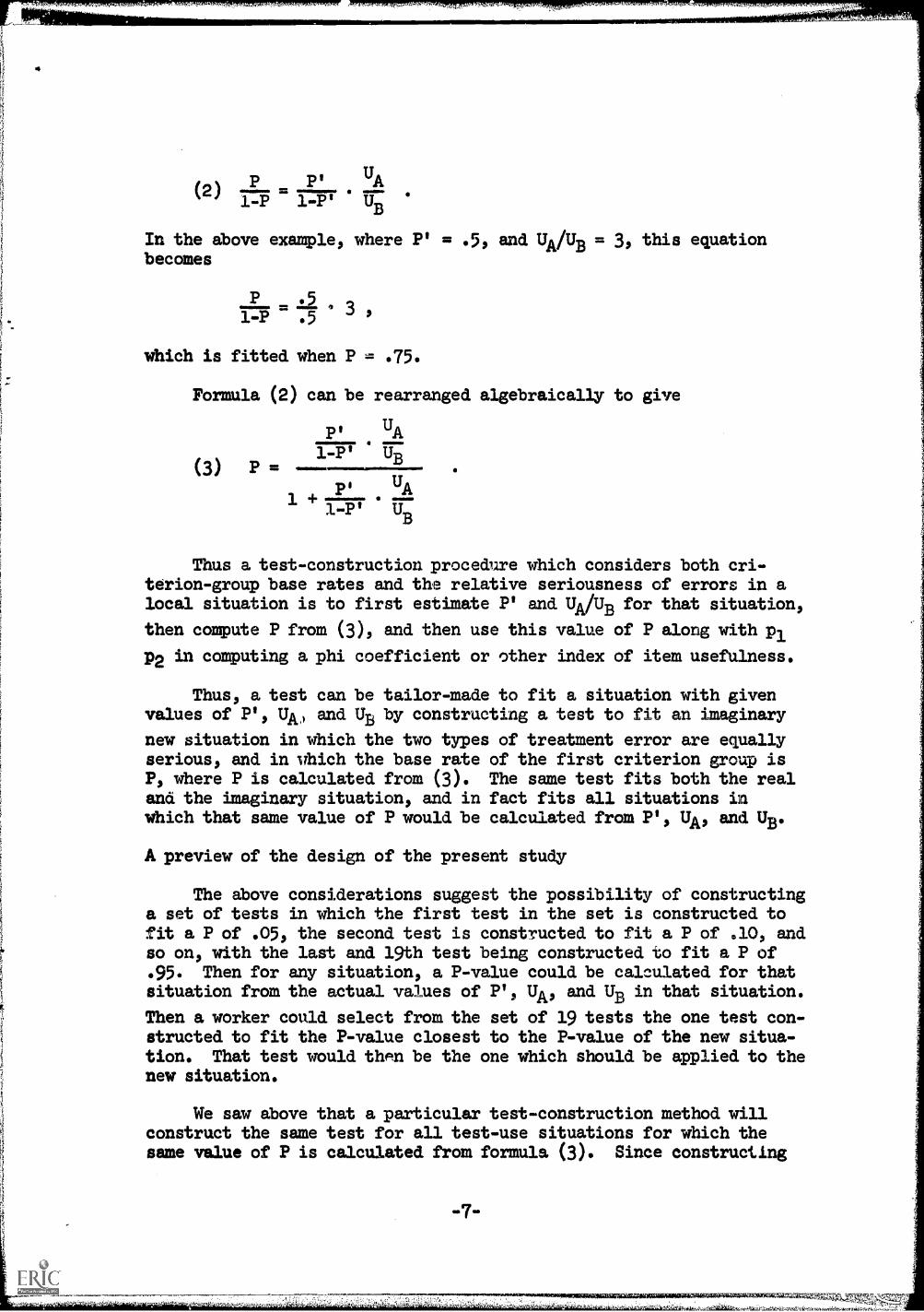
UA(2) P = P ----

1-P 1-PI UB

In the above example, where P' = .5, and UA /UB = 3, this equationbecomes

P -c

1-P3

.5 '

which is fitted when P = .75.

Formula (2) can be rearranged algebraically to give

(3) P

UP' UA1-P' U73

01111111M

Pi UA+ 171ST

Thus a test-construction procedure which considers both cri-terion-group base rates and the relative seriousness of errors in alocal situation is to first estimate P' and UA/UB for that situation,

then compute P from (3), and then use this value of P along with pi

p2 in computing a phi coefficient or other index of item usefulness.

Thus, a test can be tailor -made to fit a situation with givenvalues of P', UA, and UB by constructing a test to fit an imaginary

new situation in which the two types of treatment error are equallyserious, and in which the base rate of the first criterion group isP, where P is calculated from (3). The same test fits both the realand the imaginary situation, and in fact fits all situations inwhich that same value of P would be calculated from P', UA, and UB.

A preview of the design of the present study

The above considerations suggest the possibility of constructinga set of tests in which the first test in the set is constructed tofit a P of .05, the second test is constructed to fit a P of .10, andso on, with the last and 19th test being constructed to fit a P of.95. Then for any situation, a P-value could be calculated for thatsituation from the actual values of P', UA, and UB in that situation.

Then a worker could select from the set of 19 tests the one test con-structed to fit the P-value closest to the P-value of the new situa-tion. That test would then be the one which should be applied to thenew situation.

We saw above that a particular test-construction method willconstruct the same test for all test-use situations for which thesame value of P is calculated from formula (3). Since constructing

-7-

a test involves comparing the values of items, another way of statingour conclusion is that the relative values of items in a situationcan be computed merely from knowing P for the situation; the valuesof P', UA, and 1j/i3 need not be known separately. But what is true for

items should also be true for tests; it should be possible to com-pute the relative values of several tests in a situation from know-ing only the P-value of the situation. Thus if we have a set oftests, the same test should be the best test in the set for allsituations with the same value of P.

We are thus led to the following conclusion. Suppose a tablewere available in which the first column shows the relative valuesof each of several tests in a situation in which the base rate ofthe first criterion group is .05 and in which the two types of treat-ment error are equally serious. Suppose the second column of thetable shows the relative values of those same tests in a situationin which the base rate of the first criterion group is .10 and inwhich the two types of treatment error are equally serious. Suppose

that there are 19 columns of the table altogether, each showing therelative values of the tests in situations with different base ratesbut keeping the assumption that the two types of treatment error areequally serious. The base rate for the third column would be .15,for the fourth would be .20, and so on, with the base rate for the19th column being .95. Then if there were a real-life situation inwhich the two types of treatment error were not equally serious, itwould be possible to calculate P for that situation from formula (3),and then go to the column of the table with the base rate closest tothat P. The entries in that column would then show quite accuratelythe relative values of those several tests in that real-life situation.

Suppose further that the several tests whose values were listedin the table were the 19 tests referred to above, constructed to fit19 different values of P. Then the first entry in the first columnof the table would be the value, in a situation in which P = .05, ofa test constructed to fit a situation for which P equals that samevalue of .05. Going down the column would give the values in thatsame situation of tests constructed to fit increasingly differentP-values. Hence the first entry would be expected to be the highestentry in the first column. By the same reasoning, the highest entryin the second column would be expected to be the second entry, andin general the highest entry in each column would be expected to bethe entry falling on a diagonal line running from the upper left cor-ner of the table to the lower right corner. In any given column ofthe table, the farther away an entry is from this diagonal line, thesmaller the entry would be expected to be.

But how much smaller would these entries be than the entries nearthe diagonal? If they are much smaller, it would mean that it is veryimportant, when constructing a test for a specific situation, to usein the test-construction process the exact P-value which applies tothat situation. If the entries far from the diagonal are only very

slightly smaller than the entries near the diagonal, it would meanthat it is not very important to consider a situation's P-value whenconstructing a test to be used in that situation. It would furtherimply that a single test could be used in situations with diverseP-values, with results almost as good as could be achieved by con-structing many tests to fit the different situations.

The present project constructed 12 such 19 x 19 matrices. Eachmatrix was the result of applying a different one of four test-construction methods to a different one of three sets of data.

More preliminary work

Before we turn in more detail to the design of the project, wemust first consider the second of the two questions posed above.The first question, which we have now answered, is how we take intoconsideration, in the process of test construction, the base ratesand relative seriousness of the two types of treatment errors. Thesecond question, to which we now turn, is how we estimate the "value"of a test, or at least the relative values of two tests, in a situ-ation with specific values of P' and U.A. and UB.

This question was considered in two papers by Darlington andStauffer (3, h). The second of these two papers describes a methodfor finding the optimum cutting poini on a test (that is, the pointsuch that people with test scores above the point should receivetreatment A while people with test scores below the point shouldreceive treatment B) as a function of the mean test scores of thetwo groups of people, the standard deviations of the test scores ofthe two groups, and the relative seriousness of the two types oftreatment error. The formula assumes that the test scores of eachof the two groups of people are normally distributed..

Once this cutting point has been found, the only characteris-tics of the test which are relevant to its evaluation are the pro-portions of each of the two criterion groups with scores falling oneach side of the cutting point. Since the test has thus been dichoto-mized by the cutting point, it can be evaluated by using the sameformulas used to evaluate a dichotomous item. The procedures forevaluating such a dichotomous item were described in the first ofthe two papers by Darlington and Stauffer. That paper is basicallyan exposition of elementary decision theory as it is applied to theuse and evaluation of discrete tests. Fortunately, in the presentstudy we can avoid most of the complications in that paper, becausewe have seen above that we need to measure test values directly onlyin situations in which the two types of treatment error are equallyserious. In such cases the obvious measure of test value is simplythe number of correct classifications made by the test, expressed asa proportion of the total number of classifications made. In thepresent project, we subtracted from this number the base rate of thelarger criterion group (that is, the larger of the two numbers P and

-9-

1-P), since this is the proportion of the total population which

could be classified correctly if we simply classified everyone, in

the absence of any test information, in the larger of the two cri-

terion groups. Thus the actual measure of test value, which we will

call V, is the increase in the overall proportion of correct classi-

fications resulting from use of the test. For example, if a given

test classifies correctly .8 of the members of the first criterion

group, and .7 of the members of the second, and if P is .6, then the

overall proportion of correct classifications made by the test is

.8 .6 + .7 .4, or .76, so V, the value of the test, is

.76-.6, or .16. If cA is the proportion of the first criterion group

classified correctly by the test, and cB is the proportion of the

second criterion group correctly classified, and if M is defined as

the larger of the two numbers P and (1-P), then our definition of

V amounts to

V = cAP + cB(1-P)-M.

This formula provides the answer to the second of the two questions

raised above--how do we measure the value of a test?

A proof

In the foregoing discussion we have relied on the reader's

intuition to establish the point that the relative values of several

tests will be the same in all situations for which the same value

of P is calculated from formula (3). We will now establish this

point more formally. The present subsection can be skipped by readers

who are already convinced of the truth of the assertion.

The seriousness of decision errors can be measured in any con-

venient units. In mental hospital settings, it might be measured in

the number of months by which a patient's stay is lengthened as a

result of being assigned to an inappropriate treatment. In indus-

trial and commercial settings the unit of measurement is usually

dollars. Although a measure in dollar terms is often not appropriate

in educational settings, we will nevertheless use this in an example,

because of ilds ready understandability and simplicity.

Consider a situation in which P' = .6, UA = $3, and UB = $5.

Assume that the first criterion group (whose (Daze. rate is P') is the

group for which treatment 1 is appropriate, and that the second group

(whose base rate is 1-P') is the group for which treatment 2 is

appropriate. Then suppose treatment 1 were being given to everyone

and it was being considered whether treatment 2 would be better. From

the above numbers we see that for .6 of the total group, a switch to

treatment 2 would produce a loss of $3 per person, while for .4 of

the total group it would produce a gain of $5 per person. Thus the

-10-

Anol,a(C.1.1111.2aft,..1-1/VaL5-761.7,-41,CS,R5.1.17,t,tra^WMT14,,,,,,,711,

average gain resulting from the shift is

.4 $5 - .6 $3,

or $2.00 - $1.80, or $.20. Thus the average gain is positive, andtreatment 2 is better for the total group if no test is being used.

Suppose now a test is introduced which correctly classifies .8

of group 1 and .7 of group 2. Consider the strategy of giving treat-

ment 1 to everybody above the cutting point (that is, oil the side of

the cutting point toward which most members of the first group fall),

and treatment 2 to everybody below the cutting point. Switching to

this strategy and away from -Ghc strategy of giving treatment 2 to

everybody (which was the best strategy available without use of a

test) produces the following results:

(a) the proportion of the first criterion group treated cor-rectly rises from 0 to .8, at an average gain of $3 per

person correctly classified. Thus the mean gain for this

group is .8 $3, or $2.40.

(b) the proportion of the second criterion group treated cor-rectly falls from 1.0 to .7, at an average loss of $5 per

person incorrectly classified. Thus the mean loss for

this group is .3 $5, or $1.50.

Recalling that the base rates for the two groups are .6 and .4, the

mean gain in the two groups taken together resulting from using the

test is

.6 $2.40 - .4 $1.50

or $1.44 - $.6o, or $.84. Since introducing the test has resulted

in a mean gain of $.84 per person in the two groups together, $.84

is called the mean value per person of the test, which we denote by

V. V is the measure of test value used in this report.

Consider now the problem of stating the procedure just described

in terms of an algebraic formula. Let cA and cB be the proportions

of the two criterion groups correctly classified by the test. (In

the above example, cA was .8 and cB was .7.) Recalling that UA was

$3 and UB was $5, we see that $2.40 in the above example was cA UA,

and $1.50 was (1 - cB) UB. Recalling that .6 and .4 represented

P' and (1-P') respectively, the above procedure amounted to using the

formula

This formula simplifies algebraically to

(4) V = P'UAcA + (1-P')UBcB - (1-P')UB.

If we were to repeat the above line of reasoning in an example inwhich the treatment best for group A was the treatment which shouldbe used for everyone in the absence of a test, we would arrive atthe formula

(5) V = P'UAcA + (1-P')UBcB - PTA

instead of (4).

Formulas (4) and (5) give the value of a test in situations ofthe sort considered in this paper. Consider now the ratio betweenthe value of two tests j and k. Let cAj and cBj be the proportions

of the two criterion groups classified correctly by test j, and letcAk

and cBk be the proportions of the two criterion groups classified

correctly by test k. Starting with (4), the ratio of the values ofthe two tests is

V. pluAcm+ (1-P')UBcBj - (1-P')UB

(14"-YUB/ Vit P' A Akc + (1P-' U

Dividing both the numerator and denominator of the right side of (6)by (1-POUB gives

! 4tc . + c . .. 1

V Q.

U121p ut AJ BJ

(7) 17;

1-P'B Ak Bk

c c - 1

If we had started with (5) instead of with (4), we would have gotten

(1.4), UB

V cAj+`

UA cBj 1

( ) Vk UB

cAk P' ) cBk

Thus (7) gives the ratio of the value of two t-cnts when the treat-ment appropriate to the second group is the best treatment to giveeveryone in the absence of a test, and (8) gives that ratio whenthe treatment appropriate to the first group is the best treatmentto give everyone in the absence of a test.

No matter whether (7) or (8) is the appropriate formula for therelative value of two tests, inspection of the formula shows that

4

the relative value of two tests in a specific situation is affectedonly by the proportions of the two groups correctly classified by eachof the tests (these proportions are unaffected by P', UA, and UB), andby the value of

15,UA

1-P' UB

for the situation. But formula (2) shows that any two situationswhich have he same P value will also have the same value of

P' UA...--

1-P' UB

We thus reach the conclusion we sought to prove in the present sub-section: the relative values of several tests are the same acrossall situations which have the same value of P.

Method

In reading the following procedures, it should be rememberedthat the primary purpose of this project is to make a statement aboutthe general importance, for any type of prediction problem and anytest construction method, of tailor-making a test to fit a specificsituation. The descriptions of the specific data sets used are thusbriefer (in accordance with the request for brevity in the Instruc-tions) than they would be if we were interested in those data fortheir own sake. To a much smaller extent, this is also true of thedescriptions of the test-construction methods used.

Subjects and test-construction problems

Three different test-construction problems were used. The firstproblem involved using the MMPI to discriminate 96 hospitalizedschizophrenics from 250 nonschizophrenic mental hospital inpatients.The second involved discriminating 112 high-IQ children from 115retarded children, through the responses of each child's mother tothe 600-item Children's Personality Inventory. The third involvedusing the MMPI to discriminate 136 paranoid schizophrenic mentalhospital inpatients with low scores on the MMPI paranoid scale, from134 nonschizophrenic inpatients with low scores on the paranoidscale. In the first set of data, 29 schizophrenics and 83 nonschi-zophrenics were set aside as a cross-validation sample. In thesecond set, 40 high-IQ children and 40 low-IQ children were setaside -. In the third set, 48 patients from each of the two criteriongroups were set aside. The remainder of each set of data wasregarded as the test-construction sample in the analyses describedbelow.

, earahogtiinrit

-13-

Azi4 , .M,7 r 4 .

Test construction cess

For each of the above-described three sets of data, four setsof 19 tests each were constructed. Thus the total number of testsconstructed was 3 x 4 x 19, or 228. The four sets of tests differedfrom each other in that each set used a different test-constructionmethod. The 19 tests within a set differed from each other only inthe value of P assumed in the item-selection process. In the firsttest within each set: P was .05. In the second test within eachset, P was .10. For the third, fourth, and other tests within eachset, P was .15, .20, ..., .95.

As was just mentioned, four test-construction methods wereused. All four of these methods were procedures for selecting,from a pool of several hundred items, a smaller number of itemsfor inclusion in a test. In all cases, the selected items receivedunit weights; there was no attempt at differential weighting. Twoof the four methods of evaluating items used just P and pl and p2,

the proportions of the two criterion groups answering "Yes" to theitem. The other two methods used additional information which willbe described later in this subsection. Within the bounds of thestudy, the four methods were chosen to represent the major types oftest-construction methods in general use.

Method 1 was the method which was described in detail in theIntroduction, using the phi coefficient (0). The four numbers a,b, c, and d were computed for each item by the formulas

a =p1P

b = (1-p1)P

=p2(1-P)

d = (1-p2)(1-P).

For each item, 0 was then computed by formula (1). The 36 itemsfor which the absolute value of 0 was highest were selected for thetest. Of course, for the items in the 36 for which 0 was negative,the scoring direction of the item was reversed before the item wasincluded in the test. That is, if 0 for an item was positive thena "Yes" answer increased the subject's test score. If 0 for theitem was negative, then a "No" answer increased his score.

Method 2 was more complicated, It used a technique describedby Darlington and Bishop (2). The intent of the technique is tostart with a "first - stage" test, then to add to that first-stagetest those items in the item pool which are most able to improvethat test. The ability of an item to improve the first-stage testincreases with the item's validity, but decreases as the item's cor-

relation with the first-stage test increases. The specific indexused to measure an item's ability to improve the first-stage test was

.1011111WMPOR101.61.01.40,..

the partial correlation between the item and the criterion variable,partialling out the first-stage test. For each of the 19 tests con-structed by Method 2 for a particular one of the three sets of data,the test used as a first-stage test was the test constructed byMethod 1 for that same data set and that same value of P.

The partial correlation coefficient is computed from the threesimple correlation coefficients rci, rct, and rit, where c is the

criterion variable, t is the first-stage test, and i is the item

in question.

It will be recalled that tie purpose of the test-constructionphase of the project was to construct, from a single set of data,a series of tests in which each test was designed to fit a situa-

tion with a different value of P, where P is thought of as the base

rate of the first criterion group in an imaginary situation in

which the two types of treatment error are equally serious. Thus

in Method 2 we face the problem of estimating, from the single set

of data, the values which rci, rct, and rit would have in situa-

tions with different values of P. The item-criterion correlationrci is the only one of these three correlations which we have

essentially already discussed. Since c and i are both dichotomous,the correlation between them is the phi coefficient, and we des-

cribed in the Introduction the means for estimating the value which

a phi coefficient would assume in a population with a given value

of P. We must now consider rct and rit. Since t is a continuous

variable (the first-stage test), both rct and rit are point-biserial

correlations. We will consider first the problan of estimating,from a single set of data, the values which rct would assume in

populations with different values of P.

The basic problem is to express the point-biserial correlation

coefficient as a function only of P and of several quantities which

would not be expected to differ across populations with different

values of P. We faced a similar question earlier in connectionwith estimating the values which phi coefficients would assume in

situations with different values of P, and we solved it by expres-sing the entries in the phi coefficient (that is, a, b, c, and d)

as functions of P and pl and p2, the proportions of the two criterion

groups answering "Yes" to the item in question. These numbers pl

and p2 fit the above-mentioned specification--they would not be

expected to differ in populations with different values of P. The

problem is to find a similar set of numbers, and a set of formulas

for computing the point-biserial correlation coefficient from them.

Expressing rct in terms of the familiar formula for a point-

biserial correlation gives the formula

-15-

gi

r =13

1176.-0ct st

where TA and TB are the mean test scores of the two criterion groups

respectively, and where st is the overall standard deviation of thetest scores. P is, as throughout this paper, the assumed base rateof the first criterion group in the situation for which the test isto be constructed, and in which the two types of treatment error areimagined to be equally serious. The .quantities TA and TB are alreadyexpressed in acceptable form, since they would not be expected tovary across several populations which differed only in P. However,at is not in acceptable form; in general, the standard deviation ofthe test would be affected by P. This problem is handed as follows.

First express st in terms of the familiar standard deviationformula

ZT2 -2- Tst

where T's are individual test scores and T is the overall mean ofthe test scores. But T can be thought of as a weighted average ofTA and TB, wheee the weights are P and (1-P). That is,

= P YA + (1-IP) f136

TA and TB fit our stipulation for entries into rci' they should not

vary across populations with different values of P.

The term -2.--T2/N which appears in the formula for st can behandled in much the same way we just handled T. It is actually the

mean value of T2 in the population, so it can be expressed by

2E TN = P + (1-P) T

2

B 'T2

2 2where TfiLand TB are the mean values of T2 in the first and second

criterion groups respectively.

Thus we proceed as follows in estimating the value which !bet

would have in a situation with a given value of P. We enter thatvalue of P into the last two formulas, along with the values of TA,

B*P .10T2 and T2 observed in our sample data. The values of TA and

ZT2it thus computed are entered into the above formula for st.That value of st is then entered into the above formula for ret,along with the same values of "fm 110 and P used before.

A similar procedure was used to find rit, which like rci isa point-biserial correlation coefficient.

Once rev rot, and rit were found by the procedures describedabove, they were entered into the partial correlation formula

r - r rel ct -itr

ci.tN/ 1 - rr

ct -I-rit

0

This quantity was computed for each of the several hundred items inthe item pool, for each of the 19 values of P. For each value of P,the 9 items for which the absolute value of rci.t was highest wereadded to the 36-item first-stage test to form a 45-item second-stagetest. For reasons analogous to those described in connection withMethod 1, the items for which reit was negative were scored negatively.

Method 3 was quite different from Methods 1 and 2. We saw inthe Introduction the formulas which would be used if one were toevaluate a test or a dichotomous item in terms of the increase inthe proportion of correct classifications resulting from use of thetest or item. These same formulas provided the basis for item selec-tion in Method 3. That is, in each of the three sets of data andfor each of the 19 values of P, we computed the estimated increase inthe proportion of correct classifications resulting from using eachitem (alone, not in a test). This is a measure of item usefulnesswhich is similar to, but definitely different from, the phi coeffi-cient relating the item to the criterion variable. Since the formulasused were described in detail in the Introduction, we will not repeatthem here, even though there the discussion was in terms of testsand here the discussion is in terms of individual items. The formu-las are the same in the two cases. Once these numbers were computedfor a given set of data and a given value of P, the 36 items forwhich the numbers were highest were selected for a test. As in theother methotts, the entire procedure was repeated 19 times, for dif-ferent values of P, within each of the three sets of data.

Method 4 was the only one of the four test-construction methodswhich was developed for this project. It was by far the most compli-cated of the four test - construction methods. We found that it wasalso by far the most consuming of computer time; problems for whichMethods 1, 2, and 3 took about 5 minutes each, consumed about 2 hoursof the computer's time for Method 4. Later, on cross-validation, the

-17-

tests constructed by Method 4 were not noticeably better than those

constructed by other methods. Method 4 was thus basically a "flop."

For completeness, we will nevertheless include here a description

of the method.

Method 4 had much the same relation to Method 3 that Method 2

had to Method 1. That is, Methods 1 and 2 were both within a cor-

relational framework, and Method 2 used as first-stage tests the

tests constructed by Method 1. Methods 3 and 4 were both within the

framework of measuring item value by the increased proportion of cor-

rect classifications resulting from use of the item, and Method 4 used

as first-stage tests the tests constructed by Method 3. The essence

of Method 4 was a method for estimating which items, when added to a

test constructed by Method 3, would raise by the largest amount the

proportion of correct classifications resulting from use of the test,

assuming that the test scores are normally distributed within each

of the two criterion groups. This was done by adding each item in

the item pool separately to the 36-item first-stage test, then com-

puting the mean and standard deviation of test scores for each of

the two criterion groups. These means and standard deviations were

then entered into the above-mentioned formula developed by Darlington

and Stauffer (4) fc:- finding the optimum cutting point on the test.

Once the cutting point was found, normal curve tables were used to

compute, from the mear and standard deviation of test scores for each

criterion group, the proportion of each criterion group falling on

the correct side of the cutting point. These two proportions were

then weighted by P and (1-P) to give an estimate of the overall pro-

portion of correct classifications resulting from use of the original

36-item test with the one additional item added to it. This pro-

cedure was repeated hundreds of times, each time using as the one

additional item a different one of the several hundred items in the

item pool. The 9 items for which this statistic (the overall pro-

portion of correct classifications) was highest, were then added all

at once, as 9 items had been added all at once in Method 2, to the

original 36-item test to form a 45-item test. As in the previous

three methods, this procedure was repeated using 19 different values

of P in each of three sets of data.

Cutting points

We have mentioned earlier that the correct cutting point for

a test depends upon the P-value of the situation in which the test

is to be used. Construction of the 19 x 19 value matrices mentioned

above involves measuring the value of eacia of the above tests in

situations with different values of P. Hence for each test we calcu-

lated the optimum cutting point for each of the 19 values of P.

Besides P, the entries in this formula are the means and standard

deviations of the test scores for each of the two criterion groups.

These means and ,tandard deviations were computed in the test-

construction samples, and the 19 cutting points for each test were

then calculated.

Cross-validation and the value matrices

We have described above a process by which 4 sets of 19 testseach were constructed for each of three sets of test-constructionsample data. As mentioned earlier, corresponding to each of thesesets of data was a cross-validation sample of data, which had notbeen used in the test-construction process. Using exclusively thesecross-validation sample data, twelve 19 x 19 matrices of test valueswere constructed by the method outlined in the introduction. Con-structing each of these 12 matrices involved the following steps:

(a) Let cAjk and cBjk be the proportions of the two criterion

groups classified correctly, in the cross-validation sample, by the

.11th test with its kth cutting score, where subjects with test scoresabove the cutting point are classified as being in the first cri-terion group, and subjects with scores below the cutting point areclassified as being in the second criterion group. Then cAjk and

cut were computed for each value of j and each value of k from 1

to 19, forming a 19 x 19 matrix of values for each of the two sta-tistics. cAjk and cBjk are the estimated proportions of correct

classifications in the two criterion groups achieved by applying

the eh of the tests to a population with the kth of the 19 valuesof P, with the cutting score on the test chosen to maximize thenumber of correct classifications for that value of P.

(b) If the kth value of P is denoted by pat, then

(9) cAjkPk cBjk(1-Pk)

is the estimated overall proportion of correct classifications by

the eh test when used in a population with base rate Pk, The

larger of the two values Pk and (1 -Pk) is the largest overall pro-

portion of correct classifications possible without the use of atest; it is achieved by classifying all persons as members of thelarger criterion group. If we define Ei as the larger of the two

values El, and (1-Ex), then subtracting Mk from (9) gives the esti-

mated increase in the number of correct classificatioals (expressedas a proportion of the total population) achieved by the use oftest 1. If we denote this quantity by Vjk, and term it the value

of the jth test in a population with base rate Pk, then we have

(10) Vjk = cAjk Pk cBjk (1-Pk)Mk.

Vjk was computed for each of the 19 values of j and 19 values of k,

forming a 19 x 19 matrix of test values. Each column of this matrixshowed the values of 19 tests in a situation with a specific valueof P. The -ationale for this procedure was described in detail on pp.7-10; those pages should be reviewed by readers for whom the presentprocedure or its :rationale seems unclear.

-19-

,. t^p 'Z11,0

,,.fK1171,1.,,,,,,...,-A, ,F2vg,;;,,i, ,..t,p.,..yy,Frome7g9,77.7,,,1111.Wi.,,T4i,,,,,,7:1,1;g7r:

,..

.............,

7.7

Each of the twelve 19 x 19 matrices constructed by this procedurerelated to a particular one of the four test-construction methodsand a particular one of the three sets of data. Each of the 12matrices showed the relative values, as estimated from cross-valida-tion sample data, of 19 different tests in each of 19 differentsituations with different values of P. The 19 different tests in amatrix had all been constructed using the same one of the four test-construction methods, but the 19 tests had been constructed indepen-dently so that they were tailor-made to fit situations with differentvalues of P.

Results

As described in the Introduction, the major question of interestin the present project was whether tests constructed for a situationwith a given value of P were more valuable in that situation thanwere tests which had been constructed to fit situations with dif-

ferent values of P. Phrased in different terms, are the entriesfalling on the upper-left-to-lower-right diagonal of a given oneof the 19 x 19 matrices noticeably larger than entries in the samecolumns but far from the diagonal? The answer to this question is

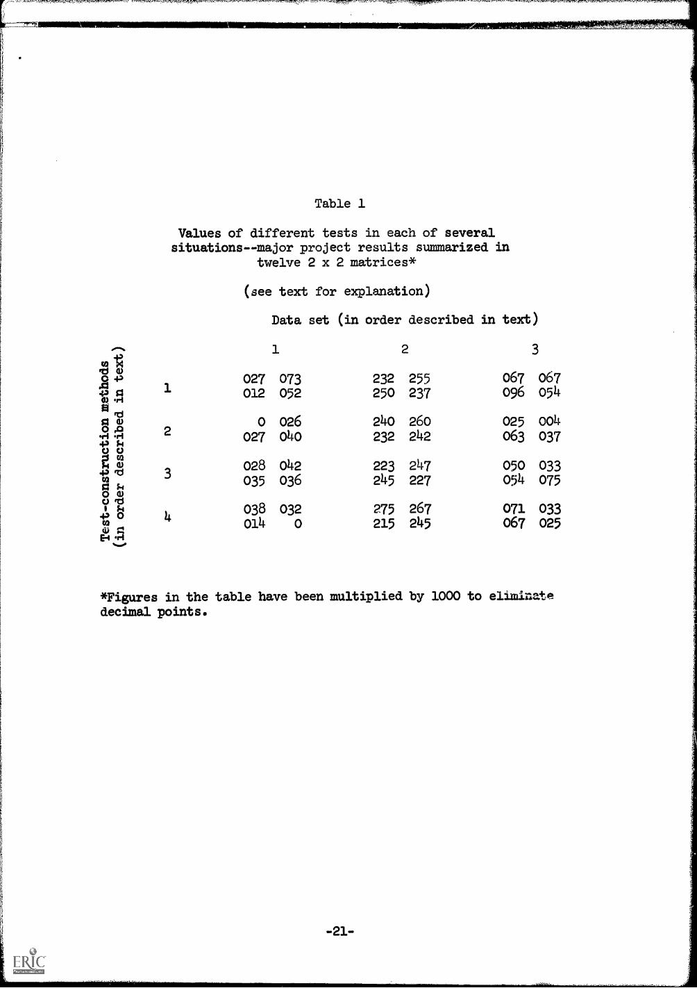
very simple: no. Although Table 1 shows only a small fraction ofthe total mass of data produced by the analyses described above, itis fully adequate to show the trend of the data. Table 1 contains

twelve 2 x 2 matrices. Each of these twelve 2 x 2 matrices containsfour elements from a different one of the twelve 19 x 19 matrices;the four elements show the value of each of two tests in situationswith two different values of P. In the first two of the three setsof data the P values used were .3 and .7. In the third set, testvalues were all very low for those P values, so P values of .4 and

.6 were used. In each of the twelve 2 x 2 matrices, the upper leftand lower right elements show the estimated vale of two tests inpopulations with the P values for which the test, 're designed. The

remaining two entries (lower left and upper right) show the estimatedvalue of each test in a population with the P value for which theother test was designed. Comparing the two numbers within a columnof any of the twelve matrices compares the estimated value, in apopulation with a given P, of a test constructed for that P, and atest constructed for a very different P. The former of the two num-bers would be predicted to be higher, the question being how muchhigher. Of the 24 such comparisons that can be made in Table 1, only8 (less than half) even show the difference to be in the predicted

direction. Nor are the differences in the predicted direction largerthan the others; if the 8 differences in the predicted directions areconsidered positive and the remaining 16 differences considered nega-tive, the mean of the 24 differences is negative. Further, inspec-tion of Table 1 shows that the 16 negative differences are not con-centrated in the results of any one of the four test-constructionmethods or in the results of any one of the three sets of data; theyare distributed across the four test-construction methods with the

-20-

1

2

3

14.

Table 1

Values of different tests in each of severalsituations - -major project results summarized in

twelve 2 x 2 matrices*

(see text for explanation)

Data set (in order described in text)

1 2 3

027 073 232 255 067 067012 052 250 237 096 054

0 026 240 260 025 004

027 040 232 242 063 037

028 042 223 247 050 033

035 036 245 227 054 075

038 032 275 267 071 033014 0 215 245 067 025

*Figures in the table have been multiplied by 1000 to eliminatedecimal points.

PiTA 7 77,77'

frequencies 5, 3, 5, 3, and across the three sets of data with the

frequencies 5, 6, 5.

Discussion and Conclusions

We conclude that for the types of test-construction problem

studied, tests tailor-made to fit the base rates and seriousness of

errors of a particular local situation are little (if any) better

in that situation than tests which were constructed for other situa-

tions. The results consistently supported this conclusion despite

the diversity in criterion variables, test-construction methods,

item pools, and samples of people studied.

The study, however, was confined to large item pools. Wilks

(5) has shown that the correlations among tests constructed by dif-

ferent Wghting methods can be expected to increase as the size of

the item pool from which the test items are drawn increases. It is

thus not certain whether the above conclusions apply when the item

pool is substantially smaller than the pools of 550 and 600 items

used in the present study.

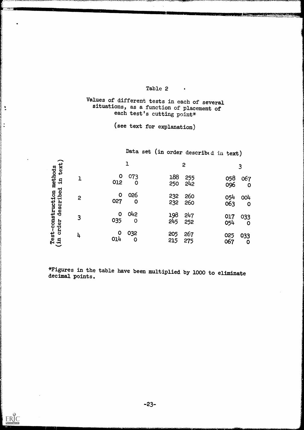
A Minor Parallel Study

A minor parallel study, using the data and tests already des-

cribed, was carried out on a question related to the major topic of

this project. This second question was whether the choice of cut-

ting point on a test greatly affects the value of the test for a

particular population. This part of the project is of limited

interest for two reasons: (a) it is quite simple to adjust the

cutting point on a test to fit any particular population, using

the Darlington-Stauffer technique mentioned above, so that the

question of how much is lost by failing to do so is unimportant;

(b) it seems obvious that the proper choice of cutting point would

have a great effect on test value. This expectation was fully

borne out by the data. The project consisted simply of repeating

the previous project, with the single change that in this second

phase the cutting point for a test was always left at the value

originally calculated for it using the P value for which the best

was constructed, rather than changing the cutting point to fit

new P values. The data in Table 2 are fully adequate to show the

trend of the data produced by this part of the project. As f.n

Table 1, the data are arranged in twelve 2 x 2 submatrices, each

submatrix corresponding to a different test-construction method

and data set. The upper right and lower left entries in each sub-

matrix are the same as in Table 1; they are thus values of tests

constructed for one value of P and evaluated in a population with

a very different P value. (The same P values were used as were

used in Table 1.) Each of these entries should again be compared to

the other element in the same column; this other entry is the value

-22-

/'Li 0O +'42

0

k

sr!+2

O kO a)Ord-P©O 0ri

%re

1

2

3

4

Table 2

Values of different tests in each of severalsituations, as a function of placement of

each test's cutting point*

(see text for explanation)

Data set (in order describtd is text)

1 2 3

o 073 188 255 058 067012 0 250 242 096 0

0 026 232 260 054 004027 0 232 260 063 0

0 042 198 247 017 033035 0 245 252 054 0

0 032 205 267 025 033014 0 215 275 067 0

*Figures in the table have been multiplied by 1000 to eliminatedecimal points.

of the same test in the same situation as the other entry in thatcolumn, but with the cutting point set for the value of P for whichthe test was originally constructed, rather than for the value ofP in the population in which test value is being measured.

Inspection of Table 2 shows that the choice of cutting pointmakes a large difference in test value. Of the 24 comparisons pos-sible between the two elements within a column of a submatrix inTable 2, all but two comparisons are in the predicted direction,usually by a substantial margin. The two exceptions (on the rightside of the last two submatrices in the center column) are both inthe data set for which test cross-validities were much higher thanare usually found in psychology, due to the nature of the criterionvariable (IQ, divided into superior and retarded groups). In such

data, most individuals are so far from the optimum cutting pointthat misplacing the cutting point should not be very serious, thusgiving rise to the two observed differences in the non-predicteddirection. In this respect, it is reasonable to believe that thesedata are atypical for psychology.

Summary

Users of standard psychological tests must regularly face thefact that the population of people for which a test was initiallydesigned differs somewhat from the local population to which thetest is to be applied. These users must regularly ask whetherthe time and expense involved in constructing a new test, tailor-made to the characteristics of the local population, would be re-paid by a noticeable improvement in predictive power, trhe presentpaper reports on an attempt to determine empirically, for severaltest-construction problems, the amount of improvement resultingwhen tests are tailor-made to fit one particular characteristic ofa local population--the base rates of the two criterion groups which

the test is designed to separate. The basic procedure used was toconstruct a series of tests which were alike in the item pool anditem-selection technique used, and in the two criterion groups whichthe tests were designed to separate, but which differed in the re-lative base rates of the two criterion groups assumed in the con-struction of the tests. Cross-validation sample data were thenused to estimate the value of each of the tests in populations witheach of the assumed base rates. The purpose was to estimate, foreach of these populations, the extent to which the test tailor-madefor that population exceeded in value tests tailor -made for popula-tions with different base rates. The results showed no noticeabledifference in the values of the various tests. These results wereconsistent across four different test-construction methods studied,and across three different sets of data which differed in the itempool and the criterion groups use d4) It is shown mathematicallythat the results imply that when decision-theory methods of test

-24-

I'S K177,13+1,_? 34,,IPINUrpft

construction and evaluation are used, no noticeable gain in testvalue results from explicitly considering the proper base ratesand the relative seriousness of the two types of misclassificationof subjects.

A minor parallel study showed that the choice of cutting pointon a test has a major effect on the test's value.

References

1. Cronbach, L. J., and Gleser, G. C. Psychological tests andpersounel decisions. Urbana: University of Illinois Press, 1957.

2. Darlington, Richard B., and Bishop, Carol H. "Increasing testvalidity by considering interitem correlations," Journ l ofAppladauchologx. 50, 1966, pp. 322-330.

3. Darlington, Richard B. and Stauffer, Glenn F. "Use and evalu-ation of discrete test information in decision making," Journalof Applied Psychology. 50, 1966, pp. 125-129.

4. Darlington, Richard B., and Stauffer, Glenn F. "A method forchoosing a cutting point on a test," journal of AppliedPsycholoa. 50, 1966, pp. 229-231.

5. Wilks, S. S. "Weighting systems for linear functions of cor-related variables when there is no dependent variable,"Psychometrika. 3, 1938, pp. 23-40.