R as an Environment for Reproducible Analysis of DNA ... · PDF fileR as an Environment for...
24
CONTRIBUTED RESEARCH ARTICLES 127 R as an Environment for Reproducible Analysis of DNA Amplification Experiments by Stefan Rödiger, Michal Burdukiewicz, Konstantin Blagodatskikh, Michael Jahn and Peter Schierack Abstract There is an ever-increasing number of applications, which use quantitative PCR (qPCR) or digital PCR (dPCR) to elicit fundamentals of biological processes. Moreover, quantitative isother- mal amplification (qIA) methods have become more prominent in life sciences and point-of-care- diagnostics. Additionally, the analysis of melting data is essential during many experiments. Several software packages have been developed for the analysis of such datasets. In most cases, the software is either distributed as closed source software or as monolithic block with little freedom to perform highly customized analysis procedures. We argue, among others, that R is an excellent foundation for reproducible and transparent data analysis in a highly customizable cross-platform environment. However, for novices it is often challenging to master R or learn capabilities of the vast number of packages available. In the paper, we describe exemplary workflows for the analysis of qPCR, qIA or dPCR experiments including the analysis of melting curve data. Our analysis relies entirely on R packages available from public repositories. Additionally, we provide information related to standardized and reproducible research. Introduction Quantitative polymerase chain reaction (qPCR) is the method of choice when a precise quantification of minute DNA traces is required. Applications include the detection and quantification of pathogens or gene expression analysis (Pabinger et al., 2014). Only few bioanalytical methods had such a significant impact on the progress of life sciences and medical sciences as the qPCR (Huggett et al., 2015b). Numerous commercial and experimental monitoring platforms have been developed in the past years. This includes standard plate cyclers, capillary cyclers, microfluidic platforms and related technologies (Rödiger et al., 2013b; Viturro et al., 2014; Rödiger et al., 2014; Khodakov and Ellis, 2014; Wu et al., 2014). In the past decades several isothermal amplification technologies emerged, such as helicase dependent amplification (HDA). Isothermal amplification methods were readily combined with real- time monitoring technologies (qIA) or digital PCR and are used in various fields like diagnostics and point-of-care-testing (Selck et al., 2013; Rödiger et al., 2014; Nixon et al., 2014). Digital PCR (dPCR) is a novel approach for detection and quantification of nucleic acids and can be seen as a next generation method (Huggett et al., 2015b). The dPCR technology breaks fundamentally with the previous concept of nucleic acid quantification. In contrast to traditional qPCR measures dPCR absolute nucleic acids amounts. This is possible after ‘clonal DNA amplification’ in thousands of small separated partitions (e.g., droplets, nano chambers; Huggett et al. 2013; Milbury et al. 2014; Morley 2014). Partitions with no nucleic acid remain negative and the others turn positive (e.g., Figure 1). Selected technologies (e.g., OpenArray®real-time PCR system) monitor amplification reactions in the chambers (‘partitions’) in real-time. After that, all quantification cycle (Cq) values are calculated from the amplification curves and converted into discrete events of positive and negative chambers. Finally, the absolute quantification of nucleic acids is done using Poisson statistics (Milbury et al., 2014; Morley, 2014). A representative workflow using the vendor software for the analysis of a droplet dPCR experiment has been described by Milbury et al. (2014). Recently, we have published the dpcR package (Burdukiewicz et al., 2015) at CRAN, which is the first open source R software package for the analysis of dPCR experiments (see the dpcR package manual for details). The complexity of hardware, wetware and software requires expertise to master a workflow. This comprises standards for experiment design, generation and analysis of data, multiple hypothesis testing, interpretation, reporting and storage of results (Huggett et al., 2014; Castro-Conde and de Uña-Álvarez, 2014). Scientific misconduct and fraud have shaken the scientific community on several occasions (Bustin, 2014). In particular, the scientific community works hard to uncover pitfalls of qPCR experiments. This led to the development of peer-reviewed quantification cycle (Cq) analysis algorithms (Ruijter et al., 2013), fully characterized qPCR chemistries (Ruijter et al., 2014) and guidelines for a proper conduct of qPCR experiments as implemented in the MIQE guidelines (minimum information for publication of quantitative real-time PCR experiments; Huggett et al. 2013; Bustin 2014). We share the philosophy of the MIQE guidelines to increase the experimental transparency for better experimental practice and reliable interpretation of results and encourage the The R Journal Vol. 7/1, June 2015 ISSN 2073-4859
Transcript of R as an Environment for Reproducible Analysis of DNA ... · PDF fileR as an Environment for...

CONTRIBUTED RESEARCH ARTICLES 127
R as an Environment for ReproducibleAnalysis of DNA AmplificationExperimentsby Stefan Rödiger, Michał Burdukiewicz, Konstantin Blagodatskikh, Michael Jahn and Peter Schierack
Abstract There is an ever-increasing number of applications, which use quantitative PCR (qPCR) ordigital PCR (dPCR) to elicit fundamentals of biological processes. Moreover, quantitative isother-mal amplification (qIA) methods have become more prominent in life sciences and point-of-care-diagnostics. Additionally, the analysis of melting data is essential during many experiments. Severalsoftware packages have been developed for the analysis of such datasets. In most cases, the softwareis either distributed as closed source software or as monolithic block with little freedom to performhighly customized analysis procedures. We argue, among others, that R is an excellent foundationfor reproducible and transparent data analysis in a highly customizable cross-platform environment.However, for novices it is often challenging to master R or learn capabilities of the vast numberof packages available. In the paper, we describe exemplary workflows for the analysis of qPCR,qIA or dPCR experiments including the analysis of melting curve data. Our analysis relies entirelyon R packages available from public repositories. Additionally, we provide information related tostandardized and reproducible research.
Introduction
Quantitative polymerase chain reaction (qPCR) is the method of choice when a precise quantification ofminute DNA traces is required. Applications include the detection and quantification of pathogens orgene expression analysis (Pabinger et al., 2014). Only few bioanalytical methods had such a significantimpact on the progress of life sciences and medical sciences as the qPCR (Huggett et al., 2015b).Numerous commercial and experimental monitoring platforms have been developed in the past years.This includes standard plate cyclers, capillary cyclers, microfluidic platforms and related technologies(Rödiger et al., 2013b; Viturro et al., 2014; Rödiger et al., 2014; Khodakov and Ellis, 2014; Wu et al.,2014).
In the past decades several isothermal amplification technologies emerged, such as helicasedependent amplification (HDA). Isothermal amplification methods were readily combined with real-time monitoring technologies (qIA) or digital PCR and are used in various fields like diagnostics andpoint-of-care-testing (Selck et al., 2013; Rödiger et al., 2014; Nixon et al., 2014).
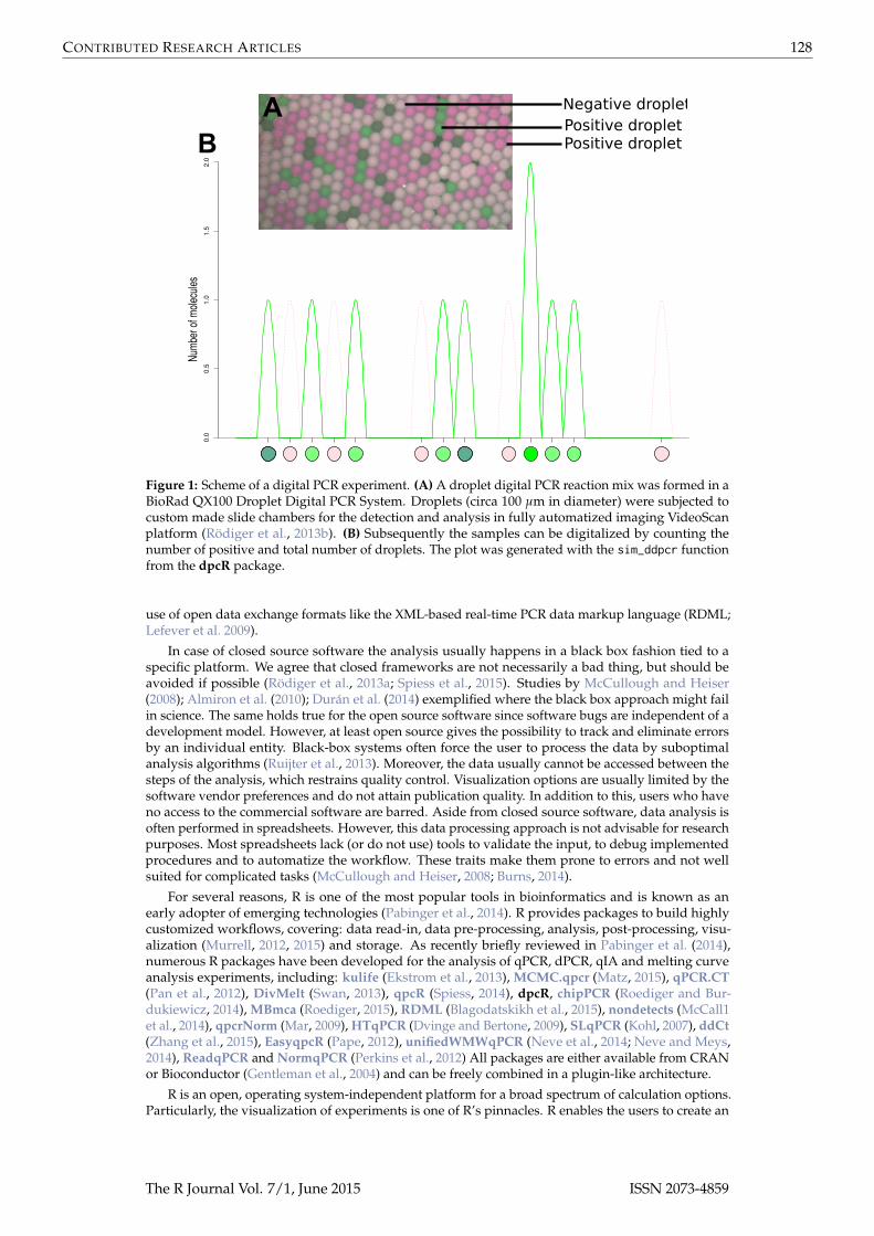
Digital PCR (dPCR) is a novel approach for detection and quantification of nucleic acids and can beseen as a next generation method (Huggett et al., 2015b). The dPCR technology breaks fundamentallywith the previous concept of nucleic acid quantification. In contrast to traditional qPCR measuresdPCR absolute nucleic acids amounts. This is possible after ‘clonal DNA amplification’ in thousandsof small separated partitions (e.g., droplets, nano chambers; Huggett et al. 2013; Milbury et al. 2014;Morley 2014). Partitions with no nucleic acid remain negative and the others turn positive (e.g.,Figure 1). Selected technologies (e.g., OpenArray®real-time PCR system) monitor amplificationreactions in the chambers (‘partitions’) in real-time. After that, all quantification cycle (Cq) values arecalculated from the amplification curves and converted into discrete events of positive and negativechambers. Finally, the absolute quantification of nucleic acids is done using Poisson statistics (Milburyet al., 2014; Morley, 2014). A representative workflow using the vendor software for the analysis of adroplet dPCR experiment has been described by Milbury et al. (2014). Recently, we have published thedpcR package (Burdukiewicz et al., 2015) at CRAN, which is the first open source R software packagefor the analysis of dPCR experiments (see the dpcR package manual for details).
The complexity of hardware, wetware and software requires expertise to master a workflow. Thiscomprises standards for experiment design, generation and analysis of data, multiple hypothesistesting, interpretation, reporting and storage of results (Huggett et al., 2014; Castro-Conde andde Uña-Álvarez, 2014). Scientific misconduct and fraud have shaken the scientific community onseveral occasions (Bustin, 2014). In particular, the scientific community works hard to uncoverpitfalls of qPCR experiments. This led to the development of peer-reviewed quantification cycle (Cq)analysis algorithms (Ruijter et al., 2013), fully characterized qPCR chemistries (Ruijter et al., 2014)and guidelines for a proper conduct of qPCR experiments as implemented in the MIQE guidelines(minimum information for publication of quantitative real-time PCR experiments; Huggett et al.2013; Bustin 2014). We share the philosophy of the MIQE guidelines to increase the experimentaltransparency for better experimental practice and reliable interpretation of results and encourage the
The R Journal Vol. 7/1, June 2015 ISSN 2073-4859
CONTRIBUTED RESEARCH ARTICLES 128
AB
Negative dropletPositive dropletPositive droplet
Figure 1: Scheme of a digital PCR experiment. (A) A droplet digital PCR reaction mix was formed in aBioRad QX100 Droplet Digital PCR System. Droplets (circa 100 µm in diameter) were subjected tocustom made slide chambers for the detection and analysis in fully automatized imaging VideoScanplatform (Rödiger et al., 2013b). (B) Subsequently the samples can be digitalized by counting thenumber of positive and total number of droplets. The plot was generated with the sim_ddpcr functionfrom the dpcR package.
use of open data exchange formats like the XML-based real-time PCR data markup language (RDML;Lefever et al. 2009).
In case of closed source software the analysis usually happens in a black box fashion tied to aspecific platform. We agree that closed frameworks are not necessarily a bad thing, but should beavoided if possible (Rödiger et al., 2013a; Spiess et al., 2015). Studies by McCullough and Heiser(2008); Almiron et al. (2010); Durán et al. (2014) exemplified where the black box approach might failin science. The same holds true for the open source software since software bugs are independent of adevelopment model. However, at least open source gives the possibility to track and eliminate errorsby an individual entity. Black-box systems often force the user to process the data by suboptimalanalysis algorithms (Ruijter et al., 2013). Moreover, the data usually cannot be accessed between thesteps of the analysis, which restrains quality control. Visualization options are usually limited by thesoftware vendor preferences and do not attain publication quality. In addition to this, users who haveno access to the commercial software are barred. Aside from closed source software, data analysis isoften performed in spreadsheets. However, this data processing approach is not advisable for researchpurposes. Most spreadsheets lack (or do not use) tools to validate the input, to debug implementedprocedures and to automatize the workflow. These traits make them prone to errors and not wellsuited for complicated tasks (McCullough and Heiser, 2008; Burns, 2014).
For several reasons, R is one of the most popular tools in bioinformatics and is known as anearly adopter of emerging technologies (Pabinger et al., 2014). R provides packages to build highlycustomized workflows, covering: data read-in, data pre-processing, analysis, post-processing, visu-alization (Murrell, 2012, 2015) and storage. As recently briefly reviewed in Pabinger et al. (2014),numerous R packages have been developed for the analysis of qPCR, dPCR, qIA and melting curveanalysis experiments, including: kulife (Ekstrom et al., 2013), MCMC.qpcr (Matz, 2015), qPCR.CT(Pan et al., 2012), DivMelt (Swan, 2013), qpcR (Spiess, 2014), dpcR, chipPCR (Roediger and Bur-dukiewicz, 2014), MBmca (Roediger, 2015), RDML (Blagodatskikh et al., 2015), nondetects (McCall1et al., 2014), qpcrNorm (Mar, 2009), HTqPCR (Dvinge and Bertone, 2009), SLqPCR (Kohl, 2007), ddCt(Zhang et al., 2015), EasyqpcR (Pape, 2012), unifiedWMWqPCR (Neve et al., 2014; Neve and Meys,2014), ReadqPCR and NormqPCR (Perkins et al., 2012) All packages are either available from CRANor Bioconductor (Gentleman et al., 2004) and can be freely combined in a plugin-like architecture.
R is an open, operating system-independent platform for a broad spectrum of calculation options.Particularly, the visualization of experiments is one of R’s pinnacles. R enables the users to create an
The R Journal Vol. 7/1, June 2015 ISSN 2073-4859

CONTRIBUTED RESEARCH ARTICLES 129
Figure 2: An exemplary workflow for quantitative PCR, digital PCR, quantitative isothermal am-plification and melting curve analysis experiments in R. The R software environment provides corefunctionality for statistical computing and graphics. In our scenario we used the RDML packageto read-in data in standardized format. However, any format supported by R can be used. Further,processing of amplification curve data was performed with the chipPCR package and melting curvedata were analysed with the MBmca package. The dpcR package can be embedded in the analysis ofdigital PCR experiments. Cq, quantification cycle; TM, melting temperature.
efficient manipulation, restructuring and reshaping of data to make them readily-available for furtherprocessing. This is of the particular importance to the human–machine interface (Oh, 2014). Intrinsicproperties of R such as naming conventions (Bååth, 2012) and class systems (e.g., S3, S4, referenceclasses and R6) vary considerable, depending on the package developer preferences. However, due tothe open source approach, there is the common ground to track numerical errors. R offers variousmethods for a standardized data import/export and exchange. Workflows can embed structuredmodels (Zeller et al., 2009), open data exchange formats (e.g., RDML), binary formats (Michna andWoods, 2013) or tools provided by the R workspace (R Core Team, 2015). The NetCDF binary format,available from the RNetCDF package (Michna, 2015), has advantages over some other binary formats(e.g., the RData format), since arbitrary array data sections of massive datasets can be processedefficiently (Michna and Woods, 2013). This might be useful for large data sets as present in high-throughput PCR experiments or dPCR experiments with large partition numbers. The R environmentoffers several datasets, which can be used for testing of algorithms. Therefore, we, among others,argue that R is suitable for reproducible research (Gentleman et al., 2004; Murrell, 2012; Gandrud, 2013;Hofmann et al., 2013; Ooms, 2013; Kuhn, 2015; Leeper, 2014; Liu and Pounds, 2014).
The aim of this paper is to show case studies for qPCR, dPCR, qIA and melting curve analysisexperiments. Our workflow effectively follows the principle illustrated in Figure 2. We intend toaggregate functionalities dispersed between various packages and offer a fast insight in the analysis ofnucleic acid experiments with R. In particular, we describe how to:
• read-in data from a standardized file format,
• pre-process the amplification curve data,
• calculate specific parameters from the amplification curve data,
• calculate the melting temperature,
• and report the data.
Setting-up a working environment
We recommend performing the scripting in a dedicated integrated development environment (IDE)and graphical user interface (GUI) such as RKWard (Rödiger et al., 2012), RStudio (RStudio, 2014;Gandrud, 2013) or other technologies (Valero-Mora and Ledesma, 2012). Benefits of IDEs withGUI include syntax-highlighting, auto completion and function references for rapid prototyping ofworkflows. Typically, the analysis will start with data from a commercial platform. Most platformshave an option to export a CSV file or spreadsheets application file (e.g., *.xls, *.odt). Details for thedata import have been described elsewhere (R Core Team, 2015; Rödiger et al., 2012). To keep the
The R Journal Vol. 7/1, June 2015 ISSN 2073-4859

CONTRIBUTED RESEARCH ARTICLES 130
case study sections compact we have chosen to load datasets from the qpcR package (Ritz and Spiess,2008) (v. 1.4.0) and the RDML package (v. 0.8-3) to our workspace. The chipPCR package (Rödigeret al., in press) (v. 0.0.8-10) was used for data pre-processing, quality control and the calculation of thequantification cycle (Cq).
The Cq is a quantitative measure, which represents the number of cycles needed to reach a userdefined threshold signal level, in the exponential phase of a qPCR/qIA reaction. Several Cq methodshave been described (Ruijter et al., 2013). In this study we have chosen the second derivative maximummethod (CqSDM) and the ‘Cycle threshold’ (CqCt) method.
During a perfect qPCR reaction, the target DNA doubles (2n; n = cycle number) at each cycle. Herethe amplification efficiency (AE) is 100 %. However, in reality, numerous factors cause an inhibition ofthe amplification (AE < 100 %). The AE can be determined by the relation of the Cq value dependingon the sample input quantity as described in (Rödiger et al., in press; Svec et al., 2015).
In Rödiger et al. (2013a) we described the application of R for the analysis of melting curveexperiments from microbead-based assays. We used functions from the MBmca package (0.0.3-4) foran analysis of the target specific melting temperature (TM) in experiments of the present study, sincethe mathematical foundation is the same.
We completed our examples with case studies for the analysis of dPCR experiments. In particular,we used the dpcR package (v. 0.1.4.0) to estimate the number of molecules in a sample.
Results
In the following sections we will show how R can be used (I) as a unified open software for dataanalysis and presentation in research, (II) as software frame-work for novel technical developments,(III) as platform for teaching of new technologies and (IV) as reference for statistical methods.
Case study one – qPCR and amplification efficiency calculation
The goal of our first case study was to calculate the Cq values and the AE from a qPCR experiment. Weused the guescini1 dataset from the qpcR package, where the gene NADH dehydrogenase 1 (MT-ND1)was amplified in a LightCyclerr 480 (Roche) thermocycler. Details of the experiment are described inGuescini et al. (2008). We started with loading the required packages and datasets. A good practice forreproducible research is to track the package versions and environment used during the analysis. Thefunction sessionInfo from the utils package provides this functionality. Assuming that the analysisstarts with a clean R session it is possible to assign the required packages to an object, as shown below.Reproducibility of research can be further improved by the archivist package (Biecek and Kosinski,2015), which stores and recovers crucial data and preserves metadata of saved objects (not shown). Allsettings of an R session can be easily saved and/or restored using the settings package (van der Loo,2015).
# Load the required packages for the data import and analysis.# Load the chipPCR package for the pre-processing and curve data quality# analysis and load the qpcR package as data resource.require(chipPCR)require(qpcR)
# Collect information about the R session used for the analysis of the# experiment.current.session <- sessionInfo()
# Next, we load the 'guescini1' dataset from the qpcR package to the# workspace and assign it to the object 'gue'.gue <- guescini1
# Define the dilution of the sample DNA quantity for the calibration curve# and assign it to the object 'dil'.dil <- 10^(2: -4)
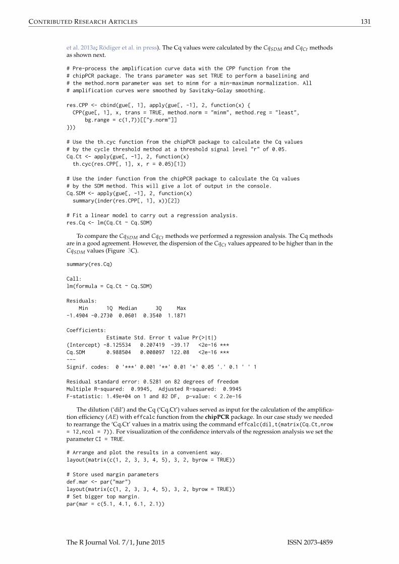
We previewed the amplification curve raw data using the matplot function (see code below). Theamplification curve data showed a strong signal level variation in the plateau region (Figure 3A).Therefore, all data were subjected to a minimum-maximum normalization using the CPP function fromthe chipPCR package. In addition, all data were baselined and smoothed (Figure 3B; see Rödiger
The R Journal Vol. 7/1, June 2015 ISSN 2073-4859
CONTRIBUTED RESEARCH ARTICLES 131
et al. 2013a; Rödiger et al. in press). The Cq values were calculated by the CqSDM and CqCt methodsas shown next.
# Pre-process the amplification curve data with the CPP function from the# chipPCR package. The trans parameter was set TRUE to perform a baselining and# the method.norm parameter was set to minm for a min-maximum normalization. All# amplification curves were smoothed by Savitzky-Golay smoothing.
res.CPP <- cbind(gue[, 1], apply(gue[, -1], 2, function(x) {CPP(gue[, 1], x, trans = TRUE, method.norm = "minm", method.reg = "least",
bg.range = c(1,7))[["y.norm"]]}))
# Use the th.cyc function from the chipPCR package to calculate the Cq values# by the cycle threshold method at a threshold signal level "r" of 0.05.Cq.Ct <- apply(gue[, -1], 2, function(x)th.cyc(res.CPP[, 1], x, r = 0.05)[1])
# Use the inder function from the chipPCR package to calculate the Cq values# by the SDM method. This will give a lot of output in the console.Cq.SDM <- apply(gue[, -1], 2, function(x)summary(inder(res.CPP[, 1], x))[2])
# Fit a linear model to carry out a regression analysis.res.Cq <- lm(Cq.Ct ~ Cq.SDM)
To compare the CqSDM and CqCt methods we performed a regression analysis. The Cq methodsare in a good agreement. However, the dispersion of the CqCt values appeared to be higher than in theCqSDM values (Figure 3C).
summary(res.Cq)
Call:lm(formula = Cq.Ct ~ Cq.SDM)
Residuals:Min 1Q Median 3Q Max
-1.4904 -0.2730 0.0601 0.3540 1.1871
Coefficients:Estimate Std. Error t value Pr(>|t|)
(Intercept) -8.125534 0.207419 -39.17 <2e-16 ***Cq.SDM 0.988504 0.008097 122.08 <2e-16 ***---Signif. codes: 0 '***' 0.001 '**' 0.01 '*' 0.05 '.' 0.1 ' ' 1
Residual standard error: 0.5281 on 82 degrees of freedomMultiple R-squared: 0.9945, Adjusted R-squared: 0.9945F-statistic: 1.49e+04 on 1 and 82 DF, p-value: < 2.2e-16
The dilution (‘dil’) and the Cq (‘Cq.Ct’) values served as input for the calculation of the amplifica-tion efficiency (AE) with effcalc function from the chipPCR package. In our case study we neededto rearrange the ‘Cq.Ct’ values in a matrix using the command effcalc(dil,t(matrix(Cq.Ct,nrow= 12,ncol = 7)). For visualization of the confidence intervals of the regression analysis we set theparameter CI = TRUE.
# Arrange and plot the results in a convenient way.layout(matrix(c(1, 2, 3, 3, 4, 5), 3, 2, byrow = TRUE))
# Store used margin parametersdef.mar <- par("mar")layout(matrix(c(1, 2, 3, 3, 4, 5), 3, 2, byrow = TRUE))# Set bigger top margin.par(mar = c(5.1, 4.1, 6.1, 2.1))
The R Journal Vol. 7/1, June 2015 ISSN 2073-4859
CONTRIBUTED RESEARCH ARTICLES 132
0 10 20 30 40 50
010
2030
4050
60
Raw data
Cycle
RF
U
A
0 10 20 30 40 50
0.0
0.2
0.4
0.6
0.8
1.0
Pre−processed data
Cycle
RF
U
B
●●●●●●●●●●●●
●●●●● ●● ●●● ●●
●●●●●●
●●●●●●
●●● ●● ●●● ●●● ●
●●●●●● ●●●●●●
● ●●
● ●●
●●● ●●●
●●●
●
● ●
●●●●●●
15 20 25 30 35
510
1520
25
Comparison of Cq methods
Cq Ct method
Cq
SD
M m
etho
d
C
●
●
●
●
●
●
●
−4 −3 −2 −1 0 1 2
510
1520
25
Efficiency Plot
log10(Concentration)
Cq
Ct m
etho
d
Efficiency = 96.2 %R^2 = 0.999r = −0.999; p < 0.001
D
●
●
●
●
●
●
●
−4 −3 −2 −1 0 1 2
1520
2530
35
Efficiency Plot
log10(Concentration)
Cq
SD
M m
etho
d
Efficiency = 95.6 %R^2 = 1r = −1; p < 0.001
E
Figure 3: Analysis of the amplification curve data of the guescini1 dataset. (A) Raw data from thecalibration curve samples were visually inspected. The qPCR curves display a broad variation inplateau fluorescence (38–62 RFU). (B) The CPP function from the chipPCR package was used to baselinethe data, to smooth the data with Savitzky-Golay smoothing filter and to normalize the data between0 and 1. The red horizontal line (—) indicates the fluorescence level (0.05) used for the calculationof the Cq value by the ‘cycle threshold’ method. (C) The Cq values were calculated by the CqSDMmethod (‘SDM method’) (inder, chipPCR) and the CqCt method (‘Ct method’) (th.cyc, chipPCR).The threshold value was set to r = 0.05. The CqSDM and CqCt values were plotted and analysedby a linear regression (R2 = 0.9945; P < 2.2−16) and Pearson’s r (r = 0.9972605; P < 2.2−16). Theamplification efficiency based on (D) CqCt values and (E) CqSDM values were automatically analysedwith the effcalc (chipPCR) function. Cq, Quantification cycle; SDM, Second derivative maximum,R^2, Coefficient of determination; r, Pearson product-moment correlation coefficient, RFU, relativefluorescence units.
The R Journal Vol. 7/1, June 2015 ISSN 2073-4859
CONTRIBUTED RESEARCH ARTICLES 133
# Plot the raw amplification curve data.matplot(gue[, -1], type = "l", lty = 1, col = 1, xlab = "Cycle",
ylab = "RFU", main = "Raw data")mtext("A", side = 3, adj = 0, cex = 2)
# Plot the pre-processed amplification curve data.matplot(res.CPP[, -1], type = "l", lty = 1, col = 1, xlab = "Cycle",
ylab = "RFU (normalized)", main = "Pre-processed data")mtext("B", side = 3, adj = 0, cex = 2)abline(h = 0.05, col = "red", lwd = 2)
# Plot Cq.SDM against Cq.Ct and add the trendline from the linear regression# analysis.
plot(Cq.SDM, Cq.Ct, xlab = "Cq Ct method", ylab = "Cq SDM method",main = "Comparison of Cq methods")
abline(res.Cq)mtext("C", side = 3, adj = 0, cex = 2)
# Use the effcalc function from the chipPCR package to calculate the# amplification efficiency.plot(effcalc(dil, t(matrix(Cq.Ct, nrow = 12, ncol = 7))), ylab = "Cq Ct method",
CI = TRUE)mtext("D", side = 3, adj = 0, cex = 2)
plot(effcalc(dil, t(matrix(Cq.SDM, nrow = 12, ncol = 7))), ylab = "Cq SDM method",CI = TRUE)
mtext("E", side = 3, adj = 0, cex = 2)
# Resore margin default values.par(mar = c(5.1, 4.1, 4.1, 2.1))
Finally, Cq values were plotted using the layout function (Figures 3D and E). The Cq valuesand amplification vary slightly between both methods. This is an expected observation and is inaccordance to the findings by Ruijter et al. (2013). As shown in this case study, it is easy to set-up astreamlined workflow for data read-in, pre-processing and analysis with a few functions.
Case study two – qPCR and melting curve analysis
A common task during the analysis of qPCR experiments is to distinguish between positive andnegative samples (see Figure 5). If the melting temperature of a sample is known it is possible toautomatize the decision by a melting curve analysis (MCA). As shown in Rödiger et al. (2013a) this canbe done by interrogating the TM. Therefore, we used a logical statement, which tests if TM is within atight temperature range. We used the signal height as second parameter. In line with ‘Case study one –qPCR and amplification efficiency calculation we used the function sessionInfo to track all packagesused during the analysis. Reproducible research is greatly enhanced if open data exchange formats areused. Therefore, we used the RDML package for data read-in. The amplification and melting curvedata were measured with a CFX96 system (Bio-Rad) and then exported as RDML v 1.1 format file as‘BioRad_qPCR_melt.rdml’. Within this qPCR experiment we amplified the Mycobacterium tuberculosiskatG gene and tried to detect a mutation at codon 315. The experiment was separated in two parts:
1. Detection of overall M. tuberculosis DNA (wild-type and mutant) and
2. specific detection of wild-type M. tuberculosis by melting of TaqMan probe (quencher – BHQ2,fluorescent reporter – Cy5) with amplified DNA (see Luo et al. 2011 for probe/primer sequencesand further details).
The qPCR was conducted using EvaGreenr Master Mix (Syntol) according to the manufacturer’sinstructions, with 500 nM of primers and probe in a 25 µL final reaction volume. Thermocycling wasconducted using a CFX96 (BioRad) initiated by 3 min incubation at 95 °C, followed by 41 cycles (15 s at95 °C; 40 s at 65 °C) with a single read-out taken at the end of each cycle. Probe melting was conductedbetween 35 °C and 95 °C by 1 °C at 1 s steps.
RDML file structures can be complex. Though RDML files are XML structured files and thusintended to be readable by humans, it is hard to grasp the complex hierarchical file structure withoutsome basic understanding. A simple and fast method to compactly display the structure of an object
The R Journal Vol. 7/1, June 2015 ISSN 2073-4859
CONTRIBUTED RESEARCH ARTICLES 134
in R is to use the str or summary function (not shown). However, such R tools are not informative inthis context. Therefore we implemented a dendrogram-like view (Figure 4). According to this, the filecontains different datasets, each with 3 samples, (‘pos’, ‘ntc’, ‘unknown’). Only a subset of the datawas used in our case study and combined to the object qPCR.
# Import the qPCR and melting curve data via the RDML package.# Load the chipPCR package for the pre-processing and curve data quality# analysis and the MBmca package for the melting curve analysis.require(RDML)require(chipPCR)require(MBmca)require(dplyr)
# Collect information about the R session used for the analysis of the qPCR# experiment.current.session <- sessionInfo()
# Load the BioRad_qPCR_melt.rdml file from the RDML package and assign the data# to the object 'BioRad'.filename <- file.path(path.package("RDML"), "extdata", "BioRad_qPCR_melt.rdml")BioRad <- RDML$new(filename)
# The structure of the file can be overviewed by the AsDendrogram() function.# We can see that our experiment contains two detection channels (Figure 4).# ('EvaGreen' and 'Cy5' at 'Run ID'). 'EvaGreen' channel has one# probe (target) - 'EvaGreen'. 'Cy5' has: 'Cy5', 'Cy5-2' and 'Cy5-2_rr'.# each target has three sample types (positive, unknown, negative).# And each sample type has qPCR ('adp') and melting ('mdp') data.# The last column shows the number of samples in an experiment.
BioRad$AsDendrogram()
# Fetch cycle dependent fluorescence for the EvaGreen channel and row 'D'# (contains the target 'Cy5-2' in the channel 'Cy5') of the# katG gene and aggregate the data in the object 'qPCR'.
qPCR <- BioRad$AsTable() %>%filter(target == "EvaGreen",
grepl("^D", position)) %>% BioRad$GetFData(.)
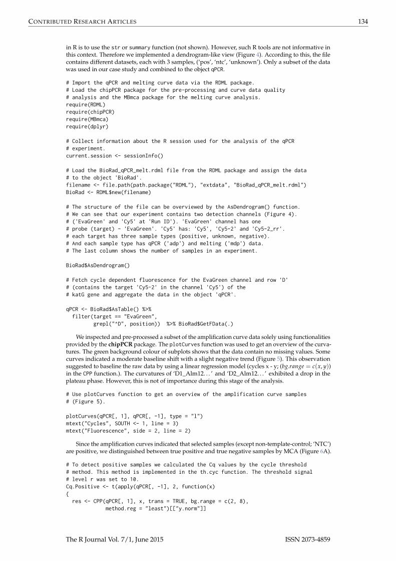
We inspected and pre-processed a subset of the amplification curve data solely using functionalitiesprovided by the chipPCR package. The plotCurves function was used to get an overview of the curva-tures. The green background colour of subplots shows that the data contain no missing values. Somecurves indicated a moderate baseline shift with a slight negative trend (Figure 5). This observationsuggested to baseline the raw data by using a linear regression model (cycles x - y; (bg.range = c(x, y))in the CPP function.). The curvatures of ‘D1_Alm12. . . ’ and ‘D2_Alm12. . . ’ exhibited a drop in theplateau phase. However, this is not of importance during this stage of the analysis.
# Use plotCurves function to get an overview of the amplification curve samples# (Figure 5).
plotCurves(qPCR[, 1], qPCR[, -1], type = "l")mtext("Cycles", SOUTH <- 1, line = 3)mtext("Fluorescence", side = 2, line = 2)
Since the amplification curves indicated that selected samples (except non-template-control; ‘NTC’)are positive, we distinguished between true positive and true negative samples by MCA (Figure 6A).
# To detect positive samples we calculated the Cq values by the cycle threshold# method. This method is implemented in the th.cyc function. The threshold signal# level r was set to 10.Cq.Positive <- t(apply(qPCR[, -1], 2, function(x){res <- CPP(qPCR[, 1], x, trans = TRUE, bg.range = c(2, 8),
method.reg = "least")[["y.norm"]]
The R Journal Vol. 7/1, June 2015 ISSN 2073-4859

CONTRIBUTED RESEARCH ARTICLES 135
All Wells
Amp Step 3_Cy5
Cy5−2_rr
ntcmdp 2
adp 2
unknmdp 2
adp 2
posmdp 6
adp 6
Cy5−2
ntcmdp 2
adp 2
unknmdp 2
adp 2
posmdp 6
adp 6
Cy5
ntcmdp 2
adp 2
unknmdp 2
adp 2
posmdp 6
adp 6
Amp Step 3_FAM EvaGreen
ntcmdp 6
adp 6
unknmdp 6
adp 6
posmdp 18
adp 18
Numbe
r
of sa
mple
s
Data
type
Sample
typeTa
rget
(gen
e)Run
ID
Exper
imen
t ID
Figure 4: File structure visualization of the RDML file ‘BioRad_qPCR_meltrdml’ form the RDMLpackage. The file was read by the RDML function and the structure displayed as dendrogram by the callBioRad$AsDendrogram(). Names are used according to the RDML convention by Lefever et al. (2009).The object BioRad branches into an experiment with Run ID names for two fluorescence detectionchannels (FAM, Cy5). The targets have typical designations like pos (positive), unkn (unknown) andntc (non-template control). In the deeper branches are the data types adp (amplification data point)and mdp (melting data point) shown with the number of samples (ranging from 2 to 18).
D01_Alm12_pos_EvaGreen
010
0
D02_Alm12_pos_EvaGreen
010
0
D03_Alm13_pos_EvaGreen
010
0
D04_Alm13_pos_EvaGreen
010
0
0 10 20 30 40
D05_Alm14_pos_EvaGreen
D06_Alm14_pos_EvaGreen
D07_katG 315_unkn_EvaGreen
D08_katG 315_unkn_EvaGreen
0 10 20 30 40
D09_H2O_ntc_EvaGreen
D10_H2O_ntc_EvaGreen
Empty
Empty
0 10 20 30 40
Cycles
Flu
ores
cenc
e
Figure 5: Analysis of the amplification curve data. The calibration curve samples were inspectedby the plotCurves function from the chipPCR package. The green colour code indicates thatthe data contain no missing values. However, the visual inspection revealed that the data arenoisy. All samples (‘D1_Alm12. . . ’–‘D8_Alm12. . . ’) appeared to be positive. One negative control(‘D10_H20_ntc_EvaGreen’) seems to be contaminated.
# The th.cyc fails when the threshold exceeds a maximum observed fluorescence# value. Therefore, we used try() to allow an error-recovery.
th.cycle <- try(th.cyc(qPCR[, 1], res, r = 10, linear = FALSE)[1], silent = TRUE)
# In addition we used logical statements, which define if acq <- ifelse(is(th.cycle, "try-error"), as.numeric(th.cycle), NA)if(th.cycle > 35) cq <- NA
The R Journal Vol. 7/1, June 2015 ISSN 2073-4859
CONTRIBUTED RESEARCH ARTICLES 136
0 10 20 30 40
050
100
150
200
Cycle
RF
U
A
40 50 60 70 80 90
3000
4000
Temperature [degree Celsius]
RF
U
B
40 50 60 70 80 90
−20
2060
100
Temperature [degree Celsius]
−d(
RF
U)/
dT
C
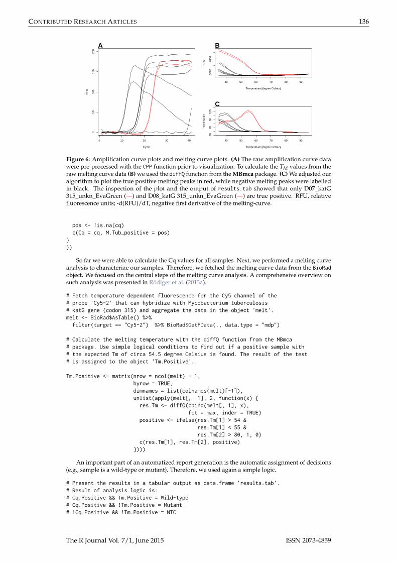
Figure 6: Amplification curve plots and melting curve plots. (A) The raw amplification curve datawere pre-processed with the CPP function prior to visualization. To calculate the TM values from theraw melting curve data (B) we used the diffQ function from the MBmca package. (C) We adjusted ouralgorithm to plot the true positive melting peaks in red, while negative melting peaks were labelledin black. The inspection of the plot and the output of results.tab showed that only D07_katG315_unkn_EvaGreen (—) and D08_katG 315_unkn_EvaGreen (—) are true positive. RFU, relativefluorescence units; -d(RFU)/dT, negative first derivative of the melting-curve.
pos <- !is.na(cq)c(Cq = cq, M.Tub_positive = pos)
}))
So far we were able to calculate the Cq values for all samples. Next, we performed a melting curveanalysis to characterize our samples. Therefore, we fetched the melting curve data from the BioRadobject. We focused on the central steps of the melting curve analysis. A comprehensive overview onsuch analysis was presented in Rödiger et al. (2013a).
# Fetch temperature dependent fluorescence for the Cy5 channel of the# probe 'Cy5-2' that can hybridize with Mycobacterium tuberculosis# katG gene (codon 315) and aggregate the data in the object 'melt'.melt <- BioRad$AsTable() %>%filter(target == "Cy5-2") %>% BioRad$GetFData(., data.type = "mdp")
# Calculate the melting temperature with the diffQ function from the MBmca# package. Use simple logical conditions to find out if a positive sample with# the expected Tm of circa 54.5 degree Celsius is found. The result of the test# is assigned to the object 'Tm.Positive'.
Tm.Positive <- matrix(nrow = ncol(melt) - 1,byrow = TRUE,dimnames = list(colnames(melt)[-1]),unlist(apply(melt[, -1], 2, function(x) {res.Tm <- diffQ(cbind(melt[, 1], x),
fct = max, inder = TRUE)positive <- ifelse(res.Tm[1] > 54 &
res.Tm[1] < 55 &res.Tm[2] > 80, 1, 0)
c(res.Tm[1], res.Tm[2], positive)})))
An important part of an automatized report generation is the automatic assignment of decisions(e.g., sample is a wild-type or mutant). Therefore, we used again a simple logic.
# Present the results in a tabular output as data.frame 'results.tab'.# Result of analysis logic is:# Cq.Positive && Tm.Positive = Wild-type# Cq.Positive && !Tm.Positive = Mutant# !Cq.Positive && !Tm.Positive = NTC
The R Journal Vol. 7/1, June 2015 ISSN 2073-4859

CONTRIBUTED RESEARCH ARTICLES 137
# !Cq.Positive && Tm.Positive = Error
results <- sapply(1:length(Cq.Positive[,1]), function(i) {if(Cq.Positive[i, 2] == 1 && Tm.Positive[i, 3] == 1)return("Wild-type")
if(Cq.Positive[i, 2] == 1 && Tm.Positive[i, 3] == 0)return("Mutant")
if(Cq.Positive[i, 2] == 0 && Tm.Positive[i, 3] == 0)return("NTC")
if(Cq.Positive[i, 2] == 0 && Tm.Positive[i, 3] == 1)return("Error")
})
We applied names of variables and factors to all the objects (e.g, Tm.Positive, Cq.Positive) andaggregated them in the object results.tab. The aim of doing this is to present the result in an easyreadable form.
results.tab <- data.frame(cbind(Cq.Positive, Tm.Positive, results))names(results.tab) <- c("Cq", "M.Tub DNA", "Tm", "Height",
"Tm positive", "Result")
results.tab[["M.Tub DNA"]] <- factor(results.tab[["M.Tub DNA"]],labels = c("Not Detected", "Detected"))
results.tab[["Tm positive"]] <- factor(results.tab[["Tm positive"]],labels = c(TRUE, FALSE))
results.tab
The results of the analysis can be invoked by the statement results.tab (not shown). Finally, weplotted and printed the output of our melting curve (Figure 6B) and melting peak (Figure 6C) analysis.
# Convert the decision from the 'results' object in a colour code:# Negative, black; Positive, red.
color <- c(Tm.Positive[, 3] + 1)
# Arrange the results of the calculations in a plot.layout(matrix(c(1, 2, 1, 3), 2, 2, byrow = TRUE))
# Use the CPP function to preporcess the amplification curve data.plot(NA, NA, xlim = c(1, 41), ylim = c(0,200), xlab = "Cycle", ylab = "RFU")mtext("A", cex = 2, side = 3, adj = 0, font = 2)lapply(2L:ncol(qPCR), function(i)lines(qPCR[, 1],
CPP(qPCR[, 1], qPCR[, i], trans = TRUE,bg.range = c(1,9))[["y.norm"]],
col = color[i - 1]))
matplot(melt[, 1], melt[, -1], type = "l", col = color,lty = 1, xlab = "Temperature [degree Celsius]", ylab = "RFU")
mtext("B", cex = 2, side = 3, adj = 0, font = 2)
plot(NA, NA, xlim = c(35, 95), ylim = c(-15, 120),xlab = "Temperature [degree Celsius]",ylab = "-d(RFU)/dT")
mtext("C", cex = 2, side = 3, adj = 0, font = 2)
invisible(lapply(2L:ncol(melt), function(i)lines(diffQ(cbind(melt[, 1], melt[, i]), verbose = TRUE,
fct = max, inder = TRUE)[["xy"]], col = color[i - 1])))
According to the analysis by MCA the samples ‘D07_katG315. . . ’ and ‘D08_katG315. . . ’ were theonly positive samples. The remaining samples appeared to be positive in the amplification plot inFigure 5 due to primer-dimer formation or sample contamination.
The R Journal Vol. 7/1, June 2015 ISSN 2073-4859
CONTRIBUTED RESEARCH ARTICLES 138
Case study three – Isothermal amplification
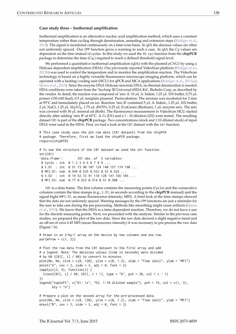
Isothermal amplification is an alternative nucleic acid amplification method, which uses a constanttemperature rather than cycling through denaturation, annealing and extension steps (Rödiger et al.,2014). The signal is monitored continuously on a time-wise basis. In qIA the abscissa values are oftennot uniformly spaced. Our CPP function gives a warning in such a case. In qIA the Cq values aredependent on the time instead of cycles. In this study we used the th.cyc function from the chipPCRpackage to determine the time (Cqt) required to reach a defined threshold signal level.
We performed a quantitative isothermal amplification (qIA) with the plasmid pCNG1 by using aHelicase dependent amplification (HDA). Our previously reported VideoScan platform (Rödiger et al.,2013b) was used to control the temperature and to monitor the amplification reaction. The VideoScantechnology is based on a highly versatile fluorescence microscope imaging platform, which can beoperated with a heating/cooling unit (HCU) for qPCR and MCA applications (Rödiger et al., 2013a,b;Spiess et al., 2015). Since the enzyme DNA Helicase unwinds DNA, no thermal denaturation is needed.HDA conditions were taken from the ‘IsoAmp III Universal tHDA Kit’, Biohelix Corp, as described bythe vendor. In detail, the reaction was composed of ‘mix A’ 10 µL A. bidest, 1.25 µL 10X buffer, 0.75 µLprimer (150 nM final), 0.5 µL template plasmid. Preincubation: The mixture was incubated for 2 minat 95°C and immediately placed on ice. Reaction ‘mix B’ contained 5 µL A. bidest., 1.25 µL 10X buffer,2 µL NaCl, 1.25 µL MgSO4, 1.75 µL dNTPs, 0.25 µL EvaGreen (Biotium), 1 µL enzyme mix. The mixwas covered with 50 µL mineral oil (Roth). The fluorescence measurement in VideoScan HCU starteddirectly after adding ‘mix B’ at 65°C. A 1x (D1) and a 1 : 10 dilution (D2) were tested. The resultingdataset C81 is part of the chipPCR package. Two concentrations (stock and 1:10 diluted stock) of inputDNA were used in the HDA. First, we had a look at the C81 dataset with the str function.
# This case study uses the qIA raw data (C81 dataset) from the chipPCR# package. Therefore, first we load the chipPCR package.require(chipPCR)
# To see the structure of the C81 dataset we used the str function.str(C81)'data.frame': 351 obs. of 5 variables:$ Cycle : int 0 1 2 3 4 5 6 7 8 9 ...$ t.D1 : int 0 51 73 90 107 124 140 157 174 190 ...$ MFI.D1: num 0.549 0.535 0.532 0.53 0.525 ...$ t.D2 : int 0 19 53 72 91 110 128 147 166 185 ...$ MFI.D2: num 0.77 0.523 0.514 0.51 0.508 ...
C81 is a data frame. The first column contains the measuring points (Cycle) and the consecutivecolumns contain the time stamps (e.g., t.D1, in seconds according to the chipPCR manual) and thesignal hight (MFI.D1, as mean fluorescence intensity; MFI). A brief look at the time stamps showedthat the data are not uniformly spaced. Warning messages by the CPP functions are just a reminder forthe user to take care during the pre-processing. Methods like smoothing might cause artifacts (Spiesset al., 2015). We know that the HDA is a time-dependent reaction. Therefore, we do not have a usefor the discrete measuring points. Next, we proceeded with the analysis. Similar to the previous casestudies, we prepared the plot of the raw data. Since the raw data showed a slight negative trend andan off-set of circa 0.45 MFI (mean fluorescence intensity) it was necessary to pre-process the raw data(Figure 7A).
# Drawn in an 2-by-1 array on the device by two columns and one row.par(mfrow = c(1, 2))
# Plot the raw data from the C81 dataset to the first array and add# a legend. Note: The abcsissa values (time in seconds) were divided# by 60 (C81[, i] / 60) to convert to minutes.plot(NA, NA, xlim = c(0, 120), ylim = c(0, 1.2), xlab = "Time (min)", ylab = "MFI")mtext("A", cex = 2, side = 3, adj = 0, font = 2)lapply(c(2, 4), function(i) {lines(C81[, i] / 60, C81[, i + 1], type = "b", pch = 20, col = i - 1)
})legend("topleft", c("D1: 1x", "D2: 1:10 diluted sample"), pch = 19, col = c(1, 3),
bty = "n")
# Prepare a plot on the second array for the pre-processed data.plot(NA, NA, xlim = c(0, 120), ylim = c(0, 1.2), xlab = "Time (min)", ylab = "MFI")mtext("B", cex = 2, side = 3, adj = 0, font = 2)
The R Journal Vol. 7/1, June 2015 ISSN 2073-4859
CONTRIBUTED RESEARCH ARTICLES 139
0 20 40 60 80 100 120
0.0
0.2
0.4
0.6
0.8
1.0
1.2
Time (min)
MF
I
A
●●●●●●●
●
●●●●●●●
●●●●●●●●●●●
●
●●
●●●●●●●●●●●●●●●●●●●●●●●●●●●●●●●●●●●●●●●●●●●●
●●●●●●●●●●●●●●●●●●●●●●●●●●●●●●●●●●●●●●●●●●●●●●●●●●●●●●●●●●●●●
●●●●●
●●●●●●●
●●●●●●●●●●●●●●●●
●
●●●●
●●●●●●●●●●●
●●●●●●●●●●●●●●●●●●●●●●●●●●●●●●●●●●●●●●●●●●●●●●●●●●●●●●●●●●●●●●●●●●●●●●●●●
●●●●●●●●●●●●
●●●●●●●●●●●●●●●●●●●●●●●●●●●●●●●●●●●●●●●●●●●●●●●●●●●●●●●●●●●●●●●●●●●●●●●●●●●●●●●●●●●●●●●●
●
●●●●●●●●●●●●●●●●●●●●●●●●●●●●●●●●●●●●●●●●●●●●●●●●●●●●●●●●●●●●●●●●●●●●●●●●●●●●●●●●●●●●●●●●●●●●●●●●●●●●●●●●●●●●●●●●●●●●●●●●●●●●●●●●●●●●●●●●●●●●●●●●●●●●●●●●●●●●●●●●●●●●●●●●●●●●●●●●●●●●●●●●●●●●●●●●●●●●●●●●●●●●●●●●●●●●●●●●●●●●●●●●●●●●●●●●●●●●●●●●●●●●●●●●●●●●●●●●●●●●●●●●●●●●●●●●●●●●●●●●●●●●●●●●●●●●●●●●●
●●●●●●●●●●●
●●●●●●●●●●●●●●●●●●●●●●●●●●●●●●●●●●●●●●●●●●
●
●
D1: 1xD2: 1:10 diluted sample
0 20 40 60 80 100 120
0.0
0.2
0.4
0.6
0.8
1.0
1.2
Time (min)
MF
I
B
●
●●●●●●●●●●
●●●●●●●
●●●●●●●●●●●●
●●
●●●●●●●●●●●●●●●●●●●●●●●●●●●●●●●●●●●●●●●●●●●●
●●●●●●●●●●●●●●●●●●●●●●●●●●●●●●●●●●●●●●●●●●
●●●●●●●●●●●●●●●●●●●●●●●●●●●
●●●●●●●●●●●●●●●●●●●
●●●
●●●●●●●●●●●●●●
●●●●●●●●●●●●●●●●●●●●●●●●●●●●●●●●●●●●●●●●●●●●●●●●●●●●●●●●●●●
●●●●●●●●●●●●●●●
●●●●●●●●●●
●●●●●●●●●●●●●●●●●●●●●●●●●●●●●●●●●●●●●●●●●●●●●●●●●●●●●●●●●●●●●●●●●●●●●●●●●●●●●●●●●●●●●●
●
●●●●●●●●●●●●●●●●●●●●●●●●●●●●●●●●●●●●●●●●●●●●●●●●●●●●●●●●●●●●●●●●●●●●●●●●●●●●●●●●●●●●●●●●●●●●●●●●●●●●●●●●●●●●●●●●●●●●●●●●●●●●●●●●●●●●●●●●●●●●●●●●●●●●●●●●●●●●●●●●●●●●●●●●●●●●●●●●●●●●●●●●●●●●●
●●●●●●●●●●●●●●●●●●●●●●●●●●●●●●●●●●●●●●●●●●●●●●●●●●●●●●●●●●●●●●●●●●●●●●●●●●●●
●●●●●●●●●●●●●●●●●●●●●●●●●●
●●●●●●●●●●●●
●●●●●●●●
●●●●●●●●●●●●●●●●●●●●●●●●●●●●●●●●●●●●●●●
●
●
D1 Cq.t: 70.18 minD2 Cq.t: 93.18 min
Figure 7: Quantitative isothermal amplification by Helicase dependent amplification (HDA). (A) Theraw data of the HDA (D1, undiluted; D2, 1 : 10 diluted) exhibit some outliers (detector artifacts), anoff-set of circa 0.5 MFI and a slight negative trend in the baseline region (0–52 minutes). (B) We used theCPP function to smooth the data with a spline function. Baselining was done with a linear regressionmodel (robust MM-estimator). Finally, we used the th.cyc function (chipPCR) to calculate the cyclethreshold time for samples D1 and D2. The threshold value was set to r = 0.05 (−−, threshold line).Cqt, required time to reach a defined threshold signal level. MFI, mean fluorescence intensity.
First, we used the CPP function to pre-process the raw data. Similar to the other case studies webaselined and smoothed the amplification curve data prior to the analysis of the of the Cqt value.However, instead of the Savitzky-Golay smoother we used a cubic spline (method = "spline") in theCPP function. In addition, outliers were automatically removed in the baseline region (Figure 7A and B).The background range was defined by bare eye to be between the 1st and 190th data point (correspond-ing to a baseline region between 0 and 52 minutes). The CPP uses a linear least squares or robust fitmethods (e.g., Rfit by Kloke and McKean 2012) to estimate the slope of the background (Rödiger et al.,in press).
# Apply the CPP functions to pro-process the raw data.1) Baseline data to zero,# 2) Smooth data with a spline, 3) Remove outliers in background range between# entry 1 and 190. Assign the results of the analysis to the object 'res'.res <- lapply(c(2, 4), function(i) {y.s <- CPP(C81[, i] / 60, C81[, i + 1],
trans = TRUE,method = "spline",bg.outliers = TRUE,bg.range = c(1, 190))
lines(C81[, i] / 60, y.s[["y.norm"]], type = "b", pch = 20, col = i - 1)# Use the th.cyc function to calculate the cycle threshold time (Cq.t).# The threshold signal level r was set to 0.05. NOTE: The function th.cyc# will give a warning in case data are not equidistant. This is intentional# to make the user aware of potential artificats due to pre-processing.paste(round(th.cyc(C81[, i] / 60, y.s[["y.norm"]], r = 0.05)[1], 2), "min")
})
# Add the cycle threshold time from the object 'res' to the plot.
abline(h = 0.05, lty = 2)legend("topleft", paste(c("D1 Cq.t: ", "D2 Cq.t: "), res), pch = 19,
col = c(1, 3), bty = "n")
The pre-processed data were subjected to the analysis of the Cqt values. It is important to note thatthe trend correction and proper baseline was a requirement for a sound calculation. We calculated Cqtvalues of 70.18 minutes and 93.18 minutes for the stock (D1) and 1:10 (D2) diluted samples, receptively.
Case study four – Digital PCR
We have developed the dpcR package for analysis and presentation of digital PCR experiments.This package can be used to build custom-made analysis pipelines and provides structures to be
The R Journal Vol. 7/1, June 2015 ISSN 2073-4859

CONTRIBUTED RESEARCH ARTICLES 140
openly extended by the scientific community. Simulations and predictions of binomial and Poissondistributions, commonly used theoretical models of dPCR, statistical data analysis methods, plottingfacilities and report generation tools are part of the package (Pabinger et al., 2014). Here, we showa case study for the dpcR package. Simulations are part in many educational curricula and greatlysupport teaching. In this case study, we mimicked an in silico experiment for a droplet digital PCRexperiment similar to Figure 1. The aim was to assess the concentration of the template sample. Inthe following we will use the expression partition as synonym for droplet. The number of positivepartitions (k), total number of partitions (n) and the size of the partition are the only data required forthe analysis. The estimate of the mean number of template molecules per partition (λ) was calculatedusing the following equation (Huggett et al., 2013):
λ = − ln (1− kn). (1)
The average partition volume in our experiment was assumed to be 5 nL. We counted n = 16800partitions in total from which k = 4601 partitions were positive. The binomial distribution of positiveand negative partitions was used to determine λ (Figure 8). Our package allows both easy estimationof a density of the parameter and calculation of confidence intervals (CI) using Wilson’s method(Brown et al., 2001) at a confidence interval level of 0.95. The true number of template molecules perpartition (λ) is likely to be included in the range of the CI (Milbury et al., 2014). The obtained meannumber of template molecules per partition multiplied by the volume of the partitions (16800 · 5 nL)constitutes the sample concentration.
# Load the dpcR package for the analysis of the digital PCR experiment.require(dpcR)
# Analysis of a digital PCR experiment. The density estimation.# In our in-silico experiment we counted in total 16800 partitions (n).# Thereof, 4601 were positive (k).k <- 4601n <- 16800(dens <- dpcr_density(k = k, n = n, average = TRUE, methods = "wilson",
conf.level = 0.95))legend("topleft", paste("k:", k,"\nn:", n))#dev.off()# Let us assume, that every partition has roughly a volume of 5 nL.# The total concentration (and its confidence interval) in molecules/ml is# (the factor 1e-6 is used for the conversion from nL to mL):dens[4:6] / 5 * 1e-6
Since we assumed a partition volume of 5 nL we have a total volume of 0.084 mL and 6.40× 10⁻⁸
(95% CI: 6.2× 10⁻⁸–6.6× 10⁻⁸) molecules/mL in the sample.
Selected functionality was implemented as an interactive shiny (Chang et al., 2015) GUI applicationto make the software accessible for users who are not fluent in R and for experts who wish to automatizeroutine tasks. Details and examples of the shiny web application framework for R can be found at http://shiny.rstudio.com/. We implemented flexible user interfaces, which run the analyses and graphicalrepresentation into interactive web applications either as service on a web server or on a local machinewithout knowledge of HTML or ECMAScript (see the dpcR manual). The interface is designed ina cascade workflow approach (Data import→ Analysis→ Output→ Export) with interactive userchoices on input data, methods and parameters using typical GUI elements such as sliders, drop-downs and text fields. An example can be found at https://michbur.shinyapps.io/dpcr_density/.This approach enables the automatized output of R objects in combined plots, tables and summaries.
Case study five – Digital PCR partition volume correction
There is an ongoing debate in the scientific community about the effect of the partition volume onthe estimated copy numbers size (Huggett et al., 2015a; Corbisier et al., 2015; Majumdar et al., 2015).Corbisier et al. (2015) showed that the partition volume is a critical parameter for the measurement ofcopy number concentrations. Their study revealed that the average droplet volume defined in theQuantaSoft software (v. 1.3.2.0, BioRad QX100 Droplet Digital PCR System) is 8 % lower than the realvolume. In consequence, results of quantifications were systematically biased between different dPCRplatforms. Case study four served as an introduction into the analysis of simulated dPCR experimentswith the dpcR package. In the next case study, number five, we used the pds_raw dataset, which wasgenerated by a BioRad QX100 Droplet Digital PCR System experiment. We re-analysed the data with
The R Journal Vol. 7/1, June 2015 ISSN 2073-4859

CONTRIBUTED RESEARCH ARTICLES 141
0.30 0.31 0.32 0.33 0.34
0.00
00.
001
0.00
20.
003
0.00
40.
005
0.00
60.
007
Number of molecules per partition
Molecules/partition
Den
sity
k: 4601 n: 16800
Figure 8: dpcr_density function from the dpcR package used for analysis of a droplet digital PCR ex-periment. From 16800 counted partitions (n) 4601 were positive (k). The chart presents the distributionof mean number of template molecules per partition (λ). n, number of total partitions; k, number ofpositive partitions.
the partition volume of 0.834 nL as proposed by Corbisier et al. (2015) and a volume of 0.90072 nL asused in the BioRad QX100 Droplet Digital PCR System.
Our experimental setup was as follows. A duplex assay was used to simultaneously detect aconstant amount of genomic DNA (theoretically 102 copies/µL) and a variable amount of plasmidDNA (10-fold serial dilution, not shown). The genomic DNA was isolated from Pseudomonas putidaKT2440 and the plasmid was pCOM10-StyA::EGFP StyB. Template DNA was heat treated at 95 °C for5 min prior to PCR. We detected in Channel 1 the genomic DNA marker ileS with FAM labelledTaqman probes and in Channel 2 the plasmid DNA marker styA with HEX labelled Taqman probes.All primer/probe sequences and experimental condiditions are described in Jahn et al. 2013, 2014 andthe manual of the dpcR package. Gating and partition clustering was taken without any modificationfrom the data output of the BioRad QX100 Droplet Digital PCR System. Each partition is representedby a dot in Figure 9. First, we had a look at the data structure of the pds_raw dataset.
# Load the dpcR package and use the pds_raw dataset for the analysis of the# digital PCR experiment.# To get an overview of the data set we used the head and summary R functions# in a chain. The output shows that the dataset contains lists of different# samples (A01 ...)
require(dpcR)
head(summary(pds_raw))
Length Class ModeA01 "3" "data.frame" "list"A02 "3" "data.frame" "list"A03 "3" "data.frame" "list"A04 "3" "data.frame" "list"B01 "3" "data.frame" "list"B02 "3" "data.frame" "list"
# Next, we used str for the element A01. The element of the list contains a data frame# with three columns. Two contain amplitude values (fluorescence intensity) and one# contains cluster results (integer values of 1 - 4).
str(pds_raw[["A01"]])'data.frame': 11964 obs. of 3 variables:$ Assay1.Amplitude: num 397 399 402 416 417 ...
The R Journal Vol. 7/1, June 2015 ISSN 2073-4859
CONTRIBUTED RESEARCH ARTICLES 142
$ Assay2.Amplitude: num 3732 3808 4007 3778 3685 ...$ Cluster : int 4 4 4 4 4 4 4 4 4 4 ...
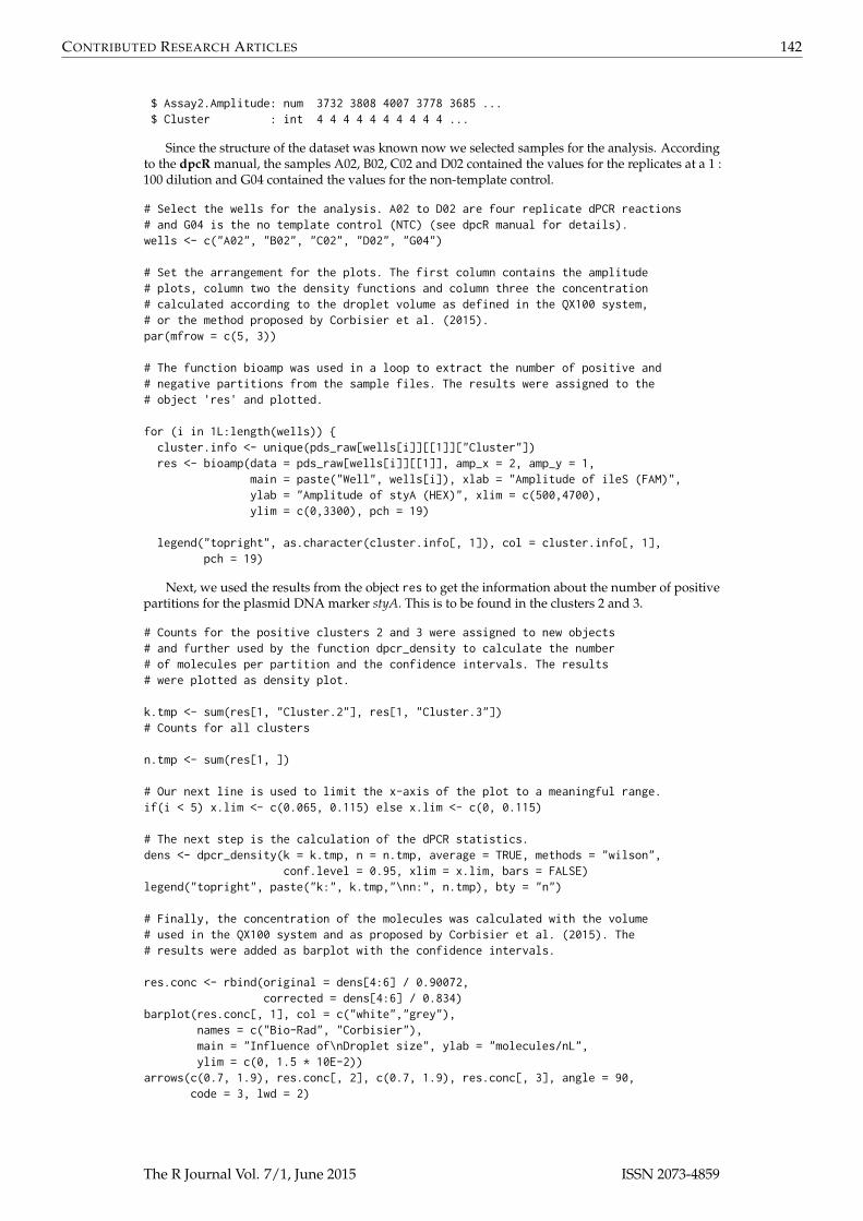
Since the structure of the dataset was known now we selected samples for the analysis. Accordingto the dpcR manual, the samples A02, B02, C02 and D02 contained the values for the replicates at a 1 :100 dilution and G04 contained the values for the non-template control.
# Select the wells for the analysis. A02 to D02 are four replicate dPCR reactions# and G04 is the no template control (NTC) (see dpcR manual for details).wells <- c("A02", "B02", "C02", "D02", "G04")
# Set the arrangement for the plots. The first column contains the amplitude# plots, column two the density functions and column three the concentration# calculated according to the droplet volume as defined in the QX100 system,# or the method proposed by Corbisier et al. (2015).par(mfrow = c(5, 3))
# The function bioamp was used in a loop to extract the number of positive and# negative partitions from the sample files. The results were assigned to the# object 'res' and plotted.
for (i in 1L:length(wells)) {cluster.info <- unique(pds_raw[wells[i]][[1]]["Cluster"])res <- bioamp(data = pds_raw[wells[i]][[1]], amp_x = 2, amp_y = 1,
main = paste("Well", wells[i]), xlab = "Amplitude of ileS (FAM)",ylab = "Amplitude of styA (HEX)", xlim = c(500,4700),ylim = c(0,3300), pch = 19)
legend("topright", as.character(cluster.info[, 1]), col = cluster.info[, 1],pch = 19)
Next, we used the results from the object res to get the information about the number of positivepartitions for the plasmid DNA marker styA. This is to be found in the clusters 2 and 3.
# Counts for the positive clusters 2 and 3 were assigned to new objects# and further used by the function dpcr_density to calculate the number# of molecules per partition and the confidence intervals. The results# were plotted as density plot.
k.tmp <- sum(res[1, "Cluster.2"], res[1, "Cluster.3"])# Counts for all clusters
n.tmp <- sum(res[1, ])
# Our next line is used to limit the x-axis of the plot to a meaningful range.if(i < 5) x.lim <- c(0.065, 0.115) else x.lim <- c(0, 0.115)
# The next step is the calculation of the dPCR statistics.dens <- dpcr_density(k = k.tmp, n = n.tmp, average = TRUE, methods = "wilson",
conf.level = 0.95, xlim = x.lim, bars = FALSE)legend("topright", paste("k:", k.tmp,"\nn:", n.tmp), bty = "n")
# Finally, the concentration of the molecules was calculated with the volume# used in the QX100 system and as proposed by Corbisier et al. (2015). The# results were added as barplot with the confidence intervals.
res.conc <- rbind(original = dens[4:6] / 0.90072,corrected = dens[4:6] / 0.834)
barplot(res.conc[, 1], col = c("white","grey"),names = c("Bio-Rad", "Corbisier"),main = "Influence of\nDroplet size", ylab = "molecules/nL",ylim = c(0, 1.5 * 10E-2))
arrows(c(0.7, 1.9), res.conc[, 2], c(0.7, 1.9), res.conc[, 3], angle = 90,code = 3, lwd = 2)
The R Journal Vol. 7/1, June 2015 ISSN 2073-4859

CONTRIBUTED RESEARCH ARTICLES 143
●●●●●●●●●●●●●●●● ●●●●●●●●●●● ●●●●●●●●●● ●●●●●●● ●●●●●●●●●●● ●●● ●●●●● ●●●●●●●●● ●●● ●●●●●● ●●●●●●●●●●● ●●●●●●●●●●●●● ●●● ●●●●●●●●●●●● ●●● ●●●●●●●●● ●●●● ●●●●●●●●●●●●●●●●●●●●●●●●●●●●●●●●●●●● ●●●●●●●●●●●● ●●●●●●●●●●●●●●●●● ●●●●●●● ●●●●●●●●●●●●●●●●●●● ●●●●●●●●● ●●●●●●●●●●●●●●●●●●●●●●●●●●●●●●● ●●●●●●●●●●●●●●●●●●●●●● ●●●●● ●●●●●●●●●●●●●●●●●●●●●●●●●●●●●●●●●● ●●●●●●●●●●●●● ● ●●● ●●●● ●●●● ●●●●●●●● ●●●●●●●●●●●● ●●●●●●●●●●●●●●●●●●●●●●● ●●●●●●●●●●●●●●●●●●●●●●●●●●●●●●●●●●●●● ●●●●● ●●●●●●●●●●●● ●●●●●●● ●●●●●●●●●●●●●●●●●●●●●●●●●●●●●●●●●●●●●● ●●●●●●●●●●●● ●● ●●●●●●●●●●●●●●●●●●●●●●●●●●● ●●●●●●●●●●●●●●●●●●●●●●●●●●●●●●●●●●●●●●●●●●●●●●●●●●●●●●●●●●●●●●●●●●●●●●●●●●●●●●●●●●●●●●●●● ●●●●●●●●●●●●●●●●●●●●●●●●● ●●●●●●●●●●●●●●●●●●●●●●●●●● ●●●●●● ●●●● ●●●●●● ●●●●●●●●●●●●●●●●●●● ●●●●●●●●●●●●●●●●●●●●●●●●●●●●●●●●●●●●●●●●●● ●●●●●●●●●●●●●●●●●●●●●●●●●●●●●●●● ●●●●● ●●●●●●●●●●●●●●●●●●●●●●●●● ●●●● ●●●●●●●●●●●●●●●●●●●●●●●●●●●●●●●●●●●●●●●●●●●●●●●●●●●●●●●●●●●●●●●●●●●●●●●●●●●●●●●●●●●●●●●●●●●●●●●●● ●●●●●●●●●●●●●●●●●●●●●●●●●●●●●●●●● ●●●●●●●●●●●●●●●●● ●●●●●● ●●●●●●●●●●●●●●●●●●●●●●●●●● ●●●●●●●●●●● ●●●● ●●●●●●●●●●●●●●●●●● ●●● ●●●●●●●●●●●●●●●●● ●●●●●●●●●●●●● ●●●●●●●●●●●●●●●● ●●●●●●●●●●●●●●●●●●●●●●●●●●●●●●●●●●●●●●●●●●● ●●●●●●●●●● ●●●●●●●●●●●●●●●●●●●●● ●●●●●●●●●●●●●●●●●●●●●●●●●●●●●●●●●●●●●●●●●● ●●●●●●●● ●●●●● ●●●●●●●●●●●●●●●● ●●●●●●●●● ●●●●●●●●●●●●●●●●●●●●●●●●●●●●●●●●●●●●●●●●●●●●●●●●●●●●●●● ●●●●●●●●●● ●●●●●●●●●●●●●●●●●●●●●●●●●●●● ●●●●●●●●●●●●●●●● ●●●●●●●●●●● ●●●●●●●●●●●●●●●● ●●●● ●●●●●● ●●●●●●●●●●●●● ●●●●●●●●●●●●● ●●●●●●●●●●●●●●●●●● ●●●●●●●●●●●●●● ●●●●●●●●●●● ●●●●●●●●●●●●●●●●●●●●●●●●●●●● ●●●●●●●●●●●●● ●●●●●●●●●●●●●●●●●●●●●●●●●●●●●●●●●●●●●●●●●●●●●●●● ●●●●●●●●●●●●●●● ●●●●●●●●● ●●●●●●●●●● ●● ●●●●●●●●● ●●●●● ●●●●●●●●●●●●●●●●●●●●●●●●●●●●●●●●●●● ●●●●●●● ●●●●●●●●●●●●●●●● ●●●●●●●●●● ●●●●●●●●●●●●●●●●●●●●●●●●●●●● ●●● ●●●● ●● ●●●●●●●●●●●●●●●●●●●●●●●●●●●●●●●●●●●●●● ●●●●● ●●●●●●●●●●●●●●● ●●●●●●●●●●●●●● ●●●●●●●● ●●●●●● ●● ●●●● ●●●●●●●●●●●●●● ●●●●●●●●●●●●●●●●●●●●●●●●●●●●●● ●●●●●●●●●●●●●●●● ●●●●●●●●●●●●●●● ●●●●● ●●●●●●●●●●●●●●●●●●●●●●●●●●●●●●●● ●●●●●●●●●●●●●●●● ●● ●●●●●●●●●●●●● ●●●●●●● ●●●●●●●●●●●●●●●●●●●●●● ●●●●●●●●●●●●●●● ●●●●●●●●●●●●●●●●●●●●●●●●●●●●●●●●●●●●●● ●●●●●● ●●●●●●●●●●●●●●●●●●●●●●●● ●●●●●●●●●●●●●●●●●●●●●●●●●● ●●●●●●●●●●●●●●●●●●●●●●●●●●●●●●●●●●●●●●●●●● ●●●●●●●●●● ●●●●●●●●●●●●●●●●● ● ●●●●●● ●●● ●●●●●●●●●●●●●●●● ●●●●●●● ●●●●●●●●●● ●●●● ●●●●●●●●●●●●●●●●●●●●●●●●●●●●●●●●●●●●●●●●●●●●●●●●●●●●●●● ●●●●●●●●●●●●●● ●●●●●●●●●●●●●●●●●●●●●●●●●●●●●●●●●●●●●●●●●●●●●●●●●●●●●●●●●●●●●●●●●●●●●●●●● ●●●●●●●●●●●●●●●●●●●●●●●●●●●●●●●●●●●●● ●● ●●●●●●●●●●●●●●●●●●●●●●●●●●●●●●●●●●●●●●●●●●●●●●●●●●●●● ●●●●● ●●●●●●●●●●●●●●●● ●●●●●●●●● ●●●●●●●●●●●●●●●●●●● ●●●●●●●●●●●●●●●●●●●●●●● ●●●● ●●●●●●●● ●●●●●●●●●●●●●●●●●●● ●●●●●● ●●●●●●●●●●●●●●●●●●●●●●●●●● ●●●●●●●●●●●●●●●●●●●●●●●●●●●●●●●●●●●●●● ●●●●●●●●●●●●●●●●●●●● ●●●●●●●●●● ●●●●●●●●●●●●●●●●●●●●●●●●●●●●●●●●●●●●●●●●●●●●●●●●●●●●●●●●●●●●●●●●●●●●●●●●●●●●●●●●●●●●●●●●●●●●●●●●●●● ●●●●● ● ●●●●●●●●●●●●● ●●●●●● ●●●●●●● ●●●●●●●●●●●●●●●●●●●●●●●●●● ●●●●●●●●●●●●●●●●●●●●●●●●●●●● ●● ●●●●●●●●●●●●●●●●●●● ●●●●●●●●●●●●●●●●●●●●●●● ●●●●●●●●●●●●●●●●●●●●●● ●●●●●●●●●●●●●●●●●●●●●●●●●●●●●●●●●●●●●●●●●●●●●●●● ●●●●●●●●●●●●●●●●●●●●●●●●●●●●●●● ●●●●●●●●●●●●●●●●●●●●●●●●●●●●●●●● ●●●●●●●●●●●●●●●●●●●●●●●●●●●●●●●●● ●●●●●●●●●●●●●●●●●● ●●●●●●●●●●●● ●●●● ●●●●●● ●● ●●●●●●●●●● ●●● ●●●●●●●●●●●●●●●●●●●●●●●●●●●●●●●●●●●●●●●●●●●●●●●●● ●●●● ●●●●●●● ●●●●●●●●●●●●●●●●●●●●●●●●●●●●●●●●●●●●●●●●●●●●●●●●●●●●●●●●●●●●●●●●●●●●●●●●●●●●●●●●●●●●●●●●●●●●●●●●●●●●●●●●●●●●●●●●●● ●●●●●●●● ●●●● ●●● ●●●●●●●●●●●●●●●●●●●●●●●●●●●●●●●●●●●●●●● ●●●● ●● ●●●●●●●●●●●●●●● ●●●●●●●●●●● ●●●●●●●●●●●●●●●●●●●●●●●●●●●●●●●●●●●●●●●●●●●●●●●●●●●●●●●●●●●●●●●●●●●●●● ●●●●●●●●●●●●●●●●●●●●●●●●●●●●●●●●●●●●●● ●●●●●●●●●●●●●●●●●●●●●●●●● ●●●●●●●●●●●●●● ●●●● ●●●●●● ●●●●●●●●●●● ●●●●●●●●●●●●●●●●● ●●●●●●●●●●●●●●●●●●●●●●●●● ●●●●●●●●● ●●●●●●●●●●●●●●●●●●●● ●●●●● ●●●●●●●● ●●●●●●●●●●● ●●●●● ●●●●●●●●●●●●●●●●●●●●●●●●●●●●●●●●●●●●●●●●●●●●●●●●●●●●●●●●●●●● ●●●●●●●●●●●●●●●●●●●●● ●●●●●●●●●●●●●●●●●●●●●●●●●●●●●●● ●● ●●●●●●●●●●●●●●●●● ●●●●●●●●●● ●●●●●●●●●●●●●●●●● ●●●●●● ●●●●●●●●●●●●●●●●●●●●●●●●●●●●●●●●● ●●●●● ●●●●●●●●●●●●●●●●●●●●●●●●●●●●●●●●●●● ●●●●●●●●●●●●●●●● ●●●●●●●● ●●●●●●●●●●●●●●●●●●● ●●●●●●●●●●●●●●●●●●●●●●●●●●●●● ●●●●●●●●● ●●●●●●●●●●●●●●●●●●●●●●●●●●●●●●●●●●●●●●●●●●●●●●●●●●●●●●●●●●●●●●●●●●●●●●●●●●●●●●●●●● ●●●●●●●●●●●●●●●●●●●●●●●● ●●●●●●●● ● ●●●●●● ●●●●●●●● ●●●●●● ●●●●●●●●●●●●●●●●●●●●●●●●●●●●●●●●●● ●●●●●●●●●●●●●●●●●●● ●●●●●●●●● ●●●●●●● ●●●●●●●●●● ●●●●●●●●● ●●●●●● ●●●●● ●●●●●●●●●●●●●●●●●●●●●●●● ●●●●●●●●●●●●●●●●●●●●●●●●●●●●●●●●●●●●● ●●●●● ●●●●●●●●●●●●●●●●● ●● ●●●●●●●●●●●●●● ●●●●●●●●●●●●●●●● ●●●●●●●●●●●● ●●●●●●● ●●●●●●●●●●●●●●●●●●●●●●●●●●●●●●● ●●●●●●●●●●●●●●●●●●●●●●●●●●●●●●●●●●●●●●●●●●●●●●●●●●●● ●●●●●●●●●●●●●●●●●●●●●●●●●●●●●●●●●●●●●●●●●●●●●●●●●●●●●● ●●●● ●●●●●●●●●●●●●●●●●●●●●●●●●●●●●●●●● ●● ●●●●●●●●●●●●●● ●●●●●●●●●● ●●●●●●●●●●●●●●●●●●● ●●●●●●●● ●●●●●●● ● ●●●●● ●●●● ●●●●●●●●●●●●●●●●●●●●● ●●●●●● ●●●●●●●●●●●●●●●●●●●●●● ●●●●●●●●●●●●●●●●●●●●●●●●●●●●●●●●●●●● ●●●●●● ●●●●●●●●●●●●●●●●●● ●●●●●●●●●●●● ●●●●●●●●●●●●●● ●●●●●●●●●● ●● ●● ●●●●●●●●●●●●●●●●●●●●●●●●●●● ●●●●●●●●●●●●●●●●●●●●●●● ●●●●●● ●●●●●●●●●●●●●● ●●●●●●●●●●●●●●● ●●●●●●●●●●●●●●●●●●●●●●● ●●●●●●●●●●●●●●●●●●●●●● ●●●●●●●●●●●●●●● ●● ●●●●●●●●●●●●●●●● ●●●●●●●●●●●●●●●●●● ● ●●● ●●●● ●●●● ●●●●●●● ●●●●●●●●●●● ●●●●● ●●●●●●●●●● ●●●●●●●●●●●●●●●●●● ●●●●●●● ●●●●●●●●●●●● ●●●●●●●●●●●●●●●●●●●●●●● ●●●●●●●●●●●●●●●●●●●●●●●●●●●●●●●●●●●●●●●●●●●●●●●●●●●●●●●● ● ●●●●●●●●●● ●●●●●●●●●●●●●●●●●●●●●●●●●●●●●●●●●●●●●●●●●●● ●●●●●●●●●●●●●●●●●●●●● ●●●●●●●●●●●●●●● ●●● ●●●●●●●●●●●●●●●●●● ●●●●● ●●●●●●●●●●● ●●●●●●●●●●●●●●●●●●●●●●●●●●●●●●●●●●●●●●●● ●●●●●●●●●●●●●●● ●●●●●●●●●●●●●●●● ●● ●●●●● ●●● ●●●●●●●●●●●●●● ●●●●●●●●●●●●●●●●●●●●●●●●●●●● ●●●●●●●●●●●●●●●●●●● ●●●●●●●● ●●●●●●●●●●●●●●● ●●●●●●●●●●●●●●●●●●●●●●●●●●● ●●●●●● ●●●●●●● ●●●●●●●●●●●●●●●●●●●●●●●●●●●●●●●● ●● ●●●●●●●●●●●●●●●●●●● ●●●●●●●●●●● ●●● ●●●●●●● ●●●●●●●●●●●●●●●●●●●●●● ●●● ●●●●●●●●●●●●●●●●●● ●● ●●●●● ●●●●●●●●●●●●●●●●●●● ●●●●●●●●●●●● ●● ●●●●●●●●●●●●●●●●●●●●●●●●●●●●●●●●● ●●●●●●●●●●●● ●●●● ●●●●●●●● ●●●●●●●●●●●●●●●●●●●●●●●● ●●● ●●●● ●●●●●●●●●●●●●●●●● ●●●●●●●●●●●●●●●●●●●●●●●●●●●●●● ●●●●●●●●●●●●●●●●●●●●●●●●●●●●●●●● ●●●●●●●●●●●●●●●●●●●● ●●●●●●● ●●●●●● ●● ●●●●●●●●●●● ●●●●●●●●●●●●●●●●●●●●●●● ●●●●●●●●●●●●● ●●●●● ●●●●●●●●●●●●●●●●●●●●●●●●●●●●●●●●●●●● ●●●●●●●●●●●●●●●●●●●●●●●●●●●●●●●●●●●●●●●●●●●● ●● ●●●●●●●●●●●●●●●●● ●●●●●●●●●●●●●●●●●●●●●●●●●●●●●●●●●●●●●●●●●●●●●●●● ●●●●●●●●●●●●● ●●● ●● ●●●●●● ●●●● ●●●●●●●●●●●● ●●●●●●●●●●●●●●●●●●●● ●●●●●● ●●●●●●●●●●●●●● ●●●●●●●●●●●●● ● ●●●● ●●●●●●●●●● ●●●●●● ●●●●●●●●●●●●●●●●●●● ●●●●●●●● ●●●●●●●●●●●●● ●●●●●●●●●●●●●●●●●●●●●●●●●●●●●●●●●●●●●●●●●●●●●●●●●●●●●●●●●●●●●●●●●●●●●●●●●●●●●●●●●●●●● ●●●●●●●●● ●●●●●●●●●● ●●●●● ●●●●●●●●●●●●●●●● ●●●●●●●●●●●●●●●●●●●●●●●●●●●●●●●●●●●●●●●●●●●●●●●●●●●●●●●●●●●●●●●●●●●●● ●●●●●●●●● ●●● ●●●● ●●●●●●●●●●●●●●●●●●●●●●●●●●● ●●●●●●●●●●●●●●●● ●●●●●●●●● ●●●●●● ●●●●●●●●● ●●●●●●●●●●●●●● ●●●●●●● ●●●●● ●●● ●●●● ●● ●●●●●●● ●●●●●●●●●●●●●●●●●● ●●●● ●●●●●●●●●●●●●●●●●●●●●●●●●●●●●●●●●●●●●●●●●●●●●●●●●●●●●●●●●●●●●●●●●●●●●●●●●●●●●●● ● ●●●●●●●●●●●●●●●● ●●●●●● ●● ●●●●●●●●●●● ●●●●●●●●●●●●●●●●●●●●●●●●●●●●●●●●●●●●● ●●●●●●●●●●●●●●●● ●●●●●●●●●●●●●●●●●●●●● ●●●● ●●●●●●●●●●●●●●●●●●●●●●●●●●●●●●● ●●●●●●●●●●●●●●●●●●●●●●● ●● ●●●●●●●●●●●●●●●●●● ●●● ●●●●● ●●●●●●● ●●●●●●●●●●●●●●●●●●●●●●●●●●●●●●●●● ●●● ●●●●●●●●●●●● ●●●●●●●●●●●●●●●●● ●● ●●●●● ●●●●●●●●●●●●●●●●●●● ●●●● ●●●●●●●●●●● ●●●●●●●●● ●●●●●●●●●●●●●●●●●●●●●●●●●●●●●●●●●●●●●●●●●●●●●●●● ●● ●●●●●●●●●●●●●●●●●●●● ●● ●●●●●●●●●●●●●● ●●●●●●●●●●●●●●● ●●●● ●●●●●●●●●●●●●●●●●●●●●●●●●●●●●●●●●●●●●●●●●●● ●●●●●●●●●●●●●●●● ●●●●●●●●● ●●●●●●●●●●●●●●●●●●●●●●●●●●●●●●●●●●●●●●●●●●●●●●●●● ●●●●●●●●●●●●●●●●● ●●●●●●●●● ●●●●●●●●●●●●●●●● ●●●●●●●●●●● ●●●●●●●●●●●●●●●●●● ●●● ●●●●●●●●●●●●●● ●●●●●●●●●●●●●●●●● ●●●●●●●●●●●●●●● ●●●●● ●●●●●●●●●●●●●● ●●●●●●●●●●●●●●●●●●●●● ●●●●●●●●●●●●●●●●●●●●●●●●●●●●●●●●●●●●●●●●●●●●●●●●●●●●●●●●●●●●●●●●●●●●●●●●● ●●●●●●●●●●●●●●●●●●●●●●●●●●●●●●●●●●●●●●●●●●●●●●●●●●●●●● ●●●●●●●●●●●●●●●●●●●●●●●●●●●●●●●●●● ●●●●●●●●● ●●●●●●● ●●●●●●●● ●● ●●●●●●●●●●●●●●●●●●●●●●●●●●●●●●●●●●●●●●●●●●●●●●●●●●●●●●●●●●●●●●●●●●●●●●● ●●●●●●●●●●● ●●●●●●●●●●●●●● ●●●●●● ●●●●●●●●●●●●●●●●●●●●●●●●●●●●●●●●●●●●●●●●●●●●●●●●●●●●●●●●●●●●●●●●●●●●●●●● ●● ●● ●●●●●●●●●●●●●●●●●●●●●●●●●●●●●●●●●●●●●●●●●●●●●●●●●●●● ●●●●●●●●● ●●●●●●●●●● ●●●●●●●●●●● ●●●● ●●●●●●●●●●● ●●●●●●●●●●●●●●●●●●●●●●●●●●●●●●● ●●●●●●●●●●●● ●●●●●●●●● ●●●●●●● ●●●● ●●●●●●●● ●●●●●●●●●● ●●●●●●●●●●●●●●● ●●●●●●●●●●●●●●●●●●●●●●●●●●●●●●●●●●●●●● ●●●●●●● ●●●●● ● ●●●●●●●●●●●●● ●● ●●●●●●●●●●●●●●●●●● ●●●●●● ●●●●●●● ●●●●●●●●●●●●●●●●●●●●●●●●●●●●● ●●●●●●●●●●●●●●●●●●● ●●●●●●●●●●●●●● ●●●●●●●●● ●● ●●●●●●●●●●●●●●●●●●●●●●●●●●●●●●● ●●●●●●●●●●●●●●●●●●●●●●●●●●●●●●●●●●●●●●●●●●●●●●●●●●●●●●●●●●●●●●●●●●●● ●●●●●●●●●●●●●●●●●●●●●●●●● ●●●●●●●●●●●● ●●●●●●●●●● ●●●●●●●●●●●●●●●●●●●●●●● ●●●●●●●●●●● ●●●●●●●●●●●●●●●●●●● ●●●● ●●●●●●●●● ●●●●●●●●●●●● ●●●●●● ●●●●●● ●●●●●●●●●●●●●●●●●●●●●●●●●●●● ●●●●●●●●●●●●●●●●●●●●●●●●●●●●●●●●●●●●●●●●●●●●●●●●●●●●●●●●●●●●●●● ●●●●●●●●●●● ●●●● ●●●●●●●●●● ●●●●●●●●● ●●●●●●●●●●●●●● ●●●●●●●●●●●●●●● ●●●●●●●●●●●●●●●●●●●●●●●●●● ●● ●● ●●●●●●●●●●●●●●●●●●●●●●●●●●●●●●● ●●●●●●●● ●● ●●●●●●●●●●●●●●●●●●●●●●●●● ●●● ●●● ●●●● ●●●●●● ●●●●●●●● ●●●●●●●●●●●●●●●●●●● ●●●●●●●● ●●●●●●● ●● ●●●●●●●●●●●●●●●●●●●●●● ●●●●●●●●● ●●●●●●●●●●●●●●●●●●●●●●●●●● ●●● ●●●●●●●●●●●●●●●● ●● ●●● ●●●●●●●●●●●●●●●●●●●●● ●●●●●●●●●●●●●●●●●●● ●●●●●●●●●●●●●●● ●●● ●●●●●● ●●●●●●●●●●●●●●●●●●●●●●●●●● ●●●●●●●●●●●●●●●●●●●●●●●●●●●●●●●●●●●●●●●●●●●●●●●●●●●●●●●●● ●● ●●● ●●●●●● ●●●●●●●●●●●●●●●●●● ●●●●●●●●●●● ●● ●●● ●●●●●●●● ●●●●●●●●●●●●●●●●●● ●●●● ●●●●●●●● ●●●●●●●●●●●●●● ●● ●●●●●●●●● ●●●●●●● ●●●●●●●●●●●●●●●●●●●●● ●●●●●●●●● ●●●●●●●●●●●●●●●●● ●●●●●●●●●●●●●●●●●●●●●●●● ●●●●●●●●●●●●●●●●●●●●●●●●●●●●●●●●●●●●●●●●●●● ●●●●●●● ●●●●●●●●●●●●●●●●● ●●●●●●●●●●●●●●●●●●●●●●●●●●●●●●●●●●●●●●●● ●●●●●●●●●●● ●●●●●●●●●●●● ●●●●●●●●● ●● ●●●●●●●●●●●●●●●●●●●●●●●●●●●●●●●●●●●●●●●●● ●●●●●●●●●●●●●●● ●●●●●●● ●● ●●●●● ●●●●●●●● ●●●● ●●●●●●●●●●●●●●●●●●●●●●●●●●●●●●●●●●● ●●● ●●●●●●●● ●●●●●●●●●●●●●●●●●● ●●●●●●●●●●● ●●●● ●●●●●●●●●●● ●●●●●●●●●●●●●●●●● ●●●●●● ● ●●●●●●●●●●●● ●●●●●●●●●●●●●●●●●●●●●●●●●●●●●●●●●●●●●●●●● ●●●●●●●● ●●●●●●●●●●●●●●●●●●●●●●●●●●●●●●●● ●●●●● ●●●●●● ●●●●●●●●●● ● ●●●●●●●●●● ●●● ●●●●●●●● ●●● ●●●●●●●●●●●●●●●●●● ●● ● ●●● ●●●●●●●●●●●●●●●●●●●●●●●●●●●●●●●●●●●● ●● ●●●●●●●●●●●●●●●●●●●●●●● ●●●●●●●●●●●●●●●●●●●●●●●●●●●●●●●●●●●● ●●●● ●●●●●●●●●●●●●●●●●●●●●●●●●●●●●●●●●●●●● ●●●●●●●●●●● ●●●●●●●●●●●●●●● ●●●●●●●●● ●●●●●●●●●●● ●●●●●●●●●●●●● ●●●●● ●●●●●●●●●●●●●●●●●●● ●●●●●●●●● ●●● ●● ● ●●●●●●●●●●●●●●●● ●●●●●●●●● ●●●●●●●●●●●●●●●●●●●●●●●●●● ●●●●●●●●● ● ●●●●●●●●●●●●●●●●●●●●●●●●●●●●●●●●●●●●● ●●●●●● ●●●●●●●●●●●● ● ●●●●●●●●●●●●●● ●● ●● ●●●● ●●●●●●●●●● ●●●● ●● ●●●●●●●●●●●●●●●●●●●●●●●● ●●●●●●●●●●●●●●● ●●●●●●●●●●●●●●●●●●●●● ●●●●●●●● ●●●●●●●●●●●●●●●●●●●● ●●●●●●●●● ●●●●●●●●● ●●●●●●●●●● ●●●●●●●●●●●●●●●●●●●●●●●●●●●●●● ●●● ●● ●●●●●●●●●●●●●●●●●●●●●●●●●●● ●●● ●●●●●● ●●●●●●●●●●●●●●●● ●●●●● ● ●●●●● ●●●●●●●●●●●●●●●●●●● ●●●●●●●●●●●●●● ●●●●●●●●●●●●●●●●●●● ●●●●●●● ●●●●●●●● ●●●●●● ●●●●●●●●●●●●●●●●●●●●●● ●● ●●●●● ●●●●● ●●●●●●●●●●●●●●●●●●●●●●●●●●●●●●●●●●●●●●●●●●●●● ●●●●●●●●●●●●●●●● ● ●●● ●●●●●●●●● ●●●●● ●●●●●●●●●●●●●●●●● ● ●●●● ●●●●●●●●●●●●●●● ●●●●●●●●●●●●● ●● ●●●●●●●● ●●●● ●●●●●●●● ●● ●● ● ●●●● ●●● ●●●●●●●●● ●●●●● ●●● ●● ●●● ●●●●●●● ●●●●●●●● ●●●●●● ●●●● ●●●●●●● ● ●● ●● ●●●●● ● ●●●●●● ●●●● ●● ●●● ●● ●● ●● ●●●●●● ●●●●●● ●●●●●●● ●●●● ● ●●●●●●●●●●●●●●●●●●
●●●● ● ●●●●●●● ●● ●● ●●●● ●●●●●● ●● ●● ● ●● ●● ●●●● ●●●●● ●●●● ●●●●● ●●●●● ●●●● ●●● ●● ●●● ● ●●●● ●●●●●●●●●● ●●●●●● ●●●●●●●●●●●●●●●●● ●●●●● ●●●●●●●●●●●●●●●●●●●●●●● ●●●●●● ●●●●●●●●●●●●●●●●●● ●●●●●●●●●●●●●●●●●●● ●●●●●●●●●●●●●●●●●●●●●●●● ●●●●●●●●●●●●●●●●●●● ●●● ●●●●●●●● ●●●●●●●●●●●●●●●●●●●●●●●●●●●● ●●●●●●●●●●●●●●●●● ●●●●●●●●●●●●●●●●●●●●●●●●●●●● ●●●●●●●●●●●●●●●●●●●●●●●●●●●●●●●●●●●●●●●●●●●●●●●●●●●●●●●●●●●●●●●●●●●●●●● ●●●●● ●●●●●●●●●●●●●●●●●●●●●●●●●●●●●●●●● ●●●●●●●●●●●●●●●●●●●●●●●●●●●●●●●●●●●●●●●●●●●●●●●●●●●●●●●●●●●●●●●●●●●●●●●●●●●●●●●●●●●●●●●●●●●●●●● ●●●●●●●●●●●●●●●●●●●●●●●●●●●●●●●●●●●●●●●●● ●●●●● ●●●●● ●●●●● ●●●●●● ●●●●● ●●●●●●●●●●●●●●●●● ●●●●●●●●●●●●●●●●●●●● ●●●●●●●●●●●●●●●●●● ●●●●●●●●●●●●●●●●●●●● ●●●●●●●●●●●●●●●●●●●●●●●● ●●●●● ●●●●●●●●●●●●●●●●●●●●●● ●●●●●●●● ●●●●●●●●●●●●●●●●●●●●●●●●●●●●●●●●●●●●●●●●●●●●●●●●●●●●●●●●●●●●●●●●●●●●●● ●●●●●●●●●●●●●●●●●●●●● ●● ●●●●●●●●●●●●●●●●●●●●●
1000 2000 3000 40000
1000
2500
Well A02
Amplitude of ileS (FAM)
Am
plitu
de o
f sty
A (
HE
X)
● ●
●
●
●
●
●
●
1423
0.07 0.08 0.09 0.10 0.11
0.00
00.
006
0.01
2
Number of molecules per partition
Molecules/partition
Den
sity
k: 830 n: 11198
Bio−Rad Corbisier
Influence ofDroplet size
mol
ecul
es/n
L
0.00
0.04
0.08
0.12
● ●●●●●●●●●●● ●●●●●●●●●●●●●●●● ●●●●●●●●●●●●●●●● ●●●●●●●●●●●●●●●●● ●●●●●●●●●●●●●●●●●● ●●●●●●●●●●●●●●●●●●●●●●●●●●●●●●●●●●●●●●●●●●●●●●●●●●●●●●●●●●● ●●●●●●●● ●●●●●●●●●●●●● ●●●●●●● ●●●●●●●●●● ●●●●●●●● ●●●●●●●●●●●●●●●●●●●● ●●●●●●●●●●●●●●●●●●●●●● ●●●●● ●●●●●●●● ●●●●●●●●●●●●●●● ●●●● ●●●●●●●●●●●●● ●● ●●●● ●●● ●●●●●●●●●●● ●●●●●● ●●●●●●●●●●●●●●●●●●●●●●●●●●●●●●●●●●●●●●●●●●●●●●●●●●●●● ●●●●●●● ●●●● ●●●● ●●●●●●●● ●●●● ● ●●●●●●●●●●●●●●●● ●●●●●●●●●●●●●● ●●●●●●●●●●●●●●●●●●●●●●●●●● ●●●●●●●●●●●●●●●●●●●●●●●●●●●●●●●●●●●●●●●●●●●●●●●●●●●●●●●●●●●●●●●●●● ●●●●●●●●●●●●●●●●●●●●●●● ●●●●●●●●●●●●●●●●●●● ●●●●●●●●●●●●●●●●●●● ●●●●●●●●●●●●●●●●●●●●● ●●●●● ●● ●●●●●●●●●●●●●●●● ●●● ●●●●●●●●●● ●●●●●●●●●●●●●●● ●●●●●●●●●●●● ●●● ●●●●●●●●●●●●●●● ●●●●●●●●●●●●●●●●● ●●●● ● ●●●●● ●●●●●●●●●●●●●●●●●●●●●●●● ●●●●●●●●●●●●●●●●●●●●● ●●●●●●●●●●●●●●●●● ●●●●●●●●●●●●●●●●●●●●●●● ●●●●●●●●●●●●●●●●●●●● ●●●●●●●●●●●●●●●●●●●●●●●●●●●● ●●●●●●●●●● ●● ●●●●●●●●●●●●● ●●●●●●●●●●●●●●●●●●●●●●●●●●●●●●●● ● ●●●●●●●● ●●●●●●●● ●●●●●●●●●●●●●●●●●●●●●●●●●●●●● ●●●●●●●●●● ●● ●●●●●●●●● ●●●●●●●●●●●●●●●●●●●●●●● ●●●●●● ●●●●●●●●●●●●●●● ●●●●●●●●●● ●●●●●● ●●● ●●●●●●●●●●●●●●●●●●●●●●●●●●●●●●●●●●●●●●●●●●●●●●●●●●●●●●●●● ●●●●●●●●●●●●●●●●● ●●●● ●●●●●●● ●●●●●●● ●● ●●●● ●●●●●●●●●●● ●●●●●●●●●●●●●●●●●●●●●●●●●●●●●●● ● ●●●●●●●●●●●●●●●●●●●●●●●●●●●●●●●●●●●●●●●● ●●●●●●●●●●●●● ●●●●●●●● ●●●●●●●●●●●●●●● ●●●●●●●●●●●●●●●●●●●●●●●●● ●●●●●●●●●●●●●●●●●●●●●●●● ●●●●●●●●●●●●●●●●●●●● ●●●●●●●●●● ●●●●●●●●● ●●●●●●●●●●●●●●●●●●●●●●● ●●●●●●●●●●●● ●●●●●●●●●●●●●● ●●●●●●● ●● ●●●●●●●●●● ●●●●●●●●●●●●●●●●● ●●● ●●●●●● ●●●●● ●●●●●●●● ●●●●●●●●●●●●●●●●●●●●●●●● ●●●●●●●●● ●●●●●● ●●●●●●●●●●●●●●●●●●●●● ●●●●●●●●●●●●●●● ●● ●●●●●●●●●●●●●●●●●●●● ●●●● ●● ●●●●●●●●●●●●●●● ●●●●●●●●●●●●●●●●●●●●●●●●●●●●●●●●●●●●●●●●●●●●●●●●●●●●●●●●●●●●●●●● ●●●●●●● ●●●●● ●●●●●●●●●●●● ●●●●●●●●●●●●●●●●●● ●●●●●●●●●●● ●●●●●●●●●●●●●●●●●●●●●●●●●●●●●●●●●●●● ●●●●●●●●●●●●●●●●●●●●●●●●●●●●●●● ●●●● ●●●●●●●● ● ●●●● ●●●●●●●●● ●●●●●●●● ●●●●●●●●●●●●●●● ●●●● ●●●●●●●●●●●●●● ●●●●●●●●● ●●●●●● ●●●●●●●●●●●●●●● ●●●●●●●● ●●●●●●●●●●● ●●● ●●● ●●●●●●●●●●●●●●●●●●●●●●●● ●●●●●●●●●●●●●●●●●●●●●●●●●●●●●●●●●●●●●●●●●●●●●●●●● ●● ●●●● ●●●●●● ●●●●● ●●●●●●●●●●●●●●●●●●●●●●●●●●● ●●●●●●● ●●●●●●●● ●●●● ●●●●●●●●● ●● ●●●●●●●●●●●●●●●●●●● ●●●●●●●●●●●●●●●●●●●●●●●●●●●●●●●●●●●●●●●●● ●●●●●●●●●●●●●● ●●●●● ●●●●●●●●●●●●●●●●●●●●● ●●●●●●●●●●●●●●●●●●●●●●●●●●●●●●●●●●●●●●● ●●●●●●●●●●● ●●●●●●●●●●●●● ●●●●●●●●●●●● ●●●●● ●●●●●●●●●●●●●●● ●●●●●●●●●●●●●●●●●●●●●●●●●●●●●●●●●●●●●●●●●●●●●●●●●●●●●●●●●●●●●●●●●●●●●●●●●●●●●●●●●●●●● ●●●●●● ●●●●●●●●●●●●●●●●●●●●● ●●●●●●●● ●●●●●●●●●●●●●●●●●●●●●●●●●●●●●●●●●●●●●●●●● ●●●●●●●●●●●●●●●●●●● ●●●●●●●●●●●● ●●●●●●●●●●●●●●●●●●●●●●●●●●●●●●●●●●●●●●●●●●●●●●●●●●●●●●●●●●●●●●●●●●●●●●●●●● ●●●●●●●●●●●●●●●●●●●●●●●●●●●●●●●● ●●● ●●●●●● ● ●●●●●●●● ●●●●●●●●●●●●● ●●●●●●●●●●●●●●● ●●●●●● ●● ● ●●●●●●●●● ●●●●●●● ●●●●●●●●●●●●●●●●●●●●●●●●●●●●●●●●●● ●●●●●●●●●●●●●●●●●●●●●●●●●●●●●●●●●●●●●●●●●●●●●●●●●● ●●●●●●●●●●●●●●●●● ●●●●●● ●●●●● ●●●●●●●●●●●●●●●●●●●●●●●●●● ●●●● ●●●●●●●●●●●●●●●●●●●●●●●●●●●●●●●●●●●●●●●●●● ●●● ●● ●●●●●●●●●●●●●●●●●●●●●●●● ●●●●●●●●●●● ●●●●●● ●●●●●●●●●● ●●●●●●●●●●●●●●●● ●●●●●●●●●●●●●●●●●●●●●●●●●●●●● ●●●●● ●●●●●●●●●●●●●●●●●●●●●●●●●●●●●●●●●●●●●●●●●●●●●●●●●●●●●●●●●●●●●●●●●●●● ●●●●●●●●●●●●●●●●●●●●●●●●●●●● ●●●●●●●●●●●●● ●●●●●●●●●●●●●●●●●● ●●●●●●●●●●●●●●●●●● ●●●●●●●●●●●●●●●●●●●●●●●●●●●●●●●● ●●●●●●●●●●●●●●●●●●●●●●●●●●●●●●●●●●●●●●●● ●●●●●●●●●●●●●●●●●●●●●●●●●●●●●●●●●●●●●●●●●●●●●●●●●●●●●●●●●●●●●●●●●●●●●● ●●●●●●●●●●●●●●●●●●●● ●●●●●●●●●●●●●●●●●● ●●●●●●●●●●●●●●●●●●●●●●●● ●●●●●●●●●●●●●●●●●● ●●●●●●●●●●●●●●●●●●●●●●●●●●●●●●●●●●●● ●● ●●●●●●●●● ●●● ● ●●●●●●●●● ●●●●●●●●●●●●●●●●●●●●●●●●●● ●●●●●●●●●●●●●●●●●●●●●●●●●●●●●●●●● ●●●●●●●●●● ●●●●●●●●●●●●●●●●●●●●●●●●●●●●●●●●●●●●● ●●●●●●● ●●●●●●●●●●●●●●●●●●●●●●●● ●●●●●●● ●●●●●●●●●●●●●●●●●●●● ●●●●●●●●●●●●●●● ●●●●●●●●●●●●●●●●●●●●●●●●●●●●●●●●●●●●●●●●●●●●●●●●●●●●●●●●●●●●●●●●●●●●●●●●●●●●●●●●●●●●●●● ●●●●●●●●● ●●●●●●●●●●●●●●●●●●●●●●●●●●●●●●●●●● ●●●●●●●●●●●●●●●●●●●●●●●●●●●●●●●●●●●●●●●●●●● ●●●●●●●●●●●●● ●●●●●●●●●●●●●●●●●●●●●●●●●●●●●●●●●●●●●●●●●●● ●●●●●●●●●● ●●●●●●●●●●● ●●●●●●●● ●●●●●●●●●●●●●●●●●●●●●●●● ●●●●●●●●●●●●●●●●●●●●●●●●●● ●●●●●●●●●● ●●●●●●●●●●●●● ●●●● ●● ●●●●●●●●●● ●●●●●●● ●●●●●●●● ●●●●●●●●●●●●●●● ●●●●●●●●●●●●●● ●●●●●●●●●●●●●●●●●●●●●●●●●●●●●●●●●●●●●●●● ●●●●●●●●●●●●●●●●●●●●●●●●●●● ●●●●●●●●●●● ●●●●●●●●●●●●●●●●●●●●●●●●● ●●●●●●●●●●●●●●●●●●●●●●●●●●●● ●●●●●●●●●●●●●●●●● ●●● ●●●●●●●●●●●●●●●●●●●●● ●●●●●●●●●●●●●●●●●●●●●● ●●●●●●● ●●●● ●●●●●●●●●●● ●●●●●●●●●●● ●●●●●●●●●●●●●● ●●●●●●●●●●●●●●●●●●●●●●●●●●● ●●●●●●●●●●●●●●●●●●●●●● ●●●●●●●●●●●●●●●●●●●●●●●●●●●●●●●●●●●●●●●●●●●●●●●●●●● ●●●●●●●●●● ●●●●●●●●●●●●● ●●●●●●●●●●●●●●●●●●●●●●●●●● ●●●●●●●●●●●●●●●●●●●●●●●●●●●●●●●●●●●●●●●●●●●●●●● ●●●●●●●●●●●●●●●●●●●●●●●●●●●●●●●●●●●●● ●●●●●●●●●●●●●●●● ●● ●●●●●●●● ●●●●●●●●●●●●●●●●●●●●●●●●●●●●●●●●●●●●●●●●●●●●●●●●●●●● ●●●●●●●●●●●●●●●●●●●●●●●●●●●●●●●● ●●●●●●●●●● ●●● ●●●●●●●●●●●●●●●● ●●●● ●●●●●●●●●●●●●●●●●●●●●●●●●●●●●●●●●●●●●●●●●●●●●●●●●●●●●●●●● ●●●●●●●●●●●●●●●●●●●●●●●●●●●●●●●●●● ●●●●●●●●●●●●●●●● ●●●●●●●●●●●●●●●●●●●●● ●●●●●●●●●●●●●●●●●●●●●●●●●●●●●●●●●●● ●●●●●●●●●●●●●●●●● ●●●●●●●●●●●●●●●●●●●●●●●●●● ●●●●●●●●●●●●●● ●●●●●●●●●●●●●●●●●●●●●●●●●●●●●●●●●●●●●●●●●●●●●●●●● ●●●●●●●●●●●●●●●●●● ●●●●●●●●●●●●●●●●●●●●●●●●●●●●●● ●● ●●●●●●●●●●●●●●●●●●● ●●●●●● ●●●●●●●●●●●●●●●●●●●●●●●●● ●●●●●●●●●●●●●●●●●●●●●●●●●●●●●●●●●●●●●●●●● ●● ●●●●●●●●●●●●●●●●●●●●●●●●●●●●●●● ●●●●●●● ●●●●●●●● ●●●●●●●●●●●●●●●●●●●●●● ●●●●●●●●●●●●●●●● ●●●●●●●●●●●●●●●●●●●●●●●●●●●●●●●●●●●●● ●●● ●●●●●●●●●●●●●● ●●●●●●●●●●●●●●●●●●●●●●●●●●●●●●●●●●●●●●●●●●●●●●●●●●●●●●●●● ●●●●●●●●●●●●●●●● ●● ●●●●●●●●●●●●●●●●●●●● ●●●●●●●●●●●● ●●●●●● ●●●● ●●●●●●●●●●●●●●●●●●● ●●●● ●● ●●●●●●●●●●●● ●●●●●●●●●●●●●●●●●●●●●●●●●●●●●●●●●●●●●●●●●●●●●●●●● ●●●●●●●●●●●●●●●●●●●●●●●● ●●● ●● ●●●●●●●●●● ●●● ●●●●●●●●●●●●●●●●●●●●●● ●●●●●●●●●●●●●●●●●●●●●●●●●●●●●●●●●●●●●●●●●●●●●●●●●●●●●●●●●●●● ●● ●●●●●●●●●●● ●●●●●●●●●●●●●●●●●●●●● ●●●●●●●●●● ●●●●●●●●●●●●●●●●●● ●●●●● ●●●●●●●●●● ●●●●●●●●●●●●●●●● ●● ●●●●●●●●●●●●●●●●●●●●●●●●●●●●●●●●●●● ●●● ●●●●●●●●●●●●●●●●●●●●●●●●● ●●●●●●●●●●●● ●●●●●●●●●●●●●●●● ●●●●●●●●●●●●●●●●●●●●●●●●●●●●●●●● ●●●●●●●●●●●●●●●●●●●●●●●● ●●●●●●●●●●●●●●●●●●●●●●● ●●●●●●●●●●●●●●●●●●●●●●● ●●●●●●●●●●●●●●●●●●●●●●●●●●●●●●●●●●● ●● ●●● ●●●●●●●●● ●●●●●●●●●●●●●●●●●●●●●●● ●●●●●●●●●●●●●●●●●●●●● ●●●●●●●●●●●●●●●● ●●●●●●●● ●●●● ●●● ●● ●●●●●●● ●●●●●●●●●●●●●●●●●●●●●●● ●●●●●●●●●●●●●●●●●●●● ● ●●●●●●●●●●●●●●●●●●● ●●●●● ●●●●●●●●●● ●●●●●●●●●●●●●●●●●●●●●●●●●●●●●●●●●●●●●●●●●●●●●●●●●●●●●●●●●●●●●●●●●●●●●●●●●●●●●●●●●●●●● ●●● ●●●●●●●● ●●●●● ●●●●●●●●●●●●●●●●●●●●●●●●●●●●●●●●●●●●●●●●●●●●●●●●● ●●●●●●●● ● ●● ●●●●●●●●●●●●●●●●●●●●●●●●●●●●●●●●● ●●●●● ●●●●●●●●●●●●●●●●●●●●●●●●●●● ●●●●●●●●●●● ●●●●●●●●●●●● ●●●●●●●●● ●●●●●●●●● ●●●●●●● ●●●● ●●●●●●●●●●●●●●●●●●●●●●●●●●●●●●●●●●●●●●●●●●●●●●●●●●●●●●●●●●●●●●●●●●●●●●●●●● ●●●●●● ●●●●●●●●●●● ●●● ●●●● ●●● ●●●●●●●●●●●●●●●●●●● ●●●●●●● ●●●●●●●●●●●●●●●●●●●●●●● ●●●●●●●●●●●●●●●●●●●●● ●●●●●●●●●●●●●●●●●●●●●●●●●●●● ●●●●●●●●●●●●●●● ●● ●●●●●● ●●●●●●●●●●●●●●●●●●●●●● ● ●●●●●●●●●●●●●●●●●●●●● ●●●●●●●●●●●●●●●●●●● ●●●●●●● ●●●●●●●●●● ●● ●●●●●●●●●●●●●●●●●●●●●●●●●●●●●●●● ●●●●●●●●●●●●●●●●●●● ●●●●●●●●●●● ●●●●●●●● ●●●●●●●●●●●●●●●●●●●●●●●●● ●●●●●●● ●●●●●●●● ●●●●●●●●●●●●●●●●●●●●●● ●●●●●●●●●●●●●●●●●●●●●●●●●● ●●●●●●●●●●●●●●●●●●●●●●●●●●●●●●● ●●●●●●●●●●●●●●●●●● ●●●●● ●● ●● ●●●● ●● ●●●●●●●●●●●●●●●●● ●●●●●● ●●●● ●●●●●● ●● ●●●●●●●●●●●●●●●●●● ●●●●●●●●●●● ●●●●● ●●●●●● ●●●●●●●●●●●●●●●●●●●●●●●●●●●●●●●●●●●●●●●●●●●●●●●●●●●●●●● ●●●●●●●●●●●●●●●● ●●●●●●●●●● ●●●●●●●●●●●●●●●●●●●●●●●●●●●●● ●●●●●●●●●●●●●●●●●●●●●●●●●●●● ●●●●●●●●●●●●●●●●●●● ●●●●●●●● ●●●●●●●●●●●●●● ●●● ●●●●●●●●●●● ●●●● ●●● ●●●●●●●●●● ●●●●●●●●●●●●●●●●● ●●●●●●●●●●●●●●●●●●●●●●●●●●●●●●●●●●●●●●● ●●●●●●●●●●●●●●●● ●●●●●●●●● ●●●●●●●●●●●●●●●●●●●●●●●●●●●●●●●●●● ●●●●● ●●●●●●●●●●●●●●●●● ●●●●● ●●●●●●●●●●●●●●●●●●●●●●● ●●●●●●●●●● ●●●●● ●●●● ●●●●●●●●●●●●●●●●●● ●●●●●●●●●●●●●●●●●●●●● ●●●●●●●●●●● ●●●●●●●●●●●●●● ●●●●●●●●●●●●●● ●●●●●●●●●●●●●●●●●●●●●●●●●●●●●●● ●● ●●●●●●●●●●●●●●●●●●●●●● ●●●●●●●●●●●●●●●● ●●● ●●● ●●●●●●●●●●●●●● ●●●●●●●●●●●●●●●●●●●●●●●●●●●●●●●●●●●●●●●●●● ●●●●●●●●●●●●●●●●●●● ●●●●●●●●●● ●●●●●●●● ●●●●● ●● ●●●● ●●●●●●●●●●●●●●●●●●●●● ●●● ●●●●●●●●●●●●●●●●●●●●●●●●●●●●●●●●●●●●●●● ●●●●●●● ●●●●●● ●●●●●●●●●●●●●●●●●●●●●●●●●●●●●●●●●●● ●●●●●●●● ●●●●●●●●●●●●● ●● ●●●●●●●● ●●● ●●●●● ●●●●●●●●●●●●●●●●●●● ●●●●●●●●●●●●●● ●●●●●●●●●●●●●●●●●● ●●●●●● ●●●●●●● ●●●●●●●●●●●●●●●●●●●●●●● ●●●●●●●●●●●●●●●●●●●●●●●●●●●●●●●●●●●●●● ●●● ●●●●●●●●●●● ●●●●●●●●●●●●● ●● ●●●●● ●●●●●●● ●●●●●●●●●●● ●●●●●●●●● ●●●●●●●●●●●●●●●●●●●●●●●●●●●●●●●●●●●●●●●●● ●●●●●●●●●●●●●●●●●●●●●●●●●●●●●●●●●●●●●●●●●●●●●●●●●●●●●●●● ●●●●●●●●●●●●● ●●●●●●●●●●● ●●●●●●●●●●● ●●●●●●●●●●●●●●●●●●●●●●● ●●●●●●●● ●● ●●●●●●●●●●●●●●●●●●●●●●●●●●●● ●●●●●●●● ●●●●● ●●●●● ●●●●●●●●●●●● ●● ●● ●●●●●● ●●●●●●●●●● ●●●●●●●●●●●●●●●●●●● ●●●●●●●●●●●●●●●●●●● ●●●●●●● ●●●●●●●●●●●●●● ●●●●●●●●●●● ●●●●●●●●●●●●●●●●●●●●●●●●●●●●●●●●●●●●●●●●●●●●●●●●● ●●●●●●●●●●● ●●●●●● ●●●●●●●●●●●●●●●●●●●●●●●●●● ●●●●●●●●●●●●●●●●●●●●●●●●●● ●●●● ●●● ●●●●●●●●●●●●●●●● ●●●●●●●● ●●●●●●●●●●●●●●●●●●●●●●●● ●●●●●●●●● ●●●●●●●●●●●●●●●●●●●●●●● ●●●● ●● ●●●● ●●●●●●●●●●●●●●●●●●●●●●●●●●●●●●●●●●●●●●●●●●●●●● ●●●●●●● ●●●●●●●●●●●● ●●●●●●●●●●●●●●●●● ●●●●●● ●●●● ●●●●●●●●● ●●●● ●●●●● ●●●●●●●●● ●●●●●●●●●● ●●●● ●●●●●●●●●●●●●● ●●●●●●●●●●●● ●●●●●●●●●●●●●●●●●●●●●●● ●●●●● ●●●●●●●●●●●●●●●●●●●●●●●●●● ●●●●●●● ●●●●●●●●●●●●●●●●●●● ●●●●●●●●●●●●●● ●●●● ●●●●●●● ●●●●●●●●●●●●●●●●●●●●●●● ●●●●●● ●●● ●●● ●● ●●●●●●●●●●●●●●●●●●●●●●●●●●●● ●●●●●●●●●● ●●●●●●●●●●● ●●●●●● ●●●●●●●●●●●●●●●●●●●●●●●●●●●●● ●●●● ●●●●●●●●●●● ●●●●●●●●●●●●●●●●●●●●●●●●●●●●●●●●●●●●●● ●●●●●●●●●●● ●●●●●●●●●●●● ●●●●●●●●● ●●●●●●●●●●●●●●●●●● ●●●●● ●●●●●●●●●●● ●●●●●●●●●●●●●● ●●●●●●●●●● ●●● ●●●●●●●●●●●●●●●●●●●●●●●●●●●●●●●●●●●●●●●●●●●●●●●●●●●●●●●●●●●●●●●●●●● ●●●●●●●●●●●●●●●●●●●● ●●●●●●●●●●●●●●●● ●●●●●●●●●●●●●●●●●●● ●●●●●●●●●●●●●●●●●●●●●●●●●●●●●●●●●●● ●●●●●●●●●●● ●●●●● ●●●●●●●●●●●●●●●●●●●●●●●●●●●● ●●●●●●●●●●● ●● ●●●●●●●●●●●●●●●●●●●●●●●●●●●●●●●●●●●●●●●●● ●●●●●●●● ●●●●●●●●●●●● ●●●●●●●●●●●●●●● ●● ●●●●●●●●●●●●●●●●●●●●●●●●●●●●●●●●●●●●●● ●●●● ●●● ●●●●●●●●●●●●●●●●●●●●●●●●●●●●●●●● ●●●●● ●●● ●●●●● ●●●●●●● ●● ●●●●●●●●●●●●●●●●●●●●●●●●●●●●●●●●●●●●●●●●●●● ●●●●●●●●●●●●● ● ●●●●●● ●●●●●●●●●●●●●●●●●●●●●●●● ●●●●●●● ●●●●● ●●●●●●●●●● ●●●●●●● ●●●●●●●●● ●●●● ●●●●●●●● ●● ●●● ●●●●●●●● ●●●●●●●●● ●●●●●●●●●● ●●●●● ●●● ●●●●●●●●●●●●●●●●●●●●●●●● ●●●●●●●● ●●●●● ●●●●●●●●●●●●●●●●●●● ●●●●● ●●●●●● ●●●●●●●●●●●●●●●●●●●●●●●●●●●●●●●● ●●●●●●●● ●● ●●●●●●●●●●●●●●●●●●●●●● ●●● ●●●●●●●●●●●●●●●●●●●●●●●●● ●●●●●●●●● ●●●●●●●●●●●●●●●●●●●●●●●●●●●●●●●●●●●●●●●●●●● ●●●●● ●●●●●●●●●●● ●●●●●●●●●●●●●●●●●●●●●●●●●●● ●●●●●●●●●●● ●●●●●●●●●●●●●●●● ●●●●●●●●●●●●●●●●●●●●●● ●●●●●●●●●●●●●●●●●●●●● ●●●●●●●●●●●●●●● ●●● ●● ●●●●●●● ●●●●●● ●●●●●●●●●● ●●●●●●●●●●●●●●●●●● ●●●●●●●● ●● ●●● ●●●●●●●●● ●●●●●● ●●●●●●● ●●●●●●●●●●●●●●●●●●●●●●●●●●●● ●●●●● ●●●●●●●●●●●●●●●●●●●●●●●●●●● ●●●●●●●●●● ●●●●●●●●●●●●●●●●●●●●●●●● ●●● ●●●●●●●●● ●●●●●●●●●●●●●●●●●●●● ●●●●●●●●●● ●●●●●●●●●●●●●●●●●●● ●●●●●●●● ●●● ●●●●●●●●●●●●●●●●●●●●● ●●● ●●●●●●●● ●●●●●●●●●●●● ●●●●●●●●●●●●● ●●●●●●● ●●●●●●●●●●●●●●●●●● ●●●●●●●●●●● ●●●●●●●●●●●● ●●●●● ●● ●●●●●●●●● ●●●●●●●●●●●●●●● ●●●●●●●●●●●● ●●●●●●●●●●●●●●●●● ●●●●●●●●●●●● ●● ●●●●●●●●●●●●●●● ● ●●●●●●● ●●●●●●●●●●●●●● ●●●●●●● ● ●●●●●●●●●●●●●●●●●● ●●●●●●●●●●●●● ●●●●●●●●●●●●● ●●●● ●●●●●●● ●●●●●●●●●●●●● ●● ●●●●●●●●●●●●●● ● ●●●●●●●● ●●●● ●●●● ● ●●●●●●● ●●●●● ●●●●●●●●● ●●●●●● ●●●●●●●●●●● ●●●●●●●● ●●●●●●●● ●●●●●●●●●●●●●●●●●●●● ●● ●●●●●●●●●●●●●●●●●●●●● ● ●●●●●●●●●●● ●●●●●●● ●●●●●●● ●●●●● ●●●●●●●●●●●●●●●●●●●●●●●●●●●●●●● ●●●●●●●●●●●●●●● ●●●●●●●●● ●●●●● ●● ●●●● ●●●●●● ●●● ●● ●●●●● ●●●●●●●●●● ●●●●● ●●●●●● ●●●●● ●● ●●●●●● ●●●●●●● ●● ●●●●●● ●●●●●●●●●● ●●●●●●●●●●●● ●● ●●●●● ●●●●●● ●● ●●●●● ●●●●●●● ●● ●● ●● ●●●●●●● ●● ●●●●●● ●● ●●●●●●●●●● ●●●● ●●●● ●● ●● ● ●● ●●●● ●●●●●● ●●●● ●●●●●● ●●●● ●●●● ●●●●●●● ● ●●●● ●●●●●●● ●● ●●●●●● ● ●●●● ●●●●● ●●● ●●●●● ●● ●●●●● ●●●● ●●● ●●●● ●●●●● ●●● ●● ● ●●● ●●● ●● ●● ●●●● ●●●● ●●●● ● ●●● ●●●● ●●●●●●● ●●●● ●● ●●● ●● ●●●●●●● ●●●●●●● ●●●● ●●●●●●●●●● ●●● ●●●●●●●●● ●●● ●●●●●●●●●●●●●●●●●●●● ●●●●●● ●●●●●●●●●●●●●●●●● ●●●●●●● ●● ●●●●●●●●●●●●●● ●●●●●●●●●●●●●●● ● ●●●●● ●●●●●●●●●●●●●●●●●●●●●●●●●●●●●●●●●● ●●●●● ●●●●●●●●●●●●●●●●●●●●●●●●●●●●●●●●●●●●●●●●●●●●●●●●●●●●●●●●●●●●●●●●●●●●●●●●●●●●●●●●●●●●●●●●●●●●●●●● ●●●●●●●●●●●●●●●●●●●●●●●●●●●●●●●●●●●●●●●●●●● ●●●●●●●●●●●●●●●●●●●●●●●● ●●●●●●●●●●●● ●●●●●●●●●●●●●●● ●●● ●●●●●●●●●●●●●●●●●●●●●●●●●●●●●●●●●●●●●●●●●●●●●●●●●●●●●●●●●●●●●●●●●●● ●●●●●●●●●●●●●●●●●●●●●●●●●●●●●●●●●●●●●●●●●●●●●●●●●●●●●●●●●●●●●●●●● ●●●●●●●●●●●●●●●●●●●●●●●●●●●●●●●●● ●●●●● ●●●●●●●●●●●●●●●●●●●●●●●●●●●●●●●●●●●●●●●●●●●●●●●●●●●●●●●●●●●●●●●●●●● ●●●●●●●●●●●●●●●●●●●●● ●●● ●● ●●●●●●●●●●●●●●●●●●●● ●●● ●●●●●●●●●●●●●●●●●●●●● ●●●●●●●●●●●●●●●●●●●●●●●●●●●● ●●●●●●●●●●●●●●●●●●●●●●●●●●●●●●●●●●●●●●●●●●●●●●●●●●●●●●●●●● ●●●●●●●●● ●●●●●●●●●●●●●●●●●●●●●●●●●●●●●●●●●●●●●● ●●●●●●●●●●●●●●●●●●●●●● ●● ●●●●●●●●●●●●●●●●●●●●●●●●●●●●●●●●●●●●●●●●●●● ●●●●●●●●● ●●● ●●●●●●● ●● ●●●●●●●●●●●●●●●●●● ●●● ●●●●●● ●●●●●●●●●●●●●●●●●●●● ●●●●●●●●●●●●●●●●●●●●●●● ●●●●
●
1000 2000 3000 4000
010
0025
00
Well B02
Amplitude of ileS (FAM)
Am
plitu
de o
f sty
A (
HE
X)
● ●
●
●
●
●
●
●
1432
0.07 0.08 0.09 0.10 0.11
0.00
00.
006
0.01
2
Number of molecules per partition
Molecules/partition
Den
sity
k: 1073 n: 11715
Bio−Rad Corbisier
Influence ofDroplet size
mol
ecul
es/n
L
0.00
0.04
0.08
0.12
●● ●● ● ●●●●●●●●● ●● ●●●●●●●●●●●●●● ●●●●●●●●●●●●●●●● ●●●● ●●●●●●●●● ●●●●●●●●● ●●●●●●●●●● ●● ●●●●● ●●●●●●● ●● ●●●●●●●● ●●●●● ●●● ●●●●● ●●●● ●●●●● ●●●●●●●●●●●●●●●●● ●●●●●●●●●●●●●●●●●●●●●●●●●●●●●●●●●● ● ●●●●●●●●●●●●●●●●●●●●●●●●●●● ●●●●●●●●●●●●●● ●●●●●●●●●●● ●●●●●●●●●●●●●●● ●●●●●●●●●●●●●●●●●● ●●●●●●●●● ●● ●●●●●●●●●●●●●●●●●●●●●●●●●●●●●●●●● ●●●●●●●● ●●●●●●●●●●●●●●●●●●●●●●●●●●●●●●●●●●●●●●●●●●●●●●●●●●●●● ●●●●●●●●●●●●●●●●●●●●●●● ●●●●●●●●●●●●●●●●●●●●●● ●●●●●●●●● ●●●●●●●●●●●●●●●●●●●● ●●●● ●●●●●●●●●●●●●● ●●●●●●●●●● ●●●●● ●●●●●●●●●●●●●●●●●●●●●●●●●●●●●●●● ●●●●●●●●●●●●●●●●●●●●●●●●●● ●●●●●●●●●●● ●●●●●● ●●●● ●●●●●● ●● ●●●●●●●●●●●●●●●●●●●●●●●●● ●●● ●●● ●●●●●●●●●● ●●● ●●●●●●●●●●●●●●●●●●●●●●●●●●●●●●●●●●●●●●●●●●●●●●●●●● ●●●●●●●●●●●●●●●●●●●●●●●●●●●●●●●●●●●●●●●●●● ●●●●● ●●●●●●●●●● ●●●●●●●●● ●●●●●●●●●●●●● ●●●●●●●●●●●●●●●●●●●●●●●● ●●●●●●●●●●●●●● ●●●●●●●●●●●●●●●●●●●●●●●●●●●●●●●●●●●●●●●●●●●●● ●●●●●●●●●●●●●●●●●●●●●●●●● ●●●●●●●●●●●●●●● ●●●●● ●●●●●●●●●●●●●●●●●●● ●●●●●●●●●●● ●●●●●●●●●●●●●●●● ●● ●●●●●●●●●●●●●●●●●●●●●●●●●●●●●●●●●●● ●●●●●●●●●●●●●●●●● ●●●●● ●●●● ●●●●●●●●●●●●●●● ●●●●●●●●●●●●● ●●●●●●● ●●●●●●●●●●●●●●●●●●●●●●●●●●●●●●●●●● ●●●●●●●●●●●●●●●●●●●●●●●● ●●●●●●●●●●●●●●●●●●● ●●●●●●●●●●●●●●●●●●●●●●●●●●●●● ●●●●●●●●●●●●● ●●●●●●●●●●●●●●●●●●●●●●●●●●●●●●●●●●●●●●●●●●●●●●●●● ●●●●●●●●●●● ●● ●●●●●●●●● ●● ●●●●●●●●●●●●●●●●●●● ●●●●● ●●●●● ●●●●●●●●●●●●●● ●●●● ●●●●●●● ●●● ●●●●●●●●● ●●●●●●●●●●●●●●●●●●●●●●●●● ● ●●●●●●●●●●●●●●●●● ●●●●●●●●●●●●●●●●●●●●●●●●●●●●●●●●●●●●●●●●●●●●●●●●●●●●●●●●●●●●●●●● ●●● ●●●●●●●●● ●●●●● ●●●●●●●●●●●●●●●●●●●●●●●●●●●●●●●●●●●●●●●●●●●●●●●●●●●●●●●●●●●●●●●●●●●● ●●● ●●●●●●●●●●●●●●●●●●●●●●●●●●●●●●●●●●●●●●●●●●●● ●●●●●●●●●●●●●●●●●●●●●●● ●●●●●●●●●●●●●●●●●●●●●● ●●●●●●●●●●●●●●●●●●●●●●●●●●● ●●●●●●●●●●●●●●●●●●●●●●●●●●●●●●●●●●●● ●●●●● ●●●●●●●●●●●●●●● ●●● ●●●●●●●●● ●●●●●●●●●●●●●●●●●●●● ●●●●●●●●●●●●●●●●●●●●●●●●●●●●●●●●●●●● ●●●●●●●●●●●●●●●●● ●●●●●●●● ●●●●●●●●●●●●●●●●●●●●●●●●●●●●● ●●●●●●●●●●●●●●●●●●●●●●●●●●●●●●●●●● ●●●●●●●●●●●●●●●●● ●●●●●●●●●●●●●●●●● ●●●●●●●●●●●●●●●●●●●●●●● ●●●●●●●●●●●●● ●●●●●●●● ●●●●●●●●●●●●●●● ●●●●●●●●●●●●●●●●●●●●●●●●●●●●●●●●●●●●●●●●● ●●●●●●● ●●●●● ●●●●●● ●●●●●●●●●● ●●●●●●●●●●●●●● ●●●●●●●●●●●●●● ● ●●●●●●●●●●●●●●●●●●●●●●●●●●●●●●●●●●●●●●●●●●●●●●●●●●●●● ●●●●●●●●●●●●●●●●●● ●●●●●●●●●●●●●●●●●●●●●●●●●●●●●●●●● ●●●●●●●●●●●●●●●●●●●●●●●●●●●●●●●●●●●● ●●●●●●●●●●●●●●●●●●●●●●●●●●● ●●●● ●●●●●●●●●●●●● ●●●●●●●●● ●●●●●●●●●●●●●●●●●●●●●●●● ●●●●●●●●●●●●●●●●●●●●●●●●●●●●●●●●●●●●●●●●●●●● ●●●●●●●●●●●●● ●●●●●●●●●●●●●●●●●●●●●●●●●●●●●●●●●●● ●●●●●●●●●●●●●●●● ●●●●●●●●●●●●●● ●● ●●●●●●●●●●● ●●●● ●●●●●●●● ●● ●●●●●●●●●●●●● ●●●●●●●●● ●●●●●● ●● ●●●●●●●●●●● ●●●●●●●●●●●●●●●● ●●●●●●● ●●● ●●●●●●●●●●●●●●●●●●●●●●●●●●●●●●●●●●●●● ●●●●●●●●●●●●●●●●●●●● ●●●●●●●●●●●●●●●●●●●●●●●●●●●●●●●●●●●●●●●● ●●●●●●● ●●●●●●●●●●●●●●●●●●●●●●●●●●●●●●●●●●●●●●●●● ●●●●●●●● ●●●●●●●●● ●●●●●●●●●●●●● ●●●●●●●●●●●●●●●●●●●●●●●●●●●●●●●●●●●●●●●●● ●●●●●●●●● ●●●●●●●●●●●●●●●●●●●●●●●●●●●●●●●●●●●●●●●●● ●●●●●●●● ●●●●● ●●●●●●●●●●●●●●● ●●●●●●●●●● ●●● ●●●●●●●●●●●●●●●●● ●●●●●●●●●●●●●●●●● ●●●●● ●●●●●●●●●●● ●●● ●●●●●●● ●●●●●●●●●●●● ●●●●●●●●●●●●●●●●●●● ●●●●●●●●● ●●●●●●●●●●●●●●●●●●●●●●●●●●●●●●●●●●●● ●●●● ●●●●● ●●●● ● ●● ●●●●●●●●●● ●●●●●●●●●●●●●●●●●●●●●●●●●●●●●●●●●●●●●●●●●●●●●●●●●●●● ●●●●●●●●●●●●●●●●●●●●●●●●●●●●●●●●●●●●●●●●●●●●●●●●●●●●●●●●●●● ●●●●●● ●●●● ●●●●●●●●● ●●●●●●●●●●●●●●●●● ●●●●●●●●● ●●●●●●●●●●●●●●●●●●●●●●●● ●●●●●●●●●●●●●●●●●●● ●●● ●●●●●●●●● ●●●●● ●●●●●●●●●●●●● ●●●●●●●●●●●●●●●● ●●●●●●●●●●●●●●●●●●●●●●●●●●●●●●●●●●●●●●●●●● ●●●● ●●●●●●●●●●●●●● ●●●●●●●●●●●●●●●●●●●●●●●●●●●●●●●●●●●●●●●●●●●● ●● ●●●● ●●●●●●●●●●●●●●●●●●●●●●●●●●●●●●●●●●●●●●●●●●●●●●●●●●●●●● ●●●●●●●●●●● ●●●●● ●● ●●●●●●● ●●●●●●●●●●●●●●●●●●●●●●●●●●●●●●●●●●●●●●●●● ●●●●●●●●●●●●●●●●●●●●●●●●●●●●●●●●●●●●●●●●●●●●●●●●●●●●●●●●●●●● ●●●●●●●●●●●●●●●●●●●●●●●●●●●●●●●●●●●● ● ●●●●●●● ●●●●●●●●●●●●●●●●●●●●● ●●●●●●●●●●●●●●●●●●●●●●●●●●● ●●●●●●●●●●●●●●●●●●●● ●●●●●●●●●●●●●●●●●●●●●●●●●●● ●●●●●●●●●●●●●●●●●●●●●●●●●●●●●● ●●●●●●●●●●●●● ●●●●●●●●● ●●●●●●●●●●●●●●●●●●● ●●●●● ●●●● ●●●●●●●●●●●●●●● ●● ●●●●●●●●● ●●●●●●●● ●●●● ●●●●● ●●●●●●●●●●●●●●●●●●●●●●●●●●● ●●●●●● ● ●●●●●●●●●●● ●●●●●●●●●● ●●●●● ●●●●●●●●●● ●●●●●●●●● ●●●●● ●●●●●●●●●● ●●●●●●●●●●●●●●●●●●●●●●●●● ●●●● ●●●●●● ●●●●●●●●●●●●●●●●●●●●●● ●● ●●●●●●●● ●●●●● ●●●●● ●●●●●● ●●● ●●●●●●●● ●●●●●●●●●●●●●●● ●●●●●●●●● ●●● ●●● ●●●●●●●●●●●●●●●●● ●●●●●●●●●●●●● ●●●●●●●●●●●●●● ●●●●●●●●●●●●●●●●●●●●●●●●●● ●●●●●●●●●●●●●●●●●●●●●●●●●●●●●●● ●●●●●●●●●●●●●●●●●●● ●●●●●●●●● ●●●●●● ●●●●●●● ●●●●●●●●●●●● ●● ●●●●●●●●●●●●● ●●●●●●●●●●●●●●●●●●●●● ●●●●●●●●● ●●●●●●●●●●●●●●●●●●●●●●●●●●●●●●●●●●●●● ●●●●● ●● ●●●●●●●●●●●●●●●●●●●●●●●●●●● ●●●●●●●●●●●●●●●●●●●●●●●●●●●●●●●●●●●●●●●●●●●●●●●●●●●●●●●●●●● ●●●●●●●●●● ●●●●●●●●●●●●●●●●●●●●●●●●●●●●●●●●●●●●●●●●●●●●● ●● ●●●●●●●●●●●●●●●●● ●●●●●●●●●●●●●●●●●●●●●●●●●●●●●●●●●●●●●●●●● ●●● ●●● ●●●●●●●●●●●●●●●●●●●● ●●●●●●●●●●●●●●●●●●●●●●●●●●● ●●●●●●●●● ●●●●● ●● ●●●●●●●●●●●●●● ●●●●●●●●●●●●●●●●●●●●●●●●●●●●●●●●● ●●●●● ●●●●●●●●●●●●●●●● ●●●●●●● ●●● ●●●●●● ●●●●●●●●●●●●●●●●●●●●●●●●●● ●●●●●●●●●●●●●●●●●●●●● ● ●●●●●●●●●●●● ●●●●●●●●●●●●●● ●●●●●●●●●●●●●●●●●●●●●●●●●●●●●●●●●●●●●●●●●●●●●●● ●●●●●●●●●●●● ● ●●●●●●●●●●● ●●● ●●●●●●●●●●●●●●●●●●●●●●●●●●●●●●●●●●●●●●●●●●●●●●●● ●●●●●●●●●●●●●●●●●●●●●●●●●●●●●●●● ●●●● ●●●●●●●●●●●●● ●●●●●●●●●●●●●●●●●●●●●● ●● ●●●● ●●●●●●●●●●●●● ● ●●●●●●●●●●● ●●●●●●●●● ●●●●●●●●● ●●●●●●●●●●●●●●●● ●●●●●●●●●●●●●●●●●●●●●●●●●● ●●●●●●●●●●●●●●●●●●●●●●●●●●●●●●●●●●●●●●● ●●●●●●●●●●●●●●●●●●●●●●● ●●●●●●● ● ●●●●●●●●●●●●●●●●● ● ●●●● ●●●●●●●●●●●●●●●●●●●● ●●●●●●●●●●●●●●●●●● ●●●●●●●●●●●●●●●●●●●● ●● ●●●●●●● ●●●●●●●●●●●●●● ●●●●●●● ●●●●●●●●●●●●●●●●●●●●●●●●●●●●●●●●●●●●●●●●●●●●●●●●● ●●●●●● ●●●●●●●●●●●●●●● ●●●●●●●●●●●●●●●●●●●●●●●●●●●●●●●●●●●●●●●●●●●●●●●●●●●●●●● ● ●●●●●●●●●●●●●●●●●●●●●●●●●● ●●●●●●●●●●●●●●●●●●●●●●●●●●●●●●●●●●●●●●●●● ●●●●●●●● ●●●●●●●●●●●●●●● ●●●●●●● ●●●●●●●●●●●●●●●●●●●●●●●●●●●●●● ●●●●● ●● ●●●●●●●●●●●●●●●●●●●●●●●●●●●●● ●●●●●●●●●●●●●●●●●●●●●●●●●●●●●●●●●●●●●●●●●●●●●●●●● ●●● ●●●●●●●●●●●●●●●●●●●●●●●●●●● ●● ●●●● ●●●●●● ●●●●●●●●●●●●●●●●●●●●●●●●●●●●●●●● ●●●●●●●●●●●●●●●● ●●●●● ●●● ●●●●●●●● ●●●●●●●● ●●●●● ●●●●●●●●●●●●●●●●●●●●●●●●●●●●●●●●●●●●●●●●●●●●●●●●●●●●●●●●●●●●●●●●● ●●●●●●●●●●●●●●●●●●●●●●● ●●●●●●● ●●●●●●●●●●●●●●●●●●● ●●●●●●●●●●●● ●●●●●●● ●●●●●●●●●●●●●●●●●●●●●●●● ●●●●●●●●●●●●●●●●●●●●●●●●●●●●●●●●●●●●●●●●●●●●●●●●●●●●●●● ●●●●●● ●●● ●●●●●●●●●●● ●●●●●●●●●●●●●●●●●●●● ●●●●●● ●●●● ●●●●●●●●●●●●●●●●●●●●●●●●●●●●●●●●●●●●●●●●●●●●●●●●● ●●●●●●●●●●●●●●●●●● ●●● ●●●●●●●●●●●●●● ●●●●●●●●●●●●●●●●● ●●●●●●●●●●●●●●●●●●●●●●●● ●●●●●●●●●●●●●●●●●●●●●●●●●●●●●●●●●●●●●●●●●●●●●●●●● ●●●●●●●●● ●●●●●●●●●●●●●●●●●●●●●●●●● ●●●● ●●●●●●●●●●●●●●●●●●●●●●●●● ●●●●●●●●●●●●●●●●●●●●●●●●●●● ●●●●●●●●●●●●●●●●●●●●●●●●●●● ●●●●●●●●●●●●● ●●●●●●● ●●●●●●● ●●●●●●●●●●●●●●● ●●●●●●●●●●●●●●●●●●● ●●● ●●●●●●●●●●●●●●●●●●●●●●●●●●●●●●● ●●●●● ●●●●●●●●●●●●●●●●● ●●●●●●●●●●● ●●● ●●●●●●●●●●●●●●●●●●●●●●● ●●●●●●● ●●●●●●●●●●●●●●●●●●●●●●●●●●● ●●●●●●●●●●●●●●●●●●●●●●● ●●●●●●● ●●●●●●●●●●●●●●●●●●●●●●●●●●●●●●●●●●●●●●●●● ●●●●●●●●●●●●●●●●●●●●●●●● ●●●●●●●●●●●●●●●●●●●●●●●●●●●●●●●●●●● ●●●● ●●●●●●●●● ●●●●●●●●●●● ●●●●●●●●●●●●●●●●●●●●●●●●●●●●●●●●●●● ●●●●●● ●●● ●●●●●●●● ●●●●●● ●●●●●●●●●●●●● ●●●●●●●●●●●●●●●●●●●●●●●●●●●●●●●●●●●●●●●● ●●●●● ●●● ●●● ●●●●●●●●●●●●●●●●●●●●●●●●●●●●●●●●●●●●●●●●●●●●●●●●●●●●●●●●●●● ●●●●●●●●●●●●● ●●●●●●●● ●●●●●●●●●●●●●●●●●●●●●●●●●●●●●●●●● ●●●●●●●●●●●●●●●●●●●●●●●●●●●●●●●●●●●●●●●●●●● ●●●●●●●●●●●●●●●●●●● ● ●●●●●●●●●● ●●●●●●●●●●●●●●●●●●●●●● ●●●● ●●●●● ●●● ●●●●●●●●● ● ●●●●●● ●●●●●●●●●●●●●●●●●●●●● ●● ●●●●●● ●●●●●●●●● ●●●●●●● ●●●●●●●●●●●●●●●●● ●●●●●●● ●●● ●●●●●●●●●●●●●●●●●●●●●●● ●● ●●●●●●●●●●●●●● ●● ●●●●●●●●●●●● ●●●● ●●●●●●●●●●●●●●●●●● ●●●●●●●●●●●●●●●●●●●●● ●● ●●●●●●●●●●●●●●●●●●●●●●●●●● ●●●●● ●●●●●●●●●●●●●●●●●●●●●● ●●●●●●●●●●●●●●●●●●●●●●●● ●●●●●●● ●●●●●●●●●●●●●●●●●●●●●●●●●●●●●●●●●●●●●●●●●●●●●●● ●● ●●●●● ●●●●●● ●●● ●●●●●●●●●●●●●●● ●●●●●●●●●●●●●● ●● ●●●●●●●●●●●●●●●●●● ●●●●●●●● ●●●●●●●●●● ●●●●●●●●● ●●●●●●● ●●●●●●●● ●●●●●●●● ●●●●●●● ●●●●●●●●●●●● ●●●●●●●●●●●●●●●●●●●●●●●●●● ●●●●●● ●●●● ●● ●●●●●●●●●●● ●●●●●●●●●●●●●●● ●●●●●●●●●●●●●●●●●●●●●●●●●●●●●● ●●● ●●●●●●●●●● ●●●●●●●●●●●●●●●●●●●●●●●●●●●●● ●●●●●●●●●●● ●●●●●●●●●●●●●●●●●●●●●●●●●●●● ●●●●●● ●●●●●●●● ●●●●●●●●●●●●●●●●●●● ●●●●●●●●●●●●●●●●● ● ●●●●●●● ●●●●●●●●●●● ● ●●●●●●●●●●●● ●●●●●●●●●●●●●● ●●●●●●●●●●●●●●●●●●●●●● ●●●●● ●●● ●●●●● ●●●●●●●●● ●●●●●●●●●●●●●●●●●●●●●●●●●●●●●●●● ●●●●●●●●●●●● ●●●●●●●●●●●●●●●●●●●●●● ●●●●●●●●●●●● ●●●●●●●●●●●●●●●●●●●●●●●●●●●●●●●●●●●●●●●●●●●●●●●●●●●● ●● ●●●●●●●●●●● ●●●●●●●● ●●●●●●●●●●●●●●●●●●●●●●●● ●● ●●●●●●●●●●●●●● ●●●●●●●● ●●●● ●● ●● ●●●●●● ●●●●●●●●●●●●●●●●●●●●●●●●●●●●●●●●●●●●●●●●●●●●●●●● ●●●●●●●●●●●●●●●●●●●●●●●● ●●●●● ●●●● ●●●●●●●●●●● ●●●●●●●●● ●●●●●●●●●●●● ●●●●●● ●●●● ●●●●●●●●● ●●●●●●●●●●●●● ●●●●●●●● ●●●●●●●●●●●●●●●●●●●●●●●●●●●●●●● ●●●●● ●●●●●●●●●●●●● ●●●●●●●● ●●●●● ●●●●●●●●●●●●● ●●●●●●●●●●●●●●●●● ●●● ●● ●●●●●●●●●●● ●●● ●●●●●●●●●● ●●●●●●●● ●●●●●●●●●●●●●● ●●● ●● ●●●●●●●●●●●●●●●●●●●●●●●●●●● ●●●●●●●●●●●●●●●●● ●●●●●●●●●●●●●● ●●● ●●●●●●●●●● ●●●●●●●●● ● ●●●●●●●●●●●●●●●●●●●● ●●●●● ●●●●●●●●●●●●●●●●●●●●●● ●●●●●●●●●●●●●●●●●● ●●● ●●●●● ●●●●●●●●●●●●●●●● ●●●●●●●● ●●●● ●● ●●●●●●●●●●●●●●●● ●●●● ● ●●● ●●●●●●●●● ●● ●●●●●●●●●●●●●● ●●●●●●●●●●●●● ●●●●●●●●●●●●●●●●●● ●●● ●●●●●●● ●●●●●●●●●●●●●●● ●●●●●●●●●●●●●●●●●●●●●●●● ●●●●●●●●●●●●●●●●●●● ●● ●●●●●●●●●●●●●●●●●●●● ●●●●●●● ●●●●●●●●●● ●● ●●● ●●●●●●●●●●●● ●● ●●● ●● ●●●● ●●●●● ●●●●●●●●●●●●● ●●●●●●●●●● ●●●●●●●●●●●●●●●●●●● ●●●●●●●●●●●●●●●●● ●●● ●●●●● ●●●●●●● ●● ●●●●● ●●●●●●●●●●●●●●●●●● ● ●●● ●●●●●● ●●●●●●●●●●●●●●●●●●●●● ●●●●●●●●●●●● ●●●●●●●● ●●●● ●●● ●● ●●●●●●●●●●●●●●● ●●●●●●●●●●●●●● ●● ●●●●●●●●● ●●●●●●●●●● ●●●●● ●●●● ●●●●●●●●● ●●●●● ●● ●●● ●●●●●● ●●● ●●●●●●●●●●● ●●●●●●●●●●● ●●●● ● ●●● ●● ●● ●●● ●●●● ●●●●●●●● ●●● ●● ●●● ●● ●●●●●●● ● ●● ● ●●●● ●● ●●●● ●● ●● ●● ●●● ●●●● ●● ●● ●●●● ●●●● ● ● ●●● ●● ●●●● ●● ●● ●●● ●●● ●●●●●● ●● ●●● ●●● ●●●● ●●●●●●●● ●●●●●●●●●●●●● ●●●●●●● ●●●●●●●●●●●●●●●●●●● ●●●●●● ●● ●● ●●●●●●●●●●●●●●●● ●●●●●●●●●●●●● ●●●●●●●●●●●● ●●●●●●● ●●●●●●●●●●●●●●●●●●●●●●●●●●●●●●●●● ●●●● ●●●●●●●●●●●● ●●●●●●●●●●●●● ●●●●●●●●●●●●●●●●●●●●●●●●●●●●●●●●●● ●●●●●●●●●●●●●●●●●●●●●●●●●●●●●●●●●●●●●●●● ●●●●●●●●●●●●●●●●●●●●● ●●●● ●●●●●●●●●● ●●●●●●●●● ●●● ●●●●●●●●●●●●●●●●●●●●●●●●●●●●●●●●●●●●●●●●●●●●●●●●●●● ●●●●●●●●●●●●●●●●●●●●●●●●●●●●●●●●●●●●●●●●●●●●●●●●●●●● ●●●●●●●●●●●● ●●●●●●●●●●●●●●●●●●●●●●●●●●●●●●●●●●● ●●●●●●●●●●●●●●●●●●●●●●●●●●●●●●●●●●●●●●●●●●●●●●●●●●●● ●●●●●●●●●●●●●●●●●●●●●●●●●●●●●●●●●●●●●●●●●●●●●●●●●●●●●●●●●●●●●●●●●●●●●● ●●●●● ●●●●●●●●●●●●●●●●●●●●●●●●●●●●●●●●●●●●●●●●●●●●●●●●●●●●●●●●●●●●●●●●●●●●●●●●●●●●●●●●●●●●● ●●●●●●●●●● ●●●● ●● ●●●●●●●●● ●●●●●●●●●●●●●●●●●●●●●●●●●●●●●●●●●●●●●●●●●●●●●● ●●●●●●●●●●● ●●●●●●●●●●●●●● ●●●●●●●● ●●●●●●●●●●●●●●●●●●●●●●●●●●●●●●●●●●●●●●● ●●●●●●●●●●●●●● ●●●●●●●●●●● ●●●●●●●●● ●●●●●●●●●●●●●●
1000 2000 3000 4000
010
0025
00
Well C02
Amplitude of ileS (FAM)
Am
plitu
de o
f sty
A (
HE
X)
● ●
●
●
●
●
●
●
1423
0.07 0.08 0.09 0.10 0.11
0.00
00.
006
0.01
2
Number of molecules per partition
Molecules/partition
Den
sity
k: 917 n: 9638
Bio−Rad Corbisier
Influence ofDroplet size
mol
ecul
es/n
L
0.00
0.04
0.08
0.12
●●●● ●● ●●● ●●●●●●●●●●●●●●●●●●●●●●●●●●●●●●●●●●●●●●●●● ● ●●● ●●●●●●● ●●● ●●●●●●●● ●●●●●●●●●●●●●● ●●●●●●●●●●●●●●● ●●●●●●●●●●●●●●●● ●●●●●●● ●●●●●●● ●●●●●●●●●●●●●●● ●●●● ●●●●●●●●● ●●●●● ●●●●●●●●●● ●●●● ●●● ●●●●●●●●●●●●● ●●●●●●●●●●●●●●●● ●●●●● ●●●●●● ●●●●●●●●●●●●● ●●●●●● ●● ●●●● ●●●●● ●●● ●●●●●●●●●●●●●●●●●●●●●●●●●●●●●●●●●●●● ●●● ●●●●● ●●●●●●●●●●●●●●● ●●●●●●●●●●●●● ●●●●●●●●●●●●●●●● ●●●●● ●●●●●●●● ●●●●●●●●●● ●●●●● ●●●●●●●●●● ●●●●●●●●●●●●●●●●●●●●●●● ●●●●●●●●●● ●●● ●●●●●●●●●●●●●● ●●●●●●●●●●●●●●●●●●●●●●●●●●●● ●●●●●● ●●●●● ●●●●●●●●●●●●● ●●●●●●●●●●●●●●●●●●●●●●●●● ●●●●●●●●●●●●●●●●●●●●●●●●●●●●●●●●●●●●●●●●●●●●●●●●●●●●●●●●●●●●●● ●●●●●●●●●●●●●●●●●●●●●●●●●●●●●●●●●●●● ●●●● ●●●●●●●●●● ●● ●●●●●●●● ●●●● ●●●●●●●●●●●●●●●●●●●●●●●●●●●●●●●●●●●●●●●●●●●●●●●●●●●●●●●●●●●●●●●●●●●●●●●●●●● ●●● ●●●● ●●●●●● ●●●●●● ●●●●●●●●●●●●●●●●●●●●● ●●●●●●●●●●●●●●●●●●●●●●● ●●●●●●●●●●●●●●●●●●●●●●●●●●●● ●●●●●●●●●●●●●●●●●●●●●●●●●●●●●●●●●●●●●●●●●●●●●●●●●●●●●●●●●●●●●●●●●●● ●● ●● ●●●●●●●●●●●●● ●●●●●●● ●●●●●●●●●●● ●●●●●●●●●●●●●●●●●●●●● ●●●●●● ●●●●●●●●●●●● ●● ●●●●●●●●●●●● ●●●●●●●●●●●●●●●●● ●●●●● ● ●●●●●●●●●●●●●●●● ●● ●●●●●●●●●●●●●●●● ●●●●●● ●●●●●●●●●●●●●● ●● ●●●●●●●●●●●●●●●●●●●●●●●●●● ●●●●●●●●●●●●●●●●●●●● ●●●●●●●●● ●●●●●●●● ●●●●●● ●●●●●●●●●●● ●●●●●●●●●●●● ●●●●● ●●●●●●●●●●●●●●● ●●●●●●●●●●●● ●●●●●●●●●●●●●●●●●●●●●●●● ●●●●●●●●●● ●●●●●●●●●●●●●●● ●●●●●●●●●●●●●●● ●●●●●●●●●●●●●●●●●●●●●●●●●●●●●●●●●●●●●●●●● ●●●●●●●●●●●●●●●●●●●●●●●●●●●● ●●●●●●●●●●●●●●●●●●●●●●●●●● ●●●●●●●●●●●●●●●●●●●●●●●●●●●●●●●●●●●●●●●●●●●●●●●●●●●●●●●●●●●●●●●●●●●●●●●●●●●●●●●●●●●●●●●●●●●●●●●● ●●●●●●●●●●●●●● ●●●●● ●●●● ●●●●●●●●●●●●●●●●●●●●●●●●●●●●●●●●●●● ●● ●●●●●●●●●●●● ●●●●●●●●●●●●●●●●●●●●●●●●●●●●●●●● ●●●●●●●● ●●●●●●●●●● ●●●●●● ●●●●●●●●●●●●●●● ●●●●●● ●● ●●●●●●●●●●●●●●●● ●●●●●●●●●●●●●●●●●●●●●● ●●●●●●●● ●●●●●●●●● ●● ●●●●●●●●●● ●●●●●●●●●●●●●● ●●●●●●●●●●●●●●●●● ●●●●●●●●●●●●●●●●●●●●●●● ●●●●●●●●●●● ●●●●●●●●●●●●● ●●●●●●●●● ●●●●●●●●●●●●● ●●●●●●●●●●●●●●●●●●●●●●●●●●●●●●●●●●●●●●●● ●●●●●●●●●●●●●●● ●●●●● ●●●●●●●●●●●●●●●● ●●●●●● ●●● ●●●●●●●●●● ●●●● ●●●●●●●●●●●●●●●●●●●● ●●●●●●●●●●●●●●●●●●●●●●●●●●●●●●●●●●●●●●●●●●●● ●●●●●●●●●●●●●● ●●●●●●●●●●●●●●●●●●●●●●●●●●●●●●●●●●●●●●●●●●●●●●●●●●●●●●●●●●●●●●●●●●●●●●●●●●●●●●●●●●●●●●● ●●● ●●●●●●●●●●●●●●●●●●●●●●●●●●●●●●●●●●●●●●●●●●●●●●●●●●●●●● ●● ●●●●●●●●●●●●●●●●●●●●●●●●●●●●●●●●●●●●●●●●●●●●●●●●●●●●●●●●●●●●●●●●●●●● ●●●●●●● ●●●●●●●●●●●●●●●●●●●●●●●● ●●●●●●● ●●●●●●●●●●●●●●●●●●● ●●●●●●●●●●●●●●●●●● ●●●●● ●●●●●●●●●●●●●●●●●●●●●● ●●●●●●●●●●●●●●●●●●●●●●●●●●●● ●●●●●●●●●●●●●●●●●●●●●●●●●● ●●●●●●● ●●●● ●●●●●● ●●●●●●●●●●●●●●●●● ●●●●●●●●●●● ●●●●●●●●● ●●●●●●●● ●●●●●●●●●●●● ●●●●●●●●● ●●●●●●●●●●●●●●●●●●●●●●●●●●●●●●●●●●●●● ●●●●● ●●●●●●●●●●●●●●●● ●●●●●●●●●●●●●●●●●●●●●●●●●●●●●●●●●●●●●●●●●●●●●●●●●●●● ●●●●●●●●●●●●●● ●●●●●●●●●●●●●●●●●●● ●●●●●●●●●●●●●●●●● ●●●●●●●●●●●●●●●●●●●●●●●●●●●●●●●●●●●●●●●●●●●●●●●●●●●● ●●●●●●●●● ●● ●●●●●●●●●●●●●●●●●●●●●●●●●●●●●●● ●●●●● ●●●●● ●●●●●●●●●●●●●●●●●●●●●●●●●●●●●●●●●●●●●● ●●●●●●● ●●●●●●●●●●●●●●●●●●●●●●●●●●●● ●●●●●●●● ●●●● ●● ●●●●●●●●●● ●●●●●●●●●●●● ●●●●●●●●●●●●●●●●●●●●●●●●●●●●●●●●●●● ●●●●●●●●●●●●●●●●●●●●●●●●●●●●●●●●●●●●●●●●●●●●●●●●●●●●●●●●●●●●●●● ●●●●●●●●●● ●●●●●●●●●●●●●●●●●●●●●●●●●●●●●● ●●●●●●●●● ●●●●●●●●●●●●●●●●●●●●●●●●●●●●● ● ●●●●●●●●●●●●●●●● ●●●●●●●●●●●●●●●●●●●●●●●●●●● ●●●●●●●●●●●●●●● ●●●●●●●●●●●●●●●●●●●●●●●●●● ●●●●● ●●●●●●●●●●●●●●●●●● ●●●●●●●●●●●●●● ●● ●●●●●●●●●●●●●●●●●●●●●●● ●●●●●●●●●●●●●●●●●●●● ●●●●●●●●●●●●●●●●●●●●●●●●●●●●●●●●●●●●●●●●●●● ● ●●●●●●●●●●●●●●●●●●●●● ●●●●●●●●●● ●●●●●●●●●●●●●●●● ●●●●●●●●●●●●● ●●●●●●●●●●●●● ●●●●●●●●●●●●●●●●●●●●●●●●●●●●●●●●●●●●●●●●●●●●●●●●● ●●●●●●●●●●●●●● ●●●●●●●●●●●●●●●●●●●●●●●●●●●●●●●●●●●●●●●● ●●●●●●●●●●●●●●●●●●●● ●●●●●●●●●●●●●●●● ●●●●●●●●●●●●●●●●●●●●●●●●●●●●●●●●●●●●●●●●●●●●●●●●●●●●● ●●●●●●●●●●●●●●●●●●●●●●●● ●●●●●●●●●●●●●●●●●●● ●●●●●●●●●●●●●●●●●●●●●●●●●●●●●●●●●●●● ●●● ●●●●●●● ●●●●●●●●●●●●●●●●●●●● ●●●●●●●●●●●●●●●●●●●●●● ●●●●●●●●●●●●●●●● ●●●●●●●●●●●●●●●●●●●●●●●●●●● ●●●●●●●●●●●●●●●●●●●●●●●●●●● ●●●●●●●●● ●●●●●●●●●●●●●●●●●●●●●●●●●●●● ●●●●●●●●●●●●●●●●●●●●●●●●●●●●●●●●●●●●●●●●● ●●●●●●●● ●●●●●●●●●●●●●●●●●● ●●●●● ●●●●●●●●●●●●●●●●●● ●●●●●●●● ●●●●●●●●●●●●● ●●●●●●●●●●●●●●●●●●●●●●●●●●●●●●●● ●●●●●●●●●●●●●●●●●●●●●●●●●●● ●●●●●●●● ●●●●●●●●●●●●●●● ●●●●●●● ●●●●●●●● ● ●●●●●●●●●●●●● ●●● ●●● ●●●●●●●●●●●●● ●● ●●●●●●●●●●●●●●● ●●●●●●●●●●●●●●●●●●●●● ●●●● ●●●●●●●●●● ●●●●●●●●●●●●●●●●● ●●●●●●●●●●●●●●● ●● ●●●●●●●●●●●●●●●●● ●●● ●●●● ●●●●●●●●●●●●●●●●●● ●●● ●●●●●●●●●●●●●●●●●● ●●● ●●●●●●●●●●●● ●●●●●●●●●●●●●●●●●●●● ●●●●● ●●●●●●●●●●●● ●●●●● ●●●●●●●●●●●●●●● ●●●●●●●●●●●●●●●● ●● ●●●●● ●●●●●● ●●●●●●●●● ●●●●●●●●●●●●●●●●●●●●●●●●●●●●●●●●●●●●●●●●●●●●●●● ●● ●●●●●●●●●●●●●●●●●●●●●●●●●●●●●● ●●●●●●●●●●●●●●●●●●●●●●●●● ●●●●●●●●●●●●●●●●●●●●●●●●●●●●●●●●●●●●●●●●●●●●●●●●●●●●●●●●●●●●●●●●●●●●●●●●●●●●●●●●●●●●● ●● ●●● ●●●●●●●●●●●●●● ●●●●●●● ●●●●●●●●●●●●●●●● ●● ●●●●●●●●●●● ●● ●●●●●●●●●●●●●● ●●●●●●●●●●●●●●●●●● ●●●●●●●●●●●●●●●●●●● ●●● ●●●●●●●●●●●●●●●●●●●●●●●●● ●●●●●●●●●●●●●●●●●●●●●●●●●●●●●●●●●●●● ●●●●●●●●● ●●● ●●●●●●●●● ●●●●●●●●●● ●●●●●●●● ●● ●●●●●●●●●●●● ●● ●●●●●●●●●●●●●●●● ●●●●●●●●●● ●●●●●●●●●●●●●●●●● ●●●●●●●●●●●●●●●●●●●●●●●●●●●●●●●●●●●●●●●●●●●●●●●● ● ●●●●●●●● ●●●●●●●●●●●●●●●●●●●●●●● ●●●●● ●●●●●●●●●●●●●●●●●●●●●●●●●●●●●●● ●●●●●●●●●●●●●●●●●●●●●●●●●●●●● ●●●●●●●● ●●●●●●●●●●●●●●●●●●●●●●●●●●●●● ●●●●● ●●●●●●●●● ●●●●●●●● ●●●●●●●●●●●●●●●● ●●●● ●●●●●●●●●●●●●●●●●●●●●●●●●●●●●●● ●●●●●● ●●●●●●●●●●●●●●●●● ●●●●●●●●●● ●●●●●●● ●●●●●●●●●●●●●●●●●●●●●●●●●●●●●●●●●●●●●●●●●●●●●●●●●●●●● ●●●●●●●●●●●●●● ●●●● ●●●●●●●●●●●●●●●●●●●●●●●●● ●●●●●●●●●●●●●●●●●●●●●●●●●●● ●●● ●●●●●●●●●●●●●●●● ●●●●●●●●●●●●●●● ●●●●●●●●●●●●●● ●●●●●●●●●●●●●●●●●●●●●●●●●●●●●●●●●●●●●● ●●●●●●●● ●●●●●●●●●●●●●●●●●●●●●●●●●●●●●●●●●●●●●●●●●●●●●●● ●●●●●●●●●●●●●●●●●●●●●●●●●●●●●●●●●●●●●●●●●● ●●●●● ●●●●●● ●●●●●●●●●●●●●●●●●●●●●●●●●●●●●●●●●●●●●●●●●●●● ●●●●●●●● ●●●● ●●●●●●●●●●●●●●●●●●●● ●●●●●●● ●●●●●●●●●●●●●●●●●●●●●●●●●●●●●●●●●●●●●●●●●●●●●●●●●●●●●●●●●●●●●●●●●●●●●●●●●●●●●●●●● ●●●●●●● ●●●●●●●●●●●●●●●●●●●●●●●●●●●●●●●●●●●●●●●●●●●●●●●●●●●●●●● ●●●●●●● ●●●●●●●●●●●●●●●●●●●●●●●●●●●●● ●●●●●●●●● ●●● ●● ●●●● ●●●●●●●●●●●●●● ●●●●●●● ●●●● ●●●●●● ●●●●●● ●● ●●●●●●●●●●●●●●●●●●●●●●●●●●●●●●●●●●●●●●●●●●●●●●●●● ●●● ●●●●●●●●●●●●●●●●●●●●●●●●●●●●●●●● ●●●●●●● ●●●●●●●●●●●●●● ●●●●●●●●●●●●●●●●●●●●● ●●●●●●●●●●●●●●●●● ●●●●●●●● ●●●●●●●●● ●●● ●●●●●●●● ●●●●●●● ●●●●●●●●●●●●● ●●●●●●●●●●●●●●●●●●●●●●●●●●●●●● ●●●●●●●●●●●●●●● ●●●●●●●●●●●● ●●●●●●●●● ●●●●●● ●●●●●●●●●●●●●●●●●●●●●●●● ●●●●●●● ●●●●●●●● ●●●●●●●●●●●●●●●●●●●●●●●●●●●●●●●●●● ●●●●●●●●● ●●●●●●●●●●●●●●●●●●●●●● ●●●●●●●●●●●●●● ●● ●●●●●●●●●●●●●●●●●●●●●●●●●●●●●●●●●●●●●●●●●●●●●●● ●●●●●●● ●●●●● ●●●●●●●●●●●●●●●●●●●● ●●●●●●●●●●● ●●●●●● ●●●●●●●●●●●●●●● ●●●●●●●●●●●●●●●● ●●●●●●●●●●●●●●●● ●●●●●●●●●●●●●●● ●●●● ●●● ●●●●●●●●●●●●●●●●●●●●●●●●●●●●●●● ●●●●●●●●●● ●●●●●●●●●●● ●●●●●●●●●●● ●●●●●●●●●●●●●● ●●●●●●●● ●●●●●●●●●●●● ●●●●●●●●●●●●●●●●●●●●●●●●●●●●●● ●●●●●●●● ●●●●●●● ●●●● ●●●●● ●●●●●●●●●●●●●●●●● ●●●●●●● ●●●●●●●●●● ●●●●●●●●●●●●●●●●●●●●●●●●● ●●●●●●●●●●●●●●●●●● ●●●● ●●●●●●●●●●● ●●●●●●●●●●●●●●●●●● ●●●●●● ●●●●●●●●●●●●●●●●●●● ●●●●●●● ●●●●●●●●●●● ●●●●●●●●●●●●●●●●●●●●●● ●●●●●●●●●●●●●●●●●●● ●●●●●●● ●●●●●●●●●●●●●● ●●● ●●●●●●●●●●●●●● ●●●● ●●●●●●●●●●●● ● ●●●●●●●●●●●●●●● ●●●●●●●●●●●●●●●●●●●●●●●●●●●●●●●● ● ●●●●●●●●●●●●●●●● ●●● ●●●●●●●●●●●●● ●●●●●●●●●●●●●●●●●●●● ●●●●●●●●●●●●●●●●●●●●●●●●●●●●●●●●●●●●●● ●●●●●●●●● ●●●●●●●●●●●● ●●●●●●● ●●●●●● ●●●●●●●● ●●●●●●●●●●●●●●●●●●●●●●●●●●●●●● ●● ●●●●●●●●●●●●●●● ●●●●●●●●●●●●●●●●●●●●●●●● ●●● ●●●●●●●●●●●●●●●●●●●●●●●●● ●●●●●●●●●●●●●●●●●●●● ●●●●●●●●●● ●●●●●●●●●●●●●●●●●●●●●●●●●●●●●●●●●●●● ●●●●●●●●●● ●●●●●●●●●●●●●●●●●●●●●●●●●●●●●●● ●●●●●●●●●●●●●●●●●●●●●●● ●●●●●●●●●●●●● ●●●●●●●●●●●●●●●●●●●●●●●●●●●●●●●●●● ●●●● ●●●●● ● ●●●●●●●●●● ●●●●●●●●●●●●●●●●●●●●●●●●●●●● ●●●●●●●●●●●●●●●●●●●●●●●●●●●● ●●●●●●●●●●●●●● ●●●●●●●●●●●●●●●●● ●●●● ●●●●●●●●●●●●●●●●●●●● ●●●●●●●●●● ●●●● ●●●●●●●●●●●●●●●●●●●●●●●●●●●●●●●●●●●●● ●●●● ●●●●●●●●●●●●●● ●●●●●●●●●●● ●●●●●●●●●●●●●●●●●●●●●●●●● ●●●●●●●●●●●●● ●●● ●●●●●●●●●●●● ●●●●●●●●●●●●●●●●●●●●●●●●●●●●●●● ●●●●●● ●●●●●●●●●●● ●●●●●●●●●●●●● ●●●●● ●●●●●●●●●●●●●●● ●●●●●●●●●●●●●●●●●●●●●●●●●●●●●● ●●●●●●●●●●●●●●●●●●● ●●●●●●●●●●●●●●●●●●●●●● ●●●●●● ●●●●●●●●●●●●●●●●●●●●● ●●●●●● ●●●●●●●●●●●● ●●●●●●●●●●● ●●●●●●●●●●●●●●●●●●●●●●●●● ●●●●●●●●●●●● ●●●●●●●●●●●●●●●●●●●●●●●●●●● ●●●●●●●●●●●●●●●●● ●●●●●●●●●●●●●● ●●●●●●●●●●●●●●●●●●● ●●●●● ●●●●●●●●●●●●●● ●● ●●●●● ●●●●●●●●●●●●● ●●●●●●● ●●●●●●●●●●●●●●●●●●●● ●●●●●●●●●●●●●●●● ●●●●●●●● ●●●●●●● ●●●● ●●●●●●●●●●●●●●●●●●●●●●●●●●●●●●●●●●● ●●●● ●●●●●●●●●●●●●●●● ●●●●●●●●●●●● ●●●●●● ●●●●●●●●●●●●●●●●●●●●● ●●●●● ●●●●●●●●●●●●● ●●●●●●●●●●●●●●●●●●●●●●●●●●●●●●●●●●●●●●●●●●●●●●●●●●●●●●●●●● ●●●●●● ●●●●●●●●●●●●●●●●●● ●●●●●●●●●●●●●●●●●●●●●●●●●●●●●●●●●●●●●●●●●●●●●●●●●●●● ●●●●●●●●●●●●●●●●●●●●●●●●●●●●●●●●●●●●●●●●●●●●●●●●●●●●●●●●●●●●●●●●●●●●●●●●● ●● ●●●●●●●●●●● ●●●●●●●●●●●● ●●● ●●●●●●●●●●●●●●●●●●●●●●●●●● ●●● ●●●●●●● ●● ●●●●●●●● ●●●●●●●●●●● ●●●●● ●●●●●●●●●●●●●●●●●●●●●●●●●●●●●●●●● ●●●●● ●●●●●● ●●●●● ●●●●●●●●●●●●●●●●●●●●●●●●● ●●●●●●●●●●●● ●●●●●●●●●●●●●● ●●●●●●●●● ●●●●●● ●●● ●●●●●●●●●●●●●●●●●●●●●●●●●●●●●●●●●●●●●● ●●●●●●●●●●●●●●● ●●●●●●● ●●●●●●●●●●●●●●●●●●●●●●●●●●●●● ●● ●●●●●●●●●●●●●●● ●●●●● ●●●●●●● ●●●●●●●●●●●●●●●●●●●●●●●●●●●● ●●●●●●●●●●●●●●●●●●●●●● ●●●●●●●●●●●● ●●●●●●●●●●●●●●●●●●●●●●●●●●●●● ●●●●●●●●● ●●●●●●●●● ●●●●●●●●●●●●●●●●●●●●●● ●●●●●●● ●●●●●●●●●●●●●●●●● ●●●●●●●●●●●●●●●● ●●●●●●● ●●●●●●●●●●●● ●●●● ●●●●● ●●●●●●●●●●●● ●●●●●●●●●●●●●●●●●●●●●● ●●●●●● ●●●●●●●●●●●●●● ●●●●●●●●●●●●●●●●●●●●●●●●●●●●●●●●● ●●●●●●●●●●●●● ●●●●●●●●●●●● ●●●● ●●●● ●●● ●●●●● ●● ●●●●●●● ●●●●● ●●●●● ●●●●●●●●●●● ●●●●●●●●●●●●●●●●●●●● ● ●●● ●●●●●●●●●●●●●●●●●●●● ●●●●●●●●●●●●●●●●●●●●●●●●● ●●●●●●●●● ●●●●● ●●●● ● ●●● ●●●●●●●●●●●●●●●●●●●●●●●●●●●●●●●●●●●●●●●●●●●●●●●●●● ●●●●●● ●●● ●●●●●●●●●●●●●●●●●●●●● ●● ●●●●●● ●●●●●●●●●●●●●●●●●●●●●●●●●●●●●●●●●●●●●●●●●●●●●●●●● ●●●●●●● ●●● ●●●●● ●●●●●●●●●●●●●●●●●● ●●●●●●●●●●●●● ●●●●●●●●●●●●●●●●●●●●●●●●●●●●●● ●●●●●●●●●●●●●●●●● ●●●●●●●●●● ●● ●●●●●●●●●●● ●●●●●●●●●●●●●●●●●●● ●●● ●●●●● ●●● ●●●●●●● ●● ●●●● ●●●●●●●●●●●●●● ●●●●●●●●●●●●●●●●●●●●●●●●●● ●●●●●●●●●●●●●●●●●●●●●●●●●●●●●●●●●●●●●●●●● ●●●● ●●●● ●●●● ●●●●●●●●●●●●●●●●●●●●●● ●●●●●●●●●●●● ●●●●●●●●●●●●●●● ●●●● ●●●●● ●●●●●●● ●●●●●●●●● ●●●●●●●●●●●●●●●●●●●●●●●●●●●●●●●●●●●●●●●●●●●●●●●●● ●●●●●●●●●●●●●●● ●●●●●●●●●● ●●●●●●●●●●●●● ●●●●●●●● ●●●● ●●●●● ●●●●●●●●●●●●●●●●●●●● ●●●●●●●●●●●●●●●●●●●●●●● ●●●●●●●●● ●●●●●●●●●●●●●●●●● ●●●●●●●● ●● ●●●●●●●●●●●●●●●●●● ●●● ●●●●●●●●●●●●●●●●●●●●●●● ●●● ●●●●●●●●●● ●●●●●●●●●●●●●●●●●●● ●●●●●●●●●●● ●●●●●●●●●●●●●●●●●● ●● ●●●●●●● ●●●● ●●●●●●●●●●●● ●●●●●●●●●●● ●●●●●●●●●●●●●●●●●●●●● ●●●●●●● ●●●●●●●●●●●●●●●●●●●●●●● ●●●●●● ●●●●●●●●●● ●●●●●●●●●●●● ●●●●●●●●●●●●●●●●●● ●●●●●●●●●●●●●●●●●●●●●●●●●●●●●●●●●●●●●●●●● ●●●●●●●●●●●●●●●●●●●●● ●●●●●●●●●●●●●●●●●●●●●● ●●●●●●●●●● ●●●●●●●●● ●●●●● ●●● ● ●●●●●●●●●●●●●●●●●●●●●●●●●●●●●●●●●●●●●●●● ●●●●●●●●● ●●●●●●●● ●●●● ●●●●● ●●● ●●●●●●●●●●●●●●●●● ●●●●●●●● ●●●●●●●●●● ●●●●●●●●●● ●●●●●● ● ●●●●●●●●●●●●●●●●● ●●●●●●●● ●●●●●●●●●●●●● ●●●●● ●●●●●●●●●● ●●●●●●●●●●●●●●●●● ●●●●●●●● ●●●●●●●●●●●● ●●●●●●●●●●●●●●●●●●●●●●●●●●●●●●●●● ●●●●●● ●●●●●●●●●● ●●●● ●●●● ●●●●●●●●●●●● ●●●● ●●●● ●●●●● ●●●● ● ●●●●●●●●●●●●●●●●●●●●●●●●● ●●●●●●●● ●●●●●●●●● ●●●●● ●●●● ●●●●●●●●●●●●●●●●●●●●●●●●●●● ●●●●●●●● ●●●●●●●●●●●● ●● ●●●● ●● ●●●●●● ●●●●●●●●●●●●●● ●●●● ●●●●●●●●●●●●●● ●●●● ●●●●●●●●●●●●●●●● ●●●●●●●●●●●●●●●●●●●●●●●●● ●●●●●●●●●●● ●● ●●●●●●●●●●●●●●●●●● ●●●●●●●●●● ●●●●●● ●●●●●●●●●●●●●●●●●●●●●●● ●●●● ●●●●●● ●●●●●●●●●●●●●●●●●●●●● ●●●● ●●●●●●●●●●●●●●●●●●●●●●●●●● ●●●●●●●●●●● ●●●●●●●●● ●●●●● ●● ●●●●● ●●●●●●●●●●●●●●●●●●●●●●●●●●●●●●●●●●●●●● ●●●●● ●●●●●●●●●● ●●●●● ●●●●●●●●●●●●● ●●●●●●●●●●●●●●●●● ●●●●● ●●● ●●●●● ●●●●●●●●●●●●●●●●●●●●●●●●●●●●● ● ●●●●●●●●●●●●●●●●●●●●●●●●●●●●●●●●● ●●●●●●●● ●●● ●●● ●●●●●●●● ●●●●●●●●●●●●●●●●●●●●●●●●●●●●●●●●●●●● ● ●●●●●●●●●●● ●●●●●●●●●● ●●● ●●●●●●●●●●● ●●● ●●● ●●●●●●●●● ● ●●● ●●●●●● ●● ●●●●●●●●●●●●●●● ●●● ●●●●●●●●●●●●●●●●●●●●●● ●●●●●●●●●●●●●●●●●●●●●●●●●●●●● ●●● ●●●● ● ●●●●●● ●● ● ●●●●●●●●●●●●● ●●●●●●●●●●●●● ● ●●●●●● ●● ●●●●●●●●● ●● ●●●●●●●●●● ●●●●●●● ●●●●●●● ●●●●●●●●●●●● ●●●● ●●●●●●●● ●●●●●●●●●●●●●●●●●●●●●●●●●●●●● ●●●●●●● ●●●●● ●●● ● ●●●●●●●●●●●●●●●●● ●●●●●●●●●●●●●●●●●●●●●● ●●● ●● ●●●●●●●● ●●●●●●● ● ●●●● ●●●●●●● ●●●● ●●● ●●●● ● ●●● ●●●●●●● ●● ●●●● ●●● ●●● ●●● ●● ●● ●●●●●● ●● ●●● ●● ●● ●● ●●●●●●● ●●● ●●● ●●●●●● ●●●● ● ●●● ●●● ●●● ●● ● ●● ●●●●● ●● ●●● ●●● ●●●●●●●●●●●● ●●●●●●● ●●●●●●●●●●●●● ●●●●●●●●●●●●●●●●● ●●●●●●●●●●●●●●●●● ●●●●●●●●●●●●●● ●●●●● ●●●●●●●●●●●●●●●●●●●●●●●●●●●●●●●● ●●●●●●●●●●● ●●●●●●● ●●●●●●●●●●●●● ●●●●●●●●●●●●● ●●●●●●●●●●●●●●●●●●●●●●●●●●●●●●●●●●●●● ●●●●●●●●●●●●●●●●●●●●●●●●●●●● ●●●●●●●●●●●●●●●●●●●●●●●●●●●●●●●●●●●●●●●●●●●●●●●●●●●●● ●●●●● ●●●●●●●●●●●●●●●●●●●●●●●●●●●●●●●●●●●●●● ●●●●●●●●● ●●●●●● ●●●●●● ●● ●●●●●● ●●●●●●●●●●●●●●●●●●●●●●●●●●●●●●●●●●● ●●● ●●●●●●●●●●●●●●●●●●●●●●●●●●●●●●●●● ●●●● ●●●●●●●● ●●●●●●●●●●●●●●●●●●●●●●●●●●●●●● ●●●●●●●●●●●●●●●●●●●●●●●●●● ●●●●●●●●●●●●●●●●●●●●●●●●●●●●●●●●●●●●●●●●●●●●●●●●●●●●●●●●●●●●●●●●●●●●●●● ●●●●●●●●●●●●●●●●●●●●●●●●●●●●●●●●●●● ●●●●●●●●●●●●●●●●●●●●●●●●●●●●●●●●●●●●●●●●●●●●●●●●● ●●●●●●●●●●●●●●●●●●●●●●● ●●●● ●●●●●●●●●●●●●●●●●●●●●●●●●●●●● ●●●●●●●●●●●●●●●●●●●●●●●●●●●● ●●●●●●●●●●●●●●●●●●●●●●●●●●●●●●●●●●●●●●●●●●●●●● ●●●●●●●●●●●●●●●●●●●●●●●●●● ●●●●●●●●●●●●●●●●●●●●●●●●●●●●●●●●●●●●●●●●●●●● ●●●●●●●●●●●●●●●●●●●●●● ●●●●●● ●●●●●●●●●●●●●●●●●●●●●●●●●●● ●●●●●●●●●●●●●●●●● ●●●●●●●●●●●●●●●●● ●●●● ●●●●●●●●● ●●●● ●●●● ●●●●●●●●●●●●●●●●●●●●●●●●
●
1000 2000 3000 4000
010
0025
00
Well D02
Amplitude of ileS (FAM)
Am
plitu
de o
f sty
A (
HE
X)
● ●
●
●
●
●
●
●
1423
0.07 0.08 0.09 0.10 0.11
0.00
00.
006
0.01
2
Number of molecules per partition
Molecules/partition
Den
sity
k: 1063 n: 12013
Bio−Rad Corbisier
Influence ofDroplet size
mol
ecul
es/n
L
0.00
0.04
0.08
0.12
● ●● ●●●●●●●●●●●●●●●●●●●●●●●●●●●●●●●●●● ●●●●●●●●●●●●●●●●●●●●●●●●● ●●●●●●●●●●●●●●●●●●●●●●●●●●●●●●●●●●●●●●●●●●●●●●●●●●●●●●●●●●●●●●●●●●●●●●●●●●●●● ●●●●●●●●●●●●●●●●●●●●●●●●●●●●●●●●●●●●●●●●●●●●●●●●●●●●●●●●●●●●●●●●●●●●●●●●●●●●●●●●●●●●●●●●●●●●●●●●●●●●●●●●●●●●●●●●●●●●●●●●●●●●●●●● ●●●●●●●●●●●●●●●●●●●●●●●●●●●●●●●●●●●●●●●●●●●●●●●●●●●●●●●●●●●●●●●●●●●●●●● ●●●●●●●●●●●●●●●●●●●●●●●●●●●●●●●●●●●●●●●●●●●●●●●● ●●●●●●●●●●●●●●●●●●●●●●●●●●●●●●●●●●●●●●●●●●●●●●●●●●●●●●●●●●●●●●●●●●●●●●● ●●●●●●●●●●●●●●●●●●●●●●●●● ●●●●●●●●●●●●●●● ●●●●●●●●●●●●●●●●●●●●●●●●●●●●●●●●●●●● ●●●●●● ●●●●●●●●●●● ●●●●●●●●●●●●●●●●●●●●●●●●●●●●●●●●●●●●●●●●●●●●●●●●●●●●●●●●●●● ●●●●●●●●●●●●●●●●●●●●●●●●●●●●●●●●●●●●●●●●●●●●●●●●●●●●●●●●●●●●●●●●●●●●●●●●●●●●●●●●●●●●●●●●●●●●●●●●●●●●●●●●●●●●●●●●●●●●●●●●●●●●●●●●●●●●●●●●●●●●●●●●●●●●●●●●●●● ●●●●●●●●●●●●●●●●●●●●●●●●●●●●●●●●●●● ●●●●●●●●●●●●●●●●●●●●●●●●●●●●●●●● ●●●●●●●●●●●●●●●●●●●●●●●●●●●●●●●●●●●●●●●●●●●●●●●●●●●●●●●●●●●●●●●●●●●●●●●●●●●●●●●●●●●●●●●●●●●●●●●●●●●●●●●●●●●●●●●●●●●●●●●●●●●●●●●●●●●●●●●●●●●●●●●●●●●●●●●●●●●●●●●●●●●●●●●●●●●●●●●●●●●●●●●●●●●●●●●●●●●●●●●●●● ●●●●●●●●●●●●●●●●●●●●●●●●●●●●●●●●●●●●●●●●●●●●●●●●●●●●●●●●●●●●●●●●●●●●●●●●●●●●●●●● ●●●●●●●●●●●●●●●●●●●●●●●●●●●●●●●●●●●●●●●●●●●●●●●●●●●●●●●●●●●●●●●●●●●●●●●●●●●●●●●●●●●●●●●●●●●●●●●●●●●●●●●●●●●●●●●●●●●●●●●●●●●●●●●●●●●●●●●●●●●●●●●●●●●●●●●●●●●●●●●●●●●●●●●●●●●●●●●●●●●●●●●●●●●●●●●●●●●●●●●●●●●●●●●●●●●●●●●●●●●●●●●●●●●●●●●●●●●●●● ●●●●●●●●●●●●●●●●●●●●●●●●● ●●●●●●●●●●●●●●●●●●●●●●●● ●●●●●●●●●●●●●●●● ●●●●●●●●●●●●●●●●●●●●●●●●●●●●●●●●●●●●●●●●●●●●●●●●●●●●●●●●●●●●●●●●●●●●●●●●●●●●●●●●●●●●●●●●●●●●●●●●●●●●●●●●●●●●●●●●●●●●●●●●●●●●●●●●●●●●●●●●●●●●●● ●●●●●●●●●●●● ●●●● ●●●●●●●●●●●●●●●●●●●●●●●●●●●●● ●●●●●●●●●●●●●●●●●●●●●●●●●●●●●●●●●●●●●●●●●●●●●●●●●●●●●●●●●● ●●●●●●●●●●●●●●●●●●● ●●●●●●●●●●●●●●●●●●●●●●●●●●●●●●●●●●●●●●●●●●●●●●●●●●●●●●●●●●●●●●●●●●●●●●●●●●●●●●●●●●●●●●●●●●●●●●●●●●●●●●●●●●●●●●●●●●●●●●●●●●●●●●●●●●●●●●●●●●●●●●●●●●●●●●●●●●●●●●●●●●●●●●●●●●●●●●●● ●●●●●●●●●●●●●●●●●●●●●●●●●●●●●●●●●●●●●●●●●●●● ●●●●●●●●●●●●● ●●●●●●●●●●●●●●●●●●●●●●●●●●●●●● ●●●●●●●●●●●●●●●●●●●●●●●●●●●●●●●●●●●●●●●●●●●●●●●●●●●●●●●●●●●●●●●●●●●●●●●●●●●●●●●●●●●●●●●●●●●●●●●●●●●●●●●●●●●●●●●●●●●●●●●●●●●●●●●●●●●●●●●●●●●●●●●●●●●●●●●●●●●●●●●●●●●●●●●●●●●●●●●●●●●●●●●●●●●●●●●●●●●●●●●●●●●●●●●●●●●●●●●●●●●●●●●●●●●●●●●●●●●●●●●●●●●●●●●●●●●●●●●●●●●●●●●●●●●●●●●●●●●●●●●●●●●●●●●●●●●●●●●●●●●●●●●●●●●●●●●●●●●●●●●●●●●●●●●●●●●●●●●●●●●●●●●●●●●●●●●●●●●●●●●● ●●●●●●●●●●●●●●●●●●●●●●●● ●●●●●●●●●●●●●●●●●●●●●●●●●●●●●●●●●●●●●●●●●●●●●●●●●●●●●●●●●●●●●●●●●●●●●●●●●●●●●●●●●●●●●●●●●●●●●●●●●●●●●●●●●●●●●●●●●●●●●●●●●●●●●●●●●●●●●●●●●●●●●●●● ●●●●●●●●●●●●●●●●●●●●●●●●●●●●●●●●●●●●●●●●●●●●● ●●●●●●●●●●●●●●●●●●●●●●●●●●●●●●●●●●●●●●●●●●●●●●●●●●●●●●●●●●●●●●●●●●●●●●●●●●●●●●●●●●●●●●●●●●●●●●●●●●●●●●●●●●●●●●●●●●●●●●●●●●●●●●●●●●●●●●●●●●●●●●●●●●●●●●●●●●●●●●●●●●●●●●●●●●●●●●●●●●●●●●● ●●●●●●●●● ●●●●●●●●●●●●●●●●●●●●●●●●●●●●●●●●●●●●●●●●●●●●●●●●●●●●●● ●●●●●●●●●●●●●●●●●●●●●●●●●●●●●●●●●●●●●●●●●●●●●●●●●●●●●●●●●●●●●●●●●●●●●●●●●●●●●●●●●●●●●●●●●●●●●●●●●●●●●●●●●●●●●●●● ●●●●●●●●●●●●●●●●●●●●●●●●●●●●●●●●●●●●●●●●●●●●●●●●●●●●●●●●● ●●●●●●●●●●●●●●●●●●●●●●●●●●●●●●●●●●●●●●●●●●●●●●●●●●●●●●●●●●●●●●●●●●●●●●●●●●●●●●●●●●●●●●●●●●●●●●●●● ●●●●●●●●●●●●●●●●●●●●●●●●●●●●●●●●●●●●●●●●●●●●●●●●●●●●●●●●●●●● ●●●●●●●●●●●●●●●●●●●●●●●●●●●●●●●●●●●●●●●●●●●●●●●●●●●●●●●●●●●●●●●●●●●●●●●●●●●●●●●●●●●●●●●●●●●●●●●●●●●●●●●●●●●●●●●●●●●●●●●●●●●●●●●●●●●●●●●●●●●●●●●●●●●●●●●●●●●●●●●●●●●●● ●●●●●●●●●●●●●●●●●●●●●●●●●●●●●●●●●●●●●●●●●●●●●●●●●●●●●●●●●●●●●●●●●●●●●●●●●●●●●●●●●●●●●●●●●●●●●●●●●●●●●●●●●●●●●●●●●●●●●●● ●●●●●●●●●●●●●●●●●●●●●●●●●●●●●●●●●●●●●●●●●●●●●●●●●●●●●●●●●●●●●●● ●●●●●●● ●●●●●●●●●●●●●●●●●●●●●●●●●●●●●●●●●●●●●●●●●●●●●●●●●●●●●●● ●●●●●●●●●●●●●●●●●●●●●●●●●●●●●●●●●●●●●●●●●●●●●●●●●●●●●●●●●●●●●●●●●●●●●●●●●●●●●● ●●●●●●●●●●●●●●●●●●●●●●●●●●●●●●●●●●●●●●●●●●●●●●●●●●●●●●●●●●●●●●●●●●●●●●●●●●●●●●●●●●●●●●●●●●● ●●●● ●●●●●●●●●●●●●●●●●●●●●●●●●●●●●●●●●●●●●●●●●●●●●●●●●●●●●●●●●●●●●●●●●●●●● ●●●●●●●●●●●●●●●●●●●●●●●●●●●●●●●●●●●●●●●●●●●●●●●●●●●●●●●●●●●●●●●●●●●●●●●●●●●●●●●●●●● ●●●●●●●●●●●●●●● ●●●●●●●●●●● ●●●●●●●●●●●●●●●●●●●●●●●●●●●●●●●●●●●●●●●●●●●●●●●●●●●●●●●●●●●●●●●●●●●●●●●●●●●●●●●●●●●●●●●●●●●●●●●●●●●●●●●●●●●●●●●●●●●●●●●●●●●●●●●●●●●●●●●●●●●●●●●●●●●●●●●●●●●●●●●●●●●●●●●●●●●●●●●●●●●●●●●●●●●●●●●●●●●●●●●●●●●●●●●●●●●●●●●●●●●●●●●●●●●●●●●●●●●●●●●●●●●●●● ●●●●●●●●●●●●●●●●●●●●●●●●●●●●●●●●●●●●●●●●●●●●●●●●●●● ●●●●●●●●●●●●●●●●●●●●●●●●●●●●●●●●●● ●●●●●●●●●●●●●●●●●●●●●●●●●●●●●●●●●●●●●●●●●●●●●●●●●●●●●●●●●●●● ●●●●●●●●●●●●●●●●●●●●●●●●●●●●●●●●●●●●●●●●●●●●●●●●●●●●●●●●●●●●●●●●●●●●●●●●●●●●●●●●●●●●●●●●●●●●●●●●●●●●●●●●●●●●●●●●●●●●●●●●● ●●●●●●●●●●●●●●●●●●●●●●●●●●●●●●●●●●●●●●●●●●●●●●●●●●●●●●●●●●●●●●●●●●●●●●●●●●●●●●●●●●●●●●●●●●●●●●●●●●●●●●●●●●●●●●●●●●●●●●●●●●●●●●●●●●●●●●●●●●●●●●●●●●●●●●●●●●●●●●●●●●●●●●●●●●●●●●●●●●●●●●●●●●●●●●●●●●●●●●●●●●●●●●●●●●●●●●●●●●●●●●●●●●●●●●●●●●●●●●●●●●●●●●●●●●●●●●●●●●●●●●●●●●●●●●●●●●●●●●●●●●●●●●●●●●●●●●●●●●●●●●●●●● ●●●●●●● ●● ●●●●●●●●●●●●●●●●●●●●●●●●●●●● ●●●●●●●●●●●●●●●●●●●●●●●●●●●●●●●●●●●● ●●●●●●●●●●●●●●●●●●●●●●●●●●●●●●●●●●●●●●●●●●●●●●●●●●●●●●●●●●●●●●●●● ●●●●●●●●●●●●●●●●●●●●●●●●●●●●●●●●●●●●●●●●●●●●●●●●●●●●●●●●●●●●●●●●●●●●●●●●●●●●●●●●●●●● ●●●●●●●●●●●●●●●●●●●●●●●●●●●●●●●●●●●●●●●●●●●●●●●●●●●●● ●●●●●●●●●●●●●●●●●●● ●●●●●●●●●●●●●●●●●●●● ●●●●●●●●●●●●●●●●●● ●●●●●●●●●●●●●● ●●●●●●●●●●●●●●●●●●●●●●●●●●●●●●●●●●●●●●●●●●●●●●●●●●●●●●●●●●●●●●●●●●●●●●●●●●●●●●●●●●●●●●●●●●●●●●●●●●●●●●●●●●●●●●●●●●● ●●●●●●●●●●●●●●●●●●●●●●●●●●●●●●●●●●●●●●●●●●●●●●●●●●●●●●●●●●●●●●●●●●●●●●●●●●●●●●●●●●●●●●●●●●●●●●●●●●●●●●●●●●●●●●●●●●●●●●●●●●●●●●●●●●●●●●●●●● ●●●●●●●●●●●●●●●●●●●●●●●●●●●●●●●●●●●●●●●●●●●●●●●●●●●●●●●●●●●●●●●●●●●●●●●●●●●●●●●●●●●● ●●●●●●●●●●●●●●●●●●●●●●●●●●●●●●●●●●●●●●●●●●●●●●●●●●●●●●●●●●●●●●●●●●●●●●●●●●●●●●●●●●●●●●●●●●●●●●●●●●●●●●●●●●●●●● ●●● ●●●●●●●●●●●●●●●●●●●●●●●●●●●● ●●●●●●●●●●●●●● ●●●●●●●●●●●●●●●●●●●●●●●●●●●●●●●●●●●●●●●●●●●●●●●●●●●●●●●●●●●●●●●●●●●●●●●●●●●●●●●●●●● ●●●●●●●●●●●●●●●●●●●●●●●●●●●●●●●●●●●●●●●●●●●●●●●●●●●●●●●●●●●●●●●●●●●●●●● ●●●●●●●●●●●●●●●●●●●●●●●●●●●●●●●●●●●●●●●●●●●●●●●●●●●●●●●●●●●●●●●●●●●●●●●●●●●●●●●●●●●●●●●●●●●●●●●●●●●●●●●●●●●●●●●●●●●● ●●●●●●●●●●●●●●●●●●●●●●●●●●●●●●●●●●●●●●●●●●●●●●●●●●●●●●●●●●●●●●●●●●●●●●●●●●●●●●●●●●●●●●●●●●●●●●●●●●●●●●●●●●●●●●●●●●●●●●●●●●●●●●●●●●●●●●●●●●●●●●●●●●●●●●●●●●●●●●●●●●●●●●●●●●●●●●●●●●●●●● ●●●●●●●●●●●●●●●●●●●●●●●●●●●●●●●●●●●●●●●●●●●●●●●●●●●●●●●●●●●●●●●●●●●●●●●●●●●●●●●●●●●●●● ●●●●●●●●●●●●●●●●●●●●●●●●●●●●●●●●●●●●●●●●●●●●●●●●●●●●●●●●●●●●●●●●●●●●●●●●●●●●●●●●●● ●●●●● ●●●●●●●●●●●●●●●●●●●●●●●●●●●●●●●●●●●●●●●●●●●●●●●●●●●●●●●●●●●●●●●●●●●●●●●●●●●●●●●●●●●●●●●●●●●●●●●●●●●●●●●●●●●●●●●●●●●●●●●●●●●●●●●●●●●●●●●●●●●●●●●●●●●●●●●●●●●●●●●●●●●●●●●● ●●●●●●●●●●● ●●●●●●●●● ●●●●●●●●●●●●●●●●●●●●●●●●●●●●●●●● ●●●●●●●●●●●●●●●●●●●●●●●●●●●●●●●●●●●●●●●●●●●●●●●●●●●●●●●●●●●●●●●●●●●● ●●●●●●●●●●●●●●●●●●●●●●●●●●●●●●●●●●●●●●●●●●●●●●●●●●●●●●●●●●●● ●●●●●●●●●●●●●●●●● ●●●●●●●●●●●●●●●●●●●●●●●●●●● ●●●●●●●●●●●●●●●●● ●●●●● ●●●●●●●●●●●●●●●●●●●●●●●●●●●●●●●●●●●●●●●●●●●●●●●●●●●●●●●●●●●●●●●●●●●●●●●●●●●●●●●●●●●●●●●●●●●●●●●●●●●●●●●●●●●●●●●●●●●●●●●●●●●●●●●●●●●●●●●●●●●●●●●●●●●●●●●●●●●●●●●●●●●●●●●●●●●●●●●●●●●●●●●●●●●●●●●●●● ●●●●●●●●●●●●●●●●●●●●●●●●●●●●●●● ●●●●●●●●●●●●●●●●●●●● ●●●●●●●●●●●●●●●●●●●●●●●●●●●●●●●●●●●●●●●●●●●●●●● ●●●●●●●●●●●●●●●●●●●●●●●●●●●●●●●●●●● ●●●●●● ●●●●●●●●●●●●●●●●●●●●●●●●●●●●●●●●●●●●●●●●●●●●●●●●●●●●●●●●●●●●●●●●●●●●●●●●●●●●●●●●●●●●●●●●●●●●●●●●●●●●●●●●●●●●●●●●●●●●●●●●●● ●●●●●●●●●●●●●●●●●●●●●●●●●●●●●●●●●●●●●●●●●●●●●●●●●●●●●●●●●●●●●●●● ●●●●●●●●●●●●●●●●●●●●●●●●● ●●●●●●●●●●●●●●●●●●●●●●●●●●●●●●●●●●●●●●●●●●●●●● ●●●●●●●●●●●●●●●●●●●●●●●●●●● ●●●●●●●●●●●●●●●●●●●●●●●●●●●●●●●●●●●●●●●●●●●●●●●●●●●●●●●●●●●●●●●●●●●●●●●●●●●●●●●●●●●●●●●●●●●●●●●●●●●●●●●●●●●●●●●●●●●●●●●●●●●●●●●●●●●●●●●●●●●●●●●●●●●●●●●●●●●●●●●●●●●●●●●●●●●●●●●●●●●●●●●●●●●●●●●●●●●●●●●●●●●●●●●●●●●●●●●●●●●●●●●●●●●●●●●●●●●●●●●●●●●●●●●●●●●●●●●●●●●●●●●●● ●●●●●●● ●●●●●●●●●●●●●●● ●●●●●●●●●●●●●●●●●●●●●●●●●●●●●●●●●●●●●●●●●●●●●●●●●●●●●●●●●●●●●●●●●●●●●●●●●●●●●●●●●●●●●●●●●●●●●●●●●●●●●●● ●●●●●●●●●●●●●●●●●●●●●●●●●●●●●●●●●●●●●●●●●●●●●●●●●●●●●●●●●●●●●●●●●●●●●●●●●●●●●●●●●●●●●●●●●●●●●●●●●●●●●●●●●●●●●●●●●●●●●●●●●●●●●●●●●●●●●●●●●●●●●●●●●●●● ●●●●●●●●●●●●●●●●●●● ●●● ●●●●●●●●●●●●●●●●● ●●●●●●●●●●●●●●●●●●●●●●●●●●● ●●●●●●●●●● ●●●●●●●●●●●●●●●●●●●●●●●●●●●●●●●●●●●●●●●●●●●●●●●●●●●●●●●●●●●●●●●●●●●●●●●●●●●●●●●●●●●●●●●● ●●●●●●●●●●●●●●●●●●●●●●●●●●●●●●●●●●●●●●●●●●●●●●●●●●●●●●●●●●●●●●●● ●●●●●●●●●●●●●●●●●●●●●●●●●●●●●●●●●●●●●●●●●●●●●●●●●●●●●●●●●●●●●●●●●●●●●●●●●●●●●●●●●●●●●●●●●●●●●●●●●●●●●●●●●●●●●●●●●●●●●●●●●●●●●●●●●●●●●●●●●●●●●●●●●●●●●●●●●●●●●●●●●●●●●●●●●●●●●●●●●●●●●●●●●●●●●●●●● ●●●●●●●●●●●●●●●●●●●●●●●●●●●●●●●●●●●●●●●●●●●●●●●●●● ●●●●●●●● ●●●● ●●●●●●●●●●●●●●●●●● ●●●●●●●●●●●●●●●● ●●●●●●●●●●●●●●●●●●●●●●●●●●●●●●●●●●●●●●●●●●●●●●●●●●●●●●●●●●●●●●●●●●●●●●●● ●●●●●●●●●●●●●●●●●●●●●●●●●●●●●●●●●●●●●●●●●●●●●●● ●●●●●●●●●●●●●●●●●●●●●●●●●●●●●●●●●●●●●●●●●●●●●●●●●●●●●●●●●●●●●●●●●●●●●●●●●●●●●●●●●●●●●●●●●●●●●●●●●●●●●●●●●●●●●●●●●●● ●●●●●●●●●●●●●●●●●●●●●●●●●●●●●●●●●●●●●●●●●●●●●●●●●●●●●●●●●●●●●●●●●●●●●●●●●●●●●●●●●●●●●●●●●●●●●●●●●●●●●●●●●●●●●●●●●●●●●●●●●●●●●●●●●●●●●●●●●●●●●●●●●●●●●●●●●●●●●●●●●●●●●●●●●●●●●●●●●●●●●●●●●●●●●●●●●●●●●●● ●●●●●●●●●●●●●●●●●●●●●●●●●●●●●●●●● ●●●●●●●●●●●●●●●●●●●●●●●●●●●●●●●●●●●●●●●●●●●●●●●●●●●●●●●●●●●●●●●●●●●●●●●●●●●●●●●●●●●●●●●●●●●● ●●●●●●●●●●●●●●●●●●●●●●●●●●●●●●●●●●●●●●●●●●●●●●●●●●●●●●●●●●●●●●●●●●●●●●●●●●●●●●●●●●●●●●●●●●●●●●●●●●●●●●●●●●●●●●●●●●●● ●●●●●●●●●●●●●●●●●●●●●●●●●●●●●●●●●●●●●●●●●●●●●●● ●●●●●●●●●●●●●●●●●●●●●●●●●● ●●●●●●●●●●●●●●●●●●●●●●●●●●●●●●●●●●●●●●●●●●●●●●●●●●●●●●●●●●●●●●●●●●●●●●●●●●●●●●●●●●●●●●●●●●●●●●●●●●●●●●●●●●●●●● ●●●●●●●●●●●●●●●●●●●●●●●●●●●●●●●●●●●●●●●●●●●●●●●●●●●●●●●●●●●●●●●●●●●●●●●●●●●●●●●●●●●●●●●●●●●●●●●●●●●●●●●●● ●●●●●●●●●●●●●●●●●●●●●●●●●●●●●●●●●●●●●●●●●●●●●●●●●●●●●●●●●●●●●●●●●●●●●● ●●●●●●●●●●●●●●●●● ●●●●●●●●●●●●●●●●●●●●●●●●●●●●●●●●●●●●●●●●●●●●●●●●●●●●●● ●●●●●●●●●●●●●●●●●●●●●●●●●●●●●●●●●●●●●●●●●●●●●●●●●●●●●●●●●●●●●●●●●●●●●●●●●●●●●●●●●●●●●●●●●●●●●●●●●●●●●●●●●●●●●●●●●●●●●●●●●●●●●●●●●●●●●●●●●●●●●●●●●●●●●●●●●●●●●●●●●●●●●●●●●●●●●●●●●●●●●●●●●●●●●●●●●●●●●●●●●●●●●●●●●●●●●●●●●●●●●●●●●●●●●●●●●●●●●●●●●●●●●●●●●●●●●●●●●●●●●●●●●●●●●●●●●●●●●●●●●●●●●●●●●●●●●●●●●●●●●●●●●●●●●●●●●●●●●●●●●●●●●●●●●●●●●●●●●●●●●●●●●●●●●●●●●●●●●●●●●●●●●●●●●●● ●●●●●●●●●●●●●●●●●●●●●●●●●●● ●●●●●●●●●●●●●●●●●●●●●●●●●●●●●●●●●●●●●●●●●●●●●●●●●●●●●●●●●●●●●●●●●●●●●●●●●●●●●●●●●●●●●●●●●●●●●●●●● ●●●●●●●●●●●●●●●●●●●●●●●●●●●●●●●●●●●●●●●●●●●●●●●●●●●●●●●●●●●●●●●●●●●●●●●●●●●●●●●●●●●●● ●●●●●●●●●●●●●●●●●●●●●●●●●●●●●●●●●●●●●●●●●●●●●●●●●●●●●●●●●●●●●●●●●●●●●●●●●●●●● ●●●●●●●●●●●●●●●●●●●●●●●●●●●●●●●●●●●●●●●●●●●●●●● ●●●●●●●●●●●●●●●●●●●●●●●●●●●●●●●●●●●●●●●●●●●●●●●●●●● ●●●●●●●●●●●●●●●●●●●●●●●●●●●●●●●●●●●●●●●●●●●●●●●●●●●●●●●●●●●●●●●●●●●●●●●●●●●●●●●●●●●●●●●●●●●●●●●●●●●●●●●●●●●●●●●●●●●●●●●●●●●●●●●●●●●●●●●●●●●●●●●●●●●●●●●●●●●●●●●●●●●● ●●●●●●●●●●●●●●●●●●●●●●●●●●●●●●●●●●●●●●●●●●●●●●●●●●●●●●● ●●●●●●●●●●●●●●●●●●●●●●●●●●●●●●●●●●●●●●●● ●●●●●●● ●●●●●●●●●●●●●●● ●●●●●●●●●●●●●●●●●●●●●●●●●●●●●●●●●●●●●●●●●●●●●●●●●●●●●●●●●●●●●●●●●●●●●●●●●●●●●●●●●●●●●●●●●●●●●●●●●●●●●●●●●●●●●●●●●●●●●●●●●●●●●●●●●●●●●●●●●●●●●●●●●●●●●●●●●●●●●●●●●● ●●●●●●●●●● ●●●●●●●●●●●●●●●●●●●●●●●●●●●●●●●●●●●●●●●●●●●●●●●●●●●●●●●●●●●●●●●●●●●●●●●●●●●●●●●●●●●●●●●●●●●●●●●●●●●●●●●●●●●●●●●●●●●●●●●●●●●●●●●●●●●●●●●●●●●●●●●●●●●●●●●●●●●●●●● ●●●●●●●●●●●●●●●●●●●●●●●● ●●●●●● ●●●●●●●●●●●●●●●●●●●●●●●●●●●●●●●●●●●●●●●●●●●●●●●●●●●●●●●●●●●●●●●●●●●●●●●●●●●●●●●●●●●●●●●●●●●●●●● ●●●●●●●●●●●●●●●●●●●●●● ●●●●●●●●●●●●●●●●●●●● ●●●●●●●●●●●●●●●●●●●●●●●●●●●●●●● ●●●●●●●●●●●●●●●●●●●●●●●●●●●●●●●●●●●●●●●●●●●●●●●●●●●●●●●●●●●●●●●●●●●●●●●●●●●●●●●●●●●●● ●●●●●●●●●●●●● ●●●●●●●●●●●●●●●●●●●●●●●●●● ●●●●●●●●●●●●●●●●●●●●●●●●●●●●●●●●●●●●●●●●●●●●●●●●●●●●●●●●●●●●●●●●●●●●●● ●●●●●●●●●●●●●●●● ●●●●●●●●●●●●●●●●●●●●●●●●●●●●●●●●●●●●●●●● ●● ●●●●●●●●●●●●●●●●●●●●●●●●●●●●●●●●●●●●●●●●●●●●●●●●●●●●●●●●●●●●●●●●●●●●●●●●●●●●●●●●●●● ●●●●●●●●●●●●●●●●●●●●●●●●●●●● ●●●●●●●●●●●●●●●●●●●●●●●●●●●●●●●●●●●●●●●●●●●●●●●●●●●●●●●●● ●●●●●● ●●●●●●●●●●●●●●●●●●●●●●●●●●●●●●●●●●● ●●●●● ●●●●●●●●●●●●●●●●●●●●●●●●●●●● ●●●●●●●●●●●●●●●●●●●●●●●●●●●●●●●●●●●● ●●●●●●●●●●●●●●●●●●●●●●●●●●●●●●●●●●●●●●●●●●●●●●●●●●●●●●●●●●●●●●●●●●●●● ●●●●●●●●●●●●●●●●●●●●●●●●●●●●●● ●●●●●●●●●●●● ●●●●●●●●●●●●●●●●●●●●●●●●●●●●●●●● ●●●●●●●●●●●●●●●●●●●●●●●●●●●●●●●●●●●●●●●●●●●●●●●●●●●●●●●●●●●●●●●●●●●●●● ●●●●●●●●●●●●●●●●●●●●●●●●●●●●●●●●●●●●●●●●●●●●●●●●●●●●●●●●●● ●●●●● ●● ●●●●●●●●●●●●●●●●●●●●●●●●●●●●●●●●●●●●●●●●●●●●●●●●●●●●●●●● ●●●●●●●●●●●●●●●●●●●●●●●●●●●●●●●●●●●●●●●●● ●●●●●● ●●●●●●●●●●●●●●●●●●●●●●●●●●●●●●●●●●●●●●●●●●●●●●●●●●●●●●●●●●●●●●●●●●●●●●●●●●●●●●●●●●●●●●●●●●●●●●●●●●●●●●●●●●●●●●●●●●●●●●●●●●●●●●● ●●●●●●●●●●●●●●●●●●●●●●●●●●●●●●●●●●●●●●●●●●●●●●●●●● ●●●● ●●●●●●●●●●●●●●●●●●●●●●●●●●●●●●●●●●●●●●●●●●●●●●●● ●●●●●●●●●●●●●●●●●●●●●●●●●●●●●●●●●●●●●●●●●●●●●●●●●●●●●●●●●●●●●●●●●●●●●●●●●●●● ●●●●●●●●●●●●●●●●●●●●●●●●●●●●●●●●●●●●●●●● ●●●● ●●●●●●●●●●●●●●●●●●● ●●●●●●●●●●●●●●●●●●●●●●●●●●●●●●●●●●●●●●●●●●●●●●●●●●●●●●●●●●●●●●●●●●●●●●●●●●●●●●●●●●●●●●●●●●●● ●●●●●●●●●●●● ●●●●●●●●●●●●●●● ● ●●●●●●●●● ●●●●●●●●●●●●● ●● ●●
●
●●●●●●●
●●●●
1000 2000 3000 4000
010
0025
00
Well G04
Amplitude of ileS (FAM)
Am
plitu
de o
f sty
A (
HE
X)
●●
●
●
●
●
●
●
1423
0.00 0.04 0.08
0.00
0.04
0.08
Number of molecules per partition
Molecules/partition
Den
sity
k: 15 n: 12320
Bio−Rad Corbisier
Influence ofDroplet size
mol
ecul
es/n
L
0.00
0.04
0.08
0.12
Figure 9: Analysis of a droplet digital PCR experiment. We used the pds_raw dataset from the dpcRpackage. All raw data were generated with a BioRad QX100 Droplet Digital PCR System. Column one:Amplitude plot of raw data shown by the bioamp function. Each dot represents a partition in a cluster.Cluster 1 •, Cluster 2 • = Target, Cluster 3 • = Target, Cluster 4 •. A02–D04 are replicate measurementsand well G04 is a negative control; Column two: Density function with showing the number ofmolecules per partition. All replicates had similar numbers of counted positive partitions (k) andtotal number of partitions (n); Column three: Concentration of DNA molecules based on the volumeused by the BioRad QX100 Droplet Digital PCR System and the volume proposed by Corbisier et al.(2015). n, number of total partitions; k, number of positive partitions; styA, styrene monooxygenase;ileS, isoleucyl-tRNA synthetase; FAM, Fluorescein channel; HEX, hexachlorofluorescein.
As proposed by Corbisier et al. (2015) the analysis with the non-corrected droplet volume resultsin an underestimation of sample concentrations (Figure 9 column 3). Our results show, that thereplicates in Figure 9 A02 - D02 vary. However, the variation appeared to be within a similar range(Figure 9 column 2). The positive samples (Figure 9 A02–D02) clearly differ from the negative control
The R Journal Vol. 7/1, June 2015 ISSN 2073-4859
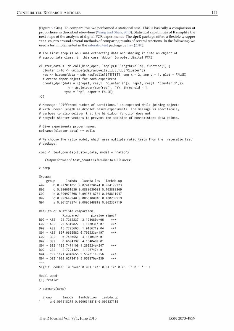
CONTRIBUTED RESEARCH ARTICLES 144
(Figure 9 G04). To compare this we performed a statistical test. This is basically a comparison ofproportions as described elsewhere (Wang and Shan, 2013). Statistical capabilities of R simplify thenext steps of the analysis of digital PCR experiments. The dpcR package offers a flexible wrappertest_counts around several methods of comparing results of several reactions. In the following, weused a test implemented in the rateratio.test package by Fay (2010).
# The first step is as usual extracting data and shaping it into an object of# appropriate class, in this case 'ddpcr' (droplet digital PCR)
cluster_data <- do.call(bind_dpcr, lapply(1L:length(wells), function(i) {cluster.info <- unique(pds_raw[wells[i]][[1]]["Cluster"])res <- bioamp(data = pds_raw[wells[i]][[1]], amp_x = 2, amp_y = 1, plot = FALSE)# create ddpcr object for each experimentcreate_dpcr(data = c(rep(1, res[1, "Cluster.2"]), rep(1, res[1, "Cluster.3"])),
n = as.integer(sum(res[1, ])), threshold = 1,type = "np", adpcr = FALSE)
}))
# Message: 'Different number of partitions.' is expected while joining objects# with uneven length as droplet-based experiments. The message is specifically# verbose to also deliver that the bind_dpcr function does not# recycle shorter vectors to prevent the addition of non-existent data points.
# Give experiments proper names.colnames(cluster_data) <- wells
# We choose the ratio model, which uses multiple ratio tests from the 'rateratio.test'# package.
comp <- test_counts(cluster_data, model = "ratio")
Output format of test_counts is familiar to all R users:
> comp
Groups:group lambda lambda.low lambda.up
A02 b 0.077011051 0.0704320674 0.084179123B02 c 0.096061636 0.0888030003 0.103883369C02 c 0.099979708 0.0918318731 0.108811947D02 c 0.092649940 0.0856180946 0.100230919G04 a 0.001218274 0.0006348818 0.002337119
Results of multiple comparison:X_squared p_value signif
B02 - A02 22.7202237 3.123089e-06 ***C02 - A02 29.5319827 1.100031e-07 ***D02 - A02 15.7795663 1.016671e-04 ***G04 - A02 897.9635582 6.799223e-197 ***C02 - B02 0.7480551 4.164049e-01D02 - B02 0.6604392 4.164049e-01G04 - B02 1132.7471108 1.260524e-247 ***D02 - C02 2.7724424 1.198747e-01G04 - C02 1171.4948655 9.557011e-256 ***G04 - D02 1092.0273410 5.950879e-239 ***---Signif. codes: 0 ‘***’ 0.001 ‘**’ 0.01 ‘*’ 0.05 ‘.’ 0.1 ‘ ’ 1
Model used:[1] "ratio"
> summary(comp)
group lambda lambda.low lambda.up1 a 0.001218274 0.0006348818 0.002337119
The R Journal Vol. 7/1, June 2015 ISSN 2073-4859

CONTRIBUTED RESEARCH ARTICLES 145
0.00
0.02
0.04
0.06
0.08
0.10
Experiment
λ
●
a
●
b
●
●
●
c c c
A02 B02 C02 D02 G04
Figure 10: Comparison of droplet digital PCR runs. The plot method of the test_counts functionfrom the dpcR package was used. The experiments were aggregated into colour coded groups basedon their estimated mean number of copies per partition (λ). A02 remained individual b, B02, C02 andD02 formed a group c and the negative control also remained individual a.
2 b 0.077011051 0.0704320674 0.0841791233 c 0.096230428 0.0887509893 0.104308745
The result of the analysis suggests that replicate samples B02, C02 and D02, with exception ofA02, do not differ significantly. The negative control G04 was totally different from the other samples(Figure 10). Our dpcR package can be used to analyse data beyond a level as provided by commercialsoftware. Access to the whole R environment allows performing more elaborated research in a highlycustomized workflow. In conclusion, our case study shows, that the R environment can be used tocircumvent problems of locked-in systems.
Discussion and conclusion
This study gave a brief introduction to the analysis of qPCR, qIA, MCA and dPCR experiments withR. In addition to this, we briefly referenced to a vast collection of additional packages available fromCRAN and Bioconductor. The packages may be considered as the building blocks (libraries) to createwhat users want and need. We showed that automatized research with R offers powerful meansfor statistical analysis and visualization. This software is not tied to a vendor or application (e.g.,chamber or droplet based digital PCR, capillary or plate qPCR). It should be quite easy even for aninexperienced user to define a workflow and to set up a cross-platform environment for specific needsin a broad range of technical settings (Figure 11). This environment enforces no monolithic integration.We claim that the modular structure allows the user to perform flexible data analysis, adjusted to theirneeds and to design frameworks for high-throughput analysis. Furthermore, R enables the users toaccess and reuse code for the creation of reports in various formats (e.g., HTML, PDF).
Despite the fact that R is free of charge, it is quite possible to build commercial applications. Thepackages cover implementation of novel approaches and peer-reviewed analysis methods. R packagesare an open environment to adopt to the growing knowledge in life sciences and medical sciences.Therefore, we argue that this environment may provide a structure for standardized nomenclature andserve as reference in qPCR and dPCR analysis. Speaking about openness, it needs to be emphasizedthat the main advantage of this software is its transparency at any time for anybody. Thus, it ispossible to track numerical errors. A disadvantage of R is the lack of comprehensive GUIs for qPCRanalysis. GUIs are key technologies to spread the use of R in bioanalytical sciences. Currently, we areestablishing the ‘pcRuniveRsum’ (http://michbur.github.io/pcRuniveRsum/) as an on-line resourcefor the interested users. The command-line structure makes R ’inaccessible’ for many novices. We try
The R Journal Vol. 7/1, June 2015 ISSN 2073-4859

CONTRIBUTED RESEARCH ARTICLES 146
Figure 11: Deployment of R applications for the qPCR and dPCR experiments. (A) R is typicallyrun from a desktop computer and operated by a GUI/IDE application such as RStudio or RKWard.This approach provides a flexible workflow for individuals. (B) Another approach is to run R withspecific applications on a local server. Such scenarios are useful for the deployment within researchdepartments or cooperate units (Nolan and Temple, 2014). (C) Cloud computing (CC) providesshared and scalable computing capacity (e.g., computing capacity, application software) and storagecapacity (e.g., databases) as a service to an individual user or a community. Service categories include:Infrastructure-as-a-Service (IaaS), Platform-as-a-Service (PaaS) and Software-as-a-Service (SaaS) over anetwork. Providers of CC manage the infrastructure and resources to achieve coherence and economiesof scale similar to a utility over a network (i.p., Internet) (Ohri, 2014).
to solve this problem with easily accessible GUIs (Rödiger et al., 2012). However, the work on thisadditions has been recently started and is still in progress.
Acknowledgment
Part of this work was funded by the BMBF InnoProfile-Transfer-Projekt 03 IPT 611X, the EuropeanRegional Development Fund (ERDF/EFRE) on behalf of the European Union, the Sächsische Auf-baubank (Free State of Saxony, Germany) and the Russian Ministry of Education and Science (projectNo. RFMEFI62114X0003), with usage of scientific equipment of Center for collective use ’Biotechnol-ogy’ at All-Russia Research Institute of Agricultural Biotechnology. We would like to thank the Rcommunity. We would like to thank Mario Menschikowski (Technical University Dresden) for thedroplet digital PCR samples.
Bibliography
M. G. Almiron, B. Lopes, A. L. C. Oliveira, A. C. Medeiros, and A. C. Frery. On the numerical accuracyof spreadsheets. Journal of Statistical Software, 34(4):1–29, 4 2010. URL http://www.jstatsoft.org/v34/i04. [p128]
R. Bååth. The state of naming conventions in R. The R Journal, 4(2):74–75, Dec. 2012. URL http://journal.r-project.org/archive/2012-2/RJournal_2012-2_Baaaath.pdf. [p129]
P. Biecek and M. Kosinski. archivist: Tools for Storing, Restoring and Searching for R Objects, 2015. URLhttp://CRAN.R-project.org/package=archivist. R package version 1.3. [p130]
K. A. Blagodatskikh, S. Roediger, and M. Burdukiewicz. RDML: Importing Real-Time Thermo Cycler(qPCR) Data from RDML Format Files, 2015. URL http://CRAN.R-project.org/package=RDML. Rpackage version 0.8-4. [p128]
L. D. Brown, T. T. Cai, and A. Dasgupta. Interval estimation for a binomial proportion. StatisticalScience, 16:101–133, 2001. [p140]
M. Burdukiewicz, S. Roediger, and B. Jacobs. dpcR: Digital PCR Analysis, 2015. URL http://CRAN.R-project.org/package=dpcR. R package version 0.1.4.0. [p127]
P. Burns. Spreadsheet addiction. online, 2014. URL http://web.archive.org/web/20141009042532/http://www.burns-stat.com/documents/tutorials/spreadsheet-addiction/. [p128]
S. A. Bustin. The reproducibility of biomedical research: Sleepers awake! Biomolecular Detection andQuantification, 2:35–42, Dec. 2014. [p127]
I. Castro-Conde and J. de Uña-Álvarez. sgof: An R package for multiple testing problems. The RJournal, 6(2):96–113, Dec. 2014. [p127]
The R Journal Vol. 7/1, June 2015 ISSN 2073-4859

CONTRIBUTED RESEARCH ARTICLES 147
W. Chang, J. Cheng, J. J. Allaire, Y. Xie, and J. McPherson. shiny: Web Application Framework for R, 2015.URL http://CRAN.R-project.org/package=shiny. R package version 0.12.1. [p31, 140]
P. Corbisier, L. Pinheiro, S. Mazoua, A.-M. Kortekaas, P. Y. J. Chung, T. Gerganova, G. Roebben,H. Emons, and K. Emslie. DNA copy number concentration measured by digital and droplet digitalquantitative PCR using certified reference materials. Analytical and Bioanalytical Chemistry, 407(7):1831–1840, 2015. [p140, 141, 143]
A. J. Durán, M. Pérez, and J. L. Varona. The misfortunes of a trio of mathematicians using computeralgebra systems. Can we trust in them? Notices of the American Mathematical Society, 2014. [p128]
H. Dvinge and P. Bertone. HTqPCR: High-throughput analysis and visualization of quantitativereal-time PCR data in R. Bioinformatics, 25(24):3325–3326, Dec. 2009. [p128]
C. Ekstrom, I. M. Skovgaard, and T. Martinussen. kulife: Datasets and Functions from the (Now Non-Existing) Faculty of Life Sciences, University of Copenhagen, 2013. URL http://CRAN.R-project.org/package=kulife. R package version 0.1-14. [p128]
M. P. Fay. Two-sided exact tests and matching confidence intervals for discrete data. The R Journal, 2(1):53–58, June 2010. [p144]
C. Gandrud. Reproducible Research with R and RStudio. Chapman and Hall/CRC, July 2013. [p129]
R. C. Gentleman, V. J. Carey, D. M. Bates, B. Bolstad, M. Dettling, S. Dudoit, B. Ellis, L. Gautier, Y. Ge,J. Gentry, K. Hornik, T. Hothorn, W. Huber, S. Iacus, R. Irizarry, F. Leisch, C. Li, M. Maechler, A. J.Rossini, G. Sawitzki, C. Smith, G. Smyth, L. Tierney, J. Y. H. Yang, and J. Zhang. Bioconductor: Opensoftware development for computational biology and bioinformatics. Genome Biology, 5(10):R80,2004. [p128, 129]
M. Guescini, D. Sisti, M. B. L. Rocchi, L. Stocchi, and V. Stocchi. A new real-time PCR method to over-come significant quantitative inaccuracy due to slight amplification inhibition. BMC Bioinformatics,9(326), July 2008. [p130]
H. Hofmann, A. Unwin, and D. Cook. Let graphics tell the story – Datasets in R. The R Journal, 5(1):117–130, June 2013. [p129]
J. Huggett, J. O’Grady, and S. Bustin. How to make mathematics biology’s next and better microscope.Biomolecular Detection and Quantification, 1(1):A1–A3, 2014. [p127]
J. F. Huggett, C. A. Foy, V. Benes, K. Emslie, J. A. Garson, R. Haynes, J. Hellemans, M. Kubista, R. D.Mueller, T. Nolan, M. W. Pfaffl, G. L. Shipley, J. Vandesompele, C. T. Wittwer, and S. A. Bustin.The digital MIQE guidelines: Minimum information for publication of quantitative digital PCRexperiments. Clinical Chemistry, 59(6):892–902, June 2013. [p127, 140]
J. F. Huggett, S. Cowen, and C. A. Foy. Considerations for digital PCR as an accurate moleculardiagnostic tool. Clinical Chemistry, 61(1):79–88, Oct. 2015a. [p140]
J. F. Huggett, J. O’Grady, and S. Bustin. qPCR, dPCR, NGS — A journey. Biomolecular Detection andQuantification, 3:A1–A5, Mar. 2015b. [p127]
M. Jahn, J. Seifert, M. von Bergen, A. Schmid, B. Bühler, and S. Müller. Subpopulation-proteomics inprokaryotic populations. Current Opinion in Biotechnology, 24(1):79–87, Feb. 2013. [p141]
M. Jahn, C. Vorpahl, D. Türkowsky, M. Lindmeyer, B. Bühler, H. Harms, and S. Müller. Accuratedetermination of pasmid copy number of flow-sorted cells using droplet digital PCR. AnalyticalChemistry, 86(12):5969–5976, June 2014. [p141]
D. A. Khodakov and A. V. Ellis. Recent developments in nucleic acid identification using solid-phaseenzymatic assays. Microchimica Acta, 181(13–14):1633–1646, 2014. [p127]
J. D. Kloke and J. W. McKean. Rfit: Rank-based estimation for linear models. The R Journal, 4(2):57–64,Dec. 2012. [p139]
M. Kohl. SLqPCR: Functions for Analysis of Real-Time Quantitative PCR Data at SIRS-Lab GmbH. SIRS-LabGmbH, Jena, 2007. URL www.sirs-lab.com. [p128]
M. Kuhn. CRAN task view: Reproducible research, 2015. URL http://CRAN.R-project.org/view=ReproducibleResearch. Version 2015-06-18. [p129]
The R Journal Vol. 7/1, June 2015 ISSN 2073-4859

CONTRIBUTED RESEARCH ARTICLES 148
T. J. Leeper. Archiving reproducible research and dataverse with R. The R Journal, 6(1):151–158, 2014.[p129]
S. Lefever, J. Hellemans, F. Pattyn, D. R. Przybylski, C. Taylor, R. Geurts, A. Untergasser, J. Vandesom-pele, and RDML Consortium. RDML: Structured language and reporting guidelines for real-timequantitative PCR data. Nucleic Acids Research, 37(7):2065–2069, Apr. 2009. [p128, 135]
Z. Liu and S. Pounds. An R package that automatically collects and archives details for reproduciblecomputing. BMC Bioinformatics, 15(1):138, May 2014. [p129]
T. Luo, L. Jiang, W. Sun, G. Fu, J. Mei, and Q. Gao. Multiplex real-time PCR melting curve assay todetect drug-resistant mutations of mycobacterium tuberculosis. Journal of Clinical Microbiology, 49(9):3132–3138, Sept. 2011. [p133]
N. Majumdar, T. Wessel, and J. Marks. Digital PCR modeling for maximal sensitivity, dynamic rangeand measurement precision. PLoS ONE, 10(3):e0118833, Mar. 2015. [p140]
J. Mar. qpcrNorm: Data-Driven Normalization Strategies for High-Throughput qPCR Data, 2009. URLhttp://bioconductor.org. R package version 1.26.0. [p128]
M. V. Matz. MCMC.qpcr: Bayesian Analysis of qRT-PCR Data, 2015. URL http://CRAN.R-project.org/package=MCMC.qpcr. R package version 1.2. [p128]
M. N. McCall1, H. R. McMurray, H. Land, and A. Almudevar. On non-detects in qPCR data. Bioinfor-matics, 30(16):2310–2316, Aug. 2014. [p128]
B. D. McCullough and D. A. Heiser. On the accuracy of statistical procedures in Microsoft Excel 2007.Computational Statistics & Data Analysis, 52(10):4570–4578, June 2008. [p128]
P. Michna. RNetCDF: Interface to NetCDF Datasets, 2015. URL http://CRAN.R-project.org/package=RNetCDF. R package version 1.7-3; with contributions from Milton Woods. [p129]
P. Michna and M. Woods. RNetCDF – A package for reading and writing NetCDF datasets. The RJournal, 5(2):29–37, Dec. 2013. [p129]
C. A. Milbury, Q. Zhong, J. Lin, M. Williams, J. Olson, D. R. Link, and B. Hutchison. Determining lowerlimits of detection of digital PCR assays for cancer-related gene mutations. Biomolecular Detectionand Quantification, 1(1):8–22, Sept. 2014. [p127, 140]
A. A. Morley. Digital PCR: A brief history. Biomolecular Detection and Quantification, 1(1):1–2, Sept. 2014.[p127]
P. Murrell. It’s not what you draw, it’s what you don’t draw. The R Journal, 4(2):13–18, Dec. 2012. [p128,129]
P. Murrell. The gridGraphics package. The R Journal, 7(1):152–163, June 2015. [p128]
J. D. Neve and J. Meys. unifiedWMWqPCR: Unified Wilcoxon-Mann-Whitney Test for qPCR Data, 2014.URL http://bioconductor.org. R package version 1.4.0. [p128]
J. D. Neve, J. Meys, J.-P. Ottoy, L. Clement, and O. Thas. unifiedWMWqPCR: The unified Wilcoxon-Mann-Whitney test for analyzing RT-qPCR data in R. Bioinformatics, 30(17):2494–2495, 2014. [p128]
G. J. Nixon, H. F. Svenstrup, C. E. Donald, C. Carder, J. M. Stephenson, S. Morris-Jones, J. F. Huggett,and C. A. Foy. A novel approach for evaluating the performance of real time quantitative loop-mediated isothermal amplification-based methods. Biomolecular Detection and Quantification, 2:4–10,Dec. 2014. [p127]
D. Nolan and D. L. Temple. XML and Web Technologies for Data Sciences with R. Springer-Verlag, NewYork, 2014. [p146]
J. Oh. Automatic conversion of tables to LongForm dataframes. The R Journal, 6(2):16–26, 2014. [p129]
A. Ohri. R for Cloud Computing – An Approach for Data Scientists. Springer-Verlag, New York, 2014.[p146]
J. Ooms. Directions for improved dependency versioning in R. The R Journal, 5(1):197–207, June 2013.[p129]
S. Pabinger, S. Rödiger, A. Kriegner, K. Vierlinger, and A. Weinhäusel. A survey of tools for the analysisof quantitative PCR (qPCR) data. Biomolecular Detection and Quantification, 1, 2014. [p127, 128, 140]
The R Journal Vol. 7/1, June 2015 ISSN 2073-4859
CONTRIBUTED RESEARCH ARTICLES 149
Y. Pan, X. Yan, and J. Li. qPCR.CT: qPCR Data Analysis and Plot Package, 2012. URL http://CRAN.R-project.org/package=qPCR.CT. R package version 1.1. [p128]
S. L. Pape. EasyqpcR: EasyqpcR for Easy Analysis of Real-Time PCR Data at IRTOMIT-INSERM U1082.IRTOMIT-INSERM U1082, 2012. URL http://irtomit.labo.univ-poitiers.fr/. [p128]
J. R. Perkins, J. M. Dawes, C. Orengo, S. B. McMahon, D. L. Bennett, and M. Kohl. ReadqPCRand NormqPCR: R packages for the reading, quality checking and normalisation of RT-qPCRquantification cycle (Cq) data. BMC Genomics, 13(296), 2012. [p128]
R Core Team. R Data Import/Export. R Foundation for Statistical Computing, Vienna, Austria, 2015.URL http://www.R-project.org/. [p129]
C. Ritz and A.-N. Spiess. qpcR: an R package for sigmoidal model selection in quantitative real-timepolymerase chain reaction analysis. Bioinformatics, 24(13):1549–1551, July 2008. PMID: 18482995.[p130]
S. Rödiger, T. Friedrichsmeier, P. Kapat, and M. Michalke. RKWard: A comprehensive graphicaluser interface and integrated development environment for statistical analysis with R. Journal ofStatistical Software, 49(9):1–34, 2012. URL http://www.jstatsoft.org/v49/i09. [p129, 146]
S. Rödiger, A. Böhm, and I. Schimke. Surface melting curve analysis with R. The R Journal, 5(2):37–53,Dec. 2013a. [p128, 130, 133, 136, 138]
S. Rödiger, P. Schierack, A. Böhm, J. Nitschke, I. Berger, U. Frömmel, C. Schmidt, M. Ruhland,I. Schimke, D. Roggenbuck, W. Lehmann, and C. Schröder. A highly versatile microscope imag-ing technology platform for the multiplex real-time detection of biomolecules and autoimmuneantibodies. Advances in Biochemical Engineering/Biotechnology, 133:35–74, 2013b. [p127, 128, 138]
S. Rödiger, C. Liebsch, C. Schmidt, W. Lehmann, U. Resch-Genger, U. Schedler, and P. Schierack.Nucleic acid detection based on the use of microbeads: A review. Microchimica Acta, 181(11–12):1151–1168, 2014. [p127, 138]
S. Rödiger, M. Burdukiewicz, and P. Schierack. chipPCR: an R package to pre-process raw data ofamplification curves. Bioinformatics, in press. doi: 10.1093/bioinformatics/btv205. [p130, 131, 139]
S. Roediger. MBmca: Nucleic Acid Melting Curve Analysis on Microbead Surfaces with R, 2015. URLhttp://CRAN.R-project.org/package=MBmca. R package version 0.0.3-5. [p128]
S. Roediger and M. Burdukiewicz. chipPCR: Toolkit of Helper Functions to Pre-Process Amplification Data,2014. URL http://CRAN.R-project.org/package=chipPCR. R package version 0.0.8-4. [p128]
RStudio Team. RStudio: Integrated Development Environment for R. RStudio, Inc., Boston, MA, 2012.URL http://www.rstudio.com/. [p129, 160]
J. M. Ruijter, M. W. Pfaffl, S. Zhao, A. N. Spiess, G. Boggy, J. Blom, R. G. Rutledge, D. Sisti, A. Lievens,K. De Preter, S. Derveaux, J. Hellemans, and J. Vandesompele. Evaluation of qPCR curve analysismethods for reliable biomarker discovery: bias, resolution, precision, and implications. Methods, 59(1):32–46, Jan. 2013. [p127, 128, 130, 133]
J. M. Ruijter, P. Lorenz, J. M. Tuomi, M. Hecker, and M. J. B. v. d. Hoff. Fluorescent-increase kinetics ofdifferent fluorescent reporters used for qPCR depend on monitoring chemistry, targeted sequence,type of DNA input and PCR efficiency. Microchimica Acta, 181(13–14):1689–1696, Oct. 2014. [p127]
D. A. Selck, M. A. Karymov, B. Sun, and R. F. Ismagilov. Increased robustness of single-moleculecounting with microfluidics, digital isothermal amplification, and a mobile phone versus real-timekinetic measurements. Analytical Chemistry, 85(22):11129–11136, Nov. 2013. [p127]
A.-N. Spiess. qpcR: Modelling and Analysis of Real-Time PCR Data, 2014. URL http://CRAN.R-project.org/package=qpcR. R package version 1.4-0. [p128]
A.-N. Spiess, C. Deutschmann, M. Burdukiewicz, R. Himmelreich, K. Klat, P. Schierack, and S. Rödiger.Impact of smoothing on parameter estimation in quantitative DNA amplification. Clinical Chemistry,61(2):379–388, 2015. [p128, 138]
D. Svec, A. Tichopad, V. Novosadova, M. W. Pfaffl, and M. Kubista. How good is a PCR efficiencyestimate: Recommendations for precise and robust qPCR efficiency assessments. BiomolecularDetection and Quantification, 3:9–16, Mar. 2015. [p130]
The R Journal Vol. 7/1, June 2015 ISSN 2073-4859
CONTRIBUTED RESEARCH ARTICLES 150
D. A. Swan. DivMelt: HRM Diversity Assay Analysis Tool, 2013. URL http://CRAN.R-project.org/package=DivMelt. R package version 1.0.3; with contributions from Craig A Magaret and MatthewM Cousins. [p128]
P. M. Valero-Mora and R. Ledesma. Graphical user interfaces for R. Journal of Statistical Software, 49(1):1–8, June 2012. URL http://www.jstatsoft.org/v49/i01. [p129]
M. van der Loo. settings: Software Option Settings Manager for R, 2015. URL http://CRAN.R-project.org/package=settings. R package version 0.2.2. [p130]
E. Viturro, C. Altenhofer, B. Zölch, A. Burgmaier, I. Riedmaier, and M. W. Pfaffl. Microfluidic high-throughput reverse-transcription quantitative PCR analysis of liver gene expression in lactatinganimals. Microchimica Acta, 181(13-14):1725–1732, Oct. 2014. [p127]
W. Wang and G. Shan. ExactCIdiff: An R package for computing exact confidence intervals for thedifference of two proportions. The R Journal, 5(2):62–71, Dec. 2013. [p144]
J. Wu, R. Kodzius, W. Cao, and W. Wen. Extraction, amplification and detection of DNA in microfluidicchip-based assays. Microchimica Acta, 181(13-14):1611–1631, Oct. 2014. [p127]
M. Zeller, W.-C. L. A. Guazzelli, and G. Williams. PMML: An open standard for sharing models. The RJournal, 1(1):60–65, June 2009. [p129]
J. D. Zhang, R. Biczok, and M. Ruschhaupt. ddCt: The ddCt Algorithm for the Analysis of QuantitativeReal-Time PCR (qRT-PCR), 2015. URL http://bioconductor.org. R package version 1.22.0. [p128]
Stefan Rödiger (corresponding author)Faculty of Natural SciencesBrandenburg University of Technology Cottbus–[email protected]
Michał BurdukiewiczUniversity of WroclawFaculty of BiotechnoloyDepartment of [email protected]
Konstantin BlagodatskikhAll-Russia Research Institute of Agricultural BiotechnologyCenter for collective use ’Biotechnology’[email protected]
Michael JahnHelmholtz Centre for Environmental Research - UFZFlow cytometry group / Environmental [email protected]
Peter SchierackFaculty of Natural SciencesBrandenburg University of Technology Cottbus–[email protected]
The R Journal Vol. 7/1, June 2015 ISSN 2073-4859