1. Introduction to R 2. About Hue Tom Wheeler Cloudera, Inc.

St. Louis Hadoop User Group December 16, 2014

What is R?

!   Language for statistical computing

!   Re-implementation of the S programming language

!   Open source (GNU license)

!   A pirate's favorite language?

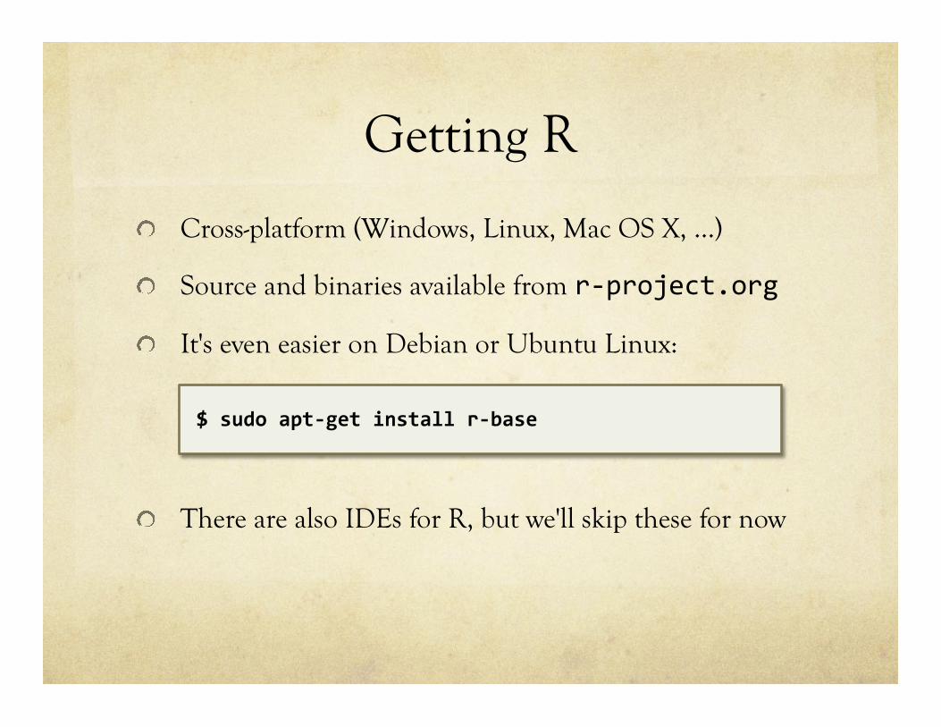
Getting R

!   Cross-platform (Windows, Linux, Mac OS X, …)

!   Source and binaries available from r-­‐project.org  

!   It's even easier on Debian or Ubuntu Linux:

!   There are also IDEs for R, but we'll skip these for now

$  sudo  apt-­‐get  install  r-­‐base  

Starting R in Interactive Mode

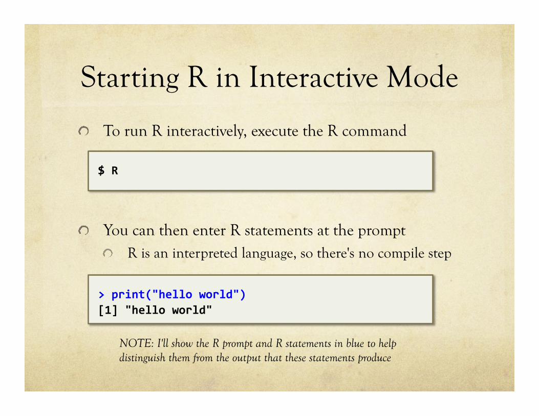
!   To run R interactively, execute the R command

!   You can then enter R statements at the prompt !   R is an interpreted language, so there's no compile step

$  R  

>  print("hello  world")  [1]  "hello  world"    

NOTE: I'll show the R prompt and R statements in blue to help distinguish them from the output that these statements produce

Exiting Interactive Mode

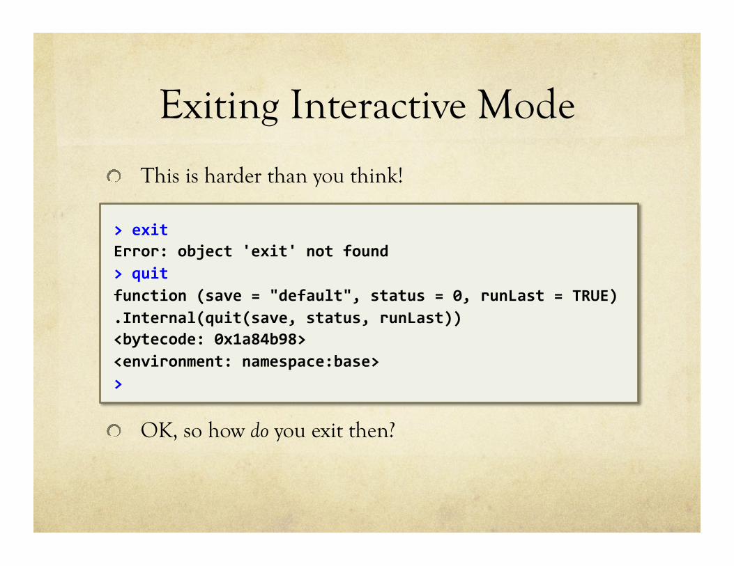
!   This is harder than you think!

!   OK, so how do you exit then?

>  exit  Error:  object  'exit'  not  found  >  quit  function  (save  =  "default",  status  =  0,  runLast  =  TRUE)    .Internal(quit(save,  status,  runLast))  <bytecode:  0x1a84b98>  <environment:  namespace:base>  >    

Exiting Interactive Mode, Part II

!   Use the quit() function, or its short equivalent, q()  !   Alternatively, you can hit Ctrl-d

!   You can avoid this prompt by starting R thusly

$  R  -­‐-­‐no-­‐save  

>  quit()  Error:  object  'exit'  not  found  >  Save  workspace  image?  [y/n/c]:  n  $  

Running R Scripts

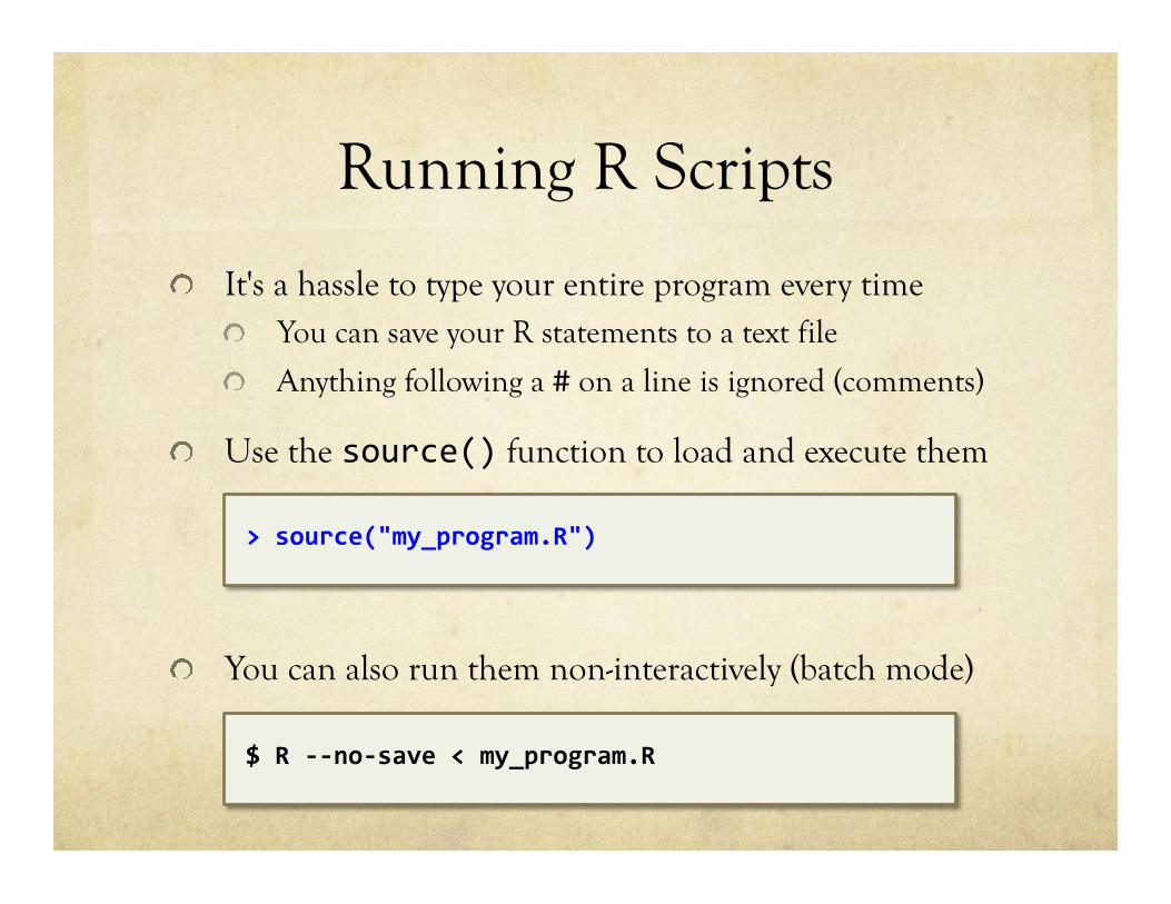
!   It's a hassle to type your entire program every time !   You can save your R statements to a text file

!   Anything following a # on a line is ignored (comments)

!   Use the source() function to load and execute them

!   You can also run them non-interactively (batch mode)

$  R  -­‐-­‐no-­‐save  <  my_program.R  

>  source("my_program.R")  

R Packages and CRAN

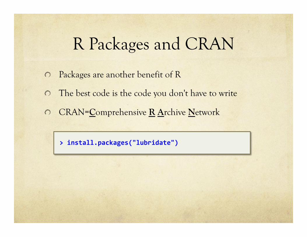
!   Packages are another benefit of R

!   The best code is the code you don't have to write

!   CRAN=Comprehensive R Archive Network

>  install.packages("lubridate")    

Assignment and Types

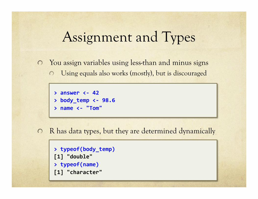
!   You assign variables using less-than and minus signs !   Using equals also works (mostly), but is discouraged

!   R has data types, but they are determined dynamically

>  answer  <-­‐  42  >  body_temp  <-­‐  98.6  >  name  <-­‐  "Tom"  

>  typeof(body_temp)  [1]  "double"  >  typeof(name)  [1]  "character"  

Why the [1] in the Output?

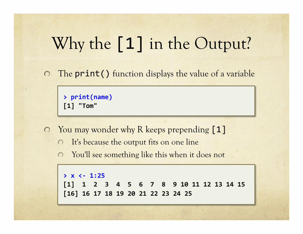
!   The print() function displays the value of a variable

!   You may wonder why R keeps prepending [1]  !   It's because the output fits on one line

!   You'll see something like this when it does not

>  print(name)  [1]  "Tom"  

>  x  <-­‐  1:25  [1]    1    2    3    4    5    6    7    8    9  10  11  12  13  14  15    [16]  16  17  18  19  20  21  22  23  24  25  

Vectors

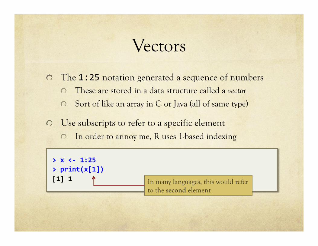
!   The 1:25 notation generated a sequence of numbers !   These are stored in a data structure called a vector

!   Sort of like an array in C or Java (all of same type)

!   Use subscripts to refer to a specific element !   In order to annoy me, R uses 1-based indexing

>  x  <-­‐  1:25  >  print(x[1])  [1]  1   In many languages, this would refer

to the second element

Vectors Abound!

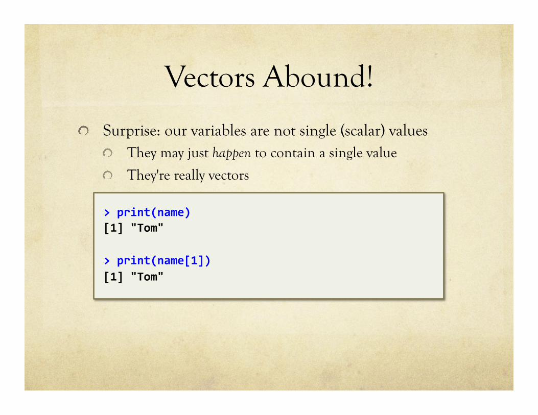
!   Surprise: our variables are not single (scalar) values !   They may just happen to contain a single value

!   They're really vectors

>  print(name)  [1]  "Tom"    >  print(name[1])  [1]  "Tom"  

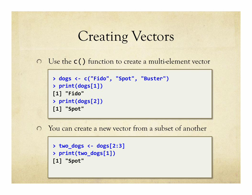
Creating Vectors

!   Use the c() function to create a multi-element vector

!   You can create a new vector from a subset of another

>  dogs  <-­‐  c("Fido",  "Spot",  "Buster")  >  print(dogs[1])  [1]  "Fido"  >  print(dogs[2])  [1]  "Spot"  

>  two_dogs  <-­‐  dogs[2:3]  >  print(two_dogs[1])  [1]  "Spot"  

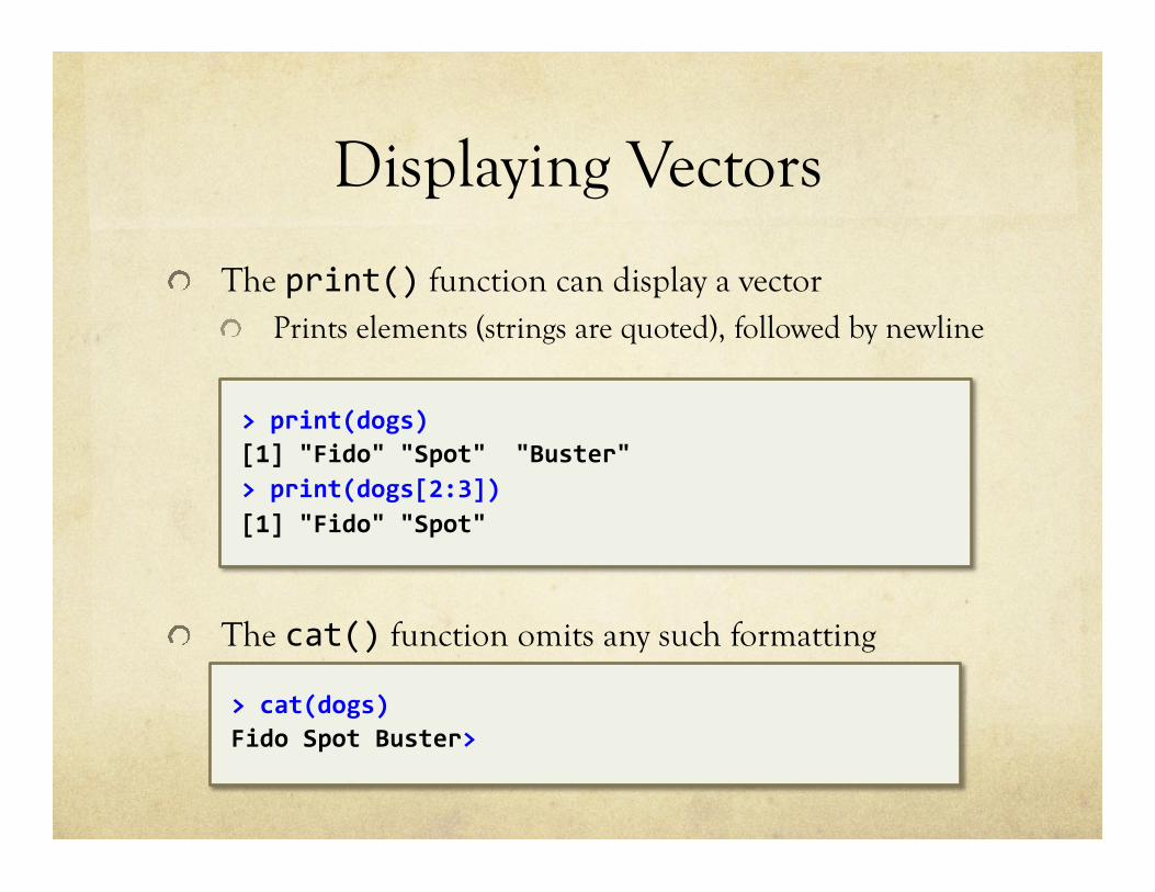
Displaying Vectors

!   The print() function can display a vector !   Prints elements (strings are quoted), followed by newline

!   The cat() function omits any such formatting

>  print(dogs)  [1]  "Fido"  "Spot"    "Buster"  >  print(dogs[2:3])  [1]  "Fido"  "Spot"  

>  cat(dogs)  Fido  Spot  Buster>  

Generating Random Numbers

!   You saw earlier how to generate a sequence of numbers !   R can also generate random numbers

!   The rnorm() function generates N random numbers !   Based on the normal distribution (AKA "bell curve")

!   Values are centered about zero

>  z  <-­‐  rnorm(8)  >  print  (z)  [1]  -­‐0.6935897  -­‐2.1828442    1.7268656    0.1267711    [5]  -­‐0.3590410  -­‐0.8488329  -­‐1.7032515  -­‐0.6952838  

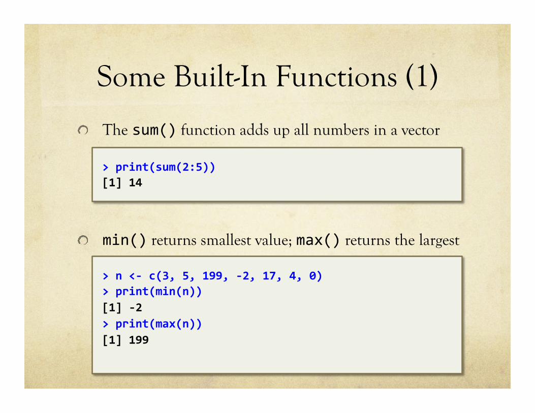
Some Built-In Functions (1)

!   The sum() function adds up all numbers in a vector

!   min() returns smallest value; max() returns the largest

>  print(sum(2:5))  [1]  14  

>  n  <-­‐  c(3,  5,  199,  -­‐2,  17,  4,  0)  >  print(min(n))  [1]  -­‐2  >  print(max(n))  [1]  199  

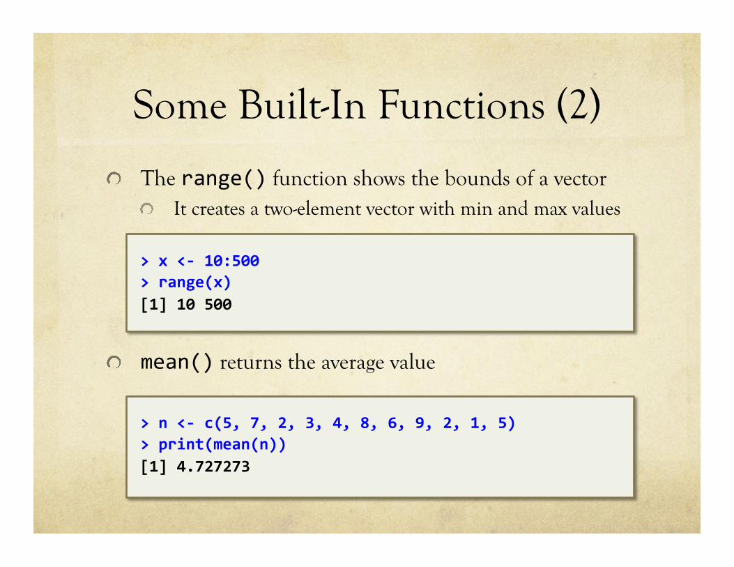
Some Built-In Functions (2)

!   The range() function shows the bounds of a vector !   It creates a two-element vector with min and max values

 

!   mean() returns the average value

>  x  <-­‐  10:500  >  range(x)  [1]  10  500  

>  n  <-­‐  c(5,  7,  2,  3,  4,  8,  6,  9,  2,  1,  5)  >  print(mean(n))  [1]  4.727273  

Some Built-In Functions (3)

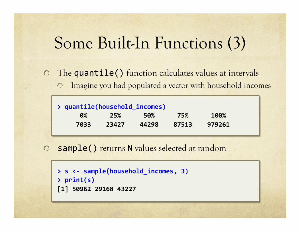
!   The quantile() function calculates values at intervals !   Imagine you had populated a vector with household incomes

 

 

!   sample() returns N values selected at random

>  quantile(household_incomes)              0%            25%            50%            75%            100%            7033        23427        44298        87513        979261  

>  s  <-­‐  sample(household_incomes,  3)  >  print(s)  [1]  50962  29168  43227  

Creating Functions

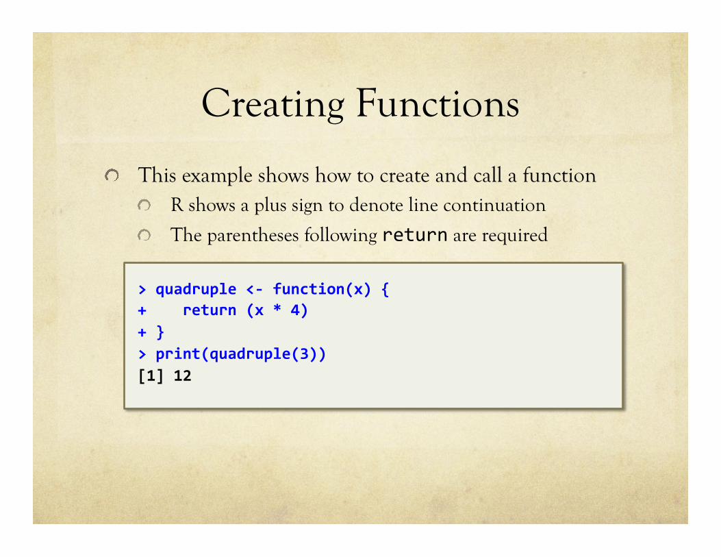
!   This example shows how to create and call a function !   R shows a plus sign to denote line continuation

!   The parentheses following return are required

>  quadruple  <-­‐  function(x)  {  +        return  (x  *  4)  +  }  >  print(quadruple(3))  [1]  12  

Applying Functions to Vectors

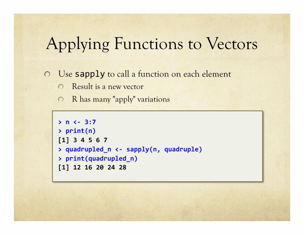
!   Use sapply to call a function on each element !   Result is a new vector

!   R has many "apply" variations

>  n  <-­‐  3:7  >  print(n)  [1]  3  4  5  6  7  >  quadrupled_n  <-­‐  sapply(n,  quadruple)  >  print(quadrupled_n)  [1]  12  16  20  24  28  

Lists

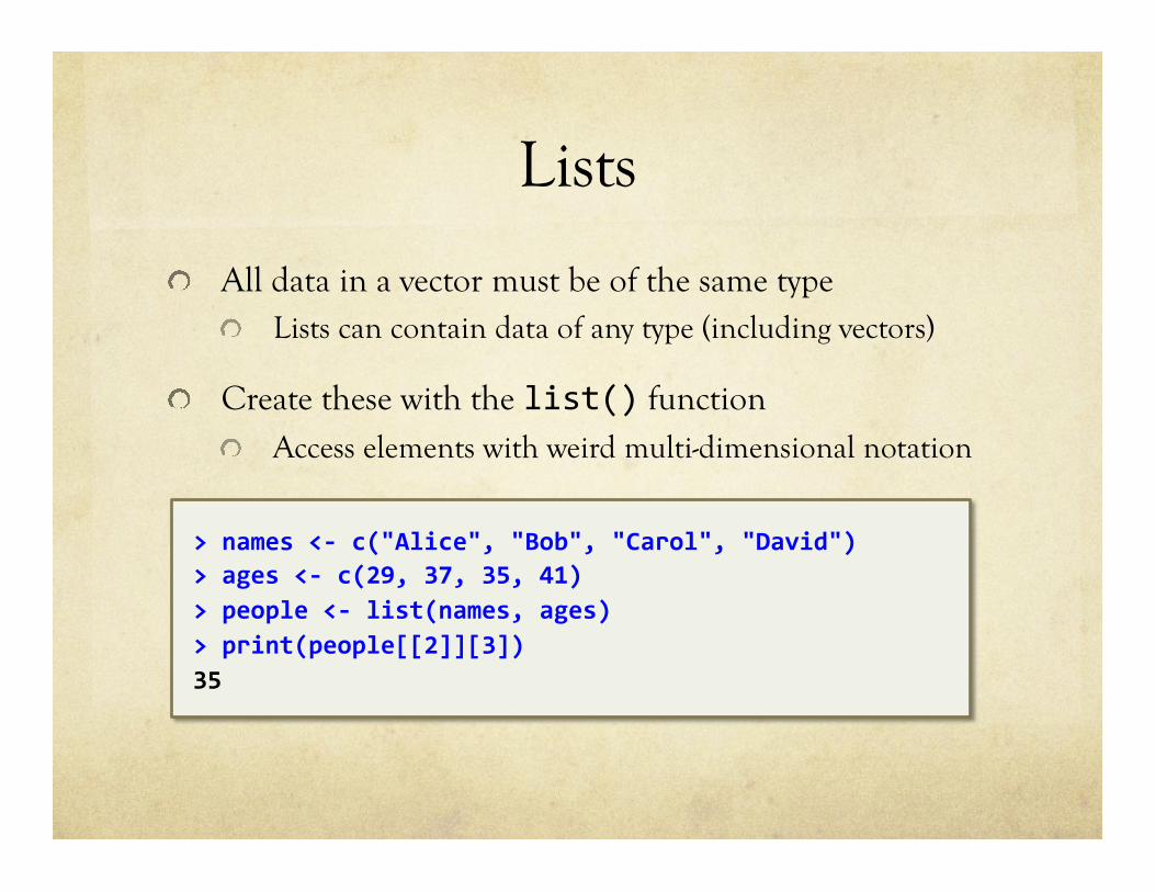
!   All data in a vector must be of the same type !   Lists can contain data of any type (including vectors)

!   Create these with the list() function !   Access elements with weird multi-dimensional notation

>  names  <-­‐  c("Alice",  "Bob",  "Carol",  "David")  >  ages  <-­‐  c(29,  37,  35,  41)  >  people  <-­‐  list(names,  ages)    >  print(people[[2]][3])    35  

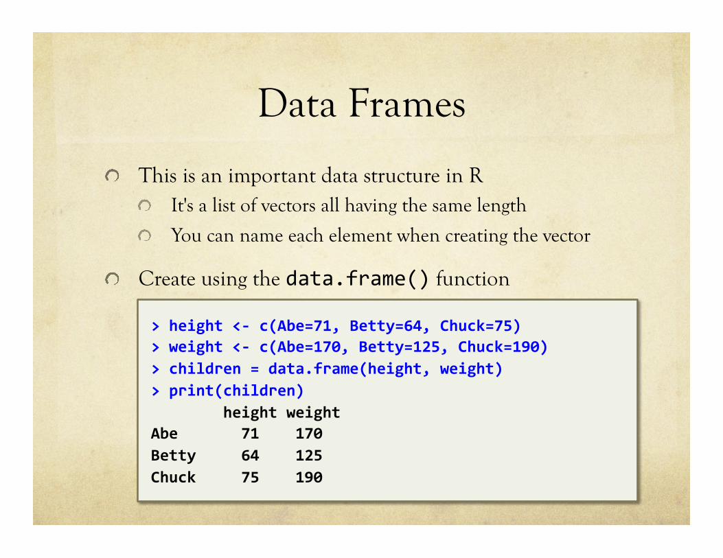
Data Frames

!   This is an important data structure in R !   It's a list of vectors all having the same length

!   You can name each element when creating the vector

!   Create using the data.frame() function

>  height  <-­‐  c(Abe=71,  Betty=64,  Chuck=75)  >  weight  <-­‐  c(Abe=170,  Betty=125,  Chuck=190)  >  children  =  data.frame(height,  weight)  >  print(children)                  height  weight  Abe              71        170  Betty          64        125  Chuck          75        190  

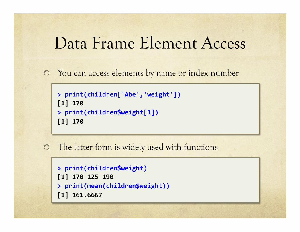
Data Frame Element Access

!   You can access elements by name or index number

!   The latter form is widely used with functions

>  print(children['Abe','weight'])  [1]  170  >  print(children$weight[1])  [1]  170  

>  print(children$weight)  [1]  170  125  190  >  print(mean(children$weight))  [1]  161.6667  

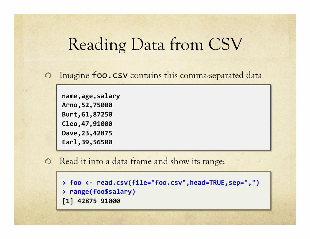
Reading Data from CSV

!   Imagine foo.csv contains this comma-separated data

!   Read it into a data frame and show its range:

>  foo  <-­‐  read.csv(file="foo.csv",head=TRUE,sep=",")  >  range(foo$salary)  [1]  42875  91000  

name,age,salary  Arno,52,75000  Burt,61,87250  Cleo,47,91000  Dave,23,42875  Earl,39,56500  

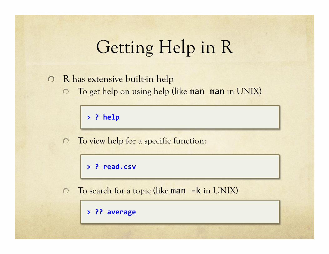
Getting Help in R

!   R has extensive built-in help !   To get help on using help (like man  man in UNIX)

!   To view help for a specific function:

!   To search for a topic (like man  -­‐k in UNIX)

>  ?  help  

>  ?  read.csv  

>  ??  average  

Graphics

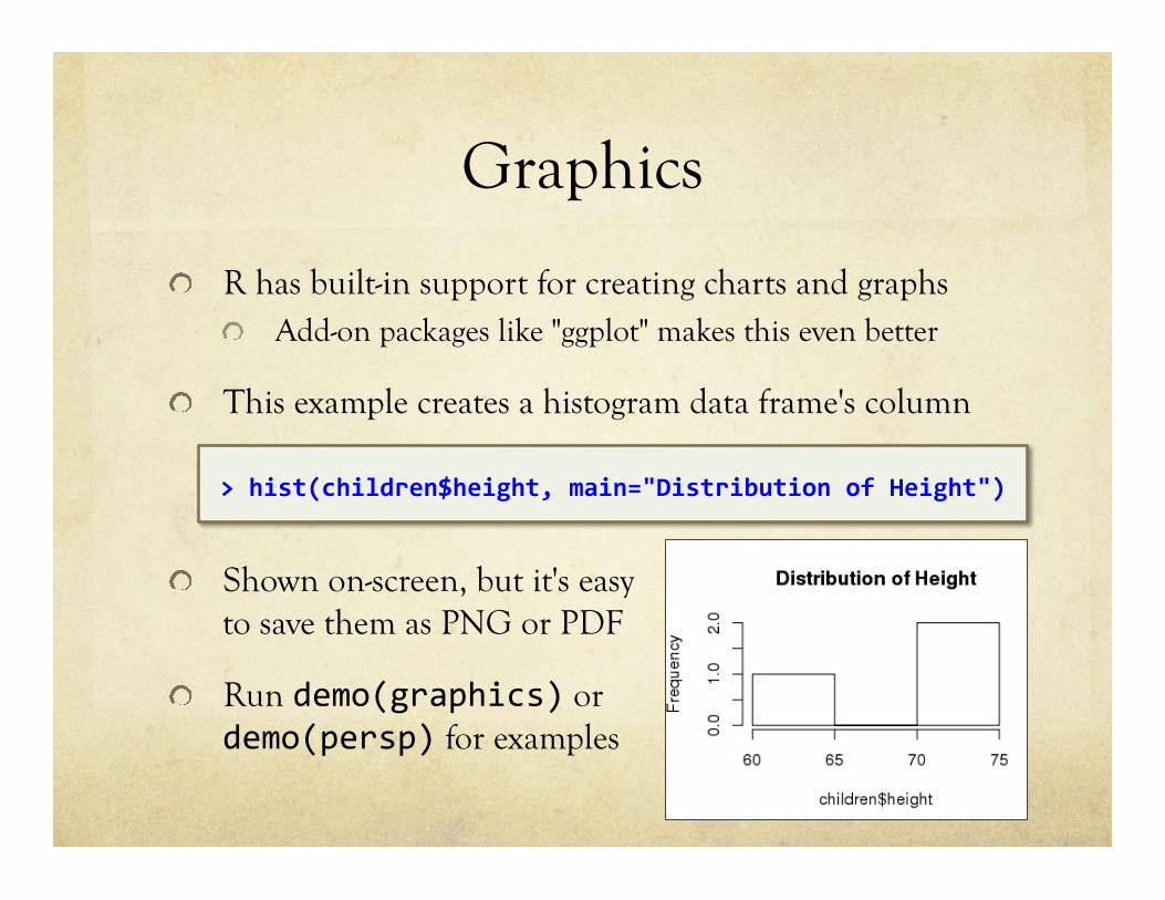
!   R has built-in support for creating charts and graphs !   Add-on packages like "ggplot" makes this even better

!   This example creates a histogram data frame's column

!   Shown on-screen, but it's easy

to save them as PNG or PDF

!   Run demo(graphics) or demo(persp) for examples

>  hist(children$height,  main="Distribution  of  Height")  

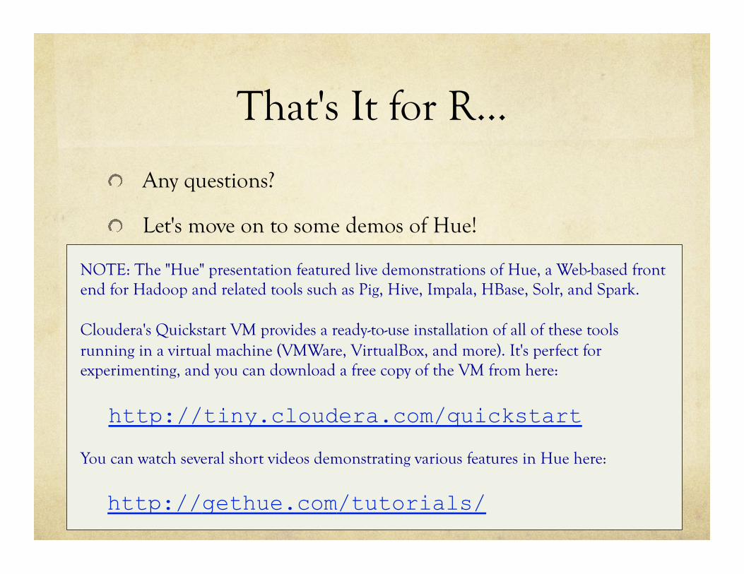
That's It for R…

!   Any questions?

!   Let's move on to some demos of Hue!

NOTE: The "Hue" presentation featured live demonstrations of Hue, a Web-based front end for Hadoop and related tools such as Pig, Hive, Impala, HBase, Solr, and Spark. Cloudera's Quickstart VM provides a ready-to-use installation of all of these tools running in a virtual machine (VMWare, VirtualBox, and more). It's perfect for experimenting, and you can download a free copy of the VM from here:

http://tiny.cloudera.com/quickstart You can watch several short videos demonstrating various features in Hue here:

http://gethue.com/tutorials/