NUWC-NPT Technical Report 10,4051 October 1993

CN

mE A Predictive Parametric Model for Volume'• Scattering Strength in the Deep Ocean With an

Application to Nighttime Near-Surface Scatteringn R in the North Sargasso Sea Below 16 kHz

R. Alfred SaengerWendy L WachterEnvironmental and Tactical Support Systems Department

DTICS ELECTEAPR0 7 199411

E4A% 94- 10486

Naval Undersea Warfare Center DetachmentNew London, Connecticut

Approved for public release; distribution Is unlimited.

94 4 6 013

4*

PREFACE

This document was prepared under Project No. D20027, "Multi-StaticSonar Program (MSS)," Principal Investigator R. Christian (Code 3112) andProgram Manager C Mason (Code 304). The Sponsoring Activity is the ProgramExecutive Office-Undersea Warfare (PEO-USW), Project Manager Darrell Spires(Advanced Systems and Technology Office-Cl) under Program Element 63553N.

The technical reviewer for this report was R. Christian (Code 3112).

Reviewed and Approved: 1 October 1993

B. F. ColeHead, Environmental and Tactical Support

Systems Department

REPORT DOCUMENTATION PAGE 06.f,, "180~bamgmuuW110111 IIIub Or hMr ba .Is d~-N 6 ann I how W WaPeM. ua~

gdw~ k*a•1 We1fo moduft O b w .bmmI W&ftWi4m sweiS. bo 1215Mk0w f ,,, t .,,..120.A ,, VA 2 ,204 ,,,lo 0. CA.• ,,,,u, , , . ,, USNS

1. AGENCY USE ONLY (Leave OWN 2. REPORTE 3. REPORT TYPEAND DATESCOVEREDI October 1993 Final

4. TITLE AND SUBTITLE 5. FNNG NUMBERSA Predictive Parametric Model for Volume Scattering Strength in the DeepOcean with an Application to Nighttime Near-Surface Scattering in the PE 602936North Sargasso Sea Below 16 kHz

6. AU

R. Alfred Saenger and Wendy L. Wachter

7. PERFORMING ORGANIZATION NAME(S) AND ADDRESS(ES) 8. PERFORMING ORGANIZATIONREPORTNUMBER

Naval Undersea Warfare Center Detachment39 Smith Street TR 10,405New London, Connecticut 06320-5594

9. SPONSORING/MONITORING AGENCY NAME(S) AND ADDRESS(ES) 10. SPONSORING/MONITORINGAGENCY REPORT NUMBER

Naval Sea Systems Command2531 Jefferson David HighwayArlington, VA 22242-5160

11. SUPPLEMENTARY NOTES

12a. DISTRIBUTIONIAVAILABILITY STATEMENT 12b. DISTRIBUTION CODE

Approved for public release; distribution is unlimited.

13. ABSTRACT (Ma~dmum 200 words)

In the deep ocean, long range active sonars are often volume reverberation limited at night due to scatteringfrom the gas-filled swimbladders of mesopelagic fish In near-surface waters. To predict the detection performanceof these sonars with a general sonar model, volume scattering strength profiles Sv(z,f) are needed as inputs. Ageneral volume scattering strength model (VSSM) for nighttime/daytime Sv(z,f) profiles in a deep water faunalprovince is described. Explicit expressions are developed for the average length-depth distribution of bladderedfish, the corresponding swimbladder radius-depth distribution, and volume scattering strength Sv(z,f). A specificnighttime near-surface VSSM is developed for the North Sargasso Sea faunal province using data from Ocean Acreexperiment 12. A VSSM of very simple form is found capable of describing measured nighttime profiles at 3.85and 15.5 kHz to a depth of 225 m. This agreement, however, could only be obtained by modifying modelparameters obtained from trawl data to correct for sampling deficiencies, principally net avoidance by the larger fish.Predictions with the modified VSSM at 1 kHz suggest that in the nighttime 0-50 m surface layer, Sv-levels were ashigh as -75 dB due to scattering from these larger fish.

14. SUBJECT TERMS 15. NUMBER OF PAGESVolume scattering strength model Ocean Acre scattering layers Swimbladder target strength 46Bioacoustic volume scattering model Mesopelagic bladdered fish scatterers Swimbladder 0-factor 16. PRICE CODE

17. SECURITY CLASSIFICATION 18. SECURITY CLASSIFICATION 19. SECURITY CLASSIFICATION 20. UMITATION OF ABSTRACTOF REPORT OF THIS PAGE OF ABSTRACT

Unclassified Unclassified Unclassified SARNSN 7540-01-280-6500 S6drFo 29S (Rev 2-N)

Pms~ by ANSI Sid Z30-18298-102

Table of Contents

PageLIST OF ILLUSTRATIONS ii

I. INTRODUCTION

II. A PARAMETRIC PHYSICAL MODEL FOR PREDICTING VOLUME 3

SCATTERING STRENGTH IN THE DEEP OCEAN (VSSM)

2.1 Biological Modeling Methodology 42.2 Bioacoustic Modeling Methodology 10

III. A SUMMER NIGHTTIME VSSM FOR NEAR-SURFACE WATERS OF 13

THE NORTH SARGASSO SEA APPLICABLE FOR LOW SONAR

SEARCH FREQUENCIES

3.1 Biological Conditions at Ocean Acre and the 16Selection of a VSSM

3.2 Predictions with the Single Scattering Layer 21

Component VSSM

IV. CONCLUSIONS AND RECOMMENDATIONS 34

V. REFERENCES 36

APPENDIX A: Theoretical Representation for the Al

Characteristic Fish Length-DepthDensity Distribution of a Scattering

Layer Component in the VSSMAPPENDIX B: Summary of the Simplified Andreeva Bi

Swimbladder Target Strength Model

i

LIST OF ILLUSTRATIONS

Figure Page

1. Representative theoretical Q(z)min, Q(z)ean , and

Q(z)aax curves based on a simplified form of

Andreeva's (1964, 1972) model that includes onlyradiation and viscous damping losses. Respective

values of #-#r +i aim used to generate these curves

are shown in the header. Experimental data fromTable 1 are included. . . . . . . . . . . . . . . . . 15

2. Resonance frequency vs depth domains for scatterers

in the nominal life stage size classes of the

Ocean Acre 18 predominant bladdered speciesgroup . . . . . . . . . . . . . . . . . . . . . . . . 19

3. TBSN predictions of nighttime S v(z,f)Qmin (lowercurve) and SV(Z,f)Qmax (upper curve) compared withOA12N experimental profiles of Fisch and Dullea(1973) taken approximately 24 hours apart: Fig.(3a), f-3.85 kHz; Fig. (3b), f-15.5 kHz ......... ... 24

4. TBSM predictions of nighttime S V(z,f)Qmin andSv(z,f)Qmax for f-0.5 kHz (Fig. 3a) and f-1.0 kHz(Fig. 3b) . . . . . . . . . . . . . . . . . . . . . . 26

5. Number density distribution n(z) for the TBSM;Modified TBSM. The characteristic density

distribution n(z) is the same in each model butthe respective standing crops are different:

N-0.72/m2 and N-4.93/m.... ...... .............. ... 29

6. (a) Fish length pdfs p(L); p(L) for the TBSM;Modified TBSM. (b) Corresponding swimbladderradius pdfs q(R); q(R) for the two models ........ ... 30

7. Modified TBSM predictions S V(z,f)Qmin (lower curve)and Sv (z,f)Qmax (upper curve) compared with OA12N

ii

Figure Page

nighttime experimental profiles of Fisch andDullea (1973) taken approximately 24 hours apart:

Fig. (7a), f-3.85 kHz; Fig. (7b), f-15.5 kHz . . . . . 31

8. Predictions with the Modified TBSM of nighttime

Sv (z,fIQmin (lower curve) and Sv (z,f)Qaax (upper

curve) for f-0.5 kHz (Fig. 8a) and f-1.0 kHz(Fig. 8b) . . . . . . . . . . . . . . . . . . . . . . 33

LIST OF TABLES

Table Page

1. Swimbladder resonance frequency and Q measured forvarious live swimbladdered fish with swimbladders

believed to be intact ......................... 14

2. Parameters and statistical properties of the

lognormal pdfs used in the Trawl-Based Sv (z,f)

Model (TBSM) and the Modified TBSM . . . ......... 23

Accesion For

NTIS CRA&IDTIC TABUnannounced UJustification .........

By .... ..... .................. .....................

Distribution I,,, a bip ,,tAvailability Codes

Avail awd I orDist Special

SA

i

A PREDICTIVE PARAMETRIC MODEL FOR VOLUME SCATTERING STRENGTH INTHE DEEP OCEAN WITH AN APPLICATION TO NIGHTTIME NEAR-SURFACE

SCATTERING IN THE NORTH SARGASSO SEA BELOW 16 kHz

I. INTRODUCTION

In the deep ocean, volume reverberation below 20 kHZ is

caused principally by resonant and nonresonant scattering from

the gas-filled swimbladders of numerous species of mesopelagic

fish most of which are diel vertical migrators. At night, a

significant fraction of these bladdered fish scatterers rise from

daytime depths to feed on zooplankton in a 200 m subsurface

layer. Under commonly occurring propagation conditions, these

near-surface scattering layers can significantly lower the

detection performance of long range 2-5 kHz search sonars. To

predict the nighttime detection performance of such sonars for

shallow targets, volume scattering strength profiles Sv (z,f) for

these layers must be provided as inputs to sonar performance

prediction models. The objective is to show how Sv-profiles can

be parametrically modeled in the deep ocean and, by way of

illustration, develop a nighttime summer model for the North

Sargasso Sea.

A predictive theoretical model for S(z,f) requires submodels

for the length-depth distribution of the scatterers, the

swimbladder sizes they contain, and the scattering properties of

the swimbladders. First we present a general theoretical model

for predicting Sv (z,f) in a deep water faunal province (Backus

and Craddock 1977). This model is then specifically tailored to

describe nighttime near-surface volume scattering in the North

Sargasso Sea during summer. Bioacoustic data from OA12, one of

the most successful of the Ocean Acre experiments (Brown and

Brooks, 1974), are used to formulate the model. We note here

that the Ocean Acre measurement site is a 1-degree quadrangle

southeast of Bermuda centered at 320N, 640W and that it is a

"typical" location in the North Sargasso Sea faunal province

(Brooks 1972, Backus and Craddock 1977).

The motivation for our parametric modeling approach stems in

part from the limitations of discrete-depth biological sampling.

In the Ocean Acre experiments (Brown and Brooks 1974, Gibbs et

al. 1987), discrete-depth biological samples were obtained with a

3-m Isaacs Kidd Midwater Trawl (IKMT) and concurrent measurements

of S(z,f) for frequencies between 3.85 and 15.5 kHz were obtained

with narrow-beam transducers (Fisch and Dullea 1973 and Fisch

1977). While the seasonal biological properties of bladdered

fish at the Ocean Acre site have been qualitatively established

by these trawl measurements, the data are inadequate for

bioacoustic prediction, as found by Brown and Brooks (1974) and

Brooks and Brown (1977). This is due to the sampling

deficiencies of the IKMT caused by net avoidance and escapement,

further complicated by patchiness and practical limitations on

the volume of water that can be sampled at each depth.

As will be demonstrated, a "Trawl Based S(z,f) Model" (TBSM)

with parameters obtained directly from OA12N data leads to

unsatisfactory agreement between predicted and measured values of

2

Sv (z,f) at 3.85 kHz, as might be expected for the reasons given

above. Because of the parametric nature of the VSSM, however,

those parameters defining the theoretical length-depth

distribution of the scatterers can be adjusted to compensate for

sampling deficiencies. The "Modified TBSMO thus obtained will be

shown to produce dramatically better agreement between predicted

and measured Sv-profiles at 3.85 kHz and 15.5 kHz. Sv-predictions

are also made at the nominal frequencies 0.5 and 1.0 kfz at which

scattering from mesopelagic fish is commonly assumed to be

negligible. The large differences between corresponding

predictions with the two models at 3.85, 15.5, 0.5, and 1.0 kHz

are physically explained with the help of a resonance

frequency/depth diagram for the various life stage size classes

of the bladdered fish population.

II. A PARAMETRIC PHYSICAL MODEL FOR PREDICTING VOLUME SCATTERING

STRENGTH IN THE DEEP OCEAN (VSSM)

In section 2.1 we first formulate an idealized theoretical

model for the length-depth distribution n(L,z) of swimbladdered

fish. The approach was suggested by the seasonal depth

distribution patterns of bladdered fish observed in the Ocean

Acre experiments which are believed to be fairly typical of many

deep ocean areas. For bioacoustic modeling, the swimbladder

radius-depth distribution n(R,z) is required, and the procedure

for transforming n(L,z) to n(R,z) is considered next. Then, in

section 2.2, a general theoretical formulation for the volume

backscatter coefficient sv (z,f) is given. It contains a

simplified form of Andreeva's (1964, 1972) model for swimbladder

3

target strength in which contributions of heat loss to aamping at

resonance are ignored. The height of the swimbladder target

strength resonance peak is determined by Q(z), the inverse

damping factor at resonance. Representative minimum, mean, and

maximum values of Q(z) in general accord with experimental values

are proposed for S-predictions with the VSSM. These are obtained

from the simplified form of Andreeva's formula for Q(z), using

suitable choices for the complex shear modulus of fish tissue.

2.1 Biological Modeling Methodology

Definitions of fish length-depth density distributions

and associated variables. Consider the swimbladder fish

population in some deep ocean faunal province during either

nighttime (N) or daytime (D) periods when the distribution of the

scatterers is approximately steady state due to the absence of

substantial vertical migration. For simplicity, N/D distribution

conditions are assumed to be spatially and temporally homogeneous

over horizontal x,y planes for all depths of interest. We define

the fish length-depth density distribution n(L,z) such that

n(L,z)dLdz represents the average number of scatterers with

lengths L...L+dL at depths z...z+dz below lm 2 of sea surface

anywhere within the faunal province. It is convenient to refer

this distribution to the average number of scatterers N below lm2

of sea surface, the "standing crop," and write

(1) n(L,z) - NA(L,z)

Awhere n(L,z) is the fish length-depth density distribution per

unit standing crop. We assume that annual variations in seasonal

4

distribution properties are solely due to annual vatiations in

the seasonal standing crop N. This permits us to interpret

A(Lz) as a "characteristics seasonally invariant measure of the

N/D distribution properties of the faunal province.

The quantity 9(Ls) may also be interpreted as a two

dimensional probability density distribution function. From

probability theory, we can write it as

(2) A(L,z) - A~zpLlz),

Awhere n(z) is a probability density function (pdf) in the depth

variable z and p(Ljz) is the conditional L-pdf for depth z. The

marginal L-pdf associated with A(L,z) is

a

(3) p(L) - J A(L,z)dz P

0

while its marginal z-pdf is

(4) A(z) - J A(L,z)dL

0

The average number density n(z), i.e., the average number of fish

per unit volume at depth z, is given by

(5) n(z) - NA(z)

Formulation for n(L,z) in the VSSM. Over a given depth

range of interest, n(L,z) is expressed as a sum of density

distributions ni(L,z) corresponding to i-1,2, .... different

5

"scattering layer components*,

(6) n(L,z) - j ni(L,z)

A scattering layer component may represent an individual

bladdered fish species or a group of such species treated as a

single "equivalent" bladdered species. Distribution properties

of mesopelagic fish are size-dependent, which complicates

biological modeling. Depending on the frequencies and depth

range for which Sv is to be predicted, not all size classes of

fish may be significant contributors to scattering. Restricting

the size range of bladdered fish in scattering layer components

to just those sizes of specific acoustic interest may simplify

the modeling of ni(Lz) in some instances. Seasonal biological

properties of the bladdered fish fauna, time-of-day, and the

depths and frequency ranges for which Sv(z,f) is to be predicted

must all be considered in chosing the appropriate scattering

layer components for any particular VSSM.

The distribution properties of the ith scattering layer

component are formally analogous to those of n(L,z) described

above. Letting Ni be the standing crop and ni(L,z)-ni(z)pi(Llz)

the characteristic distribution of the i th scattering layer

component, we may write n(L,z) as

(7) n(L,z) -A NA(z)pi(Llz)1

The particular characteristic distributions ni(L,z) employed

in the prototype VSSM are briefly described as follows (see

6

Appendix A for details). Consider a positive valued variate e>0

which is lognormally distributed. The lognormal pdf of 0,

designated here by X(G;eu, 2 ), is given by

(8) 0(; /,u2 a 2 ~ ii] EXP [-(202 r-1 (lne-#)2]

where p and v2 are the parameters of the distribution. As shown

in Appendix A, the characteristic distribution

Ai(Lz)-ni(z)pi(LIz) for an ith scattering layer component is

defined by five statistical parameters, [pi,taUxi,Oxi,pi]. In

terms of these parameters,

(9) Wi(z) - 2(z;)i,e•)

(10) pi(Llz) - L;# 2

-k(L;xi÷ I• C"i I

- XL +Pxi pi("* )[() i] , crx3 [1_P21)xi Ri

where, in the first distribution parameter of pi(Llz), Eq. (10),

M(z)-ln(z/d), with d-1 m. When pi*O, some statistical properties

of fish length such as the mean, e.g., vary systematically with z

throughout the i th layer, due to the change in form of pi(Llz)

with depth. (Equations for the z-dependence of the mode, median,

and mean of pi(Llz) are given in Appendix A.) If the random

variates L and z are statistically independent for the ith

7

scattering layer component, then pi-0, and we have a "simple ith

scattering layer component". For such components, length

distribution properties are independent of depth, as may be seen

by putting pi-O in Eq. (10). Then the conditional pdf pi(LIz)2

reduces to the marginal pdf pi(L)-X(L;pxi,uxi ), Eq. (A2), in

Appendix A. This length pdf and all statistical properties

associated with it remain the same at all depths throughout the

ith simple scattering layer component.

If the scattering layer components of n(L,z) are all simple

layers, then n(L,z) in Eq. (7) becomes

(11) n(L,z) - 1j NiAi(z)pi(L)

Nix(z;pi, oi2) X(L;uxi, Oxi

AThe characteristic distribution ni(L,z) for each ith simple layer

is specified by four parameters, [Pi,•i,oxixi] and the scale of

its contribution to n(L,z) is set by the layer standing crop

factor Ni.

Transformation of n(L,z) to n(R,z). Each bladdered

mesopelagic fish of length L is assumed to contain a fully

inflated swimbladder with an equivalent spherical radius R.

Replacing L by R in Eqs. (7) and (11) for n(L,z), we have the

corresponding formal expressions

(12) n(R,z) - NiA i(z)qi(Rjz)

and

(13) n(R,z) - 7 NiAi(z)qi(R)1

for n(R,:). To obtain explicit expressions for n(R,X) in these

equations, transformations Pi(Llz) --- qi(RJZ) and pi(L)---*qi(R)

must be performed.

Due to swimbladder size variability in mesopelagic fish, it

is desirable for purposes of transformation to use a more

realistic swimbladder size allometry model than that afforded by

ban allometric law regression curve R-aLb. Bivariate normal

models are available for Ocean Acre bladdered species and

bladdered species groups (Saenger 1989). If such models are used

as a basis for transformation, then it can be shown (Saenger

1988) that qi(RIz) is a lognormal pdf with distribution 2

parameters depending on the parameters y and ax2 of

Pi(LIz), Eq. (10), and other quantities:

(14) qi(RIz) - X(R;uyii•, 2

with

(15) Pyijc lna + bp

and

(16) 2 b 2 2

- b xi yX

where a and b refer to the allometric law curve R-aLb associated

with the bivariate model, and s 2 is a constant obtained from

the model that, simply put, expresses the spread of swimbladder

size about the regression curve. For the special case pi-0,

9

where we are dealing with a simple scattering layer, the

transformed distribution qi(R) obtained from pi(L), Eq. (A2), is

also lognormal, and is given by

(17) qi(R) - XR;# 2yi,)yl)

with

(18) Pyi - lna + bpxi

and

(19) y xi ylx

Swimbladder variability extends the frequency bandwidth of the

scattering so, if possible, it should be taken into account to

reduce prediction errors in Sv. (See Saenger 1988 for discussion

and examples).

2.2 Bioacoustic Modeling Methodology

The volume backscatter coefficient sv(Z,f). Randomly

dispersed or loosely aggregated bladdered fish are assumed so

that scattering contributions from individual swimbladders may be

summed incoherently. Following conventions introduced by Urick

(1983), the volume backscatter coefficient sv(z,f) may be

expressed as

(20) sv(z,f) - n(z)x(z,f)/d 2, m-3

where T(z,f) is the average target strength in m2 of swimbladders

10

of all size found at depth z for an ensonifying frequency f.

(Some prefer to omit d 2 -1m 2 from this definition, in which case

the resulting volume backscatter coefficient mv (z,f) has

dimensions d- 1 .) From probability theory, r(z,f) is computed

from

(21) r(zef) - Jq(Rlz)r 0 (R,z,f)dR, a2

0

where 0 (R,z,f) is the target strength in m2 of a gas-filled

swimbladder of radius R cm at depth z for frequency f. Combining

Eqs. (20) and (21) and remembering that n(z)q(RJz)-n(R,z)-NA(R,z),

sv may be written as

(22) sv(zf) - NJA(R,z)[I 0 (Rz,f)/d 2 ]dR

0

- N9v( (z,f)

A

where 5v(z,f) in m-1 is the volume backscatter coefficient per

unit standing crop. This expression points up the central

importance of the characteristic swimbladder radius-depthAdistribution n(R,z) as a biological input. It follows from our

Abiological assumptions that sv (z,.f) is an invariant

characteristic measure of seasonal volume scattering properties

in the faunal province.

The volume scattering contribution s Vi(z,f) from each ith

scattering layer component has a form similar to that for sv (z,f)

in Eq. (22), viz.,

11

(23) evi (z,f) - Ni~vi(zf)

Due to the assumption of incoherent scattering, svi-contributions

from each ith component can be added to give sv(z,f). with L andR in cm and z in a, the formal theoretical expressions for

Sv(z,f) in the VSSM are summarized as follows:

(24) Sv(z,f) - 10 log [sv(z,f)d3], dB re 1/i3

(25) sv(z,f) -)m Ni~vi(z,f),

(26) kvi (Zz) - Ai(z) fqi(RIz)[I 0 (R,z,f)/d 2 ]dR, m-1

0

(27) ni(z) - X(z;pi,i 2), m-1

(28) qi(Rlz) - X(R;uyii 2 ,,yi cm 1

For a simple ith scattering layer component, qi(RIz) in Eqs. (26)

and (28) is replaced by qi(R) given in Eq. (17). At present,

full computer implementation of these equations exists only for

simple scattering layer components. In numerically calculating

2vi(z,f), Eq. (26), for such a component, digitally sampled,Atruncated, and renormalized pdfs hli(z) and qi(R) are used, and

the integral is evaluated using the trapezoid rule.

The simplified Andreeva model for swimbladder target

strength. In the VSSM, a simplified form of Andreeva's (1964,

1972) model for swimbladder target strength T0 (R,z,f) is used in

which only radiation and viscous damping losses are retained in

the theoretical expression for Q(z), the reciprocal damping

12

constant at resonance. The equations of this model as used in

the VSSM are summarized in Appendix B.

In modeling volume scattering strength in the deep ocean, it

is not possible to measure the many variables that determine the

Q of fish swimbladders. Therefore, in the context of the

simplified Andreeva model, we propose the adoption of provisional

phenomenological values for the complex shear modulus p m r +ipA im

of fish tissue that give values of Q in reasonable agreement with

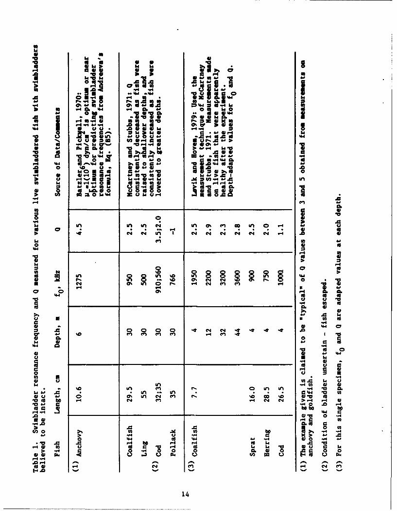
experiment. Some available experimental data are shown in Table

1. Measurements of Q(z) made near the surface are of the order

of 3 to 5. Assuming such results are applicable to mesopelagic

fish, and taking #r=l(10 6 ) dyn/cm2 as recommended by Batzler and

Pickwell (1970), Q(z) was computed from Eq. B(10) using different

values of #im" By trial-and-error, the "Representative Minimum,

Mean, and Maximum Q(z) curves shown in figure 1 were obtained.

These curves encompass many of the Q(z) values in Table 1, and

the trends of the theoretical Q(z) curves with depth are at least

consistent with the observations of McCartney and Stubbs (1971).

VSSM predictions displayed below utilize one or other of these

Q(z) curves, as noted.

III. A SUMMER NIGHTTIME VSSM FOR NEAR-SURFACE WATERS OF THE

NORTH SARGASSO SEA APPLICABLE FOR LOW SONAR SEARCH

FREQUENCIES

The VSSM provides a general formalism for modeling the

length-depth distribution n(L,z) of biological scatterers in a

faunal province. The objective here is to select the simplest

13

.rI %w4 US0 soI4

'9~~ 0 -

61 S .S05 b

.940~ be~4e

IV :b0.3at 40 to C . D.~ A IW r- %*0 IOI "q -4LeW t 4 J4iS4 " 94 "4. Clio~ I) to r-4 I

4J e. I' 6e.N 014 :0).4 .. .A) be N "440 aW u C go 0

to aC U.4a Ur

b.9

be P. in IA D 0% C ") C4 %D0 '-

U6 v4~ IA d

GowU Sa

00

*~~ c.J Ln VA 0 s 1- .C"L. T.I in4 04 V

O 0"1 0 . 0.

Ao W0 0 0 0 4 bo c. 4 4 0 0e

4.0 q9p 6

0 44 ( 944 "4 0 "

V A Ar-4 o t- r-4w' A

r-45 U)"40 b

r-4-903 9.4 C ' - . "

14

Plot of O(z) - Simplified Andreevc ModelM ,-R dynes/cm.*2 1.0000+06 1.0000+06 I.0000+06M-IMdynes/cm.*2 2.500D+06 1.5000+06 1.0000+06

o .

0e I II

0 50 100 150 200 250z, m

Figure 1. Representative theoretical Q(z)min, Q(Z)mean, and Q(z)maxcurves based on a simplified form of Andreeva's (1964, 1972)model that includes only radiation and viscous dampinglosses. Respective values of p-pr+ipim used to generatethese curves are shown in the header. Experimental data fromTable 1 are included.

15

model capable of predicting S(z,f) between the surface and a

depth of the order of 200 m for sonar frequencies up to about 15

kHz. This requires consideration of the broad features of OA12N

biological data and their physical implications. Unfortunately,

average trends in the length-depth distributions of bladdered

fish are obscured by the unknown efficiency of the IKMT net and

sampling fluctuations accentuated by the low densities of

bladdered fish and patchiness. Consequently, the choice of model

is somewhat subjective. The ultimate justification for any

particular model is that it involve as few theoretical parameters

as possible and that it is capable of predicting experimental

values of S(z,f). In the section below, a very simple model for

n(L,z) is proposed based on distribution properties inferred from

OA12N trawl data. Predictions with this model are maae in the

following section where it is shown that, due primarily to net

avoidance by the larger fish, model parameters derived from trawl

data must be modified to obtain realistic predictions.

3.1 Biological Conditions at Ocean Acre and the Selection of a

VSSM

Using trawl data from the major Ocean Acre experiments

together with swimbladder size allometry information, Brown and

Brooks (1974) identified 55 predominant swimbladdered fish taxa

at Ocean Acre. The size-depth distribution properties of these

fish during the spring (OA10,14), summer (OA12), and winter

(OA13) were studied in detail by Brooks and Saenger (1991). In

the OA12N nighttime 0-200 m layer, these fish have individual

16

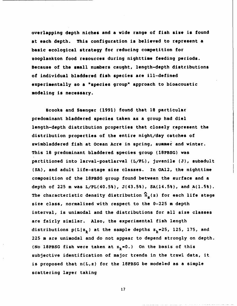
overlapping depth niches and a wide range of fish size is found

at each depth. This configuration is believed to represent a

basic ecological strategy for reducing competition for

zooplankton food resources during nighttime feeding periods.

Because of the small numbers caught, length-depth distributions

of individual bladdered fish species are ill-defined

experimentally so a *species group" approach to bioacoustic

modeling is necessary.

Brooks and Saenger (1991) found that 18 particular

predominant bladdered species taken as a group had diel

length-depth distribution properties that closely represent the

distribution properties of the entire night/day catches of

swimbladdered fish at Ocean Acre in spring, summer and winter.

This 18 predominant bladdered species group (18PBSG) was

partitioned into larval-postlarval (L/PL), juvenile (J), subadult

(SA), and adult life-stage size classes. In OA12, the nighttime

composition of the 18PBSG group found between the surface and a

depth of 225 m was L/PL(40.5%), J(43.5%), SA(14.5%), and A(l.5%).

The characteristic density distribution ns (z) for each life stage

size class, normalized with respect to the 0-225 m depth

interval, is unimodal and the distributions for all size classes

are fairly similar. Also, the experimental fish length

distributions p(LJzk) at the sample depths zk-25, 125, 175, and

225 m are unimodal and do not appear to depend strongly on depth.

(No 18PBSG fish were taken at zk-0.) On the basis of this

subjective identification of major trends in the trawl data, it

is proposed that n(L,z) for the 18PBSG be modeled as a simple

scattering layer taking

17

(29) n(L,s) - NA(z)p(L)

Further, to represent the swimbladder size allometry properties

of this group, it seems most appropriate to use an "equivalent

bivariate normal" model developed by Saenger (1989) for a

subgroup of 50 Ocean Acre nonregressive swimbladdered fish taxa

drawn from the list of 55 OA predominant swimbladdered fish taxa

given by Brown and Brooks (1974). Regression equation constants

(a,b) and s2 from this model are found at the bottom of Table 2ylx

below. The swimbladder radius-depth distribution corresponding

to n(L,z) in Eq. (29) is n(R,z)-NA(z)q(R), and the parameters

(#yo y2) of the lognormal pdf q(R) are obtained from those of

p(L) using Eqs. (18) and (19). Finally, the expression for

sv (z,f) in this VSSM is obtained by substituting Nn(z)q(R) for

NA(R,z) in Eq. (22).

Physical implications and possible limitations of this very

simple model are conveniently discussed with the help of figure

2, a resonance frequency/depth diagram for the different size

classes. The 9 cm representative upper bound for the A class is

suggested by modeling results in the next section. Nominal

L-boundary values between each size class were transformed to

corresponding R-values using R-aLb, and resonance frequencies

f 0 (R,z) were then plotted as a function of depth using Andreeva's

formula, Eq. (B5). From Eq. (29) it is seen that Nn(z)

represents the average number of bladdered fish of all sizes at

depth z. The relative proportions of the different size classes

18

Swimblodder Resonance Frequency vs z for Various Fish Lengths LL(cm) 1.3500+00 2.2500+00 3.3500+00 9.0000+00

Paraeters: a = 3.384D-02 b = 8.9190-01 MU-R = 1.0000+06 dynes/cma.2

2LARVAL- /

N /. CaS12

UADULTo ~ L-2.25 c

4-•

L-9. 0 CA

0 50 100 150 200 250

Z m

Figure 2. Resonance frequency vs depth domains for scatterers in thenominal life stage size classes of the Ocean Acre 18predominant bladdered species group.

19

are determined by p(L) and are the same at each depth in this

model. For a given sonar frequency f, contributions to Sv(z,f)

from fish of a particular size will be greatest at those depths

where the resonance frequency f 0 (R,z) of their swimbladders is

equal to, or near, f. Since x0 (R,z,f 0 ) - Q 2R2 from Eq. (B3),

such contributions from large fish at low kHz frequencies can be

very important, even when these fish are present in relatively

low numbers. Therefore the accuracy of low frequency predictions

with this VSSM depends critically on the tail portion of the

model pdf p(L).

The size pass band limitations of the IKMT and the expected

large summer increase of L/PL fish at Ocean Acre must both be

considered in assessing the probable effectiveness of the

proposed model for n(L,z). Gibbs and Karnella (1987) tentatively

estimated the range of fish size efficiently sampled by the 3-m

IKMT to be 1-5 cm. With regard to the larger fish, comparison of

OA12N non-discrete depth oblique catches with the much larger

Engel trawl suggest that adult fish are inadequately represented

in the IKMT catches. Brooks and Brown (1978) reported that while

the range of fish size obtained with both nets was similar, the

mean lengths of fish caught with the Engel trawl were commonly

twice as large. In particular (private communication), they

found the nighttime size distribution for a group of 6 species

(which incidentally happen to belong to the 18PBSG) to be

unimodal, with the mode of the IKMT distribution at 1.2 cm and

that for the Engel distribution at 2.6 cm. Thus, it is very

probable that the larger adult fish are not present in the IKMT

catch. Also, it is very probable that the L/PL size class is

20

undersampled, since the estimated decrease in catch efficiency of

the INMT occurs over much of the L/PL size range.

If the summertime L/PL size class is actually a larger

fraction of the 18PBSG than is indicated by the lINT catch, it

might be necessary to use a more general n(L,z) model than that

proposed in Eq. 29. In view of the size-dependent differences in

life style expected of the L/PL and (J+SA+A) size groups, one

might treat these size groups as independent scattering layer

components. Or, individual size classes might be treated as

independent scattering layer components in an even more refined

model. However, trawl data provide no definitive evidence for

the need of one or other of these more complex models, so we

shall explore the predictive capability of the single scattering

layer component model, the simplest of the various possible

VSSMs.

3.2 Predictions with the Single Scattering Layer Component VSSM

The Trawl-Based S Model (TBSM). Predictions in the TBSM are

made with model parameters derived solely from OA12N lINT sample

data for the 18PBSG taken at the depths zk-0, 25, 125, 175, and

225 m. No attempt has been made to correct the parameters for

sampling deficiencies. [N,p,,o 2 ,x ,ax2 were calculated as

follows. Estimates of N and the moments z and z-of the

experimental normalized density distribution referred to the

0-225 m depth interval were obtained using procedures described

in Brooks and Saenger 1991. The parameters (u,ov) n(z) were

then derived from Y and z by the method of moments (Aitchison

21

2L

and Brown 1957). The parameters (xox 2 ) of p(L) were -omputed

as density-weighted averages of [px(zk),Ox 2(zk)I. The latter

were calculated by applying the method of moments to experimentalvalues of t(zk) and L--(Zk). Then the parameters (#y,•y 2 )

2defining q(R) were obtained from (xax ) using Eqs. (18) and(19) with allometric constants a,b, and s2 from the 50

swimbladdered fish taxa bivariate normal model mentioned above.

Table 2 contains the TBSM parameters so obtained and some

statistical properties of the distributions n(z) and p(L).

TBSM predictions S(z,f)Omin and S(z,f)Qmax for 3.85 kHz are

compared with OA12N experimental Sv-profiles obtained on two

successive nights by Fisch and Dullea (1973) in Fig. (3a). The

agreement is very poor. From our previous considerations, some

of the shortfall in overall level may be supposed due to the

model value for standing crop N being too low. However, the

increasing divergence of the depth trend of predicted and

experimental values is consistent with the expectation that

important scattering contributions from larger fish are missing

from the model. As seen from figure 2, contributions from adult

fish are expected to be sizable at 3.85 kHz, not only because of

the large size of their swimbladders, but because scattering

occurs at a frequency equal to, or not too far from, the

resonance frequency of their swimbladders.

At 15.5 kHz, Fig. (3b), agreement with experiment is still

poor, but there is now less discrepancy in overall level and

depth trends of predicted and experimental values. From figure

2, this may be tentatively explained by noting that at this

22

""4 eqm .ms

"4% 3- .

14 0 -I A" O

a b.554 9* A3

.V5 "4"

A; .4 00 04 6 C ;.1 0

a .p4- 05

"in -4 " r4 P

U. IV1. 5 555-440 " Q(-

- g'fl~iSAC 40( C4 '45 ~'0

4-tKr- 44'b

* 0.04* _ _ _ _ _ _ _ _ _ _ _ _ _ _N. u

04 0 -4.44"q4 %WEVU

5~~~ ~6 =. 9 (1 14

be P4 0.00. o e 0)

9 C4

U i I) a 41H4 a-Uo 0 . 5o14C 0

10 r-c0 0V

5) "-1 v- U-

SIV C: U) Ur N )W "

% (~ 0~4 n ' a 0 '" (4 44

4I CAin4.

".0 V qv '4 OSqH~~U 0 v) 000 . r

I~ U)m = X 4 0% '

23. ~ 4 )

OA12N TRAWL-BASED S(z.f) PREDICTION MODEL. f=3.85 kHzCOMPARISON OF EXPERIMENTAL WITH MINIMUM AND MAXIMUM PREDICTED VALUES

-60-* 31 AUG 71, 2230

A 0 A A71, 130

S* , A A *

-- -80-

-110 •

0 50 100 150 200 250

D e pth Z. m

OA12N TRAWL-BASED S(z,f) PREDICTION MODEL, f=15.5 kHz

COMPARISON OF EXPERIMENTAL WITH MINIMUM AND MAXIMUM PREDICTED VALUES

* 31 AUG 71, 2148

m A ,A 01 SEP 71, 2153

-70 'aA

- 80 -

S-90 •

N

(A)

-1 10--

0 50 100 150 200 250

Depth z. m

Figure 3. TBSM predictions of nighttime S v(Z,f)Omin (lower curve) and

S v(z,f)Qmax (upper curve) compared with OA12N experimental

profiles of Fisch and Dullea (1973) taken approximately 24hours apart: Fig. (3a), f-3.85 kHz; Fig. (3b), f-15.5 kHz.

24

higher frequency, and for the depths where comparison is

possible, dominant scattering contributions very likely came from

J and SA fish that on the whole are expected to have been sampled

more efficiently.

TBSK predictions for f-0.5 and 1.0 kHz are shown in figures

(4a) and (4b), respectively. In each plot, the two curves are

practically identical, since Q does not affect the form of

Sv(z,f) at these low frequencies. Here Rayleigh-type scattering

is occurring so, in m2 T 0 (R,zf)110- 4 (f/f 0 )4 R2 , with R in cm.

This explains the systematic 12 db difference in predicted values

of Sv(z,f) at the two frequencies. The lowness of the predicted

levels is presumably caused by the absence of scattering

contributions from the larger fish that would be the dominant

contributors to Sv at these low frequencies.

A Modified TBSN with model parameters corrected for net

sampling deficiencies. The choice of TBSM parameters requiring

modification to obtain agreement of VSSN predictions with

experiment involves a number of physical considerations. First,

it seems reasonable to assume that n(z) obtained from the TBSH

provides a reasonable approximation for the actual characteristic

density distribui-ion. This assumption is prompted by the

following observations: 1) n(z) can be expressed as a sum of

contributions (Ns/N)fs (z) from each sth size class, where N is

the standing crop of the sth size class; 2) s (z)-nsn(z)/Ns, by

its definition, tends to be independent of a net sampling

efficiency factor for the snth size class; 3) s(z) for the L/PL

and J size classes are virtually identical; and 4) these two size

25

RANGE OF OA12N TRAWL-BASED S(z,f) PREDICTIONS FOR f-0.5 kHz

- 110-

-120

1-30-

U(A- 150

-160 ,,

0 50 100 150 200 250

Depth z. m

RANGE OF OA12N TRAWL-BASED S(zf) PREDICTIONS FOR f=l

-1 10-

-120-

E

-140

- 1

(B)-160-1

o 50 100 150 200 250

Depth z, m

Figure 4. TBSM predictions of nighttime S (z,f)Qmin and S v(z,f)Omax for

f-0.5 kHz (Fig. 3a) and f-1.0 kHz (Fig. 3b).

26

classes constitute 84% of the 18PBSG catch between the surface

and 225 a depth. Assuming, then, that (#,a2 ) are adequate, only

the parameters (N,#x#,x 2) need modification. In estimating these

parameters, we primarily utilize experimental Sv-data at 3.85

kHz, the lowest frequency for which experimental data from OA12N

are available, since scattering contributions from larger fish

missed by the IKHT are best represented in this data.

The average length-depth density in the Modified TBSM is

designated by

(30) A(L,z) -A(z)j(L)

2 X(z;p,q2 )(L;xx ) 2

The parameters of p(L) were obtained by systematically modifying

those of p(L) in such a way as to increase the relative

proportion of larger fish in the distribution without unduly

suppressing the smaller size class components. This was done by

successively increasing the 3 cm 97.5% fractile point of p(L) to

6 cm, 9 cm, 15 cm... The corresponding transformed pdfs j(R)

were used to predict S(z f)Qmean at 3.85 and 15.5 kHz. For each

case, the standing crop parameter N was obtained by equating

interval column strengths for the 23-221 m depth interval

computed from the predicted and experimental 3.85 kHz

S v-profiles. Selection of the "optimum" Modified TBSM was

necessarily somewhat subjective. Properties satisfied by the

model finally chosen were the following:

27

1. Physical reasonableness of the 97.5% fractile points of

the p(L) and q(R) distributions;

2. Acceptable agreement in the depth trends of 3.85 kHzASV(z,f)Qmean and experimental Sv-profiles, apart from

absolute levels;

3. N such as to give better agreement in predicted levels

at 15.5 kHz than were obtained with the TBSM.

Model constants and statistical information for the Modified TBSM

are given in Table 2.

The number density distributions n(z) in the TBSM and

Modified TBSM are shown in figure 5. It is seen that, to get the

agreement with measured Sv-values shown below, a larger standing

crop is required. Also, the relative proportion of larger fish

must be increased, as seen in figure (6a). These results imply

that both the absolute values of fish density and the size ranges

of fish caught with the IKMT are seriously biased. Corresponding

swimbladder size pdfs are compared in figure (6b).

The relative increase in large swimbladder radii in the

Modified TBSM has a substantial impact on the predicted levels of

Sv at 3.85 and 15.5 kHz, as may be seen by comparing Figs. (3a)

and (7a) and Figs. (3b) and (7b). These results indicate that

the single scattering component VSSM can provide acceptable fits

to measured Sv-profiles at frequencies where different size

classes in the bladdered fish population are the dominant

scatterers. This implies that the length-depth distribution of

bladdered fish given by the Modified TBSM is very likely fairly

28

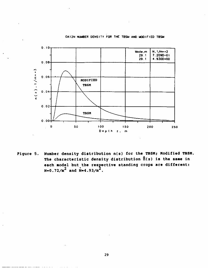
OA12N NUMBER DENSITY FOR THE TBSM AND MODIFIED TBSM

0.10.

Mode.m N.1/ms*229.1 7.209D-0i29.1 4.9300+00

0.08-

E 0.06-E MODIFIED

- TBSM

N 0.04

C

0 .02-TBSM

o.000 50 100 150 200 250

Depth z. m

Figure 5. Number density distribution n(z) for the TBSMj Modified TBSM.A(Z

The characteristic density distribution n(z) is the same in

each model but the res ective standing crops are different:

N-0.72/m2 and N-4.93/m

29

1 .0"

0.8-

E --p(L)u 0.6-

J 0.4

p(L)

0.2 '-

(A)0.0 , 1 , ,

0 3 6 9 12 15

Fish Length L. cm

106 I. q(R)

1 6-

E12

8 4(R) __ _ _ _ _ _ _ _

4- (B )

0I

0.0 0.1 0.2 0.3 0.4 0.5

Swimb ladder Radius R, cm

Figure 6. (a) Fish length pdfs p(L); p(L) for the TBSM; Modified TBSM.

(b) Corresponding swimbladder radius pdfs q(R); q(R) for the

two models.

30

OA12N MODIFIED TRAWL-BASED S(z.f) PREDICTION MODEL. (=3.85 kHz

COMPARISON OF EXPERIMENTAL WITH MINIMUM AND MAXIMUM PREDICTED VALUES

-50-~* 31 AUG 71, 2230

- a 01 SEP 11# 2130

-60-

0

- 70 A

_8 -

-90-

(A)- I I II

0 50 100 150 200 250

Depth z. m

OA12N MODIFIED TRAWL-BASED S(z.f) PREDICTION MODELf=15.5 kHzCOMPARISON OF EXPERIMENTAL WITH MINIMUM AND MAXIMUM PREDICTED VALUES

-50-* 31 AUG 71, 2148

- 01 SEP 71, 2153

-60-

0-9

4(B

a)

0 10-

0 50 100 150 200 250

Depth z. m

Figure 7. Modified TBSM predictions SV(z,f)Qmin (lower curve) and

Sv(z,f)Qmax (upper curve) compared with OA12N nighttime

experimental profiles of Fisch and Dullea (1973) taken

approximately 24 hours apart: Fig. (7a), f-3.85 kHz;

Fig. (7b), f-15.5 kHz.

31

realistic, and that substantially more fish, particularly larger

ones, are present than is indicated by discrete depth

measurements with the IKMT.

Finally, predictions of Sv(z,f) at 0.5 and 1.0 kHz are shown

in figures (8a) and (8b). Comparison with the corresponding TBSM

predictions in figures (4a) and (4b) shows a marked increase in

predicted levels at both frequencies and also changes in profile

shape, particularly in the 1.0 kHz profile, due to the inclusion

of scattering contributions from larger fish. Since the

resonance frequencies f 0 of the swimbladders of these larger fish

are not very far above 0.5 and 1.0 kHz at shallow depths,

differences in Q now have a perceptible effect on predicted

values at these depths, as seen in figures (Ba) and (Sb).

32

MODIFIED TRAWL-BASED S(z.f) MODEL PREDICTIONS USING MINMAX O(z) f-0.5 kHz

-80-

-90-

-100-

-110_

I

-120-

-130 ,,

0 50 100 150 200 250

Depth z. m

MODIFIED TRAWL-BASED S(zf) MODEL PREDICTIONS USING MIN.MAX O(z):f=1.0 kHz

-60-

-70 ,

S-80

-90

-110 1

0 50 100 150 200 250

Depth z, m

Figure 8. Predictions with the Modified TBSM of nighttime Sv (z,f)Qmin

(lower curve) and Sv(z,f)Qmax (upper curve) for f-0.5 kHz

(Fig. 8a) and f-1.0 kHz (Fig. 8b).

33

IV. Conclusions & Recommendations

In deep water, long range active sonars can be volume

reverberation limited at night due to scattering from small

mesopelagic swimbladdered fish present in near-surface waters.

The effect of these scatterers on detection performance in a

given propagation situation can be predicted with a general sonar

model if a scattering strength profile Sv(z,f) is available.

A parametric volume scattering strength model (VSSM) for

predicting nighttime/daytime volume scattering strength profiles

Sv(z,f) in a deep water faunal province for frequencies-below 20

kHz has been presented. The volume backscatter coefficient

S v(z,f) is formulated as the product of a normalized volume

backscatter coefficient representing the characteristic

scattering properties of the province for a particular season,

and the seasonal standing crop of bladdered fish scatterers which

generally varies from year-to-year. The similarity of

nighttime/daytime characteristic number density distributions of

bladdered species groups in different ocean locations shown by

Brooks and Saenger (1991) and the general similarity of

scattering layers in the deep ocean suggests that the VSSM may

prove useful for modeling S v(z,f) in many deep water areas.

To test the VSSM, a summer nighttime model for near-surface

scattering has been developed for the North Sargasso Sea faunal

province using Ocean Acre 12 IKMT trawl data and experimental

Sv (z,f) profiles. Results obtained are notable for several

reasons. First, the simplest form of VSSM was found capable of

34

describing the 0-225 a portions of experimental Sv-profiles at

3.85 and 15.5 klz. This could only be done, however, by

modifying the model parameters calculated from trawl data that

describe the length-depth distribution of scatterers caught with

the IKMT. The need to substantially increase both the standing

crop and the relative proportion of larger individuals in the

model bladdered fish population in order to predict measured

values of Sv at 3.85 and 15.5 kHz further confirms the long

suspected limitations of discrete depth sampling with the 3-m

IKMT. Second, the fact that dominant scattering contributions at

3.85 and 15.5 come from different size classes of the population

suggests that the actual OA12N length-depth distribution of

bladdered fish between the surface and 225 m is adequately

modeled with this simple model. Finally, model predictions for

lower frequencies suggest that, due to relatively strong

scattering contributions from the larger mesopelagic fish,

Sv-levels in the nighttime 0-50 m layer were as high as -75 dB at

1 kHz.

It is recommended that

1. The generality of the single scattering layer component

VSSN for nighttime near-surface scattering be tested with

bioacoustic data from other Ocean Acre experiments and available

bioacoustic data from other deep water areas; and

2. Computer implementation of the VSSN be completed and

documented to facilitate generation of deep water model Sv(z,f)

profiles for use in Navy sonar performance prediction models.

35

V. References

Aitchison, J. and J.A.C. Brown. 1957. The LognormalDistribution, Cambridge Univ. Press.

Andreeva, I.B. 1964. Scattering of Sound by Air Bladders of Fishin Deep Sound-Scattering Ocean Layers. Soy. Phys.-Acoust.10: 17-20.

Andreeva, I.B. 1974. Scattering of Sound in Oceanic DeepScattering Layers. In L.M. Brekhovskikh, [ed.], Acoustics ofthe Ocean, Nauka, USIT Academy of Sciences, AcousticsInstitute.

Backus, R.H. and J.E. Craddock. 1977. Pelagic Faunal Provincesand Sound-Scattering Levels in the Atlantic Ocean. In N.R.Andersen and B.J. Zahuranec [ed.] Ocean Sound Scatti-ringPrediction, Plenum Press, N.Y.

Batzler, W.E. and G.V. Pickwell. 1970. Resonant AcousticScattering From Gas-Bladder Fishes. In G.B. Farquhar ted.],Proceedings of an International Symposium on Biological SoundScattering in the Ocean, March 31-April 2, 1970. Dep. of theNavy, Maury Center for Ocean Science. Rep. No. MC-005.

Brooks, A.L. 1972. Ocean Acre: Dimensions and Characteristicsof the Sampling Site and Adjacent Areas. Naval UnderwaterSystems Center Tech. Rep. No. 4211: 16 p.

Brooks, A.L. and C.L. Brown. 1977. Ocean Acre Final Report: AComparison of Volume Scattering Prediction Models. NavalUnderwater Systems Center Tech. Rep. No. 5619: 39 p.

Brooks, A.L. and R.A. Saenger. 1991. Vertical size-depthdistribution properties of midwater fish off Bermuda, withcomparative reviews for other open ocean areas. Can. J. Fish.Aquat. Sci. 48: 694-721.

Brown, C.L. and A.L. Brooks. 1974. A Summary Report of Progressin the Ocean Acre Program. Naval Underwater Systems CenterTech. Rep. No. 4643: 44 p.

Crame"r, H. 1955. The Elements of Probability Theory, Wiley, NewYork.

Fisch, N.P. 1977. Acoustic Volume Scattering at the BermudaOcean Acre Site (Cruise 14 and Related Earlier Studies). NavalUnderwater Systems Center Tech. Rep. No. 5365: 25 p.

Fisch, N.P. and R.K. Dullea. 1973. Acoustic Volume Scatteringat the Bermuda Ocean Acre Site During Spring and Summer 1970and Summer 1971 (Cruises 9, 10, and 12). Naval UnderwaterSystems Center Tech. Rep. No. 4469: 23 p.

36

Gibbs, Jr., R.H. and C. Karnella. Background and Methods Used inStudies of the Biology of Fishes of the Bermuda Ocean Acre.In:Gibbs, Jr., R.H. and W.H. Krueger (ed.] 1987. Biology ofITdwater Fishes of the Bermuda Ocean Acre. SmithsonianContributions to Zoology, No. 452. Smithsonian InstitutionPress, Washington, D.C.

Gibbs, Jr., R.H. and W.H. Krueger, [ed.) 1987. Biology ofMidwater Fishes of the Bermuda Ocean Acre. SmithsonianContributions to Zoology, No. 452. Smithsonian InstitutionPress, Washington, DC.

Lovik, A. and J.M. Hovem. 1979. An experimental investigationof swimbladder resonance in fishes. J. Acoust. Soc. Am. 66:850-854.

McCartney, B.S. and A.R. Stubbs. 1971. Measurements of theAcoustic Target Strengths of Fish in Dorsal Aspect, IncludingSwimbladder Resonance. J. Sound Vib. 15: 397-420.

Saenger, R.A. 1988. Swimbladder size variability in mesopelagicfish and bioacoustic modeling. J. Acoust. Soc. Am. 84:1007-1017.

Saenger, R.A. 1989. Bivariate normal swimbladder size allometrymodels and allometric exponents for 38 mesopelagicswimbladdered fish species commonly found in the North SargassoSea. Can. J. Fish. Aquat. Sci. 46: 1986-2002.

Urick, R.J. 1983. Principles of Underwater Sound, 3 rd Ed.,McGraw Hill, New York.

37

Appendix A: Theoretical Representation for the Characteristic

Fish Length-Depth Density Distribution of a

Scattering Layer Component in the VSSM

As shown in Sq. (7), the fish length-depth density

distribution n(L,z) consists of a sum of Ni-weighted characteristic

density distributions

(Al) ApiLZ) - Ai(z)pi(LIz)

for scattering layer components i-1,2 ..... We require an

explicit parametric model for ni(L,z). In the present form of

the VSSN, the model chosen is based on general mathematical and

physical considerations, rather than specific assumptions as to

the physical/statistical response of the scatterers to a

particular environmental variable or variables. Let x-ln(L/1)

and C-ln(z/d) be logarithmic measures of fish length and depth,

respectively, with 1-1 cm and d-l m. Dropping the subscript i in

what follows for notational convenience, we propose the following

Fundamental Hypothesis: In terms of the length variate x

and the depth variate C, the characteristic density distribution

g(xC) of a scattering layer component is bivariate normal with

parameters [p xP, ,,p].

The properties of the bivariate normal density distribution

are well known. (A simple exposition sufficient for present

purposes may be found, e.g., in Cramer 1955.) The marginal x and

Spdfs and the conditional x pdf of g(x,C) are normal, so the

corresponding pdfs in the positive variates L and z are lognormal

Al

(Aitchison and Brown 1957):

(A2) p(L) - X(L;u xP0),

(A3) A (z)W Xz;0,02), and

(A4) p(LIz) - X(L;p~,u Ca 2). where

(AS) - + P(-j.! C-#U~) and

(AM) a - x2(- )

For a general scattering layer component (p 4O), the

conditional pdf p(Ljz) and its statistical properties change

systematically with depth z-det. For ý-u, z-zm-dep, the medianA

of n(z). One can show that

(A7) Lad (z) - 1[ EXP (/x-Dx)] (z/zm) ax/a

(A8) Lmedian (z) - l,[EXP(px)](z/zm)Pfx/a

(M,) Lmn, ° ) .- ,1 .:,[,+< , o:) zx2

The coefficient of variation nILiz of p(Llz) (i.e., the standard

deviation divided by the mean) has the constant value

(Al 0) 1L1 - EXP (02J 1 1/2

For a simple scattering layer component (p-0), the

A2

conditional pdf p(LIz), Eq. (A4), reduces to the marginal pdf

p(L), Eq. (A2), and all statistical properties of L are

independent of depth. Formulas for the mode, median, mean, and

coefficient of variation of p(L) are obtained by evaluating the

right hand sides of Eqs. (A7) - (AlO), respectively, taking p-0.

A3

Appendix B: Summary of the Simplified Andreeva Swimbladder Target

Strength Model

The basic equations of the model (Andreeva 1964, 1972) are

conveniently summarized as follows: Let

(31) G(z) - [1/(4x 2 )][(3yP(z)+41.ir)/PfI

where y-c p/cv for the gas in the swimbladder, P(z) is hydrostatic

pressure at depth z, #r is the real part of the complex shear

modulus U-pr+ipim of fish tissue, and pf is the density of fish

tissue, approximately that of seawater. Also, letting

(82) b(z)- 1-[2Q2(z)

we may write the target strength T0 (R,z,f) of a gas-filled

swimbladder of radius R at depth z for frequency f as

(B3) Tr0(R,z,f) - R6/[R 4 -2b(z)R2R 2 +R4]

where

(B4) R,(z,f) - / r/f ,

the "resonance radius". (At depth z, for an ensonifying

frequency f, a swimbladder with radius R* will be at resonance.)

We note here that the "inverse" of this equation is

(B5) f 0 (R,z) - /V--z7/R

Andreeva's formula for the resonance frequency f 0 of a

swimbladder of radius R at depth z.

Neglecting thermal damping, Andreeva's. model for Q(z) may be

B1

written as

(86) [Q(s)]- 1"rO + 'vO

where the damping constant at resonance due to radiation losses

is

(B7) V1rO " k0 R - (2xf 0/c)R

- (2n/c) AG =z

using (BS), and that due to viscous losses is

(B8) v0 - 4oim[3yP(z)+4#r]-1

- Pi 3[U 2 PfG(z)]-1

using (B1).

For practical calculations with the VSSM, we use the

hydrostatic formula for P(z) and the values P(O)-1.013(10 6 ) dyn/cm2 ,

Pw-1. 0 2 5 g/cm3, g-980.6 cm/s2, y-1.40 for air, pf-1.08g/cm3,

c-1.521(10 5 ) cm/sec. R and R, are in cm, f in kHz, To in cm2,2and pr' pim are in dyn/cm . (In the VSSM, To from Eq. (B3) is

expressed in m2 .) The computational expressions used for G(z)

and the dimensionless quantity Q(z) are

(B9) G(z)-9.979(10- 2 ) + 9.382(10- 8 )or + 9.900(10-3)z

in (cmkHz) 2 with z in m, and

(lo) [Q(,)]-1 . ,rO+lv°

- 4.131 (10-2 )rG-MzB+(9.381)10 8 #im[G(z)]-'

B2

External

ARPA (W. Carey, Library)DTICJHU/APL (C. S. Hayek, J. Sweeney, K. McCann, Library)NAVOCEANO (C. O'Niell, P. Copling, E. Beeson, T. Best, Library)NCCOSCNOARL (R. Love, C. Thompson, E. Franchi, Library)NPSNRL (M. Orr, P. Ogden, F. Erskine, R. Gauss, B. McDonald,

Library)NSWC (Library)NUWC,D (R. Kennedy, Code 3802)OMNI Analysis (A. L. Brooks)ONR/AEAS (K. Dial, R. Feden, D. Small, E. Chaika)ONT (T. Goldsberry, Code 231)Penn State Univ./ARL (D. McCammon, S. McDaniel)PEO-USW (D. Spires, CDM Polcari, Advanced Systems and Technology

Office(ASTO)-Cl (2))SPAWAR (PMW 183)Univ. Wash/APL (E. Thorsos, F. Henyey)WHOI (J. Doutt, Library)