22 Int. J. Ad Hoc and Ubiquitous Computing, Vol. 5, No. 1, 2010

Agenda driven mobility modelling

Qunwei Zheng, Xiaoyan Hong∗, Jun Liu

and David Cordes

Department of Computer Science,University of Alabama,Tuscaloosa, AL 35487, USAE-mail: zhengqunwei@hotmail.comE-mail: hxy@cs.ua.eduE-mail: jliu@hotmail.comE-mail: David.Cordes@ua.edu∗Corresponding author

Wan Huang

Utilities Global Business Unit, Oracle,400 Crossing Blvd, 6th Floor, Bridgewater, NJ 08807, USAE-mail: wan.huang@oracle.com

Abstract: Mobility modelling is an essential component of wireless and mobile networkingresearch. Our proposed Agenda Driven Mobility Model takes into consideration a person’ssocial activities in the form of agenda (when, where and what) for motion generation.The model provides a framework for translating social agendas into a mobile world.Using the data from National Household Travel Survey (NHTS) of the US Department ofTransportation, our simulation results suggest that social roles and agenda activities tend tocause geographic concentrations and significantly impact network performance. The model isin a position of better reflecting real world scenarios.

Keywords: agenda drivenmobility model; mobility model; mobile ad hoc networks; simulation.

Reference to this paper should be made as follows: Zheng, Q., Hong, X., Liu, J., Cordes, D.and Huang, W. (2010) ‘Agenda driven mobility modelling’, Int. J. Ad Hoc and UbiquitousComputing, Vol. 5, No. 1, pp.22–36.

Biographical notes: Qunwei Zheng received his PhD in Computer Science from the Universityof Alabama in 2007. His research interests include wireless networks and mobile computing,especially on mobility modelling, analysis and applications.

XiaoyanHong is an Assistant Professor in the Computer Science Department at the Universityof Alabama. She completed her PhDDegree from the University of California, Los Angeles in2003. Her research interests include wireless networks, mobile computing and wireless sensornetworks.

Jun Liu received his PhD in Computer Science at the University of Alabama in 2007.His research interests include wireless security and privacy, and wireless sensor networks.

DavidCordes is a Professor in theComputer ScienceDepartment at theUniversity ofAlabama.He has also served as Department Head since 1997. He received his PhD in Computer Sciencefrom Louisiana State University in 1988 under the direction of Dr. Doris Carver.

Wan Huang is currently a software engineer at Utilities Global Business Unit of Oracle USA.She received her PhD in Computer Science from the University of Alabama in 2004.

1 Introduction

Mobility modelling has become an important direction inwireless and mobile networking research because it helpsin planning, developing and evaluating mobile systemsand applications that are under development or have

been deployed. Many testbeds or network infrastructureare available for providing understanding about mobilityimpact. Still, vast amount of research and developmentsuse simulations for performance evaluation. A simulatedmobileworld is oneof the enabling tools that contributes tothe research in wireless and mobile networking with which

Copyright © 2010 Inderscience Enterprises Ltd.

Agenda driven mobility modelling 23

researchers are able to study performance of protocolsat all layers of the protocol stack. Research resultsshow that mobility models have a significant effect onthe performance of protocols (Camp et al., 2002; Honget al., 1999). The same routing protocol may producedramatically different levels of packet delivery capabilitywhen evaluated with different mobility models. Thus, thecapability and flexibility of capturing key properties ofa real mobile node become a critical requirement fora mobility model.

Many mobility models have been proposed recently.Interested readers are referred to Boukerche and Bononi(2004), Camp et al. (2002) and Zheng et al. (2004)for surveys and modelling issues. Among those existingmodels, themajority consider the geographicalmovementsof individual mobile communication devices. Thosemodels can be classified into three classes (Zheng et al.,2004) based on the degree of randomness, i.e., totalrandom statistical models, partial random constrainedtopology basedmodels, and trace basedmodels. Examplesinclude Random Waypoint Model (Johnson and Maltz,1996), Manhattan Model (Bai et al., 2003), and tracebased models (Zhang et al., 2007; Hsu et al., 2007; Kimet al., 2006; Tuduce and Gross, 2005). The statisticaland constrained topology based models regard each nodeas statistically identical and independent. They do notreflect social connections among mobile users nor possibleinfluence of such connections on motion behaviours.Trace based models could include different types of nodes,but they may not explicitly model node roles.

Mobility models taking social connections amongmobile users into consideration have also been proposed,where correlated or coordinated motion patterns areidentified. Group mobility models were proposed(Hong et al., 1999; Li, 2002) to describe mobility ofnodes that tend to move in a group. Mobility modelsconsidering real social network have been proposed inHerrmann (2003), Musolesi et al. (2004) and Musolesiand Mascolo (2006). These models capture the fact thatnodes with stronger social relations tend tomove together.Geographic motions are not taken into consideration inthese pieces of work.

In this paper, we address the social influence onhuman’s motion behaviour from a drastically differentangle of mobility modelling, namely, we use a person’ssocial activities as a driving force for his or her movement.To this end, we introduce a key element named agendainto mobility modelling: the agenda guides a node’smovements. This is based on the observation that people’smovements are most likely the explicit or implicit resultsof their activity agenda. On the other hand, as a mobilitymodel, activities must map to geographical locations andmotion steps. In this paper, we introduce a generalmobilitymodelling framework named Agenda Driven MobilityModel. The framework contains components that modelsocial activities, geographic locations, and movements ofmobile users. It can be used to characterise various wirelessnetwork scenarios, e.g., campus wireless networks, urbanmeshnetwork coverage, or a regionalwireless network that

would contain multi-hop wireless networking, vehicularnetworking and opportunistic connectivity. We use aconstructive approach to define functional componentsfor building real world scenarios and generating motionsteps. We also instantiate the Agenda Driven MobilityModel in an urban scenario. In such a scenario, the usesof mobile and wireless technologies like UMTS, meshnetworks, WiFi or mobile multihop wireless networksare or will be all available. Further, we simulate aMobile Ad Hoc Network in this scenario to show thespatial statistic properties, the aggregated connectivitygraph properties and communications performance. Oursimulation results show that the incorporation of socialroles and agenda activities into mobility modelling hassignificant impact on routing protocol performance.Moreover, the idea of agenda has its impact beyond thismobility model. Since agenda provides a certain amountof predictability of a node’s whereabouts, it can be used toassist routing (Tang et al., 2007).

An earlier version of this work was presentedin Zheng et al. (2006). This papers extends the workby presenting data analysis results for the NationalHousehold Travel Survey (NHTS) (US Departmentof Transportation, 2007) of the US Department ofTransportation. We also analyse the Agenda DrivenMobility Model using a continuous time Markov chain.The model is evaluated with more simulations, and newinsight is discussed. The rest of the paper is organisedas follows. Section 2 gives a brief review of related workon mobility modelling. Section 3 introduces the AgendaDriven Mobility Model. An overview of the frameworkand detailed descriptions of the components of the modelare given. Section 4 introduces NHTS survey, where thesocial activities that our model uses are described in greatdetail. Section 5 analyses our model by using Markovchain. In Section 6 we use simulation to show the networktopology generated by the model and the ad hoc networkrouting performance impacted by the model. We concludethe paper in Section 7.

2 Related work

Based on the degree of randomness as nodes movegeographically, mobility models can be classified intothree classes (Zheng et al., 2004), namely, total randomstatistical models, partial random constrained topologybasedmodels and trace basedmodels. A few representativemodels are reviewed below.

Random Waypoint Model (Johnson and Maltz, 1996)is a widely used statistical model. In this model, nodesrandomly select destinations, speeds, and destinationpause durations. In Random Direction Model (Royeret al., 2001), nodes randomly select directions. In thesetwo models, nodes move freely in an open area. To restrictnodes’ movements to a more realistic applicationscenario, several other models were proposed. ObstacleMobilityModel (Jardosh et al., 2003) introduces obstaclesto restrict node movements and signal transmission.

24 Q. Zheng et al.

In City Section Model (Camp et al., 2002), nodesmove along street grid to their random destinations.InManhattanModel (Bai et al., 2003), nodeswander alongstreet grid and make random turns at street crossings.Researchers also proposedmobility models specifically forvehicles on roads (Choffnes and Bustamante, 2005; Sahaand Johnson, 2004), where real maps were acquired fromtheUSCensusBureau’sTIGER(Topologically IntegratedGeographic Encoding and Referencing) database(USCensus Bureau, 2007). These pieces of work simulatedcar-following and traffic control (traffic lights, stop signs,lanes, etc.). Mobility models based on the analysis ofuser moving patterns from trace data were also proposed(Jain et al., 2005; Kim et al., 2006; Lelescu et al., 2006;Tuduce and Gross, 2005). For example, transitionprobabilities between physical locations are obtained inTuduce and Gross (2005), the speed and pause time ofcampus users follow a log-normal distribution (Kim et al.,2006). In the models, nodes move according to theseprobabilities or distributions. Based on similar trace data(Hsu et al., 2007) proposed a time-variant communitymobility model, where communities were introduced tocapture the fact that people tend to visit some places morefrequent than others and that people will periodicallyrevisit the same places. In Zhang et al. (2007), a veryinteresting set of trace data from a bus-based delaytolerant network was analysed and models for describingcontact process between node pairs were derived. Thework provides valuable insight into real world mobile adhoc networks and the importance of selecting the rightgranularity for mobility modelling. Nationwide PersonalTransportation Survey (NPTS), the predecessor of theNHTS (US Department of Transportation, 2007) that weuse for this study, was also used in Metropolitan MobilityModel (Lam et al., 1997) which captures the distributionof daily locations visited and the transition probabilitiesbetween locations.

Mobility models considering real social network havebeen proposed in Herrmann (2003), Musolesi et al. (2004)and Musolesi and Mascolo (2006). They are based on theobservation that people’s relation with each other heavilyinfluences their mobility patterns andmotion correlations.In Herrmann (2003), a graph is created where edgesrepresent that two persons will meet each other. A set ofnodes that must meet each other forms a clique. Nodes ineach cliquemeet at an anchor (a location). Themovementsof nodes are generated from anchor to anchor. InMusolesiand Mascolo (2006), the authors used interaction matrixto represent the strength of interactions between nodes(persons). Communities are then extracted based on thatmatrix. A node chooses a region as its destination with thehighest social attractivity, the value of which depends onthe interactions between this node and the nodes alreadyin that region. A group mobility model was proposedin Hong et al. (1999) to describe mobility of nodes thattend to move in a group, where correlated or coordinatedmotion patterns are identified. The focus of that modelis on the relation between individual mobility and themobility of the group he or she belongs to. A further group

mobility model (Li, 2002) was able to determine groupmembership dynamically at runtime based on each node’scurrent state. It has the very nice property of decidinggroup membership by similarity of mobility pattern ratherthan physical distance.

In all, these models use different modelling approachesfrom the activity-driven approach we present in this paper.In our model, both social and geographical factors areconsidered. The social factors and their influence onmotions are reflected implicitly through agenda items.

3 The framework of agenda driven mobility model

We aim at not only developing a concrete mobilitymodel but also providing a general framework whichallows us to build various scenario-oriented mobilitymodels tomeetdifferentnetworkapplications and researchdemands. This framework defines functional componentsfor buildingmore specificmotion scenarios and generatingmotion steps. In this model, nodes move with purposes(not randomly) and different nodes have different movingbehaviours. To model his or her social role, each node hasan individual agenda which specifies his or her activitiesat various times and locations corresponding to his or herrole. The movements of the node are totally determinedby this agenda. The geographical aspect of the model issupplied by geographic maps with roads and addressesas basic elements. More specifically, while agenda drivenbeing a core concept, we introduce it and materialise itin a constructive way, especially when the associationbetween an agenda and a geographic location is concerned.We instantiate the Agenda Driven Mobility Model in anurban scenario. In this section, we first present an overviewof the framework, then we describe the key elements of ourmodel.

3.1 The general framework

This framework has three key components: personalagenda, geographic map, and motion generator. They willbe elaborated in this section. It also includes knowledgebases of activity profiles for job related and socialconnection related activities. Figure 1 illustrates thearchitecture of the framework.

An agenda defines a person’s activities based on hisor her social role. It includes ‘what, when and where’elementsof theactivities.Theagendasdrive themovementsof nodes. The NHTS (US Department of Transportation,2007) data is used to obtain various distributions togenerate agendas, including activities and dwell times.

A geographic map contains location information ofpossible activities and road information that connectsall the locations. Our model presents the map with itsgeographic addresses that are associated with activities.This gives the framework great flexibility in beingpopulated using various geographic data sources, e.g.,program generated random locations, significancestatistics of locations from WLAN traces, or real maps

Agenda driven mobility modelling 25

from GIS database like TIGER (the US Census Bureau’sTopologically Integrated Geographic Encoding andReferencing database) (US Census Bureau, 2007).

Figure 1 Agenda Driven Mobility Model (see online versionfor colours)

With inputs fromanagenda andamap, amotion generatorgeneratesnodes’physicalmovements, i.e., hownodesmovealong themap to reach their destinations, includingmoves,turns, and pauses.

In addition to these three key components, thereare global knowledge bases that will be used to helpgenerate the personal agenda. Global knowledge basesinclude job-related activities, social events calendar, socialrelationships, area maps at different detail levels andcommon senses.

Based on the framework, different scenarios can beconstructed by using different maps and activities asinputs. In the rest of the section, we build a concreteAgenda Driven Mobility Model for activities in an urbanarea.

3.2 NHTS survey data

An important step we take to model the mobilityrealistically is to use measurements from the real world.We use data from the National Household Travel Surveyof the US Department of Transportation.

“The National Household Travel Survey (NHTS) is thenational inventory of daily and long-distance travel.The survey includes demographic characteristics ofhouseholds, people, vehicles, and detailed information ondaily and longer-distance travel for all purposes by alltransportation modes. NHTS survey data are collectedfrom a sample of US households and expanded toprovide national estimates of trips and miles by travelmode, trip purpose, and a host of household attributes.”(US Department of Transportation, 2007)

A sample record of the data from NHTS would readlike this: a student, on a specific weekday took a trip;the purpose of the trip was to go to school; she usedher personal vehicle to travel a distance of four miles,which took her 10minutes; she then stayed at school forsix hours.

The large number of records in the database presentsmany useful statistics, e.g., people’s various occupations,their activity features, such as the mode of transportation,the duration, distance and purpose of a trip, dwelltime at the destination, etc. From the NHTS repository,we extract the distributions of address type, activity type,dwell time, etc., to be used in our model. In the particularurban scenario that we build in the paper as a case study,we do not include all the possible distributions. Rather,we pick a set of representative occupations and use onlyassociated distributions. This allows us to focus on thedescriptions of the model. To illustrate the usefulness ofthe NHTS data in mobility modelling, we will describe ouranalysis methods and results in a later section.

3.3 Geographic map

Geographic topology is a key component in our model.In our Agenda Driven Mobility Model, the geographicmap consists of streets and avenues. These streets andavenues are the routes where real motion takes place.To capture the fact that human activities are conductedat certain locations on streets and avenues which can beidentifiedbyaddresses,webaseourmobilitymodel on roadaddresses. Each activity on a person’s agenda then links toa specific address.

Earlier synthetic mobility models like RandomWaypoint Model allow nodes to move freely in anopen area by picking a random location and movingstraight towards it. Criticising Random Waypoint Modelas unrealistic, a later model named Obstacle MobilityModel (Jardosh et al., 2003) constructs map and confinesnodemovements on roads. In that model, the constructionincludes two steps: first, buildings are randomly scatteredin an area; second, roads are built according to Voronoidiagram of these buildings.

Our approach of constructing map differs from theabove practice. We define roads first and place buildings(addresses) second. The buildings are represented by theiraddresses. People move along the roads and stay atthose addresses for the activities listed in their agendas.This approach allows great flexibility in populating themap: users can use real digital map like that from theTIGERdatabase, or use synthetically generated roads andaddresses as we do in our implementation.

In our implementation we use synthetic approachto generate a map consisting of roads with addresses.We take the example of Manhattan type of city scenario.The map in our implementation consists of streets thatrun east-west and avenues that run south-north. Distancesbetween neighbouring streets (or avenues) are randomlychosen; they are not equally separated. The lengths ofstreets and avenues are also randomly chosen withina certain range. The generated streets and avenues areindexed (and also named) numerically, e.g., from south tonorth, streets are numbered 0, 1, 2, . . . ; and from westto east, avenues are numbered 0, 1, 2, . . . . Figure 2 showsa typical urban area generated by our model. Addressesare notated with ‘+’.

26 Q. Zheng et al.

Figure 2 Map generated by the Agenda Driven MobilityModel. Addresses are marked. Each address servesa different function, e.g., restaurant, school,super market

3.3.1 Address

An important element in our Agenda Driven MobilityModel is the addresses. Addresses are used to locatethe places where people will stay for certain activities.The address distributions can be either acquired from realroad data or randomly selected.

Each address is associated with one type of activitiesthat people will conduct at that place, e.g., a restaurant,a library, etc. The importance of address type is that itdecides how long people will stay there, i.e., the dwell timeat that location. Dwell times are different for differenttypes of activities, and hence different at different types ofaddresses. For example, a gas station has a shorter averagedwell time than a restaurant. From theNHTSdatabase, weobtain mean durations of many types of activities. We callit mean activity duration. For example, activity ‘go to gymexercising’ takes an average of 91min, activity ‘ice creambreak’ takes an average of 25min.

The actual duration a person staying at an addressis mainly decided by this mean activity duration (traveltime will also be considered as shown in later section).This approach of deciding dwell time ensures a realisticmeaning – compare that to the approach of randomlypicking a dwell time as used by many existingmobility models like Ranom Waypoint Model, ObstcleMobility Model, etc.

The NHTS database provides a large collection ofaddress types (28 in total). Fromthose,weare able toderivethe occurrence ratio of each address type. For example,1.7% addresses are theaters. The NHTS databasealso provides mean activity duration. We will discussthis later.

3.3.2 Speed table

We take into consideration the fact that a node’s speedis decided by road traffic which is out of the traveller’scontrol. Thus, each street or avenue is associated withanother important property – speed limits. Each streetor avenue is assigned a speed table which contains theestimated speed ranges for nodes moving along this road

at different times of the day. Any node entering this roadhas to move according to the speed limit of that time.

3.4 Agenda

The agenda of a node is the core of our Agenda DrivenMobility Model. It organises all the whereabouts of thisnode. The places he or she stays, the time he or she travelsand all the details regarding a trip to his or her nextdestination. For example, in a college student’s schedulefor a certain weekday, he or she records which classes heor she is going to take and in which building, when andwhere he or she is going to have lunch, andwhen andwherehe or she is going to exercise. He or she will then moveaccording to this schedule. Thus agenda well captures thesocial aspect of human activities. In our model, each nodecarries a unique agenda. Agenda describes his or her wholeday journey. Each item of the agenda indicates when andwhere the node will be, and what activity he or she is goingto participate. The nodemoves only according to his or heragenda. Please note that in our model, the time associatedwith each activity is the time the activity is expected tobegin, e.g., the time for an interview. Thus, a node has tocalculate the time to start tomove towards the next activityaccording to the destination’s address, the roads’ averagespeeds, and the time that he stops the current activity.

3.4.1 Activities

Each agenda item will specify an activity the person willparticipate. The NHTS data records 35 different types ofactivities (purposes of trips) in total. Examples include‘go to work’, ‘shopping’, ‘hang out’, etc. Each activityhas a corresponding mean activity duration. NHTS dataalso gives the distribution of frequency of these activities.For example, it tells us that 2.3% activities are ‘buy gas’.In agenda generation, we use this distribution to selectthe activity for next agenda item. Each activity will beperformed at a corresponding address and the node willstay at that address for a time period around the meanactivity duration. For example, the activity of ‘buy gas’willresult in a node staying at a gas station for about 9min.

3.4.2 Occupation types

It is natural to assume that people with differentoccupations will have different activities and people withthe same occupation have similar activities and agendas.NHTS data shows a total of 14 occupations togetherwith their corresponding percentages. Our model allowsa predefined profile agenda template for each occupationtype. A node with the occupation will derive his or herown agenda based on the profile (and add his or her ownrandomness).

3.4.3 Agenda generation

Our implementation of the Agenda Driven MobilityModel creates an agenda for each node at initialisationthat covers all day long activities. The type of the activity

Agenda driven mobility modelling 27

for the next agenda item is picked according to NHTS’sactivity distribution; its address is picked randomly fromthe many addresses of the corresponding address type(notice that there will be many addresses bearing the sameaddress type).

The time recorded in the agenda for each item is thetime the activity expected to occur. Thus the time forthe next activity has to consider the current activity’smean activity duration, and the longest possible travel timefrom current address to next address. More specifically,the current activity will last for a period around the meanduration (select from an appropriate distribution); thelongest possible travel timewill take the shortest path fromthe current location to the next location using the slowestspeed of each road segments. So the next activity’s startingtime equals to the current activity’s starting time plusthe current activity’s lasting time and the longest possibletravel time to the next address.

3.5 Motion generator

Motion generator chooses a motion path for a node tomove towards its next activity location according to theagenda. This path is the shortest distance path betweencurrent activity location and the next activity location(using Dijkstra’s algorithm). It also calculates the timethat a node starts this movement. Let us suppose thestarting time of current activity is T1, the starting timeof next activity is T2, the trip duration is Dt. Notice thatgiven T2, next address, current address, and speed tablesof roads that the node will travel from current address tonext address, the trip duration Dt is acquired accuratelyby counting backwards from T2 (as the node takes theshortest path). Then the dwell time at current address isT2 − T1 − Dt. The node starts its movement at T2 − Dt.It will arrive at next address just in time at T2. Since in ouragenda generation we use the longest possible travel timefrom current address to next address to decide the startingtime for next activity, a node will always have enough timeto finish its current activity and travel to the next locationbefore the scheduled starting time of next activity. Currentmodel doesn’t consider extreme travel cases.

4 NHTS data analysis

4.1 The survey data

NHTS survey data serves various purposes, for example,transportation safety (US Department of Transportation,

2007). Mobility modelling is one of its many uses.As cited earlier that the National Household TravelSurvey of US Department of Transportation includesdemographic characteristics of households, people,vehicles, and detailed information on daily andlonger-distance travels for all purposes. It collectedtravel data from a national sample of the civilian,non-institutionalisedpopulationof theUSA,not includingpeople living in college dormitories, medical institutions,military bases, etc. The available 2001 NHTS datasetincludes approximately a total of 66,000 households.About 26,000 households are in the national sample,while the remaining 40,000 households are from nineadd-on areas, including Baltimore metropolitan area,Des Moines metropolitan area, etc. Four datasets areprovided in the original survey data, describing thehousehold information, personal information, vehicleinformation, and the information of each day trip.In our study, we use the data that provides profiles of daytrips.

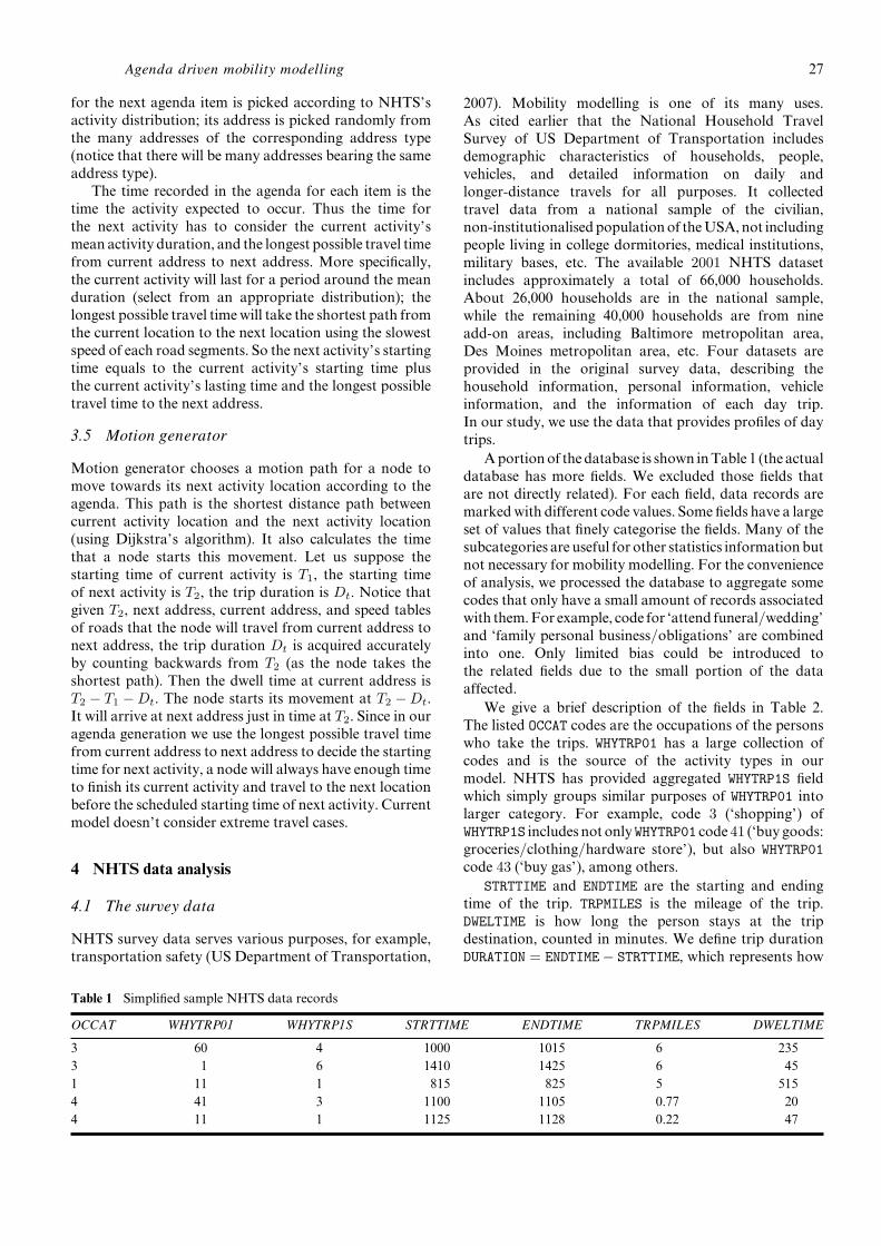
Aportionof thedatabase is shown inTable 1 (the actualdatabase has more fields. We excluded those fields thatare not directly related). For each field, data records aremarkedwith different code values. Some fields have a largeset of values that finely categorise the fields. Many of thesubcategories are useful for other statistics informationbutnot necessary for mobility modelling. For the convenienceof analysis, we processed the database to aggregate somecodes that only have a small amount of records associatedwith them.For example, code for ‘attend funeral/wedding’and ‘family personal business/obligations’ are combinedinto one. Only limited bias could be introduced tothe related fields due to the small portion of the dataaffected.

We give a brief description of the fields in Table 2.The listed OCCAT codes are the occupations of the personswho take the trips. WHYTRP01 has a large collection ofcodes and is the source of the activity types in ourmodel. NHTS has provided aggregated WHYTRP1S fieldwhich simply groups similar purposes of WHYTRP01 intolarger category. For example, code 3 (‘shopping’) ofWHYTRP1S includes not onlyWHYTRP01 code 41 (‘buy goods:groceries/clothing/hardware store’), but also WHYTRP01code 43 (‘buy gas’), among others.

STRTTIME and ENDTIME are the starting and endingtime of the trip. TRPMILES is the mileage of the trip.DWELTIME is how long the person stays at the tripdestination, counted in minutes. We define trip durationDURATION = ENDTIME − STRTTIME, which represents how

Table 1 Simplified sample NHTS data records

OCCAT WHYTRP01 WHYTRP1S STRTTIME ENDTIME TRPMILES DWELTIME

3 60 4 1000 1015 6 2353 1 6 1410 1425 6 451 11 1 815 825 5 5154 41 3 1100 1105 0.77 204 11 1 1125 1128 0.22 47

28 Q. Zheng et al.

long this trip lasts. The histograms of DURATION(trip duration), TRPMILES (trip mileage) and DWELTIME(dwell time) for different trip purposes are shown inFigures 3–5.

Table 2 Selected categories in simplified sample NHTS data

Field names Meaning Code

OCCAT occupation 1 = Sales or Service2 = Clerical or administrative

support3 = Manufacturing,

construction, maintenance,or farming

4 = Professional, managerialor technical

91 = Other

WHYTRP01 purpose 1 = Homeof a trip 11 = Go to work

41 = Buy goods: groceries/clothing/hardware store

60 = Family personalbusiness/obligations

· · ·WHYTRP1S larger 1 = Work

category 2 = Schoolof purpose 3 = Shopping

4 = Personal5 = Social6 = Others

Figure 3 Trip duration distribution (see online versionfor colours)

Figure 4 Mileage distribution (see online version for colours)

Figure 5 Dwell distribution (see online version for colours)

4.2 Data analysis

In this section, we present our analysis on the surveydata using statistics tools for the distributions of tripduration, mileage, and dwell time. All of these resultsare important for mobility modelling. We examinethe histograms obtained from the raw data presentedin Figures 3–5 (secondary distributions are removedin this analysis). We use a statistics tool calledDFITTOOL in MATLAB (MathWorks, 2007) to fitthe data to different distributions. DFITTOOL drawsCumulative Distribution Function (CDF) of the data.It also shows CDFs of those different distributionstogether in one graph, allowing us to decide whichdistribution fits the data best. In determining the closenessof fitted distributions against the real data, we useAIC (Akaike’s Information Criterion) (Burnham andAnderson, 1998) method. AIC is defined as:

AIC = −2 × (log likelihood)+ (number of parameters) × 2.

In this formula, number of parameters is the numberof parameters in the distribution. For example, thenormal distribution has two parameters, µ and σ, thus,number of parameters = 2. The log likelihood is providedby DFITTOOL as an output. So for each candidatedistribution, we can compute its AIC. The one with thesmallest AIC is the best fit for the data.

4.2.1 Trip mileage

Initial observation of the raw data shows that themileage of 94.9% trips are under or equal to 30 miles.Of the remaining records, some mileage is exceptionallylarge. Those large milage comes from long distancetravellers. The data could be helpful in a separate study toanalyse long distance motion patterns. Here, we excludeall the records whose mileages are larger than 30 miles(the threshold is selected partly due to convenience andpartly due to a reasonable good fit to the majority of thedata). Using the method we described above, we find thatthe best fit for trip mileage data is a Weibull distribution(Sa, 2003):

wα,β(x) =α

β(x/β)α−1e−(x/β)α

Agenda driven mobility modelling 29

with shape parameter α = 0.91, and scale parameterβ = 5.56. See Figure 6.

Figure 6 Fit Weibull distribution to trip mileage data

4.2.2 Trip duration

Similar to mileage data, 95.0% trips have a durationunder or equal to 50min. Of the remaining records, someduration is exceptionally large. Thus, we exclude therecords whose durations are above 50min in order tohave a reasonable good fit to the majority of the data.The best fit for trip duration is a Gamma distribution(Sa, 2003):

γa,p(x) =1

apΓ(p)e−x/axp−1

with shape parameter p = 1.87, and scale parametera = 7.87. The Gamma function is defined as Γ(p) =

∫ ∞0

e−ttp−1dt. See Figure 7.

Figure 7 Fit Gamma distribution to trip duration data

4.2.3 Dwell time

A Weibull distribution (Sa, 2003) can be used to depictthe distribution of dwell times that are under 500min(covering 92.7% data):

wα,β(x) =α

β(x/β)α−1e−(x/β)α

with shape parameter α = 0.77, and scale parameterβ = 82.17. See Figure 8.

Figure 8 Fit Weibull distribution to dwell time data

4.3 Dwell time of different activities

For the purpose of our Agenda Driven Mobility Model,we’ll take a look at the distribution and the mean oflasting time of each individual activity in WHYTRP01(notice that the distributions in previous sections areaggregated distributions). For example, for activitycode 83 (‘coffee/ice cream/snacks’), the mean timeis 26min. Negative binomial distribution describes thedwell time of each activity (with different parameters).The probability mass function of negative binomialdistribution with parameters p (0 < p < 1) and r (r > 0)is defined as:

f(k; r, p) =Γ(r + k)k!Γ(r)

pr(1 − p)k

for k = 0, 1, 2, . . . , where Γ is the gamma function.The mean values and parameters of negative binomial

distribution of some example activities are shown inTable 3.

Table 3 The mean of sample activities

MeanCode Meaning (min) r p

21 Go to school as student 355 2.38 0.00730 Medical/dental service 67 1.24 0.01840 Shopping/errands 33 0.58 0.02053 Visit friends/relatives 121 0.90 0.00780 Meals 55 1.18 0.021

5 Model analysis

In this section we use a Markov chain to analyse ourAgenda Driven Mobility Model. Using a slightly differentassumption (exponential staying at an address or location),we are able to get the limiting probabilities of a nodestaying at various addresses (or locations). The certain

30 Q. Zheng et al.

amount of predictability of a node visiting a location is animportant character of agenda.

Suppose there are n locations, noted as 1, 2, . . . ,i, . . . , n. Once the node enters location i, it will staythere for a duration obeying exponential distribution withmean 1/λi. There is also home h. The node stays athome for a duration obeying exponential distribution withmean 1/λh. There are m activities in the node’s agenda,namedA1, A2, . . . , Ai, . . . , Am. For each activity Ai, thereare several possible locations for the node to choose.For example, if the activity is dining, the node has manyrestaurants to select from. Suppose the correspondinglocation set of activityAi is Si, i = 1, 2, . . . , m. We assumenone activity in the agenda is same as another, so alllocation set Si’s are disjoint. Suppose these sets coverall locations, that is,

⋃mi=1 Si = {1, 2, . . . , n}. The size of Si

is denoted as |Si|. After the node finishes all m activities,it returns home. This procedure loops.

A continuous time Markov chain (Ross, 1983) can beset up for analysis. A state is denoted as (i, j) where iis the node’s current location, j is the number of stepsthe node has taken so far. When the chain leaves state(i, j), it will next enter state (i′, j + 1) with probabilityp(i,j),(i′,j+1). See Figure 9. If j = m, it will next enter state(h, 0) with probability one. This chain is irreducible andpositive recurrent (Ross, 1983).

Figure 9 State transition when number of steps j < m(see online version for colours)

Thus the limiting probability py = limt→∞ pxy(t), whichcan be rewritten as p(k,l) = limt→∞ p(i,j),(k,l)(t), can befound. Here p(i,j),(k,l)(t) is the probability that the chain,currently in state (i, j), will be in state (k, l) after time t.

We give an example here. Suppose a node hasan agenda consisting of only two activities: A1 andA2. Its corresponding location sets are S1 = {1, 2, 3},S2 = {4, 5}. See Figure 10. Parameters of exponentialdistributions of staying at each location are shownin the figure. We draw state transition in Figure 11.Transition rates are shown in the figure. We useKolmogorov equations (Ross, 1983) to obtain numericalresults. Figure 12 shows the state probability of each ofthe states p(h,0)(t), p(1,1)(t), p(2,1)(t), p(3,1)(t), p(4,2)(t),p(5,2)(t). Given any time t, Figure 12 gives the probabilityof staying at any of these six locations. We furthercalculate the following limiting probabilities for each

state: p(h,0) = 0.68, p(1,1) = 0.07, p(2,1) = 0.02, p(3,1) =0.03, p(4,2) = 0.11, p(5,2) = 0.09.

Figure 10 A node starting from home has an agenda consistingof activities A1 and A2. There are five locations(plus home). To conduct activity A1, the node selectone (and only one) location from location setS1 = {1, 2, 3}; to conduct activity A2, it selects onefrom set S2 = {4, 5}. The node staying at location ifor exponential time with parameter λi. It returnshome after it finishes activity A2. This procedureloops (see online version for colours)

Figure 11 Continuous time markov chain state transition(see online version for colours)

System-wide behaviour can be deducted henceforth.Recall that location sets are disjoint and no repeated visitsin one agenda circle, we take the example that there areM nodes in the network. The M nodes may visit locationi in their different step, e.g., node A in its gth step, nodeB in hth step; Or they may not visit location i at all.We use Ik as an indicator variable (Ik = 1 when node kis at location i, 0 otherwise). If the limiting probability ofnode k at location i (in its jth step) is pk

(i,j), counting theseM nodes, we have the expected number of nodes (X) atlocation i as

E[X] = E[I1 + · · · + IM ]= E[I1] + · · · + E[IM ]

=M∑

k=1

pk(i,j).

Agenda driven mobility modelling 31

Figure 12 Numerical solution: state probabilities

6 Simulation

In this section, we simulate the Agenda Driven MobilityModel (Agenda Model in short). The main objective ofthe simulation is to understand the impact of agendaand map in a simulation environment. The simulationshows that the introduction of map (with addresses) andagenda into the model has significant impact on bothnetwork topology and routing performance. The AgendaModel is implemented in a well known network simulatorQualnet (Scalable Network Technologies, 2007). Throughsimulation, we first test node movements and geographicdistributions. Then, as a case study, we simulate a MobileAd Hoc Network in an urban environment whereactivities and motion steps are generated using themodel we implemented. The nodes run routing protocolAODV (Perkins and Royer, 1999) for connectivity anddata forwarding. We evaluate topological metrics androuting performance to show mobility influence. SinceAgenda Model depicts motion and relocation of nodescontinuously over a long time, we present the results inboth short and long periods of time so as to illustrate howsocial roles and activities impact network connectivity.

In our simulation scenario, we aggregated node types tothree broader categories: the first type is employee whosefirst activity must be ‘go to work’; the second type isstudent whose first activity must be ‘go to school’; thethird type is other whose first activity could be any ofthose 35 activities in NHTS except ‘go to work’ and ‘go toschool’. The percentages of the three types are 60%, 10%and 30% respectively after the aggregation. The startingtime of the first activity of any nodes is between 8:00AMand 9:00AM. As a comparison, we also simulate RandomWaypoint Model (RWP). The Random Waypoint Modelchooses destinations randomly from the field. Nodesmovein a speed picking up randomly from the range between the

minimum and the maximum of the street speed limits thatmatch the AgendaModel. They then pause at destinationsfor a time period that is randomly picked up from theinterval between the minimum and maximum mean dwelltimes of all the addresses.

6.1 Geographic distribution

We simulate an area of 4000 m × 4000 m with 2000 nodes.There are 478 addresses in the map. The simulationruns from agenda time 08:00 to 18:00, lasting ten hours.We assume that every node will go out for lunch (mainlyaround 12:00 to 14:00), but he or she usually goes backto home for his or her dinner as one day’s activities end.We want to see that at an address, as time flows, howthe node density changes. From our simulation results, wepick two addresses to show their node density variations.The first one is a workplace, whose address is 0 4th st.with coordinates (35, 1533). We observe in Figure 13 apattern very close to real life. Employees arrive at theworkplace randomly around 08:00 to 09:00, then theystay there and work. During the lunch period, they leaveworkplace to take their lunch. The curve goes down duringthat period. After lunch they come back to work andthe curve goes up again. When its time to be off duty,people leave. Some hard-working employees may comeback again after some break. In the second address – arestaurant with address 17 3rd av. and coordinates (1168,2638), curve shown in Figure 14 – we observe a surge ofnodes during the prime lunch time and very few nodesduring other times. This is also very close to real world.On the other hand, RandomWaypoint model shows littlenode density variations (at those destinations) and alldestinations are statistically identical. The results thus arenot included here. This is because the model randomlypicks a destination,withoutmaking adifference onaddresstypes nor considering the time in a day.

Figure 13 Number of nodes at a workplace (address 0 4th st.,or (35, 1533))

Figure 14 Number of nodes at a restaurant (address 17 3rd av.,or (1168, 2638))

32 Q. Zheng et al.

6.2 Network performance

We simulate a mobile ad hoc network running routingprotocol AODV in an area of 2000 m × 2000 m. The mapis the same as in Figure 2. We set 100 nodes as beingable to communicatewhilemoving, representing the realitythat only a portion of population would be a part of themobile ad hoc network. The Distributed CoordinationFunction (DCF) of IEEE 802.11 is used at the MAClayer and the two-ray ground reflection is the radiopropagation model. The channel capacity is 2Mbps withthe default transmission range 370m in Qualnet. Thisdensity generates 11 neighbours on average which is anacceptable density. On the other hand, we intend to use aless dense network in order to observe the influence frommobility more easily. We have 5 Constant Bit Rate (CBR)flows with randomly selected sources and destinations.EachCBR sends four packets per secondwith a packet sizeof 1000 bytes. This configuration is used to generate all thefollowing results.

We show two simulation runs, one in short time periodand the other over a long time period. The short simulationruns for 900 seconds (15min), corresponding to the agendatime 8:45AM–9:00AM. Some figures below extract dataof the last 400 s from this run. The long run simulatesa 15hour period, starting from agenda time 7:45AM.A sample travel trace of seven nodes is given in Figure 15.The travel paths are the results of using Dijkstra’s shortestpath algorithm. The figure shows various routes. It alsoincludes a node that stays at its original location (the littleblack dot in the middle). Figure 16 shows the positionchanges of three nodes during the 15h period of time.Notice that the lines between points are not the real traveltraces. They simply indicate the connections between anode’s locations every twohours, starting at 8AMfromhisor her home. Here, every trace is closed – since during thisperiod, each node leaves home in the morning and returnshome at the end of the day.

Figure 15 Travel traces of seven nodes

6.2.1 Topological metrics

Through topological metrics we directly examine howthe motions generated by the Agenda model affect

nodes’ interconnections, i.e., the topology of thenetworks. We choose 75, 100 and 130 nodes respectively.The topological metrics include the average numbers ofpartitions and unreachable pairs. The calculation is basedon snapshots taken every 5 s for the short run and 5minfor the long term simulation respectively.

Figure 16 A whole day journey of three nodes. Locations arerecorded every two hours

Number of partitions. From time to time, due tothe limited transmission range, the network could bedisconnected and partitioned into many sub networks.We call such sub networks partitions. In a partition,all nodes can reach any other nodes in the same partitionover one or multiple hops. However, there is no wayto organise a route, over one-hop or multi-hops, froma node in one partition to another node in a differentpartition. LetP be a partition andD(x, y) be theminimumnumber of hops of any possible routes between node xand node y, we conclude that ∀x, y ∈ P, D(x, y) �= ∞.Our metric number of partitions describes the extent ofthis phenomenon. Specifically, suppose the number ofpartitions is n, and the partitions are P1, . . . , Pn, we have{∀x ∈ Pi, ∀y ∈ Pj | i �= j, D(x, y) = ∞}. The simulationresults are given in Figure 17. Clearly, the networkpartitions; and the number of these partitions fluctuates.The figure also shows that as network density increases,the number of partitions decreases. This is natural asnodes will have more chances to connect to other nodes.Not only that, a sparser network increases the fluctuationlevel. For example, for a 130 nodes network, the number ofpartitions is either 1 or 2; but for a 75 nodes network, thenumber of partitions fluctuates between 2 and 7. Figure 18shows the number of partitions in the long timeof 15hours.

Unreachable pairs. Because of partitioning, a pair ofnodes each belonging to a different partition can notestablish a route between them. We call such node pairsunreachable pairs. In a fully connected network of nnodes, each node can reach every other node, the totalreachable pairs is n(n − 1)/2. The unreachable pairs canbe represented as the cardinality of the set {(x, y) | x ∈ Pi,y ∈ Pj , i �= j}. Figure 19 shows the percentage of pairsthat is unreachable. It is obvious that as the number

Agenda driven mobility modelling 33

of nodes increases, the number of unreachable pairsdecreases. The curves fluctuate but the overall ratios ofunreachable pairs are kept at a low level since this isthe time period corresponding to a time interval priorto nodes’ first agenda item. Nodes are roughly evenlydistributed at their homes before they move to their firstdestinations. Compare to Figure 20, which shows the ratioof unreachable pairs in the long simulation run, the overallratio there is much higher. That is because during the longperiodof awhole day, atmany timesnodeswill concentrateat various addresses (e.g., grocery store), thus increasethe ratio of unreachable pairs (nodes at two differentaddresses are likely not to reach each other if these twoaddresses are far apart). When we compare these twofigures to the number of partitions Figures 17 and 18, wecan see that they roughly fluctuate at the same time – whenthere are more partitions, there are more pairs that cannotreach each other.

Figure 17 Number of partitions in 15min, from 8:45AMto 9:00AM

Figure 18 Number of partitions in 15h

6.2.2 Routing performance metrics

Here we examine the network performance in terms ofdelivery ratio and average path length. In order to showthe influence on the topology change of the two mobility

Figure 19 Unreachable pairs in 15min, from 8:45AMto 9:00AM

Figure 20 Unreachable pairs in 15h

models through time, we sample the metrics based on atime slot of 5 s, i.e., counting all of the packets received andsent in every 5-s time slot. Thus the delivery ratio is theratio of the number of packets received and sent during thetime slot. For the path length, we take the packets arrivedduring the slot. On average, there will be 100 packets intotal during each time slot. Since some packets may notbe generated and received within the same time slot, thedelivery ration may be larger or smaller than real cases,e.g., more than 100%. Thus, we take an average using thecurrent, the previous and the succeeding slots. Thismethodis different from earlyworkwhichmostly calculate averageat the end of the simulation. While the latter approachis common in evaluating stationary behaviour, the waywe adopt here can highlight the nonstationary behaviourof mobility better. As demonstrated in our measurement,the connectivity variations we demonstrated in previousfigures will significantly affect these two performancemetrics. Further, in comparing the two mobility models,we refer to previous research (Camp et al., 2002; Honget al., 1999) which has shown that mobility models havevital impact on routing protocol performance, withoutnecessary indications on which model tops the rest modelsnor which routing protocol reacts better to all the differentmobility models. We expect our results validate theseobservations.

34 Q. Zheng et al.

Delivery ratio. The result of delivery ratio is shownin Figure 21. The two curves vary a lot because ourmeasurements are calculated based on different time slots.Thus they are affected by the highly dynamic connectivityas shown in the previous figures. Comparing the deliveryratios of the twomodels, AgendaModel can be higher thanthat of Random Waypoint Model because when nodesin Agenda Model confine to roads, they tend to havebetter connectivity, while in Random Waypoint Modelnodes can be at any place in the area. On the other hand,AgendaModel can also createmore partitions when nodesconcentrate, leading to lower delivery ratio than that ofRandom Waypoint Model. This shows that the influenceof mobility model on routing performance is significant.The choice of mobility model in performance evaluation isimportant.

Figure 21 Delivery ratio

Average path length. Path length counts the numberof hops of the AODV routing path between the sourceand the destination for the successfully delivered packets.The average path lengths vary over time as shown inFigure 22. Same as delivery ratio, the curves vary alot for Agenda Model and Random Waypoint Model.For Agenda Model, because nodes are confined to limitedplaces (roads), the distance between them show lessarbitrary pattern than that in Random Waypoint Model.In addition, nodes in RandomWay pointModel canmoveanywhere. The routing paths then can cut corners whenpossible. This results in shorter path lengths inmany cases.

6.3 Summary

Our simulation study shows that the Agenda Modelgenerates uneven distributions of node concentrationsaround the addresses, as a demonstration of nodes’social roles and activities. Such a result is close to theobservation of a real world. The direct influence ofthe geographic concentration is the partitioning of thenetwork. The partition fluctuates as time passes and asnodesmove toparticipate different activities.Wealso showthat the use of map (with addresses) and agenda has asignificant impact on routing protocol performance, using

RandomWaypoint Model as a comparison. It shows thatdifferent mobility models would diverge on predicting theperformance of the same routing protocol. This validatesthe results from early study (Camp et al., 2002; Hong et al.,1999) that the selection of mobility models is crucial foraccurate performance evaluations. By generating realisticscenarios, Agenda Model is expected to provide morerealistic results.

Figure 22 Average path length

7 Conclusions

We have presented an Agenda Driven Mobility Model.The key contribution of the work is using a person’ssocial roles and activities as a driving force for his orhermotion.We use agenda to describe a person’s activitiesand to determine his or her whereabouts. The proposedmodel is a general framework that can be used to producevarious scenarios. In the paper, we simulated an exampleof an urban area. With a comparison to a popular statisticmobility model, we show that our model is able to reducethe unrealistic randomness. The performance resultsconfirm that different mobility models affect performancedifferently. Our results suggest that social roles and agendaactivities tend to cause geographic concentrations, whichimpact network performance significantly. Agenda modelhas its advantage in producing a performance evaluationthat reflects situations in a real world. In addition to thesimulated example of an urban area, the model can beused to generate a variety of realistic scenarios, such ascampus networks where people tend to walk rather thandrive cars.

Acknowledgement

This work was supported in part by Universityof Alabama RAC 2005 award, National ScienceFoundation under Grant No. CNS#0627147 and inpart by Dr. Nuala McGann Drescher Leave Program,Affirmative Action/Diversity Committee of the Stateof New York/United University Professions JointLabor-Management Committees.

Agenda driven mobility modelling 35

References

Bai, F., Sadagopan, N. and Helmy, A. (2003) ‘Important:a framework to systematically analyze the impactof mobility on performance of routing protocols foradhoc networks’, Proceedings of INFOCOM 2003, IEEE,pp.825–835.

Boukerche, A. and Bononi, L. (2004) ‘Simulation and modelingof wireless, mobile and ad hoc networks’, in Basagni, S.,Conti, M., Giordano, S. and Stojmenovic, I. (Eds.): MobileAd Hoc Networking, IEEE/Wiley, New York, USA.

Burnham, K. and Anderson, D. (1998) Model Selection andInference: A Practical Information-Theoretic Approach,Springer-Verlag, New York.

Camp, T., Boleng, J. and Davies, V. (2002) ‘A survey ofmobility models for ad hoc network research’, WirelessCommunications and Mobile Computing (WCMC), Vol. 2,No. 5, pp.483–502.

Choffnes, D.R. and Bustamante, F.E. (2005) ‘An integratedmobility and traffic model for vehicular wireless networks’,Proceedings of the 2nd ACM International Workshop onVehicular Ad Hoc Networks VANET ’05, ACM, Cologne,Germany, pp.69–78.

Herrmann, K. (2003) ‘Modeling the sociological aspects ofmobility in ad hoc networks’, Proceedings of the 6thACM International Workshop on Modeling Analysis andSimulation of Wireless and Mobile Systems (MSWiM 03),ACM, San Diego, CA, USA, pp.128–129.

Hong, X., Gerla, M., Pei, G. and Chiang, C.C. (1999)‘A group mobility model for ad hoc wireless networks’,Proceedings of the 2nd ACM International Workshop onModeling, Analysis and Simulation of Wireless and MobileSystems (MSWiM 99), ACM, Seattle, Washington, USA,pp.53–60.

Hsu, W., Spyropoulos, T., Psounis, K. and Helmy, A.(2007) ‘Modeling time-variant user mobility in wirelessmobile networks’, Proceedings of the 26th Annual JointConference of the IEEE Computer and CommunicationsSocieties (INFOCOM), IEEE, Anchorage, Alaska,pp.758–766.

Jain, R., Lelescu, D. and Balakrishnan, M. (2005) ‘Model t:an empirical model for user registration patterns in acampus wireless lan’,MobiCom ’05: Proceedings of the 11thAnnual International Conference on Mobile Computingand Networking, ACM Press, New York, NY, USA,pp.170–184.

Jardosh, A., Belding-Royer, E., Almeroth, K. and Suri, S.(2003) ‘Towards realistic mobility models for mobilead hoc networks’, Proceedings of the 9th AnnualInternational Conference on Mobile Computing andNetworking (MobiCom), ACM, San Diego, CA, USA,pp.217–229.

Johnson, D.B. and Maltz, D.A. (1996) ‘Dynamic source routingin ad hoc wireless networks’, in Imielinski, T. and Korth, H.(Eds.): Mobile Computing, Kluwer Academic Publishers,Norwell, MA, USA.

Kim, M., Kotz, D. and Kim, S. (2006) ‘Extracting a mobilitymodel from real user traces’, INFOCOM 2006, IEEEComputer Society Press, Barcelona, Spain.

Lam, D., Cox, D. and Widom, J. (1997) ‘Teletrafficmodeling for personal communications services’, IEEECommunications Magazine, Vol. 35, No. 2, pp.79–87.

Lelescu, D., Kozat, U.C., Jain, R. and Balakrishnan, M. (2006)‘Model t++: an empirical joint space-time registrationmodel’, MobiHoc ’06: Proceedings of the Seventh ACMInternational Symposium on Mobile Ad Hoc Networkingand Computing, ACM Press, New York, NY, USA,pp.61–72.

Li, B. (2002) ‘On increasing service accessibility and efficiencyin wireless ad-hoc networks with group mobility’, WirelessPersonal Communications, Special Issue on MultimediaNetworking and Enabling Radio Technologies, Vol. 21,No. 1, pp.105–123.

MathWorks (2007)Matlab, URL: http://www.mathworks.com

Musolesi, M., Hailes, S. and Mascolo, C. (2004) ‘An adhoc mobility model founded on social network theory’,Proceedings of the 7th ACM International Workshop onModeling Analysis and Simulation of Wireless and MobileSystems (MSWiM 04), ACM, Venice, Italy, pp.20–24.

Musolesi, M. and Mascolo, C. (2006) ‘A community basedmobility model for ad hoc network research’, REALMAN’06: Proceedings of the Second International Workshopon Multi-Hop Ad Hoc Networks: From Theory to Reality,ACM Press, New York, NY, USA, pp.31–38.

Perkins, C.E. and Royer, E.M. (1999) ‘Ad-hoc on-demanddistance vector routing’, Proceedings of Second IEEEWorkshop on Mobile Computing Systems and Applications(WMCSA ’99), IEEE, New Orleans, LA, USA, pp.90–100.

Ross, S. (1983) Stochastic Processes, John Wiley & Sons,New Jersey, pp.141–183.

Royer, E.M., Melliar-Smith, P.M. and Moser, L.E. (2001)‘An analysis of the optimum node density for ad hocmobile networks’, Proceedings of the IEEE InternationalConference on Communications, IEEE, Helsinki, Finland,pp.857–861.

Sa, J. (2003) Applied Statistics: Using SPSS, STATISTICA, andMATLAB, Springer-Verlag, New York, pp.381–404.

Saha, A.K. and Johnson, D.B. (2004) ‘Modeling mobility forvehicular ad hoc networks’, Proceedings of the 1st ACMInternational Workshop on Vehicular Ad Hoc NetworksVANET ’04, ACM, Philadelphia, PA, USA, pp.91, 92.

Scalable Network Technologies (2007) Qualnet, URL:http://www.scalable-networks.com

Tang, L., Zheng, Q., Liu, J. and Hong, X. (2007) ‘Smart:a selective controlled-flooding routing for delaytolerant networks’, IEEE International Conference onBroadband Communications, Networks, and Systems 2007(BROADNETS 2007), IEEE, Raleigh, NC, USA.

Tuduce, C. and Gross, T. (2005) ‘A mobility model based onwlan traces and its validation’, INFOCOM 2005, IEEE,pp.664–674.

US Census Bureau (2007) Topologically Integrated GeographicEncoding and Referencing System 2007, URL: http://www.census.gov/geo/www/tiger

US Department of Transportation (2007) 2001 NationalHousehold Travel Sruvey 2007, URL: http://nhts.ornl.gov/index.shtml

36 Q. Zheng et al.

Zhang, X., Kurose, J.K., Levine, B.N., Towsley, D. andZhang, H. (2007) ‘Study of a bus-based disruption-tolerantnetwork: mobility modeling and impact on routing’,MobiCom ’07: Proceedings of the 13th Annual ACMInternational Conference on Mobile Computing andNetworking, ACM, New York, NY, USA, pp.195–206.

Zheng, Q., Hong, X. and Liu, J. (2006) ‘An agenda basedmobilitymodel’,39thAnnual SimulationSymposium, IEEE,Huntsville, AL, USA.

Zheng, Q., Hong, X. and Ray, S. (2004) ‘Recent advances inmobility modeling for mobile ad hoc network research’,Proceedings of the 42thAnnualACMSoutheast Conference(ACMSE), ACM (New York, NY, USA), Huntsville, AL,USA, pp.70–75.