Quick Response Procurement

8/13/2019 Quick Response Procurement

http://slidepdf.com/reader/full/quick-response-procurement 1/17

International Journal of Production Research,

2007, 1–16, iFirst

Quick response procurement cost control strategy

for fabric manufacturing

H. YAN*y, S.-L. TANGy and G. YENz

yDepartment of Logistics, The Hong Kong Polytechnic University, Hong Kong

zFountain Set (Holdings) Ltd., Hong Kong

(Revision received December 2006)

This paper considers a material management decision making problem with

information revision of a fabric manufacturer, facing highly uncertain materialsupply and quick response demand. We construct a model by analysing thedecision process, derive the optimal solution and study the interaction amongfactors through a practical data based computational simulation. The demandinformation, in terms of estimated volume, modifiable order, and orderconfirmation respectively, is provided by the final buyer to the fabricmanufacturer in consecutive time periods. We investigate normal and urgentraw material (yarn) purchasing costs, holding cost, overstock salvage cost, as wellas availability of raw materials for urgent order. The model for a single item isthen extended to that for multiple items with the capacity constraint. The researchshows that a fabric manufacturer plays a critical role in operations efficiencyand overall cost control in a typical apparel supply chain, and reveals the cost

trade offs between purchasing and inventory under this special businessenvironment.

Keywords: Quick response; Inventory; Supply chain management; Textileindustry

1. Introduction

In a typical supply chain in the textile industry, particularly in a developing industrial

region, a fabric manufacturing company often needs to deal with a large number

of both upstream yarn providers and downstream garment manufacturerssimultaneously. A large final buyer, usually representing a brand name or retailer

chain, provides and confirms demand data in consecutive time periods during the

manufacturing process. The difficulties faced by the fabric manufacturer are thus:

the fabric manufacturer must be capable of a quick response, since it always receives

the demand order from the final buyer very late, which leaves a tight lead time for

production. In addition, both the material quality and price at the supply side is

often noticeably unstable. To cope with the quick response requirement, the fabric

manufacturer needs to purchase a certain amount of material (yarn) based on general

business experience and informal information exchange with the final buyer before

the order arrives. Such an early purchase not only gives the fabric manufacturer a

*Corresponding author. Email: [email protected]



reasonable production preparation period but also provides room for quality

material searching and better price bargaining. When the integrated demand order is

given by the final buyer, the fabric manufacturer then adjusts the material inventory

accordingly by purchasing more and starts the production. Such a demand order,

however, needs to be confirmed by the final buyer within a pre-agreed time period,since the apparel market is highly uncertain. Therefore, the fabric manufacturer

often needs to buy at a higher price if the inventory is short, or to deal with the over

inventory with a salvage cost.

Due to the long history of the textile industry and its vast influence on the global

economy, extensive researches have been conducted in the area of inventory

management related to the apparel-textile supply chain (e.g. Hunter and Valentino

1995, Chandra and Kumar 2000, Kilduff 2000, King et al . 2000a,b, Raman and Kim

2002). Based on the observation on the significant demand uncertainty in the final

market faced by the final buyers (retailers or brands), most research has focused on

the final buyers’ inventory or production management problems involving demand

uncertainty, limited sales season, and early sales information.

Fisher and Raman (1996) modelled and analysed the decisions for a fashion

skiwear firm (a brand) under the quick response requirement. Based on the

assumption that there is a production capacity limit in the second period, they

minimized the overstock and understock costs at the end of the sales season. Iyer and

Bergen (1997) examined the impact of a channel view on quick response for the

fashion industry. They applied the Bayesian model to update the demand forecast at

the end of the first period, and analysed a situation in which both the manufacturer

and the retailer can benefit from quick response. A Bayesian model requires

confirmed demand information collected in the initial period which, however, is

clearly unavailable in our problem. Fisher et al . (1997) analysed a certain set of factors that can improve quick response capability and quantified the relationship

between the expected stockout and markdown costs, without considering the holding

cost and the purchasing cost increased in the later period. Fisher et al . (2001) studied

the two-period inventory control problem of a short lifecycle product retailer to

determine the retail product initial and replenishment order quantities that minimize

the cost of lost sales, back orders and over orders. The cost items they considered are

similar to the additional purchasing cost for express, leftover, and holding cost

during the season in our model. We further consider the availability of the qualified

material in the later periods.

Sethi et al . (2001) investigated a periodic review inventory control problem withtwo delivery modes, information updates, and fixed ordering cost. They developed

a dynamic program for characterizing the optimal policy for the finite-horizon

problem. Raman and Kim (2002) studied the impact of varying inventory holding

cost and production reactive capacity on the overstock and understock cost and

the value of increasing reactive capacity for a school uniform manufacturer. They

assumed that the demands received in all periods are not modifiable and that

the additional cost for urgent production does not occur. Yan et al . (2003) analysed

the trade-off between information accuracy and delivery cost. Choi et al . (2005)

compared the quick response policy with two information update models: with the

revision of mean and the revision of both mean and variance. The results suggestthat the latter one can provide more details to analyse the significance of the

information update process. They also showed that the impacts of quick response are

2 H. Yan et al.



influenced by the choice of different pre-seasonal products as observation targets.

Villegas and Smith (2006) used a real demand data of a multinational food and

beverage company in the simulation to illustrate how safety inventory of advanced

planning system influences the variation in production and distribution order

quantities.Most of the research work in apparel supply chains is concentrated in garment

manufacturers or retailers, and the garment inventory is the most critical issue in the

overall cost control. Investigation on the fabric manufacturing is rare. However,

the recent trend in the industry is of product diversification with small production

batch size. The scale of garment manufacture has become smaller while the number

of garment manufacturers has increased, particularly in developing industrial

regions. On the other hand, fabric manufacturers provide integration in both scale

and scope to enhance the operational efficiency and economics of scale and play key

roles in the cost control of the apparel supply chain. The problem faced by the fabric

manufacturer is highly intricate since the manufacturer is not directly linked with themarket and needs to deal with a large number of its material suppliers and product

receivers.

In this paper, analytical models are constructed according to the practical

decision-making process. We obtain the optimal solution and study the interaction

among operational factors through a practical data-based computational simulation.

The basic model is constructed concerning a single fabric item from a single final

buyer. The demand information is in the following forms.

. The first piece of information is from the informal communication with the

final buyer.

. The second one is from an integrated formal demand order for the season,but the order is allowed to be revised within a mutually agreed period.

. The third one is an order confirmation which must be completed in time by

the manufacturer.

The information is thus provided to the fabric manufacturer in three consecutive

time periods.

The fabric manufacturer then needs to place an initial order of raw materials to

prepare the production and adjust the inventory two times according to changes of

demand information. We model the raw material procurement problem to determine

the initial safety inventory level. This level is based on the initial estimation of the

final product demand and the availability of raw material in later periods, in order to

minimize holding, urgent purchasing, and salvaging costs. It should be noted that

once the final product demand information is confirmed, the manufacturer must

meet the client’s requirement in time. At that time the quantity of urgent material

purchasing or the leftover can be determined by inspecting the material inventory

level. This is thus a stochastic dynamic problem constrained by the availability of the

qualified raw material in the latter period.

This single item basic model is then extended to that for multiple fabric orders

with a fixed capacity constraint, usually caused by warehouse limitations or financial

conditions. This phenomenon is often observed when the safety inventories, usually

more than half of the total volume during the season, are placed according to the

initial demand estimation.

Quick response procurement cost control strategy for fabric manufacturing 3



A practical data-based computational simulation is conducted. The relationship

between optimal expected total cost (the sum of holding cost, urgent purchasing costand leftover cost) and parameters such as unit holding cost, urgent unit purchasing

cost, unit leftover cost, limit of available qualified raw materials, and accuracy of

demand order information, are formulated and tested. This research reveals the

overall cost tradeoffs between purchasing and inventory under this special business

environment and provides a proper decision-making framework for the industry.

2. Modelling framework for single fabric order

Consider a production period during the time point [t0, t3], illustrated as figure 1 fora single item of a single sales order. In this work, we assume that the time points are

fixed given the initial point t0. We call the yarn inventory policy a (S 0, Q1, Q2) model.

2.1 Demand estimation at time point t0

About 10 months before the garment goods appear on shelves, denoted by time

point t0 in figure 1, the fabric manufacturer needs to make its estimation on the

total volume of fabric needed in the corresponding season, based on its business

experience and estimated demand (P) from the final buyer. The fabric

manufacturer must determine the safety inventory level S 0 and place an orderfrom the yarn spinning mills at this point to ensure that the order is received

before time t1. At t1, it receives the demand order from the final buyer and starts

the production. Note that this estimated demand is highly uncertain and can

vary in the following period. The demand order is sometimes cancelled by the

buyer due to market competition.

To determine the safety inventory level, the fabric manufacturer has to consider

two folds of the expected cost. On the one hand, it pays for yarn procurement,

transportation, storage, insurance and others. Due to the great uncertainty of

estimation, overstock may occur. The yarn left at the end of the production season

would be salvaged at a low price. On the other hand, if the safety inventory levelcannot meet the demand of the following periods, a yarn trader is an urgent material

source for the fabric manufacturer. The yarn trader makes its profit by committing

Figure 1. Yarn ordering time line (t0, t3) concerning a fabric manufacturer.

4 H. Yan et al.



to certain inventory or future shipments to fabric manufacturers at a premium as

reward for bearing the inventory risk.

The reduction of lead time for an urgent yarn source is associated with a higher

price premium and logistics cost. More importantly, the characteristics or quality of

cotton yarn produced in different geographical locations might differ considerablydue to the quality of cotton fibre as well as the spinning technology. The availability

of quality stock from yarn traders imposes further constraints on the time required to

source the appropriate yarn in the required quantity.

2.2 Demand order received at time t1

At time t1, the final buyer directly, or through garment manufacturers, places

an order, denoted by R1 in figure 1, to the fabric manufacturer. However, it is

a common practice in the industry that such an order is allowed to be modified

within a certain range of quantities without any penalty before time t2, attributed to

the uncertainty of customer demand in the final garment market. But the demand

variation is smaller than before.

When the inventory cannot meet the modifiable order, the fabric manufacturer

would not have sufficient time to reorder from yarn mills and has to source

additional material from the nearby yarn traders, with a higher unit purchasing cost

p1 compared with p0 from yarn millers, for the limitation of lead time. The logistic

cost at this time has no obvious difference from that at t0. The higher purchasing cost

is mainly caused by a higher price premium from the yarn traders. The manufacturer

needs to determine the required inventory level and ordering quantity, denoted by S 1and Q1 respectively, with the new information. Similar to the situation at t0, the

overstock would cause more holding cost and salvage cost, and the understockwould cause further urgent purchasing cost. The inventory level S 1 determined at this

time is compared with the existing yarn inventory S 0. If S 1 does not exceed S 0,

no order is placed. Otherwise, an additional order Q1 would be placed to yarn

traders. Furthermore, the availability of qualified yarn is also limited.

2.3 Order confirmation at time t2

At time t2, the final buyer can update the garment demand information according to

the fresh sales data, and confirm the total fabric order, denoted by R2, to the fabric

manufacturer. Following the confirmed order, the manufacturer makes a furtheryarn ordering, denoted by Q2, with a higher cost p2 compared to p1. The high

purchasing cost at this time is mainly caused by the high logistic cost due to the tight

lead time. Note that generally there is no need to consider the limit of the available

yarn quantity from yarn traders, since in most cases, the ordering quantity Q2 of the

fabric manufacturer is much smaller than Q1.

If the manufacturer only places one order before time point t2, this problem is a

simple one-period newsvendor model and can be solved by the standard newsvendor

solution. In this problem, the order can be placed at both t0 and t1. Thus it is a

two-period dynamic program subject to the limited available material with three sets

of demand information. The decision process involves determining S 0 at t0 when thedemand estimation is made, Q1 at t1 when the order is placed and Q2 at t2 when

the order is confirmed, to minimize the sum of expected inventory holding cost,




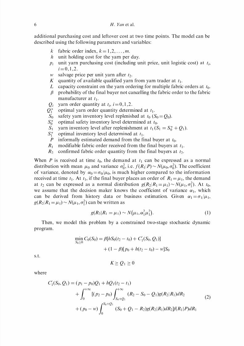
additional purchasing cost and leftover cost at two time points. The model can be

described using the following parameters and variables:

k fabric order index, k ¼ 1,2, . . . , m.

h unit holding cost for the yarn per day.

pi unit yarn purchasing cost (including unit price, unit logistic cost) at ti ,

i ¼ 0,1,2.

w salvage price per unit yarn after t2.

K quantity of available qualified yarn from yarn trader at t1.

L capacity constraint on the yarn ordering for multiple fabric orders at t0.

probability of the final buyer not cancelling the fabric order to the fabric

manufacturer at t1.

Qi yarn order quantity at ti , i ¼ 0,1,2.

Q 1 optimal yarn order quantity determined at t1.

S 0 safety yarn inventory level replenished at t0 (S 0 ¼ Q0).

S 0 optimal safety inventory level determined at t0.S 1 yarn inventory level after replenishment at t1 (S 1 ¼ S 0 þ Q1).

S 1 optimal inventory level determined at t1.

P informally estimated demand from the final buyer at t0.

R1 modifiable fabric order received from the final buyers at t1.

R2 confirmed fabric order quantity from the final buyers at t2.

When P is received at time t0, the demand at t1 can be expressed as a normal

distribution with mean 0 and variance 20 , i.e. f (R1|P) N (0, 20 ). The coefficient

of variance, denoted by 0 ¼ 0/0, is much higher compared to the information

received at time t1. At t1, if the final buyer places an order of R1 ¼ 1, the demand

at t2 can be expressed as a normal distribution g(R2|R1 ¼ 1) N (1, 21 ). At t0,

we assume that the decision maker knows the coefficient of variance 1, which

can be derived from history data or business estimation. Given 1 ¼ 1/1,

g(R2|R1 ¼ 1) N (1, 21 ) can be written as

gðR2jR1 ¼ 1Þ N 1, 212

1

: ð1Þ

Then, we model this problem by a constrained two-stage stochastic dynamic

program.

minS 00

C 0ðS 0Þ ¼ ½hS 0ðt2 t0Þ þ C 01ðS 0, Q1Þ

þ ð1 Þ½ p0 þ hðt2 t0Þ wS 0

s.t.

K Q1 0

where

C 01ðS 0, Q1Þ ¼ ð p1 p0ÞQ1 þ hQ1ðt2 t1Þ

þ

Z þ1

0

½ð p2 p0Þ

Z þ1

S 0þQ1

ðR2 S 0 Q1Þ gðR2jR1ÞdR2

þ ð p0 wÞ

Z S 0þQ1

0

ðS 0 þ Q1 R2Þ gðR2jR1ÞdR2 f ðR1jPÞdR1

ð2Þ

6 H. Yan et al.



where hS 0(t2 t0) represents the holding cost of raw materials during the whole

season if the fabric manufacturer purchase material from yarn mills at t0. C 01ðS 0, Q1Þ

represents the expected cost after t1. It includes the additional purchasing cost from

the trader at t1, holding cost, expected overstock cost and understock cost at the end

of the season. [ p0 þ h(t2 t0) w] S 0 represents the cost of raw materials purchasedat t0 if the final buyer cancels the total fabric order at t1. Therefore, at t0, the

objective is to choose S 0 to minimize the total expected cost C 0(S 0).

With a lengthy work, C 0(S 0) could be shown convex on S 0 0. A simulation

method is developed to solve program (2) in section 4.

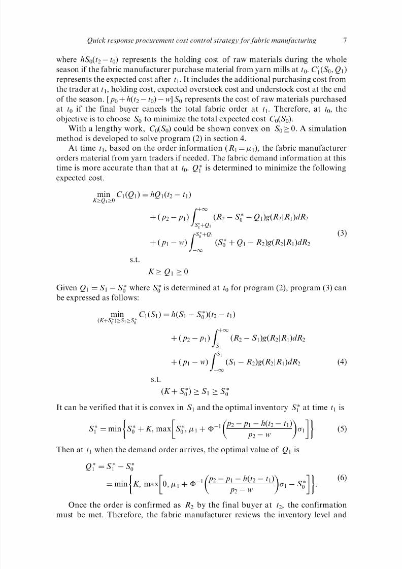
At time t1, based on the order information (R1 ¼ 1), the fabric manufacturer

orders material from yarn traders if needed. The fabric demand information at this

time is more accurate than that at t0. Q 1 is determined to minimize the following

expected cost.

minK Q10

C 1ðQ1Þ ¼ hQ1ðt2 t1Þ

þ ð p2 p1Þ

Z þ1

S 0

þQ1

ðR2 S 0 Q1Þ gðR2jR1ÞdR2

þ ð p1 wÞ

Z S 0

þQ1

1

ðS 0 þ Q1 R2Þ gðR2jR1ÞdR2

s:t:

K Q1 0

ð3Þ

Given Q1 ¼ S 1 S 0 where S 0 is determined at t0 for program (2), program (3) can

be expressed as follows:

minðK þS

0 ÞS 1S

0

C 1ðS 1Þ ¼ hðS 1 S 0 Þðt2 t1Þ

þ ð p2 p1Þ

Z þ1

S 1

R2 S 1ð Þ g R2jR1ð ÞdR2

þ ð p1 wÞ

Z S 1

1

ðS 1 R2Þ gðR2jR1ÞdR2 ð4Þ

s:t:

ðK þ S 0 Þ S 1 S 0

It can be verified that it is convex in S 1 and the optimal inventory S 1 at time t1 is

S 1 ¼ min S 0 þ K , max S 0 , 1 þ 1 p2 p1 hðt2 t1Þ

p2 w

1

ð5Þ

Then at t1 when the demand order arrives, the optimal value of Q1 is

Q 1 ¼ S 1 S 0

¼ min K , max 0, 1 þ 1 p2 p1 hðt2 t1Þ

p2 w

1 S 0

:

ð6Þ

Once the order is confirmed as R2 by the final buyer at t2, the confirmation

must be met. Therefore, the fabric manufacturer reviews the inventory level and




determines whether it needs additional yarn timely, with the highest purchasing cost

during the season. The yarn order quantity is expressed

Q2 ¼ maxð0, R2 S 0 Q 1 Þ: ð7Þ

3. Modelling for multiple fabric orders

In a real situation, the fabric manufacturer is often confronted with the case of

multiple fabric orders received simultaneously. The sum of order quantities for each

order often conflicts with the available capacity. In this section, from the single item

purchasing model, we construct a model under multiple fabric orders with capacity

constraints. The model assumes that at time t0 there is a capacity constraint, denoted

by L on the yarn purchasing. But, there are no constraints at time t1 and t2, since

more than half of the total raw materials required by each fabric order during theseason are purchased at t0. The fabric manufacturer usually clearly observes the

capacity limitation at t0, which may be caused by either warehouse capacity or

financial limit. It is consistent with the industrial situation we surveyed.

Consider m fabric item orders, all the related variables and parameters used in the

model above are added an index k (k ¼ 1,2, . . . , m), to indicate a particular order k.

At time t0, the fabric manufacturer has to deal with m fabric orders received from the

final buyers. We model the problem as

min

mk¼1

S k0L, S k00C 0ðS 10, S 20, . . . , S m0Þ ¼ X

m

k¼1

C k0ðS k0Þ

¼Xm

k¼1

k hkS k0 t2 t0ð Þ þ C 0k1 S k0, Qk1ð Þ

þ ð1 kÞ pk0 þ hkðt2 t0Þ wk½ S k0

ð8Þ

s.t.

0 Qk1 K k

Xm

k¼1

S k0 L

where

C 0k1ðS k0, Qk1Þ ¼ ð pk1 pk0ÞQk1 þ hkQk1ðt2 t1Þ

þ

Z þ1

0

pk2 pk0ð Þ

Z þ1

S k0þQk1

Rk2 S k0 Qk1ð Þ g Rk2jRk1ð ÞdRk2

þ pk0 wkð Þ

Z S k0þQk1

0

S k0 þ Qk1 Rk2ð Þ g Rk2jRk1ð ÞdRk2

f Rk1jPkð ÞdRk1

To solve (8), we first solve program (2) for each individual item and get S k0,

k ¼ 1,2, . . . , m. Then the approximating optimal solution of (8) is obtained by

a heuristics described in the next section.It is often observed in practice more than one fabric order requiring the same type

of yarn. Let z be the number of types of yarn used by m fabric orders, and l be a

8 H. Yan et al.



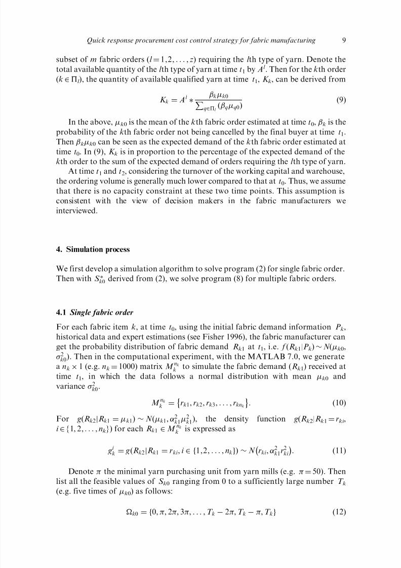
subset of m fabric orders (l ¼ 1,2, . . . , z) requiring the l th type of yarn. Denote the

total available quantity of the l th type of yarn at time t1 by Al . Then for the kth order

(k 2l ), the quantity of available qualified yarn at time t1, K k, can be derived from

K k ¼ Al kk0P

q2l ðqq0Þ ð9Þ

In the above, k0 is the mean of the kth fabric order estimated at time t0, k is the

probability of the kth fabric order not being cancelled by the final buyer at time t1.

Then kk0 can be seen as the expected demand of the kth fabric order estimated at

time t0. In (9), K k is in proportion to the percentage of the expected demand of the

kth order to the sum of the expected demand of orders requiring the l th type of yarn.

At time t1 and t2, considering the turnover of the working capital and warehouse,

the ordering volume is generally much lower compared to that at t0. Thus, we assume

that there is no capacity constraint at these two time points. This assumption is

consistent with the view of decision makers in the fabric manufacturers weinterviewed.

4. Simulation process

We first develop a simulation algorithm to solve program (2) for single fabric order.

Then with S k0 derived from (2), we solve program (8) for multiple fabric orders.

4.1 Single fabric order

For each fabric item k, at time t0, using the initial fabric demand information Pk,

historical data and expert estimations (see Fisher 1996), the fabric manufacturer can

get the probability distribution of fabric demand Rk1 at t1, i.e. f (Rk1|Pk) N (k0,

2k0). Then in the computational experiment, with the MATLAB 7.0, we generate

a nk 1 (e.g. nk ¼ 1000) matrix M nk

k to simulate the fabric demand (Rk1) received at

time t1, in which the data follows a normal distribution with mean k0 and

variance 2k0.

M nk

k ¼ rk1, rk2, rk3, . . . , rknk

: ð10Þ

For gðRk2jRk1 ¼ k1Þ N ðk1, 2k12

k1Þ, the density function g(Rk2|Rk1 ¼ rki ,

i 2 {1, 2, . . . , nk}) for each Rk1 2 M nk

k is expressed as

gi k ¼ g Rk2jRk1 ¼ rki , i 2 1,2, . . . , nkf gð Þ N rki , 2

k1r2ki

: ð11Þ

Denote the minimal yarn purchasing unit from yarn mills (e.g. ¼ 50). Then

list all the feasible values of S k0 ranging from 0 to a sufficiently large number T k(e.g. five times of k0) as follows:

k0 ¼ f0, , 2, 3, . . . , T k 2, T k , T kg ð12Þ




Denote S j k0 as the j th item of k0. With given S

j k0 and gi

k, we employ (6) to compute

the optimal value of Qk1, denoted by Qij k1. Consequently, from (2), the cost at t0 for

S j k0and Q

ij k1 is

C

ij

k0 ¼ k hkS

j

k0 t2 t0ð Þ þ C

0

k1 S

j

k0, Q

ij

k1 h i

þ 1 kð Þ pk0 þ hk t2 t0ð Þ wk½ S

j

k0: ð13Þ

Then the expected cost at t0 for a given S j k0 is calculated by averaging C

ij k0,

i ¼ 1, 2, . . . , nk as follows:

C k0 S j k0

¼

1

nk

Xnk

i ¼1

C ij k0: ð14Þ

Compute C k0ðS j k0Þ for all the items in k0, and find S k0 which minimize the

expected cost at time t0, i.e.

C k0

S k0

¼ minS j

k02k0

C k0

S j

k0 : ð15Þ

4.2 Multiple fabric orders with capacity constraint

Based on the optimal safety inventory level for single item, i.e. S k0, we consider the

solution to multiple items with the capacity constraint. With S k0, k ¼ 1,2, . . . , m,

we examine whetherPm

k¼1 S k0 exceeds the capacity limit L. If the capacity is

exceeded, we compare ½C k0ðS k0 Þ C k0ðS k0Þ for k ¼ 1,2, . . . , m and S k0 > ,

where is yarn purchasing unit from yarn mills, choose S k00 that minimizes the cost

increase, and then replace S k00 by S k00 . Repeat this procedure untilPm

k¼1 S k0

equal to or less than L. By this way, we get the optimal safety inventory level, i.e. S k0,

k ¼ 1,2, . . . , m, under the capacity constraint.

5. Computational results

This section implements the simulation solution. The goal is to understand the

relationships between the optimal expected total cost (the sum of holding cost,

additional purchasing cost for express and leftover cost) and parameters such as unitholding cost, additional unit purchasing cost for express, unit leftover cost, limit

of available qualified raw materials, and the accuracy of the information. The

experiment data is obtained from a Hong Kong-based fabric manufacturing

company, company F , located on the Chinese mainland.

5.1 Experiment for single fabric order

To analyse the relationships between cost and parameters, let the parameter studied

vary within a certain range while fixing the values of other parameters. The basic

values of the parameters are given as follows. The time points are given as t0 ¼ 0,t1 ¼ 60, t2 ¼ 90. The demand of t1 is estimated at t0. The demand at t1 follows a

normal distribution with mean 0 ¼ 10 000 and standard deviation 0 ¼ 3000.

10 H. Yan et al.



The unit purchasing costs at these time points are p0 ¼ 10, p1 ¼ 12 and p2 ¼ 14

respectively. The unit holding cost per day and unit salvage price are h ¼ 0.012 and

w ¼ 7. Let 1 ¼ 0.05, ¼ 50 and ¼ 0.8. Finally, let the quantity of available

qualified yarn from yarn trader at t1, K ¼ 2000.

Through computation, we derive the optimal solution of S 0 (see figure 2). It isobserved that the sum of the expected cost at time t0 increases if the unit holding

cost, additional unit purchasing cost for express increases, or unit salvage price, limit

of available qualified raw material or accuracy of the information decreases.

The cross impacts of two parameters on the expected cost, and the capacity

allocation for multiple fabric orders are more useful to the decision maker because in

real situation parameters often vary together. Here we exhibit several remarkable

simulation results for analysis.

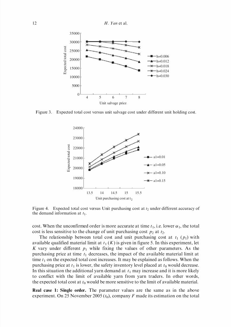
In figure 3, let the unit salvage price w vary under different unit holding cost per

day h, and values of other parameters are fixed. It shows the cross impacts of unit

holding cost and unit salvage price on the expected total cost at t0. The expected costis a function of unit salvage price, and the total cost decreases as the unit

salvage price increases. But the expected total cost is more sensitive to the unit

salvage price when the unit holding cost is lower. This suggests that when the holding

cost is low, the impact of the salvage price of leftover yarn inventory on the total cost

is notable.

In figure 4, let the unit purchasing cost at time t2 vary under different 1, and

values of other parameters are fixed. It illustrates the impact of accuracy of

unconfirmed order (1) and the unit purchasing cost at t2 ( p2) on the expected total

Figure 2. S0 versus expected total cost.




cost. When the unconfirmed order is more accurate at time t1, i.e. lower 1, the total

cost is less sensitive to the change of unit purchasing cost p2 at t2.

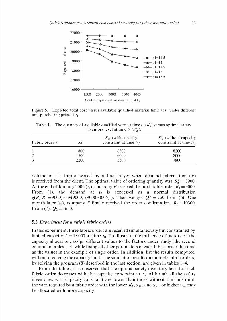
The relationship between total cost and unit purchasing cost at t1 ( p1) with

available qualified material limit at t1 (K ) is given in figure 5. In this experiment, let

K vary under different p1 while fixing the values of other parameters. As the

purchasing price at time t1 decreases, the impact of the available material limit at

time t1 on the expected total cost increases. It may be explained as follows. When the

purchasing price at t1 is lower, the safety inventory level placed at t0 would decrease.

In this situation the additional yarn demand at t1 may increase and it is more likely

to conflict with the limit of available yarn from yarn traders. In other words,

the expected total cost at t0 would be more sensitive to the limit of available material.

Real case 1: Single order. The parameter values are the same as in the above

experiment. On 25 November 2005 (t0), company F made its estimation on the total

24000

23000

E x p e c t e d t o t a l c o s t

22000

21000

20000

19000

18000

13.5 14.5

Unit purchasing cost at t2

15.514 15

a1=0.01

a1=0.05

a1=0.15

a1=0.10

Figure 4. Expected total cost versus Unit purchasing cost at t2 under different accuracy of the demand information at t1.

35000

25000

E x p e c t e d t o

t a l c o s t

15000

5000

30000

20000

10000

04 5 6

Unit salvage price

7 8

h=0.006h=0.012

h=0.018

h=0.024

h=0.030

Figure 3. Expected total cost versus unit salvage cost under different unit holding cost.

12 H. Yan et al.



volume of the fabric needed by a final buyer when demand information (P)

is received from the client. The optimal value of ordering quantity was S 0 ¼ 7900.

At the end of January 2006 (t1), company F received the modifiable order R1 ¼ 9000.

From (1), the demand at t2 is expressed as a normal distribution

g(R2|R1 ¼ 9000) N (9000, (9000 0.05)2). Then we got Q 1 ¼ 750 from (6). One

month later (t2), company F finally received the order confirmation, R2 ¼ 10300.

From (7), Q2 ¼ 1650.

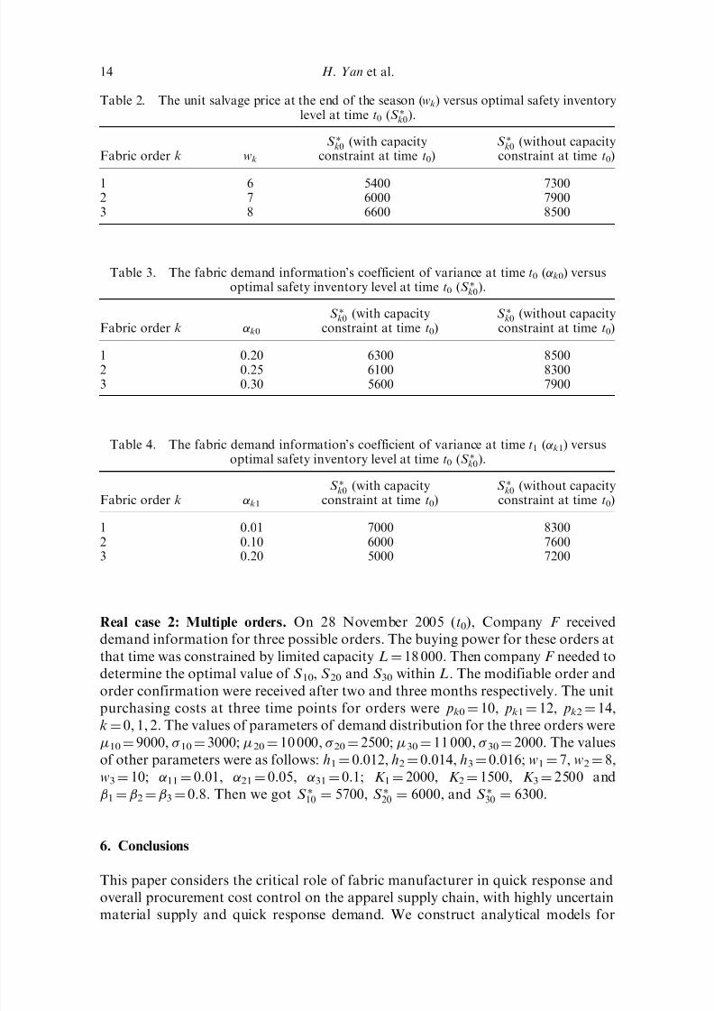
5.2 Experiment for multiple fabric orders

In this experiment, three fabric orders are received simultaneously but constrained by

limited capacity L ¼ 18 000 at time t0. To illustrate the influence of factors on the

capacity allocation, assign different values to the factors under study (the second

column in tables 1–4) while fixing all other parameters of each fabric order the same

as the values in the example of single order. In addition, list the results computed

without involving the capacity limit. The simulation results on multiple fabric orders,

by solving the program (8) described in the last section, are given in tables 1–4.

From the tables, it is observed that the optimal safety inventory level for each

fabric order decreases with the capacity constraint at t0. Although all the safety

inventories with capacity constraint are lower than those without the constraint,the yarn required by a fabric order with the lower K k, k0, and k1, or higher wk, may

be allocated with more capacity.

22000

21000

20000

E x p e c t e d t o t a

l c o s t

19000

18000

17000

16000

1500 2000 3000

Available qualified material limit at t1

3500 4000

p1=11.5

p1=13.5

p1=13.5

p1=12

p1=13

Figure 5. Expected total cost versus available qualified material limit at t1 under differentunit purchasing price at t1.

Table 1. The quantity of available qualified yarn at time t1 (K k) versus optimal safetyinventory level at time t0 (S k0).

Fabric order k K k

S k0 (with capacityconstraint at time t0)

S k0 (without capacityconstraint at time t0)

1 800 6500 82002 1500 6000 80003 2200 5500 7800




Real case 2: Multiple orders. On 28 November 2005 (t0), Company F received

demand information for three possible orders. The buying power for these orders at

that time was constrained by limited capacity L ¼ 18 000. Then company F needed to

determine the optimal value of S 10, S 20 and S 30 within L. The modifiable order and

order confirmation were received after two and three months respectively. The unit

purchasing costs at three time points for orders were pk0 ¼ 10, pk1 ¼ 12, pk2 ¼ 14,k ¼ 0, 1, 2. The values of parameters of demand distribution for the three orders were

10 ¼ 9000, 10 ¼ 3000; 20 ¼ 10 000, 20 ¼ 2500; 30 ¼ 11 000, 30 ¼ 2000. The values

of other parameters were as follows: h1 ¼ 0.012, h2 ¼ 0.014, h3 ¼ 0.016; w1 ¼ 7, w2 ¼ 8,

w3 ¼ 10; 11 ¼ 0.01, 21 ¼ 0.05, 31 ¼ 0.1; K 1 ¼ 2000, K 2 ¼ 1500, K 3 ¼ 2500 and

1 ¼ 2 ¼ 3 ¼ 0.8. Then we got S 10 ¼ 5700, S 20 ¼ 6000, and S 30 ¼ 6300.

6. Conclusions

This paper considers the critical role of fabric manufacturer in quick response andoverall procurement cost control on the apparel supply chain, with highly uncertain

material supply and quick response demand. We construct analytical models for

Table 3. The fabric demand information’s coefficient of variance at time t0 (k0) versusoptimal safety inventory level at time t0 (S k0).

Fabric order k k0



1 0.20 6300 85002 0.25 6100 83003 0.30 5600 7900

Table 2. The unit salvage price at the end of the season (wk) versus optimal safety inventorylevel at time t0 (S k0).

Fabric order k wk



1 6 5400 73002 7 6000 79003 8 6600 8500

Table 4. The fabric demand information’s coefficient of variance at time t1 (k1) versusoptimal safety inventory level at time t0 (S k0).

Fabric order k k1



1 0.01 7000 83002 0.10 6000 76003 0.20 5000 7200

14 H. Yan et al.



single item and multiple items with normal and urgent raw materials (yarn)

purchasing costs, holding cost, overstock salvage cost, as well as availability of raw

materials for urgent order. We simulate the relationship between optimal expected

total cost and related parameters. The analysis reveals the overall cost trade offs

between the purchasing and inventory under this special business environment, andprovides an insightful decision-making framework for the industry.

It can be observed in practice that several fabric orders using the same type of

yarn while the available qualified yarn is limited at time t1. The allocation policy of

this limited quantity among orders has an impact on the decision-making

of inventory. In this work the available qualified yarn at time t1 (A1) is allocated

at time t0 in proportion to the percentage of its expected demand to the sum of the

expected demand of orders using the same type of yarn (see equation (9)). Future

work can be conducted by analysing other possible allocation policies. The risk-

pooling effect can be applied in this situation. The effect of risk-pooling can be

briefly explained as that the standard deviation of the sum of the fabric orders is lessthan the sum of standard deviations of orders. Since these fabric orders are jointly

constrained by the availability of the same type of yarn at time t1, the variance of

orders can be pooled and shared among them when considering the impact of this

constraint, and the decision on inventory made at time t0 would also be changed

accordingly.

Acknowledgements

This research is partially supported by the Hong Kong Polytechnic UniversityResearch Grant A628.

References

Chandra, C. and Kumar, S., An application of a system analysis methodology to managelogistics in a textile supply chain. Sup. Chain Manage., 2000, 5, 234–245.

Choi, T.M., Li, D. and Yan, H.M., Optimal single ordering policy with multiple deliverymodes and Bayesian information updates. Comp. Oper. Res., 2004, 31, 1965–1984.

Choi, T.M., Li, D. and Yan, H.M., Quick response policy with Bayesian information updates.Euro. J. Oper. Res., 2005, 170, 788–808.

Fisher, M. and Raman, A., Reducing the cost of demand uncertainty through accurateresponse to early sales. Oper. Res., 1996, 44, 87–99.

Fisher, M., Hammond, J., Obermeyer, H. and Raman, A., Configuring a supply chain toreduce the cost of demand uncertainty. Prod. Oper. Manage., 1997, 6, 211–225.

Fisher, M., Rajaram, K. and Raman, A., Optimising inventory replenishment of retail fashionproducts. Manuf. Serv. Oper. Manage., 2001, 3, 230–241.

Hunter, N.A. and Valentino, P., Quick response—Ten years later. Int. J. Cloth. Sci. Tech.,1995, 7, 30–40.

Iyer, A.V. and Bergen, M.E., Quick response in manufacturer-retailer channels. Manage. Sci.,1997, 43, 559–570.

Kilduff, P., Evolving strategies, structures and relationships in complex and turbulent businessenvironments: the textile and apparel industries of the new millennium. J. Text. Apparel,Tech. Manage., 2000, 1, 1–9.




King, R.E., Brain, L.A. and Thoney, K.A., Control of yarn inventory for a cottonspinning plant: part 1. Uncorrelated demand. J. Text. Apparel, Tech. Manage.,2002a, 2, 1–11.

King, R.E., Brain, L.A. and Thoney, K.A., Control of yarn inventory for a cotton spinningplant: part 2. Correlated demand and seasonality. J. Text. Apparel, Tech. Manage.,

2002b, 2, 1–7.Raman, A. and Kim, B., Quantifying the impact of inventory holding cost and reactive

capacity on an apparel manufacturer’s profitability. Prod. Oper. Manage., 2002, 11,358–373.

Sethi, S.P., Yan, H.M. and Zhang, H.Q., Peeling layers of an onion: inventory model withmultiple delivery modes and forecast updates. J. Optim. Theory Appl., 2001, 108,253–281.

Villegas, F.A. and Smith, N.R., Supply chain dynamics: analysis of inventory vs. orderoscillations trade-off. Int. J. Prod. Res., 2006, 44, 1037–1054.

Yan, H., Yu, Z. and Cheng, T.C.E., A strategic model for supply chain design with logicalconstraints: formulation and solution. Comp. Oper. Res., 2003, 30, 2135–2155.

16 H. Yan et al.

Quick Response Procurement

Documents

Transcript of Quick Response Procurement