
Questioning Gender Studies on Chess · Questioning Gender Studies on Chess The most important...
28
1 Questioning Gender Studies on Chess The most important theories about gender differences in chess, are the participation rate hypothesis (Bilalic, Smallbone, McLeod & Gobet, 2009) and the natural talent hypothesis (Howard, 2014). A replication using the original data, showed that the approach set out by Bilalic et al. (2009) suffered from serious methodological problems. The results of some other studies supporting the participation rate hypothesis, have also been called into question. Howard claimed that players should be examined when at their performance limit, which they reach, on average, at 750 FIDE-rated games. While this approach was adequate, he did not control for the players’ ages. The current study focuses on players in the FIDE and German databases who were continually active between the ages of 12 and 18 years. There was a gender-specific correlation between the number of games played and the rating, which was best fitted by the logistic function. The curves for the females were shifted to lower ratings and higher numbers of games in both databases; female players dropped out of tournament chess at a younger age. In the German database, a significant proportion of them had already stopped playing tournament chess at around 14 years of age. This was not detectable for the males. The implications are discussed. In the January 2019 international chess federation (FIDE) rating list, the best 100 males were, on average, 254 points stronger than the best 100 females. This situation has not changed during the last 20 years: In January 1999, the difference was 250 points and in January 2009, the males were 239 points stronger. The causes of male superiority have also been the subject of a controversial debate among scientists. The most influential paper was that by Bilalic et al. (2009), which helped Bilalic win the Karpow-Schachakademie science award in 2009. The authors found that 96 % of the differences between females’ and males’ playing strengths could be attributed to the simple fact that
Transcript of Questioning Gender Studies on Chess · Questioning Gender Studies on Chess The most important...

1
Questioning Gender Studies on Chess
The most important theories about gender differences in chess, are the participation rate
hypothesis (Bilalic, Smallbone, McLeod & Gobet, 2009) and the natural talent hypothesis
(Howard, 2014). A replication using the original data, showed that the approach set out by
Bilalic et al. (2009) suffered from serious methodological problems. The results of some other
studies supporting the participation rate hypothesis, have also been called into question.
Howard claimed that players should be examined when at their performance limit, which they
reach, on average, at 750 FIDE-rated games. While this approach was adequate, he did not
control for the players’ ages. The current study focuses on players in the FIDE and German
databases who were continually active between the ages of 12 and 18 years. There was a
gender-specific correlation between the number of games played and the rating, which was
best fitted by the logistic function. The curves for the females were shifted to lower ratings
and higher numbers of games in both databases; female players dropped out of tournament
chess at a younger age. In the German database, a significant proportion of them had already
stopped playing tournament chess at around 14 years of age. This was not detectable for the
males. The implications are discussed.
In the January 2019 international chess federation (FIDE) rating list, the best 100 males were, on
average, 254 points stronger than the best 100 females. This situation has not changed during the
last 20 years: In January 1999, the difference was 250 points and in January 2009, the males were
239 points stronger. The causes of male superiority have also been the subject of a controversial
debate among scientists. The most influential paper was that by Bilalic et al. (2009), which helped
Bilalic win the Karpow-Schachakademie science award in 2009. The authors found that 96 % of the
differences between females’ and males’ playing strengths could be attributed to the simple fact that

2
more males than females were playing chess. This notion is called the “participation rate
hypothesis”. Bilalic et al.’s study (2009) met with broad acceptance, not only in the chess scene but
also in newspapers, magazines and social media, however, critical voices were also heard. Knapp
(2010) doubted the authors’ methodology. The English chess grandmaster Nigel Short, called
Bilalic et al.’s study (2009) “the most absurd theory to gain prominence in recent years” (Short,
2015). He raised a media storm when he stated that “men and women’s brains are hard-wired very
differently, so why should they function in the same way?” Howard (2014) claimed that males had
innate advantages in chess. This notion is called the “natural talent hypothesis”.
Vaci, Gula & Bilalic (2015) argued that the FIDE database that Howard (2014) used in his study,
“suffers from serious methodological problems”, which would explain the different results. Vaci &
Bilalic (2017) offered a version of the German database for download, which was the same one that
Bilalic et al. (2009) had used. Thus, the possibility of replicating both studies from the original data
arose. The freely available software R (R Core Team, 2018) was used for this purpose. R is an
interpreted programming language, and one of the standard tools in statistics. It is an open source
software, which is continually being upgraded by scientists all over the world and consists of a base
package and more than 10,000 additional packages for special purposes. All the graphs in this paper
were plotted using the R packages “ggplot2” (Wickham, 2016), “gridExtra” (Auguie, 2017), and
“export” (Wenseleers & Vanderaa, 2018), the latter being used to save them to JPEG files. In the
first part, Bilalic et al.’s (2009) and Howard’s (2014) studies are replicated. It is shown that female
players drop out of tournament chess earlier. The second part focuses on the relationship between
the number of games played and the players’ rating in both databases. The third part will address the
question of whether the German database is really superior to the FIDE database. Links to the
original papers discussed here are provided in the reference section.

3
Bilalic et al.’s (2009) Participation Rate Hypothesis
The German database which Vaci & Bilalic (2017) offered for download, contained 131,147 players
with a total of 2,108,908 observations. The German Chess Federation’s (DSB) DWZ system
(“Deutsche Wertungszahl”, German Evaluation Number) is based on the same principles as the
FIDE’s Elo system (Elo, 2008, originally published in 1978). Chess players are rated on a
continuous scale which ranges from about 700 DWZ or 1,000 Elo points, for the FIDE database, to
about 2,800 points for the best international grandmasters. German club players have around 1,500
DWZ points, on average. Players with 2,000 points or more are commonly considered to be experts.
Grandmasters have reached 2,500 Elo points and fulfilled some other FIDE norms. Players win or
lose rating points depending on the results of games against other rated players. Bilalic et al. (2009)
excluded all foreign players from their analyses. The total number of German players in the
database was 120,680, of which 113,651 were males and 7,029 females. This fitted well with the
figures provided by Bilalic et al. (2009), which were 113,389 and 7,013 respectively. It took me
some time to find out what observations the authors had used in their study, which were in fact, the
last entry for each player. Only when these entries were used, were the mean and standard deviation
identical to the values stated by the authors (M=1,461, SD=342). Mean and standard deviation are
the most important parameters of a normal distribution which is characterized by a Gaussian bell
curve. The standard deviation is a measure of the spread or width, of a bell curve.
The Illusion of a Common Distribution
The German magazine Spiegel online summarized Bilalic et al.’s paper (2009) as follows:
“Provided that men and women are equally smart, the difference in points between

4
the best 100 men and women should correspond to the numerical difference in size
of both groups. Actually, the researchers found hardly any difference between the
statistically expected and the real numbers of points. […] Overall, men stayed ahead,
but only by a razor-thin lead of 353 to 341 points. Therefore, 96 per cent of the
gender difference is explainable in purely statistical terms...” (Spiegel online, 2009,
translated from German)
How is the phrase “men and women are equally smart” translated into statistical language? Bilalic
et al. (2009) used the terms “shared population” and “common distribution”. This reflects what the
supporters of the participation rate hypothesis actually claim, namely that female and male ratings
belong to the same population and that differences in the extremes are only due to different sample
sizes; a bell curve of 113,000 players is simply broader than one of 7,000 players. This sounds
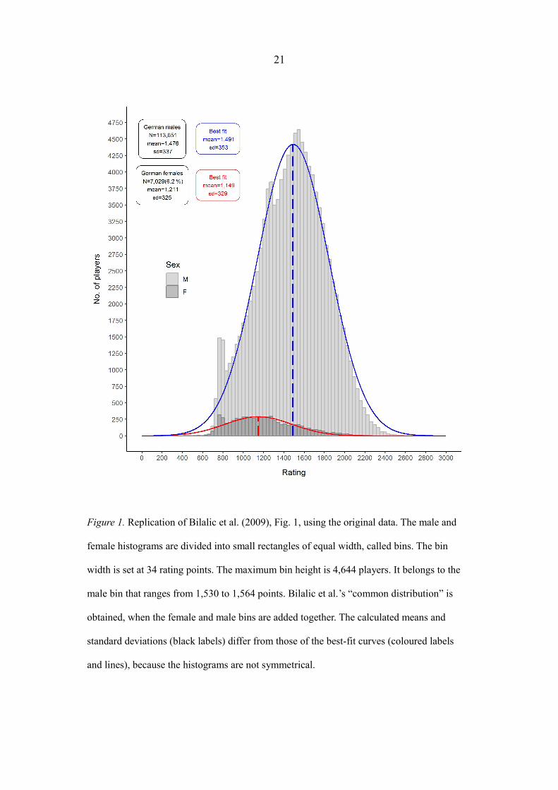
plausible. The only problem is that there is no “common distribution”, which is evident from the
histograms in Fig. 1. The calculated mean ratings for females and males differ by 265 points. The
342-point difference in the best-fit bell curves is even larger. The mean of the authors’ “common
distribution” is the weighted mean of the single populations: 1,211*7,029/120,680 +
1,476*113,651/120,680 = 1,461 (the asterisk * is the multiplication, the slash / the division sign).
The crucial point is that the female mean rating does not rise by 250 points simply because they are
in the same database as the males. Bilalic et al. (2009) assumed, as already proven, what they still
had to prove. What should have been their outcome was actually their premise, as illustrated by the
phrase “provided that men and women are equally smart” in Spiegel online’s summary. Bilalic et
al.’s (2009) argumentation was a case of circular reasoning. Moreover, the authors implicitly
assumed that the mean and standard deviation would not change if the number of female players
were multiplied. This is not guaranteed. If the old saying, that we like to do what we are good at, is
true, then the best players are already on board.

5
The two bins, mids 765 and 799, in Fig. 1, stand out from their surroundings like skyscrapers. They
are signature bins of the German database, which first appeared in 2004, when the DSB introduced
braking values and acceleration factors for players below 20 years of age. This was supposed to
help young players to improve their ratings more quickly and at the same time, prevent the ratings
of weaker players from dropping too fast. Females are younger than males on average and have
lower ratings, so they profit more from this rule. Therefore, the female signature bins are higher
than the male ones, relatively.
Approximate instead of exact. Bilalic et al. (2009) used a “simple approximation” to
calculate the expected ratings for the best 100 females and males. Their approach was a
modification of Charness & Gerchak’s method (1996), which was based on the fact that in large
samples drawn from normal distributions, the relationship between the logarithm of sample size and
the maximum value is approximately linear. According to Charness & Gerchak (1996), Fig. 1, the
slopes of the straight lines increase according to the players’ rank numbers. Bilalic et al. (2009) used
the best player’s slope provided by Charness & Gerchak (1996), for all the 100 players ranked 1-
100. Hence, there were considerable doubts about the accuracy of their method. In order to test it, it
was necessary to calculate the exact values and compare them with the authors’ approximated
values. The package “orderstats” (Sims, 2017) in R and the function “order_rnorm” were used to do
this. The expected ratings were the mean values of a large number of simulation runs. This approach
is known as Monte Carlo method. Harter’s tables (1961) were used for validation. Harter used an
ERA 1103 A mainframe computer, which according to Wikipedia, weighed 17.5 tons, to calculate
the extreme values of different normal distributions to five decimal places. It was found that
Harter’s figures (1961) could be reproduced to two decimal places, if the simulation was run
100,000 times. The question of why Bilalic et al. (2009) relied on questionable approximations even

6
though the exact values would have been easily accessible, remains. Knapp (2010) used an
SAS/IML simulation to calculate the exact values in his electronic supplementary material, which is
not available online.
Fig. 2 A shows that Bilalic et al.’s (2009) approximated values are clearly different from the exact
values. This effect is most pronounced for the higher ranks of females. Fig. 2 A also shows that both
the approximated and the exact values are unrealistic and far removed from the real values. For
example, the real rating of the best German player was 2,586 points; Bilalic et al.’s (2009)
approximation was 3,031 and the exact value 2,970. The crucial point is that the extremes of a
normal distribution can only be calculated exactly, if it is perfectly normal. “Approximately
normal” as the authors called it, is not good enough. This is best illustrated by the large free space
between the male best-fit curve and the rightmost bins in the histogram in Fig. 1. There are no
perfectly normal chess ratings in the real world. The approach used by Bilalic et al. (2009) to prove
the participation rate hypothesis, was therefore inappropriate. Charness & Gerchak’s results (1996),
who supported the participation rate account, were also unreliable for the same reason.
Bilalic et al. (2009) calculated the difference between both genders’ expected and real ratings. The
real mean rating of the best 100 males was 2,471 DWZ points, and that of the 100 best females,
2,118 points (difference 353 points). The expected mean ratings were 2,610 and 2,269 points
respectively (difference 341 points = 96 % of the real difference). The 96 % result is guaranteed as
long as the male and female mean ratings are the same, even if imaginary values are entered. If
10,000 points are taken instead of 1,461, the expected rating for the best 100 males would be 11,149
points, and that of the best 100 females, 10,808 points. The difference is again 341 points and 96 %
of the real difference. If the outcome of a study is the averaged difference of two estimated
variables, it should be viewed with scepticism. If the authors had used the exact values instead of
7
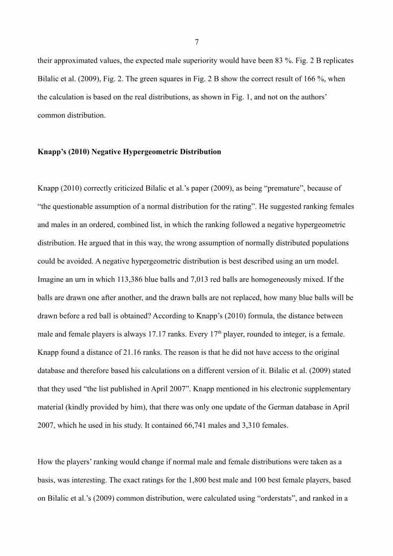
their approximated values, the expected male superiority would have been 83 %. Fig. 2 B replicates
Bilalic et al. (2009), Fig. 2. The green squares in Fig. 2 B show the correct result of 166 %, when
the calculation is based on the real distributions, as shown in Fig. 1, and not on the authors’
common distribution.
Knapp’s (2010) Negative Hypergeometric Distribution
Knapp (2010) correctly criticized Bilalic et al.’s paper (2009), as being “premature”, because of
“the questionable assumption of a normal distribution for the rating”. He suggested ranking females
and males in an ordered, combined list, in which the ranking followed a negative hypergeometric
distribution. He argued that in this way, the wrong assumption of normally distributed populations
could be avoided. A negative hypergeometric distribution is best described using an urn model.
Imagine an urn in which 113,386 blue balls and 7,013 red balls are homogeneously mixed. If the
balls are drawn one after another, and the drawn balls are not replaced, how many blue balls will be
drawn before a red ball is obtained? According to Knapp’s (2010) formula, the distance between
male and female players is always 17.17 ranks. Every 17th player, rounded to integer, is a female.
Knapp found a distance of 21.16 ranks. The reason is that he did not have access to the original
database and therefore based his calculations on a different version of it. Bilalic et al. (2009) stated
that they used “the list published in April 2007”. Knapp mentioned in his electronic supplementary
material (kindly provided by him), that there was only one update of the German database in April
2007, which he used in his study. It contained 66,741 males and 3,310 females.
How the players’ ranking would change if normal male and female distributions were taken as a
basis, was interesting. The exact ratings for the 1,800 best male and 100 best female players, based
on Bilalic et al.’s (2009) common distribution, were calculated using “orderstats”, and ranked in a

8
combined list beginning with the highest rating. The distance between the males and females was
17.10 ranks on average, and thus nearly the same as that when using Knapp’s approach (17.17). In
other words, if the sample size is large enough, the negative hypergeometric distribution simulates
two normal distributions that have identical means and standard deviations. Knapp’s (2010)
approach therefore repeated the same error as that made by Bilalic et al. (2009), which was exactly
what he had wanted to avoid.
Different Dropout Rates of Females and Males
Bilalic et al. (2009) argued that the higher female dropout rates would be “one way to avoid the
conclusion based on participation rates”, but “there is little empirical evidence to support the
hypothesis of differential drop-out rates between male and females”. The evidence will now be
presented:
Bilalic et al. (2009) used each player’s final entry in the database. This approach allows male and
female drop-out rates and ages to be compared. Their database collected data from the beginning of
the 1990s, when the current DWZ rating system replaced the Ingo system in West Germany and the
NWZ system in East Germany. It included 52,461 males and 4,067 females who had played their
last tournament in 2005 or earlier. These players had been inactive for at least one year and four
months, because the database recorded tournaments up to April 2007. Therefore, it can be assumed
that the players had concluded their tournament activity. Figures 3 A and 3 B show the ages at
which this happened. The male histogram in Fig. 3 A, is trimodal. The blue best-fit curve is
obtained by adding together the three green bell curves at any time point or age. The bell curves can
be regarded as showing the youth-, adult-, and senior fractions of players. The female adult- and
senior fractions in Fig. 3 B, are much smaller than the corresponding male fractions. In contrast to

9
the males, a fourth female fraction could be detected. These players had, on average, already
stopped playing in tournaments at 14.1 years of age (orange line in Fig. 3 B). On average, females
are below 20 years old when they play in tournaments.
Howard’s (2014) Natural Talent Hypothesis
Howard (2014) showed that in Georgia, where the percentage of female players is particularly high
and women’s chess has a high reputation, the gender differences were the same as in other
countries. He considered this to be evidence against Bilalic et al.’s participation rate account (2009).
He argued that differences in playing strength between genders, could only be studied at players’
performance limits, which they reached at 750 FIDE-rated tournament games on average. Of the
139,399 players who entered the FIDE database between July 1985 and January 2012, only 1,088
males and 115 females had played more than 750 games by January 2012. The mean male rating in
the 750-799 games category, was significantly higher than that of females (Howard, 2014, Table 1).
He therefore concluded that males must have innate advantages in chess, compared to females.
Howard’s 750-Games Limit
Updated FIDE rating lists have been published monthly since July 2012 and the FIDE offers
historical lists for download, starting from January 2001. Historical data which goes back to 1967
can be downloaded from the OlimpBase website. All these separate lists up to December 2018,
were merged into a large database with 330,781 players, among them 34,782 females, and a total of
22,559,631 observations.
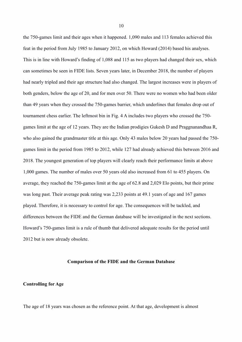
The histograms in Fig. 4 A (males) and 4 B (females), show the number of players who had passed
10
the 750-games limit and their ages when it happened. 1,090 males and 113 females achieved this
feat in the period from July 1985 to January 2012, on which Howard (2014) based his analyses.
This is in line with Howard’s finding of 1,088 and 115 as two players had changed their sex, which
can sometimes be seen in FIDE lists. Seven years later, in December 2018, the number of players
had nearly tripled and their age structure had also changed. The largest increases were in players of
both genders, below the age of 20, and for men over 50. There were no women who had been older
than 49 years when they crossed the 750-games barrier, which underlines that females drop out of
tournament chess earlier. The leftmost bin in Fig. 4 A includes two players who crossed the 750-
games limit at the age of 12 years. They are the Indian prodigies Gukesh D and Praggnanandhaa R,
who also gained the grandmaster title at this age. Only 43 males below 20 years had passed the 750-
games limit in the period from 1985 to 2012, while 127 had already achieved this between 2016 and
2018. The youngest generation of top players will clearly reach their performance limits at above
1,000 games. The number of males over 50 years old also increased from 61 to 455 players. On
average, they reached the 750-games limit at the age of 62.8 and 2,029 Elo points, but their prime
was long past. Their average peak rating was 2,233 points at 49.1 years of age and 167 games
played. Therefore, it is necessary to control for age. The consequences will be tackled, and
differences between the FIDE and the German database will be investigated in the next sections.
Howard’s 750-games limit is a rule of thumb that delivered adequate results for the period until
2012 but is now already obsolete.
Comparison of the FIDE and the German Database
Controlling for Age
The age of 18 years was chosen as the reference point. At that age, development is almost

11
completed, and players have reached about 95 % of their performance limits. The ratings are less
influenced by work or family obligations. While many players play their first tournament game at
age 18, others are active from 10 years onwards. Therefore, it is necessary to take into account the
players’ history. Only players who were continually active from 12 to 18 years of age were
analysed. Continuously active means that the number of tournament games in each of the seven
years, was greater than zero. The mean rating (hereafter rating) per year and the cumulative sum of
games (hereafter games) per year were calculated for each player. If, for example, a player had
played 100 games up to 15 years of age and 30 games at age 16, the cumulative sum of games was
130 at age 16.
Skill groups. Participants were separated by gender and ranked, either by rating or by the
number of games played, in descending order, at the age of 18, and divided into groups of 50, 100
or 200 players. For example, the M 1-100 group consisted of the 100 highest ranked males and the
F 51-100 group, of the 50 females with ranks 51 to 100. Each group’s mean rating and mean games
were calculated.
The Relationship Between Games and Rating in the FIDE Database
FIDE has lowered the rating floor continually, from its original 2,200 points, to a final 1,000 points
in 2013. The rating floor is the minimum rating a player must have to enter the database. Ratings
near the rating floor are less reliable and usually too high. In order to control for this effect, only
players who were born in the years 1998-2000, were analysed. All these players had the same rating
floor of 1,200 points, at the age of 12. There were 1,445 males and 451 females (31.2 %) who
belonged to this birth cohort and had been continuously active between the ages of 12 and 18.
12
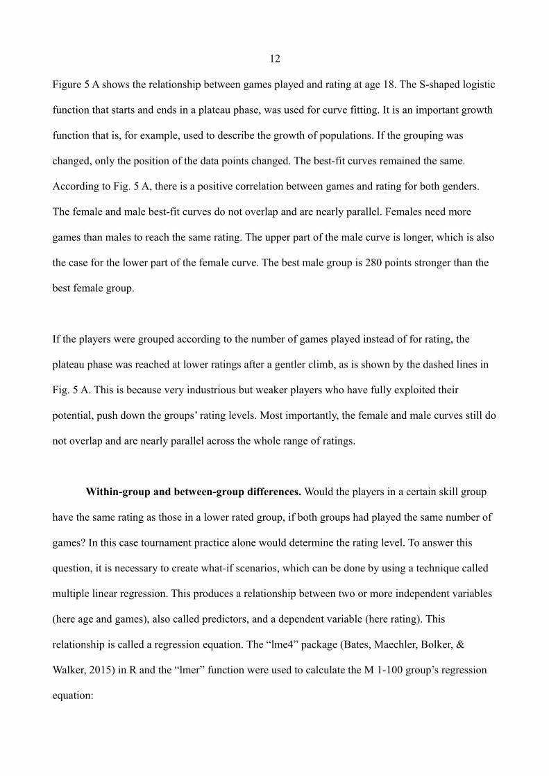
Figure 5 A shows the relationship between games played and rating at age 18. The S-shaped logistic
function that starts and ends in a plateau phase, was used for curve fitting. It is an important growth
function that is, for example, used to describe the growth of populations. If the grouping was
changed, only the position of the data points changed. The best-fit curves remained the same.
According to Fig. 5 A, there is a positive correlation between games and rating for both genders.
The female and male best-fit curves do not overlap and are nearly parallel. Females need more
games than males to reach the same rating. The upper part of the male curve is longer, which is also
the case for the lower part of the female curve. The best male group is 280 points stronger than the
best female group.
If the players were grouped according to the number of games played instead of for rating, the
plateau phase was reached at lower ratings after a gentler climb, as is shown by the dashed lines in
Fig. 5 A. This is because very industrious but weaker players who have fully exploited their
potential, push down the groups’ rating levels. Most importantly, the female and male curves still do
not overlap and are nearly parallel across the whole range of ratings.
Within-group and between-group differences. Would the players in a certain skill group
have the same rating as those in a lower rated group, if both groups had played the same number of
games? In this case tournament practice alone would determine the rating level. To answer this
question, it is necessary to create what-if scenarios, which can be done by using a technique called
multiple linear regression. This produces a relationship between two or more independent variables
(here age and games), also called predictors, and a dependent variable (here rating). This
relationship is called a regression equation. The “lme4” package (Bates, Maechler, Bolker, &
Walker, 2015) in R and the “lmer” function were used to calculate the M 1-100 group’s regression
equation:
13
Rating = 987.472 + 78.084*age + 1.818*games – 0.093*age*games (Eq. 1)
Each group has its own regression equation. The formula consists of four terms, one intercept-, one
age-, one games-, and one interaction term; this is necessary because the influence of games on
rating, depends on age. The figures in Eq. 1 are called regression coefficients. In the first step, the
software calculates age-rating curves for each participant. Individualization is achieved by random
intercepts and random slopes. This means that the intercept-coefficient and the age-coefficient in
Eq. 1, are chosen differently for each player, whereas the other two coefficients are kept constant.
The figures in Eq. 1 are the means of all the players’ coefficients. Table 1 shows group M 1-100’s
real and estimated ratings at different ages, in its upper part. The latter are obtained by entering the
player’s age and games into Eq. 1. It is possible to create a what-if scenario on the basis of Eq. 1
and to estimate group M 1-100’s mean rating by interpolation, under the assumption that its
members had played the same number of games on average, as those of group M 101-200. In this
case, group M 1-100’s ratings would still be about 90 points higher, on average, than those of group
M 101-200 (Table 1, last column).
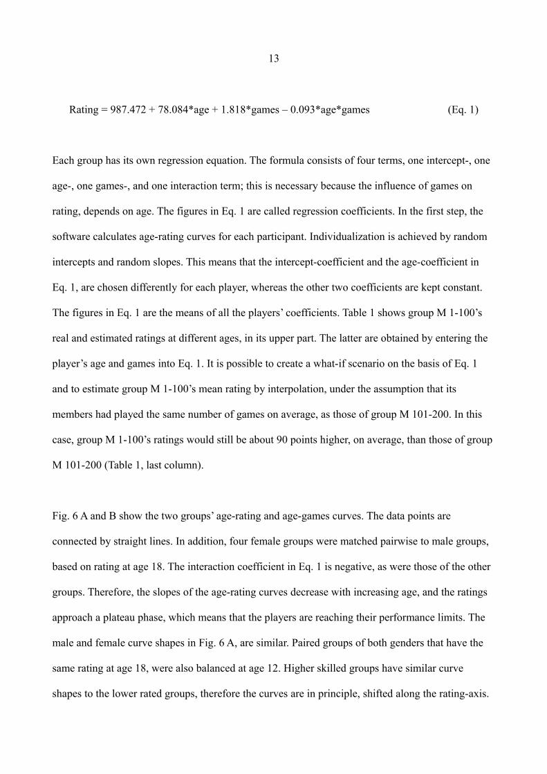
Fig. 6 A and B show the two groups’ age-rating and age-games curves. The data points are
connected by straight lines. In addition, four female groups were matched pairwise to male groups,
based on rating at age 18. The interaction coefficient in Eq. 1 is negative, as were those of the other
groups. Therefore, the slopes of the age-rating curves decrease with increasing age, and the ratings
approach a plateau phase, which means that the players are reaching their performance limits. The
male and female curve shapes in Fig. 6 A, are similar. Paired groups of both genders that have the
same rating at age 18, were also balanced at age 12. Higher skilled groups have similar curve
shapes to the lower rated groups, therefore the curves are in principle, shifted along the rating-axis.

14
Fig. 6 B shows that the female groups played more games to reach the same rating value as their
matched male groups.
To sum up, players in the same skill group who have reached their performance limit, are unable to
improve further, even if they drastically increase their number of games played. Players in higher
rated skill groups play more games than players in weaker groups, but even if they were to play the
same number of games, their ratings would still be higher. The conclusion is that strong players play
more games because they like to do what they are good at and in which they are successful. Rating
values and the number of games played are intervowen with each other. The curves in Fig. 5 A are
gender-specific. Howard’s (2014) results were in principle, confirmed. Controlling not only for
games but also for age, led to a stronger accentuation of the gender differences. His 750-games limit
is not generally valid; the number of games at which players reach their performance limit, is
positively correlated with their skill level.
The Relationship Between Games and Rating in the German Database
In the German database, 2,589 males and 362 (14.0 %) females were continuously active from 12 to
18 years of age. Foreign players were excluded. The percentage of females was only half that of the
FIDE players. The players were ranked according to rating or games (dashed lines), and grouped as
listed in the legend to Fig. 5 B. The quality of fit was worse compared to the FIDE players,
probably because it was impossible to form birth cohorts, as the number of players was too small.
There is again a positive correlation between games and rating and the male and female curves are
again nearly parallel. The best female group in Fig. 5 B, is about 360 points weaker than the best
male group. The rating range above 2,300 points is poorly represented in the German database;

15
while that below 1,500 points is poorly represented in the FIDE database. The curves in Fig. 5 B are
therefore shifted downwards, compared to those in Fig. 5 A. They are also shifted along the games-
axis. Games are measured on a different scale in the German database, but both genders are affected
in the same way. Therefore, the relative positions of the curves in Fig. 5 A and B are similar, and
only their absolute positions are different. The lower rated German players have usually played
more games than FIDE players of comparable strength, while the opposite is the case for the highest
rated players.
Fig. 6 C and D show some German players’ age-rating and age-games curves, selected according to
the same criteria as those of the FIDE players in Fig. 6 A and B. There is a tendency for German
female groups to slightly outperform matched male groups up to the age of 14 years, but then to
return to the same rating level at age 18. This phenomenon was not observed in the FIDE players,
so it is probably an artefact. In January 2001, German players who were rated below 1,300 points
profited from a staggered rating elevation. For example, players with ratings of 300 points got a
bonus of 600 points, while those rated at 1,200 points received only 50 points. Females profited
more from this rule than males, which should explain the different curve shapes.
Are National Databases Really Superior to the FIDE?
Vaci, Gula, & Bilalic (2014), Vaci Gula, & Bilalic (2015) and Vaci & Bilalic (2017) argued that the
numbers of games in the FIDE database were not correct, because national tournaments were often
not recorded. They pointed out that the FIDE players’ rating curves were truncated because of the
rating floor. They described the FIDE database as “restricted” (Vaci et al., 2015), and praised the
German database for being a “whole range database” (Vaci et al., 2014). This would explain why
“studies with the restricted FIDE-database regularly find differences between women and men in

16
skill. The studies with unrestricted national databases, however, explain these differences through
participation rates and dropout patterns.” (Vaci et al., 2015). According to them, the study of
Chabris & Glickman (2006) was one of the correct gender studies, conducted with a national
database.
Chabris & Glickman (2006) used the United States Chess Federation (USCF) database for
their gender study. The ratings in the USCF database are bimodally distributed and have two peaks
at 700-800 points and 1,500-1,600 points. The reason for this is that players who only take part in
scholar tournaments constitute a separate population which is responsible for the lower peak. The
USCF ratings are biased by a system of individual rating floors and bonus points, so that this
database would certainly not be the first choice for scientific studies. Chabris & Glickman (2006)
matched female and male players pairwise and as closely as possible, based on their ratings at the
end of 1995, age, number of rated games, and games played in the previous three years. They
identified 647 matched pairs and tracked them for 10 years, until their number had fallen below 10.
Their Fig. 3 shows that this point had already been reached after six years, in 2001. The rating
difference between males and females did not deviate significantly from zero, which the authors
took as evidence of the validity of the participation rate account. Chabris & Glickman’s study
(2006) was poorly documented and not replicable. The only information provided is that they
“focused on players who were 5 to 25 years old in 1995”. Neither the age and rating from which
their players started, nor where they ended, nor whether they played only scholar or also normal
tournaments, is known. Most importantly, the authors neglected to match according to games played
at the end of the observation period. Fig. 6 shows that by ignoring this precondition, it is not only
possible to find matched pairs but also matched groups of players, who belong to different parts of
the female and male talent pools. The crucial point is, however, that it is impossible to find females
who match the best males. Therefore, Chabris & Glickman’s paper (2006) missed the point.

17
Vaci & Bilalic (2017) used the German database to conduct a gender study and found that
“Compared with men, who need around 43 games played per year to reach DWZ ratings of 2,000,
women need approximately 33 games per year”. This result appears to debunk Howard’s study
(2014), and to confirm the participation rate account, as well as the superiority of national
databases. Vaci & Bilalic (2017) offered a “step-by-step tutorial” which included their complete R
code, so it was not difficult to see what had gone wrong. First, they neglected to exclude foreign
players from their analysis. German chess leagues have the reputation of being the strongest in the
world and attract many world class players. These top performers usually only play team
competitions in Germany. Their tournaments in other countries are not recorded, and hence their
number of games played is smaller than that of Germans of equal strength. The reanalysis showed
that only 157 of the 395 females listed in the German database who had mean ratings per year of
2,000 or more points, were Germans (labelled “D” in the database). According to the authors’
generalized additive model (GAM), they “needed” in the authors’ words, at least 48 games per year
to cross the 2,000-point limit, whereas the 238 females from other countries (labelled “A” or “E”)
achieved it in only four games.
If Vaci & Bilalic (2017) had validated their model, they would have realized that the results it
produced were drastically wrong. The model hopelessly overestimated weaker players who played
many games per year. For example, player ID 35730012 was active from 24 to 29 years of age. She
had played 40 games per year on average and reached a mean rating of 1,114 points. The model’s
estimate was 2,028 points. On the other hand, strong players were underestimated. There was a total
of 2,351 observations for females with above 2,000 points. The model found a mean rating of 1,702
points, whereas the actual mean was 2,166. In the case of males, the total number of observations
above 2,000 points, was 86,426. The fitted mean was 1,724 points, whereas the real value was

18
2,143. What is the reason for this analytical disaster? If the number of observations per player is
greater than one, it is essential to include random effects, as explained above in the Within-group
and between-group differences section. Vaci & Bilalic (2017) stated in their tutorial: “However, as
we are dealing with the big dataset, the adjustments of the random effects would be too long to run.
Therefore, we are going to apply the GAMMs on the averaged data.” Their “averaged data” did not
solve the problem, though, because 89.6 per cent of the players had been active for more than one
year. Vaci & Bilalic (2017) analysed 130,142 players with a total of 940,964 observations. The
reanalysis showed that the 32 GB of RAM in my PC were just good enough for about 1,000
players, if random intercept and random slope were included. In other words, the authors’ model
was inappropriate for large data, contradictory to what their paper title suggests. Even sophisticated
techniques lead nowhere, if basic principles are ignored. The same is true for Vaci & Bilalic’s
(2017) other GAM-models which they used to quantify birth cohort, activity, and inactivity effects.
Updating the German database is not that simple, as Vaci & Bilalic (2017) put it. The ID numbers in
their database were anonymised and although the DSB publishes weekly lists, they lack unique and
permanent IDs. Historical lists, like that offered by Vaci & Bilalic (2017), are not available to
everyone. To sum up, national databases are also restricted. The inconsistent results were due to
serious methodological problems in studies which used national databases instead of the FIDE
database. Because of its easy updatability and the wealth of data, the FIDE database is currently the
better choice in most cases.
Discussion
The participation rate hypothesis cannot explain gender differences in chess. A lot has been said and
written about the old ‘nature versus nurture’ debate, also called ‘inspiration versus perspiration’ (see

19
Howe, Davidson & Sloboda, 1998, and the open peer commentary herein for a good overview).
Talent (nature) and practice (nurture) are intervowen and not separable. Stronger players are not
only stronger because they play more tournament games, instead they play more games because
they are stronger.The number of tournament games played seems to be an adequate proxy variable
for different kinds of practice (Howard, 2013) and other environmental influences, as shown by the
consistent results in both databases, although the percentage of females was halved in the case of
the German players. The curves in Fig. 5 are gender-specific. Female players cannot exit their curve
and change over to the male curve. Females and males are different species of chess players from
the moment they start playing tournaments. What is the reason for this gender gap in playing
strength, is it natural or acquired? Chess databases provide little information about the period up to
the age of 10 years. Brain plasticity is highest in these years and then declines steadily. Talent is
actually learnable in this critical phase, at least to some extent. The most prominent example is the
Polgar sisters, who received optimal parental support and started to practice chess seriously from
about four years of age. The best female player of all time, Judit Polgar, was ranked number eight in
the world at her peak. The different drop-out rates, especially in young age, suggest that females
find chess less attractive; chess is an old war game, females have simply other interests. This could
be the reason why they lag behind during the critical period and have no chance of closing the gap
later on. However, there is virtually no experimental design for proving it scientifically. It is
premature to talk of innate talent. At present, neither which special abilities constitute chess talent,
nor which genes are involved, nor how they function, are known. Thus, there is still hope for the
egalitarians.

20
Table 1. Prediction of ratings at different numbers of tournament games played by multiple linear regression. Group M 1-100 comprises the 100 highest ranked male playersat age 18, M 101-200 the players ranked 101-200.
Group M 1-100
Age GAMES RATINGEST. RATING
EST. RATING
Mean SD Mean SDgamesM 101-200
12 135 91 2024 140 2019 199013 216 123 2129 127 2134 209914 309 148 2236 115 2241 220215 400 167 2333 102 2329 229216 490 184 2403 94 2399 236717 577 199 2451 74 2453 242718 662 213 2490 67 2490 2471
Group M 101-200
Age GAMES RATING
Mean SD Mean SD
12 93 69 1925 13613 157 91 2007 11114 234 109 2098 9815 313 124 2196 8516 390 134 2286 6817 466 142 2344 4818 528 154 2377 25
21
Figure 1. Replication of Bilalic et al. (2009), Fig. 1, using the original data. The male and
female histograms are divided into small rectangles of equal width, called bins. The bin
width is set at 34 rating points. The maximum bin height is 4,644 players. It belongs to the
male bin that ranges from 1,530 to 1,564 points. Bilalic et al.’s “common distribution” is
obtained, when the female and male bins are added together. The calculated means and
standard deviations (black labels) differ from those of the best-fit curves (coloured labels
and lines), because the histograms are not symmetrical.

22
Figure 2. (A) Comparison of Bilalic et al.’s (2009) approximate values with the exact values,
based on the authors’ common distribution. The higher the rank, the more inaccurate is the
authors’ approximation. Not only the approximate but also the exact ratings, deviate clearly
from the real values. (B) Comparison of the pairwise rating differences for the best 100
males and females. The black squares and filled triangles are identical with Bilalic et al.
(2009), Fig. 2. The green squares illustrate the correct result, based on the separate
distributions of females and males, as shown in Fig. 1.

23
Figure 3. Histograms of dropout ages from tournament chess of males (A) and females (B)
in the German database. The bin width is one year. The blue best-fit curve for males is
obtained by adding together the three green bell curves at any time point or age. The first
figure in the brackets is the mean, the second one the standard deviation of the bell curves.
An additional group of players is detectable under the red female curve, who had already
given up tournament chess at 14.1 years of age (orange line). N = normal distribution.

24
Figure 4. Ages of players in the FIDE database, at which they crossed Howard’s 750-games
limit. The bin width is one year. The number of male (A) and female (B) players has nearly
tripled in approximately the last seven years since Howard’s (2014) study. The histograms
are divided into three age ranges by two vertical lines. n = number of players in both periods.

25
Figure 5. Relationship between the cumulative sum of games and the rating of females and
males in the FIDE (A) and the German database (B) at age 18. Players, who were
continuously active from 12 to 18 years of age, were ranked by rating and grouped as shown
in the legends, beginning with the highest rating. Data points are the means of each group’s
games and rating. The red and blue lines are the male and female groups’ best-fit curves,
fitted by the logistic function. The dashed lines are obtained, when the players are grouped
for games instead of for rating. The data points are dropped, so as to not overload the plots.
Group F 401-450 for example: the 50 females ranked 401 - 450 at age 18.

26
Figure 6. Age-rating and age-games curves for some groups of FIDE (A and B) and German
players (C and D). The grouping and order of groups, beginning with the highest rating, is
identical for the rating and games curves. Four female and male groups were matched
pairwise as closely as possible, by rating at age 18. Data points are the means of games and
rating of each group. Group M 1101-1300 for example: the 200 males ranked 1101 – 1300
for rating at age 18.

27
References
Auguie, B. (2017). gridExtra: Miscellaneous Functions for “Grid” Graphics. R package version 2.3.https://CRAN.R-project.org/package=gridExtra
Bates D., Maechler M., Bolker B., & Walker S. (2015). Fitting Linear Mixed-Effects Models Using lme4. Journal of Statistical Software, 67(1), 1-48.
Bilalic, M., Smallbone, K., McLeod, P. & Gobet, F. (2009). Why are (the best) women so good at chess? Participation rates and gender differences in intellectual domains. Proceedings of the Royal Society B: Biological Sciences. 276, 1161-1165.
Chabris, C. F. & Glickman, M. E. (2006). Sex Differences in intellectual performance. Analysis of alarge cohort of competitive chess players. Psychol Sci. 17, 1040-1046.
Charness, N. & Gerchak, Y. (1996). Participation rates and maximal performance: A log-linear explanation for group differences, such as Russian and male dominance in chess. Psychol. Sci. 7, 46-51.
Elo, A. E. (2008). The Rating of Chessplayers, Past & Present. Bronx, NY: Ishi Press International. (originally published in 1978).
Harter, H. L. (1961). Expected values of normal order statistics. Biometrika 48, 151-165.
Howard, R. W. (2013). Practice other than playing games apparently has only a modest role in the development of chess expertise. British Journal of Psychology, 104, 39-56.
Howard, R. W. (2014). Gender differences in intellectual performance persist at the limits of individual capabilities. J. Biosoc. Sci. 46, 386-404.
Howe, M. J. A., Davidson, J. W., & Sloboda, J. A. (1998). Innate talents: Reality or myth? Behavioral and Brain Sciences 21, 399-407.
Knapp, M. (2010). Are participation rates sufficient to explain gender differences in chess performance? Proceedings of the Royal Society B: Biological Sciences. 277, 2269-70.
OlimpBase, Bartelski, W. (2019), Elo lists 1971-2001. Retrieved from http://www.olimpbase.org/Elo/summary.html
R Core Team (2018). R: A language and environment for statistical computing. R Foundation for Statistical Computing, Vienna, Austria. URL https://www.R-project.org/.
Short, N., (2015). Vive la Difference. New in Chess (2/2015). Retrieved from https://en.chessbase.com/post/vive-la-diffrence-the-full-story
Sims, C. (2017). orderstats: Efficiently Generates Random Order Statistic Variables. R package version 0.1.0. https://CRAN.R-project.org/package=orderstats
Spiegel online (2009, January 12). Warum Männer im Schach erfolgreicher sind. Retrieved from

28
http://www.spiegel.de/wissenschaft/mensch/statistik-warum-maenner-im-schach-erfolgreicher-sind-a-600756.html
Vaci, N., Gula, B., & Bilalic, M. (2014). Restricting range restricts conclusions. Frontiers in Psychology, 5, 569.
Vaci, N., Gula, B., & Bilalic, M. (2015). Is Age Really Cruel to Experts? Compensatory Effects of Activity. Psychology and Aging, 30, 740-754.
Vaci, N., & Bilalic, M. (2017). Chess Databases as a Research Vehicle in Psychology: Modeling Large Data. Behavior Research Methods, 49, 1227-1240. Supplemental materials.
Wenseleers, T & Vanderaa, C. (2018). export: Streamlined Export of Graphs and Data Tables. R package version 0.2.2. https://CRAN.R-project.org/package=export
Wickham, H. (2016). ggplot2: Elegant Graphics for Data Analysis. Springer-Verlag New York.