QUERY PROCESSING & OPTIMIZATIONtozsu/courses/CS338/lectures/17 Query... · SQL • check SQL syntax...
23
QUERY PROCESSING & OPTIMIZATION CHAPTER 19 (6/E) CHAPTER 15 (5/E)
-
Upload
phungtuyen -
Category
Documents
-
view
224 -
download
0
Transcript of QUERY PROCESSING & OPTIMIZATIONtozsu/courses/CS338/lectures/17 Query... · SQL • check SQL syntax...

QUERY PROCESSING
& OPTIMIZATION
CHAPTER 19 (6/E)
CHAPTER 15 (5/E)

LECTURE OUTLINE
Query Processing Methodology
Basic Operations and Their Costs
Generation of Execution Plans
2

QUERY PROCESSING IN A DDBMS
3
high level user query
queryprocessor
Low-level data manipulationcommands for D-DBMS

SELECTING ALTERNATIVES
4
SELECT ENAME
FROM EMP,ASG
WHERE EMP.ENO = ASG.ENO
AND ASG.RESP = "Manager"
Strategy 1
ENAME(RESP=“Manager”EMP.ENO=ASG.ENO(EMP×ASG))
Strategy 2
ENAME(EMP⋈ENO (RESP=“Manager” (ASG))
Strategy 2 avoids Cartesian product, so may be “better”

PICTORIALLY
5
EMP ASG
ENAME
ASG.RESP=‘Manager’EMP.ENO=ASG.ENO
×
ASG
ASG.RESP=‘Manager’
EMP
⋈ENO
ENAME
Strategy 1 Strategy 2

QUERY PROCESSING METHODOLOGY
6
Query in high-level language
QueryDecomposition & Translation
Algebraic Query
Query Execution Plan
Code to execute query
Query Result
Query Optimization
Query Code Generator
Runtime Processor
SQL
• check SQL syntax
• check existence of
relations and
attributes
• replace views by
their definitions
• transform query
into an internal
form
• generate alternative
access plans, i.e.,
procedure, for
processing the query
• select an efficient
access plan

EXAMPLE
SELECT V.Vno, Vname, count(*), sum(Amount)
FROM Vendor V, Transaction T
WHERE V.Vno = T.Vno
AND V.Vno between 1000 and 2000
GROUP BY V.Vno, Vname
HAVING sum(Amount) > 100
• Scan the Vendor table, select all tuples
where Vno = [1000, 2000], eliminate
attributes other than Vno and Vname, and
place the result in a temporary relation R1
• Join the tables R1 and Transaction,
eliminate attributes other than Vno, Vname,
and Amount, and place the result in a
temporary relation R2. This may involve:
• sorting R1 on Vno
• sorting Transaction on Vno
• merging the two sorted relations to produce R2
• Perform grouping on R2, and place the
result in a temporary relation R3. This may
involve:
• sorting R2 on Vno and Vname
• grouping tuples with identical values of Vno and
Vname
• counting the number of tuples in each group, and
adding their Amounts
• Scan R3, select all tuples with
sum(Amount) > 100 to produce the result. 7

EXAMPLE
SELECT V.Vno, Vname, count(*), sum(Amount)
FROM Vendor V, Transaction T
WHERE V.Vno = T.Vno
AND V.Vno between 1000 and 2000
GROUP BY V.Vno, Vname
HAVING sum(Amount) > 100
8
Vendor Transaction
Scan
(Sum(Amount) > 100)
Grouping
(Vno, Vname)
Join
(V.Vno = T.Vno)
Scan(Vno between 1000 and 2000)

QUERY OPTIMIZATION ISSUES
Determining the “shape” of the execution plan
• Order of execution
Determining which how each “node” in the plan should be executed
• Operator implementations
These are interdependent and an optimizer would do both in
generating the execution plan
9

“SHAPE ” OF THE EXECUTION PLAN
Finding query trees that are “equivalent”
• Produce the same result – provably
These are based on the transformation (equivalence) rules
Commutativity of selection
• p1(A1)(p2(A2)R) p2(A2)(p1(A1)R)
Commutativity of binary operations
• R × S S × R
• R ⋈S S ⋈R
• R S S R
• R ∩ S S ∩ R
Associativity of binary operations
• ( R × S) × T R × (S × T)
• (R ⋈S) ⋈T R ⋈ (S ⋈T)
• (R S) T (S R) T
Cascading of unary operations
• A”( A’ (R)) A’(R) where R[A] and A' A, A" A and A' A"
• p1(A1)(p2(A2)(R)) p1(A1)p2(A2)(R)
10

OTHER TRANSFORMATION RULES
11
Commuting selection with projection
• B (p(A) R) p(A)(B R) (where B A)
Commuting selection with binary operations
• p(A)(R × S) (p(A) (R)) × S (where A belongs to R only)
• p(Ai)(R ⋈(Aj,Bk)S) (p(Ai)
(R)) ⋈(Aj,Bk)S (where Ai belongs to R only)
• p(Ai)(R S) p(Ai)
(R) p(Ai) (S) (where Ai belongs to R and S)
• p(Ai)(R ∩ S) p(Ai)
(R) ∩ p(Ai) (s) (where Ai belongs to R and S)
Commuting projection with binary operations
• C(R × S) A’(R) × B’(S)
• C(R ⋈(Aj,Bk)S)A’(R) ⋈(Aj,Bk) B’(S)
• C(R S) C(R) C(S)
• C(R ∩ S) C(R) ∩ C(S)
where R[A] and S[B]; C = A' B' where A' A, B' B
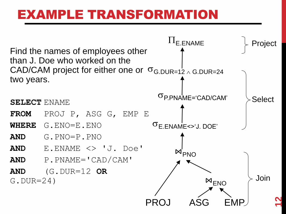
EXAMPLE TRANSFORMATION
12
Find the names of employees other than J. Doe who worked on the CAD/CAM project for either one or two years.
SELECT ENAME
FROM PROJ P, ASG G, EMP E
WHERE G.ENO=E.ENO
AND G.PNO=P.PNO
AND E.ENAME <> 'J. Doe'
AND P.PNAME='CAD/CAM'
AND (G.DUR=12 OR
G.DUR=24)
E.ENAME
G.DUR=12 G.DUR=24
P.PNAME=‘CAD/CAM’
E.ENAME<>‘J. DOE’
PROJ ASG EMP
Project
Select
Join
⋈PNO
⋈ENO

EQUIVALENT QUERY
13
E.ENAME
P.PNAME=‘CAD/CAM’ (G.DUR=12 G.DUR=24) E.ENAME<>‘J. Doe’
×
PROJ ASGEMP
⋈PNO,ENO
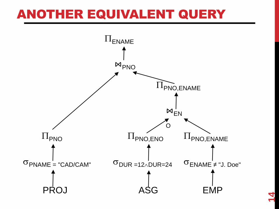
ANOTHER EQUIVALENT QUERY
14EMPASGPROJ
ENAME
ENAME ≠ "J. Doe"
PNO,ENAME
PNAME = "CAD/CAM"
PNO
DUR =12DUR=24
PNO,ENO
PNO,ENAME
⋈PNO
⋈EN
O

CLICKER QUESTION #36
Is the right query plan equivalent to the left query plan?
15
E.ENAME
G.DUR=12 G.DUR=24
P.PNAME=‘CAD/CAM’
E.ENAME<>‘J. DOE’
PROJ ASG EMP
⋈PNO
⋈EN
O
PROJ ASG EMP
P.PNAME=‘CAD/CAM’ E.ENAME<>‘J. DOE’G.DUR=12 G.DUR=24
⋈PNO
⋈EN
O
E.ENAME
(a) Yes
(b) No

IMPORTANT PROBLEM – JOIN ORDER
Assume you have
R ⋈S ⋈ T ⋈W
16
Linear Join Tree Bushy Join Tree
SR TTSR
T
W
⋈
⋈
⋈
⋈
⋈ ⋈
Most systems implement linear join trees
• Left-linear

JOIN ORDERING
Even with left-linear, how do you know which order?
• Assume natural join over common attributes
17
SR
T
W
⋈
⋈
⋈
SR
W
T
⋈
⋈
⋈
SR
W
T
⋈
⋈
⋈ …
Even with left-linear, how do you know which order?
• Assume natural join over common attributes

SOME OPERATOR IMPLEMENTATIONS
Tuple Selection
• without an index
• with a clustered index
• with an unclustered index
• with multiple indices
Projection
Joining
• nested loop join
• sort-merge join
• and others...
Grouping and Duplicate Elimination
• by sorting
• by hashing
Sorting
18

EXAMPLE – JOIN ALGORITHMS
SELECT C.Cnum, A.Balance
FROM Customer C, Accounts A
WHERE C.Cnum = A.Cnum
Nested loop join:
for each tuple c in Customer do
for each tuple a in Accounts do
if c.Cnum = a.Cnum then
output c.Cnum,a.Balance
end
end
19

EXAMPLE – JOIN ALGORITHMS (2)
SELECT C.Cnum, A.Balance
FROM Customer C, Accounts A
WHERE C.Cnum = A.Cnum
Index join:
for each tuple c in Customer douse the index to find Accounts tuples a
where a.Cnum matches c.Cnumif there are any such tuples a then
output c.Cnum, a.Balanceend
end
Sort-merge join:
sort Customer and Accounts on Cnummerge the resulting sorted relations
20

COMPLEXITY OF OPERATORS
Assume
• Relations of cardinality n
• Sequential scan
21
Operation Complexity
SelectProject
(without duplicate elimination)O(n)
Project(with duplicate elimination)
GroupO(n log n)
Join
Semi-join
Division
Set Operators
O(n log n)
Cartesian Product O(n2)
COST OF PLANS
Alternative access plans may be compared according to cost.
The cost of an access plan is the sum of the costs of its component
operations.
There are many possible cost metrics. However, most metrics
reflect the amounts of system resources consumed by the access
plan. System resources may include:
• disk block I/O’s
• processing time
• network bandwidth
22

LECTURE SUMMARY
Query processing methodology
Basic query operations and their costs
Generation of execution plans
23