Query and JoinOptimization

11/5

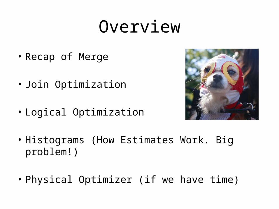
Overview

• Recap of Merge

• Join Optimization

• Logical Optimization

• Histograms (How Estimates Work. Big problem!)

• Physical Optimizer (if we have time)

Recap on Merge

Key (Simple) Idea

To find an element that is no larger than all elements in two lists, one only needs to

compare minimum elements from each list.

A1 <= A2 <= … <= AN

B1 <= B2 <= … <= BM Then Min {A1, B1} <= Ai for i=1….N and Min {A1, B1} <= Bj for j=1….M

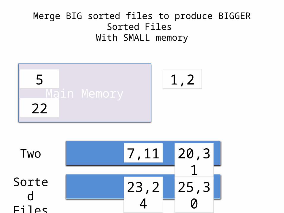
Merge BIG sorted files to produce BIGGER Sorted Files With SMALL memory

7,111, 5 20,31

2, 22 25,3023,24

Main Memory

Two Sorted

Files(disk)

Merge BIG sorted files to produce BIGGER Sorted Files With SMALL memory

7,11 20,31

25,3023,24

Main Memory

Two Sorted

Files(disk)

1, 5

2, 22

Merge BIG sorted files to produce BIGGER Sorted Files With SMALL memory

7,11 20,31

25,3023,24

Main Memory

Two Sorted

Files(disk)

1,5

2,22

Merge BIG sorted files to produce BIGGER Sorted Files With SMALL memory

7,11 20,31

25,3023,24

Main Memory

Two Sorted

Files(disk)

5

22

1,2

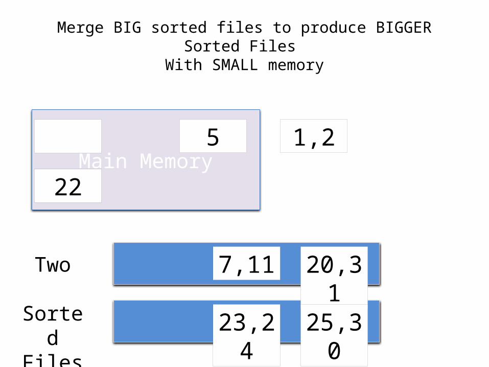
Merge BIG sorted files to produce BIGGER Sorted Files With SMALL memory

7,11 20,31

25,3023,24

Main Memory

Two Sorted

Files(disk)

5

22

1,2

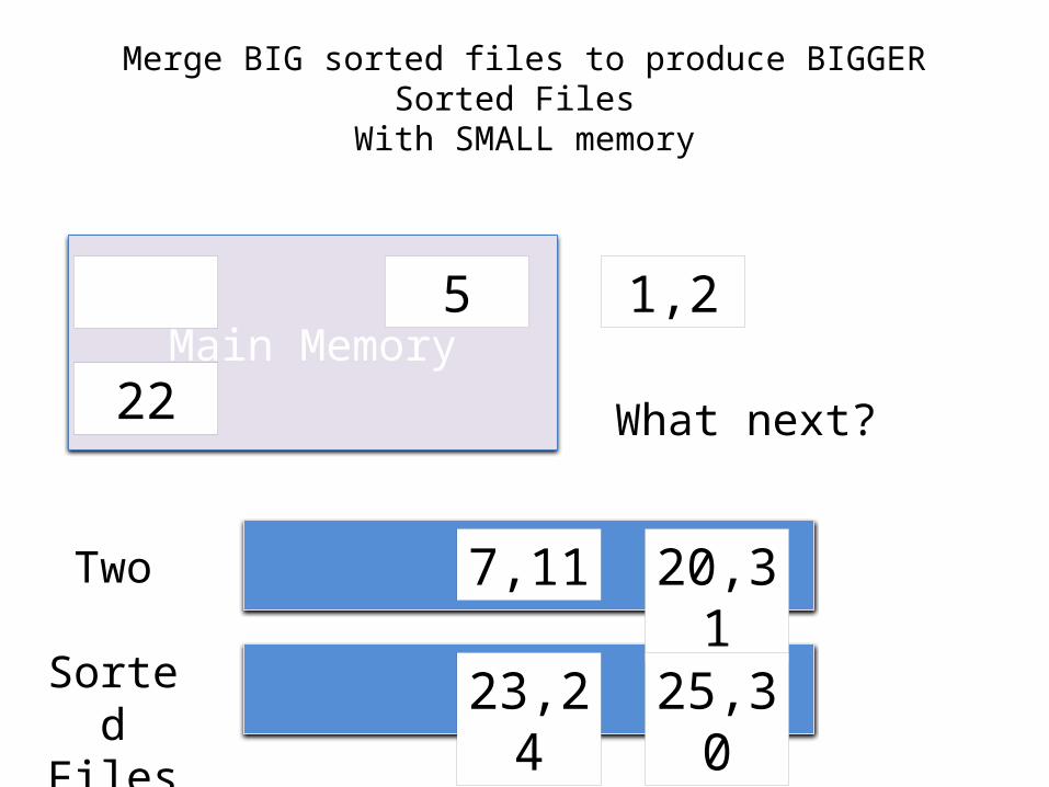
Merge BIG sorted files to produce BIGGER Sorted Files With SMALL memory

7,11 20,31

25,3023,24

Main Memory

Two Sorted

Files(disk)

22

1,25

What next?

Merge BIG sorted files to produce BIGGER Sorted Files With SMALL memory

20,31

25,3023,24

Main Memory

Two Sorted

Files(disk)

22

1,25

7,11

Merge BIG sorted files to produce BIGGER Sorted Files With SMALL memory

20,31

25,3023,24

Main Memory

Two Sorted

Files(disk)

7,11

22

1,25

Merge BIG sorted files to produce BIGGER Sorted Files With SMALL memory

20,31

25,3023,24

Main Memory

Two Sorted

Files(disk)

11

22

1,25,7

Merge BIG sorted files to produce BIGGER Sorted Files With SMALL memory

20,31

25,3023,24

Main Memory

Two Sorted

Files(disk)

11

22

1,2 5,7

Merge BIG sorted files to produce BIGGER Sorted Files With SMALL memory

20,31

25,3023,24

Main Memory

Two Sorted

Files(disk)

22

1,211 5,7

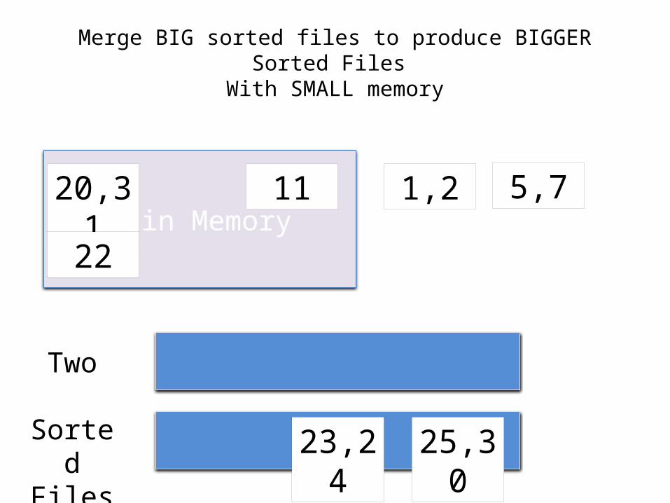
Merge BIG sorted files to produce BIGGER Sorted Files With SMALL memory

25,3023,24

Main Memory

Two Sorted

Files(disk)

20,31

22

1,211 5,7

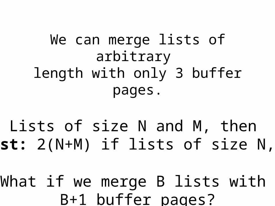
We can merge lists of arbitrary length with only 3 buffer pages.

If Lists of size N and M, thenCost: 2(N+M) if lists of size N,M.

What if we merge B lists with B+1 buffer pages?

Query Optimization

Optimization

Order the operations within a query to reduce the cost.

Major component of the database – Most mysterious & important– Heart of Query Processing (QP)

“QP is not rocket science. When you flunk out of QP, we make you go build rockets.” – anonymous

Join Optimization

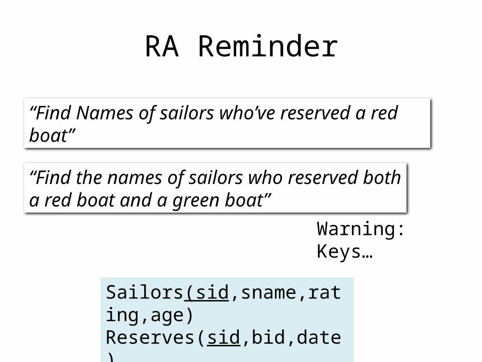
RA Reminder

Sailors(sid,sname,rating,age)Reserves(sid,bid,date)Boats(bid,bname,color)

Warning: Keys…

“Find Names of sailors who’ve reserved a red boat”

“Find the names of sailors who reserved both a red boat and a green boat”

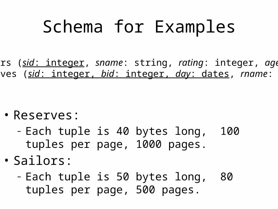
Schema for Examples

• Reserves:– Each tuple is 40 bytes long, 100 tuples per page, 1000

pages.• Sailors:

– Each tuple is 50 bytes long, 80 tuples per page, 500 pages.

Sailors (sid: integer, sname: string, rating: integer, age: real)Reserves (sid: integer, bid: integer, day: dates, rname: string)

What is this doing?

You too can type EXPLAIN!(you may also want to know ANALYZE)

When it’s slow, you’d like to know!

Joins

• One of the most important for performance

• Many, many algorithms: All fun.

SELECT * FROM Reserves R1, Sailors S1WHERE R1.sid = S1.sid

What is this in RA?

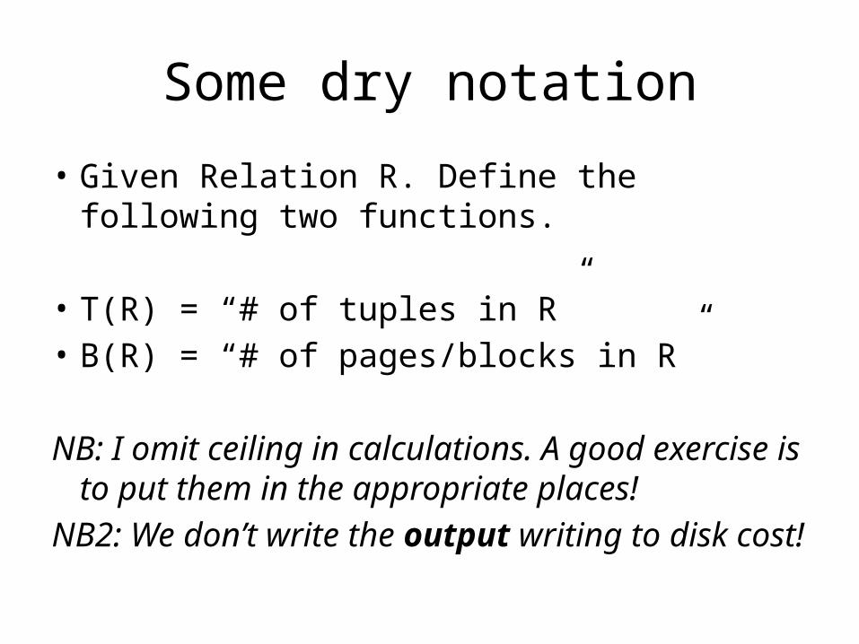
Some dry notation

• Given Relation R. Define the following two functions.

• T(R) = “# of tuples in R”• B(R) = “# of pages/blocks in R”

NB: I omit ceiling in calculations. A good exercise is to put them in the appropriate places!

NB2: We don’t write the output writing to disk cost!

26

Nested loop join

27

Nested Loop Joins

• Tuple-based nested loop R S

for each tuple r in R do for each tuple s in S do if r and s join then output (r,s)

B(R) = 500 T(R) = 50,000B(S) = 1000 T(S) =200,000then, 5e7 IOs. ~ 140 hours!

Cost: B(R) + T(R) B(S). Why?

What is the cost if we switch the R and S?

28

Block Nested Loop Joins

for each (M-1) blocks br of R do for each block bs of S do for each tuple s in bs do for each tuple r in br do if r and s join then output(r,s)

Let M be the number of blocks

in memory (M=11)

B(R) = 500 T(R) = 50,000B(S) = 1000 T(S) =200,000NLJ =140 hrs BNLJ=.14 hrs

NLJ = B(R) + T(R)B(S)BNLJ = B(R) + B(R)B(S)/(M-1)

29

Nested Loop Joins• Block-based Nested Loop Join– Still a smart cross product. Nevertheless,

useful!

• NB: it is faster to iterate over the smaller relation first

• R S: R=outer relation, S=inner relation

Smarter than Cross Products

31

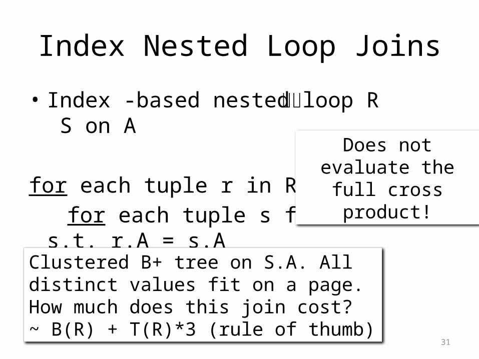
Index Nested Loop Joins

• Index -based nested loop R S on A

for each tuple r in R do for each tuple s find all s.t. r.A = s.A

Clustered B+ tree on S.A. All distinct values fit on a page. How much does this join cost?~ B(R) + T(R)*3 (rule of thumb)

Does not evaluate the full cross product!

Sort Merge

Join: Sort-Merge (R S)

• Sort R and S on the join column, then scan them to do a ``merge’’ (on join col.), and output result tuples.

• R is scanned once; each S group is scanned once per matching R tuple. – Multiple scans of an S group are likely to find needed

pages in buffer.

If R, S are already sorted on the join key, SMJ is awesome!

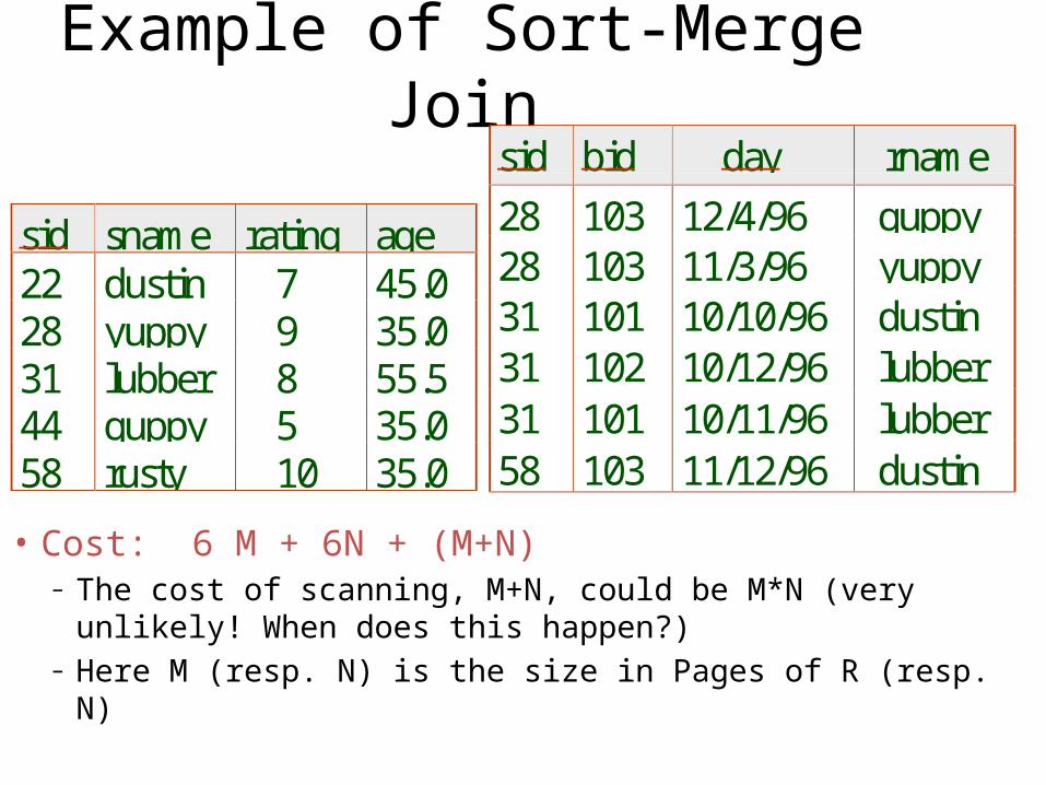
Example of Sort-Merge Join

• Cost: 6 M + 6N + (M+N)– The cost of scanning, M+N, could be M*N (very unlikely!

When does this happen?)– Here M (resp. N) is the size in Pages of R (resp. N)

sid sname rating age22 dustin 7 45.028 yuppy 9 35.031 lubber 8 55.544 guppy 5 35.058 rusty 10 35.0

sid bid day rname

28 103 12/4/96 guppy28 103 11/3/96 yuppy31 101 10/10/96 dustin31 102 10/12/96 lubber31 101 10/11/96 lubber58 103 11/12/96 dustin

Sort Merge v. Nested Loops steel cage match

• If we have 100 buffer pages, reserves is 1000 pages and Sailors 500 pages then– Sort both in two passes: 2 * 2 * 1000 + 2 * 2 * 500– Merge phase 1000 + 500 so 7500 IOs

• What is BNLJ?– 500 + 1000*500/99 = 5550

• But, if we have 35 buffer pages?– Sort Merge has same behavior (still 2 pass)– BNLJ? ~ 15k IOs!

NB: SMJ both relations sorted in two passes

A simple optimization: Merged!

Observe. The last phase of the external sort is a merge, and we can merge the merge phases.– Create sorted runs 2 * (1000 + 500)• Each run is of length (B-1) (approximately)• There are 1000/(B-1) + 500/(B-1) such runs

– If (1000+500)/(2(B-1)) < B-1 then all runs fit in memory, roughly if (M+N) < 2B2 or max { M, N } < 2B2

– One can create runs of length 2(B-1) using what’s called a tournament sort used in PostgreSQLSo we’ll say max { M, N } < B2

implies cost 3(M+N)

Hash Join

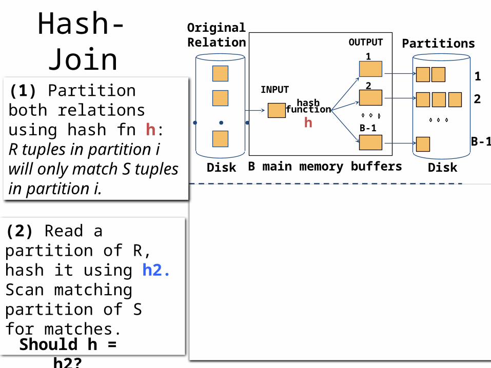
Hash-Join

Partitionsof R & S

Input bufferfor Si

Hash table for partitionRi (k < B-1 pages)

B main memory buffersDisk

Output buffer

Disk

Join Result

hashfnh2

h2

B main memory buffers DiskDisk

Original Relation OUTPUT

2INPUT

1

hashfunction

h B-1

Partitions

1

2

B-1

. . .

(2) Read a partition of R, hash it using h2.Scan matching partition of S for matches.

(1) Partition both relations using hash fn h: R tuples in partition i will only match S tuples in partition i.

Should h = h2?

How much memory does Hash join need to perform well?

Good case=perform the join in 2 passes1st Point: How large are the partitions?– R is of size M – S is of size N (wlog M < N)– Partition R into B-1 buffer pages (why B-1?)• How many partitions result? How big are they?

Roughly, each partition of R is f M/(B-1)where f is some fudge factor.

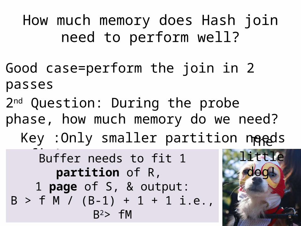
How much memory does Hash join need to perform well?

Good case=perform the join in 2 passes2nd Question: During the probe phase, how much memory do we need?

Key :Only smaller partition needs to fit!

Buffer needs to fit 1 partition of R, 1 page of S, & output:

B > f M / (B-1) + 1 + 1 i.e., B2> fM

The little dog!

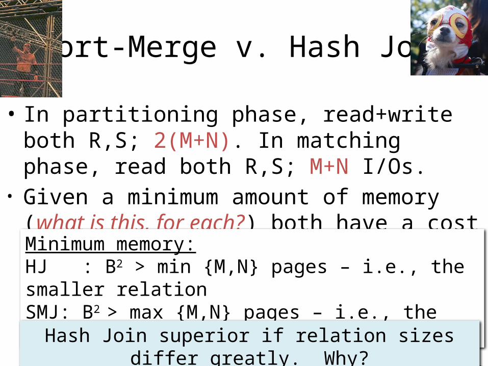
Sort-Merge v. Hash Join

• In partitioning phase, read+write both R,S; 2(M+N). In matching phase, read both R,S; M+N I/Os.

• Given a minimum amount of memory (what is this, for each?) both have a cost of 3(M+N) I/Os.

Minimum memory:HJ : B2 > min {M,N} pages – i.e., the smaller relationSMJ: B2 > max {M,N} pages – i.e., the larger relation.

Hash Join superior if relation sizes differ greatly. Why?

Further Comparisons of Hash and Sort Joins

• Hash Joins are highly parallelizable.

• Sort-Merge less sensitive to data skew and result is sorted

Observations about Hash-Join

• In-memory hash table speeds up matching tuples, so little more memory is needed (fudge factor).

• If the hash function does not partition uniformly, one or more R partitions may not fit in memory.– What then? Can apply hash-join technique recursively

to do the join of this R-partition with corresponding S-partition.

– SKEW!

Recall: Logical Optimization

Single block SQL to RA

SELECT DISTINCT S.sidFROM Sailors S, Reserves RWHERE s.sid = r.sid and s.rating > 8

SELECT S.sid, COUNT(DISTINCT Bid)FROM Sailors S, Reserves RWHERE s.sid = r.sid and s.rating > 8GROUP BY S.sidHAVING COUNT(DISTINCT Bid) > 5

Highly rated sailors who reserve many different boats and how many boats they reserve

How would you optimize

these?

Highly rated sailors

Logical Optimization Summary

Use query equivalence to compute same output via different plans– Key reason to use an algebra

Often logical rewritings applied heuristically:– Always convert selection + cross product to Join• Asymptotic reduction

– Push down selections and projections• Often, but not always a good idea!

Physical Optimization

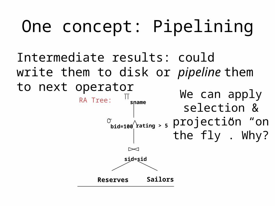
One concept: Pipelining

Intermediate results: could write them to disk or pipeline them to next operator

Reserves Sailors

sid=sid

bid=100 rating > 5

snameRA Tree:We can apply

selection & projection “on the fly”. Why?

Overview of Query Optimization

A Plan is Tree of R.A. ops with choice of algorithm for each op.

– Each operator typically implemented using a `pull’ interface:

Two main issues:– For a given query, what plans are considered?

• Algorithm to search plan space for cheapest (estimated) plan.– How is the cost of a plan estimated?

Ideally: Want to find best plan. Practically: Avoid worst plans!We will study the System R approach.

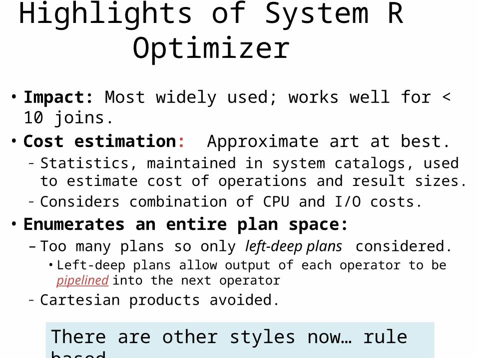
Highlights of System R Optimizer

• Impact: Most widely used; works well for < 10 joins.• Cost estimation: Approximate art at best.

– Statistics, maintained in system catalogs, used to estimate cost of operations and result sizes.

– Considers combination of CPU and I/O costs.• Enumerates an entire plan space: – Too many plans so only left-deep plans considered.

• Left-deep plans allow output of each operator to be pipelined into the next operator

– Cartesian products avoided.

There are other styles now… rule based.

An Example

How does it get those costs?

Cost Estimation

Cost Estimation

For each plan considered, must estimate cost:– Must estimate cost of each operation in plan tree.• You know or can guess this: We’ve already discussed

how to estimate the cost of operations (sequential scan, index scan, joins, etc.)• All estimates depend on input cardinality…

– Must also estimate size of result for each operation in tree!• For selections and joins, assume independence of

predicates.

Let’s see how to estimate…

Histograms

Histograms

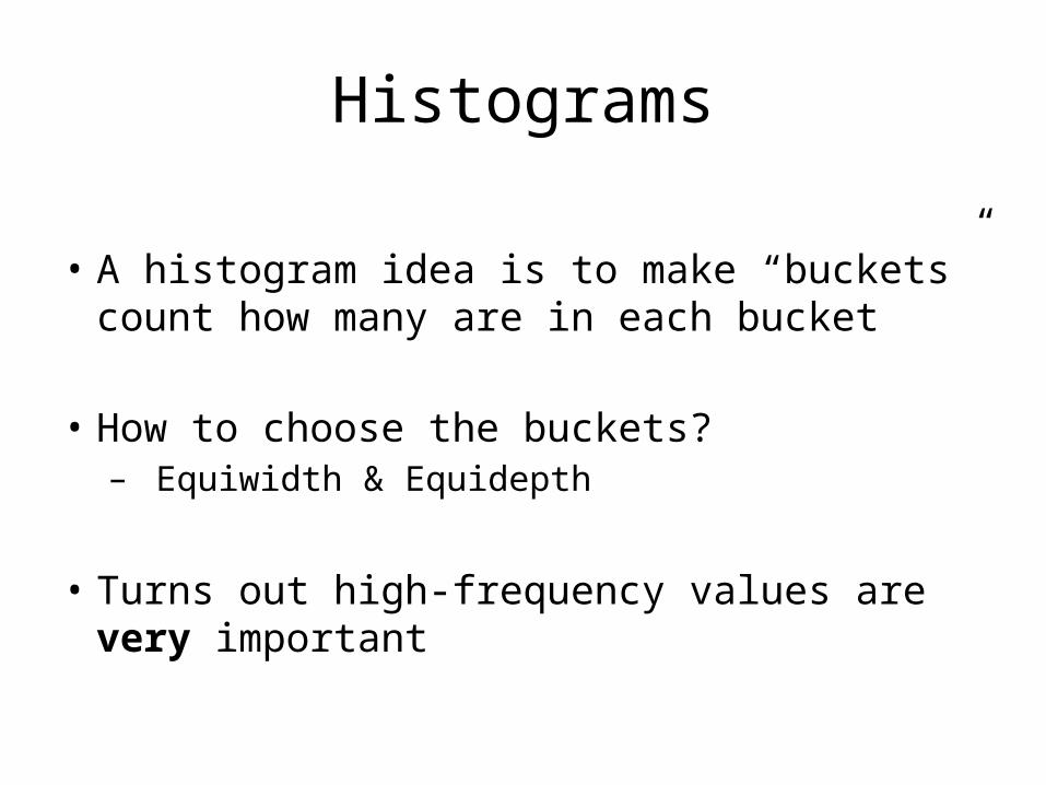
• A histogram idea is to make “buckets” count how many are in each bucket

• How to choose the buckets?– Equiwidth & Equidepth

• Turns out high-frequency values are very important

Abstract Example

1 2 3 4 5 6 7 8 9 10 11 12 13 14 150

2

4

6

8

10

Values

Frequency

How do we compute how many values between 8 and 10?

(Yes, it’s obvious)

Problem: Counts take too much

space!

The Uniform is Red

1 2 3 4 5 6 7 8 9 10 11 12 13 14 150123456789

10

How much space does this take to store?

Fundamental Tradeoffs

• Want high resolution (like the full counts)

• Want low space (like uniform)

• Histograms are a compromise!

The Uniform is Red

1 2 3 4 5 6 7 8 9 10 11 12 13 14 150123456789

10

A query

How do you estimate # of tuples? What about point queries?

Equi width

1 2 3 4 5 6 7 8 9 10 11 12 13 14 150123456789

10

All buckets roughly the same width

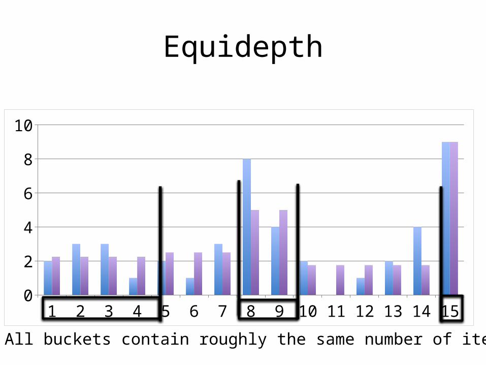
Equidepth

1 2 3 4 5 6 7 8 9 10 11 12 13 14 150123456789

10

All buckets contain roughly the same number of items

Range Query: x in [5,8]

1 2 3 4 5 6 7 8 9 10 11 12 13 14 150123456789

10

All buckets roughly the same width

Histograms

• Simple, intuitive and popular

• Parameters # of buckets and type

• Can extend to many attributes (multidimensional)

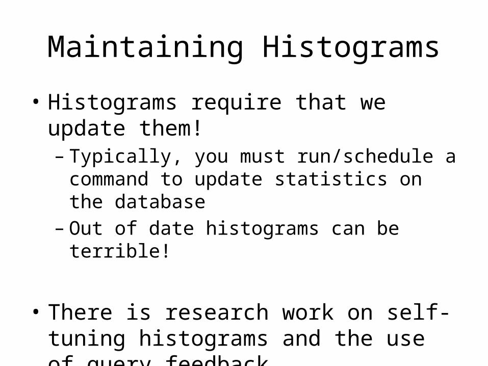
Maintaining Histograms

• Histograms require that we update them!– Typically, you must run/schedule a command to

update statistics on the database– Out of date histograms can be terrible!

• There is research work on self-tuning histograms and the use of query feedback– Oracle 11g

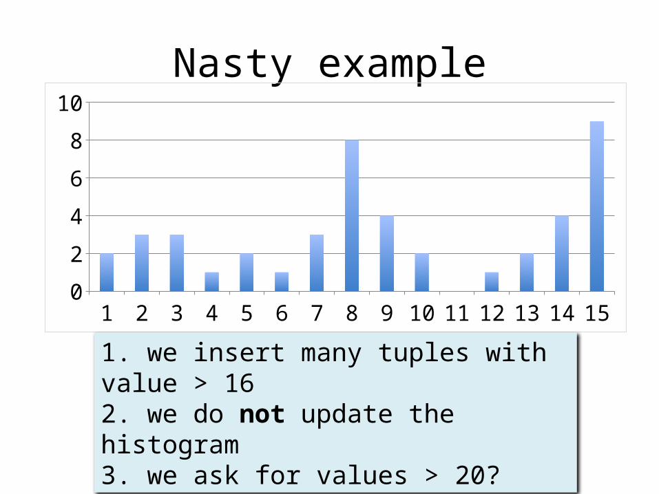
Nasty example

1 2 3 4 5 6 7 8 9 10 11 12 13 14 150

2

4

6

8

10

1. we insert many tuples with value > 162. we do not update the histogram3. we ask for values > 20?

When estimates behave badly

• If we underestimate the number of tuples, what kinds of plans suffer?

• If we overestimate the number of tuples, what kinds of plans suffer?

Think about using unclustered indexes….

We could have used that index! Or we could have used a hash join in one pass instead of sorting in two!

Compressed Histograms

• One popular approach: 1. Store the most frequent values and their counts

explicitly2. Keep an equiwidth or equidepth one for the rest

of the values

People continue to try all manner of fanciness here that people try wavelets,

graphical models, entropy models,…