Quaternions—An Algebraic View (Supplement)bra. John Fraleigh’s A First Course in Abstract...

Quaternions—Algebraic View (Supplement) 1

Quaternions—An Algebraic View (Supplement)

Note. You likely first encounter the quaternions in Introduction to Modern Alge-

bra. John Fraleigh’s A First Course in Abstract Algebra, 7th edition (Addison Wes-

ley, 2003), defines the quaternions in Part IV (Rings and Fields), Section 24 (Non-

commutative Examples—see pages 224 and 225). However, this is an “optional”

section for Introduction to Modern Algebra 1 (MATH 4127/5127). In Modern Alge-

bra 1 (MATH 5410) Thomas Hungerford’s Algebra (Springer-Verlag, 1974) defines

them in his Chapter III (Rings), Section III.1 (Rings and Homomorphisms—see

page 117). We now initially follow definitions of Hungerford.

Definition (Hungerford’s III.1.1). A ring is a nonempty set R together with

two binary operations (denoted + and multiplication) such that:

(i) (R,+) is an abelian group.

(ii) (ab)c = a(bc) for all a, b, c ∈ R (i.e., multiplication is associative).

(iii) a(b + c) = ab + ac and (a + b)c = ac + bc (left and right distribution of

multiplication over +).

If in addition,

(iv) ab = ba for all a, b ∈ R,

then R is a commutative ring. If R contains an element 1R such that

(v) 1Ra = a1R = a for all a ∈ R,

then R is a ring with identity (or unity).


Note. An obvious “shortcoming” of rings is the possible absence of inverses under

multiplication. We adopt the standard notation from (R,+). We denote the +

identity as 0 and for n ∈ Z and a ∈ R, na denotes the obvious repeated addition.

Definition (Hungerford’s III.1.3). A nonzero element a in the ring R is a left

(respectively, right) zero divisor if there exists a nonzero b ∈ R such that ab = 0

(respectively, ba = 0). A zero divisor is an element of R which is both a left and

right zero divisor.

Definition (Hungerford’s page 117). Let S = {1, i, j, k}. Let H be the ad-

ditive abelian group R ⊕ R ⊕ R ⊕ R and write the elements of H as formal sums

(a0, a1, a2, a3) = a01 + a1i + a2j + a3k. We often drop the “1” in “a01” and replace

it with just a0. Addition in H is as expected:

(a0+a1i+a2j+a3k)+(b0+b1i+b2j+b3k) = (a0+b0)+(a1+b1)i+(a2+b2)j+(a3+b3)k.

We turn H into a ring by defining multiplication as

(a0 + a1i + a2j + a3k)(b0 + b1i + b2j + b3k) = (a0b0 − a1b1 − a2b2 − a3b3)

+(a0b1+a1b0+a2b3−a3b2)i+(a0b2+a2b0+a3b1−a1b3)j+(a0b3+a3b0+a1b2−a2b1)k.

This product can be interpreted by considering:

(i) multiplication in the formal sum is associative,

(ii) ri = ir, rj = jr, rk = kr for all r ∈ R,

(iii) i2 = j2 = k2 = ijk = −1, ij = −ji = k, jk = −kj = i, ki = −ik = j.

This ring is called the real quaternions and is denoted H in commemoration of Sir

William Rowan Hamilton (1805–1865) who discovered them in 1843.


Definition (Hungerford’s III.1.5). A commutative ring R with (multiplicative)

identity 1R and no zero divisors is an integral domain. A ring D with identity 1D 6= 0

in which every nonzero element is a unit is a division ring. A field is a commutative

division ring.

Note. First, it is straightforward to show that 1 = (1, 0, 0, 0) is the identity in

H. However, since ij = −ji 6= ji, then H is not commutative and so H is not an

integral domain nor a field.

Theorem. The quaternions form a noncommutative division ring.

Proof. Tedious computations confirm that multiplication is associative and the

distribution law holds. We now show that every nonzero element of H has a multi-

plicative inverse. Consider q = a0+a1i+a2j+a3k. Define d = a20+a2

1+a22+a2

3 6= 0.

Notice that

(a0 + a1i + a2j + a3k)((a0/d) − (a1/d)i − (a2/d)j − (a3/d)k)

= (a0(a0/d) − a1(−a1/d) − a2(−a2/d) − a3(−a3/d))

+(a0(−a1/d) + a1(a0/d) + a2(−a3/d) − a3(−a2/d))i

+(a0(−a2/d) + a2(a0/d) + a3(−a1/d) − a1(−a3/d))j

+(a0(−a3/d) + a3(a0/d) + a1(−a2/d) − a2(−a1/d))k

= (a20 + a2

1 + a22 + a2

3)/d = 1.

So (a0 + a1i + a2j + a3k)−1 = (a0/d) − (a1/d)i − (a2/d)j − (a3/d)k where d =

a20 + a2

1 + a22 + a2

3. Therefore every nonzero element of H is a unit and so the

quaternions form a noncommutative division ring.


Note. Since every nonzero element of H is a unit, the H contains no left zero

divisors: If q1q2 = 0 and q1 6= 0, then q2 = q−11 0 = 0. Similarly, H has no right zero

divisors.

Note. I use the 8-element multiplicative group {±1,±i,±j,±k} (called by Hunger-

ford the “quaternion group”; see his Exercise I.2.3) to illustrate Cayley digraphs of

groups in my Introduction to Modern Algebra (MATH 4127/5127) notes:

http://faculty.etsu.edu/gardnerr/4127/notes/I-7.pdf).

Consider the Cayley digraph given below. This is the Cayley digraph for a multi-

plicative group of order 8, denoted Q8. The dotted arrow represents multiplication

on the right by i and the solid arrow represents multiplication on the right by j.

The problem is to use this diagram to create a multiplication table for Q8.


Solution. For multiplication on the right by i we have: 1 · i = i, i · i = −1,

−1 · i = −i, −i · i = 1, j · i = −k, −k · i = −j, −j · i = k, and k · i = j. For

multiplication on the right by j we have: 1 · j = j, j · j = −1, −1 · j = −j,

−j · j = 1, i · j = k, k · j = −i, −i · j = −k, and −k · j = i. This gives us 16

of the entries in the multiplication table for Q8. Since 1 is the identity, we get

another 15 entries. All entries can be found from this information. For example,

k · k = k · (i · j) = (k · i) · j = (j) · j = −1. The multiplication table is:

· 1 i j k −1 −i −j −k

1 1 i j k −1 −i −j −k

i i −1 k −j −i 1 −k j

j j −k −1 i −j k 1 −i

k k j −i −1 −k −j i 1

−1 −1 −i −j −k 1 i j k

−i −i 1 −k j i −1 k −j

−j −j k 1 −i j −k −1 i

−k −k −j i 1 k j −i −1

This group is addressed in Hungerford in Exercises I.2.3, I.4.14, and III.1.9(a).

Notice that each of i, j, and k are square roots of −1. So the quaternions are, in

a sense, a generalization of the complex numbers C. The Galois group AutQQ(α),

where α =√

(2 +√

2)(3 +√

3), is isomorphic to Q8 (see page 584 of D. Dummit

and R. Foote’s Abstract Algebra, 3rd edition, John Wiley and Sons (2004)).


Note. The quaternions may also be interpreted as a subring of the ring of all 2×2

matrices over C. This is Exercise III.1.8 of Hungerford (see page 120): “Let R be

the set of all 2×2 matrices over the complex field C of the form

z w

−w z

, where

z, w are the complex conjugates of a and w, respectively. Prove that R is a division

ring and that R is isomorphic to the division ring of real quaternions.” In fact,

the quaternion group, Q8, can be thought of as the group of order 8 generated by

A =

0 1

−1 0

and B =

0 i

i 0

, under matrix multiplication (see Hungerford’s

Exercise I.2.3).

Note. In fact, the complex numbers can be similarly represented as the field of

all 2 × 2 matrices of the form

a −b

b a

where a, b ∈ R (see Exercise I.3.33 of

Fraleigh).

Note. The complex numbers can be defined as ordered pairs of real numbers,

C = {(a, b) | a, b ∈ R}, with addition defined as (a, b) = (c, d) = (a + c, b + d)

and multiplication defined as (a, b)(c, d) = (ac − bd, bc + ad). We then have that

C is a field with additive identity (0, 0) and multiplicative identity (1, 0). The

additive inverse of (a, b) is (−a,−b) and the multiplicative inverse of (a, b) 6=(0, 0) is (a/(a2 + b2),−b/(a2 + b2)). We commonly denote (a, b) as “a + ib” so

that i = (0, 1) and we notice that i2 = −1. In fact, this is the definition of

the complex field in our graduate level Complex Analysis 1 (MATH 5510); see

http://faculty.etsu.edu/gardnerr/5510/notes/I-2.pdf for the notes from this


class in which C is so defined. The complex numbers are visualized as the “com-

plex plane” where a + ib ∈ C is associated with (a, b) ∈ R2. During the early

decades of the 19th century, the complex numbers became an accepted part of

mathematics (in large part due to the development of complex function theory by

Augustin Cauchy). Since the complex numbers have an interpretation as a sort of

“two dimensional” number system, a natural question to ask is: “Is there a three

(or higher) dimensional number system?”

Note. Sir William Rowan Hamilton (1805–1865) spent the years 1835 to 1843

trying to develop a three dimensional number system based on triples of real num-

bers. He never succeeded. However, he did succeed in developing a four dimensional

number system, now called the quaternions and denoted “H” in his honor. In a

letter he wrote late in his life to his son Archibald Henry, Hamilton tells the story

of his discovery:

“Every morning in the early part of [October 1843], on my coming down

to breakfast, your little brother, William Edwin, and yourself, used to

ask me, ‘Well, papa, can you multiply triplets?’ Whereto I was always

obliged to reply, with a sad shake of the head: ‘No, I can only add and

subtract them.’ But on the 16th day of that some month. . . An electric

circuit seemed to close; and a spark flashed forth the herald (as I foresaw

immediately) of many long years to come of definitely directed through

and work by myself, is spared, and, at all events, on the part of others if

I should even be allowed to live long enough distinctly to communicate

the discovery. Nor could I resist the impulse—unphilosophical as it


may have been—to cut with a knife on a stone of Brougham Bridge

[in Dublin, Ireland; now called “Broom Bridge”], as we passed it, the

fundamental formula with the symbols i, j, k:

i2 = j2 = k2 = ijk = −1

which contains the Solution of the Problem, but, of course, the inscrip-

tion has long wince mouldered away.”

So the exact date of the birth of the quaternions is October 16, 1843. [This note

is based on Unknown Quantity: A Real and Imaginary History of Algebra by John

Derbyshire, John Henry Press (2006).]

William Rowan Hamilton Plaque on the Broom Bridge

Images from http://www-groups.dcs.st-and.ac.uk/ history/Biographies/Hamilton.html

and http://motls.blogspot.com/2015/08/william-rowan-hamilton-210th-birthday.html

Note. You are probably familiar with the Factor Theorem which relates roots of a

polynomial to linear factor of the polynomial. You might not recall that it requires

commutivity, though:


The Factor Theorem. (Hungerford’s Theorem III.6.6). Let R be a com-

mutative ring with identity and f ∈ R[x]. Then c ∈ R is a root of f if and only if

x − c divides f .

Note. The Factor Theorem is used to prove the following, which might remind

you of the Fundamental Theorem of Algebra:

Hungerford’s Theorem III.6.7. If D is an integral domain contained in an

integral domain E and f ∈ D[x] has degree n, then f has at most n distinct roots

in E.

So in an integral domain, an n degree polynomial at most n roots. Surprisingly in

a division ring, this can be violated.

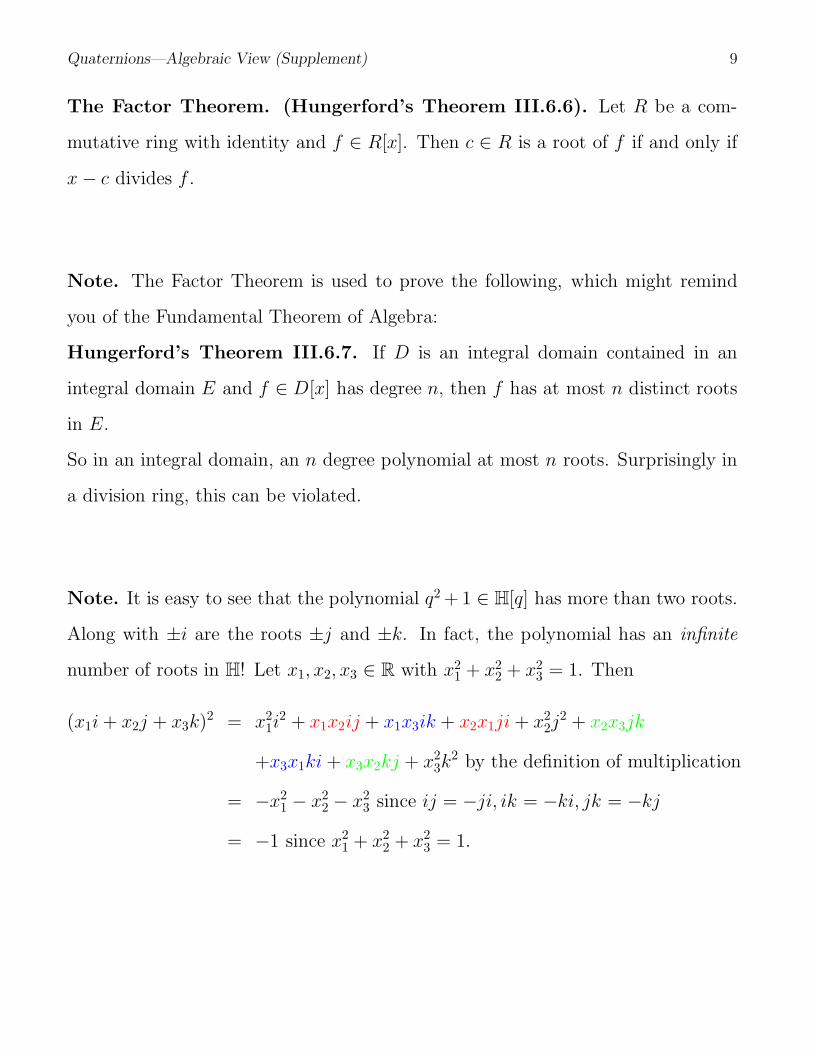
Note. It is easy to see that the polynomial q2 + 1 ∈ H[q] has more than two roots.

Along with ±i are the roots ±j and ±k. In fact, the polynomial has an infinite

number of roots in H! Let x1, x2, x3 ∈ R with x21 + x2

2 + x23 = 1. Then

(x1i + x2j + x3k)2 = x21i

2 + x1x2ij + x1x3ik + x2x1ji + x22j

2 + x2x3jk

+x3x1ki + x3x2kj + x23k

2 by the definition of multiplication

= −x21 − x2

2 − x23 since ij = −ji, ik = −ki, jk = −kj

= −1 since x21 + x2

2 + x23 = 1.


Note. We now turn our attention to polynomials in H[x]. We are particularly

interested in roots of such polynomials, a version of the Factor Theorem, and the

concept of algebraic closure. Much of this material is of fairly recent origins. The

remainder of the supplement is mostly based on the following references:

1. T. Y. Lam, A First Course in Noncommutative Rings, Graduate Texts in Math-

ematics #131, Springer-Verlag (1991).

2. G. Gentili and D. C. Struppa, A New Theory of Regular Functions of a Quater-

nionic Variable, Advances in Mathematics 216 (2007), 279–301.

Definition. We denote by S the two dimensional sphere (as a subset of the four

dimensional quaternions H) S = {q = x1i + x2j + x3k | x21 + x2

2 + x23 = 1}. As

observed above, for any I ∈ S we have I2 = −1. For x, y ∈ R we let x + yS denote

the two dimensional sphere x + yS = {x + yI | I ∈ S}. (We might think of x + yS

as a two dimensional sphere centered at (x, 0, 0, 0) with radius |y|.)

Note. We take q as the indeterminate in the ring of polynomials H[q]. Since

H is not commutative, we are faced with the case that a monomial of the form

aqn ∈ H[q] is the same as monomial a1qa1qa2q · · · qan ∈ H[q] where a = a0a1 · · · an,

but if we evaluate aqn at some element of H, we may get a different value than

if we evaluate aqqa1q · · · qan at the same element of H. That is, evaluation of an

element of H[q] at r ∈ H is not a homomorphism (recall that Fraleigh deals with

the evaluation homomorphism for field theory in Theorem 22.4). In the remainder

of this supplement, we consider polynomials with the powers of the indeterminate

on the left and the coefficients on the right: p(q) =∑n

i=0 qiai. We will call p a

“quaternionic polynomial.”


Definition. For two quaternionic polynomials p1(q) =∑n

i=0 qiai and p2(q) =∑m

i=0 qibi in H[q], define the product

(p1p2)(q) =∑

i=0,1,...,n;j=0,1,...,m

qi+jaibj.

Note. We now explore roots of quaternionic polynomials. The following result is

originally due to A. Pogorui and M. V. Shapiro (in “On the Structure of the Set

of Zeros of Quaternionic Polynomials,” Complex Variables 49(6) (2004), 379–389)

but we present an easier proof due to Gentili and Struppa in 2007.

Theorem. Let p(q) =∑N

n=0 qnan be a given quaternionic polynomial. Suppose

that there exist x0, y0 ∈ R and I, J ∈ S with I 6= J such that p(x0 + y0I) = 0 and

p(x0 + y0J) = 0. Then for all L ∈ S we have p(x0 + y0L) = 0.

Proof. For any n ∈ N and any L ∈ S we have that (x0+y0L)n =∑n

i=0

(

n

i

)

xn−i0 yi

0Li =

αn + Lβn by the Binomial Theorem for a ring with identity (since x0y0L = Lx0y0

because x0, y0 ∈ R; see Theorem III.1.6 of Hungerford) where

αn =∑

i≡0(mod 4)

(

n

i

)

xn−i0 yi

0 −∑

i≡2(mod 4)

(

n

i

)

xn−i0 yi

0

and

βn =∑

i≡1(mod 4)

(

n

i

)

xn−i0 yi

0 −∑

i≡3(mod 4)

(

n

i

)

xn−i0 yi

0

because L0(mod 4) = 1, L1(mod 4) = L , L2(mod 4) = −1 , and L3(mod 4) = −L. We

therefore have

0 = 0 − 0 =

N∑

n=0

(αn + Iβn)an −N∑

n=0

(αn + Jβn)an


=

N∑

n=0

((αn + Iβn) − (αn + Jβn))an =

N∑

n=0

(I − J)βnan = (I − J)

N∑

n=0

βnan.

By hypothesis, I − J 6= 0 so (since H has no zero divisors)∑N

n=0 βnan = 0 and so

0 = p(x0 + y0I) =

N∑

n=0

(x0 + y0I)nan =

N∑

n=0

(αn + Iβn)an

=

N∑

n=0

αnan + I

N∑

n=0

βnan =

N∑

n=0

αnan.

Now for any L ∈ S we have that

p(x0 + y0L) =

N∑

n=0

(x0 + y0L)nan =

N∑

n=0

(αn + Lβn)an

=

N∑

n=0

αnan + L

N∑

n=0

βnan = 0 + 0 = 0.

Note. In fact, Gentili and Struppa develop a theory of analytic functions of a

quaternionic variable and show that the previous result holds for an analytic func-

tion.

Note. In a ring of polynomials, R[t], each element of R commutes with in-

determinate t (see Hungerford’s Theorem III.5.2(ii)). So in R[t] we have that

f(r) =∑n

i=0 aiti =

∑ni=0 tiai. However, for r ∈ R where R is not commutative

we likely have∑n

i=0 airi 6= ∑n

i=0 riai. So in order to evaluate f(r), we must de-

cide on a standard representation of f(t). In this supplement, we use the form

f(t) =∑n

i=0 tiai ∈ R[t]. Additionally, we may have f(t) = g(t)h(t) in R[t], but we


may not have f(r) = g(r)h(r). Consider g(t) = t−a and h(t) = t−b where a, b ∈ R

do not commute (so ab 6= ba). Then we have by the definition of multiplication

that f(t) = g(t)h(t) = (t − a)(t − b) = t2 − t(a + b) + ab. But

f(a) = a2 − a(a + b) + ab = ab − ba 6= 0 = g(a)h(a).

(This “sneaky” behavior results from the term at being expressed as ta in the

representation of g(t)h(t).)

Definition 16.1 of Lam. Let R be a ring and f(t) =∑n

i=0 tiai ∈ R[t]. An element

r ∈ R is a left root of f if f(r) =∑n

i=0 riai = 0. If g(t) =∑n

i=0 aiti ∈ R[t]. An

element r ∈ R is a right root of g if g(r) =∑n

i=0 airi = 0.

Proposition 16.2 of Lam. (The Factor Theorem in a Ring with Unity). An

element r ∈ R is a left (right) root of a nonzero polynomial f(t) =∑n

i=0 tiai ∈ R[t]

if and only if t − r is a left (right) divisor of f(t) in R[t].

Proof. We give a proof for left roots and divisors with the proof for right being

similar. First, if

f(t) =

n∑

i=0

tiai = (t − r)

n−1∑

i=0

tici =

n−1∑

i=0

ti+1ci −n−1∑

i=0

tirci

then

f(r) =

n−1∑

i=0

ri+1ci −n−1∑

i=0

ri+1ci = 0.

Second, suppose f(r) =∑n

i=0 riai = 0. By the Remainder Theorem (Hunger-

ford’s Corollary III.6.3 which is stated for x − r on the right, but the result also


holds for x − r on the left; this result holds in rings with unity) there is a unique

g(t) ∈ R[t] such that

f(t) = (t − r)g(t) + f(r) = (t − r)g(t) + 0 = (t − r)g(t).

So t − r is a left divisor of f(t).

Note. Recall a right ideal of a ring R is a subring I of R such that for all r ∈ R

and x ∈ I we have xr ∈ I (Hungerford’s Definition III.2.1). We see from the Factor

Theorem in a Ring with Unity that the set of polynomials in R[t] having r as a left

root is precisely the right ideal (t − r)R[t] = {(t − r)g(t) | g(t) ∈ R[t]}.

Proposition 16.3 of Lam. Let D be a division ring and let f(t) = h(t)g(t) in

D[t]. Let d ∈ D be such that a = h(d) 6= 0. Then f(d) = h(d)g(a−1da). In

particular, if d is a left root of f but not of h then the conjugate of d, a−1da, is a

left root of g.

Proof. Let g(t) =∑n

i=0 tibi. Then f(t) = h(t)g(t) =∑n

i=0 tih(t)bi and so

f(d) =n∑

i=0

dih(d)bi =n∑

i=0

diabi =n∑

i=0

aa−1diabi

=

m∑

i=0

a(a−1da)ibi = ag(a−1da) = h(d)g(a−1da).

If d is a left root of f but not a left root of h then, since D has no zero divisors,

a−1da must be a left root of g.

Note. A result similar to Proposition 16.3 holds for right roots.


Note. If D is an integral domain and p ∈ D[x] is of degree n, then p has at most

n roots in D (see Hungerford’s Theorem III.6.7, mentioned above). This is not the

case in a division ring as illustrated by p(q) = q2 + 1 ∈ H[q], as described above.

The following result is analogous to Hungerford’s Theorem III.6.7, but for division

rings. It does not imply at most n roots, but roots from at most n conjugacy

classes.

Note. Quaternion a is a conjugate of quaternion b (in the algebraic sense) if

a = cbc−1 for some quaternion c. Notice that if a = c1b1c−11 and a = c2b2c

−12 , then

b1 = c−11 ac1 so that b1 = c−1

1 (c2b2c−12 )c1 = (c−1

1 c2)b2(c−11 c2)

−1. So conjugation is an

equivalence relation and the conjugacy classes partition H.

Theorem 16.4 of Lam. (“Gordon-Motzkin” in Lam.) Let D be a division

ring and let f be a polynomial of degree n in D[t]. Then the left (right) roots of f

lie in at most n conjugacy classes of D. If f(t) = (t− a1)(t− a2) · · · (t− an) where

a1, a2, . . . , an ∈ D, then any left (right) root of f is conjugate to some ai.

Proof. We prove this using induction. In the base case, n = 1 and so f has exactly

one left root and so the left roots lie in n = 1 conjugacy class. Now suppose that

if a polynomial is of degree n− 1, then its left roots lie in at most n− 1 conjugacy

classes. Let f be degree n and let c be a left root of f . Then by Proposition 16.2,

f(t) = (t− c)g(t) where g is of degree n−1. Suppose d 6= c is any other left root of

f . Then by Proposition 16.3, d is a conjugate to a left root of g(t) (in particular,

(d − c)−1d(d − c) = r is a left root of g so d = (d − c)r(d − c)−1). Since by the


induction hypothesis the left roots of g lie in at most n− 1 conjugacy classes, then

this arbitrary left root of f (arbitrary except that is is not c) must lie in one of

these n− 1 conjugacy classes. Adding in the conjugacy class containing c, we have

that the left roots of f lie in at most n conjugacy classes. The result now follows

in general by induction.

The proof of the second claim follows similarly by induction. The result for right

roots is similar.

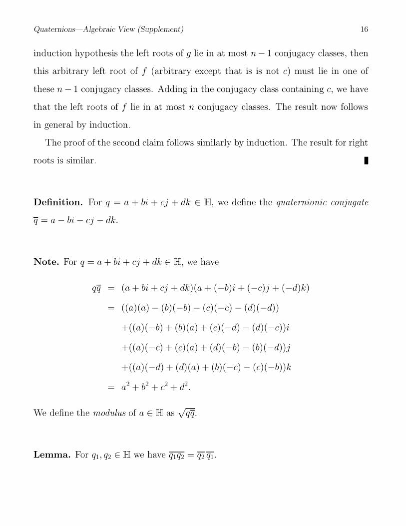
Definition. For q = a + bi + cj + dk ∈ H, we define the quaternionic conjugate

q = a − bi − cj − dk.

Note. For q = a + bi + cj + dk ∈ H, we have

qq = (a + bi + cj + dk)(a + (−b)i + (−c)j + (−d)k)

= ((a)(a)− (b)(−b)− (c)(−c) − (d)(−d))

+((a)(−b) + (b)(a) + (c)(−d) − (d)(−c))i

+((a)(−c) + (c)(a) + (d)(−b) − (b)(−d))j

+((a)(−d) + (d)(a) + (b)(−c) − (c)(−b))k

= a2 + b2 + c2 + d2.

We define the modulus of a ∈ H as√

qq.

Lemma. For q1, q2 ∈ H we have q1q2 = q2 q1.


Proof. Let q1 = a1 + b1i + c1j + d1k and q2 = a2 + b2i + c2j + d2k. Then

q1q2 = (a1 + b1i + c1j + d1k)(a2 + b2i + c2j + d2k)

= (a1a2 − b1b2 − c1c2 − d1d2) + (a1b2 + b1a2 + c1d2 − d1c2)i

+(a1c2 + c1a2 + d1b2 − b1d2)j + (a1d2 + d1a2 + b1c2 − c1b2)k

= (a1a2 − b1b2 − c1c2 − d1d2) − (a1b2 + b1a2 + c1d2 − d1c2)i

−(a1c2 + c1a2 + d1b2 − b1d2)j − (a1d2 + d1a2 + b1c2 − c1b2)k

= ((a2)(a1) − (−b2)(−b1) − (−c2)(−c1) − (−d2)(−d1))

+((−b2)(a1) + (−b1)(a2) − (−d2)(−c1) + (−c2)(−d1)i

+((−c2)(a1) + (a2)(−c1) − (−b2) − d1) + (−d2)(−b1))j

+((−d2)(a1) + (a2)(−d1) − (−c2)(−b1) + (−b2)(−c1))k

= ((a2)(a1) − (−b2)(−b1) − (−c2)(−c1) − (−d2)(−d1))

+((a2)(−b1) + (−b2)(a1) + (−c2)(−d1) − (−d2)(−c1))i

+((a2)(−c1) + (−c2)(a1) + (−d2)(−b1) − (−b2)(−d1))j

+((a2)(−d1) + (−d2)(a1) + (−b2)(−c1) − (c1)(−b1))k

= (a2 + (−b2)i + (−c2)j + (−d2)k)(a1 + (−b1)i + (−c1)j + (−d1)k)

= q2q1

Note. Recall that a field is algebraically closed if every nonconstant polynomial

over the field has a root in the field. This is the motivation for the following

definition.


Definition (Lam, page 169). A division ring D is left (right) algebraically closed

if every nonconstant polynomial in D[t] has a left (right) root in D.

Note. By Proposition 16.2, if f ∈ D[t] for left or right algebraically closed division

ring D, then f can by factored into a product of linear factors in D[t] (that is, f

splits in D[t]).

Note. The following is the Fundamental Theorem of Algebra for Quaternions.

The result originally appeared in I. Nivens’ “Equations in Quaternions,” American

Mathematical Monthly, 48 (1941), 654–661.

Theorem 16.14 of Lam. (“Niven-Jacobson” in Lam) Fundamental The-

orem of Algebra for Quaternions. The quaternions, H, are left (and right)

algebraically closed.

Proof. For f(q) =∑n

r=0 grar ∈ H[q], define f (q) =∑n

r=0 rrqar ∈ H[q]. For

f, g ∈ H[q] with f(q) =∑n

i=0 qiai and g(q) =∑m

j=0 qjbj we have

fg =

(

n∑

i=0

qiai

)(

m∑

j=0

qjbi

)

=

(

∑

i=0,1,...,n;j=0,1,...,m

qi+jaibj

)

=∑

i=0,1,...,n;j=0,1,...,m

qi+jaibj

=∑

i=0,1,...,n;j=0,1,...,m

qi+jbjai by Lemma


=

(

m∑

j=0

qjbj

)(

n∑

i=0

qiai

)

= gf.

So, in particular, ff = f f = ff , and so ff equals its own quaternionic conjugate.

Therefore the coefficients of ff must be real and ff ∈ R[q] for all f ∈ H[q].

We now use mathematical induction on n = deg(f) to prove that f has a left root

in H. For n = 1, f clearly has a left root. Suppose n ≥ 2 and that every polynomial

of degree less than n has a left root in H. Since R(i) = C ⊂ H is algebraically

closed and ff ∈ R[q] then ff has a root α in R(i) = C. By Proposition 16.3,

either α is a left root or f or a conjugate β of α is a left root of f . In the former

case we are done. In the latter case, if f(q) =∑n

r=0 qrar then f(q) =∑n

n=0 qrar

and so f(β) =∑n

r=0 βrar = 0 or∑n

r=0 arβr

= 0. That is, β is a right root of

f(q). By Theorem 16.2 (applied to a right roots) we can write f(q) = (q − β)g(q)

where g(q) ∈ H has degree n− 1. By the induction hypothesis, g(q) has a left root

γ ∈ H. But then γ is also a left root of f(q) and the general result now follows by

induction. The result for right algebraic closure is similar.

Note. Now that we have our Fundamental Theorem of Algebra, we conclude with

a brief exploration of the structure of the set of quaternions for which a polynomial

has a left (right) root. The following result is from A. Pogorui and M. Shapiro’s “On

the Structure of the Set of Zeros of Quaternionic Polynomials,” Complex Variables:

Theory and Applications 49(6) (2004), 379–389.


Theorem (Pogorui and Shapiro). For f a (nonzero) polynomial in H[q]. The

set of left (right) roots of f consists of isolated points or isolated two dimensional

spheres of the form S = x + yS for x, y ∈ R. The number of isolated roots plus

twice the number of isolated spheres is less than or equal to n.

Note. The proof of Pogorui and Shapiro’s theorem is given in an appendix to this

supplement. It is based on introducing a polynomial of degree 2n with real coeffi-

cients (called the “basic polynomial”) which is associated with a given quaternionic

polynomial of degree n. A one to one correspondence between the isolated zeros of

the quaternionic polynomial and the basic polynomial is established, and a one to

one correspondence between the isolated spheres of roots of the quaternionic poly-

nomial and pairs of complex conjugate roots of the basic polynomial is established.

Then the fact that a real polynomial of degree 2n has at most 2n complex roots

(the “Fundamental Theorem of Algebra”) is used to complete the proof.

Note. One would hope that Pogorui and Shapiro’s theorem could be extended to

an equality of the degree n and the number of isolated roots plus twice the number

of isolated spheres. This would likely require an introduction of the concept of the

multiplicity of a root. G. Gentili and C. Stoppato in “Zeros of Regular Functions

and Polynomials of a Quaternionic Variable,” Michigan Mathematics Journal 56

(2008), 655–667, explore exactly this. They define multiplicity (see their Definition

5.5) and give an example showing that the degree of a polynomial can exceed the

sum of the multiplicities of its roots. They define the multiplicity of root p of


polynomial f(q) =∑n

i=0 qiai as the largest m ∈ N such that f(q) = (q − p)mg(q)

where g is a polynomial (in fact, they do this for f and g quaternionic power series).

They then show that f(q) = (q − I)(q − J) = q2 − q(I + J) + IJ , where I, J ∈ S

with I 6= J and I 6= −J , is of degree 2 yet the only root is I which is of multiplicity

1.

Note. Pogorui and Shapiro’s theorem holds if polynomial f is replaced with an

analytic function of a quaternionic polynomial and the reference to the degree is

dropped. This is also proved by G. Gentili and C. Stoppato (see their Theorem

2.4).

Revised: 2/5/2018

Quaternions—An Algebraic View (Supplement)bra. John Fraleigh’s A First Course in Abstract...

Documents

Transcript of Quaternions—An Algebraic View (Supplement)bra. John Fraleigh’s A First Course in Abstract...