Quasiprobability Distribution and Phase Distribution in Interacting Fock Space
12
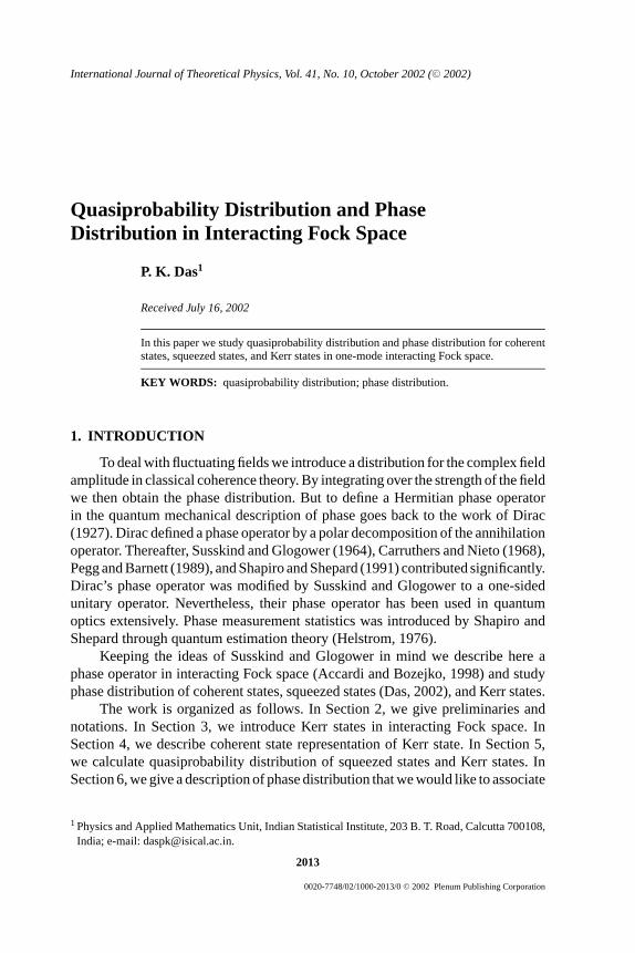
International Journal of Theoretical Physics, Vol. 41, No. 10, October 2002 ( C 2002) Quasiprobability Distribution and Phase Distribution in Interacting Fock Space P. K. Das 1 Received July 16, 2002 In this paper we study quasiprobability distribution and phase distribution for coherent states, squeezed states, and Kerr states in one-mode interacting Fock space. KEY WORDS: quasiprobability distribution; phase distribution. 1. INTRODUCTION To deal with fluctuating fields we introduce a distribution for the complex field amplitude in classical coherence theory. By integrating over the strength of the field we then obtain the phase distribution. But to define a Hermitian phase operator in the quantum mechanical description of phase goes back to the work of Dirac (1927). Dirac defined a phase operator by a polar decomposition of the annihilation operator. Thereafter, Susskind and Glogower (1964), Carruthers and Nieto (1968), Pegg and Barnett (1989), and Shapiro and Shepard (1991) contributed significantly. Dirac’s phase operator was modified by Susskind and Glogower to a one-sided unitary operator. Nevertheless, their phase operator has been used in quantum optics extensively. Phase measurement statistics was introduced by Shapiro and Shepard through quantum estimation theory (Helstrom, 1976). Keeping the ideas of Susskind and Glogower in mind we describe here a phase operator in interacting Fock space (Accardi and Bozejko, 1998) and study phase distribution of coherent states, squeezed states (Das, 2002), and Kerr states. The work is organized as follows. In Section 2, we give preliminaries and notations. In Section 3, we introduce Kerr states in interacting Fock space. In Section 4, we describe coherent state representation of Kerr state. In Section 5, we calculate quasiprobability distribution of squeezed states and Kerr states. In Section 6, we give a description of phase distribution that we would like to associate 1 Physics and Applied Mathematics Unit, Indian Statistical Institute, 203 B. T. Road, Calcutta 700108, India; e-mail: [email protected]. 2013 0020-7748/02/1000-2013/0 C 2002 Plenum Publishing Corporation
Transcript of Quasiprobability Distribution and Phase Distribution in Interacting Fock Space
P1: IBB
International Journal of Theoretical Physics [ijtp] pp647-ijtp-453633 November 6, 2002 20:24 Style file version May 30th, 2002
International Journal of Theoretical Physics, Vol. 41, No. 10, October 2002 (C© 2002)
Quasiprobability Distribution and PhaseDistribution in Interacting Fock Space
P. K. Das1
Received July 16, 2002
In this paper we study quasiprobability distribution and phase distribution for coherentstates, squeezed states, and Kerr states in one-mode interacting Fock space.
KEY WORDS: quasiprobability distribution; phase distribution.
1. INTRODUCTION
To deal with fluctuating fields we introduce a distribution for the complex fieldamplitude in classical coherence theory. By integrating over the strength of the fieldwe then obtain the phase distribution. But to define a Hermitian phase operatorin the quantum mechanical description of phase goes back to the work of Dirac(1927). Dirac defined a phase operator by a polar decomposition of the annihilationoperator. Thereafter, Susskind and Glogower (1964), Carruthers and Nieto (1968),Pegg and Barnett (1989), and Shapiro and Shepard (1991) contributed significantly.Dirac’s phase operator was modified by Susskind and Glogower to a one-sidedunitary operator. Nevertheless, their phase operator has been used in quantumoptics extensively. Phase measurement statistics was introduced by Shapiro andShepard through quantum estimation theory (Helstrom, 1976).
Keeping the ideas of Susskind and Glogower in mind we describe here aphase operator in interacting Fock space (Accardi and Bozejko, 1998) and studyphase distribution of coherent states, squeezed states (Das, 2002), and Kerr states.
The work is organized as follows. In Section 2, we give preliminaries andnotations. In Section 3, we introduce Kerr states in interacting Fock space. InSection 4, we describe coherent state representation of Kerr state. In Section 5,we calculate quasiprobability distribution of squeezed states and Kerr states. InSection 6, we give a description of phase distribution that we would like to associate
1 Physics and Applied Mathematics Unit, Indian Statistical Institute, 203 B. T. Road, Calcutta 700108,India; e-mail: [email protected].
2013
0020-7748/02/1000-2013/0C© 2002 Plenum Publishing Corporation

P1: IBB
International Journal of Theoretical Physics [ijtp] pp647-ijtp-453633 November 6, 2002 20:24 Style file version May 30th, 2002
2014 Das
to a given density operator. In Section 7, we give a few illustrative examples. Infact, we describe how the phase distribution will look like when we take coherentstates, squeezed states, and Kerr states in interacting Fock space. And finally inSection 8 we give a conclusion.
2. PRELIMINARIES AND NOTATIONS
As a vector space one-mode interacting Fock space0(C) is defined by
0(C) =∞⊕
n=0
C|n〉 (1)
whereC|n〉 is called then-particle subspace. The differentn-particle subspacesare orthogonal, that is, the sum in (1) is orthogonal. The norm of the vector|n〉 isgiven by
〈n | n〉 = λn (2)
where{λn}〉0. The norm introduced in (2) makes0(C) a Hilbert space.An arbitrary vectorf in 0(C) is given by
f ≡ c0|0〉 + c1|1〉 + c2|2〉 + · · · + cn|n〉 + . . . (3)
with ‖ f ‖ = (∑∞
n=0 |cn|2λn)1/2〈∞.We now consider the following actions on0(C):
a+|n〉 = |n+ 1〉
a|n+ 1〉 = λn+1
λn|n〉 (4)
a+ is called thecreation operatorand its adjointa is called theannihilationoperator. To define the annihilation operator we have taken the convention0/0= 0.
We observe that
〈n | n〉 = 〈a+(n− 1), n〉 = 〈(n− 1), an〉 = λn
λn−1〈n− 1, n− 1〉 = · · · (5)
and
‖|n〉‖2 = λn
λn−1.λn−1
λn−2· · · λ1
λ0= λn
λ0(6)
By (2) we observe from (6) thatλ0 = 1.The commutation relation takes the form
[a, a+] = λN+1
λN− λN
λN−1(7)
whereN is the number operator defined byN|n〉 = n|n〉.

P1: IBB
International Journal of Theoretical Physics [ijtp] pp647-ijtp-453633 November 6, 2002 20:24 Style file version May 30th, 2002
Quasiprobability Distribution and Phase Distribution in Interacting Fock Space 2015
3. GENERATION OF KERR STATE
The Kerr vectors in0(C) are defined by
φK (α) = ei2γa+a(a+a−1) fα (8)
where fα ∈ 0(C) is a coherent vector given by (6),γ is a constant, anda+a isdefined by
a+a|n〉 = λn
λn−1|n〉
Now,
φKα = e
i2γa+a(a+a−1) fα
= ei2γa+a(a+a−1)ψ(|α|2)−1/2
∞∑n=0
αn
λn|n〉
= ψ(|α|2)−1/2∞∑
n=0
αn
λne
i2γ
λnλn−1
( λnλn−1−1)|n〉
=∞∑
n=0
[ψ(|α|2)−1/2α
n
λne
i2γ
λnλn−1
( λnλn−1−1)]|n〉 =
∞∑n=0
qn|n〉 (9)
where
qn = ψ(|α|2)−1/2αn
λne
i2γ
λnλn−1
( λnλn−1−1) (10)
The photon number distribution
Pn =∣∣⟨n | φK
α
⟩∣∣2 = |qnλn|2
for the Kerr state is identical to that of the coherent state because the probabilityamplitudeqn andrn differ only by a phase factor.
4. COHERENT STATE REPRESENTATION
To obtain the coherent state representation of Kerr state8Kα we try to calculate
the matrix element (fα′ ,8Kα ), which contains all important information about the
state8Kα .
The matrix element is obtained by the following method. We utilize the com-pleteness relation of coherent state in0(C)
I =∫α∈C
dµ(α)| fα〉〈 fα|

P1: IBB
International Journal of Theoretical Physics [ijtp] pp647-ijtp-453633 November 6, 2002 20:24 Style file version May 30th, 2002
2016 Das
where
dµ(α) = ψ(|α|2)σ (|α|2)r dr dθ (11)
with α = r ei θ andσ (x) is some weight function.Now,
( fα′ , φKα ) = ( fα′ , U fα)
=∫α1∈C
dµ(α1) ( fα′ , U | fα1〉〈 fα1| fα)
=∫α1∈C
dµ(α1) ( fα1, fα) ( fα′ , U fα1) (12)
whereU ≡ ei2γa+a(a+a−1).
Now,
( fα1, fα) = ψ(|α|2)−1/2ψ(|α|2)−1/2∞∑
n=0
(α1)n(α)n
λn(13)
and
( fα′ , U fα1) = ψ(|α′|2)−1/2ψ(|α1|2)−1/2∞∑
n=0
(α′)n(α1)n
λne
i2γ
λnλn−1
( λnλn−1−1) (14)
Hence we have
( fα1, fα) ( fα′ , U fα1) = ψ(|α1|2)−1ψ(|α|2)−1/2ψ(|α′|2)−1/2
×∞∑
m,n=0
(α1)n(α)n
λn.(α′)m(α1)m
λme
i2γ
λmλm−1
( λmλm−1−1) (15)
Thus,(fα′ , φ
Kα
) = ∫α1∈C
dµ(α1) ( fα1, fα) ( fα′ , U fα1)
=∞∑
m=0,n=0
ψ(|α1|2)−1ψ(|α|2)−1/2ψ(|α′|2)−1/2(α′ )m(α)n
λmλn ei2γ
λmλm−1
( λmλm−1−1)
×∫α1∈C
dµ(α1)(α1)n(α1)m
=∞∑
n=0
ψ(|α|2)−1/2ψ(|α′|2)−1/2(α′ )n(α)n
λn ei2γ
λnλn−1
( λnλn−1−1) (16)
where we have utilized the fact∫∞
0 dxσ (x)xn = λnπ
(Das, 2002).

P1: IBB
International Journal of Theoretical Physics [ijtp] pp647-ijtp-453633 November 6, 2002 20:24 Style file version May 30th, 2002
Quasiprobability Distribution and Phase Distribution in Interacting Fock Space 2017
5. QUASIPROBABILITY DISTRIBUTION
Thequasiprobability distribution, known as theQ function, is the diagonalmatrix elements of the density operator in a pure coherent state
Q(α) = (α|ρ|α)
π(17)
We now calculate the quasiprobability distribution for the following states:
5.1. Squeezed States
For the squeezed statesf (Das, 2002),
f =[ ∞∑
n=0
|α|2n (λ1λ3λ5 · · · λ2n−1)2
(λ2λ4λ6 · · · λ2n−1)2λ2n
]−1/2 ∞∑n=0
αnλ1λ3λ5 · · · λ2n−1
λ2λ4λ6 · · · λ2n|2n〉 (18)
we take the density operator to be
ρ = | f 〉〈 f |, α = |α|ei θ0 (19)
and calculate the quasiprobability distributionQ(α′) as
Q(α′) = 1
π( f ′α, ρ f ′α)
= 1
π( fα′ , | f 〉〈 f | fα′ )
= 1
π|( fα′ , f )|2
= 1
π
∣∣∣∣ ∞∑n=0
α′2nαn λ1λ3λ5 · · · λ2n−1
λ2λ4λ6 · · · λ2n−2λ2nψ(|α′|2)−1/2
×[ ∞∑
n=0
|α|2n (λ1λ3λ5 · · · λ2n−1)2
(λ2λ4λ6 · · · λ2n−1)2λ2n
]−1/2 ∣∣∣∣∣2
(20)
5.2. Kerr States
For the Kerr statesφKα (9),
8Kα =
∞∑n=0
qn|n〉 (21)
where
qn = ψ(|α|2)−1/2αn
λne
i2γ
λnλn−1
( λnλn−1−1) (22)
P1: IBB
International Journal of Theoretical Physics [ijtp] pp647-ijtp-453633 November 6, 2002 20:24 Style file version May 30th, 2002
2018 Das
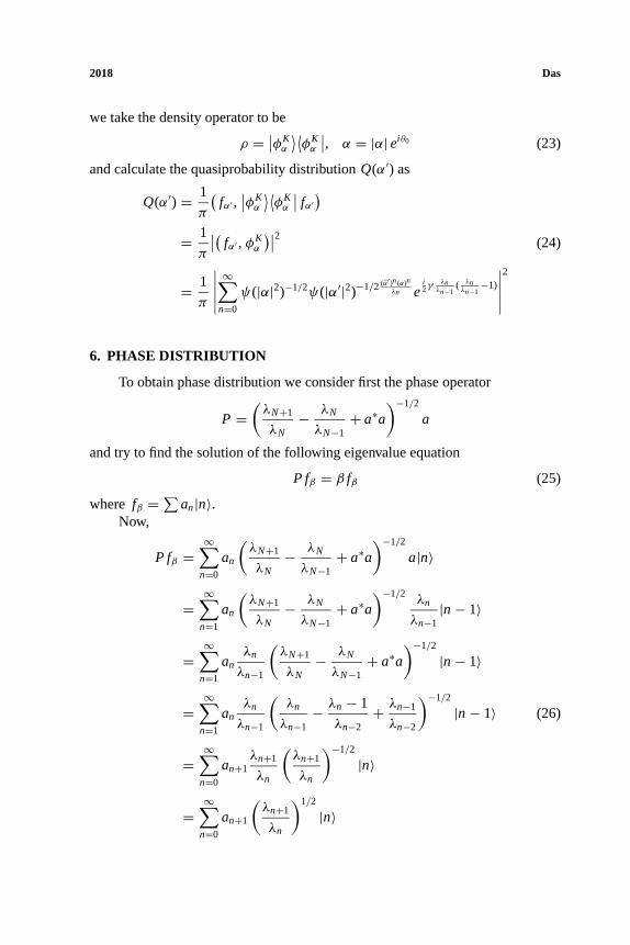
we take the density operator to be
ρ = ∣∣φKα
⟩ ⟨φKα
∣∣, α = |α| ei θ0 (23)
and calculate the quasiprobability distributionQ(α′) as
Q(α′) = 1
π
(fα′ ,
∣∣φKα
⟩ ⟨φKα
∣∣ fα′)
= 1
π
∣∣( fα′ , φKα
)∣∣2 (24)
= 1
π
∣∣∣∣∣ ∞∑n=0
ψ(|α|2)−1/2ψ(|α′|2)−1/2(α′ )n(α)n
λn ei2γ
λnλn−1
( λnλn−1−1)
∣∣∣∣∣2
6. PHASE DISTRIBUTION
To obtain phase distribution we consider first the phase operator
P =(λN+1
λN− λN
λN−1+ a∗a
)−1/2
a
and try to find the solution of the following eigenvalue equation
P fβ = β fβ (25)
where fβ =∑
an|n〉.Now,
P fβ =∞∑
n=0
an
(λN+1
λN− λN
λN−1+ a∗a
)−1/2
a|n〉
=∞∑
n=1
an
(λN+1
λN− λN
λN−1+ a∗a
)−1/2λn
λn−1|n− 1〉
=∞∑
n=1
anλn
λn−1
(λN+1
λN− λN
λN−1+ a∗a
)−1/2
|n− 1〉
=∞∑
n=1
anλn
λn−1
(λn
λn−1− λn − 1
λn−2+ λn−1
λn−2
)−1/2
|n− 1〉 (26)
=∞∑
n=0
an+1λn+1
λn
(λn+1
λn
)−1/2
|n〉
=∞∑
n=0
an+1
(λn+1
λn
)1/2
|n〉
P1: IBB
International Journal of Theoretical Physics [ijtp] pp647-ijtp-453633 November 6, 2002 20:24 Style file version May 30th, 2002
Quasiprobability Distribution and Phase Distribution in Interacting Fock Space 2019
β fβ =∞∑
n=0
βan|n〉 (27)
From (25)–(27) we see thatan satisfies the following difference equation:
an+1
(λn+1
λn
)1/2
= βan
That is
an+1 = β(λn+1
λn
)−1/2
an
Hence,
a1 = β(λ1
λ0
)−1/2
a0
a2 = β(λ2
λ1
)−1/2
a1 = β2
(λ2
λ1
)−1/2(λ1
λ0
)−1/2
a0 = β2
(λ2
λ0
)−1/2
a0
a3 = β(λ3
λ2
)−1/2
a2 = β3
(λ3
λ2
)−1/2(λ2
λ0
)−1/2
a0 = β3
(λ3
λ0
)−1/2
a0
and so on.Thus,
an = βn
(λn
λ0
)−1/2
a0 = βn(λn)−1/2a0
Hence
fβ =∞∑
n=0
an|n〉 = a0
∞∑n=0
βn(λn)−1/2|n〉
We takea0 = 1 andβ = |β| ei θ .Then
fβ =∞∑
n=0
einθ (λn)−1/2|β|n|n〉
Henceforth, we shall denote this vector as
fθ =∞∑
n=0
einθ (λn)−1/2|β|n|n〉
where 0≤ θ ≤ 2π and call fθ a phase vector in0(C).

P1: IBB
International Journal of Theoretical Physics [ijtp] pp647-ijtp-453633 November 6, 2002 20:24 Style file version May 30th, 2002
2020 Das
Norm of the phase vector is given by
‖ fθ‖2 =∞∑
m,n=0
einθeimθ (λn)−1/2(λm)1/2|β|n+m〈n | m〉
=∞∑
n=0
1
λn|β|2nλn =
∞∑n=0
|β|2n〈∞
(if |β| < 1).The phase vectors are complete. We can show that
I = 1
2π
∫X
∫ 2π
odν(x, θ )| fθ 〉〈 fθ | (28)
where
dν(x, θ ) = dµ(x) dθ (29)
Here we consider the setX consisting of the pointsx = 0, 1, 2,. . . , andµ(x) isthe measure onX which equals
µn = 1
|β|2n
at the pointx = n andθ is the Lebesgue measure on the circle.Define the operator
| fθ 〉〈 fθ | : 0(C)→ 0(C) (30)
by
| fθ 〉〈 fθ | f = ( fθ , f ) fθ (31)
with f =∑∞n=0 an|n〉.Now,
( fθ , f ) =∞∑
n=0
e−inθ (λn)1/2|β|nan
and
( fθ , f ) =∞∑
m,n=0
ei (m−n)θ (λm)−1/2|β|m(λn)1/2|β|nan|m〉
Hence
1
2π
∫X
∫ 2π
0dν(x, θ )| fθ 〉〈 fθ | f =
∫X
dµ(x)∑m,n
(λm)−1/2|β|m(λn)1/2|β|nan|m〉
P1: IBB
International Journal of Theoretical Physics [ijtp] pp647-ijtp-453633 November 6, 2002 20:24 Style file version May 30th, 2002
Quasiprobability Distribution and Phase Distribution in Interacting Fock Space 2021
× 1
2π
∫ 2π
0ei (m−n)θdθ
=∫
Xdµ(x)
∞∑n=0
|β|2n|n〉
=∞∑
n=0
an|n〉|β|2n 1
|β|2n
=∞∑
n=0
an|n〉
= f (32)
We use the vectorsfθ to associate to a given density operatorρ, a phasedistribution as follows:
P(θ ) = 1
2π( fθ , ρ fθ )
= 1
2π
∞∑m,n=0
|β|m|β|nei (n−m)
( |m〉√λm
, ρ|n〉√λm
)(33)
The P(θ ) as defined in (33) is positive, owing to the positivity ofρ, and isnormalized ∫
X
∫ 2π
0P(θ ) dν(x, θ ) = 1 (34)
where
dν(x, θ ) = dµ(x) dθ (35)
for, ∫X
∫ 2π
0P(θ ) dν(x, θ ) =
∫X
dµ(x)∞∑
m,n=0
|β|m|β|n 1
2π
∫ 2π
0
× ei (n−m)dθ
( |m〉√λm
, ρ|n〉√λn
)
=∫
Xdµ(x)
∞∑n=0
|β|2n
( |n〉√λn
, ρ|n〉√λn
)
=∞∑
n=0
( |n〉√λn
, ρ|n〉√λn
)= 1 (36)
P1: IBB
International Journal of Theoretical Physics [ijtp] pp647-ijtp-453633 November 6, 2002 20:24 Style file version May 30th, 2002
2022 Das
Thephase distributionover the window 0≤ θ ≤ 2π for any vectorf is thendefined by
P(θ ) = 1
2π|( fθ , f )|2
7. EXAMPLES
We now consider some important states in the Hilbert space0(C) and computetheir corresponding phase distributions.
7.1. Coherent States
For the coherent statesfα (Das, 2002),
fα = ψ(|α|2)−1/2∞∑
n=0
αn
λn|n〉 (37)
we take the density operator to be
ρ = | fα〉〈 fα|, α = |α| ei θ0 (38)
and calculate the phase distributionP(θ ) as
P(θ ) = 1
2π( fθ , ρ fθ )
= 1
2π( fθ , | fα〉〈 fα| fθ )
= 1
2π|( fθ , fα)|2 (39)
= 1
2π
∣∣∣∣∣ ∞∑n=0
ein(θ0−θ )|β|n|α|n(λn)−1/2ψ(|α|2)−1/2
∣∣∣∣∣2
7.2. Squeezed States
For the squeezed statesf (Das, 2002),
f =[ ∞∑
n=0
|α|2n (λ1λ3λ5 · · · λ2n−1)2
(λ2λ4λ6 · · · λ2n−1)2λ2n
]−1/2 ∞∑n=0
αnλ1λ3λ5 · · · λ2n−1
λ2λ4λ6 · · · λ2n|2n〉 (40)
we take the density operator to be
ρ = | f 〉〈 f |, α = |α| ei θ0 (41)

P1: IBB
International Journal of Theoretical Physics [ijtp] pp647-ijtp-453633 November 6, 2002 20:24 Style file version May 30th, 2002
Quasiprobability Distribution and Phase Distribution in Interacting Fock Space 2023
and calculate the phase distributionP(θ ) as
P(θ ) = 1
2π( fθ , ρ fθ )
= 1
2π( fθ , | f 〉〈 f | fθ )
= 1
2π|( fθ , f )|2 (42)
= 1
2π
∣∣∣∣ ∞∑n=0
ein(θ0−2θ )|β|2n|α|n λ1λ3λ5 · · · λ2n−1
λ2λ4λ6 · · · λ2n−2√λ2n
ψ(|α|2)−1/2
×[ ∞∑
n=0
|α|2n (λ1λ3λ5 · · · λ2n−1)2
(λ2λ4λ6 · · · λ2n−1)2λ2n
]−1/2 ∣∣∣∣2
7.3. Kerr States
For the Kerr statesφKα (9),
φKα =
∞∑n=0
qn|n〉 (43)
where
qn = ψ(|α|2)−1/2αn
λne
i2γ
λnλn−1
( λnλn−1−1) (44)
we take the density operator to be
ρ = ∣∣φKα
⟩ ⟨φKα
∣∣, α = |α| ei θ0 (45)
and calculate the phase distributionP(θ ) as
P(θ ) = 1
2π( fθ , ρ fθ )
= 1
2π
(fθ , |φK
α 〉〈φKα | fθ
)= 1
2π
∣∣( fθ , φKα
)∣∣2 (46)
= 1
2π
∣∣∣∣ ∞∑n=0
ein(θ0−θ )|β|n|α|n(λn)−1/2ψ(|α|2)−1/2ei2γ
λnλn−1
( λnλn−1−1)∣∣∣∣2

P1: IBB
International Journal of Theoretical Physics [ijtp] pp647-ijtp-453633 November 6, 2002 20:24 Style file version May 30th, 2002
2024 Das
8. CONCLUSION
In conclusion, we have first introduced Kerr states in the interacting Fockspace and studied quasiprobability distribution of squeezed states and Kerr statesin the space and then studied phase distribution in the space by defining a phaseoperator analogous to that studied by Susskind and Glogower and calculated spe-cific phase distributions in the case of coherent states, squeezed states, and Kerrstates.
REFERENCES
Accardi, L. and Bozejko, M. (1998). Interacting Fock Space and Gaussianization of Probability Mea-sures.Infinite Dimensional Analysis, Quantum Probability and Related Topics1(4), 663–670.
Accardi, L. and Nhani, M. (2001). The interacting Fock space of Haldane’s exclusion statistics.PreprintNo. 1.
Agarwal, G. S., Chaturvedi, S., Tara, K., and Srinivasan, V. (1992). Classical phase changes in nonlinearprocesses and their quantum counterparts,Physical Review A45, 4904.
Carruthers, P. and Nieto, M. M. (1968). Phase and angle variables in quantum mechanics.Reviews ofModern Physics40, 411.
Dirac, P. A. M. (1927).Proceedings of the Royal Society of London, Series A: Mathematical andPhysical Sciences114, 243.
Das, P. K. (2002). Coherent states and squeezed states in interacting Fock space.International Journalof Theoretical Physics41(6) 1099.
Helstrom, C. W. (1976).Quantum Detection and Estimation Theory, Academic Press, New York.Pegg, D. T. and Barnett, S. M. (1989). Unitary phase operator in quantum mechanics.Europhysics
Letters6, 483.Susskind, L. and Glogower, J. (1964).Physics1, 49.Shapiro, J. H. and Shepard, S. R. (1991). Quantum phase measurement: A system-theory perspective.
Physics Review A43, 3795.