Quasi stage order conditions for SDIRK methods

Applied Numerical Mathematics 42 (2002) 61–75www.elsevier.com/locate/apnum

Quasi stage order conditions for SDIRK methods

Frank Camerona,∗, Mikko Palmrothb, Robert Pichéb

a Pori School of Technology and Economics, P.O. Box 300, 28101 Pori, Finlandb Tampere University of Technology, P.O. Box 692, 33101 Tampere, Finland

Abstract

The stage order condition is a simplifying assumption that reduces the number of order conditions to be fulfilledwhen designing a Runge–Kutta (RK) method. Because a DIRK (diagonally implicit RK) method cannot have stageorder greater than 1, we introduce quasi stage order conditions and derive some of their properties for DIRKs. Weuse these conditions to derive a low-order DIRK method with embedded error estimator. Numerical tests with stiffODEs and DAEs of index 1 and 2 indicate that the method is competitive with other RK methods for low accuracytolerances. 2001 IMACS. Published by Elsevier Science B.V. All rights reserved.

Keywords:Differential–algebraic systems; Runge–Kutta methods

1. Introduction

Of all the classes of implicit Runge–Kutta methods (IRKs), diagonally implicit RK methods (DIRKs)are arguably the easiest to implement. In the past however, when DIRKs have been compared with otherIRKs in tests on DAEs, they have performed poorly [9,13]. One obvious reason for this is that DIRKstested were not originally designed for DAEs. In particular, they were not designed to attain a certainorder for DAEs.

To attain a certain order RK methods must satisfy order conditions. The stage order property is usefulsince it reduces the number of distinct order conditions. Other classes of IRKs used for solving DAEsusually have some stage order property as an integral part of their design [1,2,8]. However, DIRKscan only have the lowest stage order possible. This makes solving the order conditions for DIRKs anunappealing task. To remedy this situation for DIRKs, we use the concept of quasi stage order.

The idea behind quasi stage order is not new. Although they did not give it a name, Cooper andSayfy [5] used it in developing DIRKs for ODEs. Verner [16] called it dominant stage order and used it

* Corresponding author.E-mail address:[email protected] (F. Cameron).

0168-9274/01/$ – see front matter 2001 IMACS. Published by Elsevier Science B.V. All rights reserved.PII: S0168-9274(01)00142-8

62 F. Cameron et al. / Applied Numerical Mathematics 42 (2002) 61–75

to develop high-order explicit Runge–Kutta methods for ODEs. Our contribution is to extend the idea foruse in developing DIRKs for DAEs.

The paper is organised as follows. In Section 2 we give background notation and basic results. Thequasi stage order concepts are defined in Section 3, and various results for DIRKs are given. A DIRK thatwas derived using quasi stage order is presented in Section 4, together with some numerical test results.

2. Notation

2.1. DAEs

We are mainly interested in finding the numerical solution of the implicit index 1 differential algebraicequation (DAE) initial value problem

F(y′, y

)= 0, y(t0) = y0, y′(t0) = y′0, (1)

wherey :R → RN andF :RN ×R

N → RN . Although this DAE is autonomous, the discussion and results

apply equally for non-autonomous DAEs. We assume thaty is sufficiently differentiable. Kværnø [9]gives conditions for DAE (1) to be of index 1. A special case of (1) is the quasi-linear DAE

B(y)y′ − f (y) = 0, (2)

whereB(y) is singular.We will also be interested in solving the index 2 DAE initial value problem

y′ = f (y, z), y(t0) = y0 ∈ Rn, (3a)

0= g(y), z(t0) = z0 ∈ Rm. (3b)

This DAE has been widely researched [1,6,8]. It is known that the same Runge–Kutta (RK) method orderconditions are valid for both (1) and for they component of (3) [6, p. 506]. Thus if we have a candidatemethod for solving (1), then we can use it for solving for they component of (3), assuming the methodsatisfies any other requirements arising from (3).

2.2. Runge–Kutta methods

This section contains some RK terminology. Hairer and Wanner [6] should be consulted for moredetails.

Thestage variablesYi, i = 1,2, . . . , s, and thestage derivativesY ′j , j = 1,2, . . . , s, of ans-stage RK

method are related by

Yi = yn + h

s∑j=1

aij Y′j , i = 1,2, . . . , s. (4)

In (4) h is thestepsize. When (4) is applied to (1) the equation for stagei is

F

(Y ′i , yn + h

s∑j=1

aijY′j

)= 0, i = 1, . . . , s. (5)

F. Cameron et al. / Applied Numerical Mathematics 42 (2002) 61–75 63

Once all the stage derivatives have been computed the state can be updated using

yn+1 = yn + h

s∑i=1

biY′i . (6)

The parameters of an RK method are the matrixA ∈ Rs×s of (4) and the vectorb ∈ R

s×1 of (6). A FIRK(fully implicit RK method) has an invertibleA. We will useW � A−1. A DIRK (diagonally implicit RKmethod) is a FIRK whoseA is lower triangular. AnSDIRK (singularly diagonally implicit RK method)is a DIRK whoseA has one reals-fold eigenvalue.

We let y(tn+1) represent the exact solution of (1) after one time step when starting from consistentinitial conditions{tn, yn, y′

n}. Thelocal truncation error(LTE) for the RK solution of (6) and (5) is

δyn+1 � yn+1 − y(tn+1). (7)

The local orderof the RK method isκL if

δyn+1 = O(hκL). (8)

The LTE can be expressed as

δyn+1 =∞∑

i=κL

hi

(χi∑j=1

TijDij

), (9)

where theDij are elementary differentials or sums and products of partial differentials ofF . Thetruncation error coefficients(TECs)Tij are functions ofA, b and c. For an RK method to have localorderκL we must haveTij = 0, ∀j , i = 1, . . . , κL − 1. Typically however, anorder conditionis presentedas some multiple of its corresponding TEC, e.g.,αTij = 0, whereα makes the order condition neater.

We define theabscissaec ∈ Rs×1 of an RK method byc � Aes , wherees is as-vector of ones. Anon-

confluentRK method is one with distinctci .In anembedded RK pairthere is a secondb ∈ R

s×1 vector. The local order associated with the(A, b)-RK method isκL. AssumingκL andκL are different, then we can estimate the LTE from

|εn+1| �∣∣∣∣∣h

s∑i=1

(bi − bi

)Y ′i

∣∣∣∣∣≈ |δyn+1|. (10)

We assume that the(A, b)-RK method is used for updating the state via (6). We refer to the(A, b) and(A, b)-RK methods as theupdatingand theauxiliary methods, respectively.

There is a one-to-one correspondence between order conditions and certain trees. Theorder of treet

is denotedρ(t). An RK method has local orderκL when all order conditions are satisfied for trees havingρ(t) � κL − 1. Table 1 contains the trees forρ(t) � 4. The notationt = [t1, . . . , tk, u1, . . . , u%]y meansthe tree obtained by connecting the roots oft1, . . . , tk, u1, . . . , u% to a new light vertex, which becomesthe root of treet . Analogously,u = [t1, . . . , tk]z indicates the tree obtained by connecting the roots oft1, . . . , tk to a new heavy vertex, which becomes the root of treeu. Further details on trees and theircorresponding order conditions can be found in Kværnø [9].


Table 1The order trees up toρ(t)= 4. The root vertex is labelled byξr


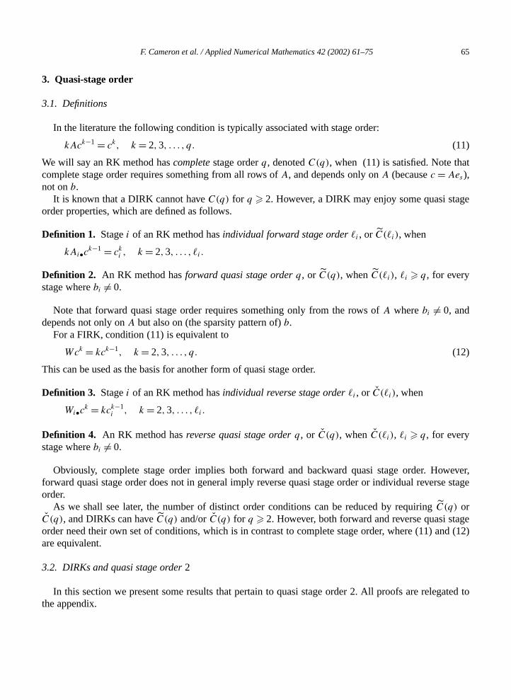
3. Quasi-stage order

3.1. Definitions

In the literature the following condition is typically associated with stage order:

kAck−1 = ck, k = 2,3, . . . , q. (11)

We will say an RK method hascompletestage orderq, denotedC(q), when (11) is satisfied. Note thatcomplete stage order requires something from all rows ofA, and depends only onA (becausec = Aes ),not onb.

It is known that a DIRK cannot haveC(q) for q � 2. However, a DIRK may enjoy some quasi stageorder properties, which are defined as follows.

Definition 1. Stagei of an RK method hasindividual forward stage order%i , or C(%i), when

kAi•ck−1 = cki , k = 2,3, . . . , %i.

Definition 2. An RK method hasforward quasi stage orderq, or C(q), whenC(%i), %i � q, for everystage wherebi �= 0.

Note that forward quasi stage order requires something only from the rows ofA wherebi �= 0, anddepends not only onA but also on (the sparsity pattern of)b.

For a FIRK, condition (11) is equivalent to

Wck = kck−1, k = 2,3, . . . , q. (12)

This can be used as the basis for another form of quasi stage order.

Definition 3. Stagei of an RK method hasindividual reverse stage order%i , or C(%i), when

Wi•ck = kck−1i , k = 2,3, . . . , %i.

Definition 4. An RK method hasreverse quasi stage orderq, or C(q), whenC(%i), %i � q, for everystage wherebi �= 0.

Obviously, complete stage order implies both forward and backward quasi stage order. However,forward quasi stage order does not in general imply reverse quasi stage order or individual reverse stageorder.

As we shall see later, the number of distinct order conditions can be reduced by requiringC(q) orC(q), and DIRKs can haveC(q) and/orC(q) for q � 2. However, both forward and reverse quasi stageorder need their own set of conditions, which is in contrast to complete stage order, where (11) and (12)are equivalent.

3.2. DIRKs and quasi stage order2

In this section we present some results that pertain to quasi stage order 2. All proofs are relegated tothe appendix.


We will use the following partition:

A =[A1 0A2 A3

], W =

[W1 0W2 W3

], b =

[0β2

], c =

[γ1

γ2

], (13)

whereA1 ∈ Rr×r , A3 ∈ R

(s−r)×(s−r), and the other matrices are appropriately dimensioned.Row 2 of a DIRK can have eitherC(2) or C(2), but not both. This restriction can be seen when we

parameterize the first 2 rows ofA andW as follows:[A1•A2•

]=[

a11 0 0 . . . 0c2 − a22 a22 0 . . . 0

],[

W1•W2•

]=[

1/a11 0 0 . . . 0(a22 − c2)/(a11a22) 1/a22 0 . . . 0

].

With this parameterization the conditions forC(2) andC(2) for row 2 are

c22/2= (c2 − a22)a11 + a22c2, (14)

2c2a11a22 = (a22 − c2)c21 + a11c

22. (15)

It can be shown that all solutions of (14), (15) imply a singularA and hence are not permissible.Another restriction is the following.

Lemma 5. If a DIRK is stiffly accurate, has forward quasi stage orderC(2) and has anA matrix whoselast row is

As• = [0 0 . . . 0 1− ass ass],then this DIRK cannot haveκL = 5, even for ODEs.

Both forward and reverse quasi stage order make redundant some of the order conditions correspond-ing to the trees of Table 1. If a DIRK hasC(2), then the redundant order conditions are those correspond-ing to trees having the formt = [t2, t (η)]y wheret2 is given in Table 1 andt (η) are all other branches inthe remainder of the tree. The order condition for this tree has the form

bT[Ac � η] = 1/λ(t)

From Definition 2 and (13) we can rewrite this order condition as[0 βT

2

]([A1γ1

γ 22 /2

]�[η1

η2

])= βT

2

[(γ 2

2 /2)� η2

]= 1

2bT(c2 � η

)= 1/λ(t).

This expression corresponds to the treet = [t1, t1, t (η)]y .The order conditions made redundant by reverse quasi stage order 2,C(2), are those whose tree has

the formt = [u1, t (η)]y , where

u1 =and t (η) are all other branches in the remainder of the tree. The order condition for such a tree has theform

bT[Wc2 � η

]= 1/λ(t).


Table 2The number of distinct order conditions given various properties

To attain local order Number distinct order conditions when RK method has properties

κL no stiff C(2) and C(2) and C(2), C(2)properties acc. stiff acc. stiff acc. and stiff acc.

4 9 6 4 3 2

5 30 20 16 11 9

From Definition 4 and (13) we can rewrite this order condition as[0 βT

2

]([W1γ21

2γ2

]�[η1

η2

])= βT

2

[(2γ2) � η2

]= 2bT(c � η) = 1/λ(t).

This expression corresponds to the treet = [t1, t (η)]y .If we combine forward or reverse quasi stage order with stiff accuracy, we can further reduce the

number of distinct order conditions. Stiff accuracy makes redundant all order conditions correspondingto trees of the form[[t1, . . . , tk]z]y . Table 2 gives the number of distinct order conditions for varioussituations. In particular, if a DIRK is required to have stiff accuracy,C(2), andC(2), then of the 30 treesof Table 1 all but the following 9 are redundant:t1, t4, t10, t12, t13, t14, t15, t19 andt20.

3.3. General results on quasi stage order

In this section we present some general results on quasi stage order.It follows directly from Definition 2 that if a DIRK is stiffly accurate and hasC(q), then it satisfies the

order conditions

bTck = 1/(k + 1), k = 1,2, . . . , q.

Similar order conditions arise from DAEs:

bTWck = 1.

However, any stiffly accurate FIRK will satisfy all order conditions of this latter form; we need notrequire reverse quasi stage orderC(q).

The next lemma shows that separate conditions forC(%) andC(%) are not needed for rows of A.

Lemma 6. If a DIRK is stiffly accurate, hasC(%) and the partition of(13) holds, then rows of the DIRKhasC(%).

The next two lemmas give sufficient conditions for SDIRKs to have individual forward and reversestage order.

Lemma 7. Let ai2, ai3, . . . , aiq be free parameters inAi• of a non-confluent SDIRK. By setting theseparameters rowi can haveC(q) for i > q.

Lemma 8. Assume that for alli, ci �= 0. Let wi2,wi3, . . . ,wiq be free parameters inWi• of a non-confluent SDIRK. By setting these parameters rowi can haveC(q) for i > q.


In the proof of Lemma 7 there were no restrictions on the elements ofAi•. However, in a stiffly accurateSDIRKAs• is constrained by partition (13), i.e., the firstr elements ofAs• are zero. The following lemmashows what is attainable for rows in this situation.

Lemma 9. Letas,r+2, as,r+3, . . . , ass be free parameters inAs• of a non-confluent, stiffly accurate SDIRK.By setting these parameters rows can haveC(q) for s − r � q.

Lemma 10. Assume that for alli, ci �= 0. Let ws,r+2,ws,r+3, . . . ,wss be free parameters inWs• of anon-confluent stiffly accurate SDIRK. By setting these parameters rows can haveC(q) for s − r � q.

Combining Lemmas 7 and 9 we get:

Theorem 11. An s-stage stiffly accurate SDIRK can haveC(q) for s = 2q.

Similarly, we can combine Lemmas 8 and 10 to get

Theorem 12. An s-stage stiffly accurate SDIRK can haveC(q) for s = 2q.

We expect that in practice individual stage orders for SDIRKs will never need to exceed 3. We havefound it possible to attain bothC(p) andC(q) for row i whenp + q − 1 � i, 1� p � 3 and 1� q � 3.Forp + q − 1= i however, we must assume there is one free parameter from some rowj , j < i.

4. A new SDIRK embedded pair

We used quasi stage order in designing the new SDIRK pair, denoted SDIRK2, given by the followingButcher table:

1/4 1/4 0 0 011/28 1/7 1/4 0 01/3 61/144 −49/144 1/4 01 0 0 3/4 1/4

bT 0 0 3/4 1/4bT −61/600 49/600 79/100 23/100

(16)

We required the updating SDIRK(A, b) to be stiffly accurate, which impliesg(yn) = 0 for (3), thatis, the algebraic constraints are satisfied at the end of each RK step. We also required bothC(2)and C(2). After satisfying the two distinct order conditions remaining (see Table 2), we obtained anupdating SDIRK withκL = 4. The auxiliary (A, b) SDIRK has κL = 3, so the local error can beestimated from (10). The updating(A, b) SDIRK is L-stable; this removes one source in the errorpropagation of FIRKs [7, Theorem 4.4] and in addition impliesA-stability. The auxiliary(A, b) SDIRKis A-stable.


Table 3Performance measures for the SDIRK pairs

Pair χ(−∞) γ (−∞) υ1 υ2 ‖4dT‖2

SDIRK1 0 0.12 1.0 1.5 1.4

SDIRK2 0.39 0 1.7 1.8 1.9

We also considered the following quality measures for RK methods.

• Cameron [3] suggests that to obtain a good local error estimate for stiff problems,χ(−∞) should besmall andγ (−∞) should be in the range(0.1,1), where

γ (z)�∣∣exp(z)− R(z)

∣∣/∣∣R(z)− R(z)∣∣, (17a)

χ(z) �∣∣R(z)−R(z)

∣∣ (17b)

andR(z) � 1+ zbT(I − zA)−1es is the standard stability function.• Shampine [15, pp. 374–375] suggests that to obtain a good local error estimate for stiff problems, the

measures

υ1 � ‖TκL+1,•‖/‖TκL,•‖, (18)

υ2 �∥∥TκL+1,• − TκL+1,•

∥∥/‖TκL,•‖ (19)

should be small. We choose to use the∞-norm.• Nørsett and Thomsen [11] suggest that if∥∥4dT

∥∥�∥∥(bT − bT

)A−1

∥∥ (20)

is small, then a more lax stopping criterion may be used with the iterative (e.g., Newton) solver, sothat less work is needed in this part of the method.

Table 3 contains the values of these performance measures for SDIRK2. For comparison, we show theperformance measures for the four stage method 2b from [4], here denoted SDIRK1. These measures allfavour SDIRK1. However, numerical test results presented later tend to favour SDIRK2.

However, for solving the index 2 DAE (3), SDIRK2 is preferable, because it can at least attain localorder κL = 2 for z, whereas SDIRK1 cannot. There is one order condition needed to obtainκL = 2for z:

bTW 2c2 = 2.

The(A, b) SDIRK in SDIRK2 satisfies this; neither SDIRK in SDIRK1 does.

5. Tests

Numerical tests on six small ODE and DAE problems (Table 4) were performed using Olsson’s C++solver package Godess [12] running under Windows NT on an Intel PIII CPU. Most of the examples arestiff ODE or DAE benchmark problems from the literature [6,10]. The hydraulics examples are small


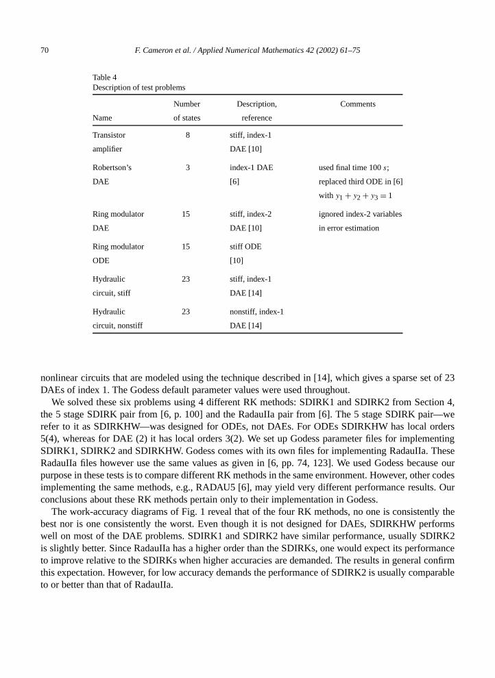
Table 4Description of test problems

Number Description, Comments

Name of states reference

Transistor 8 stiff, index-1

amplifier DAE [10]

Robertson’s 3 index-1 DAE used final time 100s;

DAE [6] replaced third ODE in [6]

with y1 + y2 + y3 = 1

Ring modulator 15 stiff, index-2 ignored index-2 variables

DAE DAE [10] in error estimation

Ring modulator 15 stiff ODE

ODE [10]

Hydraulic 23 stiff, index-1

circuit, stiff DAE [14]

Hydraulic 23 nonstiff, index-1

circuit, nonstiff DAE [14]

nonlinear circuits that are modeled using the technique described in [14], which gives a sparse set of 23DAEs of index 1. The Godess default parameter values were used throughout.

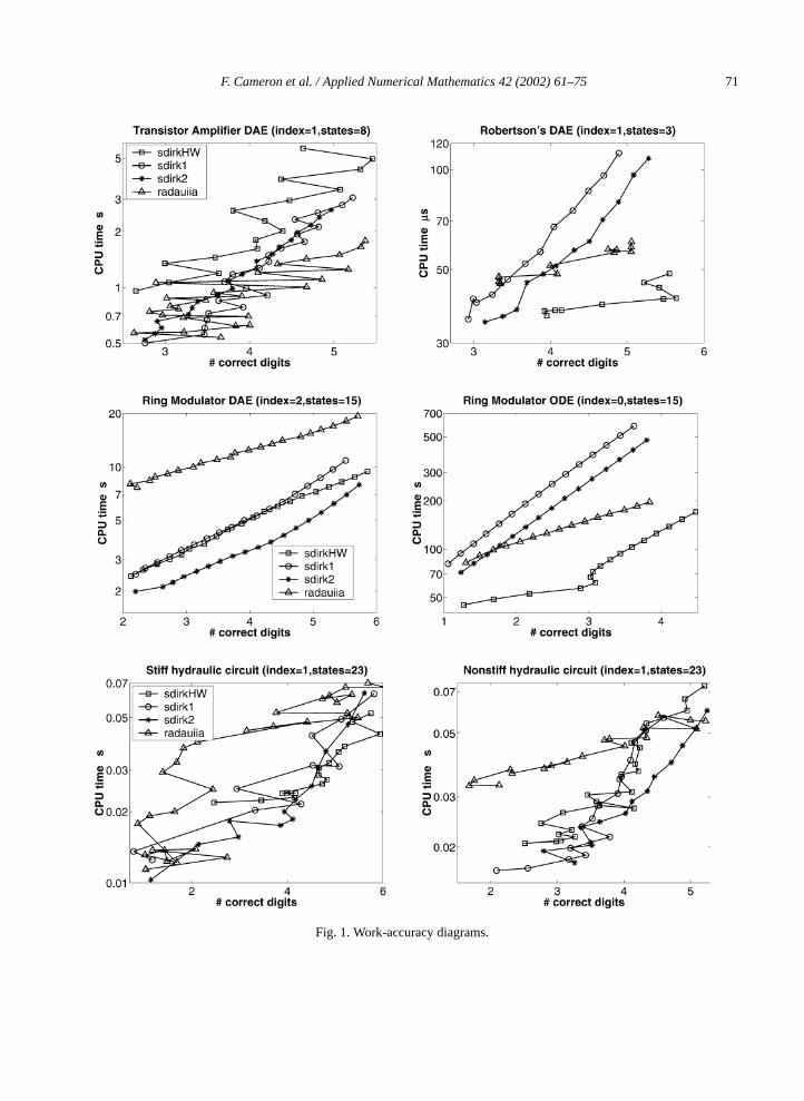
We solved these six problems using 4 different RK methods: SDIRK1 and SDIRK2 from Section 4,the 5 stage SDIRK pair from [6, p. 100] and the RadauIIa pair from [6]. The 5 stage SDIRK pair—werefer to it as SDIRKHW—was designed for ODEs, not DAEs. For ODEs SDIRKHW has local orders5(4), whereas for DAE (2) it has local orders 3(2). We set up Godess parameter files for implementingSDIRK1, SDIRK2 and SDIRKHW. Godess comes with its own files for implementing RadauIIa. TheseRadauIIa files however use the same values as given in [6, pp. 74, 123]. We used Godess because ourpurpose in these tests is to compare different RK methods in the same environment. However, other codesimplementing the same methods, e.g., RADAU5 [6], may yield very different performance results. Ourconclusions about these RK methods pertain only to their implementation in Godess.

The work-accuracy diagrams of Fig. 1 reveal that of the four RK methods, no one is consistently thebest nor is one consistently the worst. Even though it is not designed for DAEs, SDIRKHW performswell on most of the DAE problems. SDIRK1 and SDIRK2 have similar performance, usually SDIRK2is slightly better. Since RadauIIa has a higher order than the SDIRKs, one would expect its performanceto improve relative to the SDIRKs when higher accuracies are demanded. The results in general confirmthis expectation. However, for low accuracy demands the performance of SDIRK2 is usually comparableto or better than that of RadauIIa.


Fig. 1. Work-accuracy diagrams.


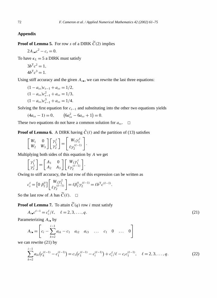
Appendix

Proof of Lemma 5. For rows of a DIRK C(2) implies

2As•c2 − cs = 0.

To haveκL = 5 a DIRK must satisfy

3bTc2 = 1,

4bTc3 = 1.

Using stiff accuracy and the givenAs•, we can rewrite the last three equations:

(1− ass)cs−1 + ass = 1/2,

(1− ass)c2s−1 + ass = 1/3,

(1− ass)c3s−1 + ass = 1/4.

Solving the first equation forcs−1 and substituting into the other two equations yields

(4ass − 1) = 0,(6a2

ss − 6ass + 1)= 0.

These two equations do not have a common solution forass . ✷Proof of Lemma 6. A DIRK having C(%) and the partition of (13) satisfies[

W1 0W2 W3

][γ %

1γ %

2

]=[

W1γ%1

%γ(%−1)2

].

Multiplying both sides of this equation byA we get[γ %

1γ %

2

]=[A1 0A2 A3

][W1γ

%1

%γ(%−1)2

].

Owing to stiff accuracy, the last row of this expression can be written as

c%s = [0 βT

2

][ W1γ21

%γ(%−1)2

]= %βT

2 γ(%−1)2 = %bTc(%−1).

So the last row ofA hasC(%). ✷Proof of Lemma 7. To attainC(q) row i must satisfy

Ai•c%−1 = c%i /%, % = 2,3, . . . , q. (21)

ParameterizingAi• by

Ai• =[ci −

i−1∑k=2

aik − c1 ai2 ai3 . . . c1 0 . . . 0

]we can rewrite (21) by

i−1∑k=2

aik(c(%−1)k − c

(%−1)1

)= c1(c(%−1)1 − c

(%−1)i

)+ c%i /%− cic(%−1)1 , % = 2,3, . . . , q. (22)


Assumingq < i, then from (22) we can set up a linear equation set to solve for[ai2 ai3 . . . aiq ]. The(q − 1) × (q − 1) coefficient matrix for this linear equation set is

c2 − c1 c3 − c1 . . . cq − c1

c22 − c2

1 c23 − c2

1 . . . c2q − c2

1...

...

c(q−1)2 − c

(q−1)1 c

(q−1)3 − c

(q−1)1 . . . c

(q−1)q − c

(q−1)1

= V22 − V21V12 (23)

where[

1 V12V21 V22

]is the transpose of the Vandermonde matrix for[c1, . . . , cq]. The Vandermonde matrix

(and hence the coefficient matrix (23)) is invertible iff the abscissaec1, c2, c3, . . . , cq are distinct. ✷Proof of Lemma 8. The parameterization ofWi• we will use is

Wi• =[c−2

1

(c1 − c1

i−1∑k=2

wikck − ci

)wi2 wi3 . . . c−1

1 0 . . . 0

]. (24)

Row i hasC(q) when the following are satisfied:

Wi•c% = %c%−1i , % = 2,3, . . . , q. (25)

Using (24) we can rewrite (25) as

i−1∑k=2

wikck(c(%−1)k−1 − c

(%−1)1

)= c(%−2)i − c

(%−1)1 + %c

(%−1)i − c%i /c1, % = 2,3, . . . , q. (26)

Assumingq < i, then from (22) we can set up a linear equation set to solve for[wi2 wi3 . . . wiq]. The(q − 1) × (q − 1) matrix for this linear equation set can be written as

c2 − c1 c3 − c1 . . . cq − c1

c22 − c2

1 c23 − c2

1 . . . c2q − c2

1...

...

c(q−1)2 − c

(q−1)1 c

(q−1)3 − c

(q−1)1 . . . c

(q−1)q − c

(q−1)1

c2 0 . . . 00 c3 . . . 0...

. . ....

0 0 . . . cq

. (27)

We can use the same reasoning as in the proof of Lemma 7 to argue that non-confluency andci �= 0 aresufficient for this matrix to be invertible. ✷Proof of Lemma 9. We will only consider the case ofq = s − r .

Let As• be given by

As• =[

0 0 . . . 0 1−s−1∑

k=r+2

ask − ass as,r+2 as,r+3 . . . ass

].

The conditions we need to satisfy are given by (21) withi = s andci = 1. We can write these conditionsas

ass(1− c

(%−1)r+1

)+s−1∑

k=r+2

ask(c(%−1)k − c

(%−1)r+1

)= 1/% − c(%−1)r+1 , % = 2,3, . . . , q. (28)


If we set up the linear equation set to solve for[as,r+2 as,r+3 . . . ass], then the corresponding(s − r − 1) × (s − r − 1) matrix is

cr+2 − cr+1 cr+3 − cr+1 . . . 1− cr+1

c2r+2 − c2

r+1 c2r+3 − c2

r+1 . . . 1− c2r+1

......

c(q−1)r+2 − c

(q−1)r+1 c

(q−1)r+3 − c

(q−1)r+1 . . . 1− c

(q−1)r+1

.

We can use the same reasoning as in the proof of Lemma 7 to argue that non-confluency is sufficient forthis matrix to be invertible. ✷Proof of Lemma 10. The proof of Lemma 9 uses the framework of the proof of Lemma 7 with thefollowing condition: we may solve only for the lasts−r−1 elements ofAs•, which includes the diagonalelement. In the same sense we can prove Lemma 10 using the framework of the proof of Lemma 8.✷Proof of Theorem 11. Consider a stiffly accurate SDIRK designed with the following properties:(i) rows q + 1, q + 2, . . . , s − 1 haveC(q), (ii) row s hasC(q), and (iii) the firstq elements ofAs•are zero. Property (i) is possible from Lemma 7. Property (iii) and the partition of (13) impliesr = q.Fromr = q and Lemma 9, property (ii) is possible whens � q + r = 2q. From Definition 2 this SDIRKhasC(q). ✷Proof of Theorem 12. Analogous to the proof of Theorem 11.✷

References

[1] A. Aubry, P. Chartier, On improving the convergence of Radau IIA methods applied to index 2 DAEs, SIAM J. Numer.Anal. 35 (1998) 1347–1367.

[2] J.C. Butcher, R.P.K. Chan, Efficient Runge–Kutta integrators for index 2 differential algebraic equations, Math. Comp. 67(1998) 1001–1021.

[3] F. Cameron, A class of low order DIRK methods for a class of DAEs, Appl. Numer. Math. 31 (1999) 1–16.[4] F. Cameron, Low-order Runge–Kutta methods for differential-algebraic equations, Ph.D. Thesis, Tampere University of

Technology, Tampere, Finland, 1999.[5] G.J. Cooper, A. Sayfy, Semi-explicit A-stable Runge–Kutta methods, Math. Comp. 33 (1979) 541–556.[6] E. Hairer, G. Wanner, Solving Ordinary Differential Equations II, Stiff and Differential–Algebraic Problems, Springer Ser.

Comput. Math., Vol. 14, Springer, Berlin, 1996.[7] E. Hairer, C. Lubich, M. Roche, The Numerical Solution of Differential–Algebraic Systems by Runge–Kutta Methods,

Lecture Notes in Math., Vol. 1409, Springer, Berlin, 1989.[8] L. Jay, Convergence of a class of Runge–Kutta methods for differential algebraic systems of index 2, BIT 33 (1993)

137–150.[9] A. Kværnø, Runge–Kutta methods applied to fully implicit differential–algebraic equations of index 1, Math. Comput. 54

(1990) 583–625.[10] W.M. Lioen, J.J.B. de Swart, Test set for initial value problem solvers, CWI Report MAS-R9832, Amsterdam, The

Netherlands, 1998; http://www.cwi.nl/cwi/projects/IVPtestset/.[11] S.P. Nørsett, P.G. Thomsen, Local error control in SDIRK-methods, BIT 26 (1986) 100–113.[12] H. Olsson, Runge–Kutta solution of initial value problems, methods, algorithms and implementation, Ph.D. Thesis, Lund

University, Lund, Sweden, 1998.[13] L.R. Petzold, Order results for implicit Runge–Kutta methods applied to differential/algebraic systems, SIAM J. Numer.

Anal. 23 (1986) 837–852.


[14] R. Piché, M. Palmroth, Modular modelling using Lagrangian DAEs, in: S.S. Nair (Ed.), Proceedings of the ASMEInternational Mechanical Engineering Congress and Exposition, Orlando, Florida, Volume 69-2, 2000, pp. 755–761.

[15] L.F. Shampine, Numerical Solution of Ordinary Differential Equations, Chapman & Hall, New York, 1994.[16] J.H. Verner, High-order explicit Runge–Kutta pairs with low stage order, Appl. Numer. Math. 22 (1996) 345–357.

Quasi stage order conditions for SDIRK methods

Documents

Transcript of Quasi stage order conditions for SDIRK methods