QuantumComputing,Quantum GamesandGeometricAlgebra · QuantumComputing,Quantum...
138
Quantum Computing, Quantum Games and Geometric Algebra James M. Chappell The School of Chemistry and Physics, University of Adelaide, Australia October 29, 2011
Transcript of QuantumComputing,Quantum GamesandGeometricAlgebra · QuantumComputing,Quantum...

Quantum Computing, Quantum
Games and Geometric Algebra
James M. Chappell
The School of Chemistry and Physics,
University of Adelaide,
Australia
October 29, 2011

Contents
1 Introduction 1
1.1 Overview of thesis . . . . . . . . . . . . . . . . . . . . . . . . . . . . . . . . . . 21.2 Basic principles of quantum computers . . . . . . . . . . . . . . . . . . . . . . . 3
1.2.1 Tensor product notation . . . . . . . . . . . . . . . . . . . . . . . . . . . 41.3 Geometric algebra (GA) . . . . . . . . . . . . . . . . . . . . . . . . . . . . . . . 4
1.3.1 The vector cross product and quaternions . . . . . . . . . . . . . . . . . 51.3.2 Generalizations beyond quaternions . . . . . . . . . . . . . . . . . . . . 51.3.3 Clifford’s geometric algebra . . . . . . . . . . . . . . . . . . . . . . . . . 51.3.4 Geometric algebra (GA) in 3 dimensions . . . . . . . . . . . . . . . . . . 61.3.5 Rotations in 3-space with GA . . . . . . . . . . . . . . . . . . . . . . . . 71.3.6 Representing quantum states in GA . . . . . . . . . . . . . . . . . . . . 71.3.7 Measurement probabilities in GA . . . . . . . . . . . . . . . . . . . . . . 8
1.4 Java software development . . . . . . . . . . . . . . . . . . . . . . . . . . . . . . 81.5 Quantum Gates . . . . . . . . . . . . . . . . . . . . . . . . . . . . . . . . . . . . 11
1.5.1 Single qubit gates . . . . . . . . . . . . . . . . . . . . . . . . . . . . . . 111.5.2 Single qubit gates in geometric algebra . . . . . . . . . . . . . . . . . . . 121.5.3 Two qubit gates . . . . . . . . . . . . . . . . . . . . . . . . . . . . . . . 141.5.4 Three qubit gates . . . . . . . . . . . . . . . . . . . . . . . . . . . . . . . 151.5.5 Measurements . . . . . . . . . . . . . . . . . . . . . . . . . . . . . . . . 15
1.6 General quantum circuits . . . . . . . . . . . . . . . . . . . . . . . . . . . . . . 161.6.1 Copying circuit . . . . . . . . . . . . . . . . . . . . . . . . . . . . . . . . 161.6.2 Creating a Bell state or an EPR pair . . . . . . . . . . . . . . . . . . . . 171.6.3 Quantum parallelism . . . . . . . . . . . . . . . . . . . . . . . . . . . . . 18
1.7 Summary of quantum algorithms . . . . . . . . . . . . . . . . . . . . . . . . . . 19
2 The Fourier Transform and the Phase Estimation Algorithm 21
2.1 Quantum Fourier transform (QFT) . . . . . . . . . . . . . . . . . . . . . . . . . 212.1.1 Definition of the Fourier transform . . . . . . . . . . . . . . . . . . . . . 212.1.2 Definition of binary expansion . . . . . . . . . . . . . . . . . . . . . . . 212.1.3 Rearranging the Fourier transform formula . . . . . . . . . . . . . . . . 22
2.2 Phase estimation . . . . . . . . . . . . . . . . . . . . . . . . . . . . . . . . . . . 232.3 Reliability of Estimate . . . . . . . . . . . . . . . . . . . . . . . . . . . . . . . . 24
2.3.1 Introduction . . . . . . . . . . . . . . . . . . . . . . . . . . . . . . . . . 242.3.2 Accuracy formula . . . . . . . . . . . . . . . . . . . . . . . . . . . . . . . 252.3.3 Special cases . . . . . . . . . . . . . . . . . . . . . . . . . . . . . . . . . 282.3.4 Summary . . . . . . . . . . . . . . . . . . . . . . . . . . . . . . . . . . . 29
3 Grover’s Algorithm 31
3.1 Grover’s search algorithm . . . . . . . . . . . . . . . . . . . . . . . . . . . . . . 313.1.1 Performance . . . . . . . . . . . . . . . . . . . . . . . . . . . . . . . . . 343.1.2 Quantum counting . . . . . . . . . . . . . . . . . . . . . . . . . . . . . . 353.1.3 Two-step starting probability distributions . . . . . . . . . . . . . . . . 363.1.4 A single pass search using phase estimation . . . . . . . . . . . . . . . . 38
3.2 Quantum search using a Hamiltonian . . . . . . . . . . . . . . . . . . . . . . . . 403.3 The Grover Search using SU(2) rotations . . . . . . . . . . . . . . . . . . . . . 42
3.3.1 The Grover search space . . . . . . . . . . . . . . . . . . . . . . . . . . . 433.3.2 SU(2) generators for the Grover search space . . . . . . . . . . . . . . . 44
i

3.3.3 Analogy to spin precession . . . . . . . . . . . . . . . . . . . . . . . . . 47
3.3.4 Exact search . . . . . . . . . . . . . . . . . . . . . . . . . . . . . . . . . 49
3.3.5 Application: developing a circuit . . . . . . . . . . . . . . . . . . . . . . 51
3.4 Summary . . . . . . . . . . . . . . . . . . . . . . . . . . . . . . . . . . . . . . . 53
4 The Grover Search using Geometric Algebra 55
4.1 The Grover search operator in GA . . . . . . . . . . . . . . . . . . . . . . . . . 56
4.1.1 Exact Grover search . . . . . . . . . . . . . . . . . . . . . . . . . . . . . 57
4.1.2 General exact Grover search . . . . . . . . . . . . . . . . . . . . . . . . . 61
4.2 Summary . . . . . . . . . . . . . . . . . . . . . . . . . . . . . . . . . . . . . . . 62
5 Quantum Game Theory 63
5.1 Constructing quantum games from symmetric non-factorisable joint probabilities 66
5.2 The penny flip quantum game and geometric algebra . . . . . . . . . . . . . . . 67
6 Two-player Quantum Games 69
6.1 Introduction . . . . . . . . . . . . . . . . . . . . . . . . . . . . . . . . . . . . . . 69
6.2 EPR setting for playing a quantum game . . . . . . . . . . . . . . . . . . . . . 70
6.3 Geometric algebra . . . . . . . . . . . . . . . . . . . . . . . . . . . . . . . . . . 71
6.3.1 Calculating observables . . . . . . . . . . . . . . . . . . . . . . . . . . . 72
6.3.2 Finding the payoff relations . . . . . . . . . . . . . . . . . . . . . . . . . 74
6.3.3 Solving the general two-player game . . . . . . . . . . . . . . . . . . . . 74
6.3.4 Embedding the classical game . . . . . . . . . . . . . . . . . . . . . . . . 75
6.4 Examples . . . . . . . . . . . . . . . . . . . . . . . . . . . . . . . . . . . . . . . 76
6.4.1 Prisoners’ Dilemma . . . . . . . . . . . . . . . . . . . . . . . . . . . . . 76
6.4.2 Stag Hunt . . . . . . . . . . . . . . . . . . . . . . . . . . . . . . . . . . . 77
6.5 Discussion . . . . . . . . . . . . . . . . . . . . . . . . . . . . . . . . . . . . . . . 78
7 Three-player Quantum Games in an EPR setting 79
8 N-player Quantum Games 81
8.1 Introduction . . . . . . . . . . . . . . . . . . . . . . . . . . . . . . . . . . . . . . 81
8.2 EPR setting for playing multi-player quantum games . . . . . . . . . . . . . . . 81
8.2.1 Symmetrical N qubit states . . . . . . . . . . . . . . . . . . . . . . . . 81
8.2.2 Unitary operations and observables in GA . . . . . . . . . . . . . . . . 82
8.2.3 GHZ-type state . . . . . . . . . . . . . . . . . . . . . . . . . . . . . . . . 83
8.2.4 Embedding the classical game . . . . . . . . . . . . . . . . . . . . . . . . 86
8.2.5 W entangled state . . . . . . . . . . . . . . . . . . . . . . . . . . . . . . 90
8.3 Conclusion . . . . . . . . . . . . . . . . . . . . . . . . . . . . . . . . . . . . . . 91
9 Conclusions 93
9.0.1 Original contributions . . . . . . . . . . . . . . . . . . . . . . . . . . . . 94
9.0.2 Further work . . . . . . . . . . . . . . . . . . . . . . . . . . . . . . . . . 95
A Appendix 97
A.1 Actions of SU(2) generators on basis vectors . . . . . . . . . . . . . . . . . . . . 97
A.2 Euler angles in geometric algebra . . . . . . . . . . . . . . . . . . . . . . . . . . 97
A.3 Demonstration that the Grover oracle is a reflection about m using GA . . . . 98
A.4 Standard results when calculating observables . . . . . . . . . . . . . . . . . . . 99
A.5 Deriving the general two qubit state representation in GA . . . . . . . . . . . . 100
A.6 Two-player games: SO6 geometric algebra . . . . . . . . . . . . . . . . . . . . . 102
A.6.1 Solving the two-player game . . . . . . . . . . . . . . . . . . . . . . . . . 105
A.6.2 Embedding the classical game . . . . . . . . . . . . . . . . . . . . . . . . 106
ii

A.7 Two-player games: entangled measurement model . . . . . . . . . . . . . . . . 107A.8 Three-player quantum game examples . . . . . . . . . . . . . . . . . . . . . . . 109
A.8.1 Prisoner dilemma, W-state . . . . . . . . . . . . . . . . . . . . . . . . . 109A.8.2 Prisoner dilemma with GHZ state at Pareto optimum . . . . . . . . . . 109
A.9 W entangled state . . . . . . . . . . . . . . . . . . . . . . . . . . . . . . . . . . 110
Bibliography 113
iii
Abstract
Early researchers attempting to simulate complex quantum mechanical interactions on dig-ital computers discovered that they very quickly consumed the computers’ available memoryresources, because the state space of a quantum system typically grows exponentially withproblem size. Consequently, Richard Feynman proposed in 1982 that perhaps the only way tosimulate complex quantum mechanical situations was by simulating them on some quantummechanical system. Quantum computers attempt to exploit this idea incorporating the spe-cial properties of quantum mechanics, such as the superposition of states and entanglement,into a computing device. Two key algorithms have been discovered which would run on thisnew type of computer, Shor’s factorization algorithm discovered in 1994, which provides anexponential speedup over classical algorithms and Grover’s search algorithm in 1996, whichprovides a quadratic speedup. Following this in 1999 Meyer initiated the field of quantumgame theory by introducing quantum mechanical states into the framework of classical gametheory.
In this thesis, we firstly investigate the phase estimation procedure, due to its importanceas the basis for Shor’s factorization algorithm, for which a new error formula is found usingan improved symmetrical definition of the error. Unlike other existing error formulas whichrequire approximations in their derivation, our result is obtained analytically. The work onthe phase estimation procedure then motivates the development of computer software writtenin the Java programming language, which can simulate the common algorithms and visuallydisplay their behavior on a circuit board type layout. The software is found useful in verifyingthe new error formula described above and to test ideas for new algorithms. Being written inJava, it is envisaged that it could be placed online and used as a learning tool for new studentsto the field.
We then investigate the second key algorithm of quantum computing, the Grover searchalgorithm. It is already known that the Grover search is an SU(2) rotation but the idea isextended by deriving the three generators in terms of the two non-orthogonal basis vectors,representing the solution and initial states. We then demonstrate that the Grover search isequivalent to the precession of the polarization axis of a spin-12 particle in a magnetic field.
At this point we introduce geometric algebra (GA), because of its efficient implementationof rotations and its associated visual representation, and hence ideal to describe the Groversearch process. It was found to provide a simple algebraic solution to the exact Groversearch problem as well providing a simple visual picture describing the general solution toMeyer’s quantum penny flip game, which is a simple two-player quantum game based on themanipulation of a single qubit and hence closely analogous to the Grover search process.
We then extend the work on quantum games developing two-player, three-player and N-player quantum games in the context of an EPR type experiment, which has the advantage ofproviding a sound physical basis to quantum games avoiding the common criticism of otherquantum game frameworks regarding the proper embedding of the classical game. Using thealgebraic approach of GA, we solve the general N player game, without requiring the useof matrices which become unworkable for large N . Games based on non-factorisable jointprobabilities were then also developed which provided a more general framework for bothclassical and quantum games, and allows the field of quantum games to be accessible to non-physicists, as it does not employ Dirac’s bra-ket notation.
In summary, several new results in the field of Quantum computing were produced, in-cluding an improved error formula for phase estimation [JMCL11b], a general solution toMeyer’s quantum penny flip game [CILVS09] and a paper producing quantum games fromnon-factorisable joint probabilities [CIA10], as well as an EPR framework for quantum games[JMCL11a], refer attached papers.
iv

Statement of Originality
This work contains no material which has been accepted for the award of any other degreeor diploma in any university or other tertiary institution to James Chappell and, to the bestof my knowledge and belief, contains no material previously published or written by anotherperson, except where due reference has been made in the text.
I give consent to this copy of my thesis, when deposited in the University Library, beingmade available for loan and photocopying, subject to the provisions of the Copyright Act 1968.
The author acknowledges that copyright of published works contained within this thesis(as listed below), resides with the copyright holders of those works.
I also give permission for the digital version of my thesis to be made available on the web,via the University’s digital research repository, the Library catalogue, the Australasian DigitalTheses Program (ADTP) and also through web search engines, unless permission has beengranted by the university to restrict access for a period of time.
Published Articles:
1. An Analysis of the Quantum Penny Flip Game Using Geometric Algebra, J. M. Chap-pell(Adelaide University), A. Iqbal(Adelaide University), M. A. Lohe(Adelaide University)and Lorenz von Smekal(Adelaide University), Journal of the Physical Society of Japan, 78(5),2009.
2. Constructing quantum games from symmetric non-factorisable joint probabilities, J.M. Chappell(Adelaide University), A. Iqbal(Adelaide University) and D. Abbott(AdelaideUniversity), Physics Letters A, 374, 2010.
3. A Precise Error Bound for Quantum Phase Estimation, J. M. Chappell(AdelaideUniversity), M. A. Lohe(Adelaide University), Lorenz von Smekal(Adelaide University), A.Iqbal(Adelaide University) and D. Abbott(Adelaide University), PLoS ONE, 6(5), 2011.
4. Analyzing three-player quantum games in an EPR type setup, J. M. Chappell(AdelaideUniversity), A. Iqbal(Adelaide University) and D. Abbott(Adelaide University), PLoS ONE,6(7), 2011.
v
Supervisors:Dr Max Lohe, Prof. Tony Williams and Dr Lorenz von Smekal
Acknowledgments
I am grateful to my principal supervisor Dr Max Lohe for his patience, advice and encour-agement, as well as the early guidance of Prof. Tony Williams and the many helpful technicaldiscussions with Dr Lorenz von Smekal and thanks to the School of Chemistry of Physics forsupporting me with a scholarship and their computing facilities during my Ph.D.
Special thanks also to my other co-authors Dr Azhar Iqbal and Prof. Derek Abbottfor consultations in the field of quantum game theory, and to the School of Electrical andElectronic engineering for their ongoing support. Thanks also to Ian Fuss, Rodney Crewther,Sundance Bilson-Thompson, LangfordWhite, Andrew Allison, Peter Cooke, Pinaki Ray, FaisalShah Khan and Nicolangelo Iannella for many helpful discussions.
Thanks also to Marius and Johanna for proofreading the manuscript, to Antonio and myother fellow PhD students who gave me helpful advice and also to all my other colleagues whoattend the weekly get-together at the university staff club for their motivation and encour-agement. Thanks also to the many others in the global community working in the field ofquantum computing and quantum game theory which I have had an opportunity to interactwith, and who generously provided advice and guidance.
Thanks also to my parents and brothers for their encouragement, support and tolerance.

1
Introduction
The field of quantum computing was initiated in 1982 by Richard Feynman, when he proposedthat perhaps the only way to solve complex quantum mechanical problems was by simulatingthem on some quantum mechanical system [Fey82], [Fey86], [RHA96]. This led to the ideaby Deutsch of expanding the classical model of the Turing machine [Tur36] to a quantumTuring machine [Deu85] which could utilize the special properties of quantummechanics duringprocessing. Classical computers use binary states represented by a 0 and 1 as their basis,whereas quantum computers are typically based on two orthogonal states represented by |0〉and |1〉. This allows non-classical quantum mechanical interactions to become part of this newprocessing paradigm. Following this, two key quantum algorithms were discovered that couldrun on this new quantum Turing machine and which appeared to conclusively demonstratethe inherent superiority of a quantum computer over a classical machine, Shor’s algorithm forfactorizing large numbers in 1994 [Sho94], which provided an exponential speedup over the bestknown classical algorithms and Grover’s search algorithm in 1996 [Gro98a], which provided aquadratic speedup over classical search algorithms. From the initial Grover search algorithm,partial search algorithms were also developed [GR05], [KX07], [KL06], [KG06], which allowedan approximate solution to the search problem, as well as attempts at more general searchalgorithms [Gro98b], [LL01], [BBB+00], [LLHL02], [LLZN99], [Joz99], [LLH05], [Pat98]. Sincethese early developments, a variety of other quantum algorithms have been developed [CvD10].Other approaches to harnessing the quantum nature of particles, in a computational sensehave also been developed, such as quantum walks, which incorporate quantum effects intoclassical random walks [FG98b] and the process of adiabatic evolution of quantum systems[FGGS00]. It should also be mentioned however, that the use of quantum qubits in place ofclassical bits does introduce some new difficulties into a computational device, such as theinability to copy quantum registers (the no-cloning theorem [WZ82]) and the extreme carerequired to shield qubits from any disturbances from the environment (decoherence) [Joh01],[YS99]. On the positive side, quantum computers appear to be a genuine superset of classicalcomputers and so do indeed represent a genuine enhanced computing paradigm [LSP98],[Gru99], [BJ]. There is a large amount of experimental effort [VSS+00], [VSB+01] in the field,due to the formidable technical challenges in building a full scale working quantum computerand simple algorithms have been verified, with a few qubits implemented with several differentquantum systems, such as cavity QED [THL+95], [HMN+97], ion traps [CZ95,MHT05] andnuclear magnetic resonance [VSB+01], as well as the implementation of simple quantum games[DLX+02a]. Even though quantum systems with only a small number of qubits have beensuccessfully implemented, the development of quantum error correction [Sho95], [Ste96] andfault tolerant quantum computation may indicate that reliable quantum computing is indeedpossible [BBBV97] [Sho].
In 1999, Meyer extended classical game theory with the inclusion of quantum mechanicalinteractions [Mey99]. Quantum game theory has been found useful in developing quantum-mechanical protocols against eavesdropping [GH97], as well as an alternate way to formulatequantum algorithms, as games between classical and quantum players [Mey02], and can also beused to investigate fundamental questions about quantum mechanics through games againstnature [Mil51]. We introduce the mathematical formalism of Geometric algebra into quantumgames [CILVS09,JMCL11a] which allows a visual description of the general solution to Meyer’spenny flip game, as well as the solution of N -player games. Several different game frameworkshave been proposed [EWL99, ITC08, Iqb05], but we use the approach based on an EPR ex-

2 1. Introduction
periment [EPR35,Iqb05], which properly embeds the underlying classical game, thus avoidinga common criticism of quantum games, as being simply different classical games [vEP02].Many useful applications for quantum game theory have been proposed, such as the devel-opment of new quantum algorithms, quantum communication protocols, as well as strategicinteractions in the fields of economics and biology. We also describe Grover’s search algorithmusing GA, as well as some simple quantum gates, indicating that GA is a suitable formalismfor the field of quantum computing. Geometric algebra(GA) was first developed by WilliamClifford [Cli78] in the nineteenth century, but largely sidelined by other mathematical systemsuntil popularized in modern times by David Hestenes [Hes99].
1.1 Overview of thesis
We begin by introducing the theoretical underpinnings of the field of quantum computing, suchas qubits and associated operations, followed by a description of the mathematical formalismof geometric algebra (GA), which we show can replace the more conventional formalism ofDirac bra-ket notation and matrices. GA is particularly efficient at representing rotations inany number of dimensions and so naturally implements quantum unitary rotations on qubitsand we find, as expected, to be a very efficient formalism with which to describe the Groversearch algorithm which can be described by rotation in an abstract space, as developed inChapters 3 and 4.
In order to develop quantum algorithms, the circuit model of quantum computing is em-ployed, which seeks to model a quantum computer, by extending the classical circuit modelapproach. This may appear somewhat restrictive, however, it has been shown that this ap-proach is actually equivalent to other approaches to quantum computing, such as a Hamil-tonian based approach. Basic circuit elements are therefore firstly introduced, the one qubitand two qubit gates, along with some simple circuits as shown in Chapters 1 and 2. Theirrepresentation in GA is also described, thus demonstrating the suitability of GA for the basicbuilding blocks of quantum computing.
A key algorithm of quantum computing, the quantum Fourier transform in Chapter 2,is then presented, which leads to a new result for the error formula used in phase estima-tion [JMCL11b]. One significance of this result is that errors obtained during simulationof the phase estimation procedure can now be compared with precise bounds as opposed toapproximate values. The Java circuit model program was extended to model the phase esti-mation procedure, and by observing the maximum errors from a series of simulations, closeconvergence to the bound predicted by the new error formula was observed, whereas theprevious error formulas showed large discrepancies.
We then investigate the Grover search algorithm, the second main class of quantum al-gorithms, firstly by developing an approach using SU(2) generators (Chapter 3) and then byusing GA (Chapter 4). This was the first use of geometric algebra in analyzing the Groversearch algorithm and we were able to demonstrate that it is a suitable formalism for this keyalgorithm.
The research then naturally extended to quantum games, with Meyer’s penny flip game,because this game is also based on the manipulation of a single qubit like the Grover search andwe were able to generate the most general solution using GA [CILVS09] (attached). The workon this quantum game was then naturally extended to two-player (Chapter 6), three-player(Chapter 7) [JMCL11a] (attached), and N -player games (Chapter 8) using GA. The quantumgame setting used, is based on a general EPR (Einstein-Podolsky-Rosen) type experiment, andhas the advantage that we regain the classical game at zero entanglement, which demonstratesthat the quantum game is a true generalization of the corresponding classical game. The N -player game is intractable with matrices but we find that it becomes tractable and solvablein GA. We then cast quantum games as a table of non-factorisable joint probabilities [CIA10]

1.2 Basic principles of quantum computers 3
(attached), which allows the presentation of quantum games inside a general framework usingthe language of classical probabilities, without reference to quantum mechanics, which thusallows quantum game theory to become more accessible to non-physicists. This completed thebody of research and the results were then summarized in a final conclusion in Chapter 9.
Along with the above theoretical developments, a Java application was also developed tosimulate the action of all the common gates and circuits, and in the text there is referenceto the relevant Java simulation to demonstrate the theoretical concept. A basic Pentiumworkstation with 3 Gigabytes of RAM allowed simulations to handle up to 19 qubits.
1.2 Basic principles of quantum computers
Classical computers operate on the principle of manipulating two state physical devices rep-resented by the logical bits 0 and 1, using logic gates such as NOT, OR, AND, NOR, XOR,NAND etc. The quantum computing circuit representation which we are using proceeds sim-ilarly, except that the classical bits become two-state quantum bits or qubits.
The Stern-Gerlach experiment [Mac83] demonstrates that the property of spin has theright properties to represent a two state quantum bit. A measurement always returns an upor a down spin represented by |0〉 (parallel to the field) and |1〉 (anti-parallel), where we call theup and down orientations our basis states. We also know, however, that before measurementthe dipole exists in a superposition of these states. If we have the ground state represented as|0〉 and the excited state as |1〉, then we can write the wave function of the qubit as
|ψ〉 = α |0〉+ β |1〉 , (1.1)
where α, β ∈ C, the complex numbers, with the normalization condition
|α|2 + |β|2 = 1. (1.2)
Operations on qubits can now become general unitary transformations.
Definition 1.2.1 A quantum bit is a two-level quantum system, represented by the two-
dimensional Hilbert space H2. Space H2 is equipped with a fixed basis B = |0〉, |1〉, a so-called
computational basis. States |0〉 and |1〉 are called basis states.
The basis B is an orthonormal basis such that 〈0|0〉 = 〈1|1〉 = 1 and 〈0|1〉 = 〈1|0〉 = 0.A key issue in quantum computing, is, extracting information from quantum states, be-
cause even though there is theoretically an infinite amount of information held in α and β,after measurement this information is lost and we can only obtain a |0〉 and |1〉 quantum statemeasured with probability |α|2 and |β|2, respectively. After measurement α and β are resetto either 0 or 1. This behavior is, in fact, one of five key properties that distinguish quantumcomputing from classical computing:
1. Superposition:A quantum system unlike a classical system can be in a superposition of |0〉 and |1〉 basisstates, see Eq. (1.1).
2. Entanglement [B+64]:Given two qubits in the state |ψ〉 = |0〉|0〉+ |1〉|1〉, there is no way this can be writtenin the form |φ〉|χ〉 , so the two states are intimately entangled.
3. Reversible unitary evolution:Schrodinger’s equation tells us H|ψ〉 = i~ ∂|ψ〉/∂t. Formally, this can be integrated togive |ψ(t)〉 = U(t)|ψ(0)〉, where U(t) is a unitary operator given byU(t) = P exp[(i/~)
∫ t0 dt
′H(t′)], where P is the path ordering operator. Clearly such an
evolution can be reversed by and application of U †.

4 1. Introduction
4. Irreversibility, measurement and decoherence [PZ93]:All interactions with the environment are irreversible whether they be measurementsor the system coming to thermal equilibrium with its environment. These interactionsdisturb the quantum system, a process called decoherence and destroy the quantumproperties of the system.
5. No-cloning:The irreversibility of measurement also leads us to our inability to copy a state withoutdisturbing it in some way and, in fact, it can be proven that any general copying routineis impossible.
The last two properties are certainly restrictive and create operational and manufacturinglimitations for quantum computers, but these are simply the difficulties that must be overcome,in order to harness the computational power of quantum states.
1.2.1 Tensor product notation
If we allow N qubits to interact, the state generated has a possible 2N basis states. We form acombined Hilbert space, with the tensor product HN = H2 ⊗H2 ⊗ ...⊗H2, where the orderof each term is important. The following notations are all equivalent for the given state
|0〉1 ⊗ |1〉2 ⊗ |0〉3 ⊗ ...|0〉N ≡ |0〉1|1〉2|0〉3...|0〉N ≡ |10,
21,
30, ...,
N0〉 ≡ |010...0〉, (1.3)
where |010...0〉 means qubit ‘1’ is in state |0〉, qubit ‘2’ is in state|1〉 and qubit ‘3’ is in state|0〉 etc.
We will choose the ordering of the N-qubit basis states |x〉 where x ∈ 0, 1N representinga string of 0 and 1’s of length N, such that when x is viewed as a binary number, this numberorders the basis. For example, a system of two quantum bits is a four-dimensional Hilbertspace H4 = H2 ⊗H2, having an orthonormal basis |00〉, |01〉, |10〉, |11〉 .
1.3 Geometric algebra (GA)
In 1843, Sir William Hamilton, inspired by the usefulness of complex numbers in describingthe geometry of the two dimensional plane, sought a generalized system for the physical threedimensions of space. He found correctly that trying to expand the two dimensional complexnumbers to a three dimensional structure was not possible, but by jumping to four dimensions,discovered the quaternions defined by
q = a+ bi+ cj + dk, (1.4)
where each of i, j, k now square to minus one, with ij = k and a, b, c, d ∈ ℜ. He succeededin successfully duplicating the role of complex numbers for three dimensions, however, indoing so, he had to sacrifice commutivity, requiring ij = −ji. To understand Hamilton’sgeneralization we can write a quaternion as
q = f + ~rg, (1.5)
where ~r2 = ~r.~r = −1 and f, g ∈ ℜ. Viewed in this way, we see that effectively Hamiltonreplaced the single complex plane, with an infinity of complex planes, oriented in 3-spaceaccording to the unit vector ~r, which thus allows us to do rotations in the full three dimensionsof space. It is conventional to call Im(H) the vector quaternions and we find that as a vectorspace Im(H) is isomorphic to R
3. This led Hamilton to postulate, many years ahead of histime, that the quaternion provided a natural unification of time and the three dimensions ofspace.

1.3 Geometric algebra (GA) 5
To produce proper three dimensional rotations using the vector quaternions, however,Hamilton also found that he had to proceed slightly differently than for the complex plane, inthat the quaternion i, for example, must now act by conjugation(a bi-linear transformation),that is to rotate a vector u ∈ Im(H), we use
u′= iui−1, (1.6)
which now completes a proper 3-dimensional rotation about a plane perpendicular to i,although, now by π, rather than π
2 . In fact, for a rotation of θ about a plane perpendic-ular to i, we require
u′= e
iθ2 ue
−iθ2 . (1.7)
1.3.1 The vector cross product and quaternions
Working in the subspace of the vector quaternions with u, v ∈ Im(H), we have
uv = −u.v + u× v, (1.8)
where u× v is the conventional cross product of two vectors and we also have
vu = −u.v − u× v. (1.9)
Adding and subtracting these equations we find
u.v = −1
2(uv + vu) (1.10)
u× v =1
2(uv − vu), (1.11)
(1.12)
which shows that the vector algebra of R3 can be interpreted in terms of quaternions.Gibbs popularized a form of vector algebra based on the dot and cross product in the
1880s, which sidelined quaternions, due to their perceived unusual approach to rotations andtheir anti-commutivity [AR10], [Sze04].
1.3.2 Generalizations beyond quaternions
We might naturally expect higher dimensional generalizations beyond quaternions, however,Frobenius proved in 1878 that a finite dimensional associative division algebra over R, mustbe isomorphic to R,C or H. This shows the important position held by the quaternions, whichalso are associative, so we can always represent this algebra with matrices. If we are willingto sacrifice associativity, then we can go one more step to the eight dimensional octonions.
1.3.3 Clifford’s geometric algebra
William Clifford, just a few years after Hamilton, incorporated the quaternions into a unifiedframework he called geometric algebra (GA). Clifford found that by using a wedge product(developed earlier by Grassman), as opposed to the vector cross product, he was able to pro-duce an algebraic structure, which automatically incorporated the properties of both complexnumbers and quaternions. Clifford defined the geometric product for two vectors a, b [DL03],as
ab = a · b+ a ∧ b, (1.13)
where a.b is the conventional dot or inner product and a ∧ b is the wedge or outer product,which represents a signed area in the plane of the two vectors. In three dimensions, we have

6 1. Introduction
the simple relationship with the conventional vector product of a∧ b = ιa× b, where ι will bedefined shortly, with properties identical to the unit imaginary number i =
√−1. The outer
product inherits the anti-symmetric nature of the cross product, so we see that the geometricproduct splits naturally into symmetric and anti-symmetric components.
The big advantage of the outer product is that it represents a directed area (spinningclockwise or anti-clockwise) in the plane of the two vectors a and b, whereas the vector crossproduct produces a vector perpendicular to the plane of a and b. In four dimensions, forexample, a plane has an infinity of perpendicular vectors, so is ambiguously defined, whereasthe outer product stays within the defined plane and therefore more easily generalizes tohigher dimensions. For researchers unfamiliar with GA, the Cambridge University hosts aneducational website at http://www.mrao.cam.ac.uk.
1.3.4 Geometric algebra (GA) in 3 dimensions
If we define a right-handed set of orthonormal basis vectors σ1, σ2, σ3, that is
σi.σj = δij , (1.14)
then expanding the geometric product for distinct basis vectors, we have
σiσj = σi.σj + σi ∧ σj = σi ∧ σj = −σj ∧ σi = −σjσi. (1.15)
This can be summarized by
σiσj = σi.σj + σi ∧ σj = δij + ιǫijkσk. (1.16)
Thus, we have an isomorphism between the basis vectors σ1, σ2, σ3 and the Pauli matricesthrough the use of the geometric product, which justifies using the same symbols for both,where we have defined the trivector
ι = σ1σ2σ3, (1.17)
which represents a signed unit volume. We find that
ι2 = σ1σ2σ3σ1σ2σ3 = −1 (1.18)
and we find that ι commutes with all other elements of the algebra and so acts equivalently tothe complex number i. We could replace ι with i in our case with three dimensions, however, ineven dimensions, ι is actually anti-commuting, so it is preferable to define a different symbol.The bivectors also square to -1, that is
(σiσj)2 = (σiσj)(σiσj) = −σiσjσjσi = −1 (1.19)
and we use these to define the isomorphism with quaternions identifying i, j, k with σ2σ3 =ισ1, σ1σ3 = −ισ2, σ1σ2 = ισ3 respectively, and hence the Pauli algebra iσ1,−iσ2, iσ3.
Summary of Clifford’s algebra in 3 dimensions
Thus, we have at our disposal in 3-space:
a σ1, σ2, σ3 σ1σ2, σ2σ3, σ3σ1 σ1σ2σ31 scalar 3 vectors 3 bivectors 1 trivector
area elements volume element
We will use the vectors σ1, σ2, σ3, to define a coordinate system equivalent to a typical realCartesian co-ordinate system, the bivectors will be used to represent spinors or rotations inthis space and the trivector takes the place of the complex number i.

1.3 Geometric algebra (GA) 7
A general multivector can be written
M = a+ ~v + ι ~w + ιb, (1.20)
which shows in sequence, scalar, vector, bivector and trivector terms, where a vector wouldbe represented ~v = v1σ1 + v2σ2 + v3σ3, where vi are scalars. This multivector, can be used torepresent many mathematical objects, such as scalars (a), complex numbers (a+ ιb), quater-nions (a + ι ~w), vectors (polar) (~v), four-vectors (a + ~v), pseudovectors (ι ~w), pseudoscalars (ιb), the electromagnetic anti-symmetric tensor (~v + ι ~w) and spinors (a + ι ~w), with the fourcomplex component Dirac spinor represented by the full multivector M . This illustrates howGA can replace a diverse range of mathematical formalisms. The spinor mapping definedin Eq. (1.24), for example, employed in chapters 4 to 8 in order to represent qubit spinorsand their associated rotations. GA is the largest possible associative algebra that integratesall these algebraic systems into a coherent mathematical framework. It has been claimedthat GA, in fact, provides a unified language to physics and engineering and can be used todevelop all branches of theoretical physics [DL03], [HS84], [Hes99], [Hes03], [DL03], [HD02a]bringing geometrical meaning to all operations and physical interpretation to mathematicalelements [DSD07] . Clifford algebra variables have also been proposed as a solution to theEPR paradox [EPR35], [Chr07].
1.3.5 Rotations in 3-space with GA
To rotate an arbitrary vector by an angle |~v| about an axis given by the vector ~v, we define aRotor which acts by conjugation similar to quaternions
R = e−ι~v/2 = cos(|~v|/2)− ι ~v|~v| sin(|~v|/2), (1.21)
which can also be written in terms of Euler angles
e−ισ3φ/2e−ισ2θ/2e−ισ3χ/2, (1.22)
so that, we have
~v ′ = R~vR†. (1.23)
The † is also called the Reversion operation, which acts the same as the conventional conjugateoperation for complex numbers, flipping the order of the terms and the sign of ι.
The bilinear transformation needed to calculate rotations does appear a little more com-plicated than the left sided action of rotation matrices, however, the formula does applycompletely generally, being able to rotate not only vectors but also any component of thealgebra, such as bivectors and trivectors and in any number of dimensions besides three.
1.3.6 Representing quantum states in GA
Spinors can be identified with the scalars and bivectors of 3-dimensional GA and we find asimple 1 : 1 mapping to GA as follows [DL03,DSD07,PD01]
|ψ〉 = α|0〉+ β|1〉 =[a0 + ia3−a2 + ia1
]
↔ ψ = a0 + a1ισ1 + a2ισ2 + a3ισ3. (1.24)
Hence, we are mapping spinors to the even subalgebra, which is also closed under multiplica-tion.

8 1. Introduction
1.3.7 Measurement probabilities in GA
The overlap probability between two states ψ and φ in the N -particle case is given by Doran,[DL03]
P (ψ, φ) = 2N−2〈ψEψ†φEφ†〉0 − 2N−2〈ψJψ†φJφ†〉0, (1.25)
where the angle brackets 〈〉0 mean to retain only the scalar part of the expression, that is, todisregard all vectors, bivectors and higher elements. We have the two observables ψJψ† andψEψ†, where
E =N∏
b=2
1
2(1− ισ13ισb3) (1.26)
=1
2N−1
1 +
⌈N−12
⌉∑
n=1
(−)nCN2n(ισi3)
and where CNr (ισi3) represents all possible combinations of N items taken r at a time, actingon the objects inside its bracket. For example C3
2 (ισi3) = ισ13ισ
23+ισ
13ισ
33+ισ
23ισ
33. The number
of terms given by the well known formula
CNr =N !
r!(N − r)! . (1.27)
For the second observable, we have
J = Eισ13 =1
2N−1
⌊N+12
⌋∑
n=1
(−)n+1CN2n−1(ισi3). (1.28)
For the case N = 2, for example, we find
J =1
2
(ισ13 + ισ23
)(1.29)
E =1
2
(1− ισ13ισ23
).
In order to implement this formula on a given N -particle state ψ, we encode the measurementdirections we intend to use into an auxiliary state φ, and then calculate the overlap probabilityaccording to Eq. (1.25).
1.4 Java software development
In order to develop an intuitive feel for the behavior of quantum circuits, a Java simulationprogram was developed. Initially, the program modeled basic gate elements, such as theHadamard gate and the Controlled-Not gate, but then expanded to model simple circuits suchas the circuit to create Bell states, Deutsch’s algorithm and the Deutsch-Jozsa algorithm. Itwas then expanded further to allow construction of the Fourier transform and to allow theinclusion of black-box elements circuit elements, as used in the Grover search algorithm.
Following conventional programming practice, a user interface using a menu system tohold the available operations is provided, along with a drag and drop mouse driven interface,with the use of the right-click button as a property editor for the component being clicked on,or a way of adding new components depending on the context. A screen in the form of a gridis presented upon which quantum circuit elements can be placed. Additionally, the progressof the wave function is displayed underneath the circuit and for some circuits some technical

1.4 Java software development 9
readout is also provided. The simulator can be run either as a standalone Java application oronline embedded in a web page.
In the circuit above, we see the use of the single qubit Hadamard gates(H) and the two-qubit Ctrl-S and Ctrl-T gates, where the control line is the filled in black circle, followed atthe end by swap gate. The gates with a Ctrl- line means that the associated gate is activatedonly if the control line is set to 1, otherwise an identity operation is performed. The action ofthese gates is further described in the next section. The circuits are read left to right, wherethe lines do not necessarily represent a physical wire but can represent the movement of aparticle such as a photon through space, or alternatively to the passage of time.
In the example above, the first three qubits on the canvas are activated and the progressof these three qubits is shown written at each step of the circuit. Underneath the circuit, wealso see visually the progress of the wave function, shown for each basis state 0 . . . 7, startingfrom |0〉 ⊗ |0〉 ⊗ |0〉, which is the first basis vector. Underneath each wave function readsthe number 1.0, which shows that each wave function is normalized correctly and on eachprobability amplitude the actual numerical values are displayed in gray. After the last wavefunction, the wave function in black indicates actual probabilities. We can see that the circuithas correctly created a uniform superposition wave function. Some of the modifications wecan easily now implement on the circuit include: clicking on the small gray square to the topright of the box representing each gate in order to raise the gate to higher and higher powers,or we can right-click on a gate to select a different gate or modify the gate in some way from apull down list, or alternatively we can select a completely different circuit from the main menuprovided. We can also toggle the starting qubits between the |0〉 and |1〉 states by clicking onthem.
The circuit model of quantum computing implements the unitary transformation describinga particular circuit. An alternative approach is to directly implement the Hamiltonian for somerequired unitary evolution. This approach has also been modeled in a Java simulator, allowingvarious Hamiltonian operators to visually evolve a starting wave function. A variant of theHamiltonian approach, adiabatic computing, is also modeled in this program, which involvesadiabatically evolving a Hamiltonian, from some simple starting Hamiltonian to a solutionHamiltonian.

10 1. Introduction
The adiabatic search program is shown, searching for a single target item out of 16 ele-ments. The left hand screens show the interpolating functions from the starting Hamiltonianto the solution Hamiltonian, followed by the adiabicity of the evolution process shown by thegraph of 〈0|dH/dt|1〉 and, finally, a readout on the eigenvalues of the Hamiltonian and theirseparation distance. The three right hand screens show the initial wave function, followed bythe current wave function, showing the dominance of the target probability amplitudes aftertime t/T = 2.14, and the final screen shows the location of the target item in the database.So, the probability amplitude is 0.57 showing the evolution is succeeding in amplifying theprobability amplitude of the solution.

1.5 Quantum Gates
Following the circuit model approach to quantum computing, we create a quantum analog ofclassical circuit design, constructed from a set of elementary gates. As mentioned, this mayappear overly restrictive because, in general, for a set of n qubits we have a 2n dimensionalHamiltonian evolving a set of quantum states, however, it has been shown that the Hamiltonianand circuit models are equivalent to each other. With N qubits, we also need to apply an2N × 2N unitary transformation matrix acting on the N qubits, however, it has been proventhat any general unitary transformation on N qubits can be decomposed into just one typeof two qubit gate (the controlled-NOT) and single qubit gates [NC02]. So, without loss ofgenerality, we can investigate quantum algorithms based on a quantum circuit using primitivequantum circuit components. The only N -qubit gate we use is a black box oracle whichreturns a 0 or 1, depending on the input state, as used in the Grover search algorithm.
While looking at single qubit and two qubit gates it is helpful to keep the following pointsin mind:
1. Gates must be unitary, if a gate is not unitary, then the probability is not conservedthrough the gate. Unitary gates also immediately imply reversibility because the inverseof a unitary transformation is also unitary from the unitary condition: U †U = I . Infact any unitary operation is a valid gate.
2. We can characterize an arbitrary quantum gate by specifying its action on the basisstates, since superposition holds, that is |ψ〉 =∑N
i=1 ci|ψi〉. This means, for example, forsingle qubit gates, we only need to define their effect on the |0〉 and |1〉 basis states tocompletely define the gate.
For quantum circuits, which have a classical digital electronic analog, the circuit connectsbasis states to basis states. However, many quantum gates do not have a classical analoguebecause, while they input a set of basis states, they output superposition states intermediatebetween 0 and 1, and so have no classical analogue.
1.5.1 Single qubit gates
Any unitary matrix acting on a single qubit is a valid quantum operation, so we have thefollowing definition:
Definition 1.5.1 An operation on a qubit, called a unary quantum gate, is a unitary mapping
U : H2 → H2, where H2 represents a two-dimensional Hilbert space. [Hir01]
Note: A unary quantum gate acts on a single qubit, as opposed to a binary quantum gateacting on two qubits.
A single qubit may appear to be a fairly elementary component, however a single qubit issufficient to model the Grover search algorithm (Chapters 3 and 4), and also Meyers’ pennyflip game (Chapter 5).
The Bloch sphere
Because any single qubit can be represented by (ignoring the global phase):
|ψ〉 = cosθ
2|0〉+ eiφ sin
θ
2|1〉 , (1.30)
we have an isomorphism between single qubit operations and solid body rotations, that is wehave the isomorphism SO3 ≈ SU2. Thus, the Bloch sphere is a useful visual representationfor a qubit.
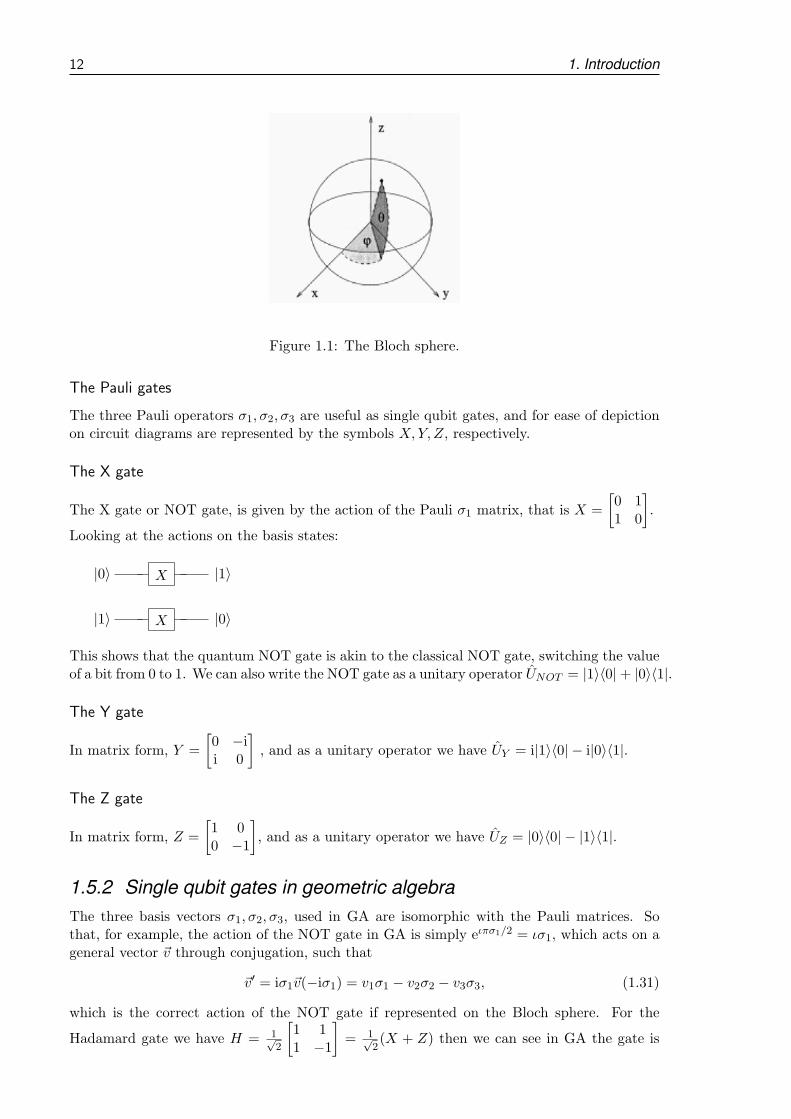
12 1. Introduction
Figure 1.1: The Bloch sphere.
The Pauli gates
The three Pauli operators σ1, σ2, σ3 are useful as single qubit gates, and for ease of depictionon circuit diagrams are represented by the symbols X,Y, Z, respectively.
The X gate
The X gate or NOT gate, is given by the action of the Pauli σ1 matrix, that is X =
[0 11 0
]
.
Looking at the actions on the basis states:
X|0〉 |1〉
X|1〉 |0〉
This shows that the quantum NOT gate is akin to the classical NOT gate, switching the valueof a bit from 0 to 1. We can also write the NOT gate as a unitary operator UNOT = |1〉〈0|+ |0〉〈1|.
The Y gate
In matrix form, Y =
[0 −ii 0
]
, and as a unitary operator we have UY = i|1〉〈0| − i|0〉〈1|.
The Z gate
In matrix form, Z =
[1 00 −1
]
, and as a unitary operator we have UZ = |0〉〈0| − |1〉〈1|.
1.5.2 Single qubit gates in geometric algebra
The three basis vectors σ1, σ2, σ3, used in GA are isomorphic with the Pauli matrices. Sothat, for example, the action of the NOT gate in GA is simply eιπσ1/2 = ισ1, which acts on ageneral vector ~v through conjugation, such that
~v′ = iσ1~v(−iσ1) = v1σ1 − v2σ2 − v3σ3, (1.31)
which is the correct action of the NOT gate if represented on the Bloch sphere. For the
Hadamard gate we have H = 1√2
[1 11 −1
]
= 1√2(X + Z) then we can see in GA the gate is

1.5 Quantum Gates 13
simply ι√2(σ1 + σ3). The T or π
8 gate can be written as
T =
[1 0
0 eiπ/4
]
≡ e−ιπσ3/8, (1.32)
which in this case is more obvious than the matrix form which has a π4 coefficient. Thus, GA
gives a simple and efficient representation for single qubit gates.
Java simulator
Single qubit gates - Hadamard gate
The action of the Hadamard gate is demonstrated in the Javasimulator. We can now see written alongside the gate a calcu-lation of how it transforms the |0〉 state into the 1√
2(|0〉+ |1〉)
state. At the bottom of the screen, we also see the behaviorof the probability amplitudes of the wave function before andafter the action of the Hadamard gate.

14 1. Introduction
1.5.3 Two qubit gates
A system of two quantum bits is a four-dimensional Hilbert space H4 = H2 ⊗H2, having anorthonormal basis |00〉, |01〉, |10〉, |11〉 . For a two qubit state we can then write
|ψ〉 = α00 |00〉+ α01 |01〉+ α10 |10〉+ α11 |11〉 , (1.33)
with the normalization condition∑
x∈0,12|αx|2 = 1, (1.34)
where 0, 12 represents a string of 0’s and 1’s of length 2.
Definition 1.5.1 A binary quantum gate is a unitary mapping H4 → H4.
The Controlled-NOT or CNOT gate
A two qubit version of the NOT gate is the Controlled-NOT or CNOT gate and is representedin circuits by:
e
u|A〉 |A〉
|B〉 |B A〉+f
The top line of the circuit is the control line for the gate, represented by the filled in circle.The open circle indicates the qubit that will be flipped if the control line is set to one. The|A〉 line on the control line continues through the CNOT gate unchanged, however, a phasecan be ‘kicked back’ from the other line. The |B〉 line is the data qubit line, which combineswith the first qubit and produces the target qubit. The notation |B ⊕A〉 represents additionmodulo 2 or the XOR gate. This is meaningfully defined here because the input states areassumed to be basis states represented as 0 or 1 in this case. The XOR operation is 1, if oneof the input bits is 1 and the other one is 0, otherwise the XOR operation gives zero.
Similarly to single qubits, two qubit gates can be represented by transformation matrices,see definition (1.5.1), specifically for the CNOT gate:
UCN =
1 0 0 00 1 0 00 0 0 10 0 1 0
. (1.35)
Thus,
ψ′ = UCNψ =
1 0 0 00 1 0 00 0 0 10 0 1 0
α00
α01
α10
α11
=
α00
α01
α11
α10
.
This can also be written as a unitary operator |00〉〈00|+ |01〉〈01|+ |11〉〈10|+ |10〉〈11|. Forexample, if |ψ〉 = |10〉 the CNOT produces the state |ψ〉 = |11〉.

1.5 Quantum Gates 15
Universality
We have now reached an important point in the development of quantum gates, because itcan be shown that any multiple qubit gate can be composed from just controlled-NOT andsingle qubit gates [NC02]. It is found that any k-qubit unitary operation can be simulatedwith O(4kk) such gates. Of course, the set of possible single qubit gates is infinite, becausethis is the set of all possible unitary transformations. Other combinations of gates can befound as a basis if we only require it to be universal in an approximate sense, for examplethe controlled-NOT, along with the Hadamard gate and the π/8 gate, can be considered auniversal set of gates in an approximate sense.
So, with these two types of gates (CNOT and single qubit), we now have all the gateswe need to develop any quantum algorithm. This theorem is the quantum equivalent of theuniversality of the NAND gate in classical computing.
Other useful two qubit gates
The swap gate is used to swap the position of two qubits given by the matrix
1 0 0 00 0 1 00 1 0 00 0 0 1
.
The Ctrl-Phase gate gate applies the phase gate operation if the control line is set,
Ctrl− phase =
1 0 0 00 1 0 00 0 1 00 0 0 eiφ
. If we set φ = π then we form the Ctrl− Z gate.
1.5.4 Three qubit gates
Three qubit gates are not required to develop a universal quantum computer but they areof theoretical interest. For example, the three qubit Toffoli gate can implement a reversibleNAND gate and the universality of the NAND gate in classical computing means we cantherefore duplicate any classical algorithm on a quantum computer.
The other property of classical computers is Fanout, which can also be implemented withthis gate, though only on basis states. Another process of classical computers is randomnumber generation and, because the Hadamard gate creates an equal superposition of twostates, upon measurement it gives a random choice of basis states, and so can be used tointroduce indeterminism into a quantum computer.
1.5.5 Measurements
Even though measurement is not a unitary transformation it can be useful in circuits, becauseit creates the operation of collapsing the quantum state to one of the basis values.
Given a state |ψ〉 = α |0〉+ β |1〉 a measurement is represented by:
where M represents the classical bits 0,1. Or for a 2 qubit state, given by (1.33), if we measure
the first qubit to be 0, we know we are left with the state: |ψ〉 = α00|00〉+α01|01〉√|α00|2+|α01|2
.

16 1. Introduction
1.6 General quantum circuits
The rows and columns of the unitary transforms are labeled from left to right and top tobottom as 00...0,00...1, to 11...1, with the bottom-most wire being the least significant bit. Awire carrying n qubits is represented by:
n
Quantum circuits must satisfy:
1. No loops: a loop or some sort of feedback would make the circuit non-reversible and sois not permitted. Also, the circuit would become non-linear.
2. No fan-in: in a classical circuit this is achieved by joining two wires together to form asingle wire (a bitwise or) but this operation is not reversible and therefore not unitaryand so not allowed.
3. No fan-out: it can be shown that quantum mechanics does not allow qubits to be copied,thus making general fan-out impossible. This result is also known as the no-cloningtheorem.
1.6.1 Copying circuit
The no-cloning theorem states that we cannot create a circuit to duplicate a general quantumstate, so it might appear that any form of copying is impossible, however we demonstrate thatwe can copy orthogonal states using the CNOT gate as shown below. The data qubit is passedstraight through, and the target qubit holds the result of the gate operation. If we set theinput target qubit to |0〉, then we can copy the set of orthogonal states |0〉 and |1〉 as shown.
e
u|0〉 |0〉
|0〉 0〉 e
u|1〉 |1〉
|0〉 1〉
So, in the two cases above, the data bit is copied.We can prove this algebraically, with a general basis state |ψxy〉 = |x, 0〉, where x ∈ 0, 1 andy = 0, we have for the final state
ψ′ = [CNOT ]
[[1− xx
]
⊗[10
]]
.
If we expand the tensor product and act with the CNOT gate we find
ψ′ =
1 0 0 00 1 0 00 0 0 10 0 1 0
1− x0x0
=
1− x00x
= (1− x)
1000
+ x
0001
,
which can be written conveniently in Dirac notation as
|ψ′〉 = (1− x)|0, 0〉+ x|1, 1〉).We notice this can be combined into a single term |ψ′〉 = |x, x〉, which implies we have themapping |x, 0〉 → |x, x〉, thus showing that we are successfully copying the input basis state|x〉, where x ∈ 0, 1.

1.6 General quantum circuits 17
1.6.2 Creating a Bell state or an EPR pair
The Bell state is a maximally entangled two qubit state, and is useful in modeling two-playergames, see Chapter 6. Consider the following circuit with 2 qubits:
e
uH|A〉
|B〉|ψ〉
Assuming |A〉 and |B〉 are basis states, we have an initial state |ψxy〉 = |x, y〉 where x, y ∈ 0, 1.We can construct the final state
ψ′ = [CNOT ]
[
[H]
[1− xx
]
⊗[1− yy
]]
.
Expanding the Hadamard gate and the tensor product:
ψ′ = [CNOT ]
[
1√2
[1
1− 2x
]
⊗[1− yy
]]
= [CNOT ] 1√2
1− yy
(1− 2x)(1− y)(1− 2x)y
.
Allowing the CNOT gate to act we obtain the final state
ψ′ =1√2
1 0 0 00 1 0 00 0 0 10 0 1 0
1− yy
(1− 2x)(1− y)(1− 2x)y
=
1√2
1− yy
(1− 2x)y(1− 2x)(1− y)
and writing as a sum of basis vectors
ψ′ =1− y√
2
1000
+
y√2
0100
+
(1− 2x)y√2
0010
+
(1− 2x)(1− y)√2
0001
.
This can be written conveniently as states: |ψ′〉 = 1√2(|0, y〉+ (−1)x|1, 1− y〉).
So, can we find a single unitary matrix applied to the input state in H4, such that
Ubell
(1− x)(1− y)(1− x)yx(1− y)xy
=
1√2
1− yy
(1− 2x)y(1− 2x)(1− y)
?
With some simple algebra, looking at the four possible input states, we find
Ubell =1√2
1 0 1 00 1 0 10 1 0 −11 0 −1 0
,
where we can fairly easily see that Ubell is unitary.
So, we can find ψ′ = Ubellψ, which can be used to switch to the Bell basis.

18 1. Introduction
Entanglement
Definition 1.6.1 A state z ∈ H4 of a two-qubit system is decomposable if z can be written as
a product of states in H2, z = x⊗ y. A state that is not decomposable is entangled.
So, for the Bell state, we require|00〉+ |11〉√
2= (a0|0〉+ a1|1〉)(b0|0〉+ b1|1〉) = a0b0|00〉+ a0b1|01〉+ a1b0|10〉+ a1b1|11〉 (1.36)
for some complex numbers a0, a1, b0, b1 ∈ C. However a0b0 =1√2, a0b1 = 0, a1b0 = 0 and
a1b1 =1√2, which is impossible, and so the state is entangled. It has been shown that correla-
tions as strong as entanglement cannot exist in classical physics, and it is one of the resourcesavailable to quantum computers unavailable on classical machines.
Given a general two qubit state
|ψ〉 = a|00〉+ b|01〉+ c|10〉+ d|11〉,
if it is not entangled, then we can split the state into two qubits, that is |ψ〉 = |φ〉|χ〉. Ifall four terms are present, then to be able to factorize the state we must have b/a = d/c orad− bc = 0. Hence, ad− bc = 0 implies no entanglement.
1.6.3 Quantum parallelism
Because of the property of the superposition of states, a quantum computer can be constructedto be massively parallel, for example, a quantum computer can evaluate a function f(x) formany different values of x simultaneously. Suppose we have a function from a binary state toa binary state f(x) : 0, 1→ 0, 1 . This can be conveniently computed with a 2 qubit quantumcomputer using the unitary transformation
|x, y〉 Uf−→ |x, y ⊕ f(x)〉 .
We know that given, say, a classical circuit for computing f(x), we can always mimic it witha quantum circuit of comparable efficiency. So, we will call this black box circuit Uf .
This can be also represented as a unitary matrix:
Uf =
1− f(0) f(0) 0 0f(0) 1− f(0) 0 00 0 1− f(1) f(1)0 0 f(1) 1− f(1)
. (1.37)
The initial state |ψ〉 can be obtained by passing |0〉 through a Hadamard gate. Now, we cansee from the final state that a measurement on |φ〉 gives either |0, f(0)〉 or |1, f(1)〉 . So, ifthe first qubit measures the state |0〉, then the second qubit will be |f(0)〉, if the first qubit

1.7 Summary of quantum algorithms 19
measures |1〉 then the second qubit will be |f(1)〉. So, the final quantum state appears to haveevaluated the function f(x) for two different values of x simultaneously.
If we now had two data bits x1 and x2 instead of just x, and each initially passing throughHadamard gates, we would create an input state:
|ψ0〉 =|0〉+ |1〉√
2.|0〉+ |1〉√
2|0〉 = |00〉+ |01〉+ |10〉+ |11〉
2|0〉 . (1.38)
We can write H⊗2 to denote the action of two Hadamard gates on two qubits. Similarly for nHadamard gates acting on n qubits we can write H⊗n. For H⊗n acting on n |0〉 state qubitswe will obtain:
1√2n
∑
x∈0,1n|x〉 , (1.39)
which produces an equal superposition of all basis states. This equal superposition of the basisstates is in fact a convenient starting state for many algorithms.
We can now extend the concept to quantum parallel evaluation of a function with an nbit input x and 1 bit out, f(x), which can be performed in the following manner:
1. |0〉⊗n |0〉 : prepare an n+ 1 qubit state
2.H⊗n
−→ 1√2n
∑
x∈0,1n |x〉 |0〉 : apply Hadamard transformation
3.Uf−→ 1√
2n
∑
x∈0,1n |x〉 |f(x)〉 : apply Uf
4.M−→ (x, f(x)) : measure the state.
So, all possible values of f are available even though we only evaluated the algorithm once.However, measurement of the final state only gives f(x) for a single value of x at a time.We could fairly straightforwardly extend the function f(x) to output several bits, that isf(x) : 0, 1n → 0, 1m where m,n ∈ Z
+.Even though the function has been evaluated at several values of x simultaneously and is
held in the quantum qubits, we have no way of accessing this information, because after a singlemeasurement the wave function collapses and we lose all other amplitudes. We need some wayto extract the extra information, in order to take full advantage of quantum parallelism. Thisis implemented in Grover’s algorithm where a black box oracle is used and the results ofmany parallel operations are interfered with each other to allow a measurement to return thesolution state.
1.7 Summary of quantum algorithms
Currently, two main classes of problems are known, where it appears a quantum computerwill outperform a classical one. Firstly, Shor’s quantum algorithm which factorizes largenumbers exponentially faster than a classical computer and which is based on the quantumFourier transform. Classically, the Fourier transform takes roughly N log(N) = n2n steps totransform N = 2n numbers, whereas a quantum computer takes about log2(N) = n2 steps, anexponential saving. The second main class of quantum algorithms, allowing a speedup overclassical computers although not an exponential speedup, is the quantum search algorithms.Given a search space of size N , and no prior knowledge of its structure, we want to findan element satisfying a known property. Classically, this problem requires N operations,but the quantum search algorithm allows it to be solved in
√N operations. Combining
these two algorithms, we find the quantum counting algorithm which can count the number
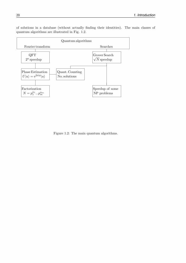
20 1. Introduction
of solutions in a database (without actually finding their identities). The main classes ofquantum algorithms are illustrated in Fig. 1.2.
Quantumalgorithms
Fourier transform Searches
Grover Search√N speedup
QFT
2n speedup
PhaseEstimation
U |u〉 = e2πiφ|u〉Quant.Counting
No. solutions
Factorization
N = pα11 ...pαm
m
Speedup of some
NP problems
Figure 1.2: The main quantum algorithms.

2
The Fourier Transform and the Phase
Estimation Algorithm
Initially, we describe the quantum Fourier transform (QFT) followed by a review of the phaseestimation algorithm which is based on the QFT. This algorithm is important because itforms the basis for Shor’s factorization algorithm which provides an exponential speedup overequivalent classical algorithms. This investigation firstly produces a new result of an exacterror formula for the phase estimation algorithm and secondly we develop, in the followingchapter, an alternative approach to the Grover search process using the phase estimationprocedure.
2.1 Quantum Fourier transform (QFT)
2.1.1 Definition of the Fourier transform
The discrete Fourier transform (DFT), takes as input a vector of N complex numbers,x0, . . . , xN−1 and outputs the transformed data as a vector of complex numbers y0, . . . , yN−1
defined by
yk =1√N
N−1∑
j=0
xje2πijk/N . (2.1)
The quantum Fourier transform acting on a set of basis states |0〉, . . . , |N − 1〉 is defined tobe a linear operator with the following action on an arbitrary state:
N−1∑
j=0
xj |j〉 →N−1∑
k=0
yk|k〉. (2.2)
We, of course, can presume that the initial state is normalized to one, that is:
N−1∑
j=0
x∗jxj =N−1∑
j=0
|xj |2 = 1.
So, for the transformed state we have:
N−1∑
k=0
|yk|2 =N−1∑
k=0
1
N
N−1∑
j=0
x∗je−2πijk/Nxje
2πijk/N =N−1∑
k=0
1
N=N
N= 1.
So, we can see that the Fourier transform acting on a general state is unitary, and thus canbe implemented as the dynamics for a quantum computer.
2.1.2 Definition of binary expansion
In the following analysis we takeN = 2n , where n is some integer and the basis |0〉, . . . , |2n − 1〉is the computational basis for an n qubit quantum computer. We will also represent the state|j〉n or |j〉⊗n using a binary expansion written as j = j1j2 . . . jn, where
j = j12n−1 + j22
n−2 + ...+ jn20. (2.3)
22 2. The Fourier Transform and the Phase Estimation Algorithm
We will also use the notation 0.jℓjℓ+1 . . . jn to represent a related binary fraction. That is, ifwe divide Eq. (2.3) by 2k and we find the fractional part
frac
(j
2k
)
= jℓ/2 + jℓ+1/22 + ...+ jn/2
k = 0.jℓjℓ+1 . . . jn =
n∑
i=ℓ
ji/2i, (2.4)
where ℓ = n+ 1− k, then we will find typically that we can drop the integer part of manyexpressions because when we find terms such ei2πj , obviously any integer part will contributean extra 2π, and so will not affect its numerical value.
2.1.3 Rearranging the Fourier transform formula
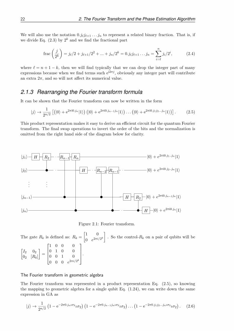
It can be shown that the Fourier transform can now be written in the form
|j〉 → 1
2n/2[(|0〉+ e2πi0.jn |1〉
) (|0〉+ e2πi0.jn−1jn |1〉
). . .(|0〉+ e2πi0.j1j2...jn |1〉
)]. (2.5)
This product representation makes it easy to derive an efficient circuit for the quantum Fouriertransform. The final swap operations to invert the order of the bits and the normalization isomitted from the right hand side of the diagram below for clarity.
H R2 Rn−1 Rn
u
u
u
|j1〉 |0〉+ e2πi0.j1..jn |1〉
H Rn−2 Rn−1
u
u
|j2〉 |0〉+ e2πi0.j2..jn |1〉
.
.
....
H R2
u
|jn−1〉 |0〉+ e2πi0.jn−1jn |1〉
H|jn〉 |0〉+ e2πi0.jn |1〉
Figure 2.1: Fourier transform.
The gate Rk is defined as: Rk =
[1 0
0 e2πi/2k
]
. So the control-Rk on a pair of qubits will be
[I2 0202 [Rk]
]
=
1 0 0 00 1 0 00 0 1 0
0 0 0 e2πi/2k
.
The Fourier transform in geometric algebra
The Fourier transform was represented in a product representation Eq. (2.5), so knowingthe mapping to geometric algebra for a single qubit Eq. (1.24), we can write down the sameexpression in GA as
|j〉 → 1
2n/2(1− e−2π0.jnισ3ισ2
) (1− e−2π0.jn−1jnισ3ισ2
). . .(1− e−2π0.j1j2...jnισ3ισ2
). (2.6)

2.2 Phase estimation 23
2.2 Phase estimation
The Fourier transform is the key to the phase estimation algorithm, which is the eigenvaluedetermination of a unitary matrix. That is we have:
U |u〉 = e2πiφ|u〉. (2.7)
Suppose a unitary operator U has an eigenvector |u〉 with eigenvalue e2πiφ, where the value ofφ ∈ ℜ is unknown. The goal of the phase estimation algorithm is to estimate φ. To performthe estimation, we assume that we have available black boxes, sometimes known as oracles,capable of performing the controlled-U2j operation, for selected non-negative integers j.
U2j |u〉 = U . . . U︸ ︷︷ ︸
2j terms
|u〉 = e2πi(2jφ)|u〉 (2.8)
The algorithm uses two registers. The first register contains t qubits initially in the state |0〉.How we choose t depends on two things, the number of digits of accuracy we wish to havein our estimate of φ, and with what probability we wish the phase estimation procedure tobe successful. The second register begins in the state |u〉 and contains as many qubits asnecessary to store |u〉. Phase estimation is performed in two stages. The first stage is shownbelow, where we have omitted the normalization for simplicity.
H
u
|0〉 |0〉+ e2πi(2t−1φ)|1〉
H
u
|0〉 |0〉+ e2πi(2t−2φ)|1〉
First register t qubits
.
.
.
....
H
u
|0〉 |0〉+ e2πi(21φ)|1〉
H
u
|0〉 |0〉+ e2πi(20φ)|1〉
U20 U21 U2t−2U2t−1|u〉 |u〉
Second register
Figure 2.2: Phase Estimation.
This circuit begins by applying a Hadamard transform to the first register, followed byapplication of controlled-U operations on the second register, with U raised to successivepowers of two. The final stage of the first register is seen to be therefore
1
2t/2
(
|0〉+ e2πi2t−1φ|1〉
)(
|0〉+ e2πi2t−2φ|1〉
)
. . .(
|0〉+ e2πi20φ|1〉
)
(2.9)
and by multiplying out the brackets, this can be seen to equal
1
2t/2
2t−1∑
k=0
e2πiφk|k〉. (2.10)

24 2. The Fourier Transform and the Phase Estimation Algorithm
We omit a description of the second register because it stays in the state |u〉 throughout thecomputation. We can describe the transformation by:
(If ⊗ U j
)(|t〉 ⊗ |u〉) = |t〉 ⊗ U j |u〉 = e2πijφ|t〉|u〉. (2.11)
Suppose now that φ can be expressed exactly in t bits, as φ = 0.φ1φ2 . . . φt, then the firstregister can be written:
1
2n/2
(
|0〉+ e2πi0.φn |1〉)(
|0〉+ e2πi0.φn−1φn |1〉)
. . .(
|0〉+ e2πi0.φ1φ2...φn |1〉)
. (2.12)
Comparing with (2.5), we see this is exactly the QFT of the state |φ1φ2 . . . φn〉. So, applyingthe inverse quantum Fourier transform to the first register will give us φ. That is
1
2t/2
2t−1∑
j=0
e2πiφj |j〉|u〉 F†=⇒ |φ〉|u〉. (2.13)
So, a measurement on the first register in the computational basis gives us φ exactly (assumingit can be exactly represented in the available t qubits).
2.3 Reliability of Estimate
Generally speaking, the phase φ may not be representable in a fraction containing n terms andso only an approximation will typically be obtained. However, if we choose t ≥ n qubits in thefirst register, we obtain φ accurate to n qubits with probability of success = 1− ǫ. Currently,only approximate formulas are known for this relationship, such as the one given by Nielsenand Chuang:
t− n ≤⌈
log2
(1
2ǫ+
1
2
)⌉
. (2.14)
However, this approximate formula was found to lack usefulness when actual simulations werecarried out because it was desired to compare actual errors obtained with a reliable estimate,so that convergence to an exact answer could be observed. Because of this, we now derive anexact formula for the maximum roundoff error from first principles.
If the phase φ, used in phase estimation, cannot be expressed exactly in t bits, then thealgorithm will only form an estimate for the value of φ. However, to calculate φ accurate ton bits with probability of success 1− ǫ, we need to find a t = t(n, ǫ). An exact formula wasobtained using p = t− n as:
ǫmax =2
π2ψ′(1 + 2p
2
)
, (2.15)
where ψ′(z) = dψdz is the trigamma function, ψ(z) = Γ′(z)
Γ(z) is the digamma function and Γ(z) =∫∞0 tz−1e−tdt is the standard gamma function.
We have written ǫmax, because for a complete range of possible φ angles, this will be theworst possible error. So, if we run the phase estimation procedure many times with randomvalues of φ, the worst error will converge to ǫmax.
Expressions are also developed in the limit as the number of qubits t → ∞ and in thelimit as the added qubits p→∞. The exact formula is useful in confirming classical programssimulating quantum phase estimation.
2.3.1 Introduction
Phase estimation is an integral part of Shor’s algorithm [Sho97], so an exact expression forthe maximum probability of error is valuable in order to precisely achieve a predeterminedaccuracy.

2.3 Reliability of Estimate 25
Given the eigenvalue equation U |u〉 = e2πiφ|u〉 for a unitary operator U , we can find anapproximation to the phase φ ∈ [0, 1) using the quantum phase estimation procedure [Mos99].The first stage in phase estimation produces, in the measurement register with a t qubit basis|k〉, the state [NC02]
|φ〉Stage1 =1
2t/2
2t−1∑
k=0
e2πiφk |k〉. (2.16)
If φ = b/2t for some integer b = 0, 1 , . . . 2t − 1, then
|φ〉Stage1 =2t−1∑
k=0
yk|k〉 , with yk =e2πibk/2
t
2t/2(2.17)
is the discrete Fourier transform of the basis state |b〉, that is, the state with amplitudesxk = δkb. We then read off the exact phase φ = b/2t, from the inverse Fourier transform, as|b〉 = F†|φ〉.
In general, however, when φ cannot be written in an exact t bit binary expansion, theinverse Fourier transform, in the final stage of the phase estimation procedure, yields a state
|φ〉 ≡ F†|φ〉Stage1 , (2.18)
from which we only obtain an estimate for φ. That is, the coefficients xk of the state |φ〉 inthe t qubit basis |k〉, will yield probabilities which peak at the values of k closest to φ.
Given a desired accuracy s with an associated probability of success 1− ǫ, however, we candetermine the number of extra qubits p necessary to be added to the register for φ. Previously,Cleve, Ekert, Macchiavello and Mosca [CEMM98] determined the following upper bound:
p ≤ pCEM =
⌈
log2
(1
2ǫ+
1
2
)⌉
. (2.19)
A similar derivation is given in Nielsen and Chuang [NC02] using similar approximations (forexample the derivation of equation 5.28). More recently in [IB02] another upper bound wasdeveloped which also still used approximations.
Our goal now is to derive an upper bound which avoids the approximations used in theabove formulas and, hence, obtain a precise result.
2.3.2 Accuracy formula
Initially we follow the procedure given in [CEMM98]. Let b be the integer in the range 0 to2t − 1 such that b/2t = 0.b1 . . . bt is the best t bit approximation to φ, which is less than φ,then we define
δ = φ− b/2t,which is the difference between φ and b/2t and where clearly 0 ≤ δ < 2−t. The first stage ofthe phase estimation procedure produces the state given by Eq. (2.16). Applying the inversequantum Fourier transform to this state produces
|φ〉 =2t−1∑
k=0
xk |k〉 , (2.20)
where
xk =1
2t
2t−1∑
ℓ=0
e2πi(φ−k/2t)ℓ =
1
2t1− e2πi 2
tδ
1− e2πi(δ−k−b2t
). (2.21)
Assuming the outcome of the final measurement is m, we can bound the probability of obtain-ing a value of m such that |m− b| ≤ e, where e is a positive integer characterizing our desired

26 2. The Fourier Transform and the Phase Estimation Algorithm
tolerance to error and where m and b are integers such that 0 ≤ m < 2t and 0 ≤ b < 2t. Theprobability of observing such an m is given by
p(|m− b| ≤ e) =e∑
ℓ=−e|xb+ℓ|2 (2.22)
which is simply the sum of the probabilities of the states within e of b, where
xb+ℓ =1
2t1− e2πi 2
tδ
1− e2πi(δ−ℓ/2t), (2.23)
which is the standard result obtained from Eq. (2.21), (in particular see equation 5.26 in[NC02]). Typically, at this point approximations are now made to simplify xℓ, however, weproceed without approximations. We have
|xb+ℓ|2 =1
22t1− cos(2π2tδ)
1− cos(2π(δ − ℓ/2t)) . (2.24)
If we wish to approximate φ to an accuracy of 2−s, we choose e = 2t−s−1 = 2p−1 1, usingt = s+ p, and if we denote the probability of failure
ǫ = p(|m− b| > e), (2.25)
then we have
ǫ = 1− 1− cos 2π2tδ
22t
2p−1∑
ℓ=−2p−1
1
1− cos 2π(δ − ℓ/2t) . (2.26)
This formula assumes that for a measurement m, we have a successful result if we measure astate either side of b within a distance of e, which is the conventional assumption.
This definition of error, however, is asymmetric because there will be unequal numbers ofstates summed about the phase angle φ in order to give the probability of a successful result,because an odd number of states is being summed. We now present a definition of the errorwhich is symmetric about φ.
Modified definition of error
Given an actual angle φ that we are seeking to approximate in the phase estimation procedure,a measurement is called successful if it lies within a certain tolerance e of the true value φ.That is, for a measurement of state m out of a possible 2t states, the probability of failure willbe
ǫ = p
(∣∣∣2π
m
2t− φ
∣∣∣ >
1
2
2π
2s
)
. (2.27)
Thus, we consider the angle to be successfully measured accurate to s bits, if the estimated φlies in the range φ± 1
22π2s . Considering our previous definition Eq. (2.25), due to the fact that
b is defined to be always less than φ, then compared to the previous definition of ǫ, we losethe outermost state at the lower end of the summation in Eq. (2.26) as shown in Fig. (2.3).For example, for p = 1, the upper bracket in Fig. (2.3) (representing the error bound) canonly cover two states instead of three, and so the sum in Eq. (2.26) will now sum from 0 to 1,instead of −1 to 1, for this case.
1Nielsen and Chuang [NC02] in the preliminary to Eq. 5.35, appear to have written incorrectly 2p−1 instead
of 2p−1.

2.3 Reliability of Estimate 27
An optimal bound
Based on this new definition then for all cases we need to add 1 to the lower end of thesummation giving
ǫ = 1− 1− cos 2π2tδ
22t
2p−1∑
ℓ=−2p−1+1
1
1− cos 2π(δ − ℓ/2t) (2.28)
and if we define a = 2tδ and rearrange the cosine term in the summation, we find
ǫ = 1− 1− cos 2πa
22t+1
2p−1∑
ℓ=−2p−1+1
csc2π
2t(a− ℓ). (2.29)
6
p = 1 ,∑1
0
︷︸︸︷0 1
︷︸︸︷
p = 2 ,∑2
−1
−101 2
︷︸︸︷
p = 3 ,∑4
−3
−20 2 4
Limits of summation, Eq. (2.28)
Figure 2.3: Analysis of phase estimation accuracy.
Next, we demonstrate that the right hand side of Eq. (2.29) takes its maximum value ata = 1
2 . Since we know 0 ≤ a < 1, and since we expect the maximum value of ǫ = ǫ(a, t, p)to lie about midway between the two nearest states to generate the largest error, that is ata = 1/2, we will substitute a = 1
2 +∆, where ∆≪ 12 . To maximize ǫ we need to minimize
cos 2π
(1
2+ ∆
) 2p−1∑
ℓ=−2p−1+1
csc2π
2t
(1
2− ℓ+∆
)
, (2.30)
as a function of ∆. Expanding to quadratic order with a Taylor series, we seek to minimize(1− π2∆2 +O(∆4)
) (c0 + c1∆+ c2∆
2 + c3∆3 +O(∆4)
), (2.31)
where ci are the coefficients of the Taylor expansion of cosecant2 in ∆. We find by the oddsymmetry of the cotangent about ℓ = 1
2 that
c1 =2π
2t
2p−1∑
ℓ=−2p−1+1
cotπ
2t(1
2− ℓ) csc2 π
2t(1
2− ℓ) = 0, (2.32)
and so we just need to minimize
c0 + (c2 − c0π2)∆2 +O(∆3). (2.33)
Differentiating, we see we have an extremum at ∆ = 0 and, therefore, ǫ(a, t, p) has a maximumat a = 1/2. Substituting a = 1
2 we obtain
ǫ ≤ 1− 2
22t
2p−1∑
ℓ=−2p−1+1
1
1− cos 2π2t (
12 − ℓ)
. (2.34)

28 2. The Fourier Transform and the Phase Estimation Algorithm
We note that the summation is symmetrical about ℓ = 1/2, and substituting t = p + s, weobtain for our final result
ǫ(s, p) = 1− 1
22(p+s)−2
2p−1∑
ℓ=1
1
1− cos π(2ℓ−1)
2(p+s)
. (2.35)
That is, given a desired accuracy of s bits, then if we add p more bits, we have a probabilityof success given by 1− ǫ, of obtaining a measurement to at least s bits of accuracy. Thus, wehave succeeded in deriving a best possible bound for the failure rate ǫ = ǫ(s, p).
2.3.3 Special cases
Numerical calculations show that ǫ(t, p) quickly approaches its asymptotic value as t → ∞,and this limit gives a fairly accurate upper bound for ǫ, for t greater than about 10 qubits.Using cosx ≥ 1− x2
2 which is valid for all x, and is accurate for x = O(1/2t) as t→∞
ǫ ≤ 1− 4
22t
2p−1∑
ℓ=1
1
1− (1− 12(
π2t (2ℓ− 1))2)
= 1− 8
π2
2p−1∑
ℓ=1
1
(2ℓ− 1)2. (2.36)
An exact form for this can be found in terms of the trigamma function, being a special caseof the polygamma function as shown in Abramowitz and Stegun [AS64], Eq. 6.4.5
ǫ ≤ 2
π2ψ′(1 + 2p
2
)
, (2.37)
where ψ′(z) = dψdz is the trigamma function, ψ(z) = Γ′(z)
Γ(z) is the digamma function and Γ(z) =∫∞0 tz−1e−tdt is the standard gamma function.
Now, considering the p→∞ limit, which also includes the t→∞ limit because t = p+ s,we can find an asymptotic form in the limit of large p also from [AS64], see Eq 6.4.12, namely
ǫ =4
π22−p, (2.38)
which shows that the error rate drops off exponentially with the extra qubits p. It is foundnumerically that the p =∞ limit is approached closely for small p, namely p ≈ 5. The formulaEq. (2.38) can be re-arranged to give
p∞ =
⌈
log22√2
π2ǫ
⌉
, (2.39)
which compares with the previous approximate formula shown in Eq. (2.19).
We have confirmed these formulas through a simulation by running the phase estimationalgorithm on the 2-dimensional rotation matrix, and undertaking a numerical search for therotation angle which maximizes the error ǫ. For the case p = 1 at the limit of large t usingEq. (2.36), we can calculate the maximum expected error to ǫ = 1− 8
π2 = 18.9430531%.
We can see from Table I, that even for a relatively small number of qubits such as t =s+ p = 15, the upper bound formula at t→∞ is accurate to seven decimal places.

2.3 Reliability of Estimate 29
s simulation ǫ(∞, 1) = 1− 8π2 ǫ(s, 1), Eq. (2.35)
1 14.013022 18.9430531 14.6446612 17.86115 18.9430531 17.8933053 18.680222 18.9430531 18.6821344 18.877800 18.9430531 18.8779185 18.926767 18.9430531 18.92677516 18.9389835 18.9430531 18.93898407 18.9420358 18.9430531 18.94203588 18.9427988 18.9430531 18.94279889 18.9429895 18.9430531 18.942989510 18.9430373 18.9430531 18.943037211 18.9430491 18.9430531 18.943049112 18.9430521 18.9430531 18.943052113 18.9430526 18.9430531 18.943052814 18.943052 18.9430531 18.9430530
Table 2.1: Simulation results, p = 1
ǫ % pEq.[2.37] pCEM p∞100.00 0 0 -118.943 1 2 19.937 2 3 25.040 3 4 32.530 4 5 41.266 5 6 50.632 6 7 60.3166 7 8 70.1583 8 9 80.07916 9 10 90.03958 10 11 100.019789 11 12 110.0098946 12 13 120.0049473 13 14 130.0024737 14 15 140.0012368 15 16 150.0006184 16 17 160.0003092 17 18 170.00015460 18 19 180.00007730 19 20 190.000038651 20 21 20
Table 2.2: Comparison of the t→∞ bounds formulas.
2.3.4 Summary
To calculate φ accurate to a specified s bits with a given probability of success 1− ǫ we addp extra qubits, where p is given by Eq. (2.35). If we have a large number of qubits, then wecan use the formula Eq. (2.37) valid at the t→∞ limit. In the p→∞ limit the asymptote isfound as a simple exponential form Eq. (2.38). We see that the previous upper bound formulapCEM overshoots by 1 for each choice of ǫ in Table II, so the newly derived formulas are asignificant improvement. We have found this formula to be useful in confirming the operationof classical algorithms, since it enables us to equate simulation outputs with exact numbers

30 2. The Fourier Transform and the Phase Estimation Algorithm
from Eq. (2.35).
The improved error formula in Eq. (2.35) was published in Public Library of Science,Volume 6(5). [JMCL11b] (attached).
Authors: J. M. Chappell(Adelaide University), M. A. Lohe(Adelaide University), Lorenzvon Smekal(Adelaide University), A. Iqbal(Adelaide University) and D. Abbott(Adelaide Uni-versity).
Statement of contributions: J. Chappell modified the conventional error formula by in-creasing its symmetry to allow an exact solution. J. Chappell, M. A. Lohe, Lorenz vonSmekal and A. Iqbal prepared the paper for publication, with checking by D. Abbott, M. A.Lohe and Lorenz von Smekal.
Signed:
J. M. Chappell Dr M.A. Lohe Dr L. von Smekal Dr A. Iqbal
Prof. D.Abbott

3
Grover’s Algorithm
Grover’s search algorithm [Gro98a] is a general search routine to retrieve a set of required itemsfrom an unstructured data set. Given an unsorted database of size N , we would classicallyexpect that it will take N/2 queries, on average, to find a specific entry, Grover’s quantumalgorithm, on the other hand, allows a specific entry to be found in just O(
√N) queries.
The speedup that this algorithm provides is a result of quantum parallelism. The databaseis effectively put into a uniform superposition of all possible search outcomes and then theresults interfered with each other to produce a probability distribution concentrated at thesolutions. In this section, after reviewing the Grover search procedure, we look at ways tospeedup the search and we find a different type of search based on the phase estimationprocedure, developed from the previous chapter (Chapter 2). We then proceed to model thesearch as the precession of a spin-12 particle. Generalizing the Hamiltonian based search, wefind SU(2) generators for the Grover search space, which can be modeled as the precession ofa single spin-12 particle. In the following chapter, because GA is known to be a very efficientformalism for handling rotations and hence precession, we extend this analysis using GA,which shows the efficiency of the formalism and also confirms the optimality of the standardGrover search [BBB+00], [Høy00].
3.1 Grover’s search algorithm
Suppose we have a search space of N elements, indexed by a number in the range 0 to N − 1.For convenience we assume N = 2n, so that the index can be stored in n bits. We assume wehave M solutions to the search query, with 1 ≤M ≤ N . A particular instance of the solutionset can be flagged by a function f , which takes as input an integer x in the range 0 to N − 1.We define f(x) = 1 if x is a solution to the search problem, and f(x) = 0 otherwise. Weassume we have an oracle which can recognize solutions to the search problem, defined as aunitary operator
|x〉|q〉 O−→ |x〉|q ⊕ f(x)〉, (3.1)
where | x〉 is the index register, ⊕ denotes addition modulo 2 and an extra bit called theoracle qubit |q〉 is a single qubit which is flipped if f(x) = 1, and is unchanged otherwise.For example we can check to see if x is a solution by preparing the state |x〉|0〉, applying theoracle, and checking to see if the oracle qubit has been flipped to |1〉. However, in practice, itis preferable to initialize the oracle qubit to (|0〉 − |1〉)/
√
(2), so that in this case the actionof the oracle will simply be to the flip the sign of the qubit, that is
|x〉 |0〉 − |1〉√2
O−→ (−1)f(x)|x〉 |0〉 − |1〉√2
. (3.2)
However, we notice in this case that the state of oracle qubit is not changed and so can beomitted from further analysis, hence the action of the oracle can now be written
|x〉 O−→ (−1)f(x)|x〉. (3.3)
We say that the oracle marks the solution to the search problem by shifting the phase of thesolution.
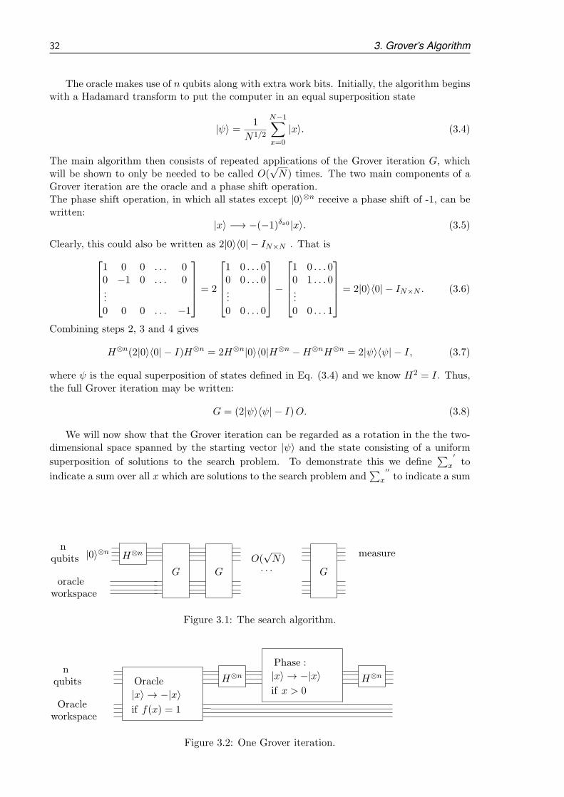
32 3. Grover’s Algorithm
The oracle makes use of n qubits along with extra work bits. Initially, the algorithm beginswith a Hadamard transform to put the computer in an equal superposition state
|ψ〉 = 1
N1/2
N−1∑
x=0
|x〉. (3.4)
The main algorithm then consists of repeated applications of the Grover iteration G, whichwill be shown to only be needed to be called O(
√N) times. The two main components of a
Grover iteration are the oracle and a phase shift operation.The phase shift operation, in which all states except |0〉⊗n receive a phase shift of -1, can bewritten:
|x〉 −→ −(−1)δx0 |x〉. (3.5)
Clearly, this could also be written as 2|0〉〈0| − IN×N . That is
1 0 0 . . . 00 −1 0 . . . 0...0 0 0 . . . −1
= 2
1 0 . . . 00 0 . . . 0...0 0 . . . 0
−
1 0 . . . 00 1 . . . 0...0 0 . . . 1
= 2|0〉〈0| − IN×N . (3.6)
Combining steps 2, 3 and 4 gives
H⊗n(2|0〉〈0| − I)H⊗n = 2H⊗n|0〉〈0|H⊗n −H⊗nH⊗n = 2|ψ〉〈ψ| − I, (3.7)
where ψ is the equal superposition of states defined in Eq. (3.4) and we know H2 = I. Thus,the full Grover iteration may be written:
G = (2|ψ〉〈ψ| − I)O. (3.8)
We will now show that the Grover iteration can be regarded as a rotation in the the two-dimensional space spanned by the starting vector |ψ〉 and the state consisting of a uniform
superposition of solutions to the search problem. To demonstrate this we define∑
x
′to
indicate a sum over all x which are solutions to the search problem and∑
x
′′to indicate a sum
G G G
H⊗n
oracleworkspace
nqubits |0〉
⊗n
. . .
measureO(√N)
Figure 3.1: The search algorithm.
Oracle
|x〉 → −|x〉if f(x) = 1
Phase :
|x〉 → −|x〉if x > 0
H⊗n H⊗n
Oracleworkspace
nqubits
Figure 3.2: One Grover iteration.

3.1 Grover’s search algorithm 33
over all x which are not solutions to the search problem. We can then define the normalizedstates
|m⊥〉 ≡ 1√N −M
∑
x
′′|x〉 (3.9)
|m〉 ≡ 1√M
∑
x
′|x〉.
It is then easy to see that
|ψ〉 =√
N −MN
|m⊥〉+√
M
N|m〉, (3.10)
and so the initial state |ψ〉 of the quantum computer is in the space spanned by |m⊥〉 and|m〉. Now, the effect of G operating on the state |ψ〉 can be seen as simply a rotation inthe plane of |m⊥〉 and |m〉. Referring to the Grover iteration defined in Eq.(3.8), initiallywe apply the oracle O. We have in the general case O(a|m⊥〉+ b|m〉) = a|m⊥〉 − b|m〉, so Ocreates a reflection about the vector |m⊥〉. Next, applying 2|ψ〉〈ψ| − I, we notice it also formsa reflection in the plane defined by |m⊥〉 and |m〉, about the vector |ψ〉 and the product oftwo reflections is a rotation. Thus, Gk|ψ〉 remains in the space defined by |m⊥〉 and |m〉 forall k. The angle of rotation is given by
cos θ/2 =√
(N −M)/N (3.11)
and clearly then also
sin θ/2 =√
M/N. (3.12)
Hence, we have |ψ〉 = cos θ2 |m⊥〉+ sin θ2 |m〉. Looking at Fig. 3.3 we can say
G|ψ〉 = cos3θ
2|m⊥〉+ sin
3θ
2|m〉, (3.13)
so this implies a rotation angle of θ.
Hence, it follows that the continued application of G takes the state to
Gk|ψ〉 = cos(2k + 1)θ
2|m⊥〉+ sin
(2k + 1)θ
2|m〉. (3.14)
Repeated applications of Grover’s iteration thus rotates the state vector by θ, closer andcloser to |m〉. When this occurs, an observation in the computational basis produces withhigh probability one of the outcomes superposed in |m〉, which is a solution to the searchproblem. Clearly, therefore, we could also write the Grover iteration in |m〉, |m⊥〉 space inmatrix form as
G =
[cos θ − sin θsin θ cos θ
]
. (3.15)
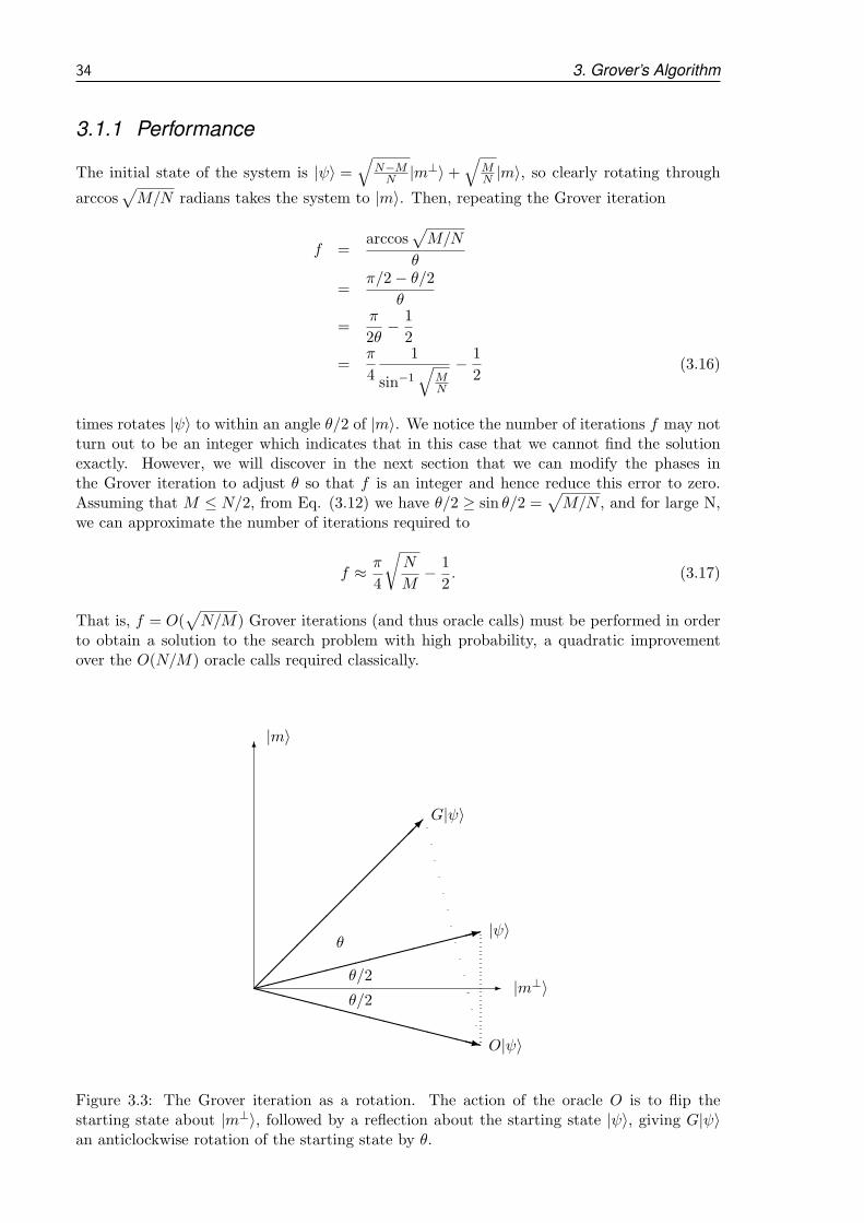
34 3. Grover’s Algorithm
3.1.1 Performance
The initial state of the system is |ψ〉 =√
N−MN |m⊥〉+
√MN |m〉, so clearly rotating through
arccos√
M/N radians takes the system to |m〉. Then, repeating the Grover iteration
f =arccos
√
M/N
θ
=π/2− θ/2
θ
=π
2θ− 1
2
=π
4
1
sin−1√
MN
− 1
2(3.16)
times rotates |ψ〉 to within an angle θ/2 of |m〉. We notice the number of iterations f may notturn out to be an integer which indicates that in this case that we cannot find the solutionexactly. However, we will discover in the next section that we can modify the phases inthe Grover iteration to adjust θ so that f is an integer and hence reduce this error to zero.Assuming that M ≤ N/2, from Eq. (3.12) we have θ/2 ≥ sin θ/2 =
√
M/N , and for large N,we can approximate the number of iterations required to
f ≈ π
4
√
N
M− 1
2. (3.17)
That is, f = O(√
N/M) Grover iterations (and thus oracle calls) must be performed in orderto obtain a solution to the search problem with high probability, a quadratic improvementover the O(N/M) oracle calls required classically.
-
6
:
XXXXXXXXXXXXXXXXz
|m〉
|m⊥〉
|ψ〉
O|ψ〉
G|ψ〉
θ
θ/2
θ/2
Figure 3.3: The Grover iteration as a rotation. The action of the oracle O is to flip thestarting state about |m⊥〉, followed by a reflection about the starting state |ψ〉, giving G|ψ〉an anticlockwise rotation of the starting state by θ.
3.1 Grover’s search algorithm 35
3.1.2 Quantum counting
It might appear from this result that any knowledge at all about the solution is going to requireO(√N) queries of the oracle, for example, to find out if even a solution exists. However, there is
a shortcut procedure called quantum counting, which applies the phase estimation procedureto the Grover iterate matrix directly, which in this case will return the eigenvalues of theGrover iterate matrix, from which we can calculate the number of solutions.
So, suppose |a〉 and |b〉 are the two eigenvectors of the Grover iteration in the space spannedby |m〉 and |m⊥〉 and let θ be the rotation angle determined by the Grover iteration. In thisspace the corresponding eigenvalues are eiθ and ei(2π−θ), seen clearly by inspecting the Groveriteration in matrix form Eq.(3.15).
The function of the phase estimation circuit is to estimate θ to s bits of accuracy, with aprobability of success at least 1 − ǫ. The first register contains t qubits to give the desiredaccuracy, as per the phase estimation algorithm and the second register contains n qubitssufficient to represent the database and to run the Grover iteration. The state of the secondregister is initialized to an equal superposition of all possible inputs
∑
x |x〉 by a Hadamardtransform, which can be shown to be an equal superposition of the the two eigenstates |a〉 and|b〉. So, phase estimation will give us an estimate of θ or 2π−θ accurate to within |∆θ| ≤ 2−s,with probability at least 1− ǫ. Quantum counting then uses the formula sin2 θ = M/N( Eq.(3.12)), and because we know N the size of the search space, we can calculate M , the numberof solutions.
However, once we know the number of solutions, by running the quantum counting al-gorithm, we now have redundant information, because we can now calculate the number ofiterations required either from quantum counting or from the Grover formula, found in Eq.(3.16). Writing out these two formulas we have
fgrover =π
4
1
sin−1(a)− 1
2, (3.18)
where a is the overlap amplitude of the starting wave function with the solution states andfrom quantum counting after finding θ, we can also find the number of iterations as
fqc =π
2θ− 1
2. (3.19)
Therefore, if we equate these two equations, we find
π
4
1
sin−1(a)− 1
2=
π
2θ− 1
2
1
2
1
sin−1(a)=
1
θ
2 sin−1(a) = θ.
From which we obtain the formula (which is related to Eq.(3.12))
a = sinθ
2. (3.20)
Hence, we can calculate the starting probability overlap amplitude, with the solution statefrom the measured θ obtained from phase estimation. Using Hadamard gates to generate thestarting probability distribution, this amplitude is fixed by the size of the search problem, if,however, we use a two-step starting probability distribution then, depending on which halfof the search space the solution lies in, we will obtain two different values of θ from phaseestimation.
For example using Hadamard gates to generate the initial probability distribution, we havea = 1/
√N . So, if we take N = 16 we have a = 1/4, and so fopt =
π4
1sin−1(1/4)
− 12 = 2.6083.
Using the phase estimation algorithm in the Java simulator with 7 qubits of accuracy weobtain fqc = 2.70± 0.135, which agrees within the uncertainty limits.

36 3. Grover’s Algorithm
3.1.3 Two-step starting probability distributions
-
6Probability amplitude
N
a1a2
1√N
Figure 3.4: Starting probability distribution. The first part of the Grover operator flips thestarting state |ψ〉 about the |m⊥〉 axis given by O|ψ〉, followed by a reflection about the startingstate axis |ψ〉, resulting in the state G|ψ〉, a rotation of the starting state by θ towards thesolution |m〉.
So, if we assume we have a two step probability distribution as shown in Fig. (3.4), thenlooking again at our previous result:
a = sinθ
2, (3.21)
we have 0 < θ < π/2, hence we have a 1:1 map between θ and a. For large databases, wehave a ∼
1√N→ 0 hence θ ≈ 2a. That is, the rotation angle for each Grover iteration is
approximately twice the probability amplitude at the solution state.If the solution lies in the left half of the probability distribution, then the angle corre-
sponding to this probability will be measured or 2 sin−1(a1), otherwise the angle θ based onthe other probability amplitude 2 sin−1(a2) will be measured. Hence, by running the phaseestimation procedure on the Grover matrix for the two level probability distribution, we candetermine which half of the search space the solution lies in. However, we could then repeatthis process on the half where the solution lies, partitioning this half into two parts, and thencontinuing the process until we are left with just one element in the search space, which mustbe the solution. So, if we have a search space of size N = 2n, then after n = logN applicationsof the phase estimation procedure, we will be left with a single entry and we will have thusfound the solution state. As an example a search space of size 64, will need to be split sixtimes (32,16,8,4,2,1) to reduce to a single entry which equals log2 64. The phase estimationprocedure requires O(log3(N)) operations, hence, overall, this search procedure will requireO(log4(N)) operations and therefore apparently exponentially faster then Grover’s algorithmof O(
√N).
The only change we have made to the phase estimation procedure is to include a two-stepprobability amplitude, which reduces one half of the probability distribution to zero andincreases the other half by the square root of two. So, in the phase estimation we will eithermeasure zero or θ = 2 sin−1(a). The two-step distribution is actually easily formed from auniform superposition of Hadamard gates with the first qubit left at zero, that is I⊗H⊗(n−1),which will replace the conventional H⊗n to form the uniform starting probability distribution.
This means the first half of the probability distribution will have amplitude√2√N
and the
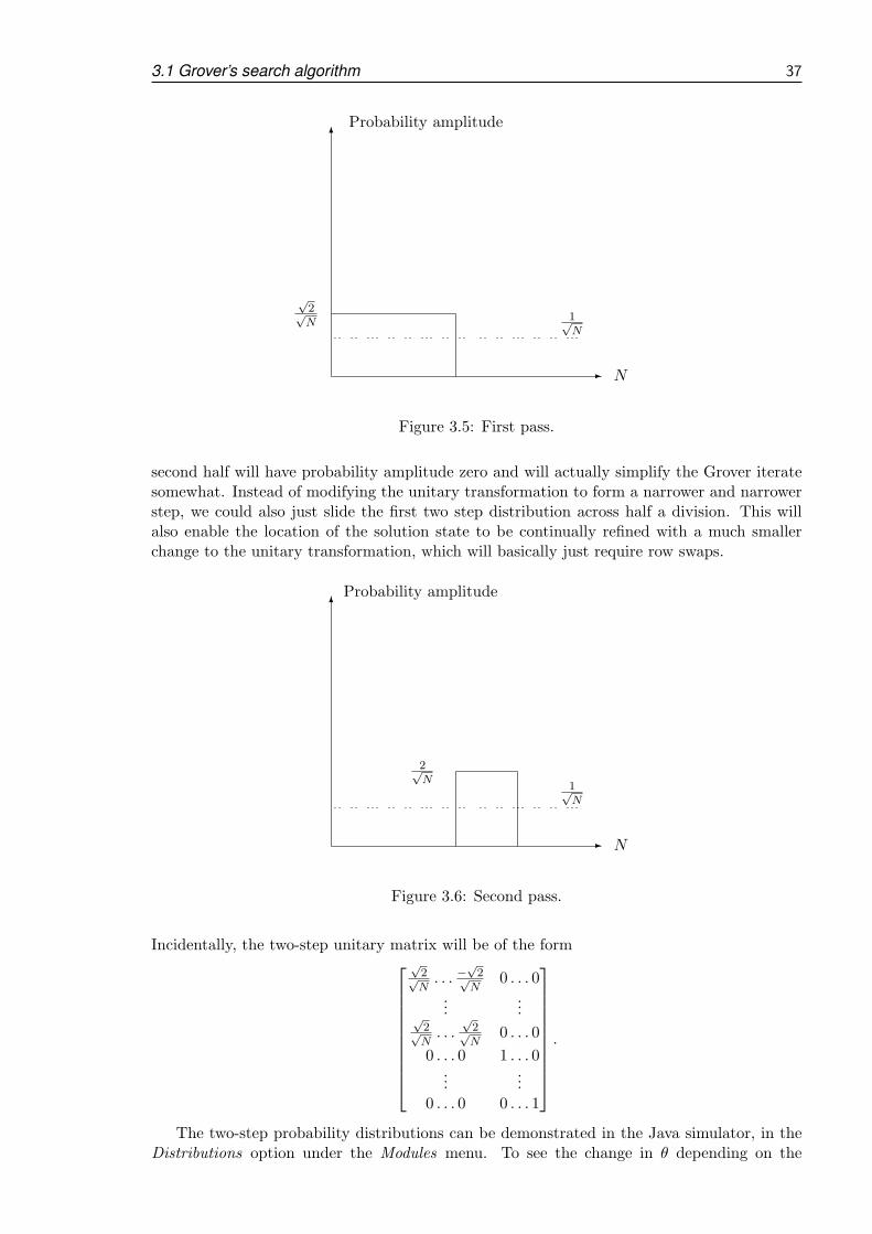
3.1 Grover’s search algorithm 37
-
6Probability amplitude
N
√2√N
1√N
Figure 3.5: First pass.
second half will have probability amplitude zero and will actually simplify the Grover iteratesomewhat. Instead of modifying the unitary transformation to form a narrower and narrowerstep, we could also just slide the first two step distribution across half a division. This willalso enable the location of the solution state to be continually refined with a much smallerchange to the unitary transformation, which will basically just require row swaps.
-
6Probability amplitude
N
2√N
1√N
Figure 3.6: Second pass.
Incidentally, the two-step unitary matrix will be of the form
√2√N. . . −
√2√N
0 . . . 0...
...√2√N. . .
√2√N
0 . . . 0
0 . . . 0 1 . . . 0...
...0 . . . 0 0 . . . 1
.
The two-step probability distributions can be demonstrated in the Java simulator, in theDistributions option under the Modules menu. To see the change in θ depending on the
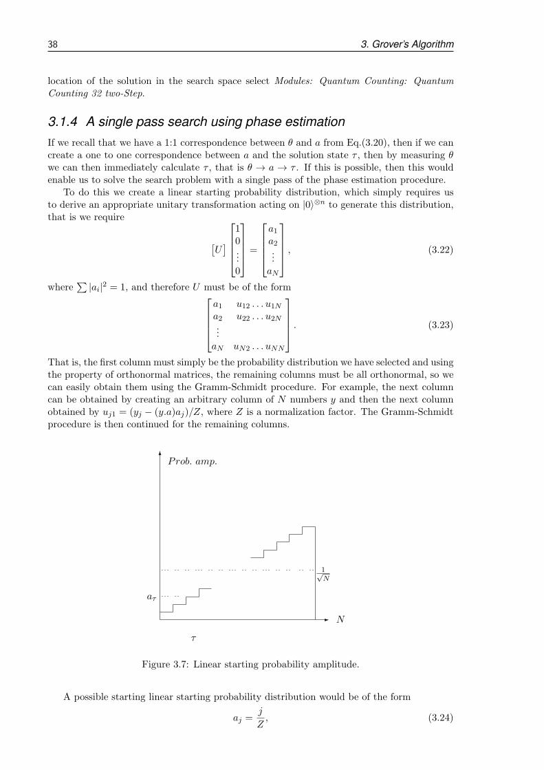
38 3. Grover’s Algorithm
location of the solution in the search space select Modules: Quantum Counting: Quantum
Counting 32 two-Step.
3.1.4 A single pass search using phase estimation
If we recall that we have a 1:1 correspondence between θ and a from Eq.(3.20), then if we cancreate a one to one correspondence between a and the solution state τ , then by measuring θwe can then immediately calculate τ , that is θ → a → τ . If this is possible, then this wouldenable us to solve the search problem with a single pass of the phase estimation procedure.
To do this we create a linear starting probability distribution, which simply requires usto derive an appropriate unitary transformation acting on |0〉⊗n to generate this distribution,that is we require
[U]
10...0
=
a1a2...aN
, (3.22)
where∑|ai|2 = 1, and therefore U must be of the form
a1 u12 . . . u1Na2 u22 . . . u2N...aN uN2 . . . uNN
. (3.23)
That is, the first column must simply be the probability distribution we have selected and usingthe property of orthonormal matrices, the remaining columns must be all orthonormal, so wecan easily obtain them using the Gramm-Schmidt procedure. For example, the next columncan be obtained by creating an arbitrary column of N numbers y and then the next columnobtained by uj1 = (yj − (y.a)aj)/Z, where Z is a normalization factor. The Gramm-Schmidtprocedure is then continued for the remaining columns.
-
6Prob. amp.
N
τ
aτ
1√N
Figure 3.7: Linear starting probability amplitude.
A possible starting linear starting probability distribution would be of the form
aj =j
Z, (3.24)

3.1 Grover’s search algorithm 39
where j = 0...N − 1 and the normalization factor Z would need to be defined as Z2 =N3
3 − N2
2 + N6 . We remember for large N that θ ≈ 2a = 2j
Z , therefore the angular distance weneed to be able to discriminate between successive states is
δθ =2(j + 1)
Z− 2j
Z=
2
Z. (3.25)
So, the error in the θ measurement 12s due to truncation of bits is δθ
2π and so using Eq. (3.25)we have
1
2s<
2/Z
2π,
which we can simplify to
2s > πZ (3.26)
s > logZ + log π (3.27)
but N3
3 > N3
3 − N2
2 + N6 , which approaches an equality for large N , so therefore we have
log
√
N3
3− N2
2+N
6+ log π < log
√
N3
3+ log π =
3
2logN + log
π√3<
3
2logN + 1
and N = 2n, hence, conservatively, we require
s >3
2logN + 1 =
3
2n+ 1. (3.28)
Hence, for a search space of size 16, that is n = 4, we require s = 7 bits in accuracy tomeasure θ sufficiently accurately to distinguish between adjacent states. Importantly, though,the number of bits required only scales as logN .
For the inverse Fourier transform we require O(t2) operations, however, we also require tctrl-Grover operations and to raise matrices to a power requires O(log2N) operations, whereN is the size of the search space. However, we need to repeat this procedure t−1 times, hencethis gives us O(log3N) operations.
If we have have multiple solutions, then the linear probability distribution method willfail because the phase estimation will return the angle based on the root mean square of thecontributing amplitudes, as discussed earlier, that is aeff =
√
a21 + a22 + ...+ a2m, and so thetarget solutions will be ambiguously defined. Fortunately, we can do a quantum countingprocedure with the standard Grover to confirm that there is only a single solution.
The circuit to calculate the eigenvalues of the Grover matrix given by
G|u〉 = e2πiθ|u〉, (3.29)
where u is an eigenvector and we have t qubits required for measurement.
From the phase estimation procedure, we obtain θ and inverting Eq.(3.20) and Eq.(3.24),we find the final result which enables us to calculate the solution state from the measured θ,from phase estimation:
τ = Z sinθ
2, (3.30)
where Z =√
N3
3 − N2
2 + N6 and we round τ to the nearest integer, which will be the index of
the solution state
τ = ⌈Z sinθ
2− 1
2⌉. (3.31)
Hence it appears possible to undertake a search process via an alternate process of using thephase estimation procedure on the Grover search matrix. This approach may have computa-tional advantages, however it will only be successful if there is a single target item within thesearch space.

40 3. Grover’s Algorithm
H
u
|0〉 |0〉+ e2πi(2t−1θ)|1〉
H
u
|0〉 |0〉+ e2πi(2t−2θ)|1〉
First register t qubits
.
.
.
....
H
u
|0〉 |0〉+ e2πi(21θ)|1〉
H
u
|0〉 |0〉+ e2πi(20θ)|1〉
G20 G21 G2t−2G2t−1|u〉 |u〉
Second register
Figure 3.8: Phase estimation of the Grover matrix
Java simulation
We can simulate a search over a database of 16 elements with, say, seven bits of precisionas shown in Table (3.1) by selecting Modules: Quantum Counting: Quantum Counting-16
U=Linear. We note that to achieve a result accurate to n qubits enabling us to calculate asolution with 81.1% reliability (18.9 % failure rate), we add one extra qubit. The matchingfirst and last columns in Table (3.1) indicate 100 percent reliability in finding the solution,using phase estimation.
3.2 Quantum search using a Hamiltonian
Following the discovery of the Grover search algorithm, which is designed to run in the circuitmodel form of quantum computing, Fenner [Fen00] discovered the equivalent Hamiltonian,which is a continuous time version of the Grover search [BK02a], [RC08]. This showed theequivalence between the two approaches and we also use the Hamiltonian form of the searchgiven here to find the SU(2) generators, as another alternative way to describe the Groversearch. The Hamiltonian form can also be run adiabatically [VDMV01], [EF02], [FGGS00],[RC02].
This type of search involves finding a Hamiltonian, which evolves the starting state, H|0〉onto the solution state |m〉. The Hamiltonian shown below achieves this and, in fact, can beshown to be equivalent to the standard Grover iteration G, if the Hamiltonian evolution isobserved at some constant time increment t0.
Assuming we have a search problem with exactly one solution, labeled m, we desire aHamiltonian H which when evolving over time changes some initial state, say |ψ0〉 into |m〉.As usual, we select our initial state |ψ0〉 to be |σ〉 = H|0〉. We use the Hamiltonian as shownin [Fen00]
H =2i√N
(|m〉〈σ| − |σ〉〈m|) , (3.32)
which can be shown for the appropriate time step t0, that e−iHt0 = G. We can, in fact, find
t0 =N(π−2 arccos 1√
N)
2√N−1
≈ 1. This shows that 1 time unit will equate to approximately 1 Grover

3.2 Quantum search using a Hamiltonian 41
τ a θ = 2 sin−1 a 7 bit τcalc =Z2 sin θ
2 − 12 τ ′ = ⌈τcalc − 1
2⌉0 0.0135 1.55 0 -0.5 01 0.0406 4.66 5.6 1.3 12 0.0677 7.76 8.4 2.2 23 0.0948 10.9 11.2 3.1 34 0.1218 14.0 14.0 4.0 45 0.1489 17.1 16.8 4.89 56 0.1760 20.3 19.6 5.79 67 0.2031 23.4 22.5 6.7 78 0.2302 26.6 25.3,28.1 7.59,8.47 89 0.2572 29.8 30.9 9.3 910 0.2843 33.0 33.7 10.2 1011 0.3114 36.3 36.5 11.1 1112 0.3385 39.6 39.3 11.92 1213 0.3655 42.9 42.1 12.8 1314 0.3926 46.2 45.0,47.8 13.6,14.46 1415 0.4197 49.6 50.6 15.28 15
Table 3.1: Phase estimation search simulation.
iteration in the circuit model. For analysis, we can restrict our analysis to the plane definedby |m〉 and |σ〉 as previously. Using |σ〉 = α|m〉+ β|y〉, in Eq. (3.32), we have
H =2i√N
(|m〉 (α〈m|+ β〈y|)− (α|m〉+ β|y〉) 〈m|) (3.33)
=2i√N
[0 β−β 0
]
=2iβ√NZX. (3.34)
So,
e−iHt = e−i( 2iβ√
NZX)t
= e2βt√NZX
.
We find
e2βt√NZX ≡ I + 2β√
NZXt+ (
2β√NZX)2t2/2! + (
2β√NZX)3t3/3! + . . .
but (ZX)2 = ZXZX = −ZXXZ = −I using [X,Z]+ = 0, so we find
e2βt√NZX
= I +2β√NtZX − (
2β√N
)2t2/2!− (2β√N
)3t3/3!ZX + . . .
hence
e2βt√NZX
= I cos2βt√N
+ ZX sin2βt√N
and so
e−iHt|σ〉 = cos2βt√N|σ〉+ sin
2βt√NZX|σ〉.
We note
ZX|σ〉 = ZX(α|m〉+ β|y〉) = β|m〉 − α|y〉.
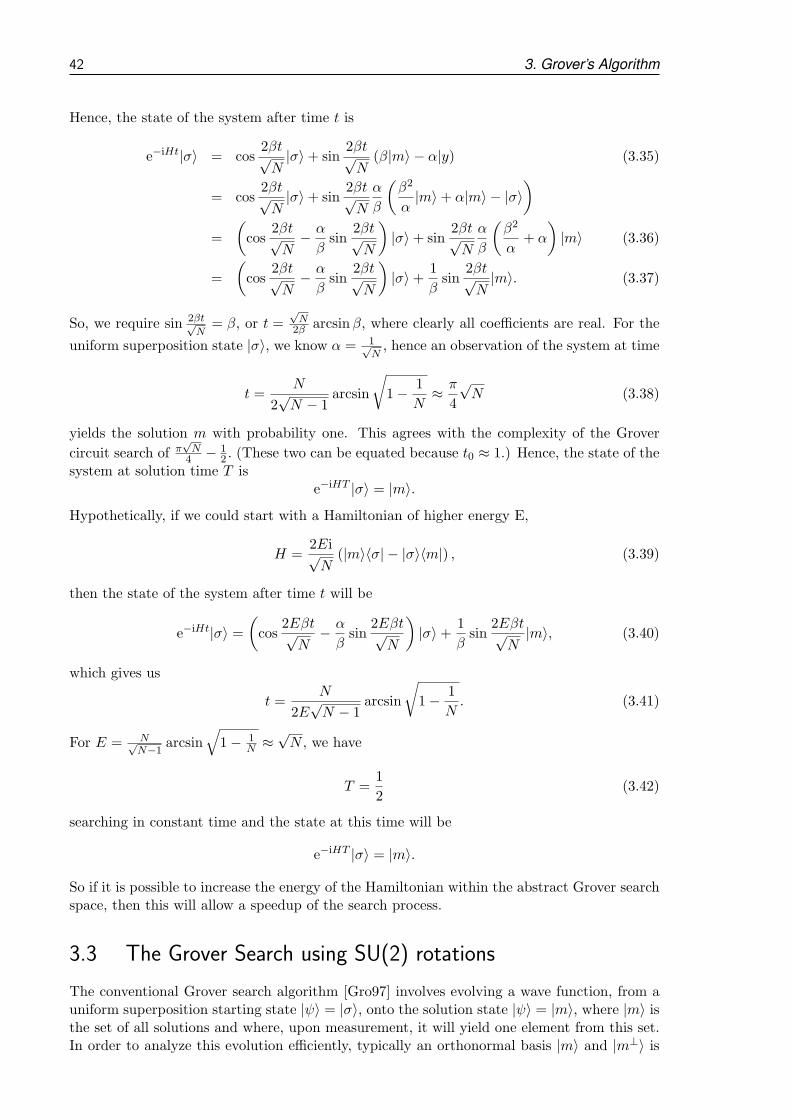
42 3. Grover’s Algorithm
Hence, the state of the system after time t is
e−iHt|σ〉 = cos2βt√N|σ〉+ sin
2βt√N
(β|m〉 − α|y) (3.35)
= cos2βt√N|σ〉+ sin
2βt√N
α
β
(β2
α|m〉+ α|m〉 − |σ〉
)
=
(
cos2βt√N− α
βsin
2βt√N
)
|σ〉+ sin2βt√N
α
β
(β2
α+ α
)
|m〉 (3.36)
=
(
cos2βt√N− α
βsin
2βt√N
)
|σ〉+ 1
βsin
2βt√N|m〉. (3.37)
So, we require sin 2βt√N
= β, or t =√N
2β arcsinβ, where clearly all coefficients are real. For the
uniform superposition state |σ〉, we know α = 1√N, hence an observation of the system at time
t =N
2√N − 1
arcsin
√
1− 1
N≈ π
4
√N (3.38)
yields the solution m with probability one. This agrees with the complexity of the Grover
circuit search of π√N
4 − 12 . (These two can be equated because t0 ≈ 1.) Hence, the state of the
system at solution time T ise−iHT |σ〉 = |m〉.
Hypothetically, if we could start with a Hamiltonian of higher energy E,
H =2Ei√N
(|m〉〈σ| − |σ〉〈m|) , (3.39)
then the state of the system after time t will be
e−iHt|σ〉 =(
cos2Eβt√N− α
βsin
2Eβt√N
)
|σ〉+ 1
βsin
2Eβt√N|m〉, (3.40)
which gives us
t =N
2E√N − 1
arcsin
√
1− 1
N. (3.41)
For E = N√N−1
arcsin√
1− 1N ≈
√N, we have
T =1
2(3.42)
searching in constant time and the state at this time will be
e−iHT |σ〉 = |m〉.
So if it is possible to increase the energy of the Hamiltonian within the abstract Grover searchspace, then this will allow a speedup of the search process.
3.3 The Grover Search using SU(2) rotations
The conventional Grover search algorithm [Gro97] involves evolving a wave function, from auniform superposition starting state |ψ〉 = |σ〉, onto the solution state |ψ〉 = |m〉, where |m〉 isthe set of all solutions and where, upon measurement, it will yield one element from this set.In order to analyze this evolution efficiently, typically an orthonormal basis |m〉 and |m⊥〉 is

3.3 The Grover Search using SU(2) rotations 43
defined, as shown on Fig. (3.9). We now identify an improved basis for analyzing the searchprocess, which allows a simple mapping to the Bloch sphere. From this, we are able to identifythe Grover search evolution as equivalent to the precession of the polarization axis of spin-12particle in a magnetic field, that is, precessing from the |σ〉 direction to the |m〉 direction.
In the field of adiabatic quantum computing [FG98a], it has been proposed that the Groversearch time can be reduced to unity [WY04], by simply increasing the energy of the searchHamiltonian, thus reducing the time. Using the precession analogy, this would be equivalent toincreasing the strength of the magnetic field, which would indeed reduce the precession time,thus appearing to speedup the search process. However, these ideas need to be reconciledwith proofs that Grover’s quantum search algorithm has been shown to be the optimal searchstrategy on a quantum computer [BBHT98], [Zal99], [SSB05], with complexity of O(
√N). We
will find that the answer to this dilemma lies in the oracle and, in fact, a circuit can indeedbe constructed to search in unit time provided the Oracle is enhanced. However as statedin [CvD10], there are still unresolved issues regarding the Hamiltonian search.
To analyze the Grover search algorithm, an SU(2) approach has been used previously[HL02], which found the conditions to find a search solution with a probability of one, whereaswith the conventional Grover operator, only an approximation to the solution state is everfound (except in the special case with just four states). An SO(3) picture has also beenemployed [LTL+01] to plot the path of the state vector during each application of the Groveroperator, which we will also find useful in plotting the path of the polarization axis in 3-space.
In this chapter, we will firstly define the three generators for the SU(2) search space. Fromthese, we can derive a general rotation in this search space and the standard Grover searchwill then be identified as simply a special case of this. We will show that raising the energy ofa search Hamiltonian in the adiabatic setting is equivalent to raising the Grover operator to apower in the circuit model representation and, as a by-product, we will give a formula for theGrover matrix raised to any non-integer power. The general search formula will also enableus to easily derive the phase matching condition for an exact search along with its matrixevolution. We will then use one of the generators to produce a quantum circuit for searchingin unit time, but which will require, unfortunately, an enhanced oracle in order to succeed.
3.3.1 The Grover search space
-
6
:
|m〉
|m⊥〉
α =√
MN
|σ〉
θ2
1
β =√1− α2
Figure 3.9: Geometry of starting state |σ〉. The starting state |σ〉 represented in the basis of|m〉 and |m⊥〉, with M solution states in a space of size N .
Our goal in the search procedure is to rotate the starting vector |σ〉 in the space spannedby |m〉 and |m⊥〉 onto the vector |m〉 so that, upon measurement, a solution to the search

44 3. Grover’s Algorithm
problem will be achieved.Grover’s solution to this involves iteratively applying an operator G defined by
G = − (I − 2|σ〉〈σ|) (I − 2|m〉〈m|) . (3.43)
This operator applied to the n = logN qubits representing the search space, rotates the statevector an angle θ at each application, with the number of iterations given by
R ≈ π
4
√
N
M. (3.44)
3.3.2 SU(2) generators for the Grover search space
Working from the two-dimensional complex space shown in Fig. (3.9), and restricting ourselvesto the well defined states |m〉 and |σ〉, we have four possible operators: |m〉〈σ|, |σ〉〈m|, |m〉〈m|and |σ〉〈σ|. From these we define
K = −β2
2P (3.45)
J1 =P − |σ〉〈σ| − |m〉〈m|
2|α|
J2 =−i (α∗|m〉〈σ| − α|σ〉〈m|)
2|α|β
J3 =|σ〉〈σ| − |m〉〈m|
2β,
where α = 〈σ|m〉, in general, a complex number, and β =√
1− |α|2. With
P =(|σ〉〈σ| − |m〉〈m|)2
β2, (3.46)
we find
[Ji, Jj ] = iǫijkJk (3.47)
[Ji, Jj ]+ = δijP
2[K, Ji] = 0,
confirming that we have an SU(2) algebra. Squaring the generators we find
J21 = J2
2 = J23 =
1
4β2(|σ〉〈σ| − |m〉〈m|)2 = 1
4P. (3.48)
We can easily check P |σ〉 = |σ〉 and P |m〉 = |m〉, with P 2 = P and the Casimir invariant
C = J21 + J2
2 + J23 =
3
4P,
which corresponds to a spin 12 system. We have raising and lowering operators
J± = J1 ± iJ2
and requiring
J+| ↑〉 = 0 (3.49)
J−| ↓〉 = 0,

3.3 The Grover Search using SU(2) rotations 45
we find the states of highest and lowest weight
| ↑〉 = secθ
2
(
sinθ
4|m〉 − eiδ cos
θ
4|σ〉)
| ↓〉 = secθ
2
(
cosθ
4|m〉 − eiδ sin
θ
4|σ〉)
,
which is a rotation of the |m〉 and |m⊥〉 axes by θ4 , where we have defined
sinθ
2= |α| (3.50)
and
α = |α|eiδ. (3.51)
We can then find
J3| ↑〉 = +1
2| ↑〉 (3.52)
J3| ↓〉 = −1
2| ↓〉,
as expected for a spin−12 system. Writing |σ〉 and |m〉 in this new basis, we obtain
|σ〉 = e−iδ
(
− cosθ
4| ↑〉+ sin
θ
4| ↓〉)
(3.53)
and
|m〉 = − sinθ
4| ↑〉+ cos
θ
4| ↓〉, (3.54)
with
|m⊥〉 = 1
β(|σ〉 − α∗|m〉) = cos
θ
4| ↑〉+ sin
θ
4| ↓〉. (3.55)
Using these results for |σ〉 and |m〉, and substituting into the Grover iteration Eq.(3.43), wefind
G = −I + 2 cos2θ
2| ↑〉〈↑ |+ sin θ| ↑〉〈↓ | − sin θ| ↓〉〈↑ |+ 2 cos2
θ
2| ↓〉〈↓ | (3.56)
and because we have an orthonormal basis for G, we can find a matrix form for the standardGrover iteration as
G =
[cos θ sin θ− sin θ cos θ
]
, (3.57)
where the starting state is
|σ〉 = e−iδ
[− cos θ4sin θ
4
]
. (3.58)
This matrix form can be used to calculate the Grover iterations, which can then be transformedback to the |σ〉, |m〉 basis when required. The matrix form for the exact Grover search isdeveloped in a later section.
General rotation
Applying a rotation ~φ = (φ1, φ2, φ3), where each φ1, φ2, φ3 apply to the generators J1, J2, J3respectively, so that we can define

46 3. Grover’s Algorithm
Q = e2i~φ. ~J (3.59)
= I + 2i~φ. ~J − |φ|2P
2!− |φ|
22~φ. ~J
3!+|φ|4P4!
. . .
= I + 2i~φ. ~J
|φ| sin |φ| − P (1− cos |φ|),
where we have used(2~φ. ~J
)2= 4
(φ21J
21 + φ22J
22 + φ23J
23
)= |φ|2P. (3.60)
Special case 1: ~φ = 0, φ2, 0In this case we are restricting ourselves to the generator, J2, so we have
Q2 = I + 2iJ2 sinφ2 − P (1− cosφ2)
and for φ2 = θ we findQ2|ψ〉 = G|ψ〉, (3.61)
that is, we have a direct relationship
e2iθJ2 |ψ〉 = G|ψ〉. (3.62)
Fenner [Fen00] found previously, as shown in section 5.2, that a Hamiltonian equivalent toJ2 up to a scale factor, can be equated to the standard Grover iteration, provided the wavefunction is measured at specified time intervals. This time step can simply be equated to θ andthe conventional Grover operator G is, therefore, just rotating an angle 2θ with the generatorJ2.
From this, we now investigate the possibility of raising G to any power, including non-integer powers.
Raising the Grover matrix to an arbitrary power
From the previous section, we can deduce the relationship
Gk|ψ〉 = e2ikθJ2 |ψ〉. (3.63)
= (I + 2iJ2 sin(kθ)− P (1− cos(kθ))) |ψ〉.
This formula which can be seen as a generalization of the Grover search iteration Gk for realk. We also see that raising the Grover operator to a power in this context is equivalent toincreasing the energy of the Hamiltonian, 2J2, [DKK03]. We have included the state |ψ〉because the equality applies to the effect of the operation on a particular state in the Groversubspace. To match the operators themselves, we would have
Gk = eikπe−2ki(π−θ)J2 . (3.64)
Of course, we know that Grover rotates the starting vector |σ〉, an angle π2− θ
2 onto the solutionstate, as shown in Fig.(3.9). Hence, a completed Grover search in a single operation will be
Q2 = e2i(π2− θ
2)J2 (3.65)
= I + 2iJ2 sin
(π
2− θ
2
)
− 4J22
(
1− cos
(π
2− θ
2
))
= I + 2iJ2 cosθ
2− P
(
1− sinθ
2
)
.

3.3 The Grover Search using SU(2) rotations 47
Incidentally, we can write this in terms of the Grover matrix as
Q2 =1 + 2α
2(1 + α)I +
1
4α(1 + α)G− 1 + 2α
4α(1 + α)G†, (3.66)
but the difficulty is to represent this as a circuit. To check this result, we multiply Q2 by thestarting state |σ〉, to find
Q2|σ〉 =α∗
|α| |m〉,
which is the solution as required up to a global phase.
Searching using J1
We know we can complete a search using J2, being equivalent to the standard Grover search,however, we can also complete a search using J1. In terms of J1, we have
Q1 = I + 2iJ1 sinφ− P (1− cosφ) . (3.67)
We find that the generator J1 rotates in the complex plane and so we need a rotation ofφ = −π
2 to complete the search, hence
Q1 = I − 2iJ1 − P (3.68)
= I − P(
1 +i
|α|
)
+ i|σ〉〈σ|+ |m〉〈m|
|α| .
In this case we find
Q1|σ〉 = i|m〉,
thus successfully completing the search. We notice that P commutes with the other operatorsso we can simplify the exponential, as follows:
e2ikθJ1 = eikθ(P−|σ〉〈σ|−|m〉〈m)/|α| (3.69)
= eikθ|α| e
− ikθ|α| (|σ〉〈σ|+|m〉〈m|)
.
However, this is precisely the form that can be used in quantum simulation [NC02], where toallow simulation, we alternatively apply each Hamiltonian, as follows
ei∆te−i|σ〉〈σ|∆te−i|m〉〈m|∆t +O(∆t2) (3.70)
with a circuit shown in [NC02], with complexity O(√N), to implement this. Hence, J1 is
more suitable to be used as a quantum simulation, whereas J2 is more suitable for a quantumcircuit.
3.3.3 Analogy to spin precession
We can view the rotation of the starting vector |σ〉 as an analogy to the precession of thequantization axis of a spin half particle in a magnetic field. The evolution of a magneticdipole in a magnetic field ~B is given by
e−iγ ~B.~σ/2, (3.71)
where γ is the gyromagnetic ratio. We have the Larmor frequency for a magnetic field ~B = B0z
ω = γB0. (3.72)

48 3. Grover’s Algorithm
Comparing this with the Grover search, and taking γ = 2, we can equate ~σ = ~H and B0 =
φ = θ ≈ 2√M√N
. So, we have for one Grover iteration
ω = γB0 ≈4√M√N
. (3.73)
So, the time taken will be for a half period, which is the time for the maximum deviation ofthe precession axis
T =π
ω=π
4
√N√M, (3.74)
which agrees with the expected time taken for a Grover search Eq. (3.44). Viewing the searchproblem in this context, we could clearly reduce the time of the search to unity by scaling themagnetic field in the z direction, by
√N .
Viewing the rotation of the |σ〉 vector onto the |m〉 vector as precession in a magnetic field,the case with the magnetic field in the z direction is shown.
Figure 3.10: Grover search visualization. The starting state |σ〉 will lie on the upper cone, andwith a precession axis chosen to lie approximately on the plane of x and y, with a rotation ofapproximately π, will rotate this vector onto the solution state vector |m〉.
The starting angle of |σ〉 and |m〉 with the z-axis is always exactly θ2 . Each rotation
of the starting vector |σ〉 is 2θ for the Grover iteration but slightly less for exact Groversearches. We can see from Fig. 3.10 that the Grover search, which is equivalent to using thegenerator J2, will rotate the starting vector |σ〉 about the y axis, in the plane of x-z onto|m〉, clearly taking the shortest route. The other alternative would be to use the generatorJ1, rotating about the x axis, in the plane of y-z, which we can see will also rotate |σ〉 onto|m〉. We can also see that J3 will be ineffective and not be able to move |σ〉 any closer to|m〉. We can also clearly see from this diagram, that any variations in the complex phasein the starting state will be detrimental, because it will move the |σ〉 vector around thetop of cone shown and further away from the solution state |m〉, which confirms visually theresult in [BBB+99a], [BK02b], [BBB+99b], [CH01], that the performance of Grover’s algorithmcannot be improved by varying the phases of the starting amplitudes. Modifying Grover to

3.3 The Grover Search using SU(2) rotations 49
complete an exact search involves simply rotating the precession axis, which sits along the y-axis for the conventional Grover, around in the plane of x-y towards the x-axis the appropriateamount, which can be easily calculated.
3.3.4 Exact search
To incorporate the conventional Grover oracle, we need to be able to factorize the searchoperator with a term
(I − κ|m〉〈m|) (3.75)
and the unitary condition requires κ = 2 cos(ρ)eiρ, where ρ ∈ ℜ. Now, beginning fromEq.(3.59) and substituting in
ai =φi sin |φ||φ| (3.76)
and using
P =(|σ〉〈σ|+ |m〉〈m| − α|σ〉〈m| − α∗|m〉〈σ|)
β2(3.77)
and Eq.(3.46), we have
Q = I + 2i(a1J1 + a2J2 + a3J3)− P (1− cos |φ|) (3.78)
= I +ia1|α| (P − |s〉〈s| − |m〉〈m|)
+a2|α|β (α
∗|m〉〈s| − α|s〉〈m|)
+ia3β
(|s〉〈s| − |m〉〈m|)− (1− cos |φ|)P
= I +
(ia3β
+ia1|α|β2
− 1− cos |φ|β2
)
|s〉〈s|
+
(−ia3β
+ia1|α|β2
− 1− cos |φ|β2
)
|m〉〈m|
+
(a2α
∗
|α|β −ia1α
∗
|α|β2 +α∗(1− cos |φ|)
β2
)
|m〉〈s|
+
(−a2αβ|α| −
ia1α
|α|β2 +α(1− cos |φ|)
β2
)
|s〉〈m|.
We require the |m〉〈s| term to vanish, so that we can factorize, hence we require
α∗(a2|α|β −
ia1|α|β2 +
(1− cos |φ|)β2
)
= 0. (3.79)
Equating real and imaginary parts, we see that this implies a1 = 0, which then implies
a2 = −|α|β
(1− cos |φ|). (3.80)
Hence,
Q = I +
(ia3β− 1− cos |φ|
β2
)
|s〉〈s| (3.81)
+
(−ia3β− 1− cos |φ|
β2
)
|m〉〈m|+ 2α(1− cos |φ|)β2
|s〉〈m|

50 3. Grover’s Algorithm
and to mimic the Grover search we require this to factorize as
Q =
(
I −(1− cos |φ|
β2− ia3
β
)
|s〉〈s|)
(3.82)
×(
I −(1− cos |φ|
β2+
ia3β
)
|m〉〈m|)
.
To avoid the cross term |s〉〈m|, we require
a23 +(1− cos |φ|)2
β2= 2(1− cos |φ|) (3.83)
and rearranging, we find
a3 = ±2 sin φ
2
β
√
cos2|φ|2− |α|2. (3.84)
Substituting back into Eq. (3.82), we find
Q =
I −
2 sin2 |φ|
2
β2± 2i sin φ
2
β
√
1− sin2 |φ|2
β2
|s〉〈s|
(3.85)
×
I −
2 sin2 |φ|
2
β∓ 2i sin φ
2
β
√
1− sin2 |φ|2
β2
|m〉〈m|
,
which can be written in the form
Q = (I − 2 cos(ρ)e±iρ|s〉〈s|)(I − 2 cos(ρ)e∓iρ|m〉〈m|), (3.86)
where
cos ρ = ±sin φ2sec
θ
2. (3.87)
We notice that the signs in the exponentials inside the two brackets in Eq. (3.86) are ofopposite sign, which seems to contradict the need for a phase matching condition in this formof the Grover operator [LXS01] and if we simulate this search process numerically, we find thatthis operator indeed rotates the starting vector |s〉 onto the non-solution vector |m⊥〉. This,however, can be easily remedied by inverting the oracle to return m⊥ instead of m, whichimplies the operator Q will now converge to the solution m instead of m⊥. That is, we searchwith
Q = (I − 2 cos(ρ)e±iρ|s〉〈s|)(I − 2 cos(ρ)e∓iρ|m⊥〉〈m⊥|). (3.88)
This use of |m⊥〉 in place of |m〉 in the Grover operator is consistent with Fig. 3.9, whichinvolves a reflection of the state vector about |m⊥〉. The oracle can be inverted by simplyrequiring the oracle to return a 1 for a non-solution and a 0 for a solution, as opposed to theconventional operation of returning a 1 for a solution, and a 0 for a non-solution. If, in fact,we make the substitution |m⊥〉 for |m〉 into the generators, we find
J1 → −J3 (3.89)
J2 → −J2J3 → −J1,
which implies that we are now applying the rotation in reverse. The form of Eq.(3.86) can berelated to the results of [LXS01], for exact Grover searches, giving us
ρ = arccos
(1
|α| sinπ
4 ⌈k⌉+ 2
)
(3.90)
3.3 The Grover Search using SU(2) rotations 51
where we use the conventional grover expression for the number of iterations
k =π
4 arcsin |α| −1
2(3.91)
and equating these two gives us finally
sin|φ|2
= cotθ
2sin
π
4 ⌈k⌉+ 2. (3.92)
φ2 and φ3 can be calculated from
φ2 = −|φ| tanθ
2tan|φ|2
(3.93)
and using the theorem of Pythagoras
φ3 =√
|φ|2 − |φ2|2. (3.94)
It is interesting to note that the exact search takes the same number of iterations as thestandard Grover search, however, ρ can be decreased below its optimum value, thus allowingthe Grover search to be slowed down to an arbitrary degree. Of course, to maintain an exactsearch, though slower because it involves more iterations, ρ will still have to satisfy Eq. (3.90).
Hence, the general rotation vector for an exact search is ~φ = (0, φ2, φ3). If k = ⌈k⌉, then|φ| = π − θ, as for a normal Grover iteration.
Writing in terms of the states of maximum and minimum weight, we find
Gexact =
[q(1− q
2 sin2( θ2))− 1 q sin( θ2)(q cos
2( θ4)− 1)
q sin( θ2)(q sin2( θ4)− 1) q(1− q
2 sin2( θ2))− 1
]
, (3.95)
where
q = 2 cos ρeiρ. (3.96)
After ⌈k⌉ iterations, the final state will have a phase on the solution state
ei(π−ρ)|m〉. (3.97)
Simple search example
For a small database of 16 elements, we have n = 16 giving ρ = 0.47327, which gives us|φ| = 2.07769, and φ2 = −0.91151 and φ3 = 1.86707 to five decimal places and which, thus,gives us 3 iterations exactly, with
G = (I − (1.584 + 0.811i)|s〉〈s|)(I − (1.584 + 0.811i)|m〉〈m|) (3.98)
(three decimal places) and we find G3|s〉 = e5iρ|m〉, thus solving the search exactly, ignoringthe global phase.
3.3.5 Application: developing a circuit
Looking at the search using the generator J2, we found
Q2 = e2i(π2− θ
2)J2 . (3.99)

52 3. Grover’s Algorithm
So, with a starting state of n qubits |σ〉 = H⊗n|0〉, we are mapping from the real amplitudesto real amplitudes. Looking at J2 Eq.(3.45) for real α, we have
J2 =−i (α|m〉〈σ| − α|σ〉〈m|)
2αβ(3.100)
=−i
2β√N
f(0)f(1)...
f(N)
[1 1 . . . 1
](3.101)
+i
2β√N
11...1
[f(0) f(1) . . . f(N)
](3.102)
=−i
2β√N
0 f(0)− f(1) . . . f(0)− f(N)f(1)− f(0) 0 . . . . . .
. . . . . . . . . . . .f(N)− f(0) . . . . . . 0
,
where N = 2n. We can see that this matrix is anti-symmetric, hence we can write this interms of anti-symmetric basis matrices. Defining Eij , which consists of zeros except for asingle 1 at the position (m,n)
(Eij)mn = δmiδnj , (3.103)
where i, j ∈ 0 . . . N − 1. Then, to make this matrix anti-symmetric, we add a −1 across thediagonal, to give
(Jij)mn = (Eij)mn − (Eij)nm (3.104)
= δmiδnj − δniδmj .
So, we can use Jij as an anti-symmetric basis for J2. Hence,
(J2)mn =−i
2β√N
N−2∑
i=0
N−1∑
j=i+1
(f(j)− f(i)) (Jij)mn, (3.105)
so that
QJ2 = e−2i(π
2− θ
2) −i
2β√N
∑N−2i=0
∑N−1j=i+1(f(j)−f(i))(Jij)mn
. (3.106)
Now Jij , which consists of a sum of N(N−1)2 terms, can be written in a Pauli basis. To form an
antisymmetric matrix, we will need an odd number of occurrences of the σy gate. Switchingto a Pauli basis Pij = ⊗nj=1σu, where u ∈ x, y, z and we only use an odd number of σy Paulimatrices in this tensor product. All possible permutations with an odd number of σy matrices
will be
(n1
)
3n−1 +
(n3
)
3n−3 +
(n5
)
3n−5 + · · · = N(N−1)2 , which is the same as for the
Jij basis, and so we can switch to this new basis
QJ2 = eφ∑N(N−1)/2
k=1 skPij .
We find that writing this in a product form, we need n terms,
QJ2 = eq1iπ4σy⊗I⊗I⊗···⊗Ie
q2iπ4I⊗σy⊗I⊗···⊗I . . . . .e
qniπ4I⊗I⊗···⊗σy (3.107)
where qn is +1 if the nth qubit is zero, otherwise, −1. The 1st qubit represents the mostsignificant bit.

3.4 Summary 53
A circuit is already known for U = e−iσz∆t [NC02] and, because the Pauli matrix Z canbe transformed into the other Pauli matrices with single qubit operations, we can modifythis circuit to implement any Hamiltonian consisting of arbitrary tensor products of Paulimatrices. That is, in our case, we can use the relation
σy = HiσzH†i , (3.108)
where Hi =1√2
[1 ii 1
]
. For our circuits, we see that ∆t = π4 and, hence
e−i∆tσz =
[e−iπ
4 0
0 eiπ4
]
= e−iπ4
[1 00 i
]
= e−iπ4 S. (3.109)
Hence, for the first term for Q2, we have
e−iσy⊗...I2⊗I2⊗I2φ = (cosφI2 − i sinφσy)⊗ IN/2 (3.110)
=(
Hi (cosφI2 − i sinφσz)H†i
)
⊗ IN/2
= e−iπ4
(
HiSH†i
)
⊗ IN/2.
To include the effect of the oracle, we need to add a ctrl−Y gate as follows:
U = −ie−iπ4
(
HiSYqH†i
)
⊗ IN/2,
where Yq means a Y gate is activated, if the q-th qubit is not in the solution. Hence, inductively,we can now write down the full equation
QJ2 = e−iκHiSYq1H†i ⊗HiSYq2H
†i ⊗ · · · ⊗HiSYqnH
†i . (3.111)
This can be simplified to
QJ2 = Xq1H ⊗Xq2H ⊗ · · · ⊗XqnH (3.112)
where Xq means the X gate is activated, if the q-th qubit is 1 in the solution state. Hence, wehave clearly found a viable circuit derived from the generator approach and, being a search inunit time, we require the oracle to answer the query of whether the j-th qubit is in the solution,thus a search in unit time is indeed feasible provided a more powerful oracle is accepted.
3.4 Summary
After introducing the conventional Grover search process, we introduce an alternate approachbased on the use of the phase estimation procedure. This approach is limited though, in thatit can only search for single items in a database, but nevertheless provides an alternate searchprocedure and so may have advantages in some settings. We then introduce the search ap-proach based on constructing an appropriate Hamiltonian for the search query. This approachwas then recast in terms of three SU(2) generators for the search space.
The set of three generators (J1, J2, J3), for the complex non-orthogonal space |m〉, |σ〉,allows us to follow the search process on the Bloch sphere in 3-space, analogous to the pre-cession of a spin-12 particle in a magnetic field, giving us a good pedagogical tool to describethe Grover search. We found that the Grover operation G is generated solely by J2, that isG = e2iθJ2 Eq. (3.62). An alternative search can also be undertaken using J1, rotating inthe complex direction, but not J3. Because J1 cannot be factorized, it appears more suitablefor simulation and adiabatic approaches. A general search was then investigated, using Eq.

54 3. Grover’s Algorithm
(3.59), using a rotation in a general direction, which enabled us to simply derive an exactsearch Eq. (3.96) and the phase matching condition Eq. (3.86). The matrix Q(k) could findthe solution exactly, because k now does not need to be restricted to an integer, as it doeswhen referring to the power of a Grover matrix. We saw how increasing the energy of theGrover search Hamiltonian in the adiabatic setting was equivalent to raising the Grover matrixto a power in the circuit model representation. We were able to construct a unit time Groversearch circuit, however, this required an enhanced oracle, which was able to answer the queryof whether a particular qubit was set at 0 or 1 in the solution state.
Hence in this chapter we have introduced several new approaches to the Grover searchalgorithm which provided new insights into the search process and which may have compu-tational advantages in certain settings. We now complete our analysis of the Grover searchalgorithm in the following chapter using the mathematical formalism of geometric algebra.

4
The Grover Search using Geometric Algebra
We now extend the previous analysis of the Grover search algorithm using the mathematicalformalism of GA. To demonstrate its value, we efficiently solve the exact search and easilyrepresent more general search situations. The two strengths of GA are its method of han-dling rotations and its integral geometric representation, and we indeed find it to be an idealformalism for the Grover search.
The Grover search algorithm [Gro97] seeks to evolve a wave function, from some startingstate |σ〉, into the solution state |m〉, where |m〉 is the set of all solutions, which, uponmeasurement, will yield one element from this set. In order to analyze this evolution efficiently,typically an orthonormal basis |m〉 and |m⊥〉 is defined, as shown on Fig (3.9), upon which thestarting state is plotted. However, in this chapter, we once again use the alternative basis, thestates of maximum and minimum weight identified in Section 3, as the basis for the Groversearch space, which allows us to interpret the Grover search as the precession of a spin-12particle, precessing from the |σ〉 direction to the |m〉 direction.
Representing the Grover basis states in GA
From the previous section 3.3, we have
|σ〉 = e−iδ
(
− cosθ
4| ↑〉+ sin
θ
4| ↓〉)
, (4.1)
where we can ignore the global phase, and
|m〉 = − sinθ
4| ↑〉+ cos
θ
4| ↓〉. (4.2)
Converting these spinors into GA, we find using Eq. (1.24)
σs = − cosθ
4− sin
θ
4ισ2 = −eισ2θ/4 (4.3)
ms = − sinθ
4− cos
θ
4ισ2 = −eισ2(π/2−θ/4) = −ισ2e−ισ2θ/4 (4.4)
m⊥s = cos
θ
4− sin
θ
4ισ2 = e−ισ2θ/4. (4.5)
This GA form of the spinors clearly indicates their fundamental nature as rotations, and soby acting on the σ3 vector, we can find the Bloch sphere representation as
S = ψσ3ψ†, (4.6)
which gives us in real space
σ = eισ2θ/4σ3e−ισ2θ/4 = eισ2θ/2σ3 = − sin
θ
2σ1 + cos
θ
2σ3 (4.7)
m = eισ2(π/2−θ/4)σ3e−ισ2(π/2−θ/4) = −σ3eισ2θ/2 = eισ2(π−θ/2)σ3 = − sin
θ
2σ1 − cos
θ
2σ3
m⊥ = e−ισ2θ/4σ3eισ2θ/4 = σ3e
ισ2θ/2 = sinθ
2σ1 + cos
θ
2σ3.

56 4. The Grover Search using Geometric Algebra
Recall that the bi-vectors ισ1, ισ2, ισ3 are used to represent rotations, however, the unit vectors,σ1, σ2, σ3 can be equated to a real 3-space co-ordinate system x, y, z, respectively. Hence |σ〉,|m〉 and |m〉⊥ can now be plotted in real Cartesian space analogous to the Bloch vectorrepresentation of a single qubit, as shown in Fig (4.1). As can be seen, we use the σ3 (z-axis)to measure the angle θ, with φ measured from σ1 rotating in the perpendicular plane. It mightappear this Bloch-sphere type representation contains less information than the Dirac bra-ketrepresentation with complex phases, however, it can be shown that the polarization vector infact contains all of the knowable information about the state of the particle. This is becausethe global phase term can be ignored in this case.
CCCCCCCCCCCCCO
-
6
*
σ3
σ1
σ2
σ Gmσm⊥
m
θ2θ2 θ
Figure 4.1: Geometric algebra of 3 dimensions. The starting state σ lies at an angle of θ/2from the vertical σ3 axis. The action of the oracle shown as a reflection about the m⊥ axis,creating a rotation by θ from m⊥. Clearly a rotation by π about the σ1 axis, or a rotation byπ − θ about the σ2 axis will solve the search problem through rotating the starting vector σonto the solution vector m.
4.1 The Grover search operator in GA
The action of the Grover oracle on the state |m〉 is (I − 2|m〉〈m|)|m〉 = −|m〉, which is to flipthe ‘m’ coordinate about the |m⊥〉 axis, as detailed in [NC02]. Reflections are easily handledin GA, through double sided multiplication of the vector representing the axis of reflection,the action of the Oracle being therefore
m⊥σm⊥ = mσm. (4.8)
Thus, we can say simply that
Gm = m, (4.9)
where we assume that Gm acts by conjugation, that is
Oracle(ψ) = GmψGm.

4.1 The Grover search operator in GA 57
Substituting Eq. (4.7), we find the action of the oracle on σ as
mσm = e−ισ2θ/2σ3σ3e−ισ2θ/4e−ισ2θ/2σ3 = e−ισ23θ/2σ3 = cos
3θ
2σ3 + sin
3θ
2σ1, (4.10)
which is the required vector, as shown in Fig. (4.1). The action of the other half of the Groveroperator I − 2|m〉〈m|, implies a reflection about the σ vector, so that
Gσ = σ. (4.11)
Hence, the combined Grover operator is simply
G = −GσGm = −σm = eισ2θ/2σ3σ3eισ2θ/2 = eισ2θ, (4.12)
which is a compact representation for the Grover operator if compared with the conventionalform of Eq. (3.43) and clearly reveals that the Grover operation is fundamentally a rotation,specifically, a rotation by 2θ about the σ2 axis. Now, in the language of geometric algebra,to solve the search problem after k iterations of the Grover operator acting onto the startingstate σ, we require
m = GkσG†k,
which is a three-vector equation indicating that the starting vector σ needs to be rotated ontothe solution vector m, through the repeated action of G. Substituting for m,σ and G into Eq.(4.13), we find
eισ2(π−θ/2)σ3 = eιkσ2θeισ2θ/2σ3e−ιkσ2θ (4.13)
= eισ2(2kθ+θ/2)σ3,
and equating exponentials, and ignoring rotations modulo 2π, we require
2kθ +θ
2= π − θ
2, (4.14)
or
k =π
2θ− 1
2. (4.15)
Using θ = 2arcsin√M√N
for a database with M solutions, we find
k =π
4 arcsin√M√N
− 1
2≈ π√N
4√M, (4.16)
agreeing with the well known result for the Grover search.
4.1.1 Exact Grover search
The Grover operator is typically generalized to
G = −(
I −(
1− eiφ1)
|σ〉〈σ|)(
I −(
1− eiφ2)
|m〉〈m|)
, (4.17)
so that, when the Oracle identifies a solution, it applies a complex phase eiφ2 to the wavefunction, not just the scalar −1.
A reflection can be viewed as a rotation by π in one higher dimension, so if we rotate byan angle φ2 about the m axis, which will be clockwise as viewed from above the σ3 axis, weobtain the oracle
Gm = eιφ22(sin(θ/2)σ1+cos(θ/2)σ3). (4.18)
58 4. The Grover Search using Geometric Algebra
For φ2 = π, we find Gm = ι (sin(θ/2)σ1 + cos(θ/2)σ3) = ιm, so that the action of the oracle
GmσG†m = ιmσ(−ιm) = mσm, (4.19)
which gives the same result as the standard Grover oracle found previously Eq. (4.8), similarly
Gσ = e−ιφ12(− sin(θ/2)σ1+cos(θ/2)σ3) (4.20)
will be a rotation about the σ axis. Hence, for the exact search for the Grover operator wehave
G = −GσGm (4.21)
= −e−ιφ12(− sin(θ/2)σ1+cos(θ/2)σ3)eι
φ22(sin(θ/2)σ1+cos(θ/2)σ3)
= cosφ12
cosφ22
+ cos θ sinφ12
sinφ22
+ sinφ1 + φ2
2sin
θ
2ισ1
+sinφ12
sinφ22
sin θισ2 − cosθ
2sin
φ1 − φ22
ισ3
= eιβ(sin γ sinασ1+sin γ cosασ2+cos γσ3),
for some real numbers α, β, γ, which represents a precession about a nearly arbitrary axis onthe Bloch sphere.
Phase matching
We can see from Fig. (4.1), using the basis of | ↑〉 and | ↓〉, that σ and m lie in the plane of σ1and σ3, and hence the Grover precession axis must lie in the plane of σ1,σ2. Hence, we needto remove the σ3 component, and so we require the well known phase matching condition,φ1 = φ2, giving the exact search as
G = −eιβ(sinασ1+cosασ2), (4.22)
where after some algebra, α and β are obtained from Eq. (4.21) we find
sinβ
2= sin
θ
2sin
φ
2(4.23)
cotα = cosθ
2tan
φ
2,
which can be easily re-expressed assuming a normalization factor Z as
G = eιβ(cosφ2σ1+cos θ
2sin φ
2σ2)/Z , (4.24)
which shows clearly the precession plane perpendicular to the vector cos φ2σ1 + cos θ2 sinφ2σ2.
To calculate φ for the exact search, we have the algebraic equation
GkσG†k = m. (4.25)
Using Eq.(4.7), we have
eιkβ(sinασ1+cosασ2)eισ2θ/2σ3e−ιkβ(sinασ1+cosασ2) = −e−ισ2θ/2σ3, (4.26)
which can be rearranged to
eιkβ(sinασ1+cosασ2)eισ2θ/2eιkβ(sinασ1+cosασ2)eισ2θ/2 = −1 (4.27)
or(eιkβ(sinασ1+cosασ2)eισ2θ/2)2 = −1. (4.28)

4.1 The Grover search operator in GA 59
Now, because we can always replace two consecutive precessions with a single precessionoperation, we can write
eιkβ(sinασ1+cosασ2)eισ2θ/2 = eικ~v = cosκ+ ι~v sinκ, (4.29)
for some unit vector ~v. Thus, we need to solve from Eq. (4.28)
(eικv)2 = e2ικv = cos 2κ+ ι sin 2κv = −1, (4.30)
giving κ = π2 . Thus the right hand side of Eq. (4.29) is equal to ι~v with the scalar part zero.
Hence, expanding the left hand side of Eq. (4.29) and setting it equal to zero, we have
〈(cos kβ + sin kβι(sinασ1 + cosασ2)) (cosθ
2+ sin
θ
2ισ2)〉0
= cos kβ cosθ
2− sin kβ sin
θ
2cosα
= 0.
Re-arranging this equation, we find
cot kβ = tanθ
2cosα =
sin θ2
√
cos2 θ2 + cot2 φ2
. (4.31)
Isolating k, we find
k =
arccot
(
sin θ2
√
cos2 θ2+cot2 φ
2
)
2 arcsin(sin θ2 sin
φ2 )
. (4.32)
Graphing this in Fig. 4.2, we see a minimum corresponding to the√N bound, showing that
we cannot speed up the Grover search, however, we can slow the search slightly to find theexact solution. Using calculus we can find the minimum for k at φ = π, as illustrated inFig. 4.2 for a database of 16 elements, and substituting into Eq. (4.32), we find the k whichcorresponds to the fastest search
k =π
2θ− 1
2, (4.33)
the same as found for the standard Grover search.Hence, the minimum integer iterations will be
km =
⌈π
2θ− 1
2
⌉
. (4.34)
Seeking the φ to give an exact search, we substitute k = km back into Eq. (4.32) andre-arranging, we find an expression for φ
2km arcsin
(
sinθ
2sin
φ
2
)
= arccot
sin θ
2√
cos2 θ2 + cot2 φ2
, (4.35)
which we can simplify to give explicitly
sinφ
2= sin
π
4km + 2csc
θ
2. (4.36)
We have φ now determined directly from the known θ and km defined in Eq. (3.50) andEq. (4.34) respectively, thus solving the exact search using the Grover operator Eq.(4.22).
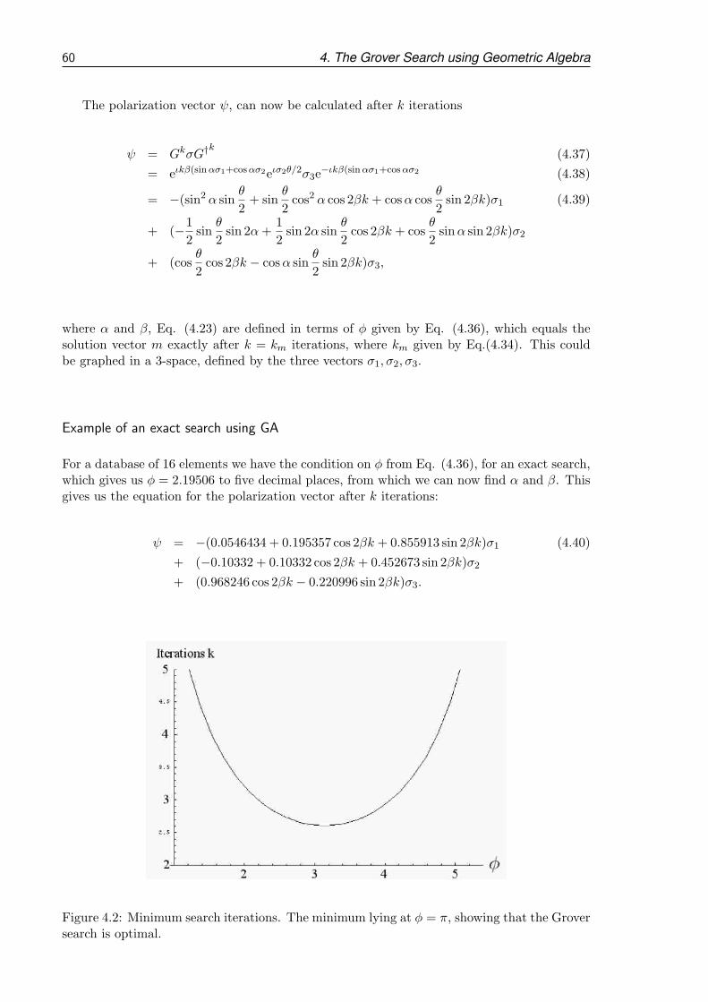
60 4. The Grover Search using Geometric Algebra
The polarization vector ψ, can now be calculated after k iterations
ψ = GkσG†k (4.37)
= eιkβ(sinασ1+cosασ2eισ2θ/2σ3e−ιkβ(sinασ1+cosασ2 (4.38)
= −(sin2 α sinθ
2+ sin
θ
2cos2 α cos 2βk + cosα cos
θ
2sin 2βk)σ1 (4.39)
+ (−1
2sin
θ
2sin 2α+
1
2sin 2α sin
θ
2cos 2βk + cos
θ
2sinα sin 2βk)σ2
+ (cosθ
2cos 2βk − cosα sin
θ
2sin 2βk)σ3,
where α and β, Eq. (4.23) are defined in terms of φ given by Eq. (4.36), which equals thesolution vector m exactly after k = km iterations, where km given by Eq.(4.34). This couldbe graphed in a 3-space, defined by the three vectors σ1, σ2, σ3.
Example of an exact search using GA
For a database of 16 elements we have the condition on φ from Eq. (4.36), for an exact search,which gives us φ = 2.19506 to five decimal places, from which we can now find α and β. Thisgives us the equation for the polarization vector after k iterations:
ψ = −(0.0546434 + 0.195357 cos 2βk + 0.855913 sin 2βk)σ1 (4.40)
+ (−0.10332 + 0.10332 cos 2βk + 0.452673 sin 2βk)σ2
+ (0.968246 cos 2βk − 0.220996 sin 2βk)σ3.
Figure 4.2: Minimum search iterations. The minimum lying at φ = π, showing that the Groversearch is optimal.

4.1 The Grover search operator in GA 61
Substituting in for k = 1, 2, 3 iterations, we find
ψ = (σ1, σ2, σ3) (4.41)
σ = (−0.25, 0, 0.9682)Gσ = (−0.8456, 0.315, 0.4309)G2σ = (−0.8456, 0.315,−0.4309)G3σ = (−0.25, 0,−0.9682),
thus producing the exact solution m after km = 3 iterations, as required.
4.1.2 General exact Grover search
Most generally we can write the Grover operator as
G = −UIγU−1Gm, (4.42)
whereIγ = I + (eiφ1 − 1)|γ〉〈γ|, (4.43)
where we normally choose γ = |0〉 = |0 . . . 0〉. For U = H, we have
G = −UIγU−1Gm = −(I + (eiφ1 − 1)H|γ〉〈γ|H = −(I + (eiφ1 − 1)|σ〉〈σ| = −GσGm. (4.44)
So, with this modified operator, we effectively use a modified vector to σ, namely the vectorγ = U |0〉. As this is a unit vector, we simply adapt Gσ to rotate about this new vector, thatis, we have
Gγ = e−ιγφ1/2 = e−ιφ12(− sin(θγ/2) cos(δ)σ1−sin(θγ/2) sin(δ)σ2+cos(θγ/2)σ3), (4.45)
where a and b describe a general unit vector in 3 space. Hence, for the general exact search,we have
G = −GγGm = −e−ιφ12(− sin(θγ/2) cos(δ)σ1−sin(θγ/2) sin(δ)σ2+cos(θγ/2)σ3)eιφ2/2(sin(θ/2)σ1+cos(θ/2)σ3).
(4.46)However, because we have two consecutive precession operations, we can replace this with asingle precession operation
G = eιβ(sin γ sinασ1+sin γ cosασ2+cos γσ3), (4.47)
for some real numbers α, β, γ, where once again we require the coefficient of σ3 to be zero.We also have a general starting state adjusted, because by replacing H with U , we have
changed the overlap on the starting state, so generally we have
|γ〉 = −e−iφ/2 cosθ04| ↑〉+ eiφ/2 sin
θ04| ↓〉.
In GA we can write it asγs = −e−ιφ0σ3/2eιθ0σ2/4 (4.48)
and as a polarization vector
γ = γsσ3γs (4.49)
= sinθ02cosφ0σ1 + sin
θ02sinφ0σ2 + cos
θ02σ3
= eιθ02(sinφ0σ1−cosφ0σ2)σ3,

62 4. The Grover Search using Geometric Algebra
so the full Grover search will give a polarization vector
ψ = Gkγsσ3γ†sG
†k (4.50)
= Gkeιθ02(sinφ0σ1−cosφ0σ2)σ3G
†k
= −σ3eισ2θ/2.
We can expand this expression using G defined above and equate this to the m vector to solvefor the phases φ1 and φ2. We would expect θ0 = θ, if no knowledge is given about the solution.
4.2 Summary
The Grover search algorithm is a central algorithm in the field of quantum computing, andhence it is important to represent it in the most efficient formalism possible. The two mainstrengths of geometric algebra are its method of handling rotations and its integral geometricrepresentation, and hence its perfect suitability in describing the Grover search. We find Clif-ford’s geometric algebra, provides a simplified representation for the Grover operator Eq. (4.12)and a clear geometric picture of the search process. Using the states of maximum and min-imum weight, we find that we can interpret the search process as the precession of a spin-12particle, thus providing a simple visual picture, as shown in Fig 4.1. This is not possible withthe standard formalism as it requires two complex axes, forming a four-dimensional space,and hence difficult to visualize. We also find that the exact Grover search Eq. (4.22) has anefficient algebraic solution, as shown in Eq. (4.36). This agrees with the exact search analysisundertaken in the previous chapter 3, however as anticipated, GA provides a clearer and moreefficient solution. We also wrote down the equation for a completely general Grover search inEq. (4.42), which can now be visualized in terms of the Bloch sphere, in which the problemis to rotate a given starting vector onto a target vector through selection of the appropriateprecession axis, as shown in Fig. 4.1 or Fig. 3.10. Improved intuition obtained via the use ofClifford’s geometric algebra, may possibly enhance the search for new quantum algorithms.

5
Quantum Game Theory
”Games combining chance and skill give the best representation of human life, particularly of
military affairs.” Gottfried Wilhelm von Leibniz.
We now extend our research into the arena of quantum game theory, which is closelyrelated to quantum computing in that they both involve the manipulation of qubits in orderto achieve a desired outcome. For example, one of the first quantum games studied [Mey99],involved two players applying operations on a single qubit, but which can be extended tomultiple qubit games.
Quantum game theory extends classical game theory [Ras07], [SOMI04b], [CT06], [VE00]an established branch of mathematics that describes and analyzes the strategic interactionamong a set of players, and which began fairly recently in 1999 with a seminal paper byDavid Meyer [Mey99], that described a penny-flip game involving a classical and a quantumplayer. By allowing the quantum player access to general unitary transformations performedon his qubit, whereas his opponent, the classical player, only had access to classical coin flips,Meyer showed that the quantum player achieved an overwhelming advantage, going from a50:50 chance of winning, to a game where he had a foolproof winning strategy. Following this,further motivation soon came in [EWL99], with the proposal of a quantum mechanical versionof the famous two player game of Prisoner dilemma which allowed new strategic solutions.Quantum games with decoherence was also investigated in [Joh01], [YSO+05].
In the following, as stated in the literature [Mey99], [EWL99], [FNA02], [FA05b], [Fli05],[Iqb05], we list some of the key reasons for the significance of game-theoretic studies in thequantum regime:
1. Game theory uses the concepts and methods of probability theory, in order to analyzegames. Playing quantum games provides an opportunity to generalize conventionalprobability into a quantum probability framework [Gud88].
2. Games of competition have an intimate connection with quantum communication con-cepts. For example, the quantum-mechanical protocols for eavesdropping [GH97], [Eke91],finance [PS02,PS08], optimal cloning [F.98], computer architectures [dSR08] and quan-tum teleportation [Pir05], can readily be formulated as games between players and havethe potential to shed new light on fundamental questions in quantum computing andquantum mechanics [NC02]. For example, Frieden [Fri89], [FS95], [FB00] showed thatphysical laws can be derived by considering the information content of a physical quan-tity, implying that the process of making a measurement represents a game againstnature. It turns out that the observer can never ‘win’, in the sense of obtaining com-plete information about a particular physical phenomenon.
3. It is possible [Mey99], [Mey02] to re-formulate certain quantum algorithms as gamesbetween classical and quantum players and hence it has been suggested that quantumgames may shed new light on the working of quantum algorithms, possibly helping tofind new ones.
4. Games can provide [Pie02] a useful set of tools in giving semantics to quantum logic andcan be brought to bear on questions concerning the interpretation and the nature of theconcept of uncertainty in the foundations of quantum theory.

64 5. Quantum Game Theory
5. Nanoscopic level interactions are dictated by quantum mechanics. Can Dawkins’ dictum[Daw76] of the ‘Selfish Gene’ be thought of in terms of games of survival with quantuminteractions?
Although recent years have seen a steady increase in the literature of quantum games[LJ02, PS03], several fundamental questions remain unanswered. For example, do quantumgames offer a genuine extension of the classical game theory or are they only transformedclassical games? Assuming the answer to this question is ‘yes’, then a reasonable domain,where quantum games have genuine potential to benefit game theory, is in the area of N -player games, where N can become infinite. It is precisely in this domain that only minimalinvestigations have been performed to date. It is because the standard mathematical formalismof quantum games uses density matrices, and those being complex matrices, the analysis of N -player games becomes nearly impossible. Also, with density matrices, constructing a geometricrepresentation of the problem at hand is often hard and sometimes becomes an impossible task.Hence, one of the key components of this section is the implementation of GA for the analysisof quantum games. Generally speaking, with the density matrix formalism, we use Dirac’sbra-ket formalism or density matrices and complex matrices for SU(2) rotations, whereaswith GA, we use quaternion style rotations of vectors in a real 3-space, which thus naturallyprovides a convenient geometric picture. GA has also been applied to quantum informationand computation [DL03] [HD02b], [DDL02]. As the area of quantum games is a part of thisfield, this provides a basis for a systematic investigation into quantum games using GA. Ithas also been noted [PS02] that research into quantum game theory should not be neglected,because current technological progress suggests that sooner or later someone will take fulladvantage of quantum theory and use quantum strategies to defeat us at some game, that is,an economic, diplomatic or perhaps military one.
A central concept in game theory, is the Nash equilibrium, which is the theoreticallyoptimal response by each player, assuming rational self interest, based on the games payoffstructure. The non-cooperative games we will consider assume that there is no communicationbetween the players, though each player has complete knowledge of the games parameters andthe games starting state. Different types of game are defined with a payoff matrix for eachplayer, based on the outcome of the game. Some common games investigated include thePrisoner dilemma, Stag hunt and Chicken games. For the two-player Prisoner dilemma (PD)game we have the payoff matrix for player A
GAij =
[3 05 1
]
=
[G00 G01
G10 G11
]
. (5.1)
For symmetric games, such as the well known PD game, we have for player B that GBij = GAji.Each player has two choices in the PD game, to cooperate or defect. If player A defectsand player B cooperates, the payoff for player A will be G10 = 5 as shown, where the firstsubscript indicates player A’s choice of defection and the second subscript, player B’s choiceof cooperation. In fact for the second column, where player B defects in both cases, player Ais still better off defecting, receiving G11 = 1 as opposed G01 = 0 if he cooperates. Hence, wecan see that player A will always receive a higher payoff by defecting, irrespective of players’B choice and hence rational self interest will create a NE of G11 = 1 payoff for both players bysymmetry. The game produces a dilemma because if they could somehow cooperate with eachother then they could both achieve a payoff of 3 units each. The Prisoner’s dilemma has wideapplicability in diverse areas of science such as biology, politics, economics and sociology. Forexample the PD game has applicability to climate change negotiations, in that each countrywill benefit from a stable climate and so they should cooperate to achieve this, however nocountry wants to act unilaterally because its extra manufacturing costs for example, will putit in a weaker position economically, hence all countries will tend not to cooperate and hencedo nothing (that is defect), as in the PD game.

65
A well known criticism [vEP02], [OSI07] of games incorporating quantum mechanics, ques-tions whether these quantum games should be considered completely new games rather thanextended versions of an existing classical game, because the players in quantum games aretypically given access to extended strategy sets (such as unitary transformations), relative towhat they are allowed to employ in the corresponding classical game. However the approachwe adopt to quantum games is based on an EPR type setting [ICA08, Iqb05], developed inChapter 6, which avoids this criticism because the players’ strategy sets in this formulationremain classical, being a choice of two measurement directions, and the classical game is re-covered when the quantum entanglement of the shared state goes to zero. Thus this categoryof quantum games can be genuinely considered to embed the corresponding classical gameand hence a genuine extension of the classical game.
As a first step in studying quantum games, we present quantum games from the perspectiveof a table of non-factorisable joint probabilities, published in [CIA10]. This provides a naturallink from classical probabilistic games to quantum games. From this perspective, quantumeffects are represented as non-factorisable joint probability distributions. We then look atquantum games from a true quantum mechanical perspective but using the formalism of GAin place of the more conventional bra-ket formalism. We introduce for the first time [CILVS09]the tools of GA to present an improved analysis of Meyer’s penny flip game [Mey99]. In thiswork, we found that GA indeed provided a geometric picture of the quantum mechanicalinteractions for this two-player game, which allowed a visualization of the solution strategythat emerges in this quantum game. We then extend this approach to two-player, three-player and finally N -player games, which can be used to model more complicated strategicinteractions. Multiqubit games are naturally modeled in GA as probabilistic outcomes overmultiple qubits and have a very efficient solution shown in Eq. (1.25).
66 5. Quantum Game Theory
5.1 Constructing quantum games from symmetric
non-factorisable joint probabilities
Quantum games constructed from a table of non-factorisable joint classical probabilities avoidsthe use of the conventional quantum mechanical formalism typically required in quantum gametheory. Classical games are described when the joint probabilities are factorisable but gameswith quantum mechanical features are produced when the joint probabilities become non-factorisable. Incorporating a symmetry constraint, we then give the Nash equilibrium andpayoff relations for a general quantum game which still embeds the classical game when thejoint probabilities become factorisable. Quantum versions of Prisoner dilemma, Stag Huntand the Chicken game are then investigated with this scheme. We show that this approachprovides a general framework for both classical and quantum games without recourse to theformalism of quantum mechanics, thus making the field more accessible to the non-physicist.A follow up paper linking this approach to a quantum mechanical approach as described inChapter 6, has been submitted for publication.
Published in Phys. Lett. A, 20010. [CIA10] (attached).Authors: J. M. Chappell(Adelaide University), A. Iqbal(Adelaide University) and D. Ab-
bott(Adelaide University).Statement of contributions: Dr. Iqbal had been working on non-factorisable joint proba-
bilities as a way to represent quantum games without using the normal quantum mechanicalformalism. J. Chappell suggested that a symmetry constraint on the table, might naturallyproduce classical and quantum games in this framework. J. Chappell worked through theconsequences of this idea, and along with the support of Dr. Iqbal and Prof. D. Abbottproduced a paper, accepted for publication in Phys. Lett. A.
Signed:
J. M. Chappell Dr A. Iqbal Prof. D. Abbott

5.2 The penny flip quantum game and geometric algebra 67
5.2 The penny flip quantum game and geometric algebra
We analyze Meyer’s quantum penny flip game using the language of geometric algebra(GA)and so determine all possible unitary transformations which enable the player Q to implementa winning strategy. We find that GA can provide a direct derivation of the winning trans-formation, which can be parameterized by the two angles θ and φ. Our results show thatGA facilitates a clear visual picture of the penny flip game, that is helpful in motivating anddeveloping further analysis of this quantum game. The result is significant, because for thefirst time the mathematical formalism of GA is applied to the field of quantum games andit appears to be superior to conventional approaches. Its specific benefits are the removal ofthe redundancy of the global phase and a simple visual representation of the problem. Thesuccess with a single qubit game naturally leads to an extension to two-player games with twoqubits.
Published in Journal of the Physical Society of Japan, Volume 78. [CILVS09] (attached).Authors: J. M. Chappell(Adelaide University), A. Iqbal(Adelaide University), M. A.
Lohe(Adelaide University) and Lorenz von Smekal(Adelaide University).Statement of contributions: Dr. A. Iqbal initially introduced J. Chappell to Meyer’s
quantum Penny Flip game. J. Chappell then proceeded to rework the original paper, usingGA. It soon became clear that GA provided a clear and concise derivation of a general solution.With Dr Azhar’s, Dr Lohe’s and Dr Lorenz von Smekal’s oversight, J. Chappell then prepareda suitable document for publication.
Signed:
J. M. Chappell Dr A. Iqbal Dr M.A.Lohe Dr Lorenz von Smekal

6
Two-player Quantum Games
The quantum game analyzed in the previous chapter, Meyer’s penny flip game (attached), de-scribed a two-player game in which players apply unitary transformations on a single commonqubit, which is then submitted for measurement to determine the outcome of the game. Wenow progress to two-player games, in which two qubits are employed, with a separate qubitallocated to each player and, significantly, by utilizing a pair of quantum particles, we nowhave available the quantum mechanical resource of entanglement. The previous schemes wereanalyzed using conventional techniques of Bra-ket notation and density matrices, however, wenow introduce an analysis based on Geometric Algebra(GA).
6.1 Introduction
Although its origins can be traced to earlier works [Bla80,Wie83,Mer90b,Mer90a], the ex-tension of game theory [Bin07,Ras07] to the quantum regime [Per93] was proposed by Meyer[Mey99] and Eisert et al [EWL99] and has since been investigated by others [Vai99, BH01,vEP02, Joh01, MW00, IT01, DLX+02b, DLX+02a, PS02, FA03, IT02, PS03, SOMI04a, FA05a,IW04,Men05,CT06, Iqb05,NT04,SOMI04b, IT07, OSI07, IC07,RNTK08,FH07,AV08,GZK08,ITC08, ICA08, LHJ09, IA09,CILVS09,CIA10, JMCL11a]. Game theory is a vast subject butmany interesting strategic interactions can still be found in simple-to-analyze two-player two-strategy non-cooperative games. The well known games of Prisoners’ Dilemma (PD) and StagHunt [Bin07,Ras07] are two such examples.
The general idea in the quantization scheme proposed by Eisert et al [EWL99] for suchgames involves a referee who forwards a two-qubit entangled state to the two players. Playersperform their strategic actions on the state that consist of local unitary transformations totheir respective qubits. The qubits are subsequently returned to the referee for measurementfrom which the players’ payoffs are determined. The setup ensures that players sharing aproduct initial state corresponds to the mixed-strategy version of the considered classical game.However, players sharing an entangled state can lead to new Nash equilibria (NE) [Bin07,Ras07] consisting of pairs of unitary transformations [Per93,EWL99]. At these quantum NEthe players can have higher payoffs relative to what they obtain at the NE in the mixed-strategy version of the classical game.
This approach to constructing quantum games was subsequently criticized [vEP02] asfollows. The players’ strategic actions in the quantum game are extended operations relativeto their actions in the original mixed-strategy version of the classical game, in which, eachplayer can perform a strategic action consisting of a probabilistic combination of their twopure strategies. The mentioned criticism [vEP02] argued that as the quantum players haveexpanded strategy sets and can do more than what the classical players can do, it is plausibleto represent the quantum game as an extended classical game that also involves new purestrategies. The entries in the extended game matrix can then be suitably chosen so to berepresentative of the players’ payoffs at the obtained quantum NE. This line of reasoning canbe extended further in stating that quantum games are in fact ‘disguised’ classical games andto quantize a game is equivalent to replacing the original game by an extended classical game.
As a way to counter the criticism in [vEP02], two-party Einstein-Podolsky-Rosen (EPR)type experiments [EPR35,Boh51,B+64,Bel87,Bel66,ADR82,CS78,Cer00] are recognized tohave genuinely quantum features. One observes that the setting of such experiments can

70 6. Two-player Quantum Games
be fruitfully adapted [IW04, Iqb05, IC07, ICA08, IA09] for playing a quantum version of atwo-player two-strategy game, which allows us to avoid the criticism from another perspec-tive. In particular, with the EPR type setting the players’ strategies can be defined entirelyclassically—consisting of a probabilistic combination of a player’s choice between two mea-surement directions. That is, with this setting, the players’ strategy sets remain identical toones they have in a standard arrangement for playing a mixed-strategy version of a classicaltwo-player two-strategy game. As the players’ strategy sets in the quantum game are notextended relative to the classical game, for this route to constructing quantum games, thementioned criticism [vEP02] does not apply.
Figure 6.1: The EPR setup.
The usefulness of applying the formalism of geometric algebra (GA) [Hes99,HS84,DL03,DSD07] in the investigation of quantum games has recently been shown [CILVS09] for the wellknown quantum penny flip game [Mey99]. One may ask about the need of using the formalismof GA when, for instance, the GA based analysis of two-player quantum games developed inthe following can also be reproduced with the standard analysis with Pauli matrices. We canargue that the Pauli matrices are not always the preferred representation. Especially, as itis quite often overlooked that the algebra of Pauli matrices is the matrix representation forthe Clifford’s geometric algebra R3, which is no more and no less than a system of directednumbers representing the geometrical properties of Euclidean 3-space. As a GA based analysisallows using operations in 3-space with real coordinates, it thus permits a visualization thatis simply not available in the standard approach using matrices over the field of complexnumbers. Pauli matrices are isomorphic to the quaternions, and hence represent rotations ofparticle states. This fact paves the way to describe general unitary transformations on qubits,in a simplified algebraic form, as rotors that bring noticeable simplifications and geometricalclarifications. We apply constraints on the parameters of EPR type arrangements that ensurea faithful embedding of the mixed-strategy version of the original classical game within thecorresponding quantum game. In particular, we show how using GA we can determine newNE in quantum games of Stag Hunt and Prisoners’ Dilemma played in the EPR type setting.
6.2 EPR setting for playing a quantum game
We have the following payoff matrices
A = AliceS1S2
Bob
S′1 S′
2(G00 G01
G10 G11
)
, B = AliceS1S2
Bob
S′1 S′
2(H00 H01
H10 H11
)
, (6.1)

6.3 Geometric algebra 71
giving Alice’s and Bob’s payoffs, respectively. Here Alice’s pure strategies are S1 and S2 andBob’s pure strategies are S′
1 and S′2. In a run, Alice chooses her strategy to be either S1 or
S2 and likewise, in the same run, Bob chooses his strategy to be either S′1 or S′
2. We considergames with symmetrical payoffs for which B = AT , where T indicates transpose. This requiresH00 = G00, H01 = G10, H10 = G01, and H11 = G11.
The EPR setting assumes that players Alice and Bob are spatially-separated participants,who are located at the two arms of the EPR system. In a run, each player receives one half ofa two-particle system emitted by the same source. We associate Alice’s strategies S1, S2 to thedirections κ11, κ
12 respectively and similarly, associate Bob’s strategies S′
1, S′2 to the directions
κ21, κ22, respectively. On receiving a pair of particles, players Alice and Bob together choose a
pair of directions from the four possible cases (κ11, κ21), (κ
11, κ
22), (κ
12, κ
21), (κ
12, κ
22) and a quantum
measurement is performed along the chosen pair. The outcome of the measurement at eitherarm is +1 or −1. Over a large number of runs, a record is maintained of the players’ choicesof directions, representing their strategies, and one of the four possible outcomes (+1,+1),(+1,−1), (−1,+1), (−1,−1) emerging out of the measurement. Within each of the brackets,the first entry is reserved for the outcome at Alice’s side and the second entry for the outcomeat Bob’s side. Players’ payoff relations are expressed in terms of the outcomes of measurementsthat are recorded for a large number of runs, as the players sequentially receive, two-particlesystems emitted from the source. These payoffs depend on the strategic choices that eachplayer adapts for his/her two directions over many runs, and on the dichotomic outcomes ofthe measurements performed along those directions.
6.3 Geometric algebra
Geometric algebra (GA) [Hes99,HS84,DL03,DSD07] is an associative non-commutative alge-bra, that can provide an equivalent description to the conventional Dirac bra-ket and matrixformalisms of quantum mechanics, consisting of solely of algebraic elements over a strictlyreal field. Recently, Christian [Chr07] has used the formalism of GA in thought provokinginvestigations of some of the foundational questions in quantum mechanics. In the area ofquantum games, GA has been used by Chappell et al [CILVS09] to determine all possible uni-tary transformations that implement a winning strategy in Meyer’s PQ penny flip quantumgame [Mey99], and also in analyzing three-player quantum games [JMCL11a].
Using the one-to-one mapping from quantum states to GA defined in Eq. (1.24) it canthen be shown using the Schmidt decomposition of a general two qubit state, that a generaltwo-particle state can be represented (see Appendix) in GA as
ψ = AB(cosγ
2+ sin
γ
2ισ12ισ
22), (6.2)
where γ ∈ [0, π2 ] is a measure of the entanglement and where A,B are single particle rotorsapplied to the first and second qubit, respectively.
General unitary operations in GA can be represented as
R(θ1, θ2, θ3) = e−θ3ισ3/2e−θ1ισ2/2e−θ2ισ3/2. (6.3)
This rotation, in Euler angle form, can completely explore the available space of a single qubit,and is equivalent to a general unitary transformation acting on a spinor. We have the rotorsfor each qubit defined as
A = R(α1, α2, α3) = e−α3ισ3/2e−α1ισ2/2e−α2ισ3/2 (6.4)
B = R(β1, β2, β3) = e−β3ισ3/2e−β1ισ2/2e−β2ισ3/2.
72 6. Two-player Quantum Games
We see that with the three degrees of freedom provided in each rotor and with the entanglementangle γ, we have defined a two particle quantum state with 7 degrees of freedom, as requiredfor a two-particle quantum state ignoring the global phase. For example, for A = B = 1 andγ = −π
2 , we find the Bell state, or with A = 1 and B = R(π, 0, 0) and γ = π2 , we produce the
singlet state.To simulate the process of measurement, we form a separable state φ = RS, where R and
S are single particle rotors, which allow general measurement directions to be specified. Theoverlap probability between two states in the N -particle case is given by Eq.(1.25), which forthe two particle case becomes
P (ψ, φ) =⟨ψEψ†φEφ†
⟩−⟨ψJψ†φJφ†
⟩, (6.5)
where E and J are defined by Eq.(1.26) and Eq.(1.28).
6.3.1 Calculating observables
Employing Eq. (1.25), we firstly calculate
ψEψ† =1
2AB
(
cosγ
2+ sin
γ
2ισ12ισ
22
) (1− ισ13ισ23
) (
cosγ
2+ sin
γ
2ισ12ισ
22
)
B†A†
=1
2AB
(1− ισ13ισ23 + sin γ
(ισ12ισ
22 − ισ11ισ21
))B†A†
=1
2
(
1− ιAσ13A†ιBσ23B† + sin γ
(
ιAσ12A†ιBσ22B
† − ιAσ11A†ιBσ21B†))
(6.6)
and
ψJψ† =1
2AB
(
cosγ
2+ sin
γ
2ισ12ισ
22
) (ισ13 + ισ23
) (
cosγ
2+ sin
γ
2ισ12ισ
22
)
B†A†
=1
2AB
(
cos2γ
2− sin2
γ
2
) (ισ13 + ισ23
)B†A†
=1
2cos γ
(
ιAσ13A† + ιBσ23B
†)
. (6.7)
To describe the players measurement directions, we have R = e−ικ1σ1
2 and S = e−ικ2σ2
2 . Forthe quantum game in the EPR setting, κ1 can be either of Alice’s two directions i.e. κ11 or κ12.Similarly, in the expression for S the κ2 can be either of Bob’s two directions i.e. κ21 or κ22.Hence we obtain
φJφ† = RSJS†R†
=1
2
(
ιRσ13R† + ιSσ23S
†)
=1
2
(
ισ13eικ1σ1
2 + ισ23eικ2σ2
2
)
, (6.8)
and
φEφ† = RSES†R†
=1
2
(
1− ιRσ13R†ιSσ23S†)
=1
2
(
1− ισ13eικ1σ1
2 ισ23eικ2σ2
2
)
. (6.9)
Now from Eq. (1.25), we calculate
−⟨
ψJψ†φJφ†⟩
0= −1
4
⟨
cos γ(
ιAσ13A† + ιBσ23B
†)(
ισ13eικ1σ1
2 + ισ23eικ2σ2
2
)⟩
0
=1
4cos γ
[(−)mX(κ1) + (−)nY (κ2)
], (6.10)

6.3 Geometric algebra 73
where m,n ∈ 0, 1 refers to measuring a |0〉 or a |1〉 state, respectively, and using the resultsin Appendix, we have
X(κ1) = cosα1 cosκ1 + cosα3 sinα1 sinκ
1, (6.11)
Y (κ2) = cosβ1 cosκ2 + cosβ3 sinβ1 sinκ
2. (6.12)
Also, from Eq. (1.25) we obtain
⟨
ψEψ†φEφ†⟩
0(6.13)
=⟨
(1− ιAσ13A†ιBσ23B† + sin γ(ιAσ12A
†ιBσ22B† − ιAσ11A†ιBσ21B
†))
× (1− ισ13ισ23eικσ12eιτσ
22 )⟩
0
=1
4
[1 + (−)m+nXY − (−)m+n sin γU(k1)V (k2)− F (k1)G(k2)
], (6.14)
where
F (κ1) = cosα2(cosκ1 sinα1 − cosα3 sinκ
1 cosα1) + sinκ1 sinα2 sinα3, (6.15)
G(κ2) = cosβ2(cosκ2 sinβ1 − cosβ3 sinκ
2 cosβ1) + sinκ2 sinβ2 sinβ3 (6.16)
and
U(κ1) = − sinα2(cosκ1 sinα1 − cosα3 sinκ
1 cosα1) + sinκ1 cosα2 sinα3, (6.17)
V (κ2) = − sinβ2(cosκ2 sinβ1 − cosβ3 sinκ
2 cosβ1) + sinκ2 cosβ2 sinβ3. (6.18)
To simplify the equations, we define
Z(κ1, κ2) = F (k1)G(k2)− U(k1)V (k2) (6.19)
= cosφ[cosκ1 cosκ2 sinβ1 sinα1 − sinκ1 cosκ2 sinβ1 cosα1 cosα3
+ sinκ1 sinκ2(cosα1 cosα3 cosβ1 cosβ3 − sinα3 sinβ3)
− cosκ1 sinκ2 sinα1 cosβ1 cosβ3]
+ sinφ[sinκ1 cosκ2 sinα3 sinβ1 + cosκ1 sinκ2 sinα1 sinβ3
+ sinκ1 sinκ2(cosβ1 cosβ3 sinα3 + cosα1 cosα3 sinβ3)]. (6.20)
Now combining Eq. (6.10) and Eq. (6.14) we have the probability to observe a particular state
Pmn =1
4
[1 + cos γ(−)mXi + (−)nYj+ (−)m+n(XiYj + sin γZij)
]. (6.21)
To simplify notation we have written Zij = Z(κ1i , κ2j ) , Xi = X(κ1i ) and Yj = Y (κ2j ), where
i, j ∈ 1, 2 represent the two possible measurement directions available to each player. Wenotice that we were able to make the substitution φ = α2 + β2 in Eq. (6.20), which as shownin Appendix, is as expected from the known redundancy in the rotors. If we put γ = 0, thatis, for no entanglement, we have the probability
Pmn =1
4
(1 + (−)mXi + (−)nYj + (−)m+nXiYj
)
=(1 + (−)mXi)
1
2
(1 + (−)nYj)22
, (6.22)
which shows a product state incorporating general measurement directions for each qubit.

74 6. Two-player Quantum Games
Writing out the probabilities for the four measurement outcomes we find
P00(κ1i , κ
2j ) =
1
4[1 + cos γ(Xi + Yj) + (XiYj + sin γZij)] , (6.23)
P01(κ1i , κ
2j ) =
1
4[1 + cos γ(Xi − Yj)− (XiYj + sin γZij)] , (6.24)
P10(κ1i , κ
2j ) =
1
4[1 + cos γ(−Xi + Yj)− (XiYj + sin γZij)] , (6.25)
P11(κ1i , κ
2j ) =
1
4[1 + cos γ(−Xi − Yj) + (XiYj + sin γZij)] . (6.26)
6.3.2 Finding the payoff relations
We allow each player the classical probabilistic choice between their two chosen measurementdirections for their Stern-Gerlach detectors. The two players, Alice and Bob choose their firstmeasurement direction with probability x and y respectively, where x, y ∈ [0, 1]. Now, wehave the mathematical expectation of Alice’s payoff, where she chooses the direction κ11 withprobability x and the measurement direction κ12 with probability 1− x, as
ΠA(x, y) = xy[P00G00 + P01G01 + P10G10 + P11G11]
+ x(1− y)[P00G00 + P01G01 + P10G10 + P11G11]
+ y(1− x)[P00G00 + P01G01 + P10G10 + P11G11]
+ (1− x)(1− y)[P00G00 + P01G01 + P10G10 + P11G11], (6.27)
where we have used the payoff matrix, defined for Alice, in Eq. (6.1) and the subscript A refersto Alice. We also define
∆1 = G10 −G00, ∆2 = G11 −G01, ∆3 = ∆2 −∆1, (6.28)
so that by using Eqs. (6.23-6.26) the payoff for Alice (6.27) is expressed as
ΠA(x, y)
=1
4
[
G00 +G10 +G01 +G11
+∆3x((X1 −X2)Y2 + (Z12 − Z22) sin γ) + y((Y1 − Y2)X2 + (Z21 − Z22) sin γ)
+ xy(X1 −X2)(Y1 − Y2) + sin γ(Z11 + Z22 − Z12 − Z21)+X2Y2 + Z22 sin γ
− cos γ(∆1 +∆2)((X1 −X2)x+X2)−∆4((Y1 − Y2)y + Y2)]
, (6.29)
where ∆4 = G00 − G01 + G10 − G11. Bob’s payoff, when Alice plays x and Bob plays y cannow be obtained by interchanging x and y in the right hand side of Eq. (6.29).
6.3.3 Solving the general two-player game
We now find the optimal solutions by calculating the Nash equilibrium (NE), that is, theexpected response assuming rational self interest. To find the NE we simply require
ΠA(x∗, y∗) ≥ ΠA(x, y
∗), ΠB(x∗, y∗) ≥ ΠB(x
∗, y), (6.30)
which is stating that any unilateral movement of a player away from the NE of (x∗, y∗), willresult in a lower payoff for that player. We find
ΠA(x∗, y∗)−ΠA(x, y
∗)
=1
4(x∗ − x)
[
∆3
y∗((X1 −X2)(Y1 − Y2) + sin γ(Z11 + Z22 − Z12 − Z21))
+ (X1 −X2)Y2 + (Z12 − Z22) sin γ− cos γ(∆1 +∆2)(X1 −X2)
]
(6.31)
6.3 Geometric algebra 75
and for the second player Bob we have similarly
ΠB(x∗, y∗)−ΠB(x
∗, y)
=1
4(y∗ − y)
[
∆3
x∗((X1 −X2)(Y1 − Y2) + sin γ(Z11 + Z22 − Z12 − Z21))
+ (Y1 − Y2)X2 + (Z21 − Z22) sin γ− cos γ(∆1 +∆2)(Y1 − Y2)
]
. (6.32)
6.3.4 Embedding the classical game
To embed the classical game, we require at zero entanglement, not only the same pair ofstrategies being a NE but also to have the bilinear structure of the classical payoff relations.At a NE of (x∗, y∗) = (0, 0), with zero entanglement, we find the payoff from Eq. (6.29) to be
ΠA(0, 0) =1
4
[G00(1 +X2)(1 + Y2) +G10(1−X2)(1 + Y2)
+G01(1 +X2)(1− Y2) +G11(1−X2)(1− Y2)]. (6.33)
This result illustrates how we could select any one of the payoff entries we desire with theappropriate selection of X2 and Y2, however in order to achieve the classical payoff of G11 forthis NE, we can see that we require X2 = −1 and Y2 = −1. If we have a game which also hasa classical NE of (x∗, y∗) = (1, 1) then from Eq. (6.29) at zero entanglement we find the payoff
ΠA(1, 1) =1
4
[G00(1 +X1)(1 + Y1) +G10(1−X1)(1 + Y1)
+G01(1 +X1)(1− Y1) +G11(1−X1)(1− Y1)]. (6.34)
So, we can see, that we can select the required classical payoff, of G00, by the selection ofX1 = 1 and Y1 = 1.
Referring to Eq. (6.12), we then have the conditions
X(κ1) = cosα1 cosκ1 + cosα3 sinα1 sinκ
1 = ±1, (6.35)
Y (κ2) = cosβ1 cosκ2 + cosβ3 sinβ1 sinκ
2 = ±1. (6.36)
Looking at the equation for Alice, we have two classes of solution: If α3 6= 0, then for theequations satisfying X2 = Y2 = −1, we have for Alice in the first equation α1 = 0, κ12 = πor α1 = π, κ12 = 0 and for the equations satisfying X1 = Y1 = +1, we have α1 = κ11 = 0 orα1 = κ11 = π, which can be combined to give either α1 = 0, κ11 = 0 and κ12 = π or α1 = π,κ11 = π and κ12 = 0. For the second class with α3 = 0, we have the solution α1 − κ12 = π andfor X1 = Y1 = +1 we have α1 − κ11 = 0.
So, in summary, for both cases we have that the two measurement directions are π outof phase with each other, and for the first case (α3 6= 0) we can freely vary α2 and α3, andfor the second case (α3 = 0), we can freely vary α1 and α2 to change the initial quantumquantum state without affecting the game NE or the payoffs. The same arguments hold forthe equations for Y . Combining these results and substituting into Eq. (6.20), we see byinspection for the two cases that
F (κ1) = G(κ2) = U(κ1) = V (κ2) = 0, (6.37)
and hence, we find that
Z22 = Z21 = Z12 = Z11 = 0. (6.38)
This then reduces the equation governing the NE in Eq. (6.31) to
ΠA(x∗, y∗)−ΠA(x, y
∗) =1
2(x∗ − x)
[∆32y∗ − 1 − cos γ(∆1 +∆2)
]≥ 0, (6.39)

76 6. Two-player Quantum Games
which now has the new quantum behavior governed solely by the entanglement angle γ. Wehave the associated payoffs
ΠA(x, y) =1
2
[G00 +G11 − cos γ(G00 −G11) + 2xy∆3
− x∆3 + cos γ(∆1 +∆2) − y∆3 − cos γ(G00 −G01 +G10 −G11)]. (6.40)
Setting γ = 0 in Eq. (8.22) we find
ΠA(x, y) = G11 + x(G01 −G11) + y(G10 −G11) + xy(G00 −G01 −G10 +G11), (6.41)
which has the classical bilinear payoff structure in terms of x and y. Hence we have faithfullyembedded the classical game inside a quantum version of the game, when the entanglementgoes to zero.
We also have the probabilities for each state |m〉|n〉, after measurement from Eq. (6.21),for this form of the quantum game as
(Pmn)ij =1
4
[1 + cos γ((−)m+i+1 + (−)n+j+1) + (−)m+n+i+j
], (6.42)
for the two measurement directions i and j.
6.4 Examples
Here we explore the above results for the games of Prisoners’ Dilemma and Stag Hunt. Thequantum versions of these games are discussed in Refs. [EWL99,BH01,FA03,FA05a, IA09].
6.4.1 Prisoners’ Dilemma
The game of Prisoners’ Dilemma (PD) [Ras07] is widely known to economists, social andpolitical scientists and is one of the earliest games to be investigated in the quantum regime[EWL99]. PD describes the following situation: two suspects are investigated for a crime thatauthorities believe they have committed together. Each suspect is placed in a separate celland may choose between not confessing or confessing to have committed the crime. Referringto the matrices (6.1) we take S1 ∼ S′
1 and S2 ∼ S′2 and identify S1 and S2 to represent
the strategies of ‘not confessing’ and ‘confessing’, respectively. If neither suspect confesses,i.e. (S1, S1), they go free, which is represented by G00 units of payoff for each suspect. Thesituation (S1, S2) or (S2, S1) represents in which one prisoner confesses while the other doesnot. In this case, the prisoner who confesses gets G10 units of payoff, which represents freedomas well as financial reward as G10 > G00, while the prisoner who did not confess gets G01,represented by his ending up in the prison. When both prisoners confess, i.e. (S2, S2), theyboth are given a reduced term represented by G11 units of payoff, where G11 > G01, but it isnot so good as going free i.e. G00 > G11.
With reference to Eq. (6.28), we thus have ∆1, ∆2 > 0. However, depending on therelative sizes of ∆1, ∆2, the quantity ∆3 = ∆2−∆1 can be positive or negative. At maximumentanglement (cos γ = 0), we note from Eq. (6.39), that there are two cases depending on ∆3.If ∆3 > 0, we notice that both the NE of (x∗, y∗) = (0, 0) and (x∗, y∗) = (1, 1) are present,and from Eq. (8.22) we have the payoff in both cases
ΠA(0, 0) = ΠB(0, 0) =1
2(G00 +G11) = ΠA(1, 1) = ΠB(1, 1), (6.43)
which is a significant improvement over the classical payoff of G11. For ∆3 < 0, we have thetwo NE of (x∗, y∗) = (0, 1) and (x∗, y∗) = (1, 0), and from Eq. (8.22) we have the payoff
ΠA(0, 1) = ΠB(0, 1) =1
2(G01 +G10) = ΠA(1, 0) = ΠB(1, 0). (6.44)

6.4 Examples 77
If we reduce the entanglement of the qubits provided for the game, increasing cos γ towards one,then from Eq. (6.39), we find a phase phase transition to the classical NE of (x∗, y∗) = (0, 0),at ∆3 − cos γ(∆1 +∆2) = 0 or
cos γ =∆3
∆1 +∆2=
∆2 −∆1
∆2 +∆1. (6.45)
Because we know that ∆1, ∆2 > 0, for the PD game, then a phase transition to the classicalNE is guaranteed to occur, in the range [0, 1].
Consider a particular example of PD by taking G00 = 3 = H00, G01 = 0 = H10, G10 = 4 =H01, and G11 = 2 = H11 in matrices (6.1). From (6.28) we find ∆1 = 1, ∆2 = 2 and ∆3 = 1and we obtain γ ≤ cos−1(1/3) for a transition to the classical NE. Thus, for this PD game, togenerate a non-classical NE the entanglement parameter γ should be greater than cos−1(1/3).
6.4.2 Stag Hunt
The game of Stag Hunt (SH) [Ras07] is encountered in the problems of social cooperation. Forexample, if two hunters are hunting for food, in a situation where they have two choices, eitherto hunt together and kill a stag, which provides a large meal, or become distracted and huntrabbits separately instead, which while tasty, make a substantially smaller meal. Hunting astag of course is quite challenging and the hunters need to cooperate with each other in orderto be successful. The game of SH has three classical NE, two of which are pure and one ismixed. The two pure NE correspond to the situation where both hunters hunt the stag as ateam or where each hunts rabbits by himself.
The SH game can be defined by the conditions ∆3 > ∆2 > 0 and ∆1 + ∆2 > 0 and∆3 > ∆1+∆2. In the classical (mixed-strategy) version of this game three NE (two pure andone mixed) appear consisting of (x∗, y∗) = (0, 0), (x∗, y∗) = (1, 1) and (x∗, y∗) = (∆2
∆3, ∆2∆3
).From Eq. (6.39) and the defining conditions of SH game we notice that both the strategy pairs(0, 0) and (1, 1) also remain NE in the quantum game for an arbitrary γ. Eq. (8.22) give theplayers’ payoffs at these NE as follows:
ΠA(0, 0) =1
2[G00 +G11 − cos γ(G00 −G11)] = ΠB(0, 0), (6.46)
ΠA(1, 1) =1
2[G00 +G11 + cos γ(G00 −G11)] = ΠB(1, 1), (6.47)
which assume the values G11 and G00 at γ = 0, respectively. When γ = π2 we have ΠA(0, 0) =
ΠA(1, 1) =12(G00+G11) = ΠB(1, 1) = ΠB(0, 0). For the mixed NE for the quantum SH game
we require from Eq. (6.39), ∆32y∗ − 1 − cos γ(∆1 +∆2) = 0 or
x∗ =cos γ(∆1 +∆2) + ∆2 −∆1
2∆3= y∗, (6.48)
which returns the classical mixed NE of (∆2∆3, ∆2∆3
) at zero entanglement. Depending on the
amount of entanglement, the pair (x∗, y∗), however, will shift themselves between ∆2∆3
and∆2−∆12∆3
. Players’ payoffs at this shifted NE can be obtained from Eq. (8.22). Consider aparticular example of SH by taking G00 = 10 = H00, G01 = 0 = H10, G10 = 8 = H01, andG11 = 7 = H11 in matrices (6.1). From (6.28) we find ∆1 = −2, ∆2 = 7 and ∆3 = 9. Atγ = π
2 we have ΠA(0, 0) = ΠA(1, 1) =172 = ΠB(1, 1) = ΠB(0, 0). That is, the players’ payoffs
at the NE strategy pair (0, 0) are increased from 7 to 172 while at the NE strategy pair (1, 1)
these are decreased from 10 to 172 . The mixed NE in the classical game is at x∗ = 7
9 = y∗
whereas it shifts to 12 at γ = π
2 .
78 6. Two-player Quantum Games
6.5 Discussion
The EPR type setting for playing a quantum version of a two-player two-strategy game isexplored using the formalism of Clifford geometric algebra (GA), used for the representationof the quantum states, and the calculation of observables. We find that analyzing quantumgames using GA comes with some clear benefits, for instance, improved perception of thequantum mechanical situation involved and particularly an improved geometrical visualizationof quantum operations. To obtain equivalent results using the familiar algebra with Paulimatrices would be possible but obscures intuition. We also find that an improved geometricalvisualization becomes helpful in significantly simplifying quantum calculations.
We find that by using an EPR type setting we produce a faithful embedding of symmetricmixed-strategy versions of classical two-player two-strategy games into its quantum version,and that GA provides a simplified formalism over the field of reals for describing quantumstates and measurements.
For a general two-player two-strategy game, we find the governing equation for a strategypair forming a NE and the associated payoff relations. We find that at zero entanglement thequantum game returns the same pair(s) of NE as the classical mixed-strategy game, while thepayoff relations in the quantum game reduce themselves to their bilinear form correspondingto a mixed-strategy classical game. We find that, within our GA based analysis, even thoughthe requirement to properly embed a classical game puts constraints on the possible quantumstates allowing this, we still have a degree of freedom, available with the entanglement angleγ, with which we can generate new NE. As a specific example the PD was found to have aNE of (x∗, y∗) = (1, 1) at high entanglement.
Analysis of quantum PD game in this paper can be compared with the results developed forthis game in Ref. [IC07] also using an EPR type setting, directly from a set of non-factorizablejoint probabilities. Although Ref. [IC07] and the present paper both use an EPR type setting,they use non-factorizability and entanglement for obtaining a quantum game, respectively.Our recent work [CIA10] has observed that Ref. [IC07] does not take into consideration asymmetry constraint on joint probabilities that is relevant both when joint probabilities arefactorizable or non-factorizable. When this symmetry constraint is taken into consideration,an analysis of quantum PD game played using an EPR setting does generate a non-classicalNE in agreement with the results in this paper.
Many other classical games could now be investigated in this setting, however, we proceedinstead to demonstrate the use of GA in solving three-player and N -player games using anEPR setting.

7
Three-player Quantum Games in an EPR
setting
In the paper attached, we extend the Einstein-Podolsky-Rosen (EPR) framework for two-player quantum games, to three-player quantum games. As already noted, by using an EPRsetting, the players’ strategy sets remain identical to those available to players in the mixed-strategy version of the classical game, obtained as a proper subset of the corresponding quan-tum game, thus avoiding a common criticism of quantum games, that they are not genuineextensions of existing classical games. Using general symmetrical three-qubit pure states inthis framework, we analyze the three-player quantum game of Prisoners’ Dilemma.
The usefulness of achieving this is firstly to establish a sound framework for quantumgames for three players which authentically extend classical games, but also in establishing anapproach which is immediately extendable to the N -player quantum game.
Published in Public Library of Science, Volume 6(7). [JMCL11a] (attached).Authors: J. M. Chappell(Adelaide University), A. Iqbal(Adelaide University) and D. Ab-
bott(Adelaide University)Statement of contributions: J. Chappell extended the mathematics developed in the previ-
ous chapter based on two qubits to three qubits. Dr A. Iqbal and Prof D. Abbott consulted onthe extra difficulties posed by games played with the three qubit GHZ and W states analyzed.J. Chappell and A. Iqbal then prepared a paper for publication, with further checking by D.Abbott and M.A. Lohe.
Signed:
J. M. Chappell Dr A. Iqbal Prof. D.Abbott Dr M.A. Lohe

8
N-player Quantum Games
We now generalize our analysis of two-player and three-player quantum games to multi-playerquantum games which are also analyzed in the context of an Einstein-Podolsky-Rosen (EPR)experiment. As previously noted, in this setting, the players’ strategy sets remain identicalto the ones in the mixed-strategy version of the classical game, and so we obtain a properembedding of the classical game. Expressions are found for the probability distribution for Nqubit states subject to general measurement directions, from which expressions for the mixedNash Equilibrium and the payoffs are found, producing a general quantum game environmentfor N ≥ 2 players. In order to avoid the cumbersome use of large N × N matrices definingthe payoffs, we define the player payoffs with linear functions, and as a specific example thePrisoner dilemma is solved for all N , finding a new property for the Prisoner dilemma, thatfor an even number of players the payoffs at the Nash equilibrium are equal, whereas for anodd number of players the cooperating players receive a higher payoff.
8.1 Introduction
Initially, studies in the arena of quantum games focused on two-player, two-strategy non-cooperative games but was extended to multi-player quantum games by Benjamin and Hayden[BH01]. Such games can be used to describe multi-party situations, such as in the analysisof secure quantum communication [NC02]. As multi-player quantum games are usually foundsignificantly harder to analyze, as we are required to define an N × N payoff matrix, andcalculate measurement outcomes over N -qubit states, GA is identified as the most suitableformalism in order to allow ease of analysis. Also, in the case where N → ∞, clearly matrixmethods will become unworkable and so an algebraic approach, such as GA, becomes essential.
8.2 EPR setting for playing multi-player quantum games
For a multi-player quantum game in a EPR setting [IW04, IC07, ICA08] we have players P i
who are spatially-separated participants, located at the N arms of an EPR system [Per93], asshown in Fig. 8.1. In one run of the experiment, each player chooses one out of two possiblemeasurement directions. These two directions in space, along which spin or polarizationmeasurements can be made, are the players’ strategies.
As Fig. 8.1 shows, we represent the ith players two measurement directions as κi1, κi2, with
the measurement outcome being +1 or −1.Over a large number of runs the players are allocated a qubit from an N -particle system
emitted from a source upon which measurements are performed and a record is maintainedof the players’ payoffs. These payoffs depend on the N -tuples of the various players’ strategicchoices made over a large number of runs and on the dichotomic outcomes (measuring spin-upor spin-down) from the measurements performed along those directions.
8.2.1 Symmetrical N qubit states
For N -player quantum games an entangled state of N qubits is prepared by the supervisor,which for fair games should be symmetric with regard to the interchange of the N players,

82 8. N -player Quantum Games
Figure 8.1: The EPR setup for an N -player quantum game. In this setting, each player isgiven a choice of two measurement directions for their allocated qubit, from a shared N -qubitquantum state.
and we assume that all information about the state once prepared is known by the players.Two types of entangled starting states can readily be identified which are symmetrical withrespect to the N players. The GHZ-type state
|GHZ〉N = cosγ
2|00 . . . 0〉+ sin
γ
2|11 . . . 1〉, (8.1)
where we include an entanglement angle γ ∈ [−π2 ,
π2 ] and the W -type state
|W〉N =1√N
(|1000 . . . 00〉+ |0100 . . . 00〉+ |0010 . . . 00〉+ · · ·+ |0000 . . . 01〉) . (8.2)
To represent these in geometric algebra, we start with the mapping for a single qubit fromEq. (1.24), so that for the GHZ-type state we have
ψGHZN= cos
γ
2+ sin
γ
2ιe12ιe
22 . . . ιe
N2 , (8.3)
where the superscript indicates which particle space each qubit belongs to, and the negativecoefficient on the second term for an odd number of particles can be absorbed into sin γ. Alsofor the W-type state we have in GA
ψWN= − 1√
N
(ιe12 + ιe22 + · · ·+ ιeN2
). (8.4)
8.2.2 Unitary operations and observables in GA
We define U i = R(θi1, θi2, θ
i3) for a general unitary transformation acting locally on each qubit
i, where R is defined in Eq. (6.3), which the supervisor applies to the individual qubits, whichgives the starting state
(U1 ⊗ U2 ⊗ · · · ⊗ UN
)|ψ〉, (8.5)

8.2 EPR setting for playing multi-player quantum games 83
upon which the players now decide upon their measurement directions.
The overlap probability between two states ψ and φ, in the N -particle case is given inEq.(1.25). Initially we assume that N is odd, in order to simplify our derivation, but ourresults are then easily generalized for all N .
The supervisor now submits each qubit for measurement, through N Stern-Gerlach typedetectors, with each detector being set at one of the two angles chosen by each player. Asmentioned, the players choices, are a classical choice between two possible measurement di-rections, and hence the players strategy sets remain the same as in the classical game, withthe quantum outcomes arising solely from the shared quantum state.
In order to calculate the measurement outcomes, we define a separable state φ = A1A2 . . . AN ,to represent the players directions of measurement, where Ai is a rotor defined in Eq. (6.3),with probabilistic outcomes calculated according to Eq.(1.25). The |0〉 and |1〉 outcomes, ob-tainable from measurement, correspond to the two classical choices 0 and 1, and each player isrewarded according to a payoff matrix, for each player p, given by Gp. The payoff calculatedfrom
Πp =1∑
i1,...,iN=0
Gpi1...iN
Pi1...iN = f (Pi1...iN ) , (8.6)
where Pi1...iN is the probability of recording the state |i1〉|i2〉 . . . |iN 〉 upon measurement, wherei1, . . . , iN ∈ 0, 1, and Gp
i1...iNis the payoff for this measured state. For large N it is preferable
to calculate the payoff as some function f of the measured states, to avoid the need for largeN ×N payoff matrices.
8.2.3 GHZ-type state
Firstly, we calculate the probability distribution of measurement outcomes from Eq.(1.25),from which we then calculate player payoffs from Eq. (8.6). For the GHZ-type state we havethe first part of the observable given by
ψEψ† =1
2N−1
(N∏
i=1
U i
)(
cosγ
2+ sin
γ
2ιe12ιe
22 . . . ιe
N2
)
(8.7)
1 +
⌊N2⌋
∑
r=1
(−)rCN2r(ιei3)
(
cosγ
2− sin
γ
2ιe12ιe
22 . . . ιe
N2
)(
N∏
i=1
U i†)
=1
2N−1
(N∏
i=1
U i
)
1 +
⌊N2⌋
∑
r=1
(−)rCN2r(ιei3)
(N∏
i=1
U i†
)
=1
2N−1
1 +
⌊N2⌋
∑
r=1
(−)rCN2r(V i3 )
,

84 8. N -player Quantum Games
where V jk = ιU jekU
j† , and
ψJψ† =1
2N−1
(N∏
i=1
U i
)(
cosγ
2+ sin
γ
2ιe12ιe
22 . . . ιe
N2
)
(8.8)
⌊N+12
⌋∑
r=1
(−)r+1CN2r−1(ιei3)
(
cosγ
2− sin
γ
2ιe12ιe
22 . . . ιe
N2
)(∏
U i†)
=1
2N−1
(∏
U i) (
cos γ + sin γιe12ιe22 . . . ιe
N2
)⌊N+1
2⌋
∑
r=1
(−)r+1CN2r−1(ιei3)(∏
U i†)
=1
2N−1cos γ
⌊N+12
⌋∑
r=1
(−)r+1CN2r−1(Vi3 )
− sin γ
N∑
i
V 12 . . . V
i1 . . . V
N2 −
N∑
i,j,k=1
i 6=j 6=k
V 12 . . . V
i1V
j1 V
k1 . . . V
N2 + . . . (−)N−1
2 V 11 V
21 . . . V
N1
.
=1
2N−1cos γ
⌊N+12
⌋∑
r=1
(−)r+1CN2r−1(Vi3 )− sin γ
( ⌊N/2⌋∑
r=0
(−)r+N−12 CN2r(V
i2V
j2 )V
k1 . . . V
N1
)
.
For the measurement settings with a separable wave function φ =∏
iAi, we deduce the
observables by setting γ = 0 in Eq. (8.7) and Eq. (8.8) to be
φJφ† =1
2N−1
⌊N+12
⌋∑
r=1
(−)r+1CN2r−1(Mi3)
φEφ† =1
2N−1
1 +
⌊N2⌋
∑
r=1
(−)rCN2r(M i3)
, (8.9)
where M jk = ιAjekA
j† . For Aj = e−ικej2/2 which allows a rotation of the detectors by an angle
κ, we find
φJφ† =1
2N−1
⌊N+12
⌋∑
r=1
(−)r+1CN2r−1
(
ιei3eικei2
)
(8.10)
φEφ† =1
2N−1
1 +
⌊N2⌋
∑
r=1
(−)rCN2r(
ιei3eικei2
)
.
It should be noted in Eq. (8.10), that we have defined the measurement angles with a simplifiedrotor, e−ικe
i2/2, and we assume that this will still provide full generality, which is in accordance
with the known result [Per93] that Bell’s inequalities can still be maximally violated when theallowed directions of measurement are located in a single plane as opposed to being definedin three dimensions.
So, referring to Eq.(1.25), we find, through combining Eq. (8.7) and Eq. (8.10)
2N−2〈ψEψ†φEφ†〉0 =1
2N
⟨(
1 +
⌊N2⌋
∑
r=1
(−)rCN2r(V i3
) )(
1 +
⌊N2⌋
∑
r=1
(−)rCN2r(ιei3e
ικei2))⟩
0(8.11)
=1
2N
1 +
⌊N2⌋
∑
r=1
CN2r(Ki)
,

8.2 EPR setting for playing multi-player quantum games 85
where Ki = V i3 ιe
i3eικei2 = cosκi cosαi1 +sinκi sinαi1 cosα
i3, using the standard results listed in
Appendix A.4. We notice that the cross terms in the expansion of the brackets in Eq. (8.11),do not contribute because we only retain the scalar components in this expression.
We also have for the second part of Eq.(1.25), through combining Eq. (8.8) and Eq. (8.10)
− 2N−2〈ψJψ†φJφ†〉0 (8.12)
=1
2N
⟨(
cos γ
⌊N+12
⌋∑
r=1
(−)r+1CN2r−1
(V i3
)− sin γ
( ⌊N/2⌋∑
r=0
(−)r+N−12 CN2r(V
i2V
j2 )V
k1 . . . V
N1
)
⌊N+12
⌋∑
r=1
(−)r+1CN2r−1
(
ιei3eικei2
)⟩
0
=1
2N
(
cos γ
⌊N+12
⌋∑
r=1
CN2r−1
(Ki)+ sin γΩ
)
,
where Ω =∑⌊N/2⌋
r=0 (−)rCN2r(Xi2X
j2)X
k1 . . . X
N1 and
Xi1 = V i
1 ιei3eικei2 = (− sinκ(cosα1 cosα2 cosα3 − sinα2 sinα3) + sinα1 cosα2 cosκ)
i , (8.13)
and
Xi2 = V i
2 ιei3eικei2 = (sinκ(cosα2 sinα3 + sinα2 cosα3 cosα1)− sinα1 sinα2 cosκ)
i , (8.14)
see Appendix A.4.
Probability amplitudes for N qubit state, general measurement directions
So combining our last two results using Eq.(1.25), we find the probability to find any stateafter measurement, valid now for all N
Pk1...kN =1
2N
(
1 +
⌊N2⌋
∑
r=1
CN2r(ǫiKi) + cos γ
⌊N+12
⌋∑
r=1
CN2r−1(ǫiKi) + ǫ1...NΩsin γ
)
,
where we have included ǫi = (−)ki ∈ +1,−1, to select the probability to measure spin-upor spin-down on a given qubit.
If we take γ = 0, describing the classical limit, we have from Eq. (8.15)
Pk1...kN =1
2N
1 +
⌊N/2⌋∑
r=1
CN2r(ǫiKi) +
⌊(N+1)/2⌋∑
r=1
CN2r−1(ǫiKi)
(8.15)
=1
2N
(
1 +
N∑
r=1
CNr (ǫiKi)
)
=1
2N(1 + ǫ1K1
) (1 + ǫ2K2
). . .(1 + ǫNKN
),
which shows that for zero entanglement we can form a product state as expected. Alternativelywith general entanglement, but only operations on the first two qubits, we have
Pkikj =1
8
(
1 + ǫk cos γ)(
1 +
N∑
r=2
CNr (ǫi)
)(
1 + ǫikKi)(
1 + ǫjkKj)
,
which show that for the GHZ-type entanglement that each pair of qubits is mutually un-entangled, a well known property of the GHZ state.
86 8. N -player Quantum Games
Player payoffs
In general to represent the permutation of signs introduced by the measurement operator wecan define for the first player, say Alice,
ai1...iN =
1
2N
1∑
j1...jN=0
ǫi1...iNG1
j1...jN , (8.16)
so for example, a0...0 = 12N
∑1j1...jN=0G
1j1...jN
, and we have the relation aiaj = aij etc. that is
we write a0...1...0 with a 1 in the ith position as ai.
Using the payoff function we find for the first player, say Alice
ΠA(κij) = a0...0 +
⌊N/2⌋∑
r=1
CN2r(aiKi) + cos γ
⌊(N+1)/2⌋∑
r=1
CN2r−1(aiKi) + ak
1...kNΩsin γ (8.17)
and similarly for the second player, say Bob, where we would use Bob’s payoff matrix in placeof Alices’.
Mixed-strategy payoff relations
For a mixed strategy game, players choose their first measurement direction κi1, with prob-abilities xi, where xi ∈ [0, 1] and hence choose the direction κi2 with probabilities (1 − xi),respectively. The first player Alice’s payoff is now given as
ΠA(x1, x2, . . . , xN ) (8.18)
= x1 . . . xN1∑
i,j,k=0
Pi1...iN (κ11, κ
21, . . . , κ
31)Gi1...iN
+ · · ·+ x1(1− x2) . . . xN1∑
i,j,k=0
Pi1...iN (κ11, κ
22, . . . , κ
31)Gi1...iN
+ · · ·+ (1− x1)(1− x2)x3 . . . xN1∑
i,j,k=0
Pi1...iN (κ12, κ
22, κ
31, . . . , κ
N1 )Gi1...iN
+ · · ·+ (1− x1)(1− x2)(1− x3) . . . (1− xN )1∑
i,j,k=0
Pi1...iN (κ12, κ
22, κ
32, . . . , κ
N2 )Gi1...iN .
8.2.4 Embedding the classical game
If we consider a strategy N -tuple (x1, x2, x3, . . . , xN ) = (0, 1, 0, . . . 0) for example, at zeroentanglement, then the payoff for Alice is obtained from Eq. (8.18) to be
ΠA(x1, . . . , xN ) =
1
2N[G000...0(1 +K1
2 )(1 +K21 )(1 +K3
2 ) . . . (1 +KN2 ) (8.19)
+G100...0(1−K12 )(1 +K2
1 )(1 +K32 ) . . . (1 +KN
2 )
+G010...0(1 +K12 )(1−K2
1 )(1 +K32 ) . . . (1 +KN
2 )
+G110...0(1−K12 )(1−K2
1 )(1 +K32 ) . . . (1 +KN
2 )
+ · · ·+G111...1(1−K12 )(1−K2
1 )(1−K32 ) . . . (1−KN
2 )].
Hence, in order to achieve the classical payoff of G101...1, we can see that we require K12 = −1,
K21 = +1 and K3
2 . . .KN2 = −1.

8.2 EPR setting for playing multi-player quantum games 87
This shows that we can select any required classical payoff by the appropriate selection ofKij = ±1. We therefore have the conditions for obtaining the classical mixed-strategy payoff
relations asKij = cosαi1 cosκ
ij + sinαi1 cosα
i3 sinκ
ij = ±1. (8.20)
We find two classes of solution: If αi3 6= 0, then for the equations satisfying Ki2 = −1 we
have for Alice in the first equation αi1 = 0, κi2 = π or αi1 = π, κi2 = 0 and for the equationssatisfy Ki
1 = +1 we have αi1 = κi1 = 0 or αi1 = κi1 = π, which can be combined to give eitherαi1 = 0, κi1 = 0 and κi2 = π or αi1 = π, κi1 = π and κi2 = 0. For the second class with α3 = 0we have the solution αi1 − κi2 = π and for Ki
1 = +1 we have αi1 − κi2 = 0.So in summary for both cases we have that the two measurement directions are π out
of phase with each other, and for the first case (αi3 6= 0) we can freely vary αi2 and αi3, andfor the second case (αi3 = 0), we can freely vary αi1 and αi2 to change the initial quantumquantum state without affecting the game Nash equilibrium (NE) or payoffs [Ras07,Bin07].These results imply in both cases that Ω = 0.
We then have the associated payoff for Alice
ΠA(x1, x2, . . . xN ) = a00...0 − cos γ
⌊(N+1)/2⌋∑
r=1
CN2r−1[ai0(1− 2xi) + a0i(1− 2xi)] (8.21)
+
⌊N/2⌋∑
r=1
CN2r[a1i(1− 2x1)(1− 2xi) + a0ij(1− 2xi)(1− 2xj)].
For example, for three players this will reduce to
ΠA(x1, x2, x3) (8.22)
= a000 + a011(1− 2x2)(1− 2x3) + a110(1− 2x1)((1− 2x2) + (1− 2x3))
− cos γ(a111(1− 2x1)(1− 2x2)(1− 2x3) + a100(1− 2x1) + a001(2− 2x2 − 2x3)
).
Now, we can write the equations governing the NE for the first player as
ΠA(xi∗, x2∗, . . . xN∗)−ΠA(x
i, x2∗, . . . , xN∗)
= (x1∗ − x1)
−⌊N/2⌋∑
r=1
CN2r(a1iI1(1− 2xi∗)) + cos γ
⌊(N+1)/2⌋∑
r=1
CN2r−1(ai0I1(1− 2xi∗))
≥ 0.
We are using I1 as a placeholder, which has a value one, but ensures that the correct numberof terms are formed from CNr (). For example, for three players we find the NE governed by
ΠA(x1∗, x2∗, x3∗)−ΠA(x
1, x2∗, x3∗)
= (x1∗ − x1)[a110(2x2∗ − 1) + a101(2x3∗ − 1) + cos γa100 + a111(2x
2∗ − 1)(2x3∗ − 1)] ≥ 0.
Symmetric game
For a symmetric game we have a1...1 = b1...1 = etc, a0...0 = b0...0 = etc and a11000...0 =a10100...0 = a10010...0 = . . . , and similarly for other symmetries, and using these conditions fora symmetric game, we can find the NE for other players
ΠA(xi∗, x2∗, . . . xN∗)−ΠA(x
i∗, x2, . . . , xN∗)
= (x2∗ − x2)
−⌊N/2⌋∑
r=1
CN2r(a1iI2(1− 2xi∗)) + cos γ
⌊(N+1)/2⌋∑
r=1
CN2r−1(ai0I2(1− 2xi∗))
≥ 0.
We can see that the new quantum behavior is governed solely by the payoff matrix and bythe entanglement angle γ, and not by other properties of the quantum state.

88 8. N -player Quantum Games
Linear payoff relations
We can see that as N → ∞, that we need to define an infinite number of components ofthe payoff matrix through ai. Hence in order to proceed to solve specific games, we need towrite the payoff matrix as some functional form of the measurement outcomes, as shown inEq. (8.6). The simplest approach is to define linear functions over the set of player choices, asdeveloped in [FH07], defining the following general payoff function, for the non-flipping player
$0 = an+ b (8.23)
and for the flipping player
$1 = cn+ d (8.24)
where n is the number of players not flipping.
This approach enables us to simply define various common games. For example the Pris-oner dilemma, which has the essential feature that a defecting player achieves a higher payoff,is represented if we have c ≥ a ,d > a + b and a > 0. This result is determined by ensuringthat if a non-flipping player decides to flip, then his payoff rises as determined by Eq. (8.23)and Eq. (8.24). For example for a = 3, b = −3, c = 4, d = 1 we have defined an N playerPrisoner dilemma, and for N = 2 we find
GAij =
[3 05 1
]
, (8.25)
which gives us the typical payoff matrix for two-player Prisoner dilemma.
For the Chicken game we require c ≥ a , d < a+ b and a > 0 and for the minority game,assuming a symmetry between payoffs for the |0〉 and |1〉 states we require c = −a, d = b−aNand a < 0. Hence it is natural to define
p1 = d− (a+ b), p2 = c− a, (8.26)
as two key determinants of various games.
It should be noted that while this definition in Eq. (8.23) and Eq. (8.24) can generally definean infinite set of Prisoner dilemma games through simply putting conditions on a, b, c, d, it isstill only a subset of the space of all possible Prisoner dilemma games defined over N × Npayoff matrices.
Using the linear functions defined in Eq.(8.23) and Eq.(8.24) we find
a0...0 =1
4(N(c+ a)− p2 + 2(b+ d)) (8.27)
a10...0 = −1
4((N − 1)(c− a) + 2(d− (a+ b))) = −1
4((N − 1)p2 + 2p1)
a110...0 = −c− a4
= −p24
a1110...0, a11110...0 . . . = 0
and
a010...0 =c+ a
4(8.28)
a011...0, a0111...0, . . . = 0.
If required, Eq. (8.23) and Eq. (8.24) can be extended with quadratic terms in n, in order toallow a greater variety of Prisoner dilemma games to be defined.
8.2 EPR setting for playing multi-player quantum games 89
NE and payoff for linear payoff relations
We can see that the series above terminates, which thus allows us to simplify the NE conditions,for the first player to
(x1∗ − x1)(
p2
N∑
i=2
(1− 2xi∗)− cos γ ((N − 1)p2 + 2p1)
)
≥ 0 (8.29)
and similarly for the other N − 1 players.The payoff can then also be simplified to
ΠA = a0...0 + (1− 2x1)(− cos γa10...0 + a110...0N∑
i=2
(1− 2xi))− cos γa010...0N∑
i=2
(1− 2xi)
=1
4(2(b+ d)− p2 + (c+ a)(N − cos γ
N∑
i=2
(1− 2xi)) (8.30)
+ (1− 2x1)(cos γ((N − 1)p2 + 2p1))− p2N∑
i=2
(1− 2xi))).
Prisoner dilemma
For the Prisoner dilemma, having p2 ≥ 0 and p1 > 0 as defined in Eq. (8.26), we find from theequation for Nash equilibrium Eq.(8.29) to produce the classical outcome cos γ > N−1
N−1+δ andmore generally
N − 1− 2n
N − 1 + δ< cos γ <
N + 1− 2n
N − 1 + δ= λn, (8.31)
where δ = 2p1p2
= 2(d−(a+b))c−a , so we find for the Prisoner dilemma δ ∈ (0,∞), hence the above
inequality will hold for N ≥ 2. So in summary, at the classical limit we have all playersflipping, and then we have the transition to the non-classical region at λ1 and we then haveequally spaced transitions as entanglement increases down to maximum entanglement wherewe have the number of players not flipping n = ⌊N/2⌋. So we always have the same numberof transitions for a given number of players, but they concertina closer together as the firsttransition λ1, moves to wards zero, through changing the game parameters, p1 and p2.
The maximum payoff, close to maximum entanglement is
ΠnA =1
4(2(b+ d) + (c+ a)N + (c− a)N∈Odd) (8.32)
ΠfA =1
4(2(b+ d) + (c+ a)N − (c− a)N∈Odd),
where the final (c − a) term only occurs for N odd. So for N even the payoffs are equal,but for N odd, the non-flipping player receives a higher or equal payoff to the flipping player.The payoff rises linearly with N , whereas without entanglement, we have the payoff fixed atd units from Eq.(8.24).
The conventional Prisoner dilemma game for all N
For the Prisoner dilemma settings shown in Eq. (8.25), which gives the conventional Prisonerdilemma game for two players, then we find from Eq. (8.26), p1 = 1 and p2 = 1, and so wecan then simplify the general NE conditions in Eq. (8.29), for the first player, to
(x1∗ − x1)(
N∑
i=2
(1− 2xi∗)− (N + 1) cos γ
)
≥ 0 (8.33)
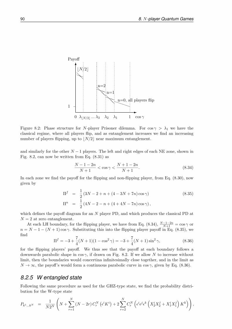
90 8. N -player Quantum Games
PP@@
PPP@@@
PPP@@@PPPP
-
6Payoff
cos γ0 1
1
λ1λ2λ3λ⌊N/2⌋ ...
⌊N/2⌋
n=2
n=1
n=0, all players flip
Figure 8.2: Phase structure for N -player Prisoner dilemma. For cos γ > λ1 we have theclassical regime, where all players flip, and as entanglement increases we find an increasingnumber of players flipping, up to ⌊N/2⌋ near maximum entanglement.
and similarly for the other N − 1 players. The left and right edges of each NE zone, shown inFig. 8.2, can now be written from Eq. (8.31) as
N − 1− 2n
N + 1< cos γ <
N + 1− 2n
N + 1. (8.34)
In each zone we find the payoff for the flipping and non-flipping player, from Eq. (8.30), nowgiven by
Πf =1
2(3N − 2 + n+ (4− 3N + 7n) cos γ) (8.35)
Πn =1
2(4N − 2− n+ (4 + 4N − 7n) cos γ) ,
which defines the payoff diagram for an N player PD, and which produces the classical PD atN = 2 at zero entanglement.
At each LH boundary, for the flipping player, we have from Eq. (8.34), N−1−2nN+1 = cos γ or
n = N − 1− (N + 1) cos γ. Substituting this into the flipping player payoff in Eq. (8.35), wefind
Πf = −3 + 7
4(N + 1)(1− cos2 γ) = −3 + 7
4(N + 1) sin2 γ, (8.36)
for the flipping players’ payoff. We thus see that the payoff at each boundary follows adownwards parabolic shape in cos γ, if drawn on Fig. 8.2. If we allow N to increase withoutlimit, then the boundaries would concertina infinitesimally close together, and in the limit asN →∞, the payoff’s would form a continuous parabolic curve in cos γ, given by Eq. (8.36).
8.2.5 W entangled state
Following the same procedure as used for the GHZ-type state, we find the probability distri-bution for the W-type state
Pk1...kN =1
N2N
(
N +N∑
r=1
(N − 2r)CNr(ǫiKi
)+ 2
N∑
r=2
CNr
(
ǫiǫjǫk(
Xi2X
j2 +Xi
1Xj1
)
Kk))
,

8.3 Conclusion 91
see Appendix B for derivation. We can then find the payoff function for the first player, Alice
ΠA(κ1, . . . , κN ) = Na0...0+
N∑
r=1
(N −2r)CNr (aiKi)+2N∑
r=2
CNr (aijk(Xi2X
j2 +X
i1X
j1)K
k) (8.37)
and similarly for other players.However with the W-type state it is impossible to turn off the entanglement, and so it will
not be possible to embed the classical game, as we have done with the GHZ-type state. Hencewe will not proceed any further except to show the result of maximizing the payoff functionin Eq. (8.37) for the Prisoner dilemma.
Prisoner Dilemma
For the Prisoner dilemma we can maximize the payoff function, and we find that we requireall players to flip, for all N and the resultant payoff for the first player Alice and hence allplayers is
ΠA = c+ d− c+ d− (a+ b)
N. (8.38)
So as N →∞, then the payoff approaches c+ d from below.
8.3 Conclusion
Using geometric algebra, the probability distribution is found after applying general measure-ment directions on a general N qubit entangled state, for the GHZ type Eq.(8.15) and Wstates Eq.(8.37).
Linear functions parameterized by the number of non-flipping players for an N player gameare then defined , from which games can then be defined in a general way. The linear functionsare solved for N players and the Nash equilibrium and payoff relations then determined.
As a specific example the Prisoner dilemma is solved for a general N and we find aninteresting feature, that the payoffs at the Nash equilibrium are equal for the flipping andnon-flipping player only for even N and also in the limit of large N the payoff rises linearlywith N given by (c+ a)N/4 for the GHZ type state.
At maximum entanglement the payoff for the GHZ type and W type states for the Prisonerdilemma become equal at N = 2, producing the formula
ΠGHZ = ΠW =a+ b+ c+ d
2. (8.39)
This equality is to be expected at N = 2, because these two states are equivalent up to localoperations.
So in summary we have produced a general quantum game environment, for any numberof players N ≥ 2, which will embed the classical game at zero entanglement, and usinglinear functions for player payoffs we can produce game outcomes for all N . Hence, the resultspreviously obtained for two-player and three-player games, are now subsumed by these results.
The linear functions could be generalized to second order to increase the range of gamesrepresented. For example, a quadratic term could be added to Eq. (8.24) to expand thevariety of games.

9
Conclusions
The research began with a general overview of the field of quantum computing, with the key el-ements and principles being outlined in chapter one. We then described the basic constructionof quantum computers from qubits using the circuit model framework for quantum computing,describing one qubit and two qubit gates, and some simple algorithms. We also introduced theformalism of Clifford geometric algebra which we proceeded to show in subsequent chapterscan be used as an alternative to the conventional bra-ket notation, and is particularly suitedto represent and describe rotations on qubits.
In chapter two we investigated the first of the two key algorithms of the field, Shor’sfactorization algorithm, followed by Grover’s search algorithm in chapter three.
Shor’s algorithm, is based on the operation of the phase estimation procedure, whichentails an associated probability of error. Several different estimates of this error have beenproduced in the literature, all requiring simplifying assumptions and approximations in orderto obtain a concise formula. A careful review of these derivations was carried out which notedan asymmetry in the definition of the error, which once corrected allowed an analytic solutionto be found [JMCL11b]. This formula will more easily allow the optimal design of quantumcomputers using the phase estimation procedure in the future.
The work on the error formula also motivated the development of a quantum computingsimulator, written in the Java programming language, to allow visual modeling of the keyalgorithms, which was extended over time to model most aspects of quantum computing.Using a graphical user interface, the program allowed the dragging of basic gates onto a circuitboard type layout, which allowed the sequential analysis of the wave function after each setof gates to be displayed. The software allowed a very clear visual picture of the operationof basic algorithms, and the software simulator could perhaps be utilized by students in thefuture to improve understanding of the basic operations of quantum computers.
In chapter three Grover’s search algorithm was investigated, and because it is knownthat the search process is an SU(2) rotation, we found a set of SU(2) generators for this space,based on the two non-orthogonal basis vectors |m〉 and |σ〉. This allowed us to identify theGrover search process as equivalent to the precession of the polarization axis of a spin-12 particlein a magnetic field. These results were presented on a poster at Quantum Information andControl in Queensland (QICIQ) and the 4th Asia Pacific Conference in Quantum InformationScience (4APCQIS) in 2008.
In chapter four The Grover search algorithm was then recast in the mathematical for-malism of GA (geometric algebra). This was done for two reasons, firstly because, as notedpreviously in chapter three, the Grover search process is an SU(2) rotation, and GA is knownto be a natural language in which to describe rotations, and secondly, because it providesa clear geometric picture within a real three dimensional space. We were then, for the firsttime, able to concisely reproduce the known results of the Grover search algorithm in thisformalism. We also found an efficient algebraic solution to the exact Grover search, and alsousing the visual picture provided by GA in three space, the more general search situationscould easily be understood in terms of different precession axes, or different locations in thespace of the starting and final states.
In chapter five we extended the use of qubits to the field of quantum game theory. Quan-tum games like quantum computers are based on application of unitary operations to qubits,and we apply the formalism of GA, successfully used for the Grover search, to describe Meyer’spenny flip game. This game is based on two players applying unitary operations to a single

94 9. Conclusions
common spin 12 particle. An analysis was completed, which enabled a general solution to be
found, along with a clear geometric picture describing the solution space [CILVS09](attached).
We then investigated quantum games from a more general perspective, representing gamesas a table of non-factorizable joint probabilities [CIA10]. This provides a natural link fromclassical probabilistic games to quantum games without recourse to the conventional quan-tum mechanical formalisms, thus making the field of quantum games more accessible to thenon-physicist. This approach provides a general framework within which both classical andquantum games can be located.
In chapter six and seven following the analysis of quantum games based on a singlequbit, it was then natural to extend this analysis to two-player and three-player and finally N -player quantum games, which differ from the Penny flip game in that each player is allocateda separate qubit from an entangled quantum state. Several different approaches, in fact, havebeen proposed in order to describe quantum games, but we chose a more recent approach,basing the quantum game on a physical EPR experiment. This approach has the advantageof avoiding a common criticism of quantum games, which states that quantum games aresimply different enhanced classical games. With the EPR approach, players choices remaincompletely classical, being simply the choice of two possible measurement directions, thusavoiding this criticism. We then investigated two-player and three-player games, with thethree-player game analysis being published in PLoS [JMCL11a], which was then extended toN -player games. The two-player and three-player games were both conducted in the samepattern in order to allow a straightforward generalization to the much more difficult N -playergames.
In chapter eight we extended the analysis of quantum games to the general N -playercase. For N players, clearly the use of matrices becomes unwieldy, but through describingunitary operations in GA and through writing the N×N payoff matrices in a functional form,we found that we could achieve general results as N →∞. We found for the Prisoner dilemmagame a new result could be found, that the payoffs at the Nash equilibrium are equal to eachother for the flipping and non-flipping player only for even N .
9.0.1 Original contributions
Several new results were obtained during the different investigations undertaken as part of mythesis, including four major results which were successfully published [JMCL11b, CILVS09,CIA10,JMCL11a].
The first new result achieved was the analytic solution to the problem of finding the errorlimits for the phase estimation procedure [JMCL11b], its significance being that this procedureis the basis for Shor’s factorization algorithm. Further investigations of the phase estimationprocedure then resulted in its novel application to performing the Grover search process inChapter 3.
The Grover search algorithm was then analyzed more generally, finding the three gener-ators of the SU(2) Grover search space, and finding an analogy of the search process withthe precession of a spin-12 particle in a magnetic field, which was presented on a poster atan international conference. The formalism of geometric algebra(GA) was then applied forthe first time to the analysis of the Grover search algorithm, which showed a very efficientdescription of this important algorithm, and due to its clarity may provide further insights.
The use of GA was then applied to an analogous situation involving the quantum pennyflip game, a game based on manipulating a single qubit, for which a general solution wasfound [CILVS09] and we showed that the use of GA also allowed a clear visual picture of thegeneral solution. Investigations in the field of quantum game theory continued which led to thedevelopment of a probabilistic framework for quantum games, which interprets entanglementas a classical non-factorizable joint probability distribution, and using a symmetric distributionwe found a very general framework within which to describe two-player games [CIA10].
95
As a special type of quantum game we then developed a quantum game frameworkbased on an EPR experiment, with general results for two-player, three-player and finallyN -player games achieved in Chapters 6 − 8, with three-player games being successfully pub-lished [JMCL11a] and two-player games currently submitted for peer review and N -playergames in preparation. This approach is significant as it has the advantage of avoiding a com-mon criticism of other quantum game frameworks of not properly embedding the underlyingclassical game.
As a more general product of the research we also showed how GA provides a suitableformalism for the whole field of quantum computing, and we found for example an efficientrepresentation for the Grover search in Chapter 4, and Shor’s factorization algorithm in Chap-ter 2 as well as the common gate operations shown in Chapter 1. Also, during this researcha quantum circuit simulation program was developed in the Java programming language,which allowed easy graphical analysis of the wavefunction for simple circuits, and which couldcontinue to be developed as an analysis tool.
9.0.2 Further work
We have presented the general equation for the Grover search in GA, but perhaps some specificcases could now be solved, such as more general starting states, and also the partial searchprocess could also perhaps be now placed within this framework.
The N -player formula could now be applied to specific game scenarios and perhaps manyspecific results could be forthcoming, such as investigating the common games of Stag hunt orMinority game, along with the optimal use of coalitions between players when more than twoplayers are involved. We have also defined N -player game payoffs using linear functions asopposed to a general N ×N payoff matrix, so that to achieve more generality, quadratic func-tions could now be employed to allow more general game definitions. Clearly these relationscould be expanded to arbitrary powers of n, in order to create more general games.
The use of a non-factorizable joint distribution in order to represent entanglement is infact a very generic approach, and if it could be extended to N participants it could be appliedin a general way to optimizing network performance, for example.
The Java simulator, which we developed, was a useful tool to test various ideas and tovisually see the resultant wave functions. This program could now be developed further as auseful learning tool for students wishing to gain a better understanding of the basic principlesof quantum computing algorithms.

A
Appendix
A.1 Actions of SU(2) generators on basis vectors
J1|σ〉 =−α∗
2|α| |m〉 =−e−iδ
2|m〉 (A.1)
J1|m〉 =−α2|α| |σ〉 =
−eiδ2|σ〉
J2|σ〉 =−iα∗
2|α|β |m〉+i|α|2β|σ〉 = −ie
−iδ
2β|m〉+ i|α|
2β|σ〉
J2|m〉 =−i|α|2β|m〉+ iα
2|α|β |σ〉 =−i|α|2β|m〉+ ieiδ
2β|σ〉
J3|σ〉 =1
2β(|σ〉 − α∗|m〉)
J3|m〉 =1
2β(α|σ〉 − |m〉)
J+|σ〉 =e−iδ(1− β)
2β|m〉 − |α|
2β|σ〉
J+|m〉 =−eiδ(1 + β)
2β|σ〉+ |α|
2β|m〉
J−|σ〉 =−e−iδ(1 + β)
2β|m〉+ |α|
2β|σ〉
J−|m〉 =eiδ(1− β)
2β|σ〉 − |α|
2β|m〉.
A.2 Euler angles in geometric algebra
Expanding a general rotor in the Euler angle form in terms of trigonometric functions, wehave
R = e−ισ3α2 e−ισ2
β2 e−ισ3
χ2 (A.2)
= cosβ
2cos
α+ χ
2+ sin
β
2sin
α− χ2
ισ1 − sinβ
2cos
α− χ2
ισ2 − cosβ
2sin
α+ χ
2ισ3.
We can now derive a few special cases:
Case 1: χ = −α:
R = e−ισ3α2 e−ισ2
β2 eισ3
α2 (A.3)
= cosβ
2+ sin
β
2sinαισ1 − sin
β
2cosαισ2
= eιβ2(sinασ1−cosασ2).

98 A. Appendix
Case 2: χ = α− π:
R = e−ισ3α2 e−ισ2
β2 e−ισ3
(α−π)2 (A.4)
= cosβ
2sinα+ sin
β
2ισ1 + cos
β
2cosαισ3
= eιb2(sin aσ1+cos aσ3),
where
tan a = tanβ
2secα (A.5)
cosb
2= cos
β
2sinα, (A.6)
or inverting the formulas we have
sinβ
2= sin a sin
b
2(A.7)
cotα = cos a tanb
2. (A.8)
Case 3:
R = eισ3α2 eισ2
β2 eισ3
α−π2 (A.9)
= cosβ
2sinα+ sin
β
2ισ1 − cos
β
2cosαισ3
= eιb2(sin aσ1−cos aσ3).
Case 4:
R = e−ισ3α2 eισ2
β2 eισ3
−α+π2 (A.10)
= cosβ
2sinα− sin
β
2ισ1 + cos
β
2cosαIσ3
= eιb2(− sin aσ1+cos aσ3).
A.3 Demonstration that the Grover oracle is a reflection about
m using GA
In the | ↑〉, | ↓〉 basis, a general state can be written
|ψ〉 =[− cos χ4sin χ
4
]
= − cosχ
4| ↑〉+ sin
χ
4| ↓〉. (A.11)
Writing the Grover oracle in this space, we have
Gm = I − 2|m〉〈m| = I − 2 sin2θ
4| ↑〉〈↑ |− 2 cos2
θ
4| ↓〉〈↓ |+sin
θ
2| ↑〉〈↓ |+sin
θ
2| ↓〉〈↑ |. (A.12)
We find
Gm|ψ〉 =
(
− cosχ
4+ 2 sin2
θ
4cos
χ
4+ sin
θ
2sin
χ
4
)
| ↑〉 (A.13)
+
(
sinχ
4− 2 cos2
θ
4sin
χ
4− sin
θ
2cos
χ
4
)
| ↓〉 (A.14)
= − cos
(θ
2+χ
4
)
| ↑〉 − sin
(θ
2+χ
4
)
| ↓〉 (A.15)
↔ − cos
(θ
2+χ
4
)
+ sin
(θ
2+χ
4
)
ισ2. (A.16)

A.4 Standard results when calculating observables 99
Using Eq.(4.6), we find
〈S〉 = sin(
θ +χ
2
)
σ1 + cos(
θ +χ
2
)
σ3. (A.17)
We see this new vector is then a reflection about the vector m.
A similar result holds for Gσ, that is
Gσ|ψ〉 ↔ − cos
(θ
2− χ
4
)
+ sin
(θ
2− χ
4
)
ισ2, (A.18)
which gives us
〈S〉 = sin(
θ − χ
2
)
σ1 + cos(
θ − χ
2
)
σ3, (A.19)
which once again is a simple reflection, but this time about σ.
A.4 Standard results when calculating observables
These results, particularly those shown in Eq. (A.25), are used when calculating the observ-ables in GA. We have also calculated the general case with general measurement directions inEq. (A.23). If we have a rotor defined as
A = e−α3ισ3/2e−α1ισ2/2e−α2ισ3/2 (A.20)
and for measurement, we use
R = e−λισ3/2e−κισ2/2e−ηισ3/2. (A.21)
We find, firstly
ιAσ1A† = ιe−α3ισ3/2e−α1ισ2/2e−α2ισ3/2σ1e
α2ισ3/2eα1ισ2/2eα3ισ3/2 (A.22)
= e−α3ισ3/2e−α1ισ2/2(cosα2 − sinα2ισ3)e−α1ισ2/2e−α3ισ3/2ισ1
= e−α3ισ3/2(cosα2e−α1ισ2 − sinα2ισ3)e
−α3ισ3/2ισ1
= e−α3ισ3/2(cosα2 cosα1 − cosα2 sinα1ισ2 − sinα2ισ3)e−α3ισ3/2ισ1
= (cosα1 cosα2e−α3ισ3 − sinα1 cosα2ισ2 − sinα2ισ3e
−α3ισ3)ισ1
= (cosα1 cosα2 cosα3 − cosα1 cosα2 sinα3ισ3 − sinα1 cosα2ισ2
− sinα2 cosα3ισ3 − sinα2 sinα3)ισ1
= (cosα1 cosα2 cosα3 − sinα2 sinα3)ισ1 − sinα1 cosα2ισ3
+(cosα1 cosα2 sinα3 + sinα2 cosα3)ισ2
ιAσ2A† = ιe−α3ισ3/2e−α1ισ2/2e−α2ισ3/2σ2e
α2ισ3/2eα1ισ2/2eα3ισ3/2
= e−α3ισ3/2e−α1ισ2/2(cosα2 − sinα2ισ3)eα1ισ2/2e−α3ισ3/2ισ2
= e−α3ισ3/2(cosα2 − sinα2ισ3eα1ισ2)e−α3ισ3/2ισ2
= e−α3ισ3/2(cosα2 − cosα1 sinα2ισ3 − sinα1 sinα2ισ1)e−α3ισ3/2ισ2
= (cosα2e−α3ισ3 − cosα1 sinα2ισ3e
−α3ισ3 − sinα1 sinα2ισ1)ισ2
= (cosα2 cosα3 − cosα1 sinα2 sinα3)ισ2 − (cosα2 sinα3 + cosα1 sinα2 cosα3)ισ1
+sinα1 sinα2ισ3
ιAσ3A† = cosα1ισ3 + sinα1 cosα3ισ1 + sinα1 sinα3ισ2,

100 A. Appendix
then we find the following results
〈ιAσ3A†ιRσ3R†〉0 = − cosα1 cosκ− sinα1 cosα3 sinκ cosλ (A.23)
− sinα1 sinα3 sinκ sinλ
= − cosα1 cosκ− cos(α3 − λ) sinα1 sinκ
〈ιAσ2A†ιRσ3R†〉0 = sinκ cosλ(cosα2 sinα3 + sinα2 cosα3 cosα1)− sinα1 sinα2 cosκ
− sinκ sinλ(cosα2 cosα3 − cosα1 sinα2 sinα3)
= − cosκ sinα1 sinα2 + sinκ(cosα1 cos(α3 − λ) sinα2
+cosα2 sin(α3 − λ))〈ιAσ1A†ιRσ3R
†〉0 = − sinκ cosλ(cosα1 cosα2 cosα3 − sinα2 sinα3) + sinα1 cosα2 cosκ
− sinκ sinλ(cosα1 cosα2 sinα3 + sinα2 cosα3)
= cosα2(cosκ sinα1 − cosα1 cos(α3 − λ) sinκ1)+ sinα2 sinκ sin(α3 − λ)
and also, we find
〈ιAσ1A†ιRσ1R†〉0 = − sinα1 cosα2 sinκ cos η (A.24)
− (cosα1 cosα2 sinα3 + sinα2 cosα3)(cosκ cos η sinλ+ sin η cosλ)
− (cosα1 cosα2 cosα3 − sinα2 sinα3)(cosκ cos η cosλ− sin η sinλ)
= sin(α3 − λ1)(cos η1 cosκ1 sinα2 − cosα1 cosα2 sin η1)
− cos(α3 − λ1)(cosα1 cosα2 cos η1 cosκ1 + sinα2 sin η
1)
− cosα2 cos η1 sinα1 sinκ
1
〈ιAσ2A†ιRσ2R†〉0 = − sinα1 sinα2 sinκ sin η
− (cosα2 sinα3 + cosα1 sinα2 cosα3)(cos η sinλ+ cosκ sin η cosλ)
− (cosα2 cosα3 − cosα1 sinα2 sinα3)(cos η cosλ− cosκ sin η sinλ)
= sin(α3 − λ1)(cosα1 cos η1 sinα2 − cosα2 cosκ
1 sin η1)
− cos(α3 − λ1)(cosα1 cosκ1 sinα2 sin η
1 + cosα2 cos η1)
− sinα1 sinα2 sin η1 sinκ1.
We have the special cases for just a single measurement direction κ
〈ιAσ3A†ισ3eκισ2〉0 = − cosα1 cosκ− sinα1 cosα3 sinκ (A.25)
〈ιAσ2A†ισ3eκισ2〉0 = sinκ(cosα2 sinα3 + sinα2 cosα3 cosα1)− sinα1 sinα2 cosκ
〈ιAσ1A†ισ3eκισ2〉0 = − sinκ(cosα1 cosα2 cosα3 − sinα2 sinα3) + sinα1 cosα2 cosκ.
A.5 Deriving the general two qubit state representation in GA
The Schmidt decomposition of a general two particle state can be written [DL03]
|ψ〉 = ρ12 eiχ
[
cosγ
2e
−iφ2
(
cosα1
2e
−iα32 |0〉+ sin
α1
2e
iα32 |1〉
)
⊗(
cosβ12e
−iβ32 |0〉+ sin
β12e
iβ32 |1〉
)
+ sinγ
2e
iφ2
(
sinα1
2e
−iα32 |0〉 − cos
α1
2e
iα32 |1〉
)
⊗(
sinβ12e
−iβ32 |0〉 − cos
β12e
iβ32 |1〉
)]
. (A.26)

A.5 Deriving the general two qubit state representation in GA 101
We note that the Schmidt decomposition assumes that cos γ ≥ sin γ, hence we need to enforcethe condition γ ∈ [0, π2 ]. Using the mapping defined in Eq. (1.24), we find that
e−iφ2
(
cosα1
2e
−iα32 |0〉+ sin
α1
2e
iα32 |1〉
)
= cosα1
2e
−i(φ+α3)2 |0〉+ sin
α1
2e
i(α3−φ2 |1〉
=
(
cosα1
2cos
φ+ α3
2− i cos
α1
2sin
φ+ α3
2
)
|0〉
+
(
sinα1
2cos
α3 − φ2
+ i sinα1
2sin
α3 − φ2
)
|1〉
→ cosα1
2cos
φ+ α3
2− cos
α1
2sin
φ+ α3
2ισ3
− sinα1
2cos
α3 − φ2
ισ2 + sinα1
2sin
α3 − φ2
ισ1
= e−ια3σ3/2e−ια1σ2/2e−ιφσ3/2. (A.27)
We can then also deduce that
eiχ(
cosβ12e
−iβ32 |0〉+ sin
β12e
iβ32 |1〉
)
→ e−ιβ3σ3/2e−ιβ1σ2/2eιχσ3 . (A.28)
If we then make the substitution α12 → −(π2 −
α12 ) we find
eiφ2
(
sinα1
2e
−iα32 |0〉 − cos
α1
2e
iα32 |1〉
)
→ −e−ια3σ3
2 eι(π2−α1
2)σ2e
ιφσ32
= −e−ια3σ3
2 e−ια1σ2
2 e−ιφσ3
2 ισ12, (A.29)
and
eiχ(
sinβ12e
−iβ32 |0〉 − cos
β12e
iβ32 |1〉
)
→ −e−ιβ3σ3
2 e−ιβ1σ2
2 ισ22eιχσ3 . (A.30)
The general state is then represented as
ψ = ρ12 e−ια3σ3/2e−ια1σ2/2e−ιφσ3/2e−ιβ3σ3/2e−ιβ1σ2/2(cos
γ
2+ sin
γ
2ισ12ισ
22)e
ιχσ3 . (A.31)
We notice the first qubit has an extra degree of freedom available in the applied rotor ascompared to the second qubit, namely, the parameter φ. However, we had a choice where weassociated the complex phase during the derivation. So if we split the phase eiφσ3/2 betweenthe two qubits as eiα2σ3/2 and eiβ2σ3/2, we can have symmetrical rotors on each qubit with
A = e−ια3σ3/2e−ια1σ2/2e−ια2σ3/2, B = e−ιβ3σ3/2e−ιβ1σ2/2e−ιβ2σ3/2, (A.32)
where φ = α2 + β2. The general two qubit state can now be written as
ψ = ρ12AB
(
cosγ
2+ sin
γ
2ισ12ισ
22
)
eιχσ3E. (A.33)
The extra E term on the end of the wave function is included because we have introduceda second copy of ι for the second particle space, whereas normally the complex number i iscommon across all particle spaces. We can remove this redundancy with a projection operator,E = 1
2(1 − ισ13ισ23). However, when we come to form the observables ψEψ† and ψJψ†, wenotice that because E2 = E and EJ = JE = J , we see that the inclusion of E, as well asthe global phase term eιχσ3 , will cancel out in both cases and hence is superfluous. Also fora pure state we have ρ = 1 and so without loss of generality, in regard to the observables, wecan write a general two-particle state in GA, compactly as
ψ = AB(
cosγ
2+ sin
γ
2ισ12ισ
22
)
. (A.34)
We see that with the five degrees of freedom provided with the rotors and also the entanglementangle γ, we have defined a two particle quantum state with six degrees of freedom, as requiredfor a normalized two-particle quantum state ignoring the global phase.

102 A. Appendix
A.6 Two-player games: SO6 geometric algebra
This approach is the most general method for two particles because it also allows a disentan-gling operation but, unfortunately, it cannot be generalized beyond two particles, because theisomorphism does not continue beyond SU(4).
We define two separate SO3 spaces e1, e2, e3 and f1, f2, f3 where e21 = f2i = 1 and all sixorthonormal vectors anti-commute with each other, and where we define
σ1i = eif1f2f3 = eiι2 (A.35)
σ2i = e1e2e3fi = ι1fi,
where the superscripts indicate which particle space the vector belongs to and let ι = ι1ι2,where we find ι1 and ι2 anti-commute, and so using this new combined ι, we find (ι)2 = ιι = −1.From now on ι will always refer to ι = e1e2e3f1f2f3, combined from both particle spaces. Thenwe find
σiσj = δij + ιǫijkσk, (A.36)
which mimics the Pauli algebra and
σ1i σ2j = σ2jσ
1i (A.37)
with its commuting property allows us to use the geometric product in the same way as thetensor product. We can identify a basis for two-particle spinor space as
|0〉|0〉 ←→ 1 (A.38)
|0〉|1〉 ←→ ισ22
|1〉|0〉 ←→ ισ12
|1〉|1〉 ←→ ισ12σ22.
In fact, for a general entangled two-particle state, we can write
ψ = A1B2(cosγ
2+ sin
γ
2ισ12σ
22), (A.39)
where γ is a measure of the entanglement, and A1 and B2 are general single particle ro-tors(unitary rotations) on each qubit.
General unitary operations in GA can be represented as
R(α1, α2, α3) = e−α3ισ3/2e−α1ισ2/2e−α2ισ3/2. (A.40)
This rotation, represented in geometric algebra, is in Euler angle form and can completelyexplore the available space of a single qubit, and is equivalent to the general unitary transfor-mation denoted by the matrix
[eiθ3/2 cos θ12 −e−iθ2/2 sin θ1
2
eiθ2/2 sin θ12 e−iθ3/2 cos θ12
]
(A.41)
acting on a spinor. We see that with the 3 degrees of freedom provided in each rotor and theentanglement angle γ, we have defined a two particle quantum state with 7 degrees of freedomas required for a two-particle quantum state ignoring the global phase.
The observables are found in geometric algebra from a density operator(which mimicdensity matrices) [PD01]
ρ = ψP 13P
23ψ
† (A.42)

A.6 Two-player games: SO6 geometric algebra 103
where P k3 = 1 + σk3 . So, we find
P 13P
23 = (1 + σ13)(1 + σ23) = (1 + σ13σ
23) + (σ13 + σ23). (A.43)
So, we have
ρ = ψP 13P
23ψ
† (A.44)
= ψ(1 + σ13 + σ23 + σ13σ23)ψ
†
= 1 + ψσ13σ23ψ
† + ψσ13ψ† + ψσ23ψ
†.
Taking each term from Eq.(A.44) in turn, starting with σ13, we find ψσ13ψ†
= AB(cosγ
2+ sin
γ
2ισ12σ
22)σ
13(cos
γ
2− sin
γ
2ισ12σ
22)B
†A† (A.45)
= AB(cosγ
2+ sin
γ
2ισ12σ
22)(cos
γ
2+ sin
γ
2ισ12σ
22)σ
13B
†A†
= AB(cos γ + sin γισ12σ22)σ
13B
†A†
= cos γAσ13A† − sin γAσ11A
†Bσ22B†,
where we used the results σ13σ12 = −σ12σ13, ισ12σ22ισ12σ22 = ι2 = −1 and ισ12σ
22σ
13 = −σ11σ22. By
symmetry of the first and second particle, we can immediately write
ψσ23ψ† = cos γBσ23B
† − sin γAσ12A†Bσ21B
†. (A.46)
Finally, we have ψσ13σ23ψ
†
= AB(cosγ
2+ sin
γ
2ισ12σ
22)σ
13σ
23(cos
γ
2− sin
γ
2ισ12σ
22)B
†A† (A.47)
= AB(cosγ
2+ sin
γ
2ισ12σ
22)(cos
γ
2− sin
γ
2ισ12σ
22)σ
13σ
23B
†A†
= ABσ13σ23B
†A†
= Aσ13A†Bσ23B
†.
So, the full density operator is
ρ = 1 + cos γAσ13A† − sin γAσ11A
†Bσ22B† (A.48)
+ cos γBσ23B† − sin γAσ12A
†Bσ21B† +Aσ13A
†Bσ23B†
= 1 + cos γ(Aσ13A† +Bσ23B
†)
+ Aσ13A†Bσ23B
† − sin γ(Aσ11A†Bσ22B
† +Aσ12A†Bσ21B
†).
For measurement, we employ the density operator
ρM = R1R2(1 + σ13 + σ23 + σ13σ23)R
1R2 (A.49)
and we have R1 = eικ1σ1
2 and R2 = eικ2σ2
2 where κ1 and κ2 are measurement directions forplayers 1 and 2 respectively, so that we have
ρM = eικσ12/2eικσ
22/2(1 + σ13 + σ23 + σ13σ
23)e
−ικσ22/2e−ικσ
12/2 (A.50)
= 1 + σ13e−ικσ1
2 + σ23e−ικσ1
2 + σ13σ23e
−ικσ22e−ικ2σ2 .
104 A. Appendix
Retaining the scalar part of the product ρMρ, written as 〈ρMρ〉0 , we find the probability ofmeasuring each wave state as
4Pmn = 〈ρMρ〉0 (A.51)
= 〈[1 + cos γ(Aσ13A† +Bσ23B
†)
+ Aσ13A†Bσ23B
† − sin γ(Aσ11A†Bσ22B
† +Aσ12A†Bσ21B
†)]
× [1 + σ13e−ικ1σ1
2 + σ23e−ικ2σ2
2 + σ13σ23e
−ικ1σ12e−ικ
2σ22 ]〉0
= 〈1 + cos γ(Aσ13A†σ13e
−ικ1σ12 +Bσ23B
†σ23)e−ικ2σ2
2
+ Aσ13A†σ13Bσ
23B
†σ23e−ικ1σ1
2e−ικ2σ2
2
− sin γ(Aσ11A†σ13Bσ
22B
†σ23 +Aσ12A†σ13Bσ
21B
†σ23)e−ικ1σ1
2e−ικ2σ2
2 〉0= 1 + cos γ((−)mA+ (−)nB + (−)m+nAB + (−)m+n sin γZ,
where
A(κ1) = cosα1 cosκ1 − sinα1 cosα3 sinκ
1 (A.52)
B(κ2) = cosβ1 cosκ2 − sinβ1 cosβ3 sinκ
2
and
Z(κ1, κ2) = (cos k1 sinα1 + cosα1 cosα3 sinκ1) (A.53)
×(cosκ2 sinβ1 sinφ+ sinκ2 sinβ3 cosφ+ sinκ2 cosβ1 cosβ3 sinφ)
− sinκ1 sinκ2 sinβ3 sinα3 sinφ+ cosκ2 sinβ1 cosφ sinα3 sinκ1
+ sinκ2 cosβ1 cosβ3 cosφ sinα3 sinκ1.
To simplify notation, we will write Zij = Z(κ1i , κ2j ) , Ai = A(κ1i ) and Bj = B(κ2j ), where
i, j ∈ 1, 2 represent the two possible measurement directions available to each player. Wenotice that we still have some symmetry in our result because we have made the substitutionφ = α2 + β2 , so that we have six degrees of freedom out of a possible seven. This finalsymmetry would probably be lost if we allow variations of measurement directions out of theplane perpendicular to the line of sight.
If we try γ = 0 for no entanglement, we have the probability
Pmn =1
4(1 + (−)mA+ (−)nB (A.54)
+(−)m+nAB)
=(1 + (−)mA)1
2
(1 + (−)nB)2
2,
which shows a product state incorporating general measurement directions for each qubit.Writing out the probabilities for the four measurement outcomes with general measurement
directions, we find
P00(κ1, κ2) =
1
4[1 + cos γ(A(κ1) +B(κ2)) + (A(κ1)B(κ2) + sin γZ(κ1, κ2))] (A.55)
P01(κ1, κ2) =
1
4[1 + cos γ(A(κ1)−B(κ2))− (A(κ1)B(κ2) + sin γZ(κ1, κ2))]
P10(κ1, κ2) =
1
4[1 + cos γ(−A(κ1) +B(κ2))− (A(κ1)B(κ2) + sin γZ(κ1, κ2))]
P11(κ1, κ2) =
1
4[1 + cos γ(−A(κ1)−B(κ2)) + (A(κ1)B(κ2) + sin γZ(κ1, κ2))].
We allow each player the classical probabilistic choice between the two allocated measurementdirections for their Stern-Gerlach detectors. The two players choose their first measurement

A.6 Two-player games: SO6 geometric algebra 105
direction with probability x and y respectively, where x, y ∈ [0, 1]. We will assume the generalcase where players can choose different measurement directions to each other.
Now, we have the mathematical expectation of Alices’ payoff where she chooses the direc-tion κ11 with probability x and the measurement direction κ12 with probability 1− x as
ΠA(x, y) = xy(P00(κ11, κ
21)G00 + P01(κ
11, κ
21)G01 + P10(κ
11, κ
21)G10 + P11(κ
11, κ
21)G11) (A.56)
+ x(1− y)(P00(κ11, κ
22)G00 + P01(κ
11, κ
22)G01 + P10(κ
11, κ
22)G10 + P11(κ
11, κ
22)G11)
+ y(1− x)(P00(κ12, κ
21)G00 + P01(κ
12, κ
21)G01 + P10(κ
12, κ
21)G10 + P11(κ
12, κ
21)G11)
+ (1− x)(1− y)(P00(κ12, κ
22)G00 + P01(κ
12, κ
22)G01 + P10(κ
12, κ
22)G10 + P11(κ
12, κ
22)G11),
where, for the Prisoner dilemma, we have
GAij =
[3 05 1
]
=
[G00 G01
G10 G11
]
=
[K LM N
]
. (A.57)
For symmetric games, such as the Prisoner dilemma game, we have GBij = GAji. Generallyspeaking, any payoff matrix satisfying G10 > G00 > G11 > G01 is in the form of a Prisonerdilemma.
In the classical Prisoner dilemma game, we have two prisoners Alice and Bob being heldin separate cells ready to be interviewed. To encourage confessions, the interrogator sets outa reward scheme, where if the players qubit is measured as the |0〉 state, then this correspondsto exonerating the other prisoner(co-operating with the other prisoner) and |1〉 corresponds toaccusing the other prisoner(defection), which allows four possible payoff results, as shown in thepayoff matrix. So, if Alice co-operates but Bob defects against her, for example, Alice receivesa reward of 0, and Bob receives a payoff of 5 units. This game forms a dilemma for both playersbecause there is a conflict between the maximum payout received by two rational responsesbased on satisfying self interest(called the Nash equilibrium), and the Pareto optimum, whichis the best overall payoff available to both players. The Nash equilibrium will be both playersdefecting and receiving 1 unit in this case, because we can see that if either player decides tochange their choice from this position they will receive a smaller payoff of 0. If both playersthough could trust each other and co-operate they would both receive a greater payout of 3units, however there is a great temptation for either player to break the agreement and defectand improve his payoff to 5. We find that this impasse appears to be partially solved throughthe use of entanglement in the quantum form of the game.
We also define ∆1 = G10−G00, ∆2 = G11−G01 and ∆3 = ∆2−∆1 . We have ∆1,∆2 > 0for the Prisoner dilemma game in general. We define
p =1
4[(A1 −A2)(B1 −B2) + sin γ(Z11 + Z22 − Z12 − Z21)] (A.58)
so that we find the payoff for Alice
ΠA(x, y) =1
4[G00 +G10 +G01 +G11 (A.59)
+ ∆34pxy + x((A1 −A2)B2 + (Z12 − Z22) sin γ) + y((B1 −B2)A2 + (Z21 − Z22) sin γ)
+ A2B2 + Z22 sin γ − cos γ(∆1 +∆2)((A1 −A2)x+A2)
+ cos γ(G00 −G01 +G10 −G11)((B1 −B2)y +B2)].
A.6.1 Solving the two-player game
To find the Nash equilibrium, we require
ΠA(x∗, y∗) ≥ ΠA(x, y
∗) (A.60)
ΠB(x∗, y∗) ≥ ΠB(x
∗, y)
106 A. Appendix
which is stating that any movement of a player away from the Nash equilibrium (x∗, y∗), willresult in a lower payoff for that player. We find
ΠA(x∗, y∗)−ΠA(x, y
∗) (A.61)
=1
4(x∗ − x)[∆34py∗ + (A1 −A2)B2 + (Z12 − Z22) sin γ − cos γ(∆1 +∆2)(A1 −A2)]
=1
4(x∗ − x)(A1 −A2)[∆3y∗(B1 +
sin γ(Z11 − Z21)
A1 −A2) + (1− y∗)(B2 +
sin γ(Z12 − Z22)
A1 −A2)
− cos γ(∆1 +∆2)]
and for the second player Bob we have similarly
ΠB(x∗, y∗)−ΠB(x
∗, y) (A.62)
=1
4(y∗ − y)[∆34px∗ + (B1 −B2)A2 + (Z21 − Z22) sin γ − cos γ(∆1 +∆2)(B1 −B2)].
A.6.2 Embedding the classical game
We would like the classical game embedded in the quantum game at zero entanglement(γ = 0),and so the requirement for a N.E. becomes
ΠA(x∗, y∗)−ΠA(x, y
∗) (A.63)
=1
4(x∗ − x)(A1 −A2)[∆3y∗B1 + (1− y∗)B2 − (∆1 +∆2)] ≥ 0.
Because |∆3| ≤ |∆1 +∆2|, the term in square brackets is always negative and if A1 −A2 > 0,then we have the classical NE (x∗ = 0). By symmetry, Bob also has the NE y∗ = 0, providedB1−B2 > 0. At this NE of (x∗, y∗) = (0, 0) and at zero entanglement we find the payoff fromEq. (A.59) to be
ΠA(x, y) =1
4[G00(1 +A2)(1 +B2) +G10(1−A2)(1 +B2) (A.64)
+G01(1 +A2)(1−B2) +G11(1−A2)(1−B2)].
In order to achieve the classical payoff of G11, we can see that we require A2 = −1 andB2 = −1, that is
A(κ12) = cosα1 cosκ12 − sinα1 cosα3 sinκ
12 = −1 (A.65)
B(κ22) = cosβ1 cosκ22 − sinβ1 cosβ3 sinκ
22 = −1.
These equations have two classes of solution: if α3, β3 6= 0, then we have for the first equationα1 = 0, κ12 = π or α1 = π, κ12 = 0 and similarly for the second equation. For the second classwith α3, β3 = 0, we have the solution α1 + κ12 = π and β1 + κ22 = π.
For the first class, we find Z22 = Z21 = Z12 = 0 and Z11 = sinκ11 sinκ21 sin(α3+β3+α2+β2)
and for the second class, we find Z22 = Z21 = Z12 = 0 and Z11 = sin(α1 + κ11) sin(β1 +κ21) sin(α2 + β2).
These two classes gives the NE, governed in both cases
ΠA(x∗, y∗)−ΠA(x, y
∗) (A.66)
=1
4(x∗ − x)(cosκ11 + 1)[∆3y∗(cosκ21 +
sin γZ11
cosκ11 + 1)− (1− y∗) − cos γ(∆1 +∆2)] ≥ 0
with a corresponding payoff of
ΠA(x, y) =1
4[2(G00 +G11)− 2 cos γ(G00 −G11) (A.67)
+ xy∆3(A1 + 1)(B1 + 1) + sin γZ11 − x(A1 + 1)∆3 + cos γ(∆1 +∆2)−y(B1 + 1)∆3 − cos γ(G00 −G01 +G10 −G11)].
Thus Eq. (A.66) governs the possible NE and Eq. (A.67) the associated payoffs for a quantumPrisoner dilemma game which will embed the classical game at zero entanglement.

A.7 Two-player games: entangled measurement model 107
A.7 Two-player games: entangled measurement model
In this approach we have a local realist model consisting of two unentangled qubits uponwhich Alice and Bob act with their local unitary transformations. We then measure using aBell type measurement operator, placing all non-local correlations in the final measurementoperator. The advantage is, that we can easily visualize the state of the two separate qubitsas two separate Bloch sphere vectors.
We use the same basis as Alternative Method 1 two-particle spinor space as
|0〉|0〉 ←→ 1 (A.68)
|0〉|1〉 ←→ −ισ22|1〉|0〉 ←→ −ισ12|1〉|1〉 ←→ ισ12ισ
22.
We assume a separable state is prepared for Alice and Bob upon which they act producing,
ψ = AB (A.69)
where
A = R(α1, α2, α3) (A.70)
B = R(β1, β2, β3).
We have the two observables ψJψ† and ψEψ†, where
J = ισ13 + ισ23 (A.71)
E = 1− ισ13ισ23.
Given a measurement operator
φ = eικσ12/2eικσ
22/2(cos γ + sin γισ12ισ
22) (A.72)
to represent the measurement, where γ ∈ [−π2 ,
π2 ], and κ = 0, π for the measurement direction.
We are using the notation κσ22 = κ2σ22, so we can have separate κ for each particle space. Soforming the observables we have
ψJψ† = AB(ισ13 + ισ23)A†B† (A.73)
=1
2(ιAσ13A
† + ιBσ23B†)
and for the joint observable
ψEψ† = AB(1− ισ13ισ23)A†B† (A.74)
=1
2
(
1− ιAσ13A†ιBσ23B†)
and for the measurement settings
φJφ† = eικσ12/2eικσ
22/2(cos
γ
2+ sin
γ
2ισ12ισ
22)(ισ
13 + ισ23) (A.75)
× (cosγ
2+ sin
γ
2ισ12ισ
22)e
−ικσ22/2e−ικσ
22/2
=1
2eικσ
12/2eικσ
22/2(cos2
γ
2− sin2
γ
2)
× (ισ13 + ισ23)eικσ2
2/2e−ικσ12/2
=1
2cos γ(eικσ
12 ισ13 + eικσ
22 ισ23)

108 A. Appendix
φEφ† = eικσ12/2eικσ
22/2(cos
γ
2+ sin
γ
2ισ12ισ
22)(1− ισ13ισ23) (A.76)
× (cosγ
2+ sin
γ
2ισ12ισ
22)e
−κσ22/2e−κσ
12/2
=1
2(1− ιeικσ1
2eικσ22σ13ισ
23 + sin γ(ισ12ισ
22 − ιeικσ
12eικσ
22σ11ισ
21)),
from which we can calculate the probabilities to measure different states. For the special casesκ = 0, π, which defines the standard measurement basis, we have
φJφ† =1
2cos γ((−)xισ13 + (−)yισ23),
where each x, y ∈ 0, 1 refers to measuring a |0〉 or a |1〉 state, respectively and
φEφ† = −1
2
(1 + (−)x+yισ13ισ23 + sin γ(ισ12ισ
22 + (−)x+yισ11ισ21)
).
So, the separable part of the measurement is
= −〈ψJψ†φJφ†〉 (A.77)
= −1
2(ιAσ13A
† + ιBσ23B†)1
2cos γ((−)xισ13 + (−)yισ23)
=1
4cos γ((−)x cosα1 + (−)y cosβ1).
For the joint measurement
= 〈ψEψ†φEφ†〉 (A.78)
= −1
4(1− ιAσ13A†ιBσ23B
†)
×(1 + (−)x+yισ13ισ23 + sin γ(ισ12ισ
22 + (−)x+yισ11ισ21)
)
=1
4(1 + (−)x+y cosα1 cosβ1 − sin γ sinα1 sinα2 sinβ1 sinβ2
+ (−)x+y sin γ sinα1 cosα2 sinβ1 cosβ2)
=1
4(1 + (−)x+y cosα1 cosβ1 + (−)x+y sin γ sinα1 sinβ1 cos(α2 − (−)x+yβ2).
So, the final density operator is
ρ =1
4(1 + cos γ((−)x cosα1 + (−)y cosβ1) (A.79)
+ (−)x+y cosα1 cosβ1 + (−)x+y sin γ sinα1 sinβ1 cos(α2 − (−)x+yβ2)).
So, we can generate the four probabilities
P00 =1
4(1 + cosα1 cosβ1 + cos γ(cosα1 + cosβ1) (A.80)
+ sin γ sinα1 sinβ1 cos(α2 − β2))
P01 =1
4(1− cosα1 cosβ1 + cos γ(cosα1 − cosβ1)
− sin γ sinα1 sinβ1 cos(α2 + β2))
P10 =1
4(1− cosα1 cosβ1 + cos γ(− cosα1 + cosβ1)
− sin γ sinα1 sinβ1 cos(α2 + β2))
P11 =1
4(1 + cosα1 cosβ1 − cos γ(cosα1 + cosβ1)
+ sin γ sinα1 sinβ1 cos(α2 − β2)).
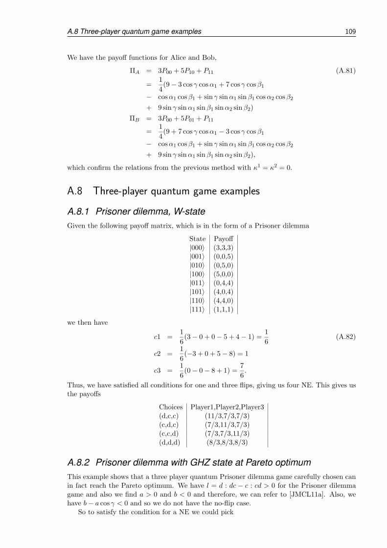
A.8 Three-player quantum game examples 109
We have the payoff functions for Alice and Bob,
ΠA = 3P00 + 5P10 + P11 (A.81)
=1
4(9− 3 cos γ cosα1 + 7 cos γ cosβ1
− cosα1 cosβ1 + sin γ sinα1 sinβ1 cosα2 cosβ2
+ 9 sin γ sinα1 sinβ1 sinα2 sinβ2)
ΠB = 3P00 + 5P01 + P11
=1
4(9 + 7 cos γ cosα1 − 3 cos γ cosβ1
− cosα1 cosβ1 + sin γ sinα1 sinβ1 cosα2 cosβ2
+ 9 sin γ sinα1 sinβ1 sinα2 sinβ2),
which confirm the relations from the previous method with κ1 = κ2 = 0.
A.8 Three-player quantum game examples
A.8.1 Prisoner dilemma, W-state
Given the following payoff matrix, which is in the form of a Prisoner dilemma
State Payoff|000〉 (3,3,3)|001〉 (0,0,5)|010〉 (0,5,0)|100〉 (5,0,0)|011〉 (0,4,4)|101〉 (4,0,4)|110〉 (4,4,0)|111〉 (1,1,1)
we then have
c1 =1
6(3− 0 + 0− 5 + 4− 1) =
1
6(A.82)
c2 =1
6(−3 + 0 + 5− 8) = 1
c3 =1
6(0− 0− 8 + 1) =
7
6.
Thus, we have satisfied all conditions for one and three flips, giving us four NE. This gives usthe payoffs
Choices Player1,Player2,Player3(d,c,c) (11/3,7/3,7/3)(c,d,c) (7/3,11/3,7/3)(c,c,d) (7/3,7/3,11/3)(d,d,d) (8/3,8/3,8/3)
A.8.2 Prisoner dilemma with GHZ state at Pareto optimum
This example shows that a three player quantum Prisoner dilemma game carefully chosen canin fact reach the Pareto optimum. We have l = d : dc − c : cd > 0 for the Prisoner dilemmagame and also we find a > 0 and b < 0 and therefore, we can refer to [JMCL11a]. Also, wehave b− a cos γ < 0 and so we do not have the no-flip case.
So to satisfy the condition for a NE we could pick

110 A. Appendix
State Payoff|000〉 (6,6,6)|001〉 (3,3,12)|010〉 (3,12,3)|100〉 (12,3,3)|011〉 (0,9,9)|101〉 (9,0,9)|110〉 (9,9,0)|111〉 (1,1,1)
We have c : cc = 6, c : cd = 3, d : cc = 12, c : dd = 0, d : dc = 9, d : dd = 1, givingus m = d : cc − c : cc = 12 − 6 = 6 and n = d : dd − c : dd = 1 − 0 = 1, giving usa = n + m = 7 and b = n − m = −5, and so b/a < 0, so we have the first case. Also, wehave l = d : dc − c : cd = 9 − 3 > 0 and so no single flip NE exist. We have a transition atcos γ = 5/7 from a quantum to a classical region and the maximum payoff at cos γ = 0 fornot flipping
Πf =1
2(0 + 12) = 6 (A.83)
Πn =1
2(3 + 9) = 6,
so that, at maximum entanglement, we reach the Pareto optimum as a Nash equilibrium.Classically, the NE is at 1.
A.9 W entangled state
We have the state before measurement from Eq.(8.4) as
ψ = − 1√N
(∏
U i) N∑
i
ιei2. (A.84)
So forming the observables from Eq.(1.25) we have
ψJψ† (A.85)
= − 1
N2N−1
(∏
U i) N∑
i
ιei2
N+12∑
r=1
(−)r+1CN2r−1(ιei3)
N∑
i
ιei2
(∏
U i†)
=1
N2N−1
(∏
U i)( (N+1)/2
∑
r=1
(N − 4r + 2)CN2r−1(ιei3)− 2
(N−1)/2∑
r=1
CN2r+1(ιei2ιe
j2ιe
k3)
− 2
(N−1)/2∑
r=1
CN2r+1(ιei1ιe
j1ιe
k3))(∏
U i†)
=1
N2N−1
( (N+1)/2∑
r=1
(−)r+1(N − 4r + 2)CN2r−1(Vi3 ) + 2
(N−1)/2∑
r=1
(−)rCN2r+1(Vi2V
j2 V
k3 )
+ 2
(N−1)/2∑
r=1
(−)rCN2r+1(Vi1V
j1 V
k3 ))
,

A.9 W entangled state 111
where V ik = ιU iekU
i† . Also from Eq.(1.25) we have
ψEψ† (A.86)
= − 1
N2N−1
(∏
U i) N∑
i
ιei2
1 +
N/2∑
r=1
(−)rCN2r(ιei3)
N∑
i
ιei2
(∏
U i†)
=1
N2N−1
∏
U i(
N − 2
N/2∑
r=1
CN2r(ιei2ιe
j2ιe
k3) +
N/2∑
r=1
(4r −N)CN2r(ιei3)
− 2
N/2∑
r=1
CN2r(ιei1ιe
j1ιe
k3))∏
U i†
=1
N2N−1
(
N + 2
N/2∑
r=1
(−)rCN2r(V i2V
j2 V
k3 ) +
N/2∑
n=1
(−)r(N − 4r)CN2r(Vi3 )
+ 2
N/2∑
r=1
(−)rCN2r(V i1V
j1 V
k3 ))
.
So, referring to Eq.(1.25), we find
−2N−2〈ψJψ†φJφ†〉0 (A.87)
= − 1
N2N
⟨( (N+1)/2∑
r=1
(−)r+1(N − 4r + 2)CN2r−1(Vi3 ) + 2
(N−1)/2∑
r=1
(−)rCN2r+1(Vi2V
j2 V
k3 )
+ 2
(N−1)/2∑
r=1
(−)rCN2r+1(Vi1V
j1 V
k3 ))(
N+12∑
r=1
(−)r+1CN2r−1(ιei3eικei2)
)⟩
0
=1
N2N
N+12∑
r=1
(N − 4r + 2)CN2r−1(Ki) + 2
N−12∑
r=1
CN2r+1(Xi2X
j2K
k) + 2
N−12∑
r=1
CN2r+1(Xi1X
j1K
k)
=1
N2N
N+12∑
r=1
(N − 4r + 2)CN2r−1(Ki) + 2
N−12∑
r=1
CN2r+1
(
(Xi2X
j2 +Xi
1Xj1)X
k3
)
.
Also from Eq.(1.25), we find
2N−2〈ψEψ†φEφ†〉0 (A.88)
=1
N2N
⟨(
N + 2
N/2∑
r=1
(−)rCN2r(V i2V
j2 V
k3 ) +
N/2∑
r=1
(−)r(N − 4r)CN2r(Vi3 )
+ 2
N/2∑
r=1
(−)rCN2r(V i1V
j1 V
k3 ))(
1 +
N/2∑
r=1
(−)rCN2r(ιei3eικei2))⟩
0
=1
N2N(N + 2
N/2∑
r=1
CN2r(ǫiǫjXi
2Xj2X
k3 ) +
N/2∑
r=1
(N − 4r)CN2r(Ki)
+2
N/2∑
r=1
CN2r(ǫiǫjǫkXi
1Xj1X
k3 ))
=1
N2N
N +
N/2∑
r=1
(N − 4r)CN2r(Ki) + 2
N/2∑
r=1
CN2r((Xi
2Xj2 +Xi
1Xj1)K
k)
.

112 A. Appendix
So the probabilities that a measurement will return a given state will be
Pk1...kN =1
N2N
( (N+1)/2∑
r=1
(N − 4r + 2)CN2r−1(Ki) + 2
(N−1)/2∑
r=1
CN2r+1
((Xi
2Xj2 +Xi
1Xj1)K
k)
+ N +
N/2∑
r=1
(N − 4r)CN2r(Ki)+ 2
N/2∑
r=1
CN2r((Xi
2Xj2 +Xi
1Xj1)K
k))
and combining the summation terms we find the probability distribution, for the W-type statesubject to general measurement directions
Pk1...kN =1
N2N
(
N +N∑
r=1
(N − 2r)CNr(ǫiKi
)+ 2
N∑
r=2
CNr(ǫiǫjǫk(Xi
2Xj2 +Xi
1Xj1)K
k)
)
.

Bibliography
[ADR82] A. Aspect, J. Dalibard, and G. Roger. Experimental test of Bell’s inequalities using time-varyinganalyzers. Physical Review Letters, 49(25):1804–1807, 1982.
[AR10] H. Anton and C. Rorres. Elementary linear algebra: applications version. Wiley, 2010.
[AS64] M. Abramowitz and I.A. Stegun. Handbook of mathematical functions with formulas, graphs, andmathematical tables. Dover publications, New York, 1964.
[AV08] N. Aharon and L. Vaidman. Quantum advantages in classically defined tasks. Physical Review A,77(5):052310, 2008.
[B+64] J.S. Bell et al. On the Einstein-Podolsky-Rosen paradox. Physics, 1(3):195–200, 1964.
[BBB+99a] E. Biham, O. Biham, D. Biron, M. Grassl, and D.A. Lidar. Grovers quantum search algorithm foran arbitrary initial amplitude distribution. Physical Review A, 60(4):2742, 1999.
[BBB+99b] D. Biron, O. Biham, E. Biham, M. Grassl, and D. Lidar. Generalized Grover search algorithmfor arbitrary initial amplitude distribution. Quantum Computing and Quantum Communications,pages 140–147, 1999.
[BBB+00] E. Biham, O. Biham, D. Biron, M. Grassl, D.A. Lidar, and D. Shapira. Analysis of generalizedGrover quantum search algorithms using recursion equations. Physical Review A, 63(1):012310,2000.
[BBBV97] E. Bernstein, C. Bennett, G. Brassard, and U. Vazirani. Strengths and weaknesses of quantumcomputing. SIAM J. Computing, 26:1510–1523, 1997.
[BBHT98] M. Boyer, G. Brassard, P. Høyer, and A. Tappa. Tight bounds on quantum searching. Fortschritteder Physik, 46:493–506, 1998.
[Bel66] J.S. Bell. On the problem of hidden variables in quantum mechanics. Reviews of Modern Physics,38(3):447–452, 1966.
[Bel87] JS Bell. Speakable and Unspeakable in Quantum Mechanics. Cambridge Univ. Press, 1987.
[BH01] S.C. Benjamin and P.M. Hayden. Multiplayer quantum games. Physical Review A, 64(3):030301,2001.
[Bin07] K.G. Binmore. Game theory: a very short introduction, volume 173. Oxford University Press,USA, 2007.
[BJ] P. Blanchard and A. Jadczyk. Quantum future. Springer-Verlag.
[BK02a] J. Bae and Y. Kwon. Generalized quantum search hamiltonian. Physical Review A, 66(1):012314,2002.
[BK02b] E. Biham and D. Kenigsberg. Grovers quantum search algorithm for an arbitrary initial mixedstate. Physical Review A, 66(6):062301, 2002.
[Bla80] A. Blaquiere. Wave mechanics as a two-player game. Dynamical Systems and Microphysics, 33,1980.
[Boh51] D. Bohm. Quantum theory. Dover Publications, 1951.
[CEMM98] R. Cleve, A. Ekert, C. Macchiavello, and M. Mosca. Quantum algorithms revisited. Proceed-ings of the Royal Society of London. Series A: Mathematical, Physical and Engineering Sciences,454(1969):339, 1998.
[Cer00] J.L. Cereceda. Quantum mechanical probabilities and general probabilistic constraints forEinstein–Podolsky–Rosen–Bohm experiments. Foundations of Physics Letters, 13(5):427–442,2000.
[CH01] A. Carlini and A. Hosoya. Quantum computers and unstructured search: finding and countingitems with an arbitrarily entangled initial state. Physics Letters A, 280(3):114–120, 2001.
[Chr07] J. Christian. Disproof of Bell’s theorem by Clifford algebra valued local variables. Arxiv preprintquant-ph/0703179, 2007.
[CIA10] J.M. Chappell, A. Iqbal, and D. Abbott. Constructing quantum games from symmetric non-factorizable joint probabilities. Physics Letters A, 374, 2010.
[CILVS09] J.M. Chappell, A. Iqbal, M.A. Lohe, and L. Von Smekal. An analysis of the quantum penny flipgame using geometric algebra. Journal of the Physical Society of Japan, 78(5):4801, 2009.

114 BIBLIOGRAPHY
[Cli78] W.K. Clifford. Applications of grassmann’s extensive algebra. American Journal of Mathematics,1(4):350–358, 1878.
[CS78] J.F. Clauser and A. Shimony. Bell’s theorem. experimental tests and implications. Reports onProgress in Physics, 41:1881, 1978.
[CT06] T. Cheon and I. Tsutsui. Classical and quantum contents of solvable game theory on hilbert space.Physics Letters A, 348(3-6):147–152, 2006.
[CvD10] A.M. Childs and W. van Dam. Quantum algorithms for algebraic problems. Reviews of ModernPhysics, 82(1):1, 2010.
[CZ95] J.I. Cirac and P. Zoller. Quantum computations with cold trapped ions. Physical Review Letters,74(20):4091–4094, 1995.
[Daw76] R. Dawkins. The selfish gene. Oxford University Press, USA, 1976.
[DDL02] L. Dorst, C.J.L. Doran, and J. Lasenby. Applications of geometric algebra in computer science andengineering. Birkhauser, Boston, 2002.
[Deu85] D. Deutsch. Quantum theory, the Church-Turing principle and the universal quantum computer.Proceedings of the Royal Society of London. A. Mathematical and Physical Sciences, 400(1818):97,1985.
[DKK03] S. Das, R. Kobes, and G. Kunstatter. Energy and efficiency of adiabatic quantum search algo-rithms. Journal of Physics A: Mathematical and General, 36:2839, 2003.
[DL03] C.J.L. Doran and A.N. Lasenby. Geometric algebra for physicists. Cambridge Univ Pr, 2003.
[DLX+02a] J. Du, H. Li, X. Xu, M. Shi, J. Wu, X. Zhou, and R. Han. Experimental realization of quantumgames on a quantum computer. Physical Review Letters, 88(13):137902, 2002.
[DLX+02b] J. Du, H. Li, X. Xu, X. Zhou, and R. Han. Entanglement enhanced multiplayer quantum games.Physics Letters A, 302(5-6):229–233, 2002.
[DSD07] V. De Sabbata and B.K. Datta. Geometric algebra and applications to physics. Taylor & FrancisGroup, 2007.
[dSR08] P.B.M. de Sousa and R.V. Ramos. Multiplayer quantum games and its application as accesscontroller in architecture of quantum computers. Quantum Information Processing, 7(2):125–135,2008.
[EF02] V.L. Ermakov and BM Fung. Experimental realization of a continuous version of the Groveralgorithm. Physical Review A, 66(4):042310, 2002.
[Eke91] A.K. Ekert. Quantum cryptography based on Bells theorem. Physical Review Letters, 67(6):661–663, 1991.
[EPR35] A. Einstein, B. Podolsky, and N. Rosen. Can quantum-mechanical description of physical realitybe considered complete? Physical review, 47(10):777, 1935.
[EWL99] J. Eisert, M. Wilkens, and M. Lewenstein. Quantum games and quantum strategies. PhysicalReview Letters, 83(15):3077–3080, 1999.
[F.98] Werner R. F. Optimal cloning of pure states. Phys. Rev. A, 58:1827, 1998.
[FA03] A.P. Flitney and D. Abbott. Advantage of a quantum player over a classical one in 2 &# 50 2quantum games. Royal Society of London Proceedings Series A, 459:2463–2474, 2003.
[FA05a] A.P. Flitney and D. Abbott. Quantum games with decoherence. Journal of Physics A: Mathemat-ical and General, 38:449, 2005.
[FA05b] A.P. Flitney and D. Abbott. A semi-quantum version of the game of life. Advances in DynamicGames, pages 667–679, 2005.
[FB00] B.R. Frieden and P.M. Binder. Physics from Fisher information: a unification. American Journalof Physics, 68:1064, 2000.
[Fen00] S.A. Fenner. An intuitive hamiltonian for quantum search. Arxiv preprint quant-ph/0004091, 2000.
[Fey82] R.P. Feynman. Simulating physics with computers. International journal of theoretical physics,21(6):467–488, 1982.
[Fey86] R.P. Feynman. Quantum mechanical computers. Foundations of physics, 16(6):507–531, 1986.
[FG98a] E. Farhi and S. Gutmann. Analog analogue of a digital quantum computation. Physical ReviewA, 57(4):2403, 1998.
[FG98b] E. Farhi and S. Gutmann. Quantum computation and decision trees. Physical Review A, 58(2):915,1998.
[FGGS00] E. Farhi, J. Goldstone, S. Gutmann, and M. Sipser. Quantum computation by adiabatic evolution.Arxiv preprint quant-ph/0001106, 2000.

BIBLIOGRAPHY 115
[FH07] A.P. Flitney and L.C.L. Hollenberg. Nash equilibria in quantum games with generalized two-parameter strategies. Physics Letters A, 363(5-6):381–388, 2007.
[Fli05] A.P. Flitney. Aspects of quantum game theory. PhD thesis, The University of Adelaide, Aus-tralia, PhD thesis, University of Adelaide, URL: http://thesis.library.adelaide.edu.au/public/adt-SUA20050429.143949, 2005.
[FNA02] A.P. Flitney, J. Ng, and D. Abbott. Quantum parrondo’s games. Physica A: Statistical Mechanicsand its Applications, 314(1-4):35–42, 2002.
[Fri89] B.R. Frieden. Fisher information as the basis for the schrodinger wave equation. American Journalof Physics, 57:1004, 1989.
[FS95] B.R. Frieden and B.H. Soffer. Lagrangians of physics and the game of Fisher-information transfer.Physical Review E, 52(3):2274, 1995.
[GH97] N. Gisin and B. Huttner. Quantum cloning, eavesdropping and Bell’s inequality. Physics LettersA, 228(1-2):13–21, 1997.
[GR05] L.K. Grover and J. Radhakrishnan. Is partial quantum search of a database any easier? In Pro-ceedings of the seventeenth annual ACM symposium on Parallelism in algorithms and architectures,pages 186–194. ACM, 2005.
[Gro97] L.K. Grover. Quantum mechanics helps in searching for a needle in a haystack. Physical reviewletters, 79(2):325–328, 1997.
[Gro98a] L.K. Grover. A framework for fast quantum mechanical algorithms. In Proceedings of the thirtiethannual ACM symposium on Theory of computing, pages 53–62. ACM, 1998.
[Gro98b] L.K. Grover. Quantum computers can search rapidly by using almost any transformation. PhysicalReview Letters, 80(19):4329–4332, 1998.
[Gru99] J. Gruska. Quantum computing. advanced topics in computer science series, 1999.
[Gud88] S. Gudder. Quantum probability. Academic Press, 1988.
[GZK08] H. Guo, J. Zhang, and G.J. Koehler. A survey of quantum games. Decision Support Systems,46(1):318–332, 2008.
[HD02a] T.F. Havel and C.J.L. Doran. Geometric algebra in quantum information processing. Quan-tum computation and information: AMS Special Session Quantum Computation and Information,January 19-21, 2000, Washington, 305:81, 2002.
[HD02b] T.F. Havel and C.J.L. Doran. Geometric algebra in quantum information processing. Quan-tum computation and information: AMS Special Session Quantum Computation and Information,January 19-21, 2000, Washington, 305:81, 2002.
[Hes99] D. Hestenes. New foundations for classical mechanics: Fundamental Theories of Physics. KluwerAcademic Pub, 1999.
[Hes03] D. Hestenes. Oersted medal lecture 2002: Reforming the mathematical language of physics. Amer-ican Journal of Physics, 71:104, 2003.
[Hir01] M. Hirvensalo. Quantum computing. Natural Computing Series, page 190, 2001.
[HL02] J.Y. Hsieh and C.M. Li. General su (2) formulation for quantum searching with certainty. PhysicalReview A, 65(5):052322, 2002.
[HMN+97] E. Hagley, X. Maitre, G. Nogues, C. Wunderlich, M. Brune, JM Raimond, and S. Haroche. Gen-eration of Einstein-Podolsky-Rosen pairs of atoms. Physical Review Letters, 79(1):1–5, 1997.
[Høy00] P. Høyer. Arbitrary phases in quantum amplitude amplification. Physical Review A, 62(5):052304,2000.
[HS84] D. Hestenes and G. Sobczyk. Clifford Algebra to Geometric Calculus: A unified language formathematics and physics, volume 5. Springer, 1984.
[IA09] A. Iqbal and D. Abbott. Non-factorizable joint probabilities and evolutionarily stable strategiesin the quantum prisoner’s dilemma game. Physics Letters A, 373(30):2537–2541, 2009.
[IB02] S. Imre and F. Balazs. A tight bound for probability of error for quantum counting based multiuserdetection. Arxiv preprint quant-ph/0205138, 2002.
[IC07] A. Iqbal and T. Cheon. Constructing quantum games from nonfactorizable joint probabilities.Physical Review E, 76(6):061122, 2007.
[ICA08] A. Iqbal, T. Cheon, and D. Abbott. Probabilistic analysis of three-player symmetric quantumgames played using the Einstein-Podolsky-Rosen-Bohm setting. Physics Letters A, 372(44):6564–6577, 2008.
[Iqb05] A. Iqbal. Playing games with EPR-type experiments. Journal of Physics A: Mathematical andGeneral, 38:9551, 2005.

116 BIBLIOGRAPHY
[IT01] A. Iqbal and AH Toor. Evolutionarily stable strategies in quantum games. Physics Letters A,280(5-6):249–256, 2001.
[IT02] A. Iqbal and AH Toor. Backwards-induction outcome in a quantum game. Physical Review A,65(5):052328, 2002.
[IT07] T. Ichikawa and I. Tsutsui. Duality, phase structures, and dilemmas in symmetric quantum games.Annals of Physics, 322(3):531–551, 2007.
[ITC08] T. Ichikawa, I. Tsutsui, and T. Cheon. Quantum game theory based on the Schmidt decomposition.Journal of Physics A: Mathematical and Theoretical, 41:135303, 2008.
[IW04] A. Iqbal and S. Weigert. Quantum correlation games. Journal of Physics A: Mathematical andGeneral, 37:5873, 2004.
[JMCL11a] A. Iqbal J. M. Chappell and M. A. Lohe. Analyzing three-player quantum games in an EPR typesetup. Public Library of Science(PLoS) ONE, 6(7), 2011.
[JMCL11b] L. von Smekal A. Iqbal J. M. Chappell, M. A. Lohe and M. A. Lohe. A precise error bound forquantum phase estimation. PLoS ONE, 6(5), 2011.
[Joh01] N.F Johnson. Playing a quantum game with a corrupted source. Phys. Rev. A, 63(020302):1–4,2001.
[Joz99] R. Jozsa. Searching in Grover’s algorithm. Arxiv preprint quant-ph/9901021, 1999.
[KG06] V.E. Korepin and L.K. Grover. Simple algorithm for partial quantum search. Quantum InformationProcessing, 5(1):5–10, 2006.
[KL06] V.E. Korepin and J. Liao. Quest for fast partial search algorithm. Quantum Information Processing,5(3):209–226, 2006.
[KX07] VE Korepin and Y. Xu. Binary quantum search. In PROCEEDINGS-SPIE THE INTERNA-TIONAL SOCIETY FOR OPTICAL ENGINEERING, volume 6573, page 65730. InternationalSociety for Optical Engineering; 1999, 2007.
[LHJ09] Q. Li, Y. He, and J. Jiang. A novel clustering algorithm based on quantum games. Journal ofPhysics A: Mathematical and Theoretical, 42:445303, 2009.
[LJ02] C.F. Lee and N. Johnson. Let the quantum games begin. Physics world, 15(10):25–29, 2002.
[LL01] D. Li and X. Li. More general quantum search algorithm q = −IγV IτU and the precise formulafor the amplitude and the non-symmetric effects of different rotating angles. Physics Letters A,287(5-6):304–316, 2001.
[LLH05] D.F. Li, X.X. Li, and H.T. Huang. Phase condition for the Grover algorithm. Theoretical andmathematical physics, 144(3):1279–1287, 2005.
[LLHL02] D. Li, X. Li, H. Huang, and X. Li. Invariants of Grovers algorithm and the rotation in space.Physical Review A, 66(4):044304, 2002.
[LLZN99] G.L. Long, Y.S. Li, W.L. Zhang, and L. Niu. Phase matching in quantum searching. PhysicsLetters A, 262(1):27–34, 1999.
[LSP98] H.K. Lo, T. Spiller, and S. Popescu. Introduction to quantum computation and information. WorldScientific Pub Co Inc, 1998.
[LTL+01] G.L. Long, C.C. Tu, Y.S. Li, W.L. Zhang, and H.Y. Yan. An so (3) picture for quantum searching.Journal of Physics A: Mathematical and General, 34:861, 2001.
[LXS01] G.L. Long, L. Xiao, and Y. Sun. General phase matching condition for quantum searching. Arxivpreprint quant-ph/0107013, 2001.
[Mac83] AR Mackintosh. The stern-gerlach experiment, electron spin and intermediate quantum mechanics.European Journal of Physics, 4:97, 1983.
[Men05] R.V. Mendes. The quantum ultimatum game. Quantum Information Processing, 4(1):1–12, 2005.
[Mer90a] N.D. Mermin. Extreme quantum entanglement in a superposition of macroscopically distinctstates. Physical Review Letters, 65(15):1838–1840, 1990.
[Mer90b] N.D. Mermin. Quantum mysteries revisited. American Journal of Physics, 58(8):731–734, 1990.
[Mey99] D.A. Meyer. Quantum strategies. Physical Review Letters, 82(5):1052–1055, 1999.
[Mey02] D.A. Meyer. Quantum games and quantum algorithms. Quantum computation and information:AMS Special Session Quantum Computation and Information, January 19-21, 2000, Washington,305:213, 2002.
[MHT05] D. Mc Hugh and J. Twamley. Quantum computer using a trapped-ion spin molecule and microwaveradiation. Physical Review A, 71(1):012315, 2005.
[Mil51] J.W. Milnor. Games against nature. 1951.
BIBLIOGRAPHY 117
[Mos99] M. Mosca. Quantum computer algorithms. 1999.
[MW00] L. Marinatto and T. Weber. A quantum approach to games of static information. Phys. Lett. A,272:291–303, 2000.
[NC02] M.A. Nielsen and I.L. Chuang. Quantum Computation and Quantum Information. Addison-Wesley,Cambridge UK, first edition, 2002.
[NT04] A. Nawaz and AH Toor. Generalized quantization scheme for two-person non-zero sum games.Journal of Physics A: Mathematical and General, 37:11457, 2004.
[OSI07] SK Ozdemir, J. Shimamura, and N. Imoto. A necessary and sufficient condition to play games inquantum mechanical settings. New Journal of Physics, 9:43, 2007.
[Pat98] A.K. Pati. Fast quantum search algorithm and bounds on it. Arxiv preprint quant-ph/9807067,1998.
[PD01] R. Parker and C. Doran. Analysis of 1 and 2 particle quantum systems using geometric algebra.Arxiv preprint quant-ph/0106055, 2001.
[Per93] A. Peres. Quantum theory: concepts and methods, volume 57. Kluwer Academic Publishers, 1993.
[Pie02] A. Pietarinen. Quantum logic and quantum theory in a game-theoretic perspective. Open Systems& Information Dynamics, 9(3):273–290, 2002.
[Pir05] S. Pirandola. A quantum teleportation game. International Journal of Quantum Information,3(1):239–243, 2005.
[PS02] E.W. Piotrowski and J. Sadkowski. Quantum market games. Physica A: Statistical Mechanics andits Applications, 312(1-2):208–216, 2002.
[PS03] E.W. Piotrowski and J. S ladkowski. An invitation to quantum game theory. International Journalof Theoretical Physics, 42(5):1089–1099, 2003.
[PS08] E.W. Piotrowski and J. Sladkowski. Quantum auctions: Facts and myths. Physica A: StatisticalMechanics and its Applications, 387(15):3949–3953, 2008.
[PZ93] J.P. Paz and W.H. Zurek. Environment-induced decoherence, classicality, and consistency ofquantum histories. Physical Review D, 48(6):2728, 1993.
[Ras07] E. Rasmusen. Games and information: An introduction to game theory. Wiley-blackwell, 2007.
[RC02] J. Roland and N.J. Cerf. Quantum search by local adiabatic evolution. Physical Review A,65(4):042308, 2002.
[RC08] J. Roland and N. Cerf. Quantum circuit implementation of the hamiltonian versions of Grover’salgorithm. 2008.
[RHA96] R.P. Richard, A.J.G. Hey, and R.W. Allen. Feynman lectures on computation. Addison-Wesley,Reading, Mass.; Tokyo, 1996.
[RNTK08] M. Ramzan, A. Nawaz, AH Toor, and MK Khan. The effect of quantum memory on quantumgames. Journal of Physics A: Mathematical and Theoretical, 41:055307, 2008.
[Sho] PW Shor. Fault-tolerant quantum computation. In Foundations of Computer Science, 1996.Proceedings., 37th Annual Symposium on, pages 56–65. IEEE.
[Sho94] P.W. Shor. Algorithms for quantum computation: discrete logarithms and factoring. In Founda-tions of Computer Science, 1994 Proceedings., 35th Annual Symposium on, pages 124–134. IEEE,1994.
[Sho95] P.W. Shor. Scheme for reducing decoherence in quantum computer memory. Physical review A,52(4):2493–2496, 1995.
[Sho97] P.W. Shor. Polynomial-time algorithms for prime factorization and discrete logarithms on a quan-tum computer. SIAM J. Comp., 26(5):1484–1509, 1997.
[SOMI04a] J. Shimamura, S.K. Ozdemir, F. Morikoshi, and N. Imoto. Entangled states that cannot reproduceoriginal classical games in their quantum version. Physics Letters A, 328(1):20–25, 2004.
[SOMI04b] J. Shimamura, S.K. Ozdemir, F. Morikoshi, and N. Imoto. Quantum and classical correlationsbetween players in game theory. International Journal of Quantum Information, 2(1):79–89, 2004.
[SSB05] D. Shapira, Y. Shimoni, and O. Biham. Algebraic analysis of quantum search with pure and mixedstates. Physical Review A, 71(4):042320, 2005.
[Ste96] A.M. Steane. Error correcting codes in quantum theory. Physical Review Letters, 77(5):793–797,1996.
[Sze04] P. Szekeres. A course in modern mathematical physics: groups, Hilbert space, and differentialgeometry. Cambridge Univ Pr, 2004.

118 BIBLIOGRAPHY
[THL+95] Q.A. Turchette, CJ Hood, W. Lange, H. Mabuchi, and H.J. Kimble. Measurement of conditionalphase shifts for quantum logic. Physical Review Letters, 75(25):4710–4713, 1995.
[Tur36] A.M. Turing. On computable numbers, with an application to the Entscheidungs problem. Proc.London Math. Soc, 2(42):230–265, 1936.
[Vai99] L. Vaidman. Time-symmetrized counterfactuals in quantum theory. Foundations of physics,29(5):755–765, 1999.
[VDMV01] W. Van Dam, M. Mosca, and U. Vazirani. How powerful is adiabatic quantum computation? InFoundations of Computer Science, 2001. Proceedings. 42nd IEEE Symposium on, pages 279–287.IEEE, 2001.
[VE00] SJ Van Enk. Quantum and classical game strategies. Physical Review Letters, 84(4):789–789, 2000.
[vEP02] S. J. van Enk and R. Pike. Classical rules and quantum games. Phys Rev A, 66:024306, 2002.
[VSB+01] L.M.K. Vandersypen, M. Steffen, G. Breyta, C.S. Yannoni, M.H. Sherwood, and I.L. Chuang.Experimental realization of Shor’s quantum factoring algorithm using nuclear magnetic resonance.Nature, 414(6866):883–887, 2001.
[VSS+00] L.M.K. Vandersypen, M. Steffen, M.H. Sherwood, C.S. Yannoni, G. Breyta, and I.L. Chuang.Implementation of a three-quantum-bit search algorithm. Applied Physics Letters, 76:646, 2000.
[Wie83] S. Wiesner. Conjugate coding. ACM Sigact News, 15(1):78–88, 1983.
[WY04] Z. Wei and M. Ying. Quantum search algorithm by adiabatic evolution under a priori probability.Arxiv preprint quant-ph/0412117, 2004.
[WZ82] W.K. Wootters and W.H. Zurek. A single quantum cannot be cloned. Nature, 299(5886):802–803,1982.
[YS99] S. Yu and C.P. Sun. Quantum searching’s underlying su (2) structure and its quantum decoherenceeffects. Arxiv preprint quant-ph/9903075, 1999.
[YSO+05] T. Yamamoto, J. Shimamura, SK Ozdemir, M. Koashi, and N. Imoto. Faithful qubit distributionassisted by one additional qubit against collective noise. Physical review letters, 95(4):40503, 2005.
[Zal99] C. Zalka. Grovers quantum searching algorithm is optimal. Physical Review A, 60(4):2746, 1999.

Chappell, J.M., Iqbal, A., Lohe, M.A. and von Smekal, L. (2009) An analysis of the Quantum Penny Flip game using geometric algebra. Journal of the Physical Society of Japan, v.78 (5), pp. 054801-1 - 054801-4, May 2009
NOTE: This publication is included in the print copy of the thesis
held in the University of Adelaide Library.
It is also available online to authorised users at:
http://dx.doi.org/10.1143/JPSJ.78.054801
Chappell, J.M., Iqbal, A. and Abbott, D. (2010) Constructing quantum games from symmetric non-factorizable joint probabilities. Physics Letters A, v.374 (40), pp. 4104-4111, September 2010
NOTE: This publication is included in the print copy of the thesis
held in the University of Adelaide Library.
It is also available online to authorised users at:
http://dx.doi.org/10.1016/j.physleta.2010.08.024

A Precise Error Bound for Quantum Phase Estimation
James M. Chappell1*, Max A. Lohe1, Lorenz von Smekal2, Azhar Iqbal3, Derek Abbott3
1 School of Chemistry and Physics, University of Adelaide, Adelaide, South Australia, Australia, 2 Institut fur Kernphysik, Technische Universitat Darmstadt, Darmstadt,
Germany, 3 School of Electrical and Electronic Engineering, University of Adelaide, Adelaide, South Australia, Australia
Abstract
Quantum phase estimation is one of the key algorithms in the field of quantum computing, but up until now, onlyapproximate expressions have been derived for the probability of error. We revisit these derivations, and find that byensuring symmetry in the error definitions, an exact formula can be found. This new approach may also have value insolving other related problems in quantum computing, where an expected error is calculated. Expressions for two specialcases of the formula are also developed, in the limit as the number of qubits in the quantum computer approaches infinityand in the limit as the extra added qubits to improve reliability goes to infinity. It is found that this formula is useful invalidating computer simulations of the phase estimation procedure and in avoiding the overestimation of the number ofqubits required in order to achieve a given reliability. This formula thus brings improved precision in the design of quantumcomputers.
Citation: Chappell JM, Lohe MA, von Smekal L, Iqbal A, Abbott D (2011) A Precise Error Bound for Quantum Phase Estimation. PLoS ONE 6(5): e19663.doi:10.1371/journal.pone.0019663
Editor: Jurgen Kurths, Humboldt University, Germany
Received January 10, 2011; Accepted April 2, 2011; Published May 10, 2011
Copyright: 2011 Chappell et al. This is an open-access article distributed under the terms of the Creative Commons Attribution License, which permitsunrestricted use, distribution, and reproduction in any medium, provided the original author and source are credited.
Funding: The authors have no support or funding to report.
Competing Interests: The authors have declared that no competing interests exist.
* E-mail: [email protected]
Introduction
Phase estimation is an integral part of Shor’s algorithm [1] as
well as many other quantum algorithms [2], designed to run on a
quantum computer, and so an exact expression for the maximum
probability of error is valuable, in order to efficiently achieve a
predetermined accuracy. Suppose we wish to determine a phase
angle w to an accuracy of s bits, which hence could be in error,
with regard to the true value of w, by up to 2s, then due to the
probabilistic nature of quantum computers, to achieve this we will
need to add p extra qubits to the quantum register in order to
succeed with a probability of 1e. Quantum registers behave like
classical registers upon measurement, returning a one or a zero
from each qubit. Previously, Cleve et al. [3] determined the
following upper bound:
pC~q log21
2ez
1
2
r: ð1Þ
Thus the more confident we wish to be (a small e), for the outputto achieve a given precision s, the more qubits, p, will need to be
added to the quantum register. Formulas of essentially the same
functional form as Eq. (1), are produced by two other authors, in
[2] and [4], due to the use of similar approximations in their
derivation. For example, we have p~qlog21
2ez2
z log2 pr,
given in [4]. As we show in the following, these approximate error
formulas are unsatisfactory in that they overestimate the number
of qubits required in order to achieve a given reliability.
The phase angle is defined as follows, given a unitary operator
U , we produce the eigenvalue equation U DuT~e2piwDuT, for some
eigenvector DuT, and we seek to determine the phase w[½0,1) usingthe quantum phase estimation procedure [5]. The first stage in
phase estimation produces, in the measurement register with a t
qubit basis fDkTg, the state [2]
D~wwTStage1~1
2t=2
X
2t1
k~0
e2piwk DkT: ð2Þ
If w~b=2t for some integer b~0,1, . . . 2t1, then
D~wwTStage1~X
2t1
k~0
yk DkT , with yk~e2pibk=2
t
2t=2, ð3Þ
is the discrete Fourier transform of the basis state DbT, that is, the
state with amplitudes xk~dkb. We then read off the exact phase
w~b=2t from the inverse Fourier transform as DbT~F D~wwT.
In general however, when w cannot be written in an exact t bit
binary expansion, the inverse Fourier transform in the final stage
of the phase estimation procedure yields a state
DwT:FD~wwTStage1 , ð4Þ
from which we only obtain an estimate for w. That is, the
coefficients xk of the state DwT in the t qubit basis fDkTg will yield
probabilities which peak at the values of k closest to w.
Our goal now is to derive an upper bound which avoids the
approximations used in the above formulas and hence obtain a
precise result.
Results
In order to derive an improved accuracy formula for phase
estimation, we initially follow the procedure given in [3], where it
PLoS ONE | www.plosone.org 1 May 2011 | Volume 6 | Issue 5 | e19663
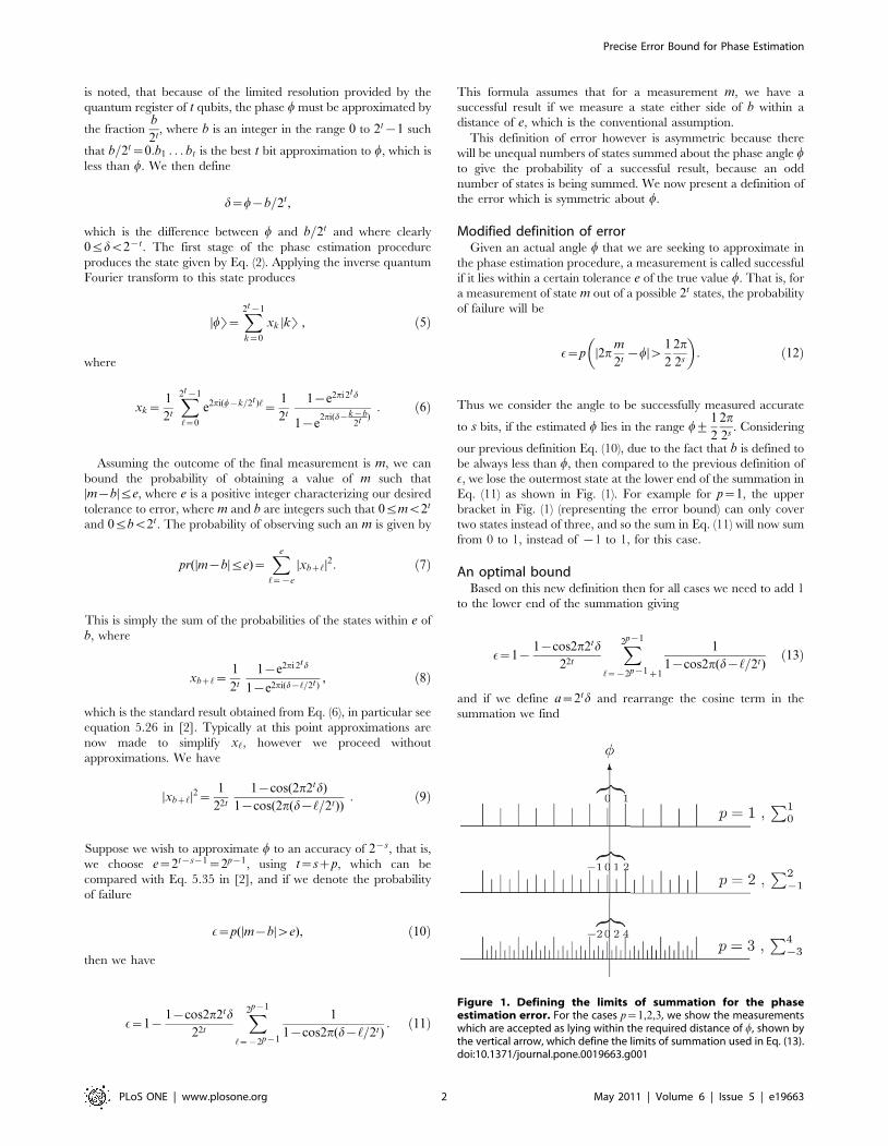
is noted, that because of the limited resolution provided by the
quantum register of t qubits, the phase wmust be approximated by
the fractionb
2t, where b is an integer in the range 0 to 2t1 such
that b=2t~0:b1 . . . bt is the best t bit approximation to w, which is
less than w. We then define
d~wb=2t,
which is the difference between w and b=2t and where clearly
0ƒdv2t. The first stage of the phase estimation procedure
produces the state given by Eq. (2). Applying the inverse quantum
Fourier transform to this state produces
DwT~X
2t1
k~0
xk DkT , ð5Þ
where
xk~1
2t
X
2t1
‘~0
e2pi(wk=2t)‘~
1
2t1e2pi 2
td
1e2pi(dkb
2t): ð6Þ
Assuming the outcome of the final measurement is m, we can
bound the probability of obtaining a value of m such that
DmbDƒe, where e is a positive integer characterizing our desired
tolerance to error, where m and b are integers such that 0ƒmv2t
and 0ƒbv2t. The probability of observing such an m is given by
pr(DmbDƒe)~X
e
‘~e
Dxbz‘D2: ð7Þ
This is simply the sum of the probabilities of the states within e of
b, where
xbz‘~1
2t1e2pi 2
td
1e2pi(d‘=2t), ð8Þ
which is the standard result obtained from Eq. (6), in particular see
equation 5.26 in [2]. Typically at this point approximations are
now made to simplify x‘, however we proceed without
approximations. We have
Dxbz‘D2~
1
22t1cos(2p2td)
1cos(2p(d‘=2t)): ð9Þ
Suppose we wish to approximate w to an accuracy of 2s, that is,
we choose e~2ts1~2p1, using t~szp, which can be
compared with Eq. 5.35 in [2], and if we denote the probability
of failure
E~p(DmbDwe), ð10Þ
then we have
E~11cos2p2td
22t
X
2p1
‘~2p1
1
1cos2p(d‘=2t): ð11Þ
This formula assumes that for a measurement m, we have a
successful result if we measure a state either side of b within a
distance of e, which is the conventional assumption.
This definition of error however is asymmetric because there
will be unequal numbers of states summed about the phase angle wto give the probability of a successful result, because an odd
number of states is being summed. We now present a definition of
the error which is symmetric about w.
Modified definition of errorGiven an actual angle w that we are seeking to approximate in
the phase estimation procedure, a measurement is called successful
if it lies within a certain tolerance e of the true value w. That is, fora measurement of state m out of a possible 2t states, the probability
of failure will be
E~p D2pm
2twDw
1
2
2p
2s
: ð12Þ
Thus we consider the angle to be successfully measured accurate
to s bits, if the estimated w lies in the range w+1
2
2p
2s. Considering
our previous definition Eq. (10), due to the fact that b is defined to
be always less than w, then compared to the previous definition of
E, we lose the outermost state at the lower end of the summation in
Eq. (11) as shown in Fig. (1). For example for p~1, the upper
bracket in Fig. (1) (representing the error bound) can only cover
two states instead of three, and so the sum in Eq. (11) will now sum
from 0 to 1, instead of 1 to 1, for this case.
An optimal boundBased on this new definition then for all cases we need to add 1
to the lower end of the summation giving
E~11cos2p2td
22t
X
2p1
‘~2p1z1
1
1cos2p(d‘=2t)ð13Þ
and if we define a~2td and rearrange the cosine term in the
summation we find
Figure 1. Defining the limits of summation for the phaseestimation error. For the cases p~1,2,3, we show the measurementswhich are accepted as lying within the required distance of w, shown bythe vertical arrow, which define the limits of summation used in Eq. (13).doi:10.1371/journal.pone.0019663.g001
Precise Error Bound for Phase Estimation
PLoS ONE | www.plosone.org 2 May 2011 | Volume 6 | Issue 5 | e19663

E~11cos2pa
22tz1
X
2p1
‘~2p1z1
csc2p
2t(a‘): ð14Þ
Next, we demonstrate that the right hand side of Eq. (14) takes
its maximum value at a~1
2. Since we know 0ƒav1, and since
we expect the maximum value of E~E(a,t,p) to lie about midway
between the two nearest states to generate the largest error, that is
at a~1=2, we will substitute a~1
2zD, where D%
1
2. To
maximize E we need to minimize
cos2p1
2zD
X
2p1
‘~2p1z1
csc2p
2t1
2‘zD
, ð15Þ
as a function of D. Expanding to quadratic order with a Taylor
series, we seek to minimize
1p2D2zO(D4)
c0zc1Dzc2D2zc3D
3zO(D4)
, ð16Þ
where ci are the coefficients of the Taylor expansion of cosecant2
in D. We find by the odd symmetry of the cotangent about ‘~1
2that
c1~2p
2t
X
2p1
‘~2p1z1
cotp
2t(1
2‘) csc2
p
2t(1
2‘)~0, ð17Þ
and so we just need to minimize
c0z(c2c0p2)D2
zO(D3): ð18Þ
Differentiating, we see we have an extremum at D~0, and
therefore E(a,t,p) has a maximum at a~1=2.
Substituting a~1
2we obtain
Eƒ12
22t
X
2p1
‘~2p1z1
1
1cos2p
2t(1
2‘)
: ð19Þ
We note that the summation is symmetrical about ‘~1=2, andsubstituting t~pzs, we obtain for our final result
E(s,p)~11
22(pzs)2
X
2p1
‘~1
1
1cosp(2‘1)
2(pzs)
: ð20Þ
That is, given a desired accuracy of s bits, then if we add p more
bits, we have a probability of success given by 1E, of obtaining a
measurement to at least s bits of accuracy. Thus we have
succeeded in deriving a best possible bound for the failure rate
E~E(s,p).
Special CasesNumerical calculations show that E(t,p) quickly approaches its
asymptotic value as t??, and this limit gives a fairly accurate
upper bound for E, for t greater than about 10 qubits. Using
cosx§1x2
2which is valid for all x, and is accurate for
x~O(1=2t) as t??,
Eƒ14
22t
X
2p1
‘~1
1
1(11
2(p
2t(2‘1))2)
~18
p2
X
2p1
‘~1
1
(2‘1)2
ð21Þ
An exact form for this can be found in terms of the trigamma
function, being a special case of the polygamma function as shown
in Abramowitz and Stegun [6], Eq. 6.4.5:
Eƒ2
p2y’
1z2p
2
ð22Þ
where y’(z)~dy
dzis the trigamma function, y(z)~
C’(z)
C(z)is the
digamma function, and C(z)~
ð?
0
tz1etdt is the standard
gamma function.
Now considering the p?? limit, which also includes the t??
limit because t~pzs, we can find an asymptotic form in the limit
of large p also from [6], Eq. 6.4.12, namely
E~4
p22p, ð23Þ
which shows that the error rate drops off exponentially with p
extra qubits. The formula Eq. (23) can be re-arranged to give
p?~qlog22
ffiffiffi
2p
p2Er ð24Þ
which can be compared with the previous approximate formula
shown in Eq. (1).
We have checked the new error formula through simulations,
by running the phase estimation algorithm on a 2-dimensional
rotation matrix, and undertaking a numerical search for the
rotation angle that maximizes the error E, which has confirmed
Eq. (20) to six decimal places.
Discussion
An exact formula is derived for the probability of error in the
quantum phase estimation procedure, as shown in Eq. (20). That
is, to calculate w accurate to a required s bits with a given
probability of success 1E we add p extra qubits, where p is given
by Eq. (20). If we have a large number of qubits then we can use
Eq. (22) valid at the t?? limit. In the p?? limit the asymptote
is found as a simple exponential form Eq. (23).
The exact formula avoids overestimating the number of qubits
actually required in order to achieve a given reliability for phase
estimation and we have also found this formula to be useful in
confirming the operation of classical simulators of the phase
estimation procedure.
Precise Error Bound for Phase Estimation
PLoS ONE | www.plosone.org 3 May 2011 | Volume 6 | Issue 5 | e19663

Acknowledgments
Discussions with Anthony G. Williams and Sanjeev Naguleswaran during
the early stages of this work are gratefully acknowledged.
Author Contributions
Analyzed the data: MAL LvS JMC AI DA. Contributed reagents/
materials/analysis tools: DA. Wrote the paper: JMC AI. Proofreading:
MAL AI DA.
References
1. Shor PW (1997) Polynomial-time algorithms for prime factorization and discretelogarithms on a quantum computer. SIAM, J Comp 26(5): 1484–1509.
2. Nielsen MA, Chuang IL (2002) Quantum Computation and QuantumInformation. Cambridge UK: Addison-Wesley, first edition.
3. Cleve R, Ekert A (1998) Quantum algorithms revisited. Proc R Soc London A454(1969): 339–354.
4. Imre S, Balazs F (2002) A tight bound for probability of error for quantumcounting based multiuser detection. Proc ISIT 2002: 43.
5. Mosca M (1999) Quantum Computer Algorithms. Ph.D. thesis, University ofOxford.
6. Abramowitz M, Stegun IA (1964) Handbook of Mathematical Functions withFormulas, Graphs, and Mathematical Tables. New York: Dover.
Precise Error Bound for Phase Estimation
PLoS ONE | www.plosone.org 4 May 2011 | Volume 6 | Issue 5 | e19663

Analyzing Three-Player Quantum Games in an EPR Type
Setup
James M. Chappell1,2*, Azhar Iqbal2, Derek Abbott2
1 School of Chemistry and Physics, University of Adelaide, Adelaide, South Australia, Australia, 2 School of Electrical and Electronic Engineering, University of Adelaide,
Adelaide, South Australia, Australia
Abstract
We use the formalism of Clifford Geometric Algebra (GA) to develop an analysis of quantum versions of three-player non-cooperative games. The quantum games we explore are played in an Einstein-Podolsky-Rosen (EPR) type setting. In thissetting, the players’ strategy sets remain identical to the ones in the mixed-strategy version of the classical game that isobtained as a proper subset of the corresponding quantum game. Using GA we investigate the outcome of a realization ofthe game by players sharing GHZ state, W state, and a mixture of GHZ and W states. As a specific example, we study thegame of three-player Prisoners’ Dilemma.
Citation: Chappell JM, Iqbal A, Abbott D (2011) Analyzing Three-Player Quantum Games in an EPR Type Setup. PLoS ONE 6(7): e21623. doi:10.1371/journal.pone.0021623
Editor: Attila Szolnoki, Hungarian Academy of Sciences, Hungary
Received April 13, 2011; Accepted June 3, 2011; Published July 27, 2011
Copyright: 2011 Chappell et al. This is an open-access article distributed under the terms of the Creative Commons Attribution License, which permitsunrestricted use, distribution, and reproduction in any medium, provided the original author and source are credited.
Funding: The authors have no support or funding to report.
Competing Interests: The authors have declared that no competing interests exist.
* E-mail: [email protected]
Introduction
The field of game theory [1,2] has a long history [3], but was
first formalized in 1944 with the work of von Neumann and
Morgenstern [4], aiming to develop rational analysis of situations
that involve strategic interdependence.
Classical game theory has found increasing expression in the
field of physics [3] and its extension to the quantum regime [5] was
proposed by Meyer [6] and Eisert et al [7], though its origins can
be traced to earlier works [8–11]. Early studies in the area of
quantum games focused on the two-player two-strategy non-
cooperative games, with the proposal for a quantum Prisoners’
Dilemma (PD) being well known [7]. A natural further develop-
ment of this work was its extension to multiplayer quantum games
that was explored by Benjamin and Hayden [12]. Du et al. [13,14]
explored the phase transitions in quantum games for the first time
that are central in the present article.
The usual approach in three-player quantum games considers
players sharing a three-qubit quantum state with each player
accessing their respective qubit in order to perform local unitary
transformation. Quantum games have been reported [15] in which
players share Greenberger-Horne-Zeilinger (GHZ) states and theW
states [5], while other works have, for instance, investigated the
effects of noise [16,17] and the benefits of players forming coalitions
[18,19].
A suggested approach [20–23] in constructing quantum games
uses an Einstein-Podolsky-Rosen (EPR) type setting [24–31]. In
this approach, quantum games are setup with an EPR type
apparatus, with the players’ strategies being local actions related to
their qubit, consisting of a linear combination (with real coef-
ficients) of (spin or polarization) measurements performed in two
selected directions.
Note that in a standard arrangement for playing a mixed-
strategy game, players are faced with the identical situation, in that
in each run, a player has to choose one out of two pure strategies.
As the players’ strategy sets remain classical, the EPR type setting
avoids a well known criticism [32] of quantum games. This cri-
ticism refers to quantization procedures in which players are given
access to extended strategy sets, relative to what they are allowed
to have in the classical game. Quantum games constructed with an
EPR type setting have been studied in situations involving two
players [22] and also three players [23]. The applications of three-
player quantum games include describing three-party situations,
involving strategic interaction in quantum communication [33].
In recent works, the formalism of Clifford’s geometric algebra
(GA) [34–38] has been applied to the analysis of two-player
quantum games with significant benefits [39,40], and so is also
adopted here in the analysis of three-player quantum games. The
use of GA is justified on the grounds that the Pauli spin algebra is a
matrix representation of Clifford’s geometric algebra in R3, and
hence we are choosing to work directly with the underlying
Clifford algebra. There are also several other documented benefits
of GA such as:
a) The unification of the dot and cross product into a single
product, has the significant advantage of possessing an
inverse. This results in increased mathematical compactness,
thereby aiding physical intuition and insight [41].
b) The use of the Pauli and Dirac matrices also unnecessarily
introduces the imaginary scalars, in contrast to GA, which
uses exclusively real elements [42]. This fact was also pointed
out by Sommerfield in 1931, who commented that ‘Dirac’s use
of matrices simply rediscovered Clifford algebra’ [43].
c) In the density matrix formalism of quantum mechanics, the
expectation for an operator Q is given by Tr rQð Þ~SyjQjyT, from which we find the isomorphism to GA,
Tr rQð Þ<SrQT0, the subscript zero, indicating to take the
scalar part of the algebraic product rQ, where r and Q are
PLoS ONE | www.plosone.org 1 July 2011 | Volume 6 | Issue 7 | e21623

now constructed from real Clifford elements. This leads to a
uniquely compact expression for the overlap probability
between two states in the N-particle case, given by Eq. (13),
which allows straightforward calculations that normally
require 8|8 complex matrices representing operations on
three qubits.
d) Pauli wave functions are isomorphic to the quaternions, and
hence represent rotations of particle states [44]. This fact
paves the way to describe general unitary transformations on
qubits, in a simplified algebraic form, as rotors. In regard to
Hestenes’ analysis of the Dirac equation using GA, Boudet
[41] notes that, ‘the use of the pure real formalism of
Hestenes brings noticeable simplifications and above all the
entire geometrical clarification of the theory of the electron. ’
e) Recent works [6,39,40] show that GA provides a better
intuitive understanding of Meyer’s quantum penny flip game
[6], using operations in 3-space with real coordinates, permitting
helpful visualizations in determining the quantum player’s
winning strategy. Also, Christian [45,46] has recently used
GA to produce thought provoking investigations into some of
the foundational questions in quantum mechanics.
Our quantum games use an EPR type setting and players have
access to general pure quantum states. We determine constraints
that ensure a faithful embedding of the mixed-strategy version of
the original classical game within the corresponding quantum
game. We find how a Pareto-optimal quantum outcome emerges
in three-player quantum PD game at high entanglement. We also
report phase transitions taking place with increasing entanglement
when players share a mixture of GHZ and W type states in
superposition.
In an earlier paper [23], two of the three authors contributed to
developing an entirely probabilistic framework for the analysis of
three-player quantum games that are also played using an EPR
type setting, whereas the present paper, though using an EPR type
setting, provides an analysis from the perspective of quantum
mechanics, with the mathematical formalism of GA. The previous
work analyzed quantum games from the non-factorizable property
of a joint probability distribution relevant to a physical system that
the players shared in order to implement the game. For the game
of three-player Prisoners’ Dilemma, our probabilistic analysis
showed that non-factorizability of a joint probability distribution
indeed can lead to a new equilibrium in the game. The three-
player quantum Prisoners’ Dilemma, in the present analysis,
however, moves to the next step and explores the phase structure
relating players’ payoffs with shared entanglement and also the
impact of players sharing GHZ and W states and their mixture.
We believe that without using the powerful formalism of GA, a
similar analysis will nearly be impossible to perform using an
entirely probabilistic approach as developed in [22].
EPR setting for playing quantum gamesThe EPR setting [20,22,23] two player quantum games involves
a large number of runs when, in a run, two halves of an EPR pair
originate from the same source and move in the opposite
directions. Player Alice receives one half whereas player Bob
receives the other half. To keep the non-cooperative feature of the
game, it is assumed that players Alice and Bob are located at some
distance from each other and are not unable to communicate
between themselves. The players, however, can communicate
about their actions, which they perform on their received halves,
to a referee who organizes the game and ensures that the rules of the
game are followed. The referee makes available two directions to
each player. In a run, each player has to choose one of two
available directions. The referee rotates Stern-Gerlach type
detectors [5] along the two chosen directions and performs
quantum measurement. The outcome of the quantum measure-
ment, on Alice’s side, and on Bob’s side of the Stern-Gerlach
detectors, is either z1 or 1. Runs are repeated as the players
receive a large number of halves in pairs, when each pair comes
from the same source and the measurement outcomes are
recorded for all runs. A player’s strategy, defined over a large
number of runs, is a linear combination (with normalized and real
coefficients) of the two directions along which the measurement is
performed. The referee makes public the payoff relations at the
start of the game and announces rewards to the players after the
completion of runs. The payoff relations are constructed in view of
a) the matrix of the game, b) the list of players’ choices of direc-
tions over a large number of runs, and c) the list of measurement
outcomes that the referee prepares using his/her Stern-Gerlach
apparatus.
For a three-player quantum game, this setting is extended to
consider three players Alice, Bob and Chris who are located at the
three arms of an EPR system [5]. In the following they will be
denoted by A, B and C, respectively. As it is the case with two-
player EPR setting, in a run of the experiment, each player
chooses one out of two directions.
We have used the EPR setting in view of the well known Enk
and Pike’s criticism [32] of quantum games that are played using
Eisert et al’s setting [7]. Essentially this criticism attempts to equate
a quantum game to a classical game in which the players are given
access to an extended set of classical strategies. The present paper
uses an EPR setting in which each player has two classical
strategies consisting of the two choices he/she can make between
two directions along which a quantum measurement can be
performed. That is, the player’s pure strategy, in a run, consists of
choosing one direction out of the two. As the sets of strategies
remain exactly identical in both the classical and the quantum
forms of the game, it is difficult to construct an Enk and Pike type
argument for a quantum game that is played with an EPR setting.
As Fig. 1 shows, we represent Alice’s two directions as k11,k12.
Similarly, Bob’s directions are k21,k22 and Chris’ are k31,k
32. The
players measurement directions form a triplet out of eight possible
cases k11,k21,k
31
, k11,k22,k
31
, k12,k21,k
31
, k12,k22,k
31
, k11,k21,k
32
,
k11,k22,k
32
, k12,k21,k
32
, k12,k22,k
32
and measurement is performed
along the chosen directional triplet. The measurement outcome
for each player along their chosen direction is z1 or 1.
Over a large number of runs the players sequentially receive
three-particle systems emitted from a source and a record is
maintained of the players’ choices of directions over all runs. One
of the eight possible outcomes z1,z1,z1ð Þ, z1,1,z1ð Þ,1,z1,z1ð Þ, 1,1,z1ð Þ, z1,z1,1ð Þ, z1,1,1ð Þ,1,z1,1ð Þ, 1,1,1ð Þ emerges out of the measurement
in an individual run, with the first entry for Alice’s outcome, the
second entry for Bob’s outcome and the third entry for Chris’
outcome.
In the following we express the players’ payoff relations in terms
of the outcomes of these measurements. These payoffs depend on
the triplets of the players’ strategic choices made over a large
number of runs and on the dichotomic outcomes of the mea-
surements performed along those directions.
Players’ sharing a symmetric initial stateWe consider the situation in which an initial quantum state of
three qubits is shared among three players. To obtain a fair game,
we assume this state is symmetric with regard to the interchange of
the three players. The GHZ state is a natural candidate given by
Three-Player Quantum Games
PLoS ONE | www.plosone.org 2 July 2011 | Volume 6 | Issue 7 | e21623

jGHZT~cosc
2j000Tzsin
c
2j111T, ð1Þ
where we have an entanglement angle c[<, which has been shown
[5] to be capable of producing the maximally entangled three
qubit state. Alternatively we could start with the W entangled state
jWT~1ffiffiffi
3p j100Tzj010Tzj001Tð Þ: ð2Þ
The other symmetric state would be an inverted W state
j WWT~1ffiffiffi
3p j110Tzj011Tzj101Tð Þ: ð3Þ
After the measurement along three directions selected by the
players, each player is rewarded according to a payoff matrix GP ,for each player P[fA,B,Cg. Thus the expected payoffs for a
player is given by
PP k1,k2,k3
~
X
1
i,j,k~0
GPijkPijk, ð4Þ
where Pijk is the probability the state jiTjjTjkT is obtained after
measurement, with i,j,k[f0,1g, along the three directions k1,k2,k3chosen by Alice, Bob and Chris respectively. In the EPR setting,
k1 can be either of Alice’s two directions i.e. k11 or k12 and similarly
for Bob and Chris.
Clifford’s geometric algebraThe formalism of GA [34–38] has been shown to provide an
equivalent description to the conventional tensor product
formalism of quantum mechanics.
To set up the GA framework for representing quantum states,
we begin by defining s1,s2,s3 as a right-handed set of
orthonormal basis vectors, with
si:sj~dij , ð5Þ
where dij is Kronecker delta. Multiplication between algebraic
elements is defined to be the geometric product, which for two
vectors u and v is given by
uv~u:vzu ^ v, ð6Þ
where u:v is the conventional symmetric dot product and u ^ v is
the anti-symmetric outer product related to the Gibb’s cross
product by u|v~iu ^ v, where i~s1s2s3. For distinct basis
vectors we find
sisj~si:sjzsi ^ sj~si ^ sj~sj ^ si~sjsi: ð7Þ
This can be summarized by
sisj~dijzieijksk, ð8Þ
where eijk is the Levi-Civita symbol. We can therefore see that i
squares to minus one, that is i2~s1s2s3s1s2s3~s1s2s1s2~1
and commutes with all other elements and so has identical
properties to the unit imaginary i. Thus we have an isomorphism
between the basis vectors s1,s2,s3 and the Pauli matrices through
the use of the geometric product.
In order to express quantum states in GA we use the one-to-one
mapping [36,38] defined as follows
jyT~aj0Tzbj1T~a0zia3
a2zia1
" #
<y
~a0za1is1za2is2za3is3,
ð9Þ
where ai are real scalars.
For a single particle we then have the basis vectors
j0T<1, j1T<is2 ð10Þ
and so for three particles we can use as a basis
j0Tj0Tj0T<1 ð11aÞ
j0Tj0Tj1T<is32 ð11bÞ
j0Tj1Tj0T<is22 ð11cÞ
j0Tj1Tj1T<is22is32, ð11dÞ
j1Tj0Tj0T<is12 ð11eÞ
j1Tj0Tj1T<is12is32 ð11fÞ
Figure 1. The EPR setup for three-player quantum game. Athree-qubit entangled quantum state is distributed to the three players,who each choose between two possible measurement directions.doi:10.1371/journal.pone.0021623.g001
Three-Player Quantum Games
PLoS ONE | www.plosone.org 3 July 2011 | Volume 6 | Issue 7 | e21623

j1Tj1Tj0T<is12is22 ð11gÞ
j1Tj1Tj1T<is12is22is
32, ð11hÞ
where to reduce the number of superscripts representing particle
number we write i1s12 as is12. General unitary operations are
equivalent to rotors in GA [36], represented as
R h1,h2,h3ð Þ~eh3is3=2eh1is2=2eh2is3=2, ð12Þ
which is in Euler angle form and can completely explore the available
space of a single qubit. Using the definition of unitary operations
given by Eq. (12) we define A~R a1,a2,a3ð Þ, B~R b1,b2,b3ð Þ,C~R x1,x2,x3ð Þ for general unitary transformations acting locally
on each of the three players qubit in order to generalize the starting
state, that is the GHZ or W states, as far as possible.
We define a separable state w~KLM, where K , L and M are
single particle rotors, which allow the players’ measurement
directions to be specified on the first, second and third qubit
respectively. The state to be measured is now projected onto this
separable state w. The overlap probability between two states yand w in the N-particle case is given in Ref. [36] as
P y,wð Þ~2N2 SyEywEwT0SyJywJwT0
h i
, ð13Þ
where the angle brackets ST0 mean to retain only the scalar part of
the expression and E and J are defined for 3 particles in Ref. [36] as
E~ PN
i~2
1
21is13is
i3
~1
41is13is
23is13is
33is23is
33
ð14aÞ
J~Eis13~1
4is13zis23zis33is13is
23is
33
: ð14bÞ
The operator acts the same as complex conjugation: flipping
the sign of i and inverting the order of the terms.
Results
We now, firstly, calculate the observables from Eq. (11) for the
GHZ state in GA, which from Eq. (11) gives
y~ABC cosc
2sin
c
2is12is
22is
32
, ð15Þ
where A, B, and C represent the referee’s local unitary actions,
written as rotors A, B, and C in GA, on the respective player’s
qubits, in order to generalize the starting state. Referring to Eq.
(13), we firstly calculate
yJy~
1
4ABC cos
c
2sin
c
2is12is
22is
32
is13zis23zis33is13is23is
33
| cosc
2zsin
c
2is12is
22is
32
CBA
~1
4ABC cos csin cis12is
22is
32
is13zis23zis33is13is23is
33
CBA
~1
4cos c R3zS3zT3R3S3T3ð Þ
zsin c R1S2T2zR2S1T2zR2S2T1R1S1T1ð Þ
ð16Þ
where Rk~iAskA,Sk~iBskB
,Tk~iCskC.
We also calculate
yEy~
1
4ABC cos
c
2sin
c
2is12is
22is
32
1is13is23is13is
33is23is
33
| cosc
2zsin
c
2is12is
22is
32
CBA
~1
4ABC 1is13is
23is13is
33is23is
33
CBA
~1
41R3S3R3T3S3T3ð Þ:
ð17Þ
For measurement defined with K~eiks1
2=2, L~e
iks22=2
and
M~eiks3
2=2
allowing a rotation of the detectors by an angle k,
where we have written k1s12 as ks12, we find
wJw~
1
4is13e
iks12zis23e
iks22zis33e
iks32is13is
23is
33e
iks12e
iks22e
iks32
ð18aÞ
wEw~
1
41is13is
23e
iks12e
iks22is13is
33e
iks12e
iks32is23is
33e
iks22e
iks32
:ð18bÞ
From Eq. (13) we find
2SyEywEwT~1
81R3S3R3T3S3T3ð Þ
|(1is13is23e
iks12e
iks22is13is
33e
iks12e
iks32is23is
33e
iks22e
iks32 )
~1
81z()lzmX (k1)Y (k2)z()lznX (k1)Z(k3)
z()mznY (k2)Z(k3)
~1
81z()lzmXiYjz
()lznXiZkz()mznYjZk
,
ð19Þ
where l,m,n[f0,1g refers to measuring a j0T or j1T state,
respectively, and using the standard results listed in the Appendix
S1, we have
Xi~X k1i
~cos a1 cosk1i zcos a3 sin a1 sin k
1i , ð20aÞ
Yj~Y k2j
~cosb1 cos k2j zcos b3 sinb1 sin k
2j , ð20bÞ
Zk~Z k3k
~cos x1 cosk3kzcos x3 sin x1 sink
3k, ð20cÞ
with i,j,k[f1,2g, representing the two measurement directions
Three-Player Quantum Games
PLoS ONE | www.plosone.org 4 July 2011 | Volume 6 | Issue 7 | e21623

available to each player. Also from Eq. (13) we have
2SyJywJwT~1
8S(cos c(R3zS3zT3R3S3T3)
z sin c(R1S2T2zR2S1T2zR2S2T1R1S1T1))
|(is13eiks1
2zis23eiks2
2zis33eiks3
2is13is23is
33e
iks12e
iks22e
iks32 )T0
~1
8(cos c(()lXiz()mYjz()nZkz()lmnXiYjZk)
z()lmn sin c(FiVjWkzUiGjWkzUiVjHkFiGjHk))
~1
8½cos cf()lXiz()mYjz()nZkz()lmnXiYjZkg
z()lmn sin cHijk,
ð21Þ
where
Fi~F k1
~sink1i cos a1 cos a2 cos a3sin a2 sin a3ð Þ
zsin a1 cos a2 cos k1i ,
ð22aÞ
Gj~G k2
~sink2j cos b1 cos b2 cos b3sinb2 sinb3ð Þ
zsin b1 cosb2 cos k2j ,
ð22bÞ
Hk~H k3
~sink3k cos x1 cos x2 cos x3sin x2 sin x3ð Þ
zsin x1 cos x2 cos k3k
ð22cÞ
and
Ui~U k1
~sin k1i cos a2 sin a3zsin a2 cos a3 cos a1ð Þ
sin a1 sin a2 cos k1i ,
ð23aÞ
Vj~V k2
~sink2j cos b2 sin b3zsin b2 cos b3 cos b1ð Þ
sinb1 sin b2 cos k2j ,
ð23bÞ
Wk~W k3
~sink3k cos x2 sin x3zsin x2 cos x3 cos x1ð Þ
sin x1 sin x2 cosk3k
ð23cÞ
and
Hijk~FiVjWkzUiGjWkzUiVjHkFiGjHk: ð24Þ
So we find from Eq. (13) the probability to observe a particular
state after measurement as
Plmn~1
8½1zcos cf ð ÞlXiz ð ÞmYjz ð ÞnZkg
z ð ÞlmXiYjz ð ÞlnXiZkz ð ÞmnYjZk
z ð Þlmnfcos cXiYjZkzsin cHijkg:
ð25Þ
For instance, at c~0 we obtain
Plmn~1
81z ð ÞlXi
1z ð ÞmYj
1z ð ÞnZkð Þ, ð26Þ
which shows a product state, as expected. Alternatively with
general entanglement, but no operation on the third qubit, that is
xi~0, we have
Plm~1
8½1zcos cf ð ÞlXiz ð ÞmYjz1z ð Þlmn
XiYjg
z ð ÞlmXiYjz ð ÞlXiz ð ÞmYj :
~1
8½ 1zcos cð Þ 1z ð ÞlXi
1z ð ÞmYj
,
ð27Þ
which shows that for the GHZ type entanglement each pair of
qubits is mutually unentangled.
Obtaining the payoff relationsWe extend the approach of Ichikawa and Tsutsui [47] to three
qubits and represent the permutation of signs introduced by the
measurement process. For Alice we define
a000~1
8
X
ijk
GAijk, a100~
1
8
X
ijk
ð ÞiGAijk, ð28aÞ
a010~1
8
X
ijk
ð ÞjGAijk, a001~
1
8
X
ijk
ð ÞkGAijk, ð28bÞ
a110~1
8
X
ijk
ð ÞizjGA
ijk, a011~1
8
X
ijk
ð ÞjzkGA
ijk, ð28cÞ
a101~1
8
X
ijk
ð ÞizkGA
ijk, a111~1
8
X
ijk
ð ÞizjzkGA
ijk: ð28dÞ
Using Eq. (4), we then can find the payoff for each player
PA k1i ,k2j ,k
3k
~a000zcos cfa100Xiza010Yjza001Zkg
za110XiYjza101XiZkza011YjZk
za111fcos cXiYjZkzsin cHijkg,
ð29aÞ
PB k1i ,k2j ,k
3k
~b000zcos cfb100Xizb010Yjzb001Zkg
zb110XiYjzb101XiZkzb011YjZk
zb111fcos cXiYjZkzsin cHijkg,
ð29bÞ
PC k1i ,k2j ,k
3k
~c000zcos cfc100Xizc010Yjzc001Zkg
zc110XiYjzc101XiZkzc011YjZk
zc111fcos cXiYjZkzsin cHijkg,
ð29cÞ
where, as Eqs. (20) show, the three measurement directions
Three-Player Quantum Games
PLoS ONE | www.plosone.org 5 July 2011 | Volume 6 | Issue 7 | e21623
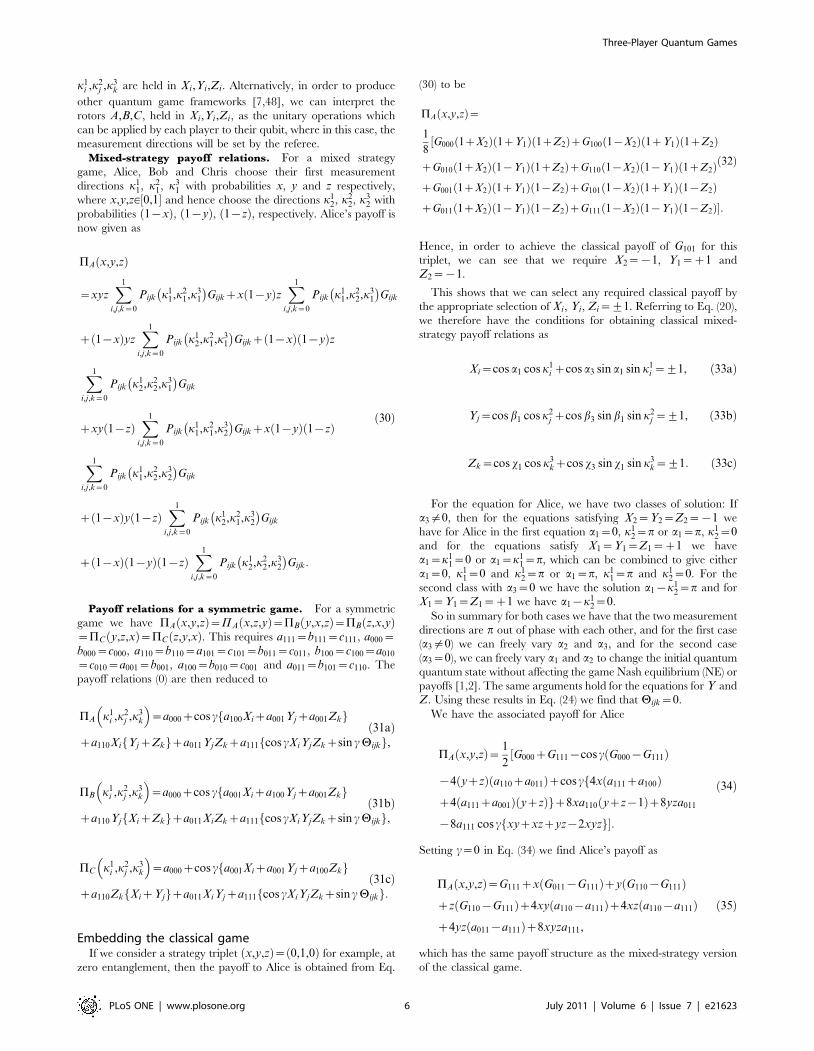
k1i ,k2j ,k
3k are held in Xi,Yi,Zi. Alternatively, in order to produce
other quantum game frameworks [7,48], we can interpret the
rotors A,B,C, held in Xi,Yi,Zi, as the unitary operations which
can be applied by each player to their qubit, where in this case, the
measurement directions will be set by the referee.
Mixed-strategy payoff relations. For a mixed strategy
game, Alice, Bob and Chris choose their first measurement
directions k11, k21, k
31 with probabilities x, y and z respectively,
where x,y,z[ 0,1½ and hence choose the directions k12, k22, k
32 with
probabilities 1xð Þ, 1yð Þ, 1zð Þ, respectively. Alice’s payoff isnow given as
PA x,y,zð Þ
~xyzX
1
i,j,k~0
Pijk k11,k21,k
31
Gijkzx 1yð ÞzX
1
i,j,k~0
Pijk k11,k22,k
31
Gijk
z 1xð ÞyzX
1
i,j,k~0
Pijk k12,k21,k
31
Gijkz 1xð Þ 1yð Þz
X
1
i,j,k~0
Pijk k12,k22,k
31
Gijk
zxy 1zð ÞX
1
i,j,k~0
Pijk k11,k21,k
32
Gijkzx 1yð Þ 1zð Þ
X
1
i,j,k~0
Pijk k11,k22,k
32
Gijk
z 1xð Þy 1zð ÞX
1
i,j,k~0
Pijk k12,k21,k
32
Gijk
z 1xð Þ 1yð Þ 1zð ÞX
1
i,j,k~0
Pijk k12,k22,k
32
Gijk:
ð30Þ
Payoff relations for a symmetric game. For a symmetric
game we have PA x,y,zð Þ~PA x,z,yð Þ~PB y,x,zð Þ~PB z,x,yð Þ~PC y,z,xð Þ~PC z,y,xð Þ. This requires a111~b111~c111, a000~
b000~c000, a110~b110~a101~c101~b011~c011, b100~c100~a010~c010~a001~b001, a100~b010~c001 and a011~b101~c110. The
payoff relations (0) are then reduced to
PA k1i ,k2j ,k
3k
~a000zcos cfa100Xiza001Yjza001Zkg
za110XifYjzZkgza011YjZkza111fcos cXiYjZkzsin cHijkg,ð31aÞ
PB k1i ,k2j ,k
3k
~a000zcos cfa001Xiza100Yjza001Zkg
za110YjfXizZkgza011XiZkza111fcos cXiYjZkzsin cHijkg,ð31bÞ
PC k1i ,k2j ,k
3k
~a000zcos cfa001Xiza001Yjza100Zkg
za110ZkfXizYjgza011XiYjza111fcos cXiYjZkzsin cHijkg:ð31cÞ
Embedding the classical gameIf we consider a strategy triplet x,y,zð Þ~ 0,1,0ð Þ for example, at
zero entanglement, then the payoff to Alice is obtained from Eq.
(30) to be
PA x,y,zð Þ~1
8½G000 1zX2ð Þ 1zY1ð Þ 1zZ2ð ÞzG100 1X2ð Þ 1zY1ð Þ 1zZ2ð Þ
zG010 1zX2ð Þ 1Y1ð Þ 1zZ2ð ÞzG110 1X2ð Þ 1Y1ð Þ 1zZ2ð ÞzG001 1zX2ð Þ 1zY1ð Þ 1Z2ð ÞzG101 1X2ð Þ 1zY1ð Þ 1Z2ð ÞzG011 1zX2ð Þ 1Y1ð Þ 1Z2ð ÞzG111 1X2ð Þ 1Y1ð Þ 1Z2ð Þ:
ð32Þ
Hence, in order to achieve the classical payoff of G101 for this
triplet, we can see that we require X2~1, Y1~z1 and
Z2~1.
This shows that we can select any required classical payoff by
the appropriate selection of Xi, Yi, Zi~+1. Referring to Eq. (20),
we therefore have the conditions for obtaining classical mixed-
strategy payoff relations as
Xi~cos a1 cosk1i zcos a3 sin a1 sin k
1i ~+1, ð33aÞ
Yj~cos b1 cosk2j zcos b3 sinb1 sink
2j ~+1, ð33bÞ
Zk~cos x1 cos k3kzcos x3 sin x1 sink
3k~+1: ð33cÞ
For the equation for Alice, we have two classes of solution: If
a3=0, then for the equations satisfying X2~Y2~Z2~1 we
have for Alice in the first equation a1~0, k12~p or a1~p, k12~0
and for the equations satisfy X1~Y1~Z1~z1 we have
a1~k11~0 or a1~k11~p, which can be combined to give either
a1~0, k11~0 and k12~p or a1~p, k11~p and k12~0. For the
second class with a3~0 we have the solution a1k12~p and for
X1~Y1~Z1~z1 we have a1k12~0.
So in summary for both cases we have that the two measurement
directions are p out of phase with each other, and for the first case
(a3=0) we can freely vary a2 and a3, and for the second case
(a3~0), we can freely vary a1 and a2 to change the initial quantumquantum state without affecting the game Nash equilibrium (NE) or
payoffs [1,2]. The same arguments hold for the equations forY and
Z. Using these results in Eq. (24) we find that Hijk~0.
We have the associated payoff for Alice
PA x,y,zð Þ~ 1
2½G000zG111cos c G000G111ð Þ
4 yzzð Þ a110za011ð Þzcos cf4x a111za100ð Þz4 a111za001ð Þ yzzð Þgz8xa110 yzz1ð Þz8yza011
8a111 cos cfxyzxzzyz2xyzg:
ð34Þ
Setting c~0 in Eq. (34) we find Alice’s payoff as
PA x,y,zð Þ~G111zx G011G111ð Þzy G110G111ð Þzz G110G111ð Þz4xy a110a111ð Þz4xz a110a111ð Þz4yz a011a111ð Þz8xyza111,
ð35Þ
which has the same payoff structure as the mixed-strategy version
of the classical game.
Three-Player Quantum Games
PLoS ONE | www.plosone.org 6 July 2011 | Volume 6 | Issue 7 | e21623

Now, we can also write the equations governing the NE as
PA x,y,zð ÞPA x,y,zð Þ~ xxð Þ½a110 2y1ð Þza101 2z1ð Þzcos cfa100za111 2y1ð Þ 2z1ð Þg§0
PB x,y,zð ÞPB x,y,zð Þ~ yyð Þ½b110 2x1ð Þzb011 2z1ð Þzcos cfb010zb111 2x1ð Þ 2z1ð Þg§0
PC x,y,zð ÞPC x,y,zð Þ~ zzð Þ½c101 2x1ð Þzc011 2y1ð Þzcos cfc001zc111 2x1ð Þ 2y1ð Þg§0,
ð36Þ
where the strategy triple x,y,zð Þ is a NE. Using the conditions
defined earlier for a symmetric game, we can reduce our equations
governing the NE for the three players to
xxð Þ½2a110 yzz1ð Þzcos cfa100za111 2y1ð Þ 2z1ð Þg§0,
ð37aÞ
yyð Þ½2a110 xzz1ð Þzcos cfa100za111 2x1ð Þ 2z1ð Þg§0,
ð37bÞ
zzð Þ½2a110 xzy1ð Þzcos cfa100za111 2x1ð Þ 2y1ð Þg§0
ð37cÞ
We can see that the new quantum behavior is governed solely by
the payoff matrix through a100, a110 and a111 and by the entang-
lement angle c, and not by other properties of the quantum state.
For completeness, we have Bob’s payoff, in the symmetric case, as
PB x,y,zð Þ~ 1
2½G000zG111cos c G000G111ð Þ
4 xzzð Þ a110za011ð Þzcos c4y a111za100ð Þz4 xzzð Þ a111za001ð Þz8ya110 xzz1ð Þz8xza011
8a111 cos cfxyzxzzyz2xyzg:
ð38Þ
The mixed NE for all players is
x~y~z~a110zcos ca111+
ffiffiffiffiffiffiffiffiffiffiffiffiffiffiffiffiffiffiffiffiffiffiffiffiffiffiffiffiffiffiffiffiffiffiffiffiffiffi
a2110cos ca100a111
q
2 cos ca111: ð39Þ
Maximally entangled case. For c~p=2 at maximum
entanglement for both NE of x,y,zð Þ~ 0,0,0ð Þ and x,y,zð Þ~ 1,1,1ð Þ we have the payoff
PA x,y,zð Þ~PB x,y,zð Þ~PC x,y,zð Þ~ 1
2G000zG111ð Þð40Þ
which gives the average of the two corners of the payoff matrix,
which is as expected.
Prisoners’ Dilemma. An example of a three-player PD
game is shown in Table 1. For this game, from Eq. (28), we have
a000~32=8,a001~14=8, a010~14=8,a011~0,a100~8=8,a101~2=8,a110~2=8,a111~0, with the NE from Eqs. (37) given by
xxð Þ½ yzz1ð Þ2 cos c§0, ð41aÞ
yyð Þ½ xzz1ð Þ2 cos c§0, ð41bÞ
zzð Þ½ xzy1ð Þ2 cos c§0: ð41cÞ
We have the classical NE of x,y,zð Þ~ 0,0,0ð Þ for cos c~1,
but we have a phase transition, as the entanglement increases, at
cos c~1
2where we find the new NE x,y,zð Þ~ 1,0,0ð Þ,
x,y,zð Þ~ 0,1,0ð Þ and x,y,zð Þ~ 0,0,1ð Þ. The payoff for Alice
from Eq. (34) is given by
PA x,y,zð Þ~ 1
2½7z2xz yzzð Þ 12xð Þ
cos cf5z4x7 yzzð Þg:ð42Þ
For the classical region we have PA 0,0,0ð Þ~PB 0,0,0ð Þ~PC 0,0,0ð Þ~ 7
2
5
2cos c, which is graphed in Fig. 2 along with
other parts of the phase diagram. It should be noted that cos c cango negative, which will produce a mirror image about the vertical
axis of the current graph. That is for cos c decreasing from 1
2to
1, we have a NE of x,y,zð Þ~ 1,1,1ð Þ, falling from 2:25 down
to 1. We will also have the NE of x,y,zð Þ~ 1,1,0ð Þ and
x,y,zð Þ~ 0,1,1ð Þ for 1
2cos cv0.
This graph also illustrates the value of coalitions, because if Bob
and Chris both agree to implement the same strategy, then the
only NE available for 0vcos cv1
2for example, is x,y,zð Þ~
1,0,0ð Þ. However, for a NE in the region of cos c just less than one
half, both Bob and Chris receive a significantly greater payoff, of
around 4:5 units, as opposed to 2:5 for Alice, so the coalition will
receive nearly twice the payoff.
Table 1. An example of three-player Prisoners’ Dilemma.
State j000T j001T j010T j100T j011T j101T j110T j111TPayoff (6,6,6) (3,3,9) (3,9,3) (9,3,3) (0,5,5) (5,0,5) (5,5,0) (1,1,1)
The payoff for each player (one,two,three), for each measurement outcome.doi:10.1371/journal.pone.0021623.t001
Three-Player Quantum Games
PLoS ONE | www.plosone.org 7 July 2011 | Volume 6 | Issue 7 | e21623
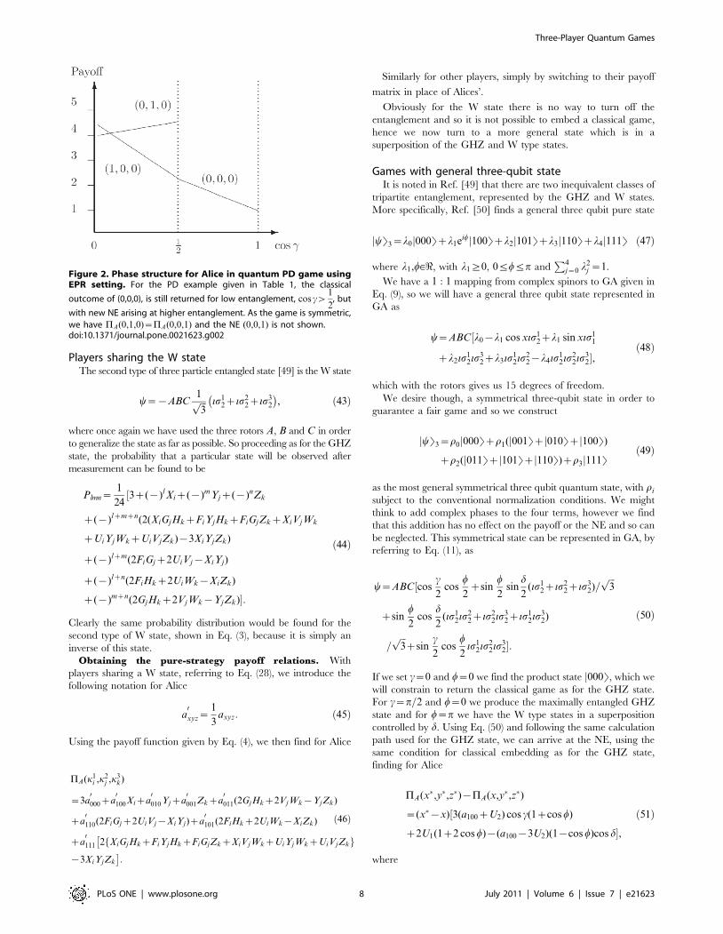
Players sharing the W stateThe second type of three particle entangled state [49] is the W state
y~ABC1ffiffiffi
3p is12zis22zis32
, ð43Þ
where once again we have used the three rotors A, B and C in order
to generalize the state as far as possible. So proceeding as for the GHZ
state, the probability that a particular state will be observed after
measurement can be found to be
Plmn~1
24½3z()lXiz()mYjz()nZk
z()lzmzn(2(XiGjHkzFiYjHkzFiGjZkzXiVjWk
zUiYjWkzUiVjZk)3XiYjZk)
z()lzm(2FiGjz2UiVjXiYj)
z()lzn(2FiHkz2UiWkXiZk)
z()mzn(2GjHkz2VjWkYjZk):
ð44Þ
Clearly the same probability distribution would be found for the
second type of W state, shown in Eq. (3), because it is simply an
inverse of this state.
Obtaining the pure-strategy payoff relations. With
players sharing a W state, referring to Eq. (28), we introduce the
following notation for Alice
a0xyz~
1
3axyz: ð45Þ
Using the payoff function given by Eq. (4), we then find for Alice
PA(k1i ,k
2j ,k
3k)
~3a0000za
0100Xiza
0010Yjza
0001Zkza
0011(2GjHkz2VjWkYjZk)
za0110(2FiGjz2UiVjXiYj)za
0101(2FiHkz2UiWkXiZk)
za0111 2fXiGjHkzFiYjHkzFiGjZkzXiVjWkzUiYjWkzUiVjZkg
3XiYjZk
:
ð46Þ
Similarly for other players, simply by switching to their payoff
matrix in place of Alices’.
Obviously for the W state there is no way to turn off the
entanglement and so it is not possible to embed a classical game,
hence we now turn to a more general state which is in a
superposition of the GHZ and W type states.
Games with general three-qubit stateIt is noted in Ref. [49] that there are two inequivalent classes of
tripartite entanglement, represented by the GHZ and W states.
More specifically, Ref. [50] finds a general three qubit pure state
jyT3~l0j000Tzl1eiwj100Tzl2j101Tzl3j110Tzl4j111T ð47Þ
where l1,w[<, with l1§0, 0ƒwƒp andP4
j~0 l2j ~1.
We have a 1 : 1 mapping from complex spinors to GA given in
Eq. (9), so we will have a general three qubit state represented in
GA as
y~ABC½l0l1 cos xis12zl1 sinxis
11
zl2is12is
32zl3is
12is
22l4is
12is
22is
32,
ð48Þ
which with the rotors gives us 15 degrees of freedom.
We desire though, a symmetrical three-qubit state in order to
guarantee a fair game and so we construct
jyT3~r0j000Tzr1(j001Tzj010Tzj100T)zr2(j011Tzj101Tzj110T)zr3j111T
ð49Þ
as the most general symmetrical three qubit quantum state, with risubject to the conventional normalization conditions. We might
think to add complex phases to the four terms, however we find
that this addition has no effect on the payoff or the NE and so can
be neglected. This symmetrical state can be represented in GA, by
referring to Eq. (11), as
y~ABC½cos c
2cos
w
2zsin
w
2sin
d
2(is12zis22zis32)=
ffiffiffi
3p
zsinw
2cos
d
2(is12is
22zis22is
32zis12is
32)
=ffiffiffi
3p
zsinc
2cos
w
2is12is
22is
32:
ð50Þ
If we set c~0 and w~0 we find the product state j000T, which we
will constrain to return the classical game as for the GHZ state.
For c~p=2 and w~0 we produce the maximally entangled GHZ
state and for w~p we have the W type states in a superposition
controlled by d. Using Eq. (50) and following the same calculation
path used for the GHZ state, we can arrive at the NE, using the
same condition for classical embedding as for the GHZ state,
finding for Alice
PA(x,y,z)PA(x,y
,z)
~(xx)½3(a100zU2) cos c(1zcos w)
z2U1(1z2 cos w)(a1003U2)(1cos w)cos d,ð51Þ
where
Figure 2. Phase structure for Alice in quantum PD game usingEPR setting. For the PD example given in Table 1, the classical
outcome of (0,0,0), is still returned for low entanglement, cos cw1
2, but
with new NE arising at higher entanglement. As the game is symmetric,
we have PA(0,1,0)~PA(0,0,1) and the NE (0,0,1) is not shown.doi:10.1371/journal.pone.0021623.g002
Three-Player Quantum Games
PLoS ONE | www.plosone.org 8 July 2011 | Volume 6 | Issue 7 | e21623

U1~a110 2y1ð Þza101 2z1ð Þ~2a110 yzz1ð Þ ð52aÞ
U2~a111 12yð Þ 12zð Þ: ð52bÞ
We can see the effect of the W type states in the cos d term and so
it illustrates how both types of W states contribute. The reason
they can both appear is because by demanding the classical
embedding we have severely restricted the available unitary
transformations available to transform the starting state.
The payoff relations. The payoff function for Alice given by
PA~a0001
2V1zV3ð Þ cos c 1zcos wð Þz 1
3V2 1z2 cos wð Þ
z1
6V13V3ð Þ 1cos wð Þ cos d,
ð53Þ
where
V1~a100 12xð Þza010 12yð Þza001 12zð Þ ð54aÞ
V2~a110(12x)(12y)
za101(12x)(12z)za011(12y)(12z)ð54bÞ
V3~a111 12xð Þ 12yð Þ 12zð Þ: ð54cÞ
The payoff for Bob and Chris found by simply replacing aijk with
bijk and cijk from their respective payoff matrices. When
comparing with the payoff formula above with the classical
result at x,y,zð Þ~ 0,0,0ð Þ, it is helpful to note that a000za001za010za011za100za101za110za111~G000 and generally a000
z 1ð Þna001z 1ð Þma010z 1ð Þmzna011z 1ð Þla100z
1ð Þlzna101z 1ð Þlzm
a110z 1ð Þlzmzna111~Glmn:
Uniform superposition state. If we select a uniform
superposition state, with r0~r1~r2~r3~1
2, that is,
substituting c~p
2, w~
2p
3and d~
p
2, giving a product state
H63j000T, with H being the Hadamard operator, then we find
that PA x,y,zð ÞPA x,y,zð Þ~0 for Alice, and similarly for
the other players. That is the payoff will be independent of the
player choices and Eq. (53) gives PA~PB~PC~a000. Where
a000 represents the average of all the entries in the payoff matrix,
as expected for a uniform superposition state.
Prisoners’ Dilemma. For the PD game from the previous
section with the GHZ state, we found a100~8=8,a110~2=8,a111~0, so U2~0, with the NE from Eq. (79) for the
three players given by
(xx)½(1yz)(1z2 cos w)
3 cos c(1zcos w)z(1cos w) cos d§0,ð55aÞ
(yy)½(1xz)(1z2 cosw)
3 cos c(1zcos w)z(1cos w) cos d§0,ð55bÞ
(zz)½(1xy)(1z2 cosw)
3 cos c(1zcos w)z(1cos w) cos d§0,ð55cÞ
with the payoff for Alice given by
PA~41
6(12x)(1yz)(1z2 cos w)
1
4(5z4x7y7z)½cos c(1zcosw)
1
3(1cos w) cos d:
ð56Þ
We can see with w~0 we recover the NE for the GHZ state, in
Eq. (37).
Shifting of the NE compared to the GHZ state. We have
the classical NE of x,y,zð Þ~ 0,0,0ð Þ for cos c~1 and cos w~1,
but we can see, that once again, we have a phase transition, as the
entanglement increases, to a new NE of x,y,zð Þ~ 1,0,0ð Þ,x,y,zð Þ~ 0,1,0ð Þ and x,y,zð Þ~ 0,0,1ð Þ.The phase transition will be at cos c~
1
32cos dð Þz
2 cos d1
3 1zcos wð Þ . We notice that as we increase the weighting towards
the W state, by increasing w, that it becomes easier to make the
phase transition in comparison to the pure GHZ state, that is, we
improve access to the phase transition as we introduce the weight
of the j011Tzj101Tzj110T state. In fact, even at cos c~1, we
can achieve the NE of x,y,zð Þ~ 1,1,1ð Þ, with w~p, giving a
payoff of 31
3units.
Maximizing the payoff. Looking at the payoff function for
Alice in Eq. (56), we can seek to maximize this function. The
maximum achievable payoff is found to be 4:5, which is equal to
the maximum payoff found for the GHZ state, see Fig. 2. Thus
incorporating W type states into a superposition with the GHZ
state, cannot improve the maximum payoff.
Observing Fig. 3, we can see that as we mix in the W state, that
the phase transitions move to the right, with an extra offset
available by changing d, and the maximum payoff obtainable, will
drop below the maximum achievable of 4:5 with the pure GHZ
state. Fig. 3, shows the shifted NE from 0:5 to 2=3 and payoffs for
the case w~p
2and d~0.
Discussion
A quantum version of a three-player two-strategy game is
explored, where the player strategy sets remain classical but their
payoffs are obtained from the outcome of quantum measurement
performed, as in a typical EPR experiment. If players share a
product state, then the quantum games reduces itself to the
classical game, thus ensuring a faithful embedding of a mixed-
strategy version of a classical three-player two-strategy game
within the more general quantum version of the game.
For a general three-player two-strategy game, we find the
governing equation for a strategy triplet forming a NE is given by
Eq. (51) with the associated payoff relations obtained in Eq. (53).
At zero entanglement the quantum game returns the same
triplet(s) of NE as the classical mixed-strategy game and the payoff
relations in the quantum game reduce to the trilinear form given
in Eq. (35), equivalent to the classical game involving mixed-
strategies. We find that even though the requirement to properly
embed a classical game puts significant restrictions on the initial
quantum states, we still have a degree of freedom, available
with the entanglement angle c, with which we can generate a
new NE.
As a specific example the PD was found to have a NE of
x,y,zð Þ~ 1,1,1ð Þ at high entanglement. For the GHZ state, the
phase diagram is shown in Fig. 2, which is modulated with the
inclusion of the W type states, by reducing the payoffs and sliding
the NE closer to the classical region.
Three-Player Quantum Games
PLoS ONE | www.plosone.org 9 July 2011 | Volume 6 | Issue 7 | e21623

As our setup for a three-player quantum game involves players
performing classical strategies, our conclusions are restricted by
not only players sharing GHZ or W states but also by the EPR
setting that we use. The most general form of the GHZ state
permits a description in terms of a single entanglement parameter
c. However, as the general W state involves three kets, the
entanglement in such a state cannot be described by a single
parameter. It appears that as for symmetric W states with equal
superposition it is not possible to remove entanglement, therefore,
embedding a classical game within the quantum game (while
players share such states) is not possible in the EPR-type setup in
which players can perform only classical strategies. Our results in
this regard are general in that although they rely on the EPR
setting, but not on a particular game as these use the parameters
introduced in Eqs. (28a–28d) that can be evaluated for any game.
Also, this is discussed in the Section 5, where games with general
three-qubit symmetric states are considered, that include combi-
nation of GHZ and W states. However, the situation with sharing
non-equally weighted superposition states can be entirely different,
not considered in the present paper, but represents a useful
extension for future work.
Our analysis shows that, with a quantization based on the EPR
setting, a faithful embedding of a classical game can be achieved that
also avoids an Enk-Pike type argument [32] because players’ strategy
sets are not extended relative to the classical game. However, with
players sharing entangled states, while their strategy sets remain
classical, our quantum games lead to new game-theoretic outcomes.
We also find that an analysis of three-player quantum games using
Clifford’s geometric algebra (GA) comes with some clear benefits, for
instance, a better perception of the quantum mechanical situation
involved and particularly an improved geometrical visualization of
quantummechanical operations. The same results using the familiar
algebra with Pauli matrices may possibly be tractable but would
certainly obscure intuition. Also, the simple expression given in (13)
for the overlap probability between two quantum states in the
N-particle case is another benefit of the GA approach.
The results reported in the paper can be useful in a game-
theoretic analysis of the EPR paradox. Bell’s consideration of the
EPR paradox usually implies the inconsistency between locality
and completeness of quantum mechanics, or in more broader
terms, simply the surprising nonlocal effects invoked by entangle-
ment. However, one notices that these conclusions are merely
sufficient but not necessary for the violation of Bell’s inequality and
that other interpretations are also reported [45,51–54], especially,
the interpretation based on the non-existence of a single
probability space for incompatible experimental contexts [55].
This non-existence also presents a new route in constructing
quantum games and the first step in this direction was taken in Ref
[56]. Because such quantum games originate directly from the
violation of Bell’s inequality, they allow a discussion of the EPR
paradox in the context of game theory. This is also supported by
the fact that for quantum games with players sharing entangle-
ment, a game-theoretic analysis that involves Bell’s settings [26–
28] has been reported in Refs [57,58].
A variety of other classical games could now be adapted and
applied to this three-player framework, with new NE being
expected. The present study of three-player quantum games can
also be naturally extended to analyze the N-player quantum
games. We believe that the mathematical formalism of GA permits
this in a way not possible using the usual complex matrices. Also,
this extension could be fruitfully exploited in developing a game-
theoretic perspective on quantum search algorithms and quantum
walks. We find that our analysis can be helpful in providing an
alternative viewpoint (with emphasis on underlying geometry) on
multi-party entanglement shared by a group of individuals
(players), while they have conflicting interests and can perform
only classical actions on the quantum state. That is, a viewpoint
that is motivated by the geometrical perspective that Clifford’s
geometric algebra provides. Such situations take place in the area
of quantum communication and particularly in quantum cryp-
tography [59–61].
Supporting Information
Appendix S1
(PDF)
Figure 3. Phase transition in three-player quantum Prisoners’ Dilemma with a general three qubit state. The solid lines indicate thephase transitions from Table 1, and shown in Fig. 1, with the dashed lines indicating the shifted transitions when the W-state is mixed in. We observe
that new NE now arise at lower entanglement, at cos c~2
3, as indicated by the arrow pointer.
doi:10.1371/journal.pone.0021623.g003
Three-Player Quantum Games
PLoS ONE | www.plosone.org 10 July 2011 | Volume 6 | Issue 7 | e21623

Author Contributions
Conceived and designed the experiments: JC. Wrote the paper: JC AI DA.
Conceived idea and worked on manuscript: JC AI. Analysis of results and
design of paper: JC DA AI. Checking results: DA AI JC.
References
1. Binmore K (2007) Game theory: a very short introduction, volume 173 OxfordUniversity Press, USA.
2. Rasmusen E (2007) Games and information: An introduction to game theoryWiley-blackwell.
3. Abbott D, Davies P, Shalizi C (2002) Order from disorder: the role of noise increative processes: a special issue on game theory and evolutionary processes-overview. Fluct Noise Lett 2: C1–C12.
4. von Neumann J, Morgenstern O (1944) Theory of Games and EconomicBehavior Princeton University Press.
5. Peres A (1993) Quantum theory: concepts and methods, volume 57 KluwerAcademic Publishers.
6. Meyer D (1999) Quantum strategies. Physical Review Letters 82: 1052–1055.7. Eisert J, Wilkens M, Lewenstein M (1999) Quantum games and quantum
strategies. Physical Review Letters 83: 3077–3080.8. Blaquiere A (1980) Wave mechanics as a two-player game. Dynamical Systems
and Microphysics 33.9. Wiesner S (1983) Conjugate coding. ACM Sigact News 15: 78–88.
10. Mermin N (1990) Quantum mysteries revisited. American Journal of Physics 58:731–734.
11. Mermin N (1990) Extreme quantum entanglement in a superposition ofmacroscopically distinct states. Physical Review Letters 65: 1838–1840.
12. Benjamin S, Hayden P (2001) Multiplayer quantum games. Physical Review A64: 030301.
13. Du J, Xu X, Li H, Zhou X, Han R (2001) Entanglement playing a dominatingrole in quantum games. Physics Letters A 289: 9–15.
14. Du J, Li H, Xu X, Zhou X, Han R (2003) Phase-transition-like behaviour ofquantum games. Journal of Physics A: Mathematical and General 36: 6551.
15. Han Y, Zhang Y, Guo G (2002) W state and Greenberger-Horne-Zeilinger statein quantum threeperson prisoner’s dilemma. Physics Letters A 295: 61–64.
16. Flitney A, Abbott D (2005) Quantum games with decoherence. Journal ofPhysics A: Mathematical and General 38: 449.
17. Ramzan M, Nawaz A, Toor A, Khan M (2008) The effect of quantum memoryon quantum games. Journal of Physics A: Mathematical and Theoretical 41:055307.
18. Iqbal A, Toor A (2002) Quantum cooperative games. Physics Letters A 293:103–108.
19. Flitney A, Greentree A (2007) Coalitions in the quantum minority game:classical cheats and quantum bullies. Physics Letters A 362: 132–137.
20. Iqbal A, Weigert S (2004) Quantum correlation games. Journal of Physics A:Mathematical and General 37: 5873.
21. Iqbal A (2005) Playing games with EPR-type experiments. Journal of Physics A:Mathematical and General 38: 9551.
22. Iqbal A, Cheon T (2007) Constructing quantum games from nonfactorizablejoint probabilities. Physical Review E 76: 061122.
23. Iqbal A, Cheon T, Abbott D (2008) Probabilistic analysis of three-playersymmetric quantum gamesplayed using the Einstein-Podolsky-Rosen-Bohmsetting. Physics Letters A 372: 6564–6577.
24. Einstein A, Podolsky B, Rosen N (1935) Can quantum-mechanical description ofphysical reality be considered complete? Physical review 47: 777.
25. Bohm D (1951) Quantum theory Dover Publications.26. Bell J (1964) On the Einstein-Podolsky-Rosen paradox. Physics 1: 195–200.27. Bell J (1987) Speakable and Unspeakable in Quantum Mechanics Cambridge
University Press.28. Bell J (1966) On the problem of hidden variables in quantum mechanics.
Reviews of Modern Physics 38: 447–452.29. Aspect A, Dalibard J, Roger G (1982) Experimental test of Bell’s inequalities
using time-varying analyzers. Physical Review Letters 49: 1804–1807.30. Clauser J, Shimony A (1978) Bell’s theorem. experimental tests and implications.
Reports on Progress in Physics 41: 1881.31. Cereceda J (2000) Quantum mechanical probabilities and general probabilistic
constraints for Einstein–Podolsky–Rosen–Bohm experiments. Foundations ofPhysics Letters 13: 427–442.
32. van Enk SJ, Pike R (2002) Classical rules and quantum games. Phys Rev A 66:024306.
33. Nielsen M, Chuang I (2002) Quantum Computation and Quantum Informa-tion. Cambridge, UK: Addison-Wesley, first edition.
34. Hestenes D, Sobczyk G (1984) Clifford Algebra to Geometric Calculus: Aunified language for mathematics and physics, volume 5 Springer.
35. Hestenes D (1999) New foundations for classical mechanics: FundamentalTheories of Physics Kluwer Academic Pub.
36. Doran C, Lasenby A (2003) Geometric algebra for physicists CambridgeUniversity Press.
37. De Sabbata V, Datta B (2007) Geometric algebra and applications to physicsTaylor & Francis Group.
38. Dorst L, Doran C, Lasenby J (2002) Applications of geometric algebra incomputer science and engineering. Boston: Birkhauser.
39. Chappell J, Iqbal A, Lohe M, Von Smekal L (2009) An analysis of the quantumpenny flip game using geometric algebra. Journal of the Physical Society ofJapan 78: 4801.
40. Chappell J, Iqbal A, Abbott D (2010) Analysis of two-player quantum gamesusing geometric algebra. Arxiv preprint arXiv: 10071332.
41. Boudet R (2008) Relativistic Transitions in the Hydrogenic atoms: ElementaryTheory, volume 52 Springer Verlag.
42. Hestenes D (1986) Clifford Algebras and their Applications in MathematicalPhysics. Dordrecht/Boston: Reidel, chapter Clifford Algebra and the interpre-tation of quantum mechanics.
43. Schmeikal B (2005) Algebra of matter. Advances in Applied Clifford Algebras15: 271–290.
44. Horn ME (2006) Tagungs-CD des Fachverbandes Didaktik der Physik der DPGin Kassel, Berlin: Lehmanns Media, chapter Quaternions and GeometricAlgebra (Quaternionen und Geometrische Algebra). Arxiv: 0709.2238.
45. Christian J (2007) Disproof of Bell’s theorem by Clifford algebra valued localvariables. Arxiv preprint quant-ph/0703179.
46. Christian J (2011) Restoring local causality and objective reality to the entangledphotons. Arxiv preprint arXiv: 11060748.
47. Ichikawa T, Tsutsui I (2007) Duality, phase structures, and dilemmas insymmetric quantum games. Annals of Physics 322: 531–551.
48. Marinatto L, Weber T (2000) A quantum approach to games of staticinformation. Phys Lett A 272: 291–303.
49. Dur W, Vidal G, Cirac J (2000) Three qubits can be entangled in twoinequivalent ways. Physical Review A 62: 062314.
50. Acin A, Andrianov A, Costa L, Jane E, Latorre J, et al. (2000) GeneralizedSchmidt decomposition and classification of three-quantum-bit states. PhysicalReview Letters 85: 1560–1563.
51. Pitowsky I (1982) Resolution of the Einstein-Podolsky-Rosen and Bell paradoxes.Physical Review Letters 48: 1299–1302.
52. Pitowsky I (1983) Deterministic model of spin and statistics. Physical Review D27: 2316.
53. Rastall P (1983) The Bell inequalities. Foundations of Physics 13: 555–570.54. De Baere W, Mann A, Revzen M (1999) Locality and Bell’s theorem.
Foundations of physics 29: 67–77.55. Khrennikov A (2008) Bell-Boole inequality: nonlocality or probabilistic
incompatibility of random variables? Entropy 10: 19–32.56. Iqbal A, Abbott D (2010) Constructing quantum games from a system of Bell’s
inequalities. Physics Letters A 374: 3155–3163.57. Cheon T (2006) Quantum computing: Back action. AIP Conf Proc 864:
254–260.58. Cleve R, Hoyer P, Toner B, Watrous J (2004) Consequences and limits of
nonlocal strategies. In: Proceedings of the 19th IEEE Annual Conference onComputational Complexity IEEE Computer Society. pp 236–249.
59. Lee C, Johnson N (2003) Game-theoretic discussion of quantum state estimationand cloning. Physics Letters A 319: 429–433.
60. Pirandola S (2005) A quantum teleportation game. International Journal ofQuantum Information 3: 239–243.
61. Houshmand M, Houshmand M, Mashhadi H (2010) Game theory based view tothe quantum key distribution BB84 protocol. In: Third InternationalSymposium on Intelligent Information Technology and Security InformaticsIEEE. pp 332–336.
Three-Player Quantum Games
PLoS ONE | www.plosone.org 11 July 2011 | Volume 6 | Issue 7 | e21623