Quantum State Transfer in Graphs

by

Gabriel de Morais Coutinho

A thesis

presented to the University of Waterloo

in fulfillment of the

thesis requirement for the degree of

Doctor of Philosophy

in

Combinatorics and Optimization

Waterloo, Ontario, Canada, 2014

c© Gabriel de Morais Coutinho 2014

Author’s Declaration

I hereby declare that I am the sole author of this thesis. This is a true copy of the thesis,

including any required final revisions, as accepted by my examiners.

I understand that my thesis may be made electronically available to the public.

ii

Abstract

Let X be a graph, A its adjacency matrix, and t ∈ R≥0. The matrix exp(itA) deter-

mines the evolution in time of a certain quantum system defined on the graph. It represents

a continuous-time quantum walk in X. We say that X admits perfect state transfer from

a vertex u to a vertex v if there is a time τ ∈ R≥0 such that∣∣ exp(iτA)u,v∣∣ = 1.

The main problem we study in this thesis is that of determining which simple graphs

admit perfect state transfer. For some classes of graphs the problem is solved. For example,

Pn admits perfect state transfer if and only if n = 2 or n = 3. However, the general problem

of determining all graphs that admit perfect state transfer is substantially hard.

In this thesis, we focus on some special cases. We provide necessary and sufficient

conditions for a distance-regular graph to admit perfect state transfer. In particular, we

provide a detailed account of which distance-regular graphs of diameter three do so.

A graph is said to be spectrally extremal if the number of distinct eigenvalues is equal

to the diameter plus one. Distance-regular graphs are examples of such graphs. We study

perfect state transfer in spectrally extremal graphs and explore rich connections to the

topic of orthogonal polynomials. We characterize perfect state transfer in such graphs.

We also provide a general framework in which perfect state transfer in graph products

can be studied. We use this to determine when direct products and double covers of

graphs admit perfect state transfer. As a consequence, we provide many new examples

of simple graphs admitting perfect state transfer. We also provide some advances in the

understanding of perfect state transfer in Cayley graphs for Z d2 and Zn.

Finally, we consider the problem of determining which trees admit perfect state transfer.

We show more generally that, except for K2, if a connected bipartite graph contains a

unique perfect matching, then it cannot admit perfect state transfer. We also consider

this problem in the context of another model of quantum walks determined by the matrix

exp(itL), where L is the Laplacian matrix of the graph. In particular, we show that no

tree on an odd number of vertices admits perfect state transfer according to this model.

iii

Acknowledgements

I am very grateful to Chris Godsil for all his guidance and support throughout all these

years. His trust and his constant optimism regarding my research were absolutely essential

to the completion of this thesis.

I am also grateful to the C&O faculty, staff and fellow graduate students for being part

of my pleasant experience as a PhD student in Waterloo.

Finally, I would like to acknowledge the financial support provided by the CAPES

Foundation, Ministry of Education of Brazil.

iv

Table of Contents

1 Introduction 1

1.1 Motivation . . . . . . . . . . . . . . . . . . . . . . . . . . . . . . . . . . . . 2

1.2 Overview of results . . . . . . . . . . . . . . . . . . . . . . . . . . . . . . . 4

1.3 Brief literature review . . . . . . . . . . . . . . . . . . . . . . . . . . . . . 10

2 Background 13

2.1 Algebraic graph theory . . . . . . . . . . . . . . . . . . . . . . . . . . . . . 14

2.2 Continuous-time quantum walks . . . . . . . . . . . . . . . . . . . . . . . . 17

2.3 Number theory and field theory . . . . . . . . . . . . . . . . . . . . . . . . 20

2.4 Perfect state transfer . . . . . . . . . . . . . . . . . . . . . . . . . . . . . . 23

2.5 Strong cospectrality . . . . . . . . . . . . . . . . . . . . . . . . . . . . . . . 32

3 Distance-regular graphs and association schemes 36

3.1 Preliminaries . . . . . . . . . . . . . . . . . . . . . . . . . . . . . . . . . . 36

3.2 Perfect state transfer on distance-regular graphs . . . . . . . . . . . . . . . 40

3.2.1 Diameter two . . . . . . . . . . . . . . . . . . . . . . . . . . . . . . 42

3.2.2 Diameter three . . . . . . . . . . . . . . . . . . . . . . . . . . . . . 43

3.2.3 Larger diameter . . . . . . . . . . . . . . . . . . . . . . . . . . . . . 50

3.3 Perfect state transfer on association schemes . . . . . . . . . . . . . . . . . 52

v

4 Graph products and double-covers 58

4.1 Framework for studying state transfer in products . . . . . . . . . . . . . . 59

4.2 Direct product of graphs . . . . . . . . . . . . . . . . . . . . . . . . . . . . 63

4.3 Other graph products . . . . . . . . . . . . . . . . . . . . . . . . . . . . . . 68

4.4 Double-covers and switching graphs . . . . . . . . . . . . . . . . . . . . . . 71

5 Translation graphs 74

5.1 Cubelike graphs . . . . . . . . . . . . . . . . . . . . . . . . . . . . . . . . . 75

5.2 Circulant graphs . . . . . . . . . . . . . . . . . . . . . . . . . . . . . . . . 80

6 Orthogonal polynomials and spectrally extremal graphs 83

6.1 Orthogonal polynomials and matrices . . . . . . . . . . . . . . . . . . . . . 84

6.2 Distance matrices and equitable partitions . . . . . . . . . . . . . . . . . . 87

6.3 Spectrally extremal vertices and quantum walks . . . . . . . . . . . . . . . 90

6.4 State transfer on spectrally extremal graphs . . . . . . . . . . . . . . . . . 95

7 Bipartite graphs, trees and the Laplacian matrix 98

7.1 Bipartite graphs . . . . . . . . . . . . . . . . . . . . . . . . . . . . . . . . . 99

7.2 Laplacian matrix . . . . . . . . . . . . . . . . . . . . . . . . . . . . . . . . 101

7.3 Continuous-time quantum walk on the Laplacian matrix . . . . . . . . . . 105

8 Future work 110

8.1 Symmetries of a graph . . . . . . . . . . . . . . . . . . . . . . . . . . . . . 110

8.2 The derivative of U(t) . . . . . . . . . . . . . . . . . . . . . . . . . . . . . 114

8.3 Other properties of strongly cospectral vertices . . . . . . . . . . . . . . . . 115

8.4 Compilation of problems . . . . . . . . . . . . . . . . . . . . . . . . . . . . 118

References 120

vi

Chapter 1

Introduction

This thesis is about graph-theoretic problems motivated by quantum computing theory. A

quantum bit, or a qubit , is a two-state quantum system, and as such it is the basic unit

of quantum information. Our underlying assumption is that a graph represents a network

of interacting qubits, and our main motivation is to understand how information flows in

such a network accordingly to specified rules. The key concept is that of a continuous-time

quantum walk, first introduced in 1998 by Farhi and Gutmann in [26] to develop quantum

algorithms using decision trees. We however stress that despite the quantum flavoured

motivation of our goals, this is a thesis in algebraic graph theory.

We will see that for a simple and natural choice of a time-independent Hamiltonian, the

evolution of a state of the network of qubits depends uniquely on the spectral properties

of the adjacency matrix of the underlying graph. This connection motivates the main goal

of this thesis.

(1) Determine for which graphs the overlying network of qubits admits a perfect transfer

of quantum state between two of its qubits.

The following secondary goals naturally arise from this quest.

(2) Understand the relation between classical graph properties and quantum motivated

properties.

1

(3) Examine other distinguished quantum states that depend solely on spectral informa-

tion of the graph.

(4) Examine another coupling model that is related to the Laplacian matrix of the graph.

We obtained partial success in all of the aforementioned goals. In the next section, we

discuss some of the motivation to our research.

1.1 Motivation

To motivate the problem in this thesis, we introduce some definitions.

A qubit is the quantum analogue of a classical bit. Whereas a bit can take any value in

the set {0, 1}, a qubit can be assigned to any 1-dimensional subspace from a 2-dimensional

complex vector space. In this sense, we associate a qubit to such a 2-dimensional space,

and a state of such a qubit to one of the 1-dimensional subspaces. Given a graph X with

n vertices, we suppose that the vertices of the graph represent qubits, and that the edges

represent quantum wires between such qubits. The energy of the system is expressed in

terms of a Hermitian matrix H, called the Hamiltonian. We choose a time-independent

Hamiltonian, and thus the Schrodinger equation of quantum mechanics will imply that the

evolution of the system is governed by the matrix exp(−itH/~), where t is a positive time

and ~ is the Planck constant divided by 2π. We initialize our system setting a fixed qubit

to a particular state, and all other qubits to the orthogonal state. The classical analogy

would be to initialize one bit as 1, and all other bits as 0. With these settings, it turns

out that the evolution of the system will be determined by a matrix of dimension n rather

than 2n.

Let X be a simple and undirected graph. By A = A(X) we denote the symmetric

matrix whose rows and columns are indexed by the vertices of X, and we fill this matrix

with 1s whenever the corresponding vertices are adjacent, and 0 otherwise. This matrix

is known as the adjacency matrix of X. If D = D(X) is a diagonal matrix whose entries

correspond to the degrees of the vertices of X, we define the Laplacian matrix L = L(X)

by L = D − A.

2

Upon certain choices of a time-independent Hamiltonian, more specifically the XY-

coupling model or the XYZ-coupling model, the quantum system defined in the graph as

above will evolve accordingly to exp(itA) or to exp(itL) respectively. The dynamics of the

quantum states in each vertex resembles in some aspects the dynamics of a random walk.

For instance, at each point in time, the squares of the absolute values of each entry of a

column of exp(itA) determine a probability distribution on the vertices of X. For that

reason, we typically say that such a matrix represents a continuous-time quantum walk on

the graph. Note however that many intrinsic properties of classical random walks are not

true for quantum walks. For example, there is no convergence to a uniform distribution;

except in empty graphs, quantum walks always have an oscillatory behaviour.

The problem we are mostly concerned about is that of determining a time τ in which

the quantum state input in a vertex is transferred with probability one to another vertex.

Naturally, this would be related to the problem of transferring information in a quantum

system with no errors. We formalize this below.

Let X be a graph on n vertices with adjacency matrix A = A(X). Using the power

series for the exponential function, we have

exp(itA) =∑k≥0

(it)k

k!Ak.

Given two vertices u and v of X, we denote their respective characteristic vectors by

eu ∈ Rn and ev ∈ Rn. We say that X admits perfect state transfer (with respect to the

XY-coupling model) from vertex u to vertex v at a time τ ∈ R+ if there is a complex number

λ such that

exp(iτA)eu = λev.

We say that X is periodic at u if u = v in the equation above. Analogous definitions hold

for the XYZ-coupling model, with L taking the place of A above.

Finding graphs that admit perfect state transfer with respect to these coupling models

is therefore translated into a problem that depends uniquely on the spectral properties of

the matrices A or L, and thus a problem in classical algebraic graph theory. This problem

was first proposed by Christandl et al. in [19] and [20], and since then, it has received a

3

considerable amount of attention from the physics and mathematics communities. In the

last section of this chapter, we will review some of the work that has been done in the area.

The applicability of our findings faces major challenges, for instance, whether or nor a

quantum computer will ever be built. For that reason, it is fair to say that our main moti-

vation to work on this problem has a strong intrinsic aspect, influenced by our curiosity to

understand how the spectral properties of graph correlate to other graph properties. More

specifically, we will see that the questions raised by our investigation on the relationship

between the spectral properties of a graph and quantum walks are new and interesting. We

believe that these are questions that by themselves deserve attention, but we will try to

keep in the back of our mind the potential applicability of our results in quantum comput-

ing. After all, mathematics is often motivated by goals even more abstract than ours, and

yet there are countless examples of mathematical theories that find practical applications

decades or even centuries after their development.

The following section contains an overview of our main results.

1.2 Overview of results

Let X be a simple undirected graph on n vertices and let A = A(X) be its adjacency

matrix. Suppose the set of distinct eigenvalues of A is equal to {θ0, ..., θd}. The matrix A

is symmetric, and therefore there exists an orthogonal basis of Rn consisting of eigenvectors

of A. As a consequence, A admits a spectral decomposition into orthogonal projections

given by

A =d∑r=0

θrEr.

A very important feature of this decomposition is that it allows for power series evaluated

in A to be expressed as linear combinations of the projection matrices. More specifically,

we have that

exp(itA) =d∑r=0

eitθrEr.

4

Because the projection matrices are orthogonal, that is, if r 6= s then ErEs = O, it follows

that exp(itA)eu = λev if and only if, for all r ∈ {0, ..., d}, we have

eitθrEreu = λErev.

As a consequence, for all r, the real vectors Ereu and Erev must satisfy

Ereu = ±Erev. (1.1)

Vertices u and v satisfying the condition above are called strongly cospectral. The existence

of strongly cospectral vertices imposes significant restrictions on the structure of graphs

that might admit perfect state transfer. The following graph is an example of a graph

that contains pairs of strongly cospectral vertices. It is the skeleton of the 4-dimensional

hypercube. The black vertices are those at even distance from u, and the white vertices

are those at odd distance from u.

u

v

This graph satisfies the following three important properties.

(1) The number of edges from a vertex at distance i from u to the set of all vertices at

distance j from u depends only on i and j. For example, all vertices at distance two

from u have precisely two neighbours at distance three from u.

5

(2) Property (1) is valid if we replace u for any vertex w of the graph. Moreover, the

number of edges from a vertex at distance i from w to the set of all vertices at distance

j from w does not depend on the choice of w.

(3) For each vertex w of the graph, there is a unique vertex at maximum distance from w.

For example, v is the unique vertex at distance four from u.

A partition of the vertex set of a graph according to the distance from a fixed vertex u

is called the distance partition of u. If a distance partition satisfies property (1), it is called

an equitable distance partition. The numbers of edges between the cells of the partition

are known as the parameters of the partition.

Graphs satisfying properties (1) and (2) are called distance-regular. If a distance-

regular graph satisfies property (3), then it is called an antipodal distance-regular graph

with fibres of size two. When these graphs have diameter three, they correspond to rich

combinatorial structures known as regular two-graphs.

The first more specific question that we addressed was to determine which distance-

regular graphs admit perfect state transfer. We devote Chapter 3 to this topic. The most

important result in this chapter is the following, which we use to completely determine

which of the known distance-regular graphs admit perfect state transfer.

3.2.3 Theorem. Suppose X is a distance-regular graph with distinct eigenvalues θ0 > ... >

θd. Then X admits perfect state transfer between vertices u and v if and only the following

holds.

(i) The eigenvalues of X are integers.

(ii) X is antipodal with fibres of size two, and u and v are antipodal vertices.

(iii) For all odd r, the power of two in the factorization of θ0 − θr is a constant, say α.

(iv) For all even r, the power of two in the factorization of θ0 − θr is larger than α.

As an application of the theorem above, we are able to completely characterize perfect

state transfer in graphs corresponding to regular two-graphs (see Theorems 3.2.13 and

3.2.14, and Table 3.1).

6

An association scheme consists of a set of 01-matrices satisfying certain combinato-

rial properties that resemble the regularity properties observed in distance-regular graphs.

The algebra spanned by these 01-matrices is called the Bose-Mesner algebra of the associ-

ation scheme. We observed that the techniques we used to study perfect state transfer in

distance-regular graphs could be applied to graphs whose adjacency matrix belongs to the

Bose-Mesner algebra of an association scheme.

Let X and Y be graphs with adjacency matrices A(X) and A(Y ). The direct prod-

uct of X and Y , denoted by X × Y , is the graph defined by the adjacency matrix

A(X × Y ) = A(X)⊗ A(Y ). Observe the example below.

If X is a distance-regular graph, its direct product with K2 is a graph whose adjacency

matrix belongs to the Bose-Mesner algebra of an association scheme. Using this fact, we

are able to find many new examples of perfect state transfer in simple graphs through the

use of the following theorem.

3.3.4 Theorem. Let V (K2) = {v1, v2}. Suppose X is distance-regular on n vertices with

eigenvalues θ0 > ... > θd, and let θr = 2fr`r, where `r is an odd integer. For any vertex

u ∈ V (X), the direct product X × K2 admits perfect state transfer between (u, v1) and

(u, v2) if and only if both conditions below hold.

(i) For all r, we have fr = a for some constant a.

(ii) For all r and s, we have `r ≡ `s mod 4.

We define below two other graph products which are objects of our study.

Let X and Y be graphs with adjacency matrices A(X) and A(Y ). The Cartesian

product of X and Y , denoted by X�Y , is the graph defined by the adjacency matrix

A(X�Y ) = A(X)⊗ I + I⊗ A(Y ). Observe the example below.

7

The n-th Cartesian power of X will be denoted by X�n.

If X and Y are graphs constructed on the same vertex set with n vertices, we define

X n Y as the graph with adjacency matrix

A(X n Y ) =

(A(X) A(Y )

A(Y ) A(X)

).

If X and Y do not contain a common edge, then A(X) +A(Y ) defines a graph. The graph

X n Y is double cover of the graph with adjacency matrix A(X) + A(Y ). If X denotes

the complement of X, then X nX is a double cover of the complete graph on n vertices

known as the switching graph of X.

switching graph

Antipodal distance-regular graphs of diameter three and fibres of size two defined on

n vertices are double covers of the complete graph Kn. Double covers and direct products

with K2 can both be studied within a much more general framework. We introduce this

approach in Chapter 4, and we study perfect state transfer in this context. As a conse-

quence, we are able to provide necessary and sufficient conditions for certain graph products

to admit perfect state transfer, including double covers of the complete graph. The main

contribution of this chapter comprises many new examples of perfect state transfer, which

we find using the following two corollaries.

4.2.6 Corollary. Suppose X and Y graphs. If Y admits perfect state transfer, if the

eigenvalues of X and Y are integers or integer multiples of a square root, and if the powers

8

of two in the factorization of the integer parts of the eigenvalues of X are all the same,

then there exists a k0 ∈ Z+ such that X ⊗ Y �(mk0) admits perfect state transfer for all

m ≥ 1.

4.4.4 Corollary. Suppose X and Y are graphs on the same vertex set, and let u be a

vertex of these graphs. Suppose A(X) and A(Y ) commute. Then perfect state transfer

happens in X n Y between the two copies of u if and only if there is a time τ such that X

is periodic at u at time τ , and Y is periodic at u at time τ and with phase ±i.

We call a graph spectrally extremal if the number of distinct eigenvalues is equal to

the diameter plus one. Given a vertex u of a graph X, its eccentricity is the maximum

distance from u to any vertex of X. The eigenvalue support of u is the set of eigenvalues

such that the projection of eu onto the corresponding eigenspace is non-zero. A vertex is

spectrally extremal if the size of its eigenvalue support is equal to its eccentricity plus one.

It turns out that spectral extremality is a concept with very interesting connections to

the topics of equitable partitions and orthogonal polynomials. In the context of quantum

walks, one of our most important results is an example of such relations. We say that u

and v are (a pair of) antipodal vertices if the distance partition of u is equitable, {v} is a

singleton in the partition at maximum distance from u, and the parameters of the partition

are symmetric with respect to u and v.

6.3.3 Theorem. Suppose X is regular and 2-connected. Then u and v are antipodal

vertices in X if and only if u and v are spectrally extremal and strongly cospectral to each

other.

We also study perfect state transfer in spectrally extremal graphs, and we find a gen-

eralization of our result for distance-regular graphs.

6.4.2 Corollary. Suppose X is a spectrally extremal regular graph of diameter d on n

vertices, having distinct eigenvalues θ0 > ... > θd. Then X admits perfect state transfer

between any two vertices u and v at distance d if and only if

(i) All eigenvalues are integers.

9

(ii) For all odd r, the power of 2 in the factorization of θ0 − θr is a constant, say α.

(iii) For all even r, the power of 2 in the factorization of θ0 − θr is larger than α.

(iv) The following equality holds

nd∏s=0

1

θ0 − θs=

d∑r=0

(−1)r∏s 6=r

1

θr − θs.

The last major problem we address in the thesis is that of determining which trees

admit perfect state transfer. We will examine this problem with respect to the adjacency

matrix and with respect to the Laplacian matrix. In the former case, we note that our

observations are easily generalized to bipartite graphs in general. Our strongest result is

the following.

7.1.4 Theorem. Except for K2, no connected bipartite graph with a unique perfect match-

ing admits perfect state transfer.

In the quantum model associated to the Laplacian matrix, we apply the Matrix-Tree

Theorem to show the following result, which in particular shows that no tree on an odd

number of vertices admits perfect state transfer in this model.

7.3.6 Theorem. If X is a graph on an odd number of vertices with an odd number of

spanning trees, then perfect state transfer with respect to the Laplacian cannot happen.

The results above indicate that perfect state transfer is a rare phenomenon in trees,

perhaps happening only on P2 and P3.

1.3 Brief literature review

A continuous-time quantum walk matrix was first considered by Farhi and Gutmann [26]

in 1998, but in a context different than ours. Bose [11] in 2003 proposed a scheme for using

spin chains to achieve the task of transmitting a quantum state. In [19], 2004, Christandl,

10

Datta, Ekert and Landahl defined the problem of finding perfect state transfer in quantum

spin networks with respect to the nearest-neighbour XY-coupling model. Since then, the

topic has received a considerable amount of attention from the physics and mathematics

communities. We summarize in the list below some of the major achievements in the

problem of determining which undirected graphs admit perfect state transfer in the XY−or the XYZ-coupling models. Only for the list below, we will use PST to refer to perfect

state transfer.

1) Christandl et al. [20]. Extends the work done in [19] by Christandl et al. They showed

that if PST happens in graphs admitting mirror-symmetry, the ratio of certain differ-

ences of eigenvalues must be rational. They used this fact to show that PST does not

happen in paths Pn for n ≥ 4. To achieve PST at larger distances, they showed that if

a graph admits PST, any iterated Cartesian power of itself also admits PST, and thus

they examine powers of P2 and P3. They used that to show that weighted paths of

arbitrary length may admit PST.

2) Kay [52] worked on the problem of transfer of state using other coupling models. In

[51], he showed that if PST happens in a simple graph between two vertices, neither

can be involved in PST with a third vertex.

3) Godsil [34] explored different aspects of state transfer. For instance, he showed that

eigenvalues in the eigenvalue support of vertices involved in PST must be quadratic

integers. He also considered the relation between PST and concepts such as controllable

vertices, cospectral vertices and equitable partitions.

4) A Cayley graph on the group Z d2 is called a cubelike graph. Bernasconi et al. [9]

showed that if a cubelike graph is defined in terms of a connection set whose sum is not

0, then such graphs admit PST at time π2. Cheung and Godsil [18] subsequently studied

cubelike graphs whose connection set sum is 0. In that case, PST might or might not

happen, and they provided necessary and sufficient conditions for PST that are stated

in terms of a linear code associated to the graph. If PST happens in this case, it must

be at a time < π2.

11

5) A Cayley graph on the group Zn is called a circulant graph. Saxena et al. [63] showed

that any circulant graph admitting perfect state transfer must have integral eigenvalues

(their argument was later extended to any regular graph). In a sequence of three papers,

Basic et al. ([7], [62] and [8]) provided necessary and sufficient conditions for circulant

graphs to admit PST.

6) Some constructions using joins and products were studied by Tamon and other authors.

Angeles-Canul et al. [3] showed that certain joins of regular graphs with K2 or its

complement admit PST. The same set of authors also studied weighted joins of graphs in

[4]. Ge et al. [31] analysed some graph products and weighted joins. Finally, Bachman et

al. [5] considered some asymmetric graphs admitting PST whose quotient is a weighted

path.

7) Godsil [33] showed that if a graph whose adjacency matrix belongs to the Bose-Mesner

algebra of an association scheme admits PST, then one of the classes of the scheme is

a permutation matrix of order 2. He also studied walk-regular graphs in the context

of state transfer. Coutinho et al. [21] extended that necessary condition to a set of

sufficient conditions for graphs belonging to such algebras to admit PST, finding more

examples of PST in simple graphs.

8) PST on distance-regular graphs had been previously considered by Jafarizadeh and

Sufiani [48]. Together with other authors, they considered the problem of engineering

the Hamiltonian to obtain PST on locally distance-regular graphs and group schemes

(respectively [49] and [50]).

9) Vinet and Zhedanov ([67] and [66]) worked out some examples of PST on weighted

paths based on the theory of orthogonal polynomials.

10) Some valuable surveys have been published in the past years. Kendon and Tamon [55]

surveyed results about PST in join constructions, weighted paths and circulant graphs.

They also discussed discrete-time quantum walks. Kay [53] reviewed the topic of PST,

and proceeded to show how it can be used to achieve some features related to quantum

computation. Godsil [39] reviewed some results on PST focusing on the algebraic graph

theory behind the properties of exp(itA).

12

Chapter 2

Background

The purpose of this chapter is to provide sufficient background for all other chapters of this

thesis. We will first introduce most of the graph-theoretic definitions and notation that

we will use later on in this thesis. We will also state basic important theorems of linear

algebra and algebraic graph theory. This section can be skipped by any reader familiar

with the topic, and most, if not all of the material can be found in Godsil and Royle

[42] and Brouwer and Haemers [14]. We will assume the reader is familiar with standard

definitions related to graph theory. For that, our main reference is Bondy and Murty [10].

Following this, we will build the basic connection between continuous-time quantum

walks and algebraic graph theory. Our main source for this section is Christandl et al. [20].

We will not aim to provide a self-contained introduction to quantum mechanics or quantum

computing theory. For the former we suggest Hall [45], and for the latter we recommend

Kaye et al. [54]. Section 2.3 contains a very short summary of the results from number

theory and field theory that we will use throughout this thesis.

The final sections are dedicated to introducing the basic results about the main topic

of this thesis. We will try our best to be self-contained, including all background material

needed for future chapters. In this chapter, there are essentially no new results, but some

ideas will be presented in a new and more useful form, and new proofs of some results are

also included.

13

2.1 Algebraic graph theory

Here and throughout all of this thesis, unless otherwise explicitly stated, we will use the

word “graph” to mean a finite, simple and undirected graph. The letters X and Y will

always be used to represent graphs, and V (X) and E(X) will be respectively the vertex

and edge set of X. We will reserve u, v, w, a and b for the vertices of our graphs, and our

edges will always be represented as a pair of vertices. The adjacency matrix of a graph is

the symmetric 01-matrix whose rows and columns are indexed by the vertices of the graph

and whose entries are defined as follows

A(X)u,v =

{1 if uv ∈ E(X),

0 otherwise.

We stress here the chosen order of the vertices to index the rows and columns is not relevant,

as long as we are consistent with it. Moreover, we have the following interpretation of the

isomorphisms of a graph.

2.1.1 Lemma. Graphs X and Y are isomorphic if and only if there is a permutation

matrix P such that P TA(X)P = A(Y ).

When the context is clear, we shall denote A = A(X). The powers of A provide

information about the walks of X.

2.1.2 Lemma. If k ∈ N, then (Ak)uv is equal to the number of walks of length k whose

end vertices are u and v.

2.1.3 Corollary. If m = |E(X)|, then trA = 0 and trA2 = 2m.

Throughout this thesis, we will usually denote the characteristic polynomial of A(X)

by φX(t). The eigenvalues of A(X) will be referred to as the eigenvalues or the spectrum

of the graph X. We will usually denote the distinct eigenvalues of X by θ0, θ1 etc.

The identity matrix of convenient order will be denoted by I, the zero matrix by O,

and the all 1s matrix by J. The all 1s vector will be denoted by j, the zero vector by 0,

and usually our vectors will receive bold letters. Given an ordering of the vertex set of X,

14

usually that of the rows of A(X), a vector of a standard basis corresponding to u ∈ V (X)

will be denoted by eu. For example, if X denotes the complement of X, note that

A(X) = J− I− A(X).

The following theorem is one of the most important results of basic linear algebra.

2.1.4 Theorem. A complex matrix M of order n is Hermitian if and only if there exists

a basis of Cn consisting of orthonormal eigenvectors of M . Moreover, if M is Hermitian,

all of its eigenvalues are real.

A matrix E is called idempotent if E2 = E. The following corollary will be referred to

as the spectral decomposition a Hermitian matrix.

2.1.5 Corollary. If {θ0, ..., θd} are the distinct eigenvalues of a Hermitian matrix M , then

M can be written as

M =d∑r=0

θrEr

where the matrices E0,...,Ed satisfy

(1) Er is an idempotent,

(2) ErEs = O if r 6= s,

(3)d∑r=0

Er = I.

Each of these matrices corresponds to an orthogonal projection onto the corresponding

eigenspace.

The matrices Er can be uniquely determined from the eigenvectors of M . If {v1, ...,vk}

is an orthonormal basis for the eigenspace associated to θr, then Er =k∑i=1

viv∗i .

If we are referring to an eigenvalue θ of a matrix M without the use of indices, we will

use Eθ to denote the corresponding orthogonal projection. A very important feature of the

decomposition above is the following theorem.

15

2.1.6 Theorem. Suppose f is a univariate function and M is a Hermitian matrix with

spectral decomposition M =∑d

r=0 θrEr. If the Taylor series of f converges to f on the

spectrum of M , then f(M) is well defined in terms of the Taylor series of f , and moreover

f(M) =d∑r=0

f(θr)Er.

2.1.7 Corollary. If M has spectral decomposition M =∑d

r=0 θrEr, then

〈{Mk}k≥0〉 = 〈Er〉dr=0.

Proof. From Theorem 2.1.6, the powers of M can be written in terms of the Er. But also

if p(x) is a polynomial such that p(θr) = 1 and p(θs) = 0 for all s 6= r, then p(M) = Er, so

the equality holds.

The following theorem is a typical exercise in linear algebra textbooks, but will be very

useful to us.

2.1.8 Theorem. Symmetric matrices M1, ...,Mk of order n pairwise commute if and only

if there exists one basis of Rn consisting of orthogonal eigenvectors for all of the matrices.

The following result is usually referred to as the Perron-Frobenius Theorem. It can be

presented in a more general framework, but here we will restrict to our needs.

2.1.9 Theorem. Suppose X is a connected graph, and A = A(X). Let θ0 be the largest

eigenvalue of A. Then the following properties hold.

(1) The multiplicity of θ0 is equal to one.

(2) There exists a strictly positive vector v such that Av = θ0v.

(3) Any non-negative eigenvector of A belongs to the eigenspace of θ0.

(4) If Y is a subgraph of X and σ is an eigenvalue of Y , then |σ| ≤ θ0. Equality holds if

and only if Y = X.

16

The largest eigenvalue of the graph will be referred to as the Perron eigenvalue, and

the unique (up to scalar) positive eigenvector in its eigenspace will be called the Perron

eigenvector.

2.1.10 Corollary. A connected graph X is k-regular if and only if its Perron eigenvector

is j. In that case, the Perron eigenvalue is k.

2.1.11 Corollary. If X is a k-regular graph on n vertices, then A(X) and A(X) com-

mute. Hence they can be simultaneously diagonalized, and if {k, θ1, ..., θd} are the distinct

eigenvalues of X, the distinct eigenvalues of X are {(n−1−k), (−1−θ1), ..., (−1−θd)}.

For bipartite graphs, we have the following spectral characterization.

2.1.12 Theorem. A connected graph X is bipartite if and only if −θ0 is an eigenvalue. In

that case, for all eigenvalues θ of X, −θ is also an eigenvalue. Moreover, if (v1, v2) is an

eigenvector for θ partitioned according to the classes of X, then (v1,−v2) is an eigenvector

for −θ.

Finally, we present a theorem usually referred to as interlacing. If M is a symmetric

matrix of order n, we denote by θ1(M) ≥ θ2(M) ≥ ... ≥ θn(M) the eigenvalues of M .

2.1.13 Theorem. If A is a symmetric matrix of order n, and B is a principal submatrix

of A of order m, then, for i = 1, ...,m,

θn−m+i(A) ≤ θi(B) ≤ θi(A).

The obvious interpretation of the theorem above is that the eigenvalues of any induced

subgraph of X interlace those of X.

2.2 Continuous-time quantum walks

In this section we address the problem of creating a quantum channel to transmit a quantum

state from one location to another. To achieve that, we consider the quantum spin system

17

model, where qubits are placed in a network whose dynamics is governed by a chosen

Hamiltonian. Communication between qubits can be controlled in different ways, but here

we will require a system with no external control. More specifically, after the network is

manufactured, the evolution of the system depends uniquely on the initial state and on the

structure of the network. Our goal is then to construct networks whose structure forces a

perfect state transfer, that is, a transfer of state with probability 1. The main sources for

this section are Christandl et al., [19] and [20]. This thesis is independent of this section,

so it can be skipped without prejudice.

At this point, to maintain the consistency with the other parts of this text, we make

the hard choice of avoiding the Dirac bra-ket notation.

Let X be a graph on n vertices, and to each vertex u ∈ V (X) we assign a qubit, that

is, a two-dimensional complex vector space Hu ' C2. So the graph is associated to a space

isomorphic to C2n . We will denote the standard basis vectors of C2 by f0 and f1. For any

S ⊂ V (X), we denote

wS =⊗

u∈V (X)

fi(u), where

{i(u) = 1 if u ∈ S,

i(u) = 0 otherwise.

Consider the Pauli matrices

σx =

(0 1

1 0

), σy =

(0 −ii 0

), σz =

(1 0

0 −1

).

For a given ordering of the rows of A(X), and u ∈ V (X), we define

σxu = I2 ⊗ · · · ⊗ I2 ⊗ σx

uth position

⊗ I2 ⊗ · · · ⊗ I2,

where the product contains n multiplicands. We also consider analogous definitions for σy

and σz.

18

We introduce two possible choices for a time-independent Hamiltonian.

Hxy =1

2

∑uv∈E(X)

Juv(σxuσ

xv + σyuσ

yv

), and (2.1)

Hxyz =1

2

∑uv∈E(X)

Juv(σxuσ

xv + σyuσ

yv + σzuσ

zv − I2n

). (2.2)

We choose the first and suppose Juv = 1 for all uv ∈ E(X), and denote H = Hxy. The

Schrodinger Equation implies that if φ0 is the initial state of the system, then the state φ

at time t will be

φ(t) = e−itH/~ φ0 (2.3)

where ~ = h2π

, and h is the Planck constant.

For S, T ⊂ V (X), let S ⊕ T denote the symmetric difference of S and T . For any

S ⊂ V (X) and uv ∈ E(X), we observe that

1

2

(σxuσ

xv + σyuσ

yv

)wS =

{wS⊕{u,v} if |S ∩ {u, v}| = 1,

0 otherwise.(2.4)

Thus

HwS =∑

T⊂V (X)|T |=|S|

S⊕T∈E(X)

wT . (2.5)

Restricting to the case where S = {u} for some u ∈ V (X), and denoting w{v} = wv for all

v ∈ V (X), we have

Hwu =∑

uv∈E(X)

wv. (2.6)

Hence the action of H on the subspace of C2n spanned by {wu}u∈V (X) is equivalent to the

action of A on Cn.

Now recall that we are motivated by the problem of transferring a quantum state from

one qubit to another. By Equation 2.3, we say that the quantum system defined on X

19

admits perfect state transfer from vertex u to vertex v with respect to the XY-coupling

model if, for some τ ∈ R+ and λ ∈ C, we have

e−iτH/~ wu = λwv. (2.7)

Note that for the sake of studying perfect state transfer, we can conjugate on both

sides and hence the sign on the exponent is irrelevant. We will also omit the constant ~,

supposing it is absorbed by τ . Thus, by Equation 2.6, the quantum system on X admits

perfect state transfer from u to v if and only if, for some τ ∈ R+ and λ ∈ C, we have

eiτA eu = λev.

The analogy between a probability distribution on the vertex set of the graph determin-

ing quantum state transfer and a classical random walk in the graph is evident. For that

reason, we will say that the matrix eitA represents a model of a continuous-time quantum

walk in X.

Let D = D(X) be the diagonal matrix whose entries are the degrees of the correspond-

ing vertices of X. The Laplacian matrix L = L(X) is defined by L = D −A. By choosing

the Hamiltonian H = Hxyz from Equation 2.2, state transfer would be equivalent to

eiτL eu = λev. (2.8)

Most of this thesis is concerned with the Hamiltonian Hxy. We will address the Lapla-

cian matrix case in Chapter 7.

2.3 Number theory and field theory

This short section contains a compilation of the definitions and results related to number

theory and field theory that we will use in the thesis. Our main sources are Hardy and

Wright [47] and Cox [22].

Definition. A real number µ is an algebraic number if it is the root of a polynomial p(x)

with integer coefficients, and it is an algebraic integer if that polynomial is monic.

20

LetQ[x1, ..., xn] denote the ring of all finite sums of monomials on the elements {x1, ..., xn}with coefficients from Q. By Q(x1, ..., xn) we denote the field of all rational functions on

the elements {x1, ..., xn}. It is precisely the field of fractions of Q[x1, ..., xn]. It follows that

Q[x1, ..., xn−1][xn] ∼= Q[x1, ..., xn], and analogously for Q(·).

If n = 1 and x1 = x is algebraically independent over Q, then Q[x] is precisely the ring

of polynomials with rational coefficients. The minimal polynomial of an algebraic number

µ is the monic polynomial p(x) ∈ Q[x] of minimal degree such that p(µ) = 0. It follows

that p(x) cannot have non-trivial factors, and so it must be an irreducible polynomial. The

algebraic conjugates of an algebraic number µ are the other roots of its minimal polynomial.

First, note the relation below. If µ is an algebraic number with minimal polynomial

p(x), and if 〈p(x)〉 denotes the ideal generated by p(x), we have

Q[µ] ∼= Q[x]/〈p(x)〉.

Note thatQ is a field, henceQ[x] is a principal ideal domain and thus the ideal generated

by irreducible elements is maximal. The quotient of a ring by a maximal ideal is a field,

and therefore we have

Q[µ] ∼= Q(µ).

Given a polynomial p(x) ∈ Q[x] of degree n whose set of roots over C is {µ1, ..., µn},this shows that Q[µ1, ..., µn] is a field extension of Q that contains all roots of p(x), and in

fact, it is minimal with this property. It is called the splitting field of p(x) over Q.

We will be interested in two properties of the automorphisms of a splitting field.

2.3.1 Theorem. If σ is an automorphism of any field extension of Q, and if p(x) is

a polynomial with integer coefficients, then σ fixes the set of roots of p(x) in this field

extension.

As a consequence, it follows that any automorphism of any extension of Q acts as the

identity in Q. A theorem due to Galois implies that this is actually a characterization.

2.3.2 Theorem. Let µ ∈ Q[µ1, ..., µn]. Then µ is fixed by all automorphisms of Q[µ1, ..., µn]

if and only if µ ∈ Q.

21

In this thesis, we will be concerned with the algebraic numbers which are eigenvalues of

integer matrices. Because the characteristic polynomial of a matrix is always monic with

integer coefficients, the eigenvalues of an integer matrix are always algebraic integers. For

that reason, we now move to focus on algebraic integers inside the extension field of Q.

Let Z[x] denote the ring of polynomials with integer coefficients. If µ is an algebraic

integer with minimal polynomial p(x), it follows that

Z[µ] ∼= Z[x]/〈p(x)〉.

Hence for any algebraic conjugate µ′ of µ, we have

Z[µ] ∼= Z[µ′].

As a consequence, we have the following proposition.

2.3.3 Proposition. Let µ be an algebraic integer, µ′ one of its conjugates, and σ be an

isomorphism Z[µ] → Z[µ′]. If M is an integer-valued matrix with eigenvalue µ and a

corresponding eigenvector v, it follows that µ′ is an eigenvalue of M with corresponding

eigenvector σ(v), with the understanding that σ is applied entry-wise.

Definition. An algebraic integer µ whose minimal polynomial has degree two is called a

quadratic integer .

The following characterization of quadratic integers may as well be considered folklore.

It was originally given by Dedekind in his supplements of lectures by Dirichlet (see [25]).

2.3.4 Theorem. A real number µ is a quadratic integer if and only if there are integers

a, b and ∆ such that ∆ is square-free and one of the following cases holds.

(i) µ = a+ b√

∆ and ∆ ≡ 2, 3 (mod 4).

(ii) µ = 12

(a+ b

√∆), ∆ ≡ 1 (mod 4), and either a and b are both even or both odd.

Proof. If (i) holds, then µ is a solution to x2− 2ax+ (a2− b2∆) = 0. If (ii) holds, then µ is

a solution to x2− ax+ 14(a2− b2∆) = 0 and 1

4(a2− b2∆) ∈ Z. In any case, µ is a quadratic

integer.

22

Now let x2 + Ax + B = 0 be the quadratic equation satisfied by µ. Note that B 6= 0.

Let a = −A and b√

∆ =√A2 − 4B. From the quadratic formula, it follows that

1

4

(a+ b

√∆)(a− b

√∆)

= B ∈ Z,

and hence

a2 ≡ b2∆ (mod 4).

If ∆ ≡ 2, 3 (mod 4), a and b must be even, and so µ = a′ ± b′√

∆ for some a′, b′ ∈ Z. If

∆ ≡ 1 (mod 4), it could be the case that a2 ≡ b2 ≡ 1 (mod 4), but in this case both a

and b are odd.

We end this section introducing a notation that will be very useful throughout this

thesis.

Definition. Given a rational number ab

with a and b coprime, and given a prime p, if e is

the largest integer such that pe divides a, then the p-adic norm of ab

is defined as∣∣∣ab

∣∣∣p

= p−e.

Note for example that if the power of 2 in the factorization of an integer a is larger

than the power of 2 in the factorization of an integer b, then |a|2 < |b|2.

2.4 Perfect state transfer

Let M be a Hermitian matrix. For every non-negative real number t, we denote

UM(t) = exp(itM) =∑k≥0

(it)k

k!Mk. (2.9)

We will omit the subscript M whenever the context is clear. Note that U(0) = I and

U(t1 + t2) = U(t1)U(t2). The matrix U(t) is symmetric, and U(−t) = U(t), hence U(t) is

a unitary operator:

U(t)∗ U(t) = I. (2.10)

23

Definition. We say that the Hermitian matrix M admits perfect state transfer from a

column index u to a column index v if there exists a time τ ∈ R+ and λ ∈ C, called the

phase, such that

U(τ)eu = λev

Definition. We say that the Hermitian matrix M is periodic at a column index u if there

is a time τ ∈ R+ and phase λ ∈ C such that

U(τ)eu = λeu.

Because U(t) is unitary, in both cases we must have |λ| = 1. We will use the properties

of the proposition below without reference throughout the thesis.

2.4.1 Proposition. If M admits perfect state transfer from u to v at time τ with phase

λ, then

(i) M admits perfect state transfer from v to u at the same time with the same phase.

(ii) M is periodic at both u and v at time 2τ and with phase λ2.

Proof. By definition, U(τ)eu = λev. Conjugating on both sides, we obtain

U(−τ)eu = λev,

and thus, since λ =1

λ,

U(τ)ev = λeu.

As a consequence, we have U(τ)U(τ)eu = λU(τ)ev, and therefore

U(2τ)eu = λ2ev.

The result above allows us to talk about perfect state transfer between indices u and

v, instead of from u to v.

24

If X is a simple graph, the adjacency matrix A = A(X) is Hermitian. Whenever we

refer to the matrix U(t) relative to X, we mean UA(t). By perfect state transfer in X

between vertices u and v, we mean perfect state transfer in A between the column indices

corresponding to u and v, and analogously for periodicity. Most of this thesis is concerned

with this case, but in Chapter 7, we will study perfect state transfer with respect to the

Laplacian matrix of X.

Example 1. If X = K2, then note that Ak =

(1 0

0 1

)if k is even, and Ak =

(0 1

1 0

)if k

is odd. Hence

U(t) =∑k≥0

(−1)kt2k

(2k)!

(1 0

0 1

)+ i

∑k≥0

(−1)k(t)2k+1

(2k + 1)!

(0 1

1 0

)

=

(cos(t) i sin(t)

i sin(t) cos(t)

).

Setting t = π2, then it follows that

U(π

2

)(1

0

)= i

(0

1

).

Hence K2 admits perfect state transfer between its vertices at time π2

and phase i.

The powers of an adjacency matrix are periodic if and only if the graph is a disjoint

union of copies of K2. So for other graphs, we need a different tool to study perfect state

transfer.

Suppose that the Hermitian matrix M has distinct eigenvalues θ0 > θ1 > ... > θd. By

the Spectral Decomposition 2.1.5, we have

M =d∑r=0

θrEr.

By Theorem 2.1.6, it follows that

U(t) =d∑r=0

eitθrEr. (2.11)

25

Example 2. Suppose X = K3. Its eigenvalues are 2, −1 and −1, with corresponding

orthogonal idempotents

1

3

1 1 1

1 1 1

1 1 1

and1

3

2 −1 −1

−1 2 −1

−1 −1 −2

.

Hence

U(t)

1

0

0

=1

3

e2it + 2e−it

e2it − e−it

e2it − e−it

.

So the first vertex of K3 is periodic at time t = 2π3

, but is not involved in perfect state

transfer with any of the other vertices.

Definition. Given a Hermitian matrix M with spectral decomposition M =∑d

r=0 θrEr

and a column index u of M , we say that an eigenvalue θr is in the eigenvalue support of u

if Ereu 6= 0. We will denote the eigenvalue support of u by Φu.

Example 3. The spectral decomposition of A(P3) is given by

A(P3) = (√

2)1

4

1√

2 1√2 2

√2

1√

2 1

+(0)1√2

1 0 −1

0 0 0

−1 0 1

+(−√

2)1

4

1 −√

2 1

−√

2 2 −√

2

1 −√

2 1

The eigenvalue support of the middle vertex is equal to {

√2,−√

2}, whereas the eigenvalue

support of the other vertices is equal to {√

2, 0,−√

2}.

If M is a Hermitian matrix, u a column index of M , it follows from Equation 2.11 that

U(t)eu =d∑r=0

eitθrEreu,

and so M admits perfect state transfer between indices u and v at time τ and phase λ if

and only ifd∑r=0

eiτθrEreu = λev = λd∑r=0

Erev,

26

where the last equality is a consequence of Corollary 2.1.5. Because the matrices Er are

orthogonal projectors, the equality above is true if and only if, for all r = 0, ..., d, we have

eiτθrEreu = λErev. (2.12)

The numbers eiτθr and λ are complex numbers of norm 1, and the vectors Ereu and Erev

are real, thus Equation 2.12 implies that

Ereu = ±Erev. (2.13)

This equation motivates the definition below.

Definition. Given a Hermitian matrix M with spectral decomposition M =∑d

r=0 θrEr

and column indices u and v of M , we say that u and v are strongly cospectral if, for all

r ∈ {0, ..., d},Ereu = ±Erev.

Note that a trivial consequence of strong cospectrality is that Φu = Φv.

Definition. For any pair of column indices u and v of a Hermitian matrix M , let Φ+uv ⊂ Φu

be such that θ ∈ Φ+uv if and only if Eθeu = Eθev, and let Φ−uv be such that θ ∈ Φ−uv if and

only if Eθeu = −Eθev.

Note that u and v are strongly cospectral if and only if Φ+uv ∪ Φ−uv = Φu = Φv.

Unless otherwise stated, whenever we refer to the partition defined above or the terms

eigenvalue support and strongly cospectrality in the context of a graph X and its vertices,

we mean to use these definitions with respect to the adjacency matrix A = A(X). The

next section will be dedicated to study more properties of strongly cospectral vertices.

For a connected graph X, if u and v are strongly cospectral vertices, it follows from

the Perron-Frobenius Theory 2.1.9 that the largest eigenvalue always belongs to Φ+uv; in

our convention, θ0 ∈ Φ+uv. Following up on the discussion above, we present a basic but

important characterization of perfect state transfer.

2.4.2 Theorem. Let X be a graph, u, v ∈ V (X). Perfect state transfer between u and v

occurs at time τ with phase λ if and only if all of the following conditions hold.

27

(a) Vertices u and v are strongly cospectral.

(b) For all θr ∈ Φ+uv, there is a k such that τ(θ0 − θr) = 2kπ.

(c) For all θr ∈ Φ−uv, there is a k such that τ(θ0 − θr) = (2k + 1)π.

Given these conditions, λ = eiτθ0.

Proof. From the implication Equation 2.12 =⇒ Equation 2.13, we see that (a) is a

necessary condition.

Now suppose u and v are strongly cospectral vertices. It follows from Equation 2.12

that perfect state transfer between u and v occurs if and only if there is a λ ∈ C such that

eiτθr = ±λ for all r. Given that θ0 ∈ Φ+uv, this is equivalent to

eiτθ0 = eiτθr whenever θr ∈ Φ+uv, and

eiτθ0 = −eiτθr whenever θr ∈ Φ−uv.

This is equivalent to, for some values of k ∈ Z depending on r,

τ(θ0 − θr) = 2kπ whenever θr ∈ Φ+uv, and

τ(θ0 − θr) = (2k + 1)π whenever θr ∈ Φ−uv. (2.14)

The following theorem specifies which algebraic integers can be in the support of a

periodic vertex.

2.4.3 Theorem (Godsil [34], Theorem 6.1). Suppose M is an integer Hermitian matrix.

Then M is periodic at a column index u if and only if either of the following holds.

(i) All of the eigenvalues in Φu are integers.

(ii) All but at most one of the eigenvalues in Φu are quadratic integers, and moreover,

there is a square-free integer ∆ > 1 such that either

28

a) all the elements in Φu are integer multiples of√

∆, or

b) there is an integer a 6= 0 such that every θr ∈ Φu is of the form 12

(a+ br

√∆)

for

integers br.

Proof. If (i) holds, take τ = 2π, and if (ii) holds, take τ = 2π√∆

. In either case, τ is a time

in which M is periodic at u.

Now we show that the conditions are necessary. Suppose θ1 is an eigenvalue in the

support of u which is not an integer, so that (i) does not hold. Let {θ2, ..., θk} be the set

of algebraic conjugates of θ1. All these numbers are eigenvalues of X, and by Proposition

2.3.3, these eigenvalues must be in the support of u. If M is periodic at u at time τ , it

follows that eiτθi = eiτθj for all i, j ∈ {1, ..., k}. As a consequence, τ(θi − θj) is always an

integer multiple of π, and thus, for all i, j ∈ {1, ..., k}, we have

θ1 − θ2

θi − θj= `i,j ∈ Q.

Therefore

(θ1 − θ2)k(k−1) =∏i 6=j

`i,j(θi − θj).

By Theorem 2.3.1, any field automorphism of Q[θ1, ..., θk] fixes the set {θ1, ..., θk}, and

so fixes the right hand side of the equation above. Thus Theorem 2.3.2 implies that

(θ1 − θ2)k(k−1) is a rational number, and because both θ1 and θ2 are algebraic integers, it

follows that (θ1 − θ2)k(k−1) ∈ Z.

Let m be the smallest integer such that (θ1−θ2)m = q ∈ Z. Note that any permutation

of the set {θ1, θ2, ..., θk} provides a field automorphism of Q[θ1, ..., θk], hence if (θ1 − θ2)

satisfies the equation xm− q = 0, so does (θi− θj) for all i, j ∈ {1, ..., k}. However at most

two roots of xm− q are real, whereas all elements of Q[θ1, ..., θk] are real. This implies that

k = 2, and therefore all eigenvalues in the support of u which are not integers must be

quadratic integers.

Now suppose at least one eigenvalue θ1 in the support of u is a quadratic integer in

Q(√

∆). Its algebraic conjugate θ2 is also in the support of u, and if no other eigenvalue is

29

there, then we are done. Let θi be an eigenvalue in the support of u. Then again we can

argue thatθ1 − θiθ1 − θ2

∈ Q.

Note that (θ1−θ2) is an integer multiple of√

∆. It follows that θ1−θi is an integer multiple

of√

∆ for all θi in the eigenvalue support of u. This implies item (ii).

We will now summarize the work in this section to provide explicit necessary and

sufficient conditions for perfect state transfer, this time in the context of graphs. We note

that some of the results of the following theorem have been shown in previous works.

However, the form presented below is due to the author.

2.4.4 Theorem. Let X be a graph, u, v ∈ V (X). Let θ0 > ... > θk be the eigenvalues in

Φu. Then X admits perfect state transfer between u and v if and only if all of the following

conditions hold.

(i) Vertices u and v are strongly cospectral.

(ii) Non-zero elements in Φu are either all integers or all quadratic integers. Moreover,

there is a square-free integer ∆, an integer a, and integers b0, ..., bk such that

θr =1

2

(a+ br

√∆)

for all r = 0, ..., k.

Here we allow ∆ = 1 for the case where all eigenvalues are integers, and a = 0 for

the case where they are all multiples of√

∆.

(iii) Let g = gcd

({θ0 − θr√

∆

}kr=0

). Then

a) θr ∈ Φ+uv if and only if

θ0 − θrg√

∆is even, and

b) θr ∈ Φ−uv if and only ifθ0 − θrg√

∆is odd.

Moreover, if these conditions hold and perfect state transfer occurs between u and v at time

τ with phase λ, then

30

a) There is a minimum time τ0 > 0 at which perfect state transfer occurs between u and

v, and

τ0 =1

g

π√∆.

b) The time τ is an odd multiple of τ0.

c) The phase λ is equal to eiτθ0.

Proof. Theorems 2.4.2 and 2.4.3 show that conditions (i) and (ii) are necessary. We assume

they are true, and we will show that conditions 2.4.2.b and 2.4.2.c are equivalent to (iii).

Write τ = µπ√∆

, where µ ∈ R+ is chosen appropriately. From (ii) above, it follows

thatθ0 − θr√

∆∈ Z.

Conditions 2.4.2.b and 2.4.2.c imply that µ = pq, with p, q ∈ Z+ coprime and p odd. They

also imply that for all θr ∈ Φu, the number q divides

θ0 − θr√∆

. (2.15)

If this happens, the conditions 2.4.2.b and 2.4.2.c are equivalent to∣∣∣∣θ0 − θr√∆

∣∣∣∣2

< |q|2 whenever θr ∈ Φ+uv, and∣∣∣∣θ0 − θr√

∆

∣∣∣∣2

= |q|2 whenever θr ∈ Φ−uv. (2.16)

An integer q ∈ Z satisfying these properties exists if and only if the largest integer satisfying

the properties is the gcd g of the differences as r ranges over {1, ..., k}.

Now to see a), note that (iii) does not depend on p, so it can chosen to be any odd

integer. Because q ≤ g, it follows that a minimum time exists when p = 1 and q = g.

Property b) follows easily, and c) is in Theorem 2.4.2.

The following corollary is due to Kay [51], and our proof based on the result above is

different than the original.

31

2.4.5 Corollary. If perfect state transfer happens in X between u and v, and between u

and w, then v = w.

Proof. From Theorem 2.4.4, the minimum time in which perfect state transfer between u

and any vertex happens depends uniquely on Φu. If τ is such a time, we have

U(τ)eu = λ1ev and U(τ)eu = λ2ew,

hence ev = ew.

2.5 Strong cospectrality

In this section, we examine in more detail what it means for two vertices to be strongly

cospectral. We begin with some definitions. Let X be a graph and A its adjacency matrix

with spectral decomposition

A =d∑r=0

θrEr.

Definition. We say that u, v ∈ V (X) are cospectral if the spectra of the graphs X\u and

X\v are equal.

Definition. We say that u, v ∈ V (X) are parallel if Ereu is a multiple of Erev for all

r ∈ {0, ..., d} whenever Erev 6= 0.

Definition. The walk generating function of a graph X on n vertices is

W (X, t) =∑k≥0

tkAk (2.17)

and the walk matrix of a subset S ⊂ V (X) with characteristic vector w = wS is

MS =

w Aw · · · An−1w

(2.18)

32

We will see that two vertices are strongly cospectral if and only if they are cospectral and

parallel, but first we present a characterization of cospectral vertices due partly to Godsil

and McKay (see [38]) and partly to Godsil. The corollary is due to Godsil (unpublished

notes).

2.5.1 Theorem. Let u, v ∈ V (X). The following statements are equivalent.

(i) u and v are cospectral.

(ii) W (X, t)u,u = W (X, t)v,v.

(iii) For each Er, with r = 0, ..., d, we have (Er)u,u = (Er)v,v.

(iv) With M{u} = Mu, we have MTuMu = MT

v Mv.

(v) The subspace 〈{Ak(eu + ev)}k≥0〉 is orthogonal to the subspace 〈{Ak(eu − ev)}k≥0〉.

(vi) There is an orthogonal matrix Q that commutes with A such that Q2 = I and Qeu =

ev.

Proof.

(i) ⇔ (ii) Note that

W (X, t) = (I− tA)−1 = t−1(t−1I− A)−1.

Let φX(t) denote the characteristic polynomial of A(X) with variable t. From

Gabriel’s rule1, for all w ∈ V (X),

[(sI− A)−1]w,w =det(sI− A(X\w))

det(sI− A(X))=φX\w(s)

φX(s),

So W (X, t)u,u = W (X, t)v,v if and only if φX\u(t) = φX\v(t).

(ii)⇔ (iii) From Equation 2.17, (ii) holds if and only if (Ak)u,u = (Ak)v,v for all k ≥ 0.

From Corollary 2.1.7, this is equivalent to (Er)u,u = (Er)v,v for all r = 0, ..., d.

1See Gabriel Cramer [23].

33

(ii) ⇔ (iv) Note that for any w ∈ V (X), we have (MTwMw)ij = eTwA

i+j−2ew, so (ii) is

equivalent to (iv).

(iii) ⇔ (v) From Corollary 2.1.7, for all r and s, (v) is equivalent to

(eu + ev)TET

r Es(eu − ev) = 0.

This is trivially true if r 6= s because then ErEs = O. If r = s, then

(eu + ev)TET

r Er(eu − ev) = eTuEreu − eTvErev,

which is 0 if and only if (iii) holds.

(v) ⇒ (vi) Any linear transformation is defined in terms of its action on a subspace S

and its orthogonal complement S⊥. Let S = 〈{Ak(eu − ev)}k≥0〉. Define a matrix Q

by

Qv =

{−v if v ∈ S,

v if v ∈ S⊥.

Note that Q is orthogonally diagonalizable, hence symmetric, and that Q2 = I, thus

Q is an orthogonal matrix. Now Q commutes with A both in S and in S⊥, so it

commutes with A in general, and finally, from (v), Q fixes 〈{Ak(eu+ev)}k≥0〉. Hence

2Qeu = Q[(eu + ev) + (eu − ev)] = (eu + ev) + (ev − eu) = 2ev.

(vi) ⇒ (iii) Let Q satisfy (vi). Then for all r = 0, ..., d, Corollary 2.1.7 implies that Q

commutes with Er, hence

eTuEreu = eTuErQ2eu = eTuQ

TErQeu = eTvErev.

2.5.2 Corollary. Vertices u and v are strongly cospectral if and only if they are cospectral

and parallel.

34

Proof. Clearly if u and v are strongly cospectral, then they are parallel. So we suppose

they are parallel and show that strong cospectrality is equivalent to cospectrality. First

note that 〈Ereu, Erev〉 = (Er)u,u, thus Ereu = 0 if and only if (Er)u,u = 0. So if u and v

are cospectral or if u and v are strongly cospectral, it follows that Ereu = 0 if and only if

Erev = 0 for all r.

Now suppose that Ereu = λErev 6= 0. Then

(Er)u,u = λ(Er)u,v = λ(Er)v,u = λ2(Er)v,v,

thus they are strongly cospectral if and only if they are cospectral.

2.5.3 Corollary. The vertices u and v are strongly cospectral if and only if there is a

matrix Q satisfying the following conditions.

(i) Q is orthogonal, commutes with A, and satisfies Q2 = I and Qeu = ev.

(ii) Q is a polynomial in A.

Proof. We use the same construction as in Theorem 2.5.1, and so we just need to prove

the equivalence with (ii). If u and v are strongly cospectral, then the invariant subspaces

of Q are spanned by eigenvalues of A, hence if p(x) is a polynomial such that

p(θr) =

{−1 if θr ∈ Φ−uv,

1 otherwise,

then p(A) = Q. If Q is a polynomial in A, then it must be a signed sum of the idempotents

of A, and hence Qeu = ev implies Ereu = ±Erev for all r.

35

Chapter 3

Distance-regular graphs and

association schemes

This chapter includes part of the material presented in Coutinho et al [21]. In Section

3.1, we develop a self contained introduction to distance-regular graphs and association

schemes. In the remaining sections, we will focus on the problem of finding new examples

of perfect state transfer. In Section 3.2, we present a necessary and sufficient condition for

a distance-regular graph to admit perfect state transfer, and as a consequence we find all

known distance-regular graphs that do so. Section 3.3 contains some results relating perfect

state transfer and graphs whose adjacency matrix belongs to the Bose-Mesner Algebra of

an association scheme.

3.1 Preliminaries

The classical reference for the study of distance-regular graphs is Brouwer, Cohen and

Neumaier (BCN) [13].

Definition. A set {A0, ..., Ad} of 01-matrices of size n × n is a (symmetric) association

scheme if the following properties hold:

36

(i) the identity matrix I belongs to the set, say A0 = I;

(ii) Ai is symmetric for i = 0, . . . , d;

(iii)d∑

k=0

Ak = J; and,

(iv) there exist integers pkij, called intersection numbers of the scheme , such that:

AiAj =d∑

k=0

pkijAk.

Definition. The matrices in {A0, ..., Ad} are called the classes of the scheme. The matrix

algebra spanned by these matrices is the Bose-Mesner algebra of scheme, and is usually

denoted by the symbol A.

We will say that a graph belongs to an association scheme if its adjacency matrix is

contained in the Bose-Mesner algebra of the scheme.

Note that (ii) and (iv) imply that A0, ..., Ad pairwise commute. Hence A is a commu-

tative algebra, and the fact that J belongs to the algebra implies that any matrix in the

algebra has constant row and column sums.

Definition. The Schur product of matrices M and N of the same size is defined as

(M ◦N)a,b = Ma,b ·Na,b.

Note that for an association scheme {A0, ..., Ad}, property 3.1.(iii) implies that

Ai ◦ Aj =

{Ai if i = j,

0 otherwise.

Thus the Bose-Mesner algebra is closed under Schur product, and the matrices {A0, ..., Ad}are idempotents with respect to this product, also called Schur idempotents . A set of sym-

metric and pairwise commuting matrices can be simultaneously diagonalized (see Theorem

37

2.1.8), hence there exist idempotents for the conventional matrix product {E0, ..., Em}which also form a basis for the Bose-Mesner algebra. In particular m = d and any matrix

in A has at most d+ 1 distinct eigenvalues.

The construction of non-trivial association schemes is not an easy task. We now describe

a construction based on graphs that exhibit a high level of regularity.

Definition. A connected graph X of diameter d is called a distance-regular graph if there

exist numbers bi, ci with 0 ≤ i ≤ d such that for any two vertices u and v at distance

i in X, the number of neighbours of v at distance i − 1 from u is ci and the number of

neighbours of v at distance i + 1 from u is bi (note that these numbers do not depend on

the choice of u and v). Here we convention that c−1 = 0.

This definition implies that the graph is regular with valency b0, and also that there

exist numbers ai which are the number of neighbours of v at distance i from u. They do

not depend on u and v because ai is determined in terms of bi and ci by

b0 = ci + ai + bi. (3.1)

Definition. Let X be a distance-regular graph of diameter d. The intersection array of

X is the list of parameters {b0, b1, ..., bd−1; c1, c2, ..., cd}.

The following proposition provides a well-known necessary condition for an array of

numbers to be the intersection array of a distance-regular graph.

3.1.1 Proposition (BCN [13], Proposition 4.1.6). If {b0, b1, ..., bd−1; c1, c2, ..., cd} is the

intersection array of a distance-regular graph, then b0 > b1 ≥ b2 ≥ ... ≥ bd−1 > 0 and

1 = c1 ≤ c2 ≤ ... ≤ cd ≤ b0.

Definition. Given X, we define the distance graphs Xi as the graphs with vertex set V (X)

and two vertices adjacent if and only if they are at distance i in X. We also define distance

matrices Ai(X) = A(Xi), with A0 = I.

By definition of a distance-regular graph, the matrices {A0, A, A2, ..., Ad} satisfy

AAi = bi−1Ai−1 + aiAi + ci+1Ai+1. (3.2)

38

In particular, the matrices Ai can be written as a polynomial of degree i in A for all i ≥ 1.

By induction and using the equation above, one can prove that there exist intersection

numbers of the graph pkij, which depend only on the intersection array, such that

AiAj =d∑

k=0

pkijAk.

The combinatorial interpretation of these numbers is that for any two vertices u and v at

distance k, there are precisely pkij vertices in the graph at distance i from u and j from v.

If X is a distance-regular graph of diameter d, the matrices {A0, A1, ..., Ad} form an

association scheme, and the intersection numbers of the graph coincide with those of the

scheme.

Definition. A distance-regular graph X of diameter d is primitive if the graphs Xi for

i ∈ {1, ..., d} are all connected, and imprimitive otherwise.

Definition. IfXd is the disjoint union of cliques of the same size, thenX is called antipodal ,

and the cliques in Xd are the fibres or antipodal classes of the graph. If a fibre contains

only two vertices, we will say that they are antipodal vertices of the graph.

3.1.2 Theorem (BCN [13], Theorem 4.2.1). Let X be a distance-regular graph of valency

at least 3. If X is imprimitive, then X is either bipartite or antipodal.

We end this section with a remark about distance-regular graphs and association

schemes. Typically, one wishes to find new constructions of such structures, or to find

constraints that the intersection numbers must satisfy. Intersection numbers that corre-

spond to known constructions or that cannot be ruled out by any known constraints are

usually called feasible parameter sets . Despite the efforts of many in the past decades, the

gap between the known constructions and the feasible parameter sets is still very large. No

original work in this thesis succeeds in reducing this gap1. We will rather examine feasible

parameter sets and determine whether or not a corresponding graph admits perfect state

transfer.

1But surely wishes.

39

3.2 Perfect state transfer on distance-regular graphs

We start this section with a necessary condition for graphs belonging to association schemes

to admit perfect state transfer. The result is due to Godsil [33], and the explicit proof below

is from Coutinho et al. [21].

3.2.1 Theorem ([33], Theorem 4.1 and Lemma 6.1). Let X be a graph that belongs to an

association scheme with d + 1 classes and with adjacency matrix A. If X admits perfect

state transfer at time τ , then there is a permutation matrix T with no fixed points and of

order two such that UA(τ) = λT for some λ ∈ C. Moreover, T is a class of the scheme. If

the graph is distance-regular of diameter d, then it must be antipodal with fibres of size 2

and T = Ad.

Proof. Recall from Equation 2.11 that U(t) =∑d

r=0 eitθrEr. Thus, for any t ∈ R, the

matrix U(t) belongs to the Bose-Mesner algebra of the scheme. Let u, v ∈ V (X) be such

that U(τ)eu = λev. Any matrix in the algebra commutes with J and so has constant row

and column sums. The matrix U(τ) has a row with a unique non-zero entry and it can

be written as a linear combination of Schur idempotents. Because the Schur idempotents

have disjoint support, U(t) must be a multiple of one Schur idempotent T .

Note that Teu = ev. So the row and column sums of T are equal to 1. Therefore T is a

permutation matrix. Since T 6= A0, the permutation represented by T has no fixed points,

and because U(τ) is symmetric, we have that T is a permutation matrix of order 2.

Now if X is distance-regular, let i be the index for which Ai = T . Suppose 0 < i < d,

and so d > 1. Because v is the only vertex at distance i from u, we have bi−1 = 1. By

Proposition 3.1.1, this implies that bj = 1 for all j ≥ i. In particular, there will be a unique

vertex at distance d from u, and this vertex will have degree 1, so b0 = 1 and therefore the

graph is K2 and d = 1, a contradiction. Therefore Ad = T , and the distance-regular graph

is antipodal with fibres of size 2.

In the context of Theorem 3.2.1, perfect state transfer in a distance-regular graph must

be between a pair of antipodal vertices.

40

3.2.2 Lemma. If X is an antipodal distance-regular graph with fibres of size 2, distinct

eigenvalues θ0 > ... > θd, and if u and v are a pair of antipodal vertices, then

(i) u and v are strongly cospectral, and

(ii) Ereu = (−1)rErev for all idempotents Er, with r = 0, ..., d.

Proof. Note that (ii) =⇒ (i) trivially. Condition (ii) is simply a consequence of known

results about sign changes in Sturm sequences (see Godsil [36, Section 8.5]), but we will

provide an elementary proof of this fact in Chapter 6.

If X is a distance-regular graph, note that the idempotents Er are linear combinations

of the distance matrices of X. Thus each row or column of each Er contains non-zero

elements. As a consequence, the eigenvalue support of each vertex in a distance-regular

graph is equal to the set of all distinct eigenvalues of X.

We present the following characterization of perfect state transfer in distance-regular

graphs.

3.2.3 Theorem. Suppose X is a distance-regular graph with distinct eigenvalues θ0 > ... >

θd. Then X admits perfect state transfer between vertices u and v at time τ if and only

the following holds.

(i) The eigenvalues of X are integers.

(ii) X is antipodal with fibres of size 2, and u and v are antipodal vertices.

(iii) If g = gcd({θ0 − θr}dr=1), then

a)θ0 − θrg

is even for all r even.

b)θ0 − θrg

is odd for all r odd.

Under these condition, τ0 =π

gis the minimum time at which perfect state transfer between

u and v occurs.

41

Proof. Because X is regular, Corollary 2.1.10 implies that there is at least one non-zero

integer in the eigenvalue support of each vertex of X. Thus Theorem 2.4.3 implies that

(i) is a necessary condition. From Theorem 3.2.1, (ii) is necessary. Now suppose both are

true.

In the context of Theorem 2.4.4, Lemma 3.2.2 is saying that θr ∈ Φ+uv if r is even, and

r ∈ Φ−uv if r is odd. Thus condition (iii) above is equivalent to condition 2.4.4.(iii), and so

equivalent to the existence of perfect state transfer between u and v. The expression for

the time also follows from Theorem 2.4.4.

We have an important remark at this point. The distance partition relative to a fixed

vertex in any distance-regular graph is an equitable partition. Its quotient is a weighted

path with loops allowed at each vertex. A consequence of Theorem 3.2.1 is that if a

distance-regular graph X admits perfect state transfer between u and v, then {u} and {v}are singletons at maximum distance in the distance partition of u. It follows that perfect

state transfer also happens between these two vertices in the corresponding weighted path,

and that any simple graph in which the quotient of the distance partition relative to u is

equal to that weighted path will also admit perfect state transfer between u and v. In other

words, we can alter the edges in X maintaining the parameters of the distance partition of

u and still have perfect state transfer. The downside is that this new graph will most likely

no longer be a distance-regular graph, and so perfect state transfer will happen between u

and v, but usually not between any other pair of vertices. In our approach below, we will

focus only on finding distance-regular graphs admitting perfect state transfer, even though

we could find many more examples based on each of them.

Quotienting and lifting in the context of perfect state transfer was studied in [5]. We

will readdress this topic in Chapter 6, including a better explanation of the discussion

above. For now, we determine which known distance-regular graphs admit perfect state

transfer.

3.2.1 Diameter two

The observation in this subsection is due to Coutinho et al. [21].

42

The distance-regular graphs of diameter 2 are also known as (connected) strongly regular

graphs (see Godsil and Royle [42, Chapter 10]).

The intersection array of a strongly regular graph is determined by the 4-tuple (n, k, a, c),

where n is the number of vertices, k is the valency, a is the number of common neighbours

of two adjacent vertices, and c is the number of common neighbours of two non-adjacent

vertices. Such a graph is antipodal if and only if being at distance 0 or 2 is an equivalence

relation, and in terms of the parameters, this implies that c = k and a = 2k− v. It follows

that the graphs are complete multipartite with classes of size v − k. By Theorem 3.2.1,

perfect state transfer happens only if v−k = 2, in which case the graph is the complement

of a disjoint union of m copies of K2. The distinct eigenvalues of such graphs are

{2m− 2, 0, −2}.

Hence, using Theorem 3.2.3, we have:

3.2.4 Corollary. Perfect state transfer happens in distance-regular graphs of diameter 2

if and only if the graph is the complement of a disjoint union of m copies of K2 with m

even. In that case, perfect state transfer happens at time π2.

3.2.2 Diameter three

Antipodal distance-regular graphs of diameter 3 have a special structure that we introduce

below.

Definition. A graph X is called a covering graph if there is a partition of its vertex set into

independent cells such that between any two such cells either there are no edges or there

is a perfect matching. We say that X is a covering of Y if the vertices of Y correspond to

the cells of the partition on X, two vertices of Y being adjacent if and only if there is a

matching between the corresponding cells. If Y is connected, all cells of X must have the

same size, say r, and in this case X is an r-fold covering of Y .

We refer to Sections 2 and 3 of Godsil and Hensel [37] for the basic results about

antipodal distance-regular graphs of diameter three that we present below.

43

3.2.5 Theorem ([37], Theorem 2.1). Any antipodal distance-regular graph of diameter 3

is an r-fold covering of Kn for some n. The size of each antipodal class is equal to r.

Recall from Section 3.1 the definition of intersection numbers and intersection array of

a distance-regular graph.

3.2.6 Theorem ([37], Lemma 3.1). Let X be a distance-regular r-fold covering of Kn. Let

c = p211, that is, the number of common neighbours of two vertices at distance 2. Then the

intersection numbers of X depend only on n, r and c, and the intersection array of X is

given by

{n− 1, (r − 1)c, 1; 1, c, n− 1}

Definition. We will refer to antipodal distance-regular graphs of diameter 3 with param-

eters (n, r, c) as (n, r, c)-covers . Given a (n, r, c)-cover, we define the parameters

δ = n− rc− 2 and ∆ = δ2 + 4(n− 1).

3.2.7 Theorem ([37], Section 3). The distinct eigenvalues of a (n, r, c)-cover are{n− 1,

δ +√

∆

2, −1,

δ −√

∆

2

}. (3.3)

And finally, a theorem due to Godsil and Hensel.

3.2.8 Theorem ([37], Theorem 3.6). For fixed values of r and δ, there are only finitely

many feasible parameter sets for distance-regular covers of Kn, unless δ = −2, δ = 0 or

δ = 2.

Recall that r is the size of an antipodal class. By Theorem 3.2.1, a search for perfect

state transfer in (n, r, c)-covers only needs to consider the case where r = 2. We assume

r = 2 henceforth.

3.2.9 Theorem ([42], Chapter 11). Let X be a (n, 2, c)-cover. The graph induced by the

neighbourhood of a vertex of X is a strongly regular graph with parameters(n− 1, n− c− 2, n− 3c

2− 3,

n− c− 2

2

).

44

Equivalently, any strongly regular graph with such parameters can be extended to construct

a (n, 2, c)-cover.

We now start our classification of (n, 2, c)-covers admitting perfect state transfer. We

proceed via the case analysis suggested by Theorem 3.2.8.

3.2.10 Theorem. A (n, 2, c)-cover with δ = 0 does not admit perfect state transfer.

Proof. If δ = 0, then n = 2c+ 2 and ∆ = 4(n− 1), and the distinct eigenvalues are

{n− 1,√n− 1, −1, −

√n− 1}.

If perfect state transfer occurs, Theorem 3.2.3 implies that the eigenvalues must be integers,

hence (n − 1) must be a square, thus n is congruent to 2 modulo 4. Note that n =

(n − 1) − (−1) and (n − 1) and (−1) are eigenvalues with the same parity. Therefore

Theorem 3.2.3 implies that if perfect state transfer occurs in this case, it will occur at timeπb, with b an odd number, and so the differences between eigenvalues with different parities

must be odd. But√n− 1 and n − 1 are both odd, hence their difference is even. We

conclude that in this case perfect state transfer cannot occur.

For δ 6= 0, the following proposition says that the other cases occur in pairs (see for

instance BCN [13, p.431]).

3.2.11 Proposition. Suppose X is (n, 2, c)-cover. Then the distance 2 graph X2 is a(n, 2, (n− c− 2)

)-cover, and so δ(X2) = −δ(X).

We determine the structure of the (n, 2, c)-covers with δ = −2. We will provide a

simplified form of [37, Lemma 8.2 ] and a proof due to the author, but first a definition.

Definition. A Hadamard matrix of order n is a n × n matrix H with entries in {1,−1}such that

HHT = HTH = In.

45

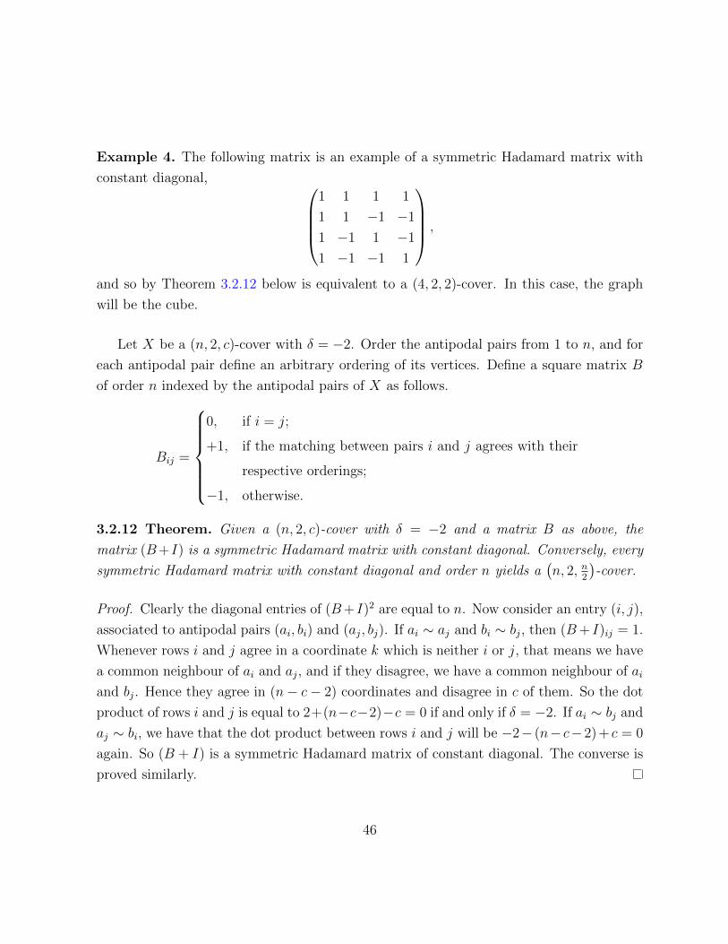
Example 4. The following matrix is an example of a symmetric Hadamard matrix with

constant diagonal, 1 1 1 1

1 1 −1 −1

1 −1 1 −1

1 −1 −1 1

,

and so by Theorem 3.2.12 below is equivalent to a (4, 2, 2)-cover. In this case, the graph

will be the cube.

Let X be a (n, 2, c)-cover with δ = −2. Order the antipodal pairs from 1 to n, and for

each antipodal pair define an arbitrary ordering of its vertices. Define a square matrix B

of order n indexed by the antipodal pairs of X as follows.

Bij =

0, if i = j;

+1, if the matching between pairs i and j agrees with their

respective orderings;

−1, otherwise.

3.2.12 Theorem. Given a (n, 2, c)-cover with δ = −2 and a matrix B as above, the

matrix (B+I) is a symmetric Hadamard matrix with constant diagonal. Conversely, every

symmetric Hadamard matrix with constant diagonal and order n yields a(n, 2, n

2

)-cover.

Proof. Clearly the diagonal entries of (B+I)2 are equal to n. Now consider an entry (i, j),

associated to antipodal pairs (ai, bi) and (aj, bj). If ai ∼ aj and bi ∼ bj, then (B+ I)ij = 1.

Whenever rows i and j agree in a coordinate k which is neither i or j, that means we have

a common neighbour of ai and aj, and if they disagree, we have a common neighbour of ai

and bj. Hence they agree in (n− c− 2) coordinates and disagree in c of them. So the dot

product of rows i and j is equal to 2+(n−c−2)−c = 0 if and only if δ = −2. If ai ∼ bj and

aj ∼ bi, we have that the dot product between rows i and j will be −2− (n− c−2) + c = 0

again. So (B + I) is a symmetric Hadamard matrix of constant diagonal. The converse is

proved similarly.

46

Example 5. Consider the Hadamard matrix of Example 4. Following the steps of the

proof above, we can easily construct the adjacency matrix of the corresponding (4, 2, 2)-

cover as follows. First turn the diagonal entries into 0. Replace these entries by the zero

matrix of dimension two, then replace all entries equal to +1 by I2, and all entries equal

to −1 by A(K2). The resulting matrix is the adjacency matrix of the cube:

0 0 1 0 1 0 1 0

0 0 0 1 0 1 0 1

1 0 0 0 0 1 0 1

0 1 0 0 1 0 1 0

1 0 0 1 0 0 0 1

0 1 1 0 0 0 1 0

1 0 0 1 0 1 0 0

0 1 1 0 1 0 0 0

.

If X is a (n, 2, c)-cover with δ = −2, it follows from arithmetic conditions on the

multiplicities of the eigenvalues of X that n must be a square (see Godsil and Hensel

[37, Lemma 3.7]). This can also be derived as a necessary condition for the existence of

symmetric Hadamard matrices of constant diagonal.

It is also a known fact that Hadamard matrices can only exist when n is 1, 2 or a

multiple of 4 (see for instance BCN [13, Section 1.8]).

3.2.13 Theorem. Every (n, 2, c)-cover with δ = −2 admits perfect state transfer at timeπ√n

. For δ = +2, perfect state transfer occurs if and only if n is divisible by 8, and in that

case it occurs at time π2.

Proof. Let X be a (n, 2, c)-cover with δ = −2, and so n is an even perfect square. Using

Equation 3.3, its set of distinct eigenvalues will be

{n− 1,√n− 1, −1, −

√n− 1}.

Applying Theorem 3.2.3, we see that perfect state transfer will occur at timeπ√n

. If

δ = +2, then the set of distinct eigenvalues is

{n− 1,√n+ 1, −1, −

√n+ 1}.

47

If |n|2 = 2−2, then |(n− 1)− (√n+ 1)|2 = |(n− 1)− (−1)|2, and so perfect state transfer

cannot occur. If |n|2 < 2−2, then it is easy to check that perfect state transfer will occur

at time π2.

Symmetric Hadamard matrices of order n with constant diagonal can be constructed

for every n which is a power of 4 as the iterated Kronecker product of the matrix depicted

in Example 4.

Perfect state transfer was already known for the case δ = −2 (see Godsil [33]), but

unknown for the case δ = +2.

Now we move to the case where δ /∈ {0,−2, 2}. As we saw in Proposition 3.2.11, for

every cover with parameter δ, there exists a corresponding cover with parameter −δ.

3.2.14 Theorem. Let X be a (n, 2, c)-cover, and X2 the corresponding (n, 2, n− c− 2)-

cover. Suppose δ /∈ {0,−2, 2}.

a) If δ ≡ 2 mod 4, then perfect state transfer occurs either in X or in X2 at time π2α

, for

some α which is an odd integer.

b) If δ is odd or a multiple of 4, perfect state transfer does not occur in either X or X2.

Proof. Let ρ > 0 and σ < 0 be the eigenvalues of X which are neither (n− 1) nor −1. Let

mρ and mσ be their corresponding multiplicities, which can be computed in terms of n, r

and c (see Godsil and Hensel [37, Section 3]). Then

mρ −mσ =nδ√∆,

This is a difference of integers, so δ 6= 0 implies that ∆ must be a perfect square. Note that

σ = 12(δ −

√∆) is an algebraic integer, hence an integer. Thus

√∆ − δ is even. Suppose

that ∆ = (2t+ δ)2. The parameter n is now parametrized as n = 1 + t2 + tδ.

Note that if n is odd, then perfect state transfer cannot occur by Theorem 3.2.3. If δ

is odd, then n = δ + 2c + 2 is odd. If t is even, then n is also odd. So suppose δ is even

and t is odd.

48

If δ is a multiple of 4, then n = 1 + t2 + tδ ≡ 2 mod 4. Perfect state transfer occurs

only if (n− 1)− ρ and (n− 1)− σ are both odd. Hence ρ and σ are both even. But note

that σ = −t and t is odd.

If δ ≡ 2 mod 4, then n = 1+t2 +tδ ≡ 0 mod 4. Let ρ2 > 0 and σ2 > 0 be the non-trivial

eigenvalues of X2. Note that:

ρ = δ + t and σ = −t,

and

ρ2 = t and σ2 = −δ − t.

If t ≡ 3 mod 4, then (n− 1)− (δ+ t) and (n− 1) + t are both congruent to 2 modulo 4,

so by Theorem 3.2.3 perfect state transfer occurs in X at time π2α

, where 2α is the greatest

common divisor of the differences of the eigenvalues of X. If t ≡ 1 mod 4, then (n− 1)− tand (n−1)− (−δ− t) are both congruent to 2 modulo 4, so perfect state transfer occurs in

X2 at time π2α

, where 2α is the greatest common divisor of the differences of the eigenvalues

of X2.

Note that in the case where δ ≡ 2 mod 4, the theorem above implies that perfect state

transfer occurs in at least one of X and X2. It is possible that perfect state transfer occurs

in both, but in that case it will be at different times.

Table 3.1 below contains parameter sets for which a corresponding cover admits per-

fect state transfer, for n < 280. The strongly regular graph on the first neighbourhood

of a vertex in each of these covers is given in the rightmost column. We consult Andries

Brouwer’s website (http://www.win.tue.nl/∼aeb/graphs/srg/srgtab.html) to either pro-

vide a construction for such a graph, hence a construction for the cover, or to state that

no such construction is known.

49

Table 3.1: Perfect state transfer in distance-regular graphs of diameter 3.

n c δ time construction of strongly regular graph

28 10 6 π/2 complement of Schlafli graph

76 42 −10 π/2 not known

96 40 14 π/4 not known

96 54 −14 π/6 not known

120 54 10 π/6 complement of O−(8, 2) polar graph

136 70 −6 π/2 complement of O+(8, 2) polar graph

148 66 14 π/2 not known

176 72 30 π/4 complement of the one below

176 102 −30 π/2 line graph of Hoffman-Singleton graph

244 130 −18 π/2 not known

276 162 −50 π/6 complement of McLaughlin graph McL.2 / U4(3).2

3.2.3 Larger diameter

We do not analyse this case in the same detail as we did for the diameter three case. The

reason is that the known constructions of antipodal distance-regular graphs of diameter

> 3 are scarcer, and so we prefer to just exhibit which known graphs admit perfect state

transfer. The work in this subsection is due to Coutinho et al. [21].

The results below are straightforward corollaries of Theorem 3.2.3. We refer to BCN

[13, Chapters 9, 11 and 13] for the definition and further details of the graphs mentioned

in them.

3.2.15 Corollary. The graphs below are examples of distance-regular graphs of diameter

larger than three admitting perfect state transfer.

(i) Hamming d-cubes. Number of vertices: 2d. Valency: d. Diameter: d. Distinct

eigenvalues: {d− 2i : i = 0, ..., d}. Time of perfect state transfer: π2.

50

(ii) Halved 2d-cubes. Number of vertices: 22d−1. Valency:(

2d2

). Diameter: d. Distinct

eigenvalues:{(

2d2

)− 2i(2d− i) : i = 0, ..., d

}. Time of perfect state transfer: π

2.

(iii) Hadamard graphs2 of order n if and only if n is a perfect square. Exist for infinitely

many values of n, in particular for all n which are powers of 4. Number of vertices:

4n. Valency: n. Diameter: 4. Time of perfect state transfer: π√n

.

(iv) Meixner graph (Martin et al. [58, Example 3.5]). Number of vertices: 1344. Valency:

176. Diameter: 4. Distinct eigenvalues: {176, 44, 8,−4,−16}. Time of perfect state

transfer: π12

.

(v) Coset graph of the once shortened and once truncated binary Golay code. Number of

vertices: 1024. Valency: 21. Diameter: 6. Distinct eigenvalues: {21, 9, 5, 1,−3,−7,−11}.Time of perfect state transfer: π

4.

(vi) Coset graph of the shortened binary Golay code. Number of vertices: 2048. Valency:

22. Diameter: 6. Distinct eigenvalues: {22, 8, 6, 0,−2,−8,−10}. Time of perfect

state transfer: π2.

(vii) Double coset graph of truncated binary Golay code. Number of vertices: 2048. Va-

lency: 22. Diameter: 7. Distinct eigenvalues: {22, 10, 6, 2,−2,−6,−10,−22}. Time

of perfect state transfer: π4.

(viii) Double coset graph of binary Golay code. Number of vertices: 4096. Valency: 23.

Diameter: 7. Distinct eigenvalues: {23, 9, 7, 1,−1,−7,−9,−23}. Time of perfect

state transfer: π2.

3.2.16 Corollary. No graph in the following infinite families of antipodal distance-regular

graphs with classes of size two admits perfect state transfer.

(i) Johnson graphs J(2n, n) for n > 1. Their distinct eigenvalues are {(n − j)2 − j},with j ∈ {0, ..., n}.

(ii) Doubled odd graphs on 2n+1 points. Their distinct eigenvalues are {(−1)j(n+1−j)},with j ∈ {0, 1, ..., n− 1, n, n+ 2, n+ 3, ..., 2n+ 2}.

2These are not those mentioned in Subsection 3.2.2.

51

We also checked graphs with diameter larger than 3 depicted in tables of BCN [13,

Chapter 14] that do not belong to the infinite families above.

3.2.17 Corollary. None of the following antipodal distance-regular graphs with classes of

size two and diameter larger than three admit perfect state transfer.

(i) Wells graph of diameter 4. Some eigenvalues are not integral.

(ii) Double Hoffman-Singleton Graph of diameter 5. Distinct eigenvalues are {7, 3, 2,−2,

− 3,−7}.

(iii) Double Gewirtz Graph of diameter 5. Distinct eigenvalues are {10, 4, 2,−2,−4,−10}.

(iv) Double 77-Graph of diameter 5. Distinct eigenvalues are {16, 6, 2,−2,−6,−16}.

(v) Double Higman-Sims Graph of diameter 5. Distinct eigenvalues are {22, 8, 2,−2,−8,

− 22}.

(vi) Dodecahedron of diameter 5. Distinct eigenvalues are not integer.

3.3 Perfect state transfer on association schemes

Consider an association scheme {A0, ..., Ad}. Any sum of distinct Schur idempotents is

a 01-matrix and in particular defines a graph. We recall that we say that such a graph

belongs to the association scheme. Our intent in this section is to construct new examples

of perfect state transfer among such graphs.

3.3.1 Proposition. If A and B are commuting matrices, then

exp(it(A+B)) = exp(itA) exp(itB).

We also recall two important facts in the following corollary (see Theorems 2.4.3 and

3.2.1).

52

3.3.2 Corollary. If X is a graph belonging to an association scheme admitting perfect

state transfer at time τ , then

a) U(τ) is a multiple of a permutation matrix of order two and no fixed points that belongs

to the Bose-Mesner algebra of the scheme; and

b) the eigenvalues of X are integers, and therefore τ = πg

for some integer g.

As a consequence, we can construct new examples of graphs admitting perfect state

transfer based on old examples.

3.3.3 Corollary. Suppose X is a graph belonging to an association scheme admitting

perfect state transfer at time τ = πg

with phase λ. Let A = A(X). Say U(τ) = λT . Let B

be a 01-matrix belonging to the scheme satisfying the following properties.

a) The 1s of B are in disjoint positions from those of A.

b) The eigenvalues of B are integers.

c) Either |θ|2 = |g|2 for all eigenvalues θ of B, or |θ|2 < |g|2 for all eigenvalues θ of B.

Then A+B is the adjacency matrix of a graph, and UA+B(τ) = λ′T , where λ′ = ±λ.

Proof. From a), A + B is the adjacency matrix of a graph. Conditions b) and c) imply

that

UB(τ) = ±I,

and so from Proposition 3.3.1, we have

UA+B(τ) = UA(τ)UB(τ) = ±λT.

A standard way of constructing association schemes is using the tensor product of

matrices. We explain below.

53

Consider two association schemes {A0, ..., Ad} and {B0, ..., Be}. The set of matrices

obtained by taking the Kronecker product of the matrices in both schemes

{Ai ⊗Bj : 0 ≤ i ≤ d and 0 ≤ j ≤ e}

is an association scheme with (de + d + e) classes (see Bailey [6, Chapter 3]). It is the

tensor product of the original schemes.

The direct product3 of graphs X and Y is defined to be the graph with adjacency

matrix A(X) ⊗ A(Y ), and is usually denoted by X × Y . In Chapter 4, we will readdress

the problem of characterizing perfect state transfer in graph products in a more general and

detailed framework. Here we will present a particular case that provides a good number

of examples of graphs belonging to association schemes admitting perfect state transfer.

The direct product of a graph X with K2 is also referred to as the bipartite double

of X. If X is distance-regular, X × K2 belongs to the tensor product of the schemes

{I, A(X), A2(X), ...., Ad(X)} and {I2, A(K2)}.

3.3.4 Theorem. Let V (K2) = {v1, v2}. Suppose X is distance-regular on n vertices with

eigenvalues θ0 > ... > θd, and let θr = 2fr`r, where `r is an odd integer. For any vertex

u ∈ V (X), the graph X×K2 admits perfect state transfer between (u, v1) and (u, v2) if and

only if both conditions hold:

(i) For all r, we have fr = a for some constant a.

(ii) For all r and s, we have `r ≡ `s mod 4.

Under these conditions, perfect state transfer occurs at time π2 gcd{θ0,...,θd}

.

Proof. It follows from the definition of direct product that the eigenvalues of X ×K2 are

±θi. Note that the matrix In ⊗ A(K2) is a permutation matrix of order two having no

fixed points, and that

(In ⊗ A(K2))(E+θi) = E+θi and (In ⊗ A(K2))(E−θi) = −E−θi .

Condition (iii) of Theorem 2.4.4 is equivalent to the two conditions below. Here g is the

gcd of the differences of the eigenvalues of X ×K2.

3See Section 4.2.

54

(1) |θr − θs|2 < |g|2 for all r and s; and

(2) |θr − (−θs)|2 = |g|2 for all r and s.

If r = s, then (2) is equivalent to Condition (i) of the statement. Assuming Condition (i),

(1) and (2) are equivalent to

(1’) `r−`s2

even, for all r and s; and

(2’) `r+`s2

odd, for all r and s.

which is equivalent to Condition (ii). The time follows from the expression for time given

in Theorem 2.4.4.

The following corollaries are due to Coutinho et al. [21], and they exhibit some new

examples of perfect state transfer. Note that the distance between vertices involved in

perfect state transfer in these examples is the odd girth of the graph. The definition of

these graphs can be found in Godsil and Royle [42, Chapter 10] for strongly regular graphs

or in BCN [13] for distance-regular graphs. For generalized quadrangles, a more detailed

account can be found in [61].

3.3.5 Corollary. The following bipartite doubles of strongly regular graphs admit perfect

state transfer.

(i) Bipartite doubles of the point graphs of generalized quadrangles GQ(s, t) whenever q

is a prime power and one of the following conditions hold:

s = q − 1, t = q + 1 with q ≡ 0 mod 4,

s = q, t = q2 with q ≡ 7 mod 8,

s = q3, t = q2 with q ≡ 7 mod 8,

t = 1 , with s ≡ 7 mod 8.

Number of vertices: 2(st+ 1)(s+ 1). Valency: s(t+ 1). Perfect state transfer at π4.

55

(ii) Bipartite doubles of the complements of the point graphs of generalized quadrangles

GQ(s, t) whenever q is a prime power and one of the following conditions hold:

s = q, t = q2, with q ≡ 3 mod 4: perfect state transfer at π2q

,

s = q2, t = q, with q ≡ 3 mod 4: perfect state transfer at π2q

,

s = q − 1, t = q + 1, with q even : perfect state transfer at π2,

s = q + 1, t = q − 1, with q even: perfect state transfer at π2,

s = q2, t = q3, with q ≡ 3 mod 4: perfect state transfer at π2q2

,

s = q3, t = q2, with q ≡ 3 mod 4: perfect state transfer at π2q2

.

Number of vertices: 2(st+ 1)(s+ 1). Valency: s2t.

(iii) Bipartite doubles of orthogonal array graphs OA(n,m) if |n|2 ≤ |m|24

. Number of

vertices: 2n2. Valency: m(n− 1). Perfect state transfer at 2πgcd(n,4m)

.

(iv) Bipartite doubles of complements of orthogonal array graphs OA(n,m) if |n|2 ≤ m−1|24

.

Number of vertices: 2n2. Valency: n2 − m(n − 1) − 1. Perfect state transfer at2π

gcd(n,4(m−1)).

3.3.6 Corollary. The following bipartite doubles of distance-regular graphs with classical

parameters admit perfect state transfer.

(i) Bipartite doubles of Grassmann graphs Jq(n, d) (n ≥ 2d) for n even, d odd and

q ≡ 3 mod 4. Classical parameters:(d, q, q, q q

n−d−1q−1

). Perfect state transfer at π

2.

(ii) Bipartite doubles of Hamming graphs H(d, q) when |q|2 ≤ |4d|2. Classical parameters:

(d, 1, 0, q − 1). Perfect state transfer at 2πgcd(q,4d)

.

(iii) Bipartite doubles of Doob graphs of odd diameter. Classical parameters: (d, 1, 0, 3).

Perfect state transfer at π2.

(iv) Bipartite doubles of unitary dual polar graphs 2A2d−1(q) and 2A2d(q), both cases when

|q + 1|2 ≤ |4d|2. Classical parameters: (d, q2, 0, q) and (d, q2, 0, q3), respectively. Per-

fect state transfer at 2πgcd(q+1,4d)

.

56

(v) Bipartite doubles of parabolic and symplectic dual polar graphs Bd(q) and Cd(q) when

q ≡ 3 mod 4 and d is odd. Classical parameters: (d, q, 0, q). Perfect state transfer atπ2.

(vi) Bipartite doubles of half dual polar graph of diameter d on 2d-spaces when |q +

1|2 ≤ |4d|2. Classical parameters:(d, q2, q2 + q, q q

2d−1−1q−1

). Perfect state transfer

at π2 gcd(d,q+1)

.

(vii) Bipartite doubles of half dual polar graph of diameter d on 2d + 1-spaces when |(q +

1)(q2 + 1)|2 ≤ |4d|2. Classical parameters:(d, q2, q2 + q, q q

2d+1−1q−1

). Perfect state

transfer at2π

gcd(

(q + 1)(q2 + 1), 4 q2d+1−1q2−1

q2d−1q−1

) .(viii) Bipartite doubles of exceptional graphs of Lie type when q ≡ 11 mod 12 or when

q ≡ 3, 7 mod 12. Classical parameters:(

3, q4, q q4−1q−1

, q q9−1q−1

). In the first case, perfect

state transfer at time π6. In the second, at time π

2.

(ix) Bipartite doubles of all affine E6 graphs when q is even. Classical parameters: (3, q4, q4−1, q9 − 1). Perfect state transfer at π

2.

(x) Bipartite doubles of all alternating forms graphs when q is even. Classical parameters:

(d, q2, q2 − 1, q2d−1 − 1) and (d, q2, q2 − 1, q2d+1 − 1) for forms on 2d- and on 2d+ 1-

spaces, respectively. Perfect state transfer at π2.

(xi) Bipartite doubles of all Hermitian forms graphs when q is even. Classical parameters:

(d,−q,−q − 1,−(−q)d − 1). Perfect state transfer at π2.

57

Chapter 4

Graph products and double-covers

This chapter examines in detail how perfect state transfer in certain graph products relates

to properties of the factors. The methods we introduce in this chapter can be used to study

state transfer in graphs whose adjacency matrix is a sum of Kronecker products of matrices.

First, we present an overview of our methods, restricting to the case in which the

adjacency matrix of the graph X is of the form

A(X) = B ⊗ C +M ⊗N

with B,C,M,N symmetric matrices. All significant examples we have are graphs of this

form.

Following this, we study in detail perfect state transfer in the direct product of graphs.

This problem was studied by Ge et al. [31]. In particular, they showed that X × H

admits perfect state transfer if X admits perfect state transfer at a time τ , τθπ∈ Z for all

eigenvalues θ of X, and H is a circulant graph with odd eigenvalues. Here we will generalize

their work. On one hand, we first show that if X × Y admits perfect state transfer, then

at least one of the factors must admit perfect state transfer (similarly to what happens

with the Cartesian product of graphs). On the other hand, we show that the hypothesis

on the other factor can be significantly weakened, in particular, H need not be a circulant

nor have odd eigenvalues. For example, we show that under somewhat similar integrality

58

conditions on the eigenvalues, if X admits perfect state transfer and the 2-adic norm of

the integer part of the eigenvalues of Y is constant, then X�k ⊗ Y admits perfect state

transfer for some sufficiently large values of k.

We then proceed to show how our methods can be used in other notions of graph

products, in particular, we will show that the sufficient condition for perfect state transfer in

the lexicographic product of regular graphs presented by Ge et al. [31] is also necessary. We

will also show that perfect state transfer in the strong product of graphs can be determined

using the same methods we used for the direct product.

Finally, we will apply our methods to graphs which are double-covers of other graphs,

focusing on double-covers of the complete graph. Here we will find new examples of perfect

state transfer.

4.1 Framework for studying state transfer in products

In this section, we will introduce a very general method for determining whether perfect

state transfer is possible in graphs which are sums of tensor products of 01-matrices. For

the purpose of simplifying the notation, we will restrict our considerations to graphs X

such that

A(X) = B ⊗ C +M ⊗N

with B,C,M,N symmetric matrices, but both the number of terms of the sum and the

number of factors in each term can be generalized to any positive integer, as we will see in

Section 4.3.

Definition. The Cartesian product of graphs X and Y is denoted by X�Y and is defined

as the graph with adjacency matrix

A(X�Y ) = A(X)⊗ I + I⊗ A(Y ).

It can be defined combinatorially as follows. Its vertex set is V (X�Y ) = V (X)× V (Y ),

and (u1, v1) ∼ (u2, v2) if and only if either u1 = u2 and v1v2 ∈ E(Y ), or v1 = v2 and

u1u2 ∈ E(X). Thus A(X�Y ) and A(Y�X) define the same graph.

59

4.1.1 Theorem (Christandl et al. [20]). If X and Y are graphs, then, for all t, we have

UX�Y (t) = UX(t)⊗ UY (t). (4.1)

We will later present a proof of Theorem 4.1.1, but note that it implies the following

corollary trivially.

4.1.2 Corollary. For graphs X and Y , the graph X�Y admits perfect state transfer at

time τ if and only if either of the graphs admits perfect state transfer at time τ , and if only

one of them does, the other must contain a vertex which is periodic at time τ .

When we introduced the spectral decomposition of a matrix, we assumed the projectors

Er represent projections onto the eigenspaces, and therefore their ranks are equal to the

multiplicity of the corresponding eigenvalues. Now we consider a refinement of such a

decomposition. If M is a symmetric m×m matrix, M admits a decomposition into rank-1

orthogonal projectors

M =m−1∑r=0

θrEr. (4.2)

Here we are no longer requiring that θr 6= θs if r 6= s. Note that if {v0, ...,vm−1} forms an

orthonormal basis of eigenvectors of M , then we can choose Er = vrvTr .

For the lemmas below, suppose X is such that A(X) = B ⊗ C + M ⊗ N . We require

B and M to be m×m matrices, and C and N to be n× n matrices. Because of that, we

identify the rows and columns of B and M , similarly for C and N . A typical vertex of X

will be represented as (w, u), where w indexes a row of B and M , and u a row of C and N .

Further to that, suppose that B and M commute. Let β0 ≥ ... ≥ βm−1 and µ0 ≥ ... ≥ µm−1

be the spectra of B and M respectively, and γ0 ≥ ... ≥ γn−1 and ν0 ≥ ... ≥ νn−1 be the

spectra of C and N respectively.

4.1.3 Lemma. Suppose X is as above. Then UX(t) is similar to a block diagonal matrix

with m blocks, in which each block is of the form exp(itLr), with

Lr = βrC + µrN.

60

Proof. By Theorem 2.1.8, and because B and M are symmetric and commute, there exists

an orthogonal matrix P such that P TBP and P TMP are diagonal. Hence we have that

L = (P T ⊗ I) (B ⊗ C +M ⊗N) (P ⊗ I)

is a block diagonal matrix whose blocks are equal to Lr = βrC + µrN . The result now

follows from the fact that

UL(t) = (P T ⊗ I) UX(t) (P ⊗ I).

In the context of the lemma above, we recall that we can use the terms perfect state

transfer and periodicity with respect to symmetric matrices in general.

4.1.4 Lemma. Suppose X is as above, and let E0, ..., Em−1 be the rank-1 projectors onto

the common eigenspaces of B and M . Let Lr = βrC +µrN . If the graph X admits perfect

state transfer from (w, u) to (z, v), then

(i) the vertices (column indices) w and z are strongly cospectral in the matrices B and

M ; and

(ii) for all r such that Erw 6= 0; if u = v, the matrix Lr is periodic at u; and if u 6= v,

the matrix Lr admits perfect state transfer from u to v.

Proof. By hypothesis, there exists a time τ and a complex number λ such that

UX(τ)(ew ⊗ eu) = λ(ez ⊗ ev).

Let P be the matrix that simultaneously diagonalizes B and M . Hence

(P T ⊗ I)UX(τ)(ew ⊗ eu) = λ(P Tez ⊗ ev),

and thus, by Lemma 4.1.3,eiτL0

eiτL2

. . .

eiτLm−1

(P Tew ⊗ eu) = λ(P Tez ⊗ ev).

61

This is true if and only if, for all r = 0, ...,m− 1,

(eTr PTew)eiτLreu = (eTr P

Tez)λev.

Because the matrices eitLr are all unitary, it follows that, for all r,

(eTr PTew) = ±(eTr P

Tez),

and so w and z are strongly cospectral in the matrices B and M ; and also that

eiτLreu = ±λev

for all r such that (eTr PTew) 6= 0.

4.1.5 Lemma. Suppose X is as above, and now with the extra assumption that C and N

also commute. Let F0, ..., Fn−1 be the common rank-1 projectors for C and N . Then

UX(t) =m−1∑r=0

n−1∑s=0

eit(βrγs+µrνs)Er ⊗ Fs.

Proof. Note that

B ⊗ C +M ⊗N =m−1∑r=0

n−1∑s=0

(βrγs + µrνs)Er ⊗ Fs.

From

UX(t) = exp(it(B ⊗ C +M ⊗N

)),

and the facts that BM = MB and CN = NC, it follows that

UX(t) =m−1∑r=0

n−1∑s=0

eit(βrγs+µrνs)Er ⊗ Fs.

62

4.2 Direct product of graphs

Consider graphs X and Y with respective adjacency matrices A(X) and A(Y ).

Definition. We recall that the direct product of X and Y , denoted by X×Y , is the graph

with adjacency matrix A(X)⊗ A(Y ).

It can be defined combinatorially as follows. Its vertex set is V (X × Y ) = V (X)× V (Y ),

and (u1, v1) ∼ (u2, v2) if and only if u1u2 ∈ E(X) and v1v2 ∈ E(Y ). Thus A(X) ⊗ A(Y )

and A(Y )⊗ A(X) define the same graph.

This product is also known in the literature as the weak direct product, the tensor

product, the categorical product, and many other names (see Hammack et al. [46, Chapter

4]). In this section, we study when a direct product of graphs admits perfect state transfer.

As an immediate application, we find more examples of perfect state transfer.

4.2.1 Theorem. Suppose X and Y are graphs, and X × Y admits perfect state transfer

between vertices (w, u) and (z, v). If u = v, then Y is periodic at u. If u 6= v, then Y

admits perfect state transfer between u and v. Likewise, if w = z, then X is periodic at w.

If w 6= z, then X admits perfect state transfer between w and z.

Proof. It is a simple consequence of Lemma 4.1.4 with B = C = O, M = A(X) and

N = A(Y ), or M = A(Y ) and N = A(X).

4.2.2 Lemma. Suppose X and Y are graphs and A(X) admits the spectral decomposition

A(X) =d∑r=0

θrEr. Then

UX×Y (t) =d∑r=0

Er ⊗ UY (θrt).

Proof. It is a consequence of Lemma 4.1.5 and an easy rearrangement.

Now we will show under which conditions on the factors we can obtain perfect state

transfer on the product.

63

4.2.3 Theorem. Suppose UY (τ)eu = λev, and that the eigenvalues of Y in the support of u

are of the form bi√

∆u. Suppose w and z are strongly cospectral vertices in X. Then X⊗Yadmits perfect state transfer from (w, u) to (z, v) if and only if the following conditions hold.

(i) For all θr ∈ Φw, we have θr = tr√

∆w, where tr ∈ Z and ∆w is a square-free positive

integer (which could be 1).

(ii) The 2-adic norms of tr are all the same.

(iii) If λ is a primitive n-th root of the unit, then n is even, and there exists an integer m

such that

a) If θr ∈ Φ+wz, then the odd part of tr is congruent to m modulo n.

b) If θr ∈ Φ−wz, then the odd part of tr is congruent to m+ n2

modulo n.

Proof. Let Φw = {θ0, ..., θd}, and Φu = {ϕ0, ..., ϕk}. Let h be the gcd of the differences

(ϕ0 − ϕr) for r = 1, ..., k. Let h = 2e`, with ` an odd integer.

Suppose that perfect state transfer occurs in X×Y between (w, u) and (z, v) at time τ

and phase γ. As a consequence of the fact that A(X×Y ) = A(X)⊗A(Y ), the eigenvalues

in the support of (w, u) are of the form θrϕi, with 0 ≤ r ≤ d and 0 ≤ i ≤ k. In light of

Theorem 2.4.3, the eigenvalues θr are either integers or integer multiples of√

∆w for some

square-free positive ∆w ∈ Z.

Then, using Lemma 4.2.2, we have

γ(ez ⊗ ev) = UX⊗Y (τ)(ew ⊗ eu)

=d∑r=0

(Er ⊗ UY (θrτ))(ew ⊗ eu)

=d∑r=0

Erew ⊗ UY (θrτ)eu.

Multiplying both sides by Er ⊗ I, we get that, for σr ∈ {+1,−1},

UY (θrτ)eu = σrγev

64

depending on whether θr ∈ Φ+wz of θr ∈ Φ−wz. In either case, θrτ is a time for which perfect

state transfer occurs in Y between u and v. Applying Theorem 2.4.4, this implies that

θrτ = `rπ

2e.`√

∆u

and σrγ = λ`r ,

where `r is an odd integer. Considering θr and θs in the support of w, we will have

θrθs

=`r`s. (4.3)

Because the integers `r are odd, the 2-adic norm of each tr is the same, proving (ii).

To prove condition (iii), suppose we take m′ ∈ {1, ..., n} such that λm′

= γ. The fact

that there is a m′′ such that λm′′

= −γ is equivalent to (−1) being a power of λ, which

happens if and only if n is even. In that case, if θr ∈ Φ+wz, then `r ≡ m′ mod n, and if

θr ∈ Φ−wz, then `r ≡ m′+ n2

mod n. Note that the odd part of tr is an odd multiple `r, which

by Equation 4.3 does not depend on r. Say `′. So if the integers `r satisfy the congruences

with m′, so will the odd parts of tr with m = m′`′.

Now suppose all three conditions hold. Let tr = 2f .kr, for some f ≥ 0 and odd integers

kr. By Lemma 4.2.2, we have

UX×Y

(π

2e+f`√

∆w

√∆u

)=

d∑r=0

Er ⊗ UY(θr.

π

2e+f`√

∆w

√∆u

).

Note that

UY

(θr.

π

2e+f`√

∆w

√∆u

)= UY

(kr

π

2e`√

∆u

)=

[UY

(π

2e`√

∆u

)]krHence

UX×Y

(π

2e+f`√

∆w

√∆u

)(ew ⊗ eu) =

d∑r=0

Erew ⊗[UY

(π

2e√

∆u

)]kreu

=d∑r=0

Erew ⊗ λkrev.

65

If r ∈ Φ+wz, then condition (iii) implies that λkr = λm, and if r ∈ Φ−wz, then λkr = λ−m. If

λm = γ, we have

UX×Y

(π

2e+f√

∆w

√∆u

)(ew ⊗ eu) = γ(ez ⊗ ev),

as claimed.

Note that if w = z, the theorem above takes the following form.

4.2.4 Corollary. Suppose UY (τ)eu = λev, and that the eigenvalues of Y in the support of

u are of the form bi√

∆u. Let w ∈ V (X). Then X × Y admits perfect state transfer from

(w, u) to (w, v) if and only if the following conditions hold.

(i) For all θr ∈ Φw, we have θr = tr√

∆w, where tr ∈ Z and ∆w is a square-free positive

integer (which could be 1).

(ii) The 2-adic norms of tr are all the same.

(iii) If λ is a primitive n-th root of the unit, then there exists an integer m such that the

odd part of the integer tr is congruent to m modulo n.

We draw the reader’s attention to the following fact. The conditions on X of both

results depend very little on Y . In fact, if ϕ0 is the largest eigenvalue of Y and τ is the

time at which perfect state transfer occurs in Y , then the three conditions depend only on

the eigenvalues of X, with the exception of the order of eiϕ0τ as a root of unity. This fact

can be explored in the following corollary.

4.2.5 Corollary. If X×Y admits perfect state transfer, and if the eigenvalues of Y in the

support of the vertices involved in perfect state transfer are integers or integer multiples of

a square root, then X × Y �k admits perfect state transfer for all k ∈ Z+.

Proof. By Theorem 4.1.1, if Y admits perfect state transfer at minimum time τ , then

so does Y �k at the same time. Moreover, if the largest eigenvalue of Y is ϕ0, then the

largest eigenvalue of Y �k is kϕ0. Hence the order of the phase of state transfer in Y �k

66

either decreases or stays the same. If it decreases by an odd factor, nothing changes. If

it decreases by an even factor, then what could happen is that X × Y admits perfect

state transfer between (w, u) and (z, v) and X×Y �k admits perfect state transfer between

(w, u, u, ..., u) and (w, v, v, ..., v), and between (z, u, u, ..., u) and (z, v, v, ..., v).

This can be pushed even further.

4.2.6 Corollary. If Y admits perfect state transfer, if the eigenvalues of X and Y are

integers or integer multiples of a square root, and if the 2-adic norm of the integer parts of

the eigenvalues of X are all the same, then there exists a k0 ∈ Z+ such that X ⊗ Y �(mk0)

admits perfect state transfer for all m ≥ 1.

As a consequence, we present new examples of perfect state transfer in simple graphs.

For the cases below, we assume that Y is a graph admitting perfect state transfer between

u and v, and that the eigenvalues of Y in the support of u are either integers or integer

multiples of square roots. All the graphs known in the literature admitting perfect state

transfer are of this form.

Example 6 (Stars). Let Sn represent the graph on n + 1 vertices with degree sequence

(n, 1, 1, ..., 1). The spectrum of Sn is

{√n

(1), 0(n−2), −

√n

(1)}.

Let w be the vertex of degree n. The eigenvalue support of w is {√n,−√n}.

From Corollary 4.2.6, there is a k such that Sn×Y �k admits perfect state transfer from

(w, u, u, ..., u) to (w, v, v, ..., v).

Note that k is usually quite small. If Y admits perfect state transfer at time π2, which

is a rather common situation, then k = 2 will suffice.

Example 7 (Odd eigenvalues). If X is a graph with odd eigenvalues, and w ∈ V (X),

then it follows from Corollary 4.2.6 that there is a k such that X × Y �k admits perfect

state transfer from (w, u, u, ..., u) to (w, v, v, ..., v).

67

We can find many graphs with odd eigenvalues among the known distance-regular

graphs. For example, there are 32548 non-isomorphic strongly regular graphs with param-

eters (36,15,6,6). These graphs have eigenvalues {15, 3,−3}. The tensor product of each

of them with C4 will admit perfect state transfer.

4.3 Other graph products

We list some examples of traditional graph products below. See Hammack et al. [46] for

the combinatorial definitions.

1) The lexicographic product X o Y satisfies

A(X o Y ) = A(X)⊗ J + I⊗ A(Y ).

2) The strong graph product X � Y satisfies

A(X � Y ) = A(X)⊗ [A(Y ) + I] + I⊗ A(Y ).

3) The modular product X � Y satisfies

A(X � Y ) = A(X)⊗ [A(Y ) + I] + I⊗ A(Y ) + A(X)⊗ A(Y ).

The matrix A(X) commutes with I, and so we can use the technology from Section 4.1

to analyse cases 1) and 2). Our technology could also be applied to study case 3) if we

assume that either X or Y is regular.

For the lexicographic product X oY , we further suppose that Y and J commute, which

is equivalent to Y being a k-regular graph. If A(X) and A(Y ) admit decompositions into

rank-1 projectors

A(X) =n−1∑r=0

θrEr and A(Y ) =k

mJ +

m−1∑s=1

ρsFs,

68

then it follows from Lemma 4.1.5 that

UXoY (t) =n−1∑r=0

(eit(θrm+k)Er ⊗

1

mJ +

m−1∑s=1

eitρsEr ⊗ Fs

),

and so

UXoY (t) = UX(mt)⊗ eitk

mJ + I⊗

(UY (t)− eitk

mJ

). (4.4)

In Ge et al. [31, Lemma 5], sufficient conditions for perfect state transfer in X o Y when Y

is regular are presented. Here we characterize perfect state transfer in this context.

4.3.1 Theorem. Suppose X and Y are graphs, and Y is k-regular on m vertices, m > 1.

Then X o Y admits perfect state transfer from (u,w) to (v, z) at time τ and with phase λ

if and only the conditions below hold.

(i) X is periodic at u at time mτ with a phase γ.

(ii) The vertices w and z are distinct and strongly cospectral in Y .

(iii) The following equality holds γeiτk = λ.

(iv) For all s ∈ {1, ...,m− 1}, we have eiτρsFsew = λFsez.

Proof. By Equation 4.4, UXoY (τ)(eu ⊗ ew) = λ(ev ⊗ ez) if and only if

(UX(mτ)− I)eu ⊗eiτk

mj + eu ⊗ UY (τ)ew = λ(ev ⊗ ez).

This is equivalent to having eu = ev, and to existing a γ such that UX(mτ)eu = γeu and

UY (τ)ew = λez −(γ − 1)

meiτkj.

This equality above is true if and only if the projections of both sides on each eigenspace

of A(Y ) are equal. For the eigenspaces that do not correspond to the eigenvalue k, the

projections are equal if and only if conditions (ii) and (iv) hold. The projections onto the

eigenspace corresponding to k are equal if and only if

(γ − 1)eiτk + eiτk = λ,

or equivalently γeiτk = λ.

69

Example 8. Using the result above, we can construct a new example of perfect state

transfer. Consider the lexicographic product K2 o (mK2) with m odd. In this case, τ = π2,

γ = −1 and λ = −1.

For the strong graph product, we have the following.

4.3.2 Proposition. If X and Y are graphs, and A(X) =∑d

r=0 θrEr is the spectral de-

composition of A(X) with θr varying among its distinct eigenvalues, we have:

UX�Y (t) =d∑r=0

eiθrtEr ⊗ UY ((θr + 1)t).

Proof. We split the expression for the strong product as

A(X � Y ) = A(X)⊗ I + I⊗ A(Y ) + A(X)⊗ A(Y ),

or even

A(X � Y ) = A(X�Y ) + A(X × Y ).

Thus

UX�Y (t) = UX�Y (t) · UX×Y (t),

and hence, using Lemma 4.2.2 and Theorem 4.1.1,

UX�Y (t) =(UX(t)⊗ UY (t)

)( d∑r=0

Er ⊗ UY (θrt))

=d∑r=0

eiθrtEr ⊗ UY ((θr + 1)t).

The corollary below is an analogous version of Theorem 4.2.1 and it is a straightforward

consequence of Lemma 4.1.4.

4.3.3 Corollary. Suppose X and Y are graphs, A(X) =∑d

r=0 θrEr, and X � Y admits

perfect state transfer between vertices (w, u) and (z, v). If u = v, then Y is periodic at u.

If u 6= v, then Y admits perfect state transfer between u and v. Likewise, if w = z, then

X is periodic at w. If w 6= z, then X admits perfect state transfer between w and z.

70

Moreover, analogous results to Theorem 4.2.3 and Corollary 4.2.4 could be written in

this case, but with more complicated expressions.

4.4 Double-covers and switching graphs

Definition. Given graphs X and Y on the same set of vertices, we define the graph XnYas the graph with adjacency matrix

A(X n Y ) =

(A(X) A(Y )

A(Y ) A(X)

).

If A(X) ◦A(Y ) = O, then X n Y is a double cover of the graph with adjacency matrix

A(X) +A(Y ). When A(Y ) = J− I−A(X), then X n Y is a double cover of the complete

graph and is known in the literature as the switching graph of X (see Godsil and Royle

[42, Chapter 11]).

If X is the empty graph, then X n Y = A(K2) ⊗ A(Y ) is the bipartite double of Y .

We studied perfect state transfer on bipartite doubles of graphs belonging to association

schemes in Section 3.3. Here we intend to study X n Y in a more general form.

Note that I2 and A(K2) commute, and can be simultaneously diagonalized by

H =1√2

(1 1

1 −1

).

Using Lemma 4.1.3, we have the following lemma.

4.4.1 Lemma. Given graphs X and Y , with A = A(X) and B = A(Y ), we have, for all

t,

(H ⊗ I)UXnY (t)(H ⊗ I) =

(UA+B(t) 0

0 UA−B(t)

).

4.4.2 Theorem. Given graphs X and Y on the same vertex set V , with A = A(X) and

B = A(Y ), the graph X n Y on vertex set {0, 1} × V admits perfect state transfer if and

only if, for some τ ∈ R+ and u ∈ V ,

λ = [UA+B(τ)]u,u = −[UA−B(τ)]u,u and |λ| = 1.

71

In that case, perfect state transfer is between (0, u) and (1, u).

Proof. From Lemma 4.4.1, it follows that

UXnY (t) =1

2

(UA+B(t) + UA−B(t) UA+B(t)− UA−B(t)

UA+B(t)− UA−B(t) UA+B(t) + UA−B(t)

).

For any u ∈ V , if perfect state transfer happens at τ between (0, u) and some other vertex,

then [UA+B(τ) + UA−B(τ)]u,u = 0. Hence

λ = [UA+B(τ)]u,u = −[UA−B(τ)]u,u.

This implies that the u-th diagonal entry of UA+B(t) − UA−B(t) is non-zero. It will be a

complex number of order 1 if and only if |λ| = 1.

4.4.3 Corollary. Let θ0 > ... > θd be the eigenvalues of A(X)−A(X). Suppose |V (X)| =n > 2. Then X nX admits perfect state transfer if and only if n is even and for all θr in

the support of a vertex u, the number (θr + 1) is an integer, and the 2-adic norm of each

(θr + 1) is always the same.

Proof. Let A = A(X) and B = A(X). Let λ = [UA+B(τ)]u,u. Because A + B = J − I, it

follows that |λ| = 1 if and only if τ = 2kπn

. In that case, λ = e−iτ . Given Lemma 4.4.2,

perfect state transfer between (0, u) and (1, u) happens if and only if

eiτθr = e−iτ

for all θr in the support of u. This is equivalent to the condition in the statement.

If A = A(X) and B = A(Y ) commute, then UA±B(t) = UA(t)UB(±t), and we have the

easy characterization of perfect state transfer in An Y below.

4.4.4 Corollary. Suppose A = A(X) and B = A(Y ) commute. Then perfect state transfer

happens in X n Y between (0, u) and (1, u) if and only if there is a time τ such that X is

periodic at u at time τ , and Y is periodic at u at time τ and with phase ±i.

We use the corollary above to show some new examples of perfect state transfer.

72

Example 9 (Switching graphs). The graph Kn�Kn is a strongly regular graph with

parameters (n2, 2n− 2, n− 2, 2). Its eigenvalues are {2n− 2, n− 2, −2}, hence for all n

divisible by 4, it follows from Corollary 4.4.4 that the switching graph of Kn�Kn admits

perfect state transfer at time π2.

There are two feasible parameter sets for strongly regular graphs on 96 vertices for which

constructions of such graphs are known (see [15]). The parameter sets are (96, 20, 4, 4) and

(96, 76, 60, 60). One example for the first set is the point-graph of the generalized quad-

rangle GQ(5,3). The switching graphs of all strongly regular graphs with such parameters

admit perfect state transfer.

73

Chapter 5

Translation graphs

This chapter is motivated by the following problem of characterizing which translation

graphs1 admit perfect state transfer, which we are quite far from solving.

We examine the work of Godsil and others on cubelike graphs, and the work of Basic

and others on circulant graphs. In the former case, perfect state transfer on cubelike graphs

at time π2

was fully characterized, thus our aim is to find more explicit results on perfect

state transfer at shorter times, particularly at times less than π4. Our main contribution

in this section is the observation that perfect state transfer at shorter times is related

to the concept of uniform mixing in quantum walks. In the latter, even though perfect

state transfer is fully characterized for circulant graphs, we examine the problem using a

different technique. Our immediate goal is to find simpler proofs of known results, but

we were only able to compute the time at which perfect state transfer occurs in a more

explicit way than was originally done. These two sections are motivated by our wish to

find a characterization of perfect state transfer on translation graphs.

1Cayley graphs for abelian groups.

74

5.1 Cubelike graphs

Definition. Given a group G and a subset C closed under taking the inverse operation,

the (undirected) Cayley Graph Cay(G, C) is the graph whose vertices are the elements of

G, and two distinct vertices are adjacent if and only if their group difference is contained

in C. The subset C is called the connection set of the Cayley Graph.

Definition. A graph X is called a cubelike graph if X is a Cayley Graph for the group Zd2.

Definition. A (multiplicative complex) character χ of a group G is a homomorphism from

G to the multiplicative group of complex numbers.

The set of all characters of a group forms the group Hom(G,C∗). If G is finite, then

the image of any character χ(G) lies in the unit circle, and in the case where G = Zd2, we

have that χ(g) = ±1 for all characters χ and all g ∈ G.

If X = Cay(G, C) is a Cayley Graph for a finite abelian group G and χ is a character,

let χ(C) =∑

g∈C χ(g), and note that we can see χ as a vector χ ∈ C|G|. Then

A(X) χ = χ(C) χ.

It is not difficult to see that every cyclic group is isomorphic to its group of characters,

and because every finite abelian group is isomorphic to a direct sum of cyclic groups, it

follows that finite abelian groups of order n are isomorphic to their character groups. In

particular, there are precisely n distinct characters, and each one of them is an eigenvector

for A(X). It is well known that the set of n characters of a finite abelian group G of order n

is linearly independent, and so they are precisely the eigenvectors of A(X) for any Cayley

Graph X on G.

We can express the characters of Zd2 explicitly by fixing a ∈ Zd2 and setting, for all

x ∈ Zd2,

χa(x) = (−1)aT x.

We now assume henceforth that G = Zd2, and C ⊂ G. Our goal is to determine when

X = Cay(G, C) admits perfect state transfer, preferably in terms of a simple description

75

of C. Note that X is connected if and only if C generates G, a situation that we assume

hereupon. Due to the structure of G, that is equivalent to C containing a basis for G

seen as a vector space over Z2. Moreover, C is a basis if and only if X is isomorphic to

the d-dimensional cube. So the maximum diameter of X is d, and the number of distinct

eigenvalues is at least equal to d+ 1.

Godsil et al. [9] and Godsil and Cheung [18] have studied perfect state transfer in

cubelike graphs. We summarize below part of their findings.

5.1.1 Theorem (Godsil and Cheung [18], Theorem 2.3). Suppose X = Cay(Zd2, C). Let

w =∑

g∈C g. Let Pw = A(Cay(Zd2, {w}). Then

UA

(π2

)= i|C|Pw.

5.1.2 Corollary. Suppose X = Cay(Zd2, C). Let w =∑

g∈C g. If w 6= 0, then X admits

perfect state transfer between vertices u and u+ w at time π2

for all u ∈ V (X).

When∑

g∈C g = 0, the situation is more delicate. The connection set of any cubelike

graph determines a matrix M whose columns are the vectors in the connection set C. A

matrix M whose columns are vectors over Z2 determines a binary linear code, which we

will refer to as C. Its codewords are the vectors in the row-space of M . The weight of a

codeword c ∈ C is the number of entries which are not zero, and is denoted by wt(c).

Let M be the lift of the matrix M to Z. Let ∆ be the gcd of the entries of M j, or

equivalently the gcd of the weights of the rows of M . We say that the centre of C is the

projection onto Z2 of the vector1

∆M j.

The following result generalizes the theorem above, and deals with the case where∑g∈C g = 0.

5.1.3 Theorem (Godsil and Cheung [18], Theorem 4.1 and Corollary 4.2). Let X be a

cubelike graph in Zd2 with associated matrix M and code C. Let ∆ be the gcd of the weights

of the rows of M . The following are equivalent.

(i) There is some w ∈ Zd2 such that perfect state transfer occurs from u to u+w at timeπ

2∆for all u ∈ V (X).

76

(ii) All codewords of C have weight divisible by ∆, and, for all a ∈ Zd2, there is a w ∈ Zd2such that

1

∆wt(aTM) ≡ aTw (mod 2).

(iii) ∆ divides | supp(a) ∩ supp(b)| for any two codewords a and b.

If any of the cases hold, then w must be the centre of the code.

The theorem above presents a characterization of perfect state transfer in cubelike

graphs. However, to check whether a cubelike graph (Zd2, C) with∑

g∈C g = 0 admits

perfect state transfer one needs to examine all codewords of the code associated to the

graph. We also cannot use the theorem to construct cubelike graphs admitting perfect

state transfer at arbitrarily small times, despite the existence of these examples as observed

by Chan in [17].

We would like to accomplish some success in either of the problems mentioned above.

In the direction of the first problem, we present the preliminary results below.

Definition. A complex matrix M is called flat if the absolute value of each of its entries

is constant.

Definition. We say that a graph X with adjacency matrix A admits (instantaneous)

uniform mixing at time τ if UA(τ) is a flat complex matrix.

The study of uniform mixing has been the topic of a good number of recent papers,

see for instance [60], [32], [1], [2], [16], and [41]. In the context of cubelike graphs, it was

studied by Chan in [17]. Here we will show that uniform mixing in cubelike graphs is

intimately related to perfect state transfer.

Because non-singular linear endomorphisms of Zn2 are automorphisms of the graph,

every (connected) cubelike graph is isomorphic to a cubelike graph whose set of generators

contains the standard basis of Zd2, which we denote by β = {f1, ..., fd}. We say that these

graphs are in standard form.

5.1.4 Theorem. Let X = Cay(Zd2, C) be a cubelike graph in standard form, that is, C =

β ∪ C ′. If X admits perfect state transfer and∑

g∈C g = 0, then the following conditions

hold.

77

(a) X ′ = Cay(Zd2, C ′) admits uniform mixing at time π4.

(b) |C ′| ≥ d.

Proof. Let B be the adjacency matrix of Cay(Zd2, β) and C be that of Cay(Zd2, C ′). Note

that A(X) = B + C, and B and C are commuting matrices. Hence

UA(t) = UB(t)UC(t), and so UC(t) = UA(t)UB(t).

From Theorem 5.1.1, it follows that if perfect state transfer happens in X, it must be at

time π4

or smaller. Hence UA(π4

)is a multiple of a permutation matrix which either is the

identity or has order two and no fixed points. On the other hand, UB(π4

)is a flat complex

matrix. Thus UC(π4

)is flat. If X ′ were disconnected, then UC(t) would be a diagonal

block matrix with at least two blocks. As a consequence the graph X ′ is connected, so

|C ′| ≥ d.

We finish this section with an application of the method we developed in Chapter 4.

Recall that we denote Pw = A(Cay(Zd2, {w}).

5.1.5 Theorem. Let X = Cay(Zd2, C), A = A(X). Let C ′ ⊂ C be the set containing the

elements of C which are non-zero in the i-th entry, with 1 ≤ i ≤ d. Let C be the adjacency

matrix of Cay(Zd2, C ′). Suppose also that∑

g∈C g = 0. Suppose finally that X admits perfect

state transfer at time τ = π2α

with α > 1, and so UA(τ) is a multiple of Pw for some w.

Then

a) UC (2τ) = (−1)〈ei,w〉I.

b)∑

g∈C′ g = 0.

c) If α > 2, then |C ′| ≡ 0 (mod 4).

d) If α = 2, then |C ′| ≡ 0 (mod 4) if 〈ei, w〉 = 0, and ≡ 2 (mod 4) if 〈ei, w〉 = 1.

Proof. Suppose without loss of generality that i = 1. Then, for some matrix B,

A = I2 ⊗B + A(K2)⊗ C.

78

As a consequence, if H = 1√2

(1 1

1 −1

),

(H ⊗ I)A(X)(H ⊗ I) =

(B + C 0

0 B − C

),

and so we have

(H ⊗ I)UA(H ⊗ I) =

(UBUC 0

0 UBU−1C

).

By hypothesis, UA(τ) = Pw, and so

(H ⊗ I)Pw =

(UB(τ)UC(τ) 0

0 UB(τ)UC(τ)−1

)(H ⊗ I).

If 〈e1, w〉 = 0, this is equivalent to

Pw =

(UB(τ)UC(τ) 0

0 UB(τ)UC(τ)−1

)and

Pw+e1 =

(0 UB(τ)UC(τ)

UB(τ)UC(τ)−1 0

),

and so UC(τ) = UC(τ)−1, implying that UC(2τ) = I. Otherwise 〈e1, w〉 = 1, and we have

Pw =

(0 UB(τ)UC(τ)

−UB(τ)UC(τ)−1 0

)and

Pw+e1 =

(UB(τ)UC(τ) 0

0 −UB(τ)UC(τ)−1

),

thus UC(τ) = −UC(τ)−1, and UC(2τ) = −I.

In any case, UC(π2

)is a multiple of the identity. In view of Theorem 5.1.1, UC

(π2

)=

i|C′|Pq where q =

∑g∈C′ g. Because Pq = I, then q = 0. Thus |C ′| ≡ 0 (mod 4), unless

2τ = π2

and 〈e1, w〉 = 1, in which case |C ′| ≡ 2 (mod 4).

79

5.2 Circulant graphs

In this short section, we comment on the problem of characterizing perfect state transfer

in another class of Cayley graphs.

Definition. A graph X is called a circulant graph if it is a Cayley graph for Zn for some

n ∈ N.

In a sequence of papers ([7], [62], [8]), Basic and others fully characterized when circu-

lant graphs admit perfect state transfer. We introduce some notation. Let

Gn(d) = {k : gcd(k, n) = d}.

The following result is a corollary of a more general result due to Bridges and Mena [12,

Theorem 2.4].

5.2.1 Theorem. A circulant graph for Zn with connection set C has an integral spectrum

if and only if, for some set D of proper divisors of n,

C =⋃d∈D

Gn(d).

Given a set D of proper divisors of n, we define

Di = {d ∈ D :∣∣∣nd

∣∣∣2

= 2−i}.

We also denote D∗i = Di\{n2i

}.

5.2.2 Theorem (Basic [8], Theorem 22). A (connected) circulant graph X = Cay(Zn, C)on more than 2 vertices admits perfect state transfer if and only if all of the following

conditions hold.

(i) X has integral spectrum, and so there is a subset D of proper divisors of n such that

C =⋃d∈DGn(d).

(ii) n is a multiple of 4.

80

(iii) Either n2

or n4

belongs to C, but not both.

(iv) 2D∗2 = D∗1.

(v) 4D∗2 = D0.

The proof available for the result above is split into several steps and relies on some

theory about Ramanujan’s sums. We would like to see a more direct proof of the result. It

is also neither stated in the paper nor explicit in the original proof at which time perfect

state transfer occurs. For that, we offer the contribution below.

Let ωn denote a primitive n-th root of unity, and define for all j ∈ {0, ..., (n− 1)},

vj = (1 ωjn ω2jn . . . ω(n−1)j

n ).

For any circulant graph on Zn with connection set C, the set {v0, ...,vn−1} is a basis of

orthogonal eigenvectors, and the eigenvalue corresponding to vj is

λj =∑g∈C

ωsjn .

We also denote Ca ={g ∈ C : |g|2 = 1

2a

}, and C≥a =

{g ∈ C : |g|2 ≤ 1

2a

}.

5.2.3 Lemma. Let n = 2ef . Then for any q ∈ {1, ..., e},

λ n2q

= |C≥q| − |Cq−1|,

and consequently

λ0 − λf =e−2∑a=0

|Ca|+ 2|Ce−1|.

Proof. First note that

λ n2q

=∑g∈C

ωg2q .

Suppose e = 1. Note that ωg2 = (−1)g (seeing g ∈ Z), and so

λn2

= |C≥1| − |C0|,

81

hence

λ0 − λn2

= 2|C0|.

Suppose e > 1. Suppose g ∈ C, and the power of 2 dividing g is smaller than q − 1. Let

g′ = n2e−q+1 + g. Then

gcd (g, g′) = g,

and so because the graph has integer eigenvalues, it follows that g′ ∈ C. Note that

ωg2e−qf

n = −ωg′2e−qfn ,

thus ∑g∈C

ωg n2q

n = |C≥q| − |Cq−1|.

We believe the following theorem might be a first step towards an elementary proof of

Theorem 5.2.2, but its importance at this point is that it determines at which time perfect

state transfer happens in circulant graphs.

5.2.4 Theorem. Suppose n = 2ef , with e ≥ 2. Suppose perfect state transfer happens in

X at time τ . Then τ = π2

if and only if n4∈ C and n

2/∈ C, or n

4/∈ C and n

2∈ C. Using

Theorem 5.2.2, this means that perfect state transfer in circulants always happens at time

τ = π2.

Proof. Let g ∈ C be such that the power of 2 in the factorization of g is smaller than e− 1.

It follows that for g′ ∈{n2− g, n

2+ g, n− g

},

gcd(g, g′) = g.

Because the eigenvalues are integers,{n2− g, n

2+ g, n− g

}⊂ C. Hence |Ca| ≡ 0 (mod 4)

for all a ≤ e− 2. From Lemma 5.2.3, it follows that |{n2, n

4} ∩ C| = 1 if and only if

λ0 − λf ≡ 2 (mod 4),

but from Theorem 2.4.4, this is equivalent to τ = π2.

82

Chapter 6

Orthogonal polynomials and

spectrally extremal graphs

In this chapter, we study the relation between certain orthogonal polynomials and perfect

state transfer. First, we introduce an inner product in the space of polynomials that de-

pends on the adjacency matrix of the graph. These polynomials evaluated on the adjacency

matrix of the graph yield an orthogonal basis of matrices. We will cover basic properties

of these polynomials and matrices. Even though this is a well established theory, we offer

an original observation in Corollary 6.1.3.

Following this, we relate the orthogonal basis of matrices to the distance matrices of

the graph. In the case where the graph is distance-regular, these matrices coincide, but

in general they are very different. However, if the graph is extremal with respect to the

known bound on the number of eigenvalues given by the diameter plus one, then the work

of Fiol, Garriga and others provides a vast literature about the relation between orthogonal

polynomials and distance matrices (see for instance [29], [24], [57] and [65]).

Finally, we relate all these concepts to perfect state transfer. More specifically, we

show how we can find strongly cospectral vertices in certain cases, and then show which

conditions on the parity of the eigenvalues are needed to attain perfect state transfer. The

relation between graphs of diameter d with d + 1 eigenvalues and perfect state transfer is

83

considered in Bu et al. [68]. Our approach is nevertheless more general and with deeper

consequences. In this section we will also provide an elementary proof of Lemma 3.2.2.

6.1 Orthogonal polynomials and matrices

We refer to Godsil [36, Chapter 8] for most of the results in this section.

Let Pd be the vector space of polynomials with real coefficients and degree at most d.

6.1.1 Theorem. If 〈 , 〉 is an inner product of Pd satisfying 〈xp(x), q(x)〉 = 〈p(x), xq(x)〉for all p and q, and if p0, p1, ..., pd is a sequence of orthogonal polynomials obtained after

applying the Gram-Schmidt algorithm to x0, x1, ..., xd, then the following holds.

(i) pr is the unique polynomial up to multiplication by scalar which is orthogonal to p0,

p1,...,pr−1.

(ii) There are coefficients {ar, br, cr}dr=0 such that, for all r ∈ {0, ..., d},

xpr(x) = cr+1pr+1(x) + arpr(x) + br−1pr−1(x), (6.1)

with the conventions that b−1 = cd+1 = 0.

(iii) The zeros of each polynomial are real and simple. Moreover, the zeros of pr interlace

those of pr+1 for all r.

Proof. Item (i) is a simple consequence of a dimension argument. For (ii), note that, for

all r, the polynomial xpr−2(x) is a linear combination of polynomials with degree at most

r − 1, and hence

〈xpr(x), pr−2(x)〉 = 〈pr(x), xpr−2(x)〉 = 0.

Hence xpr(x) is a linear combination of pr+1, pr and pr−1 for all r.

For (iii), suppose without loss of generality that the leading coefficient of all polynomials

is positive, and so cr > 0 for all r. Note that (ii) implies that

br−1 =cr〈pr, pr〉〈pr−1, pr−1〉

,

84

and so br > 0 for all r. Now,(p0p1

)′< 0 for all x (including the value −∞ at certain limits

where it is not defined). Suppose that

(pr−1

pr

)′< 0. Reorganizing Equation 6.1, we get

cr+1pr+1(x)

pr(x)= x− ar − br−1

pr−1(x)

pr(x),

and so by induction, for all r, we have

(prpr+1

)′< 0. As a consequence,

p′rpr+1 − prp′r+1 < 0. (6.2)

Suppose by induction that all zeros of pr are all real and simple. So the derivative of pr

changes signs between any two of its consecutive zeros, thus Equation 6.2 implies that pr+1

has an odd number of real zeros between them. Moreover, these polynomials have positive

leading coefficients, so pr+1 is negative at the largest zero of pr, thus it must have a zero

which is larger than the zeros of pr, and likewise, a zero which is smaller. As a consequence,

all zeros of pr+1 are real, simple, and are interlaced by those of pr.

There are many inner products of polynomials, but here we focus on a seemingly boring

case. In the vector space of square matrices with complex entries, the product

〈A,B〉 = tr(AB∗)

is an inner product, which we will refer to as the trace product , and so we have the following

definition.

Definition. Given a symmetric matrix A whose minimal polynomial has degree d+ 1, we

define an inner product 〈 , 〉A in the space of polynomials of degree at most d by

〈p(x), q(x)〉A = tr(p(A)q(A)).

We will omit the subscript A whenever it is determined by the context.

Given a symmetric matrix A whose minimal polynomial has degree d+1, and according

to the inner product defined above, we can obtain a sequence of orthogonal polynomials

85

(p0, ..., pd) of increasing degree by applying the Gram-Schmidt procedure to (x0, ..., xd).

Note in particular that p1(x) = αx for some constant α.

As a consequence, the vector space 〈{Ak}k≥0〉 admits two very distinct orthogonal bases

of matrices with respect to the trace product. One is formed by the orthogonal projections

onto the eigenspaces of A. They satisfy ErEs = O if r 6= s, and so trivially

tr(ErEs) = 0.

The other basis is {p0(A), ..., pd(A)}, which is an orthogonal basis by definition of the

polynomials. These two bases are very different. For example, each projector Er is a

polynomial of degree d evaluated at A.

We finish this section with a useful observation. It is a generalization of the Koppinen

identity for the Bose-Mesner algebra of an association scheme (see [56]).

6.1.2 Theorem. Let A be a vector space of square matrices of order n with complex

entries, and let {A0, ..., Ad} and {B0, ..., Bd} be two orthogonal bases with respect to the

trace product. Then

d∑r=0

1

tr(ArA∗r)Ar ⊗ A∗r =

d∑r=0

1

tr(BrB∗r )Br ⊗B∗r .

Proof. Consider the canonical isomorphism ϕ : Cn×n → Cn2

that maps the matrix which

is 1 at the position (i, j) and 0 elsewhere to the vector ei+(j−1)n. Note that

tr(AB∗) = ϕ(B)∗ϕ(A),

and so {ϕ(A0), ..., ϕ(Ad)} and {ϕ(B0), ..., ϕ(Bd)} are orthogonal bases of ϕ(A) with respect

to the canonical inner product. For any orthogonal basis {v0, ...,vd} of ϕ(A), the known

formula for the orthogonal projection onto ϕ(A) is

projϕ(A) =d∑r=0

1

v∗rvrvrv

∗r,

and hence

d∑r=0

1

ϕ(Ar)∗ϕ(Ar)ϕ(Ar)ϕ(Ar)

∗ =d∑r=0

1

ϕ(Br)∗ϕ(Br)ϕ(Br)ϕ(Br)

∗.

86

A simple reorganization of the terms on these n2 × n2 matrices yields the result.

Recall that if E is an orthogonal projection onto a subspace S, then

trE = dimS.

If X is a graph with distinct eigenvalues {θ0, ..., θd}, we typically denote the multiplicity

of θr by mr.

6.1.3 Corollary. Let X be a graph and {E0, ..., Ed} be the orthogonal projections onto the

eigenspaces of A = A(X). Let (p0(x), ..., pd(x)) be a sequence of polynomials of increasing

degree, orthogonal with respect to trace product. Then

d∑r=0

1

mr

Er ⊗ Er =d∑r=0

1

tr(pr(A)2)pr(A)⊗ pr(A).

6.2 Distance matrices and equitable partitions

If X is a distance-regular graph of diameter d, then the distance matrices {A0, A,A2, ..., Ad}form an association scheme, and it follows from the definition of the intersection array of

X that (see Equation 3.2)

AAi = bi−1Ai−1 + aiAi + ci+1Ai+1.

As a consequence, the matrix Ai can be written as a polynomial of degree i on A, say pi.

Note that

tr(AiAj) = sum of all entries of (Ai ◦ Aj),

and hence the polynomials (p0, ..., pd) form a sequence of polynomials of increasing degree

satisfying tr(pi(A)pj(A)) = 0 if i 6= j. They are the orthogonal polynomials obtained from

applying Gram-Schmidt to the sequence (x0, ..., xd). It turns out that distance-regular

graphs are characterized by this property (see Fiol [28]).

We will now study the relation between orthogonal polynomials and distance-regularity

through a local perspective.

87

Definition. Suppose π = (C1, ..., Ck) is a partition of V (X). We say that π is an equitable

partition if the number of edges from a vertex u ∈ Ci to a cell Cj depends only on i and

j, say c(i, j). The numbers c(i, j) are called the parameters of the partition.

6.2.1 Lemma (Godsil [36], Chapter 5, Lemma 3.1). If the distance partition relative to

u ∈ V (X) is equitable, the number of closed walks on u of any length depends only on the

parameters of the partition.

By induction on the length of a walk, we have the following corollary.

6.2.2 Lemma. If the distance partitions of vertices u and v are equitable, and if u and v

are cospectral vertices, then the parameters of their partitions are equal.

It follows trivially from the definitions that a graph is distance-regular if and only if the

distance partition relative to each vertex is equitable and the parameters do not depend

on the chosen vertex. This can be strengthened by the following theorem.

6.2.3 Theorem (Godsil and Shawe-Taylor [43], Theorem 2.2). If X is regular and the

distance partition relative to each vertex is equitable, then X is distance-regular.

We introduce some definitions below.

Definition. Given a vertex u ∈ V (X), the maximum distance between u and any vertex

of X is called the eccentricity of u and will be denoted by εu. We also define the dual

degree of u as d∗u = |Φu| − 1. Finally, the walk module of u is the subspace

Wu = 〈{Akeu}k≥0〉.

It follows that

Wu = 〈{Ereu}θr∈Φu〉,

and because the vectors {Akeu}εuk=0 are all independent, we have that

εu ≤ d∗u. (6.3)

If equality is met above, we say that u is a spectrally extremal vertex.

88

Definition. Let X be a graph, A = A(X), and u ∈ V (X). We define the u-th local inner

product in the space of polynomials of degree at most d∗u by

〈p, q〉u = eTup(A)q(A)eu.

In terms of this inner product, equitable distance partitions can be characterized as

follows.

6.2.4 Proposition. Let (p0, ..., pd∗) be a sequence of orthogonal polynomials of increasing

degree with respect to the u-th local inner product. The distance partition relative to u is

equitable if and only if pr(A)eu is a 01-vector (up to scalar) whose support consists precisely

of the vertices at distance r from u. In particular, u is spectrally extremal.

Proof. The key property of orthogonal polynomials useful for this proposition is the three

term recurrence (Equation 6.1) from Theorem 6.1.1

Apr(A)eu = cr+1pr+1(A)eu + arpr(A)eu + br−1pr−1(A)eu.

If the extra hypothesis on the polynomials is true, the equation above says precisely that

the number of neighbours in pr(A)eu of any vertex in each of the sets pr+1(A)eu, pr(A)eu

and pr−1(A)eu does not depend on the choice of the vertex. Thus the distance partition

relative to u is equitable.

Conversely, start by noting that p0(A) = I and p1(A) = A. Now suppose by induction

that for all k ≤ r, the vector pk(A)eu is a 01-vector whose support consists precisely of the

vertices at distance k from u. Because the distance partition of u is equitable, Apr(A)eu is

constant on the vertices at a fixed distance from u, and its support is confined to vertices

at distance (r− 1), r and (r + 1) from u. By induction, orthogonality, and the three term

recurrence, pr+1(A)eu is a vector constant on the vertices at distance r + 1 from u, and 0

elsewhere.

For regular graphs, this result can be significantly strengthened.

6.2.5 Theorem (Fiol, Garriga and Yebra [30], Theorem 6.3). If the distance partition

relative to a vertex u is equitable, then u is spectrally extremal and there exists a polynomial

p(x) such that p(A)eu is a 01-vector whose support are the vertices at distance d∗u from u.

If the graph is regular, then the converse holds.

89

6.3 Spectrally extremal vertices and quantum walks

In this section, we focus on the case where a graph contains spectrally extremal vertices,

and we study when such vertices can be involved in perfect state transfer. More specifically,

we find a characterization of strong cospectrality between spectrally extremal vertices.

6.3.1 Lemma. Let u, v ∈ V (X), with g = d(u, v). Suppose u is a spectrally extremal

vertex. If u and v are strongly cospectral, then the following conditions hold.

(i) If d(u,w) = d(u, v), then w = v.

(ii) If z ∈ V (X), if Φz = Φu and if d(z, w) = d(u, v) for some w ∈ V (X), then

(Ag)z,w ≤ (Ag)u,v. Equality occurs if and only if z and w are also strongly cospec-

tral.

Proof. Suppose Φu = {θ0, θ1, ...., θd∗}. For all r ∈ {0, ..., d∗}, let σr ∈ {+1,−1} be such

that

Erev = σrEreu.

Let p(x) be the polynomial of minimum degree satisfying p(θr) = σr for all r. Then it

follows that

p(A)eu = ev.

Because εu = d∗, the vector p(A)eu must be non-zero on the entries corresponding to

vertices whose distance to u is the degree of p(x). Hence deg p(x) = g, and v is the unique

vertex at distance g from u.

To see (ii), first note that 〈p(A)ez, p(A)ez〉 = 1, so the absolute value of each entry in

p(A)ez is at most 1. Let p(x) = agxg + ...+ a0. Then p(A)eu = ev implies that

ag =1

(Ag)u,v,

and thus

1 ≥ |p(A)z,w| = ag(Ag)z,w =

(Ag)z,w(Ag)u,v

.

90

6.3.2 Lemma. Let u, v ∈ V (X). The following are equivalent.

(i) Vertices u and v are cospectral, and there exists a polynomial p(x) such that p(A)eu = ev.

(ii) The vertices u and v are strongly cospectral.

Moreover, if u and v are cospectral, then any polynomial satisfying p(A)eu = ev is such

that p(A)ev = eu and p(θr) = ±1 for all θr ∈ Φu.

Proof. The implication (ii) =⇒ (i) is trivial. To see the converse, let p(x) be a polynomial

satisfying p(A)eu = ev. Because p(A) is a symmetric matrix, it follows that (p(A)2)u,u = 1.

Vertices u and v are cospectral, so Theorem 2.5.1 implies that (p(A)2)v,v = 1. Thus p(A)ev

is a unitary vector, but p(A)u,v = 1, implying that p(A)ev = eu. As a consequence,

p(A)2eu = eu, and so if θr ∈ Φu, it follows that p(θr) = ±1. This shows that u and v are

strongly cospectral.

Here we introduce a definition. We say that u and v are (a pair of) antipodal vertices

if the distance partition of u is equitable, {v} is a singleton in the partition at maximum

distance from u, and the parameters of the partition are symmetric with respect to u and v.

Our use of the word “antipodal” here is consistent with its use in Chapter 3, in particular

note that an antipodal distance-regular graph with classes of size 2 is partitioned into pairs

of antipodal vertices.

6.3.3 Theorem. If u and v are antipodal vertices in X, then u and v are spectrally extremal

vertices and they are strongly cospectral. If X is regular, u is spectrally extremal , u and

v are strongly cospectral, and their distance is equal to their eccentricity, then u and v are

antipodal vertices.

Proof. If u and v are antipodal, then the weaker direction of Theorem 6.2.5 implies that u

is spectrally extremal and that there is a polynomial p(x) such that

p(A)eu = ev.

From Lemma 6.3.2, we have that u and v are strongly cospectral.

91

For the converse, note that it follows from Theorem 6.2.5 that the distance partitions

of u and of v are equitable. To see that the parameters of the partitions are symmetric

with respect to u and v, note that if the vertices are strongly cospectral, then they are

cospectral, and so by Lemma 6.2.2 the vertices u and v are antipodal.

We would like to drop the condition on the theorem above that requires u and v to

be at maximal distance. In other words, we would like to believe that a pair of spectrally

extremal strongly cospectral vertices in a regular graph must be at maximal distance from

each other. For instance, this is true for 2-connected graphs. In particular, Lemma 6.3.1

implies that v is a cut-vertex of X, unless v is at maximal distance from u. If X is

2-connected, it follows that u and v must be at maximal distance.

For graphs which are not 2-connected, we were unable to achieve success in removing

the hypothesis. The following lemma is a step towards this goal, but otherwise our failed

efforts only indicate that it might not be possible. The consequences we derive from the

lemma are nevertheless important.

6.3.4 Lemma. Suppose u is a spectrally extremal vertex of X, and suppose u and v are

strongly cospectral. Let p(x) be the polynomial satisfying p(A)eu = ev, with p(θr) = σr ∈{+1,−1} for all θr ∈ Φu. Let X ′ be the component of X\v containing u. Then p(x) is the

minimal polynomial with respect to u in X ′ (up to a constant).

Proof. Let d(u, v) = g and A′ = A(X ′). From Lemma 6.3.1 (i), we have that v is the

unique vertex at distance g from u. Note that walks of length g pass by v only if v is its

final vertex, so the entries of p(A)eu relative to vertices at distance at most g − 1 from u

are equal to the respective entries of p(A′)eu, thus p(A′)eu = 0. Because the eccentricity

of u in X ′ is g − 1 and p(x) has degree g, it follows that it is the minimal polynomial up

to a constant.

6.3.5 Corollary. Let u, v ∈ V (X). Suppose Φu = {θ0, ...., θd∗}, ordered in such a way that

θr > θr+1 for all r. If u and v are spectrally extremal and strongly cospectral, and p(x) is

such that p(A)eu = ev, then there is no index r ∈ {0, ..., d∗} such that

p(θr) = p(θr+1) = p(θr+2).

92

Proof. Suppose otherwise that there is such index, say s. From Lemma 6.3.4, the roots of

p(x) are the eigenvalues of X\v in the support of u. A local version of interlacing implies

that there are no two roots of p(x) between θr and θr+1 for any r, hence p(θs) = p(θs+1) =

p(θs+2) implies that there are three roots of the p′(x) between two of its real roots. This is

a contradiction to the fact that all roots of p(x) are real.

If we know that the pair of strongly cospectral vertices is at maximal distance in a

regular graph, we can actually determine the values of p(θr) for all r.

6.3.6 Theorem. Let u, v ∈ V (X). Suppose Φu = {θ0, ...., θd∗}, ordered in such way that

θr > θr+1 for all r. If u and v are antipodal then, for all r ∈ {0, ..., d∗},

Erev = (−1)rEreu.

If X is regular, then the converse holds.

Proof. Suppose X is regular. Let d = d(u, v), and p(x) the polynomial of degree d such

that p(A)eu = ev. If p(x) is such that p(θr) = (−1)r, then p(x) has at least d∗ roots,

so d ≥ d∗, and hence it could only be that d = d∗. So u and v are spectrally extremal,

strongly cospectral, and at maximal distance. It follows from Theorem 6.3.3 that they are

a pair of antipodal vertices.

Now suppose u and v are antipodal. A simple argument using Lemma 6.3.4 and inter-

lacing will suffice to show this direction, but we provide an elementary proof below.

Let p(x) be the polynomial satisfying p(θr) = σr ∈ {+1,−1} with p(A)eu = ev, and let

q(x) be the polynomial of minimal degree that satisfies q(θr) = (−1)r for r ∈ {0, ..., d∗}.

93

Our goal is to show that σr = (−1)r. We have

1 ≥ |q(A)u,v|

=

∣∣∣∣∣d∗∑r=0

(−1)r∏s 6=r

1

θr − θs

∣∣∣∣∣ (Ad∗)u,v

=

(d∗∑r=0

(−1)r∏s 6=r

1

θr − θs

)(Ad∗)u,v, because all terms are positive,

≥

(d∗∑r=0

σr∏s 6=r

1

θr − θs

)(Ad∗)u,v

= p(A)u,v

= 1.

Note that equality holds throughout if and only if σr = (−1)r, as we wanted.

If a graph X has diameter d, then Equation 6.3 implies that X has at least d + 1

distinct eigenvalues. We say that X is spectrally extremal if equality holds. Note that

every spectrally extremal graph contains at least one pair of spectrally extremal vertices.

6.3.7 Theorem. Suppose X is a spectrally extremal regular graph on n vertices of diameter

d, and that its distinct eigenvalues are θ0 > ... > θd. Suppose u and v are vertices at

distance d. Then u and v are antipodal if and only if

n

d∏s=0

1

θ0 − θs=

d∑r=0

(−1)r∏s 6=r

1

θr − θs.

Proof. Let p(x) be a polynomial such that p(A) = E0. Because the graph is regular

E0 = (1/n)J, and so if p(x) = adxd + ... + a0, it follows that, for all vertices u and v at

distance d,

(Ad)u,v =1

n

(d∏s=0

1

θ0 − θs

)−1

.

The result now follows from Lemma 6.3.6.

94

6.3.8 Corollary. Suppose X is a spectrally extremal regular graph on n vertices of diameter

d. If the eccentricity of every vertex is d and if

nd∏s=0

1

θ0 − θs=

d∑r=0

(−1)r∏s 6=r

1

θr − θs,

then X is an antipodal distance regular graph.

Proof. It follows from Theorems 6.2.3 and 6.3.7.

6.4 State transfer on spectrally extremal graphs

Now we apply our results to determine which spectrally extremal regular graphs admit

perfect state transfer.

6.4.1 Theorem. Suppose X is regular. Suppose u is a spectrally extremal vertex of X,

and v is a vertex at maximal distance from u. Let Φu = {θ0, ..., θd∗}, with θr > θr+1.

Then X admits perfect state transfer between vertices u and v if and if only if the following

conditions hold.

(i) The eigenvalues in Φu are integers.

(ii) The vertices u and v are antipodal.

(iii) There is an α such that for all odd r, we have |θ0 − θr|2 = 2−α.

(iv) If r is even, then |θ0 − θr|2 < 2−α.

In that case, perfect state transfer happens at time π2α

(or some odd multiple).

Proof. Theorem 2.4.3 implies that the eigenvalues are integers. From Theorem 2.4.2, per-

fect state transfer implies strong cospectrality. The vertices are at maximal distance from

95

each other, and if they are strongly cospectral, Theorem 6.3.3 says that they are antipodal.

Note that

U(t)eu =d∗∑r=0

eitθrEreu.

Lemma 6.3.6 implies that

eu =d∗∑r=0

(−1)rErev,

therefore perfect state transfer is now equivalent to

eitθ0

eitθr= (−1)r,

and this is equivalent to

t(θ0 − θr) = krπ,

where kr is an integer with the same parity as r. This condition is equivalent to (ii) and

(iii), and also gives the expression for the time.

In the case where X is spectrally extremal, we can say more.

6.4.2 Corollary. Suppose X is a spectrally extremal regular graph of diameter d on n

vertices, having distinct eigenvalues θ0 > ... > θd. Then X admits perfect state transfer

between any pair (u, v) of vertices at distance d if and only if

(i) All eigenvalues are integers.

(ii) There is an α such that for all odd r, we have |θ0 − θr|2 = 2−α.

(iii) If r is even, then |θ0 − θr|2 < 2−α.

(iv) The following equality holds

nd∏s=0

1

θ0 − θs=

d∑r=0

(−1)r∏s 6=r

1

θr − θs.

Proof. It follows from Theorems 6.3.7 and 6.4.1.

96

Using Theorem 6.3.7 again, we have the following corollary.

6.4.3 Corollary. If X is a spectrally extremal regular graph of diameter d in which the

eccentricity of every vertex is d, and if U(τ) is a permutation matrix with no fixed points

for some τ , then X is a distance-regular graph.

97

Chapter 7

Bipartite graphs, trees and the

Laplacian matrix

This chapter is motivated by the question as to which trees admit perfect state transfer.

We only have two examples of such trees: the paths P2 and P3. We realize that many of

our observations generalize to bipartite graphs, and we find necessary conditions for the

existence of perfect state transfer in such case. We were able for instance to show that

trees whose adjacency matrix is invertible do not admit perfect state transfer. The problem

remains open otherwise.

Following this, we introduce some properties of the Laplacian matrix of graphs, focus-

ing on the Laplacian matrix of trees. We then approach for the first time in this thesis

continuous-time quantum walk matrix relative to the Laplacian matrix of a graph. In this

case, the problem is relatively easier, and we will show that eigenvalues in the support

of vertices involved in perfect state transfer must be integers. As a consequence, many

known results about the Laplacian spectrum of a graph can be applied to study perfect

state transfer, and we will explore some of these relations.

98

7.1 Bipartite graphs

Suppose X is a bipartite graph, in which case the adjacency matrix of X can be written

as

A(X) =

(O B

BT O

)(7.1)

for some matrix B of dimension k × `. If v is an eigenvector for A(X), it can be written

as v = (v1,v2), where v1 ∈ Rk and v2 ∈ R`. This partition of the eigenvectors leads to

the following lemma.

7.1.1 Lemma. If θ is an eigenvalue for a bipartite graph X with corresponding eigenvector

(v1, v2), then −θ is an eigenvalue with eigenvector (v1,−v2).

As a consequence, we have the following result.

7.1.2 Lemma. If X is a bipartite graph and u ∈ V (X) is a periodic vertex, then no

eigenvalue in the support of u is of the form a+b√

∆2

for non-zero integers a and b with ∆

square-free larger than 1.

Proof. Suppose θ = a+b√

∆2

is in the support of u. Then its algebraic conjugate θ = a−b√

∆2

is

also in the support, and by the observation above, the values−θ and−θ are also eigenvalues

in the support of u. If τ is the time at which u is periodic, it follows that τ(θ − θ) and

τ(θ − (−θ)) are both even multiples of π, a contradiction.

The following result has been noticed multiple times (see Godsil [35] for more details).

7.1.3 Theorem. If X is a bipartite graph with a unique perfect matching, then A(X) is

invertible and its inverse is an integer matrix. If X is a tree, then A(X) is invertible if

and only if X has a (unique) perfect matching.

As a consequence, we have the following.

7.1.4 Theorem. Except for K2, no connected bipartite graph with a unique perfect match-

ing contains periodic vertices.

99

Proof. Suppose X is a bipartite graph with a unique perfect matching, and that u is a

periodic vertex. Let θ be an eigenvalue in the support of u, and recall from Theorem 2.4.3

that θ is a quadratic integer. By Theorem 7.1.3, 1θ

must be an algebraic integer, and so θ

is either +1, −1, or of the form a+b√

∆2

with a and b non-zero. Lemma 7.1.2 excludes the

latter case, and hence the only eigenvalues in the support of u are +1 and −1. It is easy

to see in this case that the connected component containing u is equal to K2, and so the

result follows.

Note that the corollary below can be used to easily show that no Pn with n even admits

perfect state transfer.

7.1.5 Corollary. Except for K2, no tree with an invertible adjacency matrix admits perfect

state transfer.

The result above allows us to rule perfect state transfer out of a large class of trees.

We can work a bit more in the case where perfect state transfer happens between vertices

in different classes of the bipartition.

7.1.6 Lemma. If X is a bipartite graph admitting perfect state transfer between u and v,

and if u and v are in different classes, then their support contains only integer eigenvalues.

Proof. We prove by contradiction. From Lemma 7.1.2, we need only to consider the case

where b√

∆ is in the support of u. From Lemma 7.1.1, if (v1,v2) is an eigenvector for b√

∆,

then (v1,−v2) is an eigenvector for −b√

∆. Note that −b√

∆ is the algebraic conjugate of

b√

∆ in Q(∆), hence (v1,−v2) is obtained from (v1,v2) by taking the algebraic conjugate

at each entry. As a consequence,

(v1,v2) = (v1,√

∆v′2),

where v1 and v′2 are rational vectors. Thus the absolute value of the entries in the u-th

and v-th position are different, and so these vertices cannot be strongly cospectral.

Now recall Equation 7.1, and observe that it implies that

UA(t) =

(cos(t

√BBT ) i sin(t

√BBT )B

i sin(t√BTB)BT cos(t

√BTB)

).

100

As a consequence, if perfect state transfer happens in a bipartite graph between vertices in

different classes, it must happen with phase ±i. We use that to prove the following result.

7.1.7 Theorem. If X is bipartite, perfect state transfer happens between u and v at time

τ and u and v belong to different classes, then the eigenvalues in the support of u have the

same 2-adic norm. In particular, 0 cannot be in the support of u.

Proof. We saw that perfect state transfer must happen in this case with phase ±i. Let θ0

be the largest eigenvalue of the graph. It is in the support of u, and so it is an integer. If

|θ0|2 = 2−α, then it follows from Theorem 2.4.4 that τ is an odd multiple of π2α+1 . Let θr

be an eigenvector in the support of u, and θ−r = −θr.

Because u and v are in different classes (but are strongly cospectral), Ereu = σErev

and E−reu = −σE−rev with σ = ±1, and so τ(θ0 − σθr) is an even multiple of π, whereas

τ(θ0 + σθr) is an odd multiple of π. All together, we have the following three equations:

θ0 ≡ 2α (mod 2α+1),

θ0 − σθr ≡ 0 (mod 2α+2),

θ0 + σθr ≡ 2α+1 (mod 2α+2).

From that it follows that θr is also congruent to 2α (mod 2α+1), and that 0 cannot be

in the support of u.

Conjecture 1. No tree except for P2 and P3 admits perfect state transfer.

We checked in SAGE that no tree with more than three and less than 11 vertices admits

perfect state transfer. We also see the results above as partial steps towards the conjecture.

Unfortunately our attempts to move forward have been unfruitful so far, specially on the

case where the two vertices belong to the same bipartition class.

7.2 Laplacian matrix

Given a graph X, let D = D(X) be the diagonal matrix whose entries are the degrees of

the vertices in X. Recall from Chapter 2 that the Laplacian matrix L = L(X) is defined

as L = D − A.

101

Suppose each edge e = uv of X is arbitrarily oriented as −→e = (u, v) or −→e = (v, u), and

let N = N(X) be the oriented incidence matrix of X. That is, for some u ∈ V (X) and

e ∈ E(X), we have

Nu,e =

+1, if −→e = (v, u) for some v ∈ V (X),

−1, if −→e = (u, v) for some v ∈ V (X),

0, otherwise.

It follows that NNT = L, and hence L is a positive-semidefinite matrix. For both

results below, we refer to Godsil and Royle [42], Chapter 13.

7.2.1 Theorem. For any graph X with Laplacian matrix L, the following holds.

(i) The number 0 is an eigenvalue for L. Its multiplicity is equal to the number of

connected components of X, and the vector j is always contained in its eigenspace.

(ii) All other eigenvalues of L are positive.

Proof. For (i), it is trivial to notice that Lj = 0. If N is defined as above, Lv = 0 if and

only if NTv = 0. If X is connected that is true if and only if v = j. So the multiplicity of

0 as an eigenvalue of L is equal to the number of connected components of X. For (ii), it

suffices to note that L is positive-semidefinite.

7.2.2 Theorem. Suppose X is a connected graph on n vertices. If λ 6= 0 is such that

L(X)v = λv for some v, then L(X)v = (n − λ)v. As a consequence, λ ≤ n, and equality

holds if and only if X is disconnected.

Proof. The result follows from the fact that L(X) = nI− J− L(X).

Perhaps one of the earliest and most important results regarding the Laplacian matrix

of a graph is Kirchhoff’s Theorem, also called the Matrix Tree Theorem.

7.2.3 Theorem. Let X be a graph, and u any of its vertices. Let L[u] denote the principal

submatrix of L(X) obtained by deleting the row and the column associated to u. Then the

number of spanning trees of X is equal to the determinant of L[u].

102

As a corollary, we have the following.

7.2.4 Corollary. Let X be a graph, 0 = λ1 ≤ ... ≤ λn its Laplacian eigenvalues. Then the

number of spanning trees of X is equal to

1

n

n∏i=2

λi.

When working with the adjacency matrix, interlacing (Theorem 2.1.13) is very useful to

deal with vertex deletion. In the case of the Laplacian matrix, the natural use of interlacing

regards edge-deleted subgraphs. The following theorem is folklore.

7.2.5 Theorem. Let X be a graph, e ∈ E(X). Suppose the eigenvalues of L(X) are

λ1 ≤ ... ≤ λn, and the eigenvalues of L(X\e) are λ′1 ≤ ... ≤ λ′n. Then

λi ≥ λ′i ≥ λi−1.

Proof. Let N and M be such that NNT = L(X), and MMT = L(X\e). Note that M

is obtained from N by removing a column relative to the edge e, and hence MTM is a

principal submatrix of NTN . Because the positive spectra of AAT and ATA are equal for

any matrix A, the result now follows from Theorem 2.1.13.

As a consequence, we have the following.

7.2.6 Corollary. Let X be a tree on n vertices with Laplacian spectrum 0 = λ1(X) ≤ ... ≤λn(X). Then λ2(X) ≤ 1, and equality holds if and only if X is a star, that is, X = K1,n−1.

Proof. We prove it by induction. If the diameter of X is at most 2, then X is necessarily

a star. If the diameter is at least 3, then |V (X)| ≥ 4, and equal only if X = P4. Note

that λ2(P4) = 2 −√

2. We suppose by induction that for all trees Y of diameter at least

3 and such that |V (Y )| < |V (X)|, we have λ2(Y ) < 1. Let X be such that |V (X)| ≥ 5.

Then there is an edge e such that one of the components of X\e has diameter at least 3.

Let Y be such a component, and so by induction λ2(Y ) < 1. Note that λ3(X\e) ≤ λ2(Y ),

because X\e has two components, and so the multiplicity of 0 is equal to 2. It follows from

Theorem 7.2.5 that λ3(X\e) ≥ λ2(X), hence 1 > λ2(X).

103

Finally, the Laplacian spectrum of K1,n−1 is {0, 1, 1, ..., 1, n − 1} (see Example 1 in

Merris [59]).

Definition. The smallest non-zero Laplacian eigenvalue of X is called the algebraic con-

nectivity of X, and we will denote it by a(X).

We now present an important result regarding the eigenvectors in the eigenspace of

a(T ), where T is a tree. It is a combination of a result due to Fiedler [27, Theorem 3.14]

and of a result due to Merris [59, Theorem 2].

7.2.7 Theorem. Let T be a tree and a(T ) its smallest non-zero eigenvalue. Then there

are two possibilities.

(i) There is at least one eigenvector v of a(T ) such that

U = {u ∈ V (T ) : vu = 0} 6= ∅.

In this case, the subgraph induced by U is connected, and there is only one vertex

w ∈ V (T ) in U which is adjacent to a vertex of T not in U . Moreover, if this holds

for some eigenvector v of a(T ), then it holds for all eigenvectors in the eigenspace of

a(T ), and w does not depend on the choice of the eigenvector.

(ii) If v is an eigenvector for a(T ), and if vu 6= 0 for all u ∈ V (T ), then there is a

unique edge uw of T such that vu > 0 and vw < 0. Moreover, if this holds for some

eigenvector v of a(T ), then it holds for all eigenvectors in the eigenspace of a(T ), and

the vertices u and w do not depend on the choice of the eigenvector.

Vertices u and w as described in the statement of the theorem are called characteristic

vertices of the tree. We can classify trees into those satisfying case (i) of Theorem 7.2.7,

to be called type-I trees ; and those satisfying case (ii) of Theorem 7.2.7, to be called type-

II trees . In particular, type-I trees are those containing one characteristic vertex only,

whereas type-II trees contain two characteristic vertices.

We also include a result due to Grone, Merris and Sunder.

104

7.2.8 Theorem ([44], Theorem 2.1). Let T be a tree on n vertices, and suppose λ > 1 is

an integer eigenvalue, with a corresponding eigenvector v. Then

(i) λ divides n;

(ii) the multiplicity of λ is 1; and

(iii) no coordinate of v is zero.

To finish this section, we describe the eigenvalues and the eigenvectors of the Laplacian

matrix of paths. The following theorem is folklore.

7.2.9 Theorem. Let α = πn

. The non-zero eigenvalues of L(Pn) are simple, and for

each k ∈ {1, ..., n − 1}, we have that (2 − 2 cos (kα)) is an eigenvalue with corresponding

eigenvector − sin(kα)

sin(kα)− sin(2kα)

sin(2kα)− sin(3kα)...

sin((n− 1)kα)

.

7.3 Continuous-time quantum walk on the Laplacian

matrix

So far we have been considering the quantum walk model where the continuous-time quan-

tum walk is given by eitA, where A is the adjacency matrix of the graph. Recall from

Equation 2.8 that we can also consider the model in which the continuous-time quantum

walk is given by eitL, where L is the Laplacian matrix of the graph. Note that if X is

k-regular, then both models are equivalent, as L = kI− A, and hence eitL = eitk · e−itA.

Because L is a Hermitian matrix, we can use our original definitions of perfect state

transfer and periodicity given in Section 2.4. Throughout this section only, whenever we

use the terms perfect state transfer, periodicity, strongly cospectral and eigenvalue support

105

relative to a graph X and its vertices, we assume that they refer to the Laplacian matrix

of X. Also, in this section only, we will use γ for the phase associated to state transfer,

given that the eigenvalues of L will be represented by λ.

Given a graph X with Laplacian matrix L, we will typically represent the spectral

decomposition of L by

L =d∑r=0

λrFr.

The eigenvalue support with respect to the Laplacian of a vertex u in X will be denoted

by Λu.

If u and v are strongly cospectral vertices with respect to the Laplacian, then we define

the partiion {Λ+uv,Λ

−uv} of Λu = Λv by the rule

λr ∈ Λ+uv ⇐⇒ Freu = Frev , λr ∈ Λ−uv ⇐⇒ Freu = −Frev.

We summarize observations about perfect state transfer with respect to the Laplacian

below. Note that this theorem is analogous to Theorem 2.4.4, but stronger in some sense.

We emphasize that conditions (ii) and (iii) will follow from simple observations, but both

are due to the author.

7.3.1 Theorem. Let X be a graph, u, v ∈ V (X). Let λ0 > ... > λk be the eigenvalues in

Λu. Then X admits perfect state transfer with respect to the Laplacian from u to v at time

τ with phase γ if and only if all of the following conditions hold.

(i) Vertices u and v are strongly cospectral with respect to the Laplacian.

(ii) Elements in Λu are all integers.

(iii) Let g = gcd({λr}kr=0

). Then

a) λr ∈ Λ+uv if and only if

λrg

is even, and

b) λr ∈ Λ−uv if and only ifλrg

is odd.

106

Moreover, if these conditions hold, then

a) There is a minimum time τ0 > 0 such that perfect state transfer with respect to the

Laplacian occurs between u and v, and

τ0 =π

g.

b) The time τ is an odd multiple of τ0.

c) The phase γ is equal to 1.

d) Neither u nor v can be involved in perfect state transfer with respect to the Laplacian

with a third vertex.

Proof. Suppose eiτLeu = γev. Recall that 0 is an eigenvalue of L with corresponding

eigenvector j. As a consequence, 0 ∈ Λw for all w ∈ V (X). Thus λk = 0. Hence Fkeu =

Fkev, and then 1 = eiτλk = γ. Thus eiτλr = ±1, and so λrλs∈ Q for all r, s ∈ {0, ..., k}. This

only happens if all eigenvalues in Λu are integers, or of the form λr = tr√

∆ for integers

tr ∈ Z and some square-free ∆ ∈ Z. If tr√

∆ is an eigenvalue of L, so is its algebraic

conjugate −tr√

∆. However L has no negative eigenvalue, hence all eigenvalues in Λu must

be integers.

Now eiτλr = 1 if and only if λr ∈ Λ+uv, and eiτλr = −1 if and only if λr ∈ Λ−uv. A choice

of τ satisfying these equations is possible if and only if condition (iii) holds. The other

assertions of the statement of the Theorem follow from arguments absolutely analogous to

what we did in Chapter 2.

As a remark, note that the stronger statement below follows from the proof above.

7.3.2 Corollary. For any graph X with a periodic vertex u ∈ V (X) with respect to the

Laplacian, the eigenvalues in the eigenvalue support of u with respect to the Laplacian must

be integers.

It is clear now why we introduced the results regarding integral Laplacian spectra in

the last subsection. We present the consequences.

107

7.3.3 Corollary. If a tree T admits perfect state transfer with respect to the Laplacian,

then T contains a unique characteristic vertex (that is, T is a type-I tree).

Proof. No star admits perfect state transfer, so Corollary 7.2.6 implies that 0 < a(T ) < 1.

From Theorem 7.3.1, the eigenvalues in the support of vertices involved in perfect state

transfer must be integers. So T must be a type-I tree by Theorems 7.2.7 and 7.2.7.

7.3.4 Corollary. Except for P2, no path admits perfect state transfer with respect to the

Laplacian.

Proof. We present two proofs. The direct proof uses Theorem 7.2.9. This result says that

all vertices of Pn, except for the middle vertex when n is odd, are in the eigenvalue support

of 2 − 2 cos(πn

). But that is not an integer unless n = 2 or n = 3, and it is easy to check

that there is no perfect state transfer with respect to the Laplacian in P3.

The second proof is more sophisticated and uses Corollary 7.3.3. Suppose Pn is a type-I

tree. Let v be an eigenvector for the eigenvalue a(Pn). We know that j is an eigenvector of

L(Pn), hence 〈v, j〉 = 0, implying that v has positive and negative entries. From Theorem

7.2.7 (i), there is a vertex w ∈ V (Pn) such that vw = 0, and the entries of v on every path

starting at w are either increasing, decreasing or are constant. Hence the entries to one

side of w in Pn are positive, and the entries to the other side are negative. In particular,

if Pn is a type-I tree, then only one vertex is not in the support of a(Pn).

We finish this chapter with a very interesting application of Corollary 7.2.4.

7.3.5 Lemma. Suppose X is a graph on n > 2 vertices admitting perfect state transfer

with respect to the Laplacian between u and v. Then Λu contains at least one non-zero

even eigenvalue, and unless u and v share the same set of neighbours, Λu must contain at

least three non-zero eigenvalues. Or, more precisely, |Λ+uv| ≥ 2 and |Λ−uv| ≥ 2.

Proof. Let Λu = {λ1, ..., λk}, and w+ and w− be such that

w+ =∑

λr∈Λ+uv

Freu and w− =∑

λr∈Λ−uv

Freu.

108

In particular, eu = w+ + w− and ev = w+ −w−, implying that

w+ =1

2(eu + ev) and w− =

1

2(eu − ev) (7.2)

Consider the situation in which the only even eigenvalue is 0. In view of Theorem 7.3.1,

that means that only 0 belongs to Λ+uv, and hence w+ = 1

nj. Unless n = 2, this contradicts

Equation 7.2.

Likewise, if there is only one eigenvalue belonging to Λ−uv, its corresponding eigenvector

is going to be equal to a scalar multiple of w−, a situation possible only if u and v share

the same set of neighbours.

7.3.6 Theorem. If X is a graph on an odd number of vertices with an odd number of

spanning trees, then perfect state transfer with respect to the Laplacian cannot happen.

Proof. It follows from Corollary 7.2.4 that X cannot have any even eigenvalue greater

than 0. By Lemma 7.3.5, X cannot admit perfect state transfer with respect to the

Laplacian.

7.3.7 Corollary. No tree on an odd number of vertices admits perfect state transfer with

respect to the Laplacian.

The results in this section suggest that, in some cases, the problem of determining

which graphs admit perfect state transfer with respect to the Laplacian might be easier

than that with the adjacency matrix.

Conjecture 2. Except for P2, no tree admits perfect state transfer with respect to the

Laplacian.

109

Chapter 8

Future work

This final chapter is split into short sections, each of them containing some partial (yet new)

observations about different aspects related to quantum walks. Our long-term objective is

to develop the theory regarding each of these topics.

Section 8.1 is motivated by the question as to which symmetry properties of a graph can

be observed from the continuous-time quantum walk matrix. Our best result in this section

is obtained by exploring properties of the derivative of U(t), but our work on this topic is

still on a early stage. In Section 8.2, we briefly explore another property of the derivative of

U(t). Section 8.3 contains yet another equivalent definition of strongly cospectral vertices

due to Godsil, and based on that we present some interesting observations. In the last

section, we list some problems motivated by the work in this thesis.

8.1 Symmetries of a graph

Recall that a permutation of the vertices of a graph X is an automorphism if and only if

P TAP = A, where A is the adjacency matrix of X and P is the associated permutation

matrix.

8.1.1 Lemma. Let X be a graph, and u, v, w ∈ V (X). If P is a permutation matrix

110

representing an automorphism of X such that Peu = eu and Pev = ew, then

U(t)u,v = U(t)u,w

for all t.

Proof. Let U(t) = UA(t). Note that UPTAP (t) = U(t), but also

UPTAP (t) = P TU(t)P,

and so

eTv U(t)eu = eTv (P TU(t)P )eu

= (Pev)TU(t)(Peu)

= eTwU(t)eu.

From that, we can derive a simple consequence.

8.1.2 Corollary. If P is an automorphism that fixes every vertex of the graph and swaps

u and v, then if u is involved in perfect state transfer, it must be with v.

In particular, if a graph Y is obtained from a graph X by appending two vertices v and

w of degree 1 adjacent to a vertex u ∈ V (X), then v and w can only be involved in perfect

state transfer with each other. We would like to find a “good” converse of Lemma 8.1.1.

The reason why we are not asking for the proper converse of Lemma 8.1.1 is that it is

simply not true. Any asymmetric distance-regular graph will provide one. However, if we

require a global hypothesis, we obtain the following.

8.1.3 Theorem. Let X be a graph, v, w ∈ V (X). Then U(t)ev = U(t)ew for all t if and

only if there is a permutation matrix P that swaps v and w and fixes all other vertices of

X.

111

Proof. One direction is given by Lemma 8.1.1. Now let A = A(X) and suppose the

eigenvalues of A are θ0 > ... > θd. Consider the matrix U(1). Because the eigenvalues of X

are algebraic integers, eiθi 6= eiθj when i 6= j. So U(1) has d + 1 distinct eigenvalues, and

hence there is a polynomial p(x) of degree at most d such that p(U(1)) = A. Note that for

any integer k, U(1)k = U(k). So the matrices {U(k) : k = 0, ..., d+ 1} form a basis for the

algebra spanned by the powers of A. As a consequence of the hypothesis now, Aeu = Aev,

which is an equivalent statement to what we wanted to prove. Note that the hypothesis

could be strengthened to require U(t)ev = U(t)ew only for a set of d+ 1 distinct algebraic

integer values of t, and the same proof would have worked.

A natural question that arises from the theorem above is whether we can characterize

subsets U ⊂ V (X) such that we need only to assume U(t)u,v = U(t)u,w for u ∈ U in the

hypothesis.

In another direction, we show that under an extra hypothesis we can ignore the complex

phase and use only its absolute value.

8.1.4 Theorem. Let X be a graph, having eigenvalues θ0 > ... > θd, and let u, v, w be

vertices. If, for all times t, we have

|U(t)u,v| = |U(t)u,w|,

and, moreover, (i, j) 6= (k, `) implies θi − θj 6= θk − θ`, then, for all t,

U(t)u,v = U(t)u,w.

Proof. The first hypothesis is equivalent to

|eTv U(t)eu|2 = |eTwU(t)eu|2.

We have

|eTv U(t)eu|2 =

(d∑r=0

eiθrt(eTvEreu)

)(d∑r=0

e−iθrt(eTvEreu)

)

=d∑r=0

(eTvEreu)2 + 2

∑r<s

(eTvEreu)(eTvEseu) cos(t(θr − θs)).

112

Note that this is an analytical function on t ∈ R+. If two functions are identical, then the

same holds for their derivatives. It follows that

dn

dtn|eTv U(t)eu|2 =

dn

dtn|eTwU(t)eu|2. (8.1)

If we denote

F (t; r, s) = sin(t(θr − θs))[(eTvEreu)(e

TvEseu)− (eTwEreu)(e

TwEseu)

],

then Equation 8.1 implies that ∑r<s

(θr − θs)nF (t; r, s) = 0

for all positive odd integers n.

Using now the second hypothesis, and taking sufficiently large n, we can conclude that

for all r, s and for all t,

F (t; r, s) = 0

This is equivalent to

(eTvEreu)(eTvEseu) = (eTwEreu)(e

TwEseu)

for all r and s.

Comparing such equalities for three indices r, s and q, and given that the projector E0

is a positive matrix, it must be the case that

eTvEreu = eTwEreu

for all r, and so

eTv U(t)eu = eTwU(t)eu.

Another way of overcoming the fact that the converse of Lemma 8.1.1 is not true is to

consider a relaxation of the definition of automorphism.

Definition. Given a graph X, A = A(X), an orthogonal matrix Q that commutes with A

is called a symmetry of X.

113

Recall from the end of Chapter 2 that we already considered such matrices. In view of

the theory we build up then, we have the following result.

8.1.5 Corollary. Let X be a graph with vertices u, v and w. Then v and w are cospectral

and U(t)u,v = U(t)u,w for all t if and only if there is a symmetry of X that swaps v and w

but fixes u.

Proof. From Theorem 2.5.1, v and w are cospectral if and only if there is a symmetry Q

such that Q2 = I and Qev = ew. Note that if U(t)u,v = U(t)u,w, then it follows from the

proof of Theorem 8.1.3 that (Er)u,v = (Er)u,w for all r. Hence 〈{Akeu}k≥0〉 is orthogonal

to 〈{Ak(ev − ew)}k≥0〉. From the definition of Q, this implies that Qeu = eu.

On the other hand, we have that QTU(t)Q = U(t), and if Q fixes u, we have, for all t,

eTuU(t)ew = (eTuQT )U(t)(Qev) = eTu (QTU(t)Q)ev = eTuU(t)ev.

8.2 The derivative of U(t)

Recall from Chapter 3 that the Schur product of matrices M and N is entry-wise defined

as (M ◦N)ab = Mab ·Nab. In terms of the Schur product, we can say that a graph X admits

perfect state transfer from u to v if and only if

(U(t) ◦ U(−t))uv = 1.

Note that a necessary condition for this to happen is that the u-th column of the (entry-

wise) derivative of U(t) ◦ U(−t) is 0. In that direction, we have the following result.

8.2.1 Theorem. Let X be a graph, u ∈ V (X). Thend

dt(U(t) ◦U(−t)) eu = 0 if and only

if the restriction of U(t)eu to its non-zero entries is a vector that lies in the kernel of the

adjacency matrix of the subgraph induced by such entries.

114

Proof. First recall that U(t) is a polynomial in t with matrix coefficients, and hence the

derivative of U(t) with respect to t is the matrix whose entries are the derivatives of the

polynomials in t that correspond to the entries of U(t). It is not difficult to see that, after

some re-arrangement, we obtain

d

dtU(t) = iAU(t).

Now, by the product rule,

d

dt(U(t) ◦ U(−t)) = (iAU(t)) ◦ U(−t) + U(t) ◦ (−iAU(−t))

= (iAU(t)) ◦ U(−t) + (iAU(t)) ◦ U(−t).

But recall that this is a real matrix, hence the u-th column is 0 if and only if[(iAU(t)) ◦ U(−t)

]eu = 0.

That is true if and only if (iAU(t)eu) ◦ (U(−t)eu) = 0, which in turn is equivalent to

AU(t)eu and U(t)eu having disjoint supports. Let Y be the subgraph induced by the

vertices whose corresponding entry in U(t)eu is non-zero. Then AU(t)eu and U(t)eu have

disjoint supports if and only if the restriction of U(t)eu to Y is an eigenvector of Y with

eigenvalue 0.

From that, we derive two more intelligible corollaries.

8.2.2 Corollary. Let X be a graph, u ∈ V (X). If the support of U(t)eu is an independent

set of X, thend

dt(U(t) ◦ U(−t)) eu = 0.

8.2.3 Corollary. Let X be a graph, u ∈ V (X). Ifd

dt(U(t) ◦ U(−t)) eu = 0, then the

subgraph of X spanned by the support of U(t)eu must have the eigenvalue 0.

8.3 Other properties of strongly cospectral vertices

The main question inspiring this section is to determine what is the maximum size of a

subset of the vertices of a graph that are pairwise strongly cospectral.

115

We would have liked the answer of this question to be 2, but (unpublished) computa-

tions carried by Fidel Barrera-Cruz found some examples of regular graphs on few vertices

containing a set of 3 vertices that are pairwise strongly cospectral. We then turn our atten-

tion to answering the problem by finding an upper bound. The following lemma generalizes

a (unpublished) result due to Godsil.

8.3.1 Lemma. Let X be a graph on n vertices with eigenvalues {θr}dr=0. Let {u1, ..., uk} ⊂V (X), and ei the characteristic vector of ui. If these vertices are parallel, then for all

eigenvalues θr of X with multiplicity mr, the multiplicity of θr in X\{u1, ..., uk} is at least

mr − 1.

Proof. Let Sr be the eigenspace of A(X) associated to θr. These vertices are parallel if

and only if, for all r ∈ {0, ..., d}, the subspace

Tr = span {Erei}ki=1

has dimension at most 1. This is equivalent to saying that the quotient subspace Sr/Tr has

dimension at least mr− 1. But this subspace is isomorphic to a subspace of the eigenspace

of θr in the matrix A(X\{u1, ..., uk}).

This lemma directly implies the best known bound for the maximum size of a subset

of the vertices of a graph that are parallel with the same eigenvalue support, in particular

it is the best answer we have for the question motivating this section.

8.3.2 Theorem. Given a vertex u in X, the maximum number of vertices that are parallel

to u and whose eigenvalue support is contained in the eigenvalue support of u is at most

equal to the size of the eigenvalue support of u.

We now introduce a different approach, partly based on the following results due to

Godsil [40]. We will use the notation M◦2 = M ◦M .

8.3.3 Lemma. Given a graph X with eigenvalues {θr}dr=0, and u, v ∈ V (X), we have that

u and v are strongly cospectral if and only if, for all r, E ◦2r eu = E ◦2

r ev.

Proof. It follows trivially from observing that E ◦2r eu = Ereu ◦ Ereu.

116

8.3.4 Theorem ([40], Theorem 9.3). If λr > 0 for all r, then vertices u and v are strongly

cospectral if and only if

d∑r=0

λrE◦2r (eu − ev) = 0. (8.2)

Proof. If u and v are strongly cospectral, Lemma 8.3.3 trivially implies Equation 8.2.

For the converse, note that the matrix Er is positive-semidefinite, hence by Schur’s

Theorem ([64], Theorem VII), we have that E ◦2r is positive-semidefinite. As a consequence,

(eu − ev)TE ◦2

r (eu − ev) ≥ 0. From Equation 8.2,

(eu − ev)T

d∑r=0

λrE◦2r (eu − ev) = 0,

thus (eu − ev)TE ◦2

r (eu − ev) = 0 for all r. Hence

[(Er)u,u]2 + [(Er)v,v]

2 − 2[(Er)u,v]2 = 0. (8.3)

Given that E ◦2r is a positive-semidefinite matrix, and hence a Gram matrix, the Cauchy-

Schwarz inequality implies that

[(Er)u,u]2[(Er)v,v]

2 − [(Er)u,v]4 ≥ 0. (8.4)

Equations 8.3 and 8.4 imply that

[(Er)u,u]2 = [(Er)v,v]

2 = [(Er)u,v]2.

Recall that Er is an idempotent, hence (Er)u,v = 〈Ereu, Erev〉. Therefore, by Cauchy-

Schwarz again, we have, for all r,

Ereu = ±Erev.

117

Recall from Chapter 6 that for each graph X with d + 1 distinct eigenvalues, we can

define a sequence of orthogonal polynomials p0(x), ..., pd(x) with respect to the trace inner

product. Theorem 6.1.2 implies that

d∑r=0

1

mr

Er ⊗ Er =d∑r=0

1

tr pr(A)2pr(A)⊗ pr(A). (8.5)

Therefore:

8.3.5 Theorem. Given a graph X, vertices u and v, and orthogonal polynomials p0(x), ..., pd(x),

it follows that u and v are strongly cospectral if and only if

d∑r=0

1

tr pr(A)2pr(A) ◦ pr(A) (eu − ev) = 0.

Proof. Follows from Theorem 8.3.4, Equation 8.5, and the fact that for any matrix M ,

M ◦M is a submatrix of M ⊗M .

We believe that this theorem might provide a good way of testing whether two ver-

tices are strongly cospectral, or in bounding how many vertices can be pairwise strongly

cospectral. We believe this is even more strongly in the context of association schemes or

coherent configurations, where the matrices pr(A) have a combinatorial meaning.

8.4 Compilation of problems

Problem 1. Characterize which trees admit perfect state transfer with respect to the

adjacency matrix.

Problem 2. Characterize which trees admit perfect state transfer with respect to the

Laplacian matrix.

In Chapter 7, we showed some advance in both problems above. All of our results

indicated classes of trees in which perfect state transfer cannot happen, and so we conjec-

tured that the answer to the first problem might be P2 and P3 only, whereas for the second

problem that would be P2 only.

118

Problem 3. Characterize the translation graphs that admit perfect state transfer.

Our work on association schemes in Chapter 3, on products in Chapter 4 and on two

classes of translation graphs in Chapter 5 can be seen as a partial progress towards solving

the problem above. The problems below are also inspired by our work in Chapter 5.

Problem 4. Find an efficient way of checking whether a cubelike graph (Zd2, C) with∑g∈C g = 0 admits perfect state transfer.

Problem 5. Find more examples of cubelike graphs admitting perfect state transfer at

arbitrarily small times.

Problem 6. Find a more elementary proof of Theorem 5.2.2.

In the other sections of this chapter, we motivated the problems below.

Problem 7. Find a “good” converse for Lemma 8.1.1.

Problem 8. To what extent can the seemingly unnatural hypothesis on the differences of

the eigenvalues in Theorem 8.1.4 be weakened?

Problem 9. What is the maximum size of a subset of the vertices of a graph that are

pairwise strongly cospectral?

Finally, we state a problem somewhat related to the problem of determining which

trees admit perfect state transfer.

Problem 10. If X is a graph of diameter d, what is the minimum number of edges (as a

function of d) needed to achieve perfect state transfer between vertices at distance d ?

119

References

[1] William Adamczak, Kevin Andrew, Leon Bergen, Dillon Ethier, Peter Hernberg, Jen-

nifer Lin, and Christino Tamon. Non-uniform mixing of quantum walk on cycles. Int.

J. Quantum Inf., 05(06):781–793, 2007. 77

[2] Amir Ahmadi, Ryan Belk, Christino Tamon, and Carolyn Wendler. On mixing in

continuous-time quantum walks on some circulant graphs. Quantum Inf. Comput.,

3(6):611–618, 2003. 77

[3] R. J. Angeles-Canul, R. M. Norton, M. C. Opperman, C. C. Paribello, M. C. Russell,

and C. Tamon. Perfect state transfer, integral circulants, and join of graphs. Quantum

Inf. Comput., 10(3-4):325–342, 2010. 12

[4] Ricardo Javier Angeles-Canul, Rachael M. Norton, Michael C. Opperman, Christo-

pher C. Paribello, Matthew C. Russell, and Christino Tamon. Quantum perfect state

transfer on weighted join graphs. Int. J. Quantum Inf., 7(08):1429–1445, 2009. 12

[5] R. Bachman, E. Fredette, J. Fuller, M. Landry, M. C. Opperman, C. Tamon, and

A. Tollefson. Perfect state transfer on quotient graphs. Quantum Inf. Comput., 12(3-

4):293–313, 2012. 12, 42

[6] R. A. Bailey. Association Schemes. Cambridge University Press, Cambridge, 2004.

54

[7] Milan Basic, Marko D. Petkovic, and Dragan Stevanovic. Perfect state transfer in

integral circulant graphs. Appl. Math. Lett., 22(7):1117–1121, 2009. 12, 80

120

[8] Milan Basic. Characterization of quantum circulant networks having perfect state

transfer. Quantum Inf. Process., 12(1):345–364, 2013. 12, 80

[9] A. Bernasconi, C. Godsil, and S. Severini. Quantum networks on cubelike graphs.

Phys. Rev. A (3), 78(5):052320, 5, 2008. 11, 76

[10] J. A. Bondy and U. S. R. Murty. Graph Theory. Springer, New York, 2008. 13

[11] Sougato Bose. Quantum communication through an unmodulated spin chain. Phys.

Rev. Lett., 91:207901, Nov 2003. 10

[12] W. G. Bridges and R. A. Mena. Rational g-matrices with rational eigenvalues. J.

Combin. Theory Ser. A, 32(2):264 – 280, 1982. 80

[13] A. E. Brouwer, A. M. Cohen, and A. Neumaier. Distance-Regular Graphs. Springer-

Verlag, Berlin, 1989. 36, 38, 39, 45, 47, 50, 52, 55

[14] A. E. Brouwer and W. H. Haemers. Spectra of Graphs. Universitext. Springer, New

York, 2012. 13

[15] A. E. Brouwer, J. H. Koolen, and M. H. Klin. A root graph that is locally the line

graph of the Petersen graph. Discrete Math., 264(13):13 – 24, 2003. 73

[16] William Carlson, Allison Ford, Elizabeth Harris, Julian Rosen, Christino Tamon,

and Kathleen Wrobel. Universal mixing of quantum walk on graphs. Quantum Inf.

Comput., 7(8):738–751, 2007. 77

[17] A. Chan. Complex Hadamard Matrices, instantaneous uniform mixing and cubes.

ArXiv e-prints, May 2013. 77

[18] W. Cheung and C. Godsil. Perfect state transfer in cubelike graphs. Linear Algebra

Appl., 435(10):2468–2474, 2011. 11, 76

[19] M. Christandl, N. Datta, A. Ekert, and A. J. Landahl. Perfect state transfer in

quantum spin networks. Phys. Rev. Lett., 92:187902, May 2004. 3, 10, 11, 18

121

[20] Matthias Christandl, Nilanjana Datta, Tony C. Dorlas, Artur Ekert, Alastair Kay,

and Andrew J Landahl. Perfect transfer of arbitrary states in quantum spin networks.

Phys. Rev. A, 71(3):032312, 2005. 3, 11, 13, 18, 60

[21] G. Coutinho, C. Godsil, K. Guo, and F. Vanhove. Perfect state transfer on distance-

regular graphs and association schemes. ArXiv e-prints, January 2014. 12, 36, 40, 42,

50, 55

[22] David A. Cox. Galois Theory. Pure and Applied Mathematics (Hoboken). John Wiley

& Sons, Inc., Hoboken, NJ, second edition, 2012. 20

[23] Gabriel Cramer. Introduction a l’Analyse des Lignes Courbes Algebriques. Chez les

Freres Cramer & Cl. Philibert, 1750. 33

[24] C. Dalfo, E. R. van Dam, M. A. Fiol, E. Garriga, and B. L. Gorissen. On almost

distance-regular graphs. J. Combin. Theory Ser. A, 118(3):1094–1113, 2011. 83

[25] Peter Gustav Lejeune Dirichlet and Richard Dedekind. Vorlesungen uber Zahlenthe-

orie von PG Lejeune Dirichlet. Vieweg und Sohn, 1871. 22

[26] E. Farhi and S. Gutmann. Quantum computation and decision trees. Phys. Rev. A

(3), 58(2):915–928, 1998. 1, 10

[27] Miroslav Fiedler. A property of eigenvectors of nonnegative symmetric matrices and

its application to graph theory. Czech. Math. J., 25(4):619–633, 1975. 104

[28] M. A. Fiol. Algebraic characterizations of distance-regular graphs. Discrete Math.,

246(1-3):111–129, 2002. 87

[29] M. A. Fiol and E. Garriga. From local adjacency polynomials to locally pseudo-

distance-regular graphs. J. Combin. Theory Ser. B, 71(2):162–183, 1997. 83

[30] M. A. Fiol, E. Garriga, and J. L. A. Yebra. Locally pseudo-distance-regular graphs.

J. Combin. Theory Ser. B, 68(2):179–205, 1996. 89

122

[31] Yang Ge, Benjamin Greenberg, Oscar Perez, and Christino Tamon. Perfect state

transfer, graph products and equitable partitions. Int. J. Quantum Inf., 9(3):823–842,

2011. 12, 58, 59, 69

[32] Heath Gerhardt and John Watrous. Continuous-time quantum walks on the symmetric

group. In Approximation, randomization, and combinatorial optimization, volume

2764 of Lecture Notes in Comput. Sci., pages 290–301. Springer, Berlin, 2003. 77

[33] C. Godsil. Periodic graphs. Electron. J. Combin., 18(1):Paper 23, 15, 2011. 12, 40,

48

[34] C. Godsil. When can perfect state transfer occur? Electron. J. Linear Algebra,

23:877–890, 2012. 11, 28

[35] C. D. Godsil. Inverses of trees. Combinatorica, 5(1):33–39, 1985. 99

[36] C. D. Godsil. Algebraic Combinatorics. Chapman & Hall, New York, 1993. 41, 84, 88

[37] C. D. Godsil and A. D. Hensel. Distance regular covers of the complete graph. J.

Combin. Theory Ser. B, 56(2):205 – 238, 1992. 43, 44, 45, 47, 48

[38] C. D. Godsil and B. D. McKay. Spectral conditions for the reconstructibility of a

graph. J. Combin. Theory Ser. B, 30(3):285–289, 1981. 33

[39] Chris Godsil. State transfer on graphs. Discrete Math., 312(1):129 – 147, 2012. 12

[40] Chris Godsil. Average mixing of continuous quantum walks. J. Combin. Theory Ser.

A, 120(7):1649–1662, 2013. 116, 117

[41] Chris Godsil, Natalie Mullin, and Aidan Roy. Uniform mixing and association schemes.

ArXiv e-prints, 2013. 77

[42] Chris Godsil and Gordon Royle. Algebraic Graph Theory. Springer-Verlag, New York,

2001. 13, 43, 44, 55, 71, 102

[43] Chris D. Godsil and John Shawe-Taylor. Distance-regularised graphs are distance-

regular or distance-biregular. J. Combin. Theory Ser. B, 43(1):14–24, 1987. 88

123

[44] Robert Grone, Russell Merris, and V. S. Sunder. The Laplacian spectrum of a graph.

SIAM Journal on Matrix Analysis and Applications, 11(2):218–238, 1990. 105

[45] Brian C. Hall. Quantum Theory for Mathematicians. Springer, New York, 2013. 13

[46] Richard Hammack, Wilfried Imrich, and Sandi Klavzar. Handbook of Product Graphs,

Second Edition (Discrete Mathematics and Its Applications). CRC Press, 2nd edition,

2011. 63, 68

[47] G. H. Hardy and E. M. Wright. An Introduction to the Theory of Numbers. Oxford

University Press, Oxford, sixth edition, 2008. 20

[48] M. A. Jafarizadeh and R. Sufiani. Perfect state transfer over distance-regular spin

networks. Phys. Rev. A, 77:022315, Feb 2008. 12

[49] M. A. Jafarizadeh, R. Sufiani, S. F. Taghavi, and E. Barati. Optimal transfer of a d-

level quantum state over pseudo-distance-regular networks. J. Phys. A-Math. Theor.,

41(47):475302, 2008. 12

[50] Mohamad Ali Jafarizadeh, Rahime Sufiani, Maryam Azimi, and Faghiheh Eghbali

Fam. Perfect state transfer over interacting boson networks associated with group

schemes. Quantum Information Processing, 11(1):171–187, 2012. 12

[51] A. Kay. Basics of perfect communication through quantum networks. Phys. Rev. A,

84(2), 2011. 11, 31

[52] Alastair Kay. Perfect state transfer: Beyond nearest-neighbor couplings. Phys. Rev.

A, 73(3):032306, 2006. 11

[53] Alastair Kay. Perfect, efficient, state transfer and its application as a constructive

tool. Int. J. Quantum Inf., 8(04):641–676, 2010. 12

[54] Phillip Kaye, Raymond Laflamme, and Michele Mosca. An Introduction to Quantum

Computing. Oxford University Press, Oxford, 2007. 13

[55] V. M. Kendon and C. Tamon. Perfect state transfer in quantum walks on graphs. J.

Comput. Theor. Nanos. 12

124

[56] M. Koppinen. On dualization of double Frobenius algebras. Comm. Algebra,

26(11):3669–3690, 1998. 86

[57] Guang-Siang Lee and Chih-wen Weng. A spectral excess theorem for nonregular

graphs. J. Combin. Theory Ser. A, 119(7):1427–1431, 2012. 83

[58] W. J. Martin, M. Muzychuk, and J. Williford. Imprimitive cometric association

schemes: constructions and analysis. J. Algebraic Combin., 25(4):399–415, 2007. 51

[59] Russell Merris. Characteristic vertices of trees. Linear Multilinear A., 22(2):115–131,

1987. 104

[60] Cristopher Moore and Alexander Russell. Quantum walks on the hypercube. In

Randomization and approximation techniques in computer science, volume 2483 of

Lecture Notes in Comput. Sci., pages 164–178. Springer, Berlin, 2002. 77

[61] S. E. Payne and J. A. Thas. Finite Generalized Quadrangles. EMS Series of Lectures

in Mathematics. European Mathematical Society (EMS), Zurich, second edition, 2009.

55

[62] Marko D. Petkovic and Milan Basic. Further results on the perfect state transfer in

integral circulant graphs. Comput. Math. Appl., 61(2):300 – 312, 2011. 12, 80

[63] Nitin Saxena, Simone Severini, and Igor E Shparlinski. Parameters of integral circulant

graphs and periodic quantum dynamics. Int. J. Quantum Inf., 5(03):417–430, 2007.

12

[64] J. Schur. Bemerkungen zur theorie der beschrankten bilinearformen mit unendlich

vielen veranderlichen. Journal fur die reine und Angewandte Mathematik, 140:1–28,

1911. 117

[65] Edwin R. van Dam. The spectral excess theorem for distance-regular graphs: a global

(over)view. Electron. J. Combin., 15(1):Research Paper 129, 10, 2008. 83

[66] Luc Vinet and Alexei Zhedanov. Dual-1 hahn polynomials and perfect state transfer.

In Journal of Physics: Conference Series, volume 343, page 012125. IOP Publishing,

2012. 12

125

[67] Luc Vinet and Alexei Zhedanov. How to construct spin chains with perfect state

transfer. Phys. Rev. A, 85(1):012323, 2012. 12

[68] Jiang Zhou, Changjiang Bu, and Jihong Shen. Some results for the periodicity and

perfect state transfer. Electron. J. Combin., 18(1):Paper 184, 7, 2011. 84

126

Index

(n, r, c)-covers, 40

2-adic norm, see p-adic norm

p-adic norm, 20

r-fold covering, 39

adjacency matrix, 11

algebraic conjugates, 18

algebraic connectivity, 99

algebraic integer, 17

algebraic number, 17

antipodal distance-regular graphs, 35

antipodal vertices, 87

association scheme, 32

bipartite double, 49, 66

Bose-Mesner algebra, 33

cartesian product, 54

Cayley graph, 70

character, 70

characteristic vertices, 99

circulant graph, 75

code

binary linear, 71

centre of, 71

codewords, 71

connection set, 70

continuous-time quantum walk, 17

cospectral vertices, 29

covering graph, 39

cubelike graph, 70

direct product, 49, 58

distance graphs, 34

distance matrices, 34

distance-regular graph, 34

double cover, 66

dual degree, 83

eccentricity, 83

eigenvalue support, 23

equitable partition, 38, 83

feasible parameter sets, 35

fibres, 35

flat matrix, 72

Hadamard matrix, 41

imprimitive distance-regular graph, 35

interlacing, 14

intersection array, 34

intersection numbers

of the graph, 35

of the scheme, 33

127

Laplacian matrix, 17, 96

lexicographic product, 63

local inner product, 84

parallel vertices, 29

perfect state transfer, 16, 20

periodic

vertex, 21

Perron eigenvalue, 14

Perron eigenvector, 14

phase, 20

primitive distance-regular graph, 35

quadratic integer, 19

qubit, 1

Schur

idempotents, 33

product, 33

spectral decomposition, 12

spectrally extremal, 83

strong graph product, 63

strongly cospectral, 23

strongly regular graphs, 38

switching graph, 66

symmetry of a graph, 108

trace product, 80

type-I trees, 100

type-II trees, 100

uniform mixing, 72

walk generating function, 29

walk matrix, 29

walk module, 83

weight of a codeword, 71

128