Quantum Physics Notes - Macquarie University
238
Quantum Physics Notes J D Cresser Department of Physics Macquarie University 31 st August 2011
Transcript of Quantum Physics Notes - Macquarie University

Quantum Physics Notes
J D CresserDepartment of PhysicsMacquarie University
31st August 2011

Preface
The world of our every-day experiences – the world of the not too big (compared to, say, agalaxy), and the not too small, (compared to something the size and mass of an atom), and
where nothing moves too fast (compared to the speed of light) – is the world that is mostly directlyaccessible to our senses. This is the world usually more than adequately described by the theoriesof classical physics that dominated the nineteenth century: Newton’s laws of motion, includinghis law of gravitation, Maxwell’s equations for the electromagnetic field, and the three laws ofthermodynamics. These classical theories are characterized by, amongst other things, the notionthat there is a ‘real’ world out there, one that has an existence independent of ourselves, in which,for instance, objects have a definite position and momentum which we could measure to any degreeof accuracy, limited only by our experimental ingenuity. According to this view, the universe isevolving in a way completely determined by these classical laws, so that if it were possible tomeasure the positions and momenta of all the constituent particles of the universe, and we knew allthe forces that acted between the particles, then we could in principle predict to what ever degreeof accuracy we desire, exactly how the universe (including ourselves) will evolve. Everythingis predetermined – there is no such thing as free will, there is no room for chance. Anythingapparently random only appears that way because of our ignorance of all the information that wewould need to have to be able to make precise predictions.
This rather gloomy view of the nature of our world did not survive long into the twentieth century.It was the beginning of that century which saw the formulation of, not so much a new physicaltheory, but a new set of fundamental principles that provides a framework into which all physicaltheories must fit: quantum mechanics. To a greater or lesser extent all natural phenomena appear tobe governed by the principles of quantum mechanics, so much so that this theory constitutes whatis undoubtedly the most successful theory of modern physics. One of the crucial consequencesof quantum mechanics was the realization that the world view implied by classical physics, asoutlined above, was no longer tenable. Irreducible randomness was built into the laws of nature.The world is inherently probabilistic in that events can happen without a cause, a fact first stumbledon by Einstein, but never fully accepted by him. But more than that, quantum mechanics admits thepossibility of an interconnectedness or an ‘entanglement’ between physical systems, even thosepossibly separated by vast distances, that has no analogue in classical physics, and which playshavoc with our strongly held presumptions that there is an objectively real world ‘out there’.
Quantum mechanics is often thought of as being the physics of the very small as seen throughits successes in describing the structure and properties of atoms and molecules – the chemicalproperties of matter – the structure of atomic nuclei and the properties of elementary particles. Butthis is true only insofar as the fact that peculiarly quantum effects are most readily observed at theatomic level. In the everyday world that we usually experience, where the classical laws of Newtonand Maxwell seem to be able to explain so much, it quickly becomes apparent that classical theoryis unable to explain many things e.g. why a solid is ‘solid’, or why a hot object has the colour thatit does. Beyond that, quantum mechanics is needed to explain radioactivity, how semiconductingdevices – the backbone of modern high technology – work, the origin of superconductivity, whatmakes a laser do what it does . . . . Even on the very large scale, quantum effects leave their mark
c© J D Cresser 2011

Foreword ii
in unexpected ways: the galaxies spread throughout the universe are believed to be macroscopicmanifestations of microscopic quantum-induced inhomogeneities present shortly after the birthof the universe, when the universe itself was tinier than an atomic nucleus and almost whollyquantum mechanical. Indeed, the marriage of quantum mechanics – the physics of the very small– with general relativity – the physics of the very large – is believed by some to be the crucial stepin formulating a general ‘theory of everything’ that will hopefully contain all the basic laws ofnature in one package.
The impact of quantum mechanics on our view of the world and the natural laws that govern it,cannot be underestimated. But the subject is not entirely esoteric. Its consequences have beenexploited in many ways that have an immediate impact on the quality of our lives. The economicimpact of quantum mechanics cannot be ignored: it has been estimated that about 30% of the grossnational product of the United States is based on inventions made possible by quantum mechanics.If anyone aims to have anything like a broad understanding of the sciences that underpin moderntechnology, as well as obtaining some insight into the modern view of the character of the physicalworld, then some knowledge and understanding of quantum mechanics is essential. In the broadercommunity, the peculiar things that quantum mechanics says about the way the world works hasmeant that general interest books on quantum mechanics and related subjects continue to popularwith laypersons. This is clear evidence that the community at large and not just the scientific andtechnological community are very interested in what quantum mechanics has to say. Note thateven the term ‘quantum’ has entered the vernacular – it is the name of a car, a market researchcompany, and a dishwasher amongst other things!! The phrase ‘quantum jump’ or ‘quantum leap’is now in common usage, and incorrectly too: a quantum jump is usually understood to representa substantial change whereas a quantum jump in its physics context is usually something that isvery small.
The successes of quantum mechanics have been extraordinary. Following the principles of quan-tum mechanics, it is possible to provide an explanation of everything from the state of the universeimmediately after the big bang, to the structure of DNA, to the colour of your socks. Yet for allof that, and in spite of the fact that the theory is now roughly 100 years old, if Planck’s theory ofblack body radiation is taken as being the birth of quantum mechanics, it as true now as it wasthen that no one truly understands the theory, though in recent times, a greater awareness has de-veloped of what quantum mechanics is all about: as well as being a physical theory, it is also atheory of information, that is, it is a theory concerning what information we can gain about theworld about us – nature places limitations on what we can ‘know’ about the physical world, butit also gives us greater freedoms concerning what we can do with this ‘quantum information’ (ascompared to what we could expect classically), as realized by recent developments in quantumcomputation, quantum teleportation, quantum cryptography and so on. For instance, hundreds ofmillions of dollars are being invested world-wide on research into quantum computing. Amongstother things, if quantum computing ever becomes realizable, then all security protocols used bybanks, defense, and businesses can be cracked on the time scale on the order of months, or maybea few years, a task that would take a modern classical computer 1010 years to achieve! On theother hand, quantum cryptography, an already functioning technology, offers us perfect security.It presents a means by which it is always possible to know if there is an eavesdropper listeningin on what is supposed to be a secure communication channel. But even if the goal of building aquantum computer is never reached, trying to achieve it has meant an explosion in our understand-ing of the quantum information aspects of quantum mechanics, and which may perhaps one dayfinally lead us to a full understanding of quantum mechanics itself.
The Language of Quantum Mechanics
As mentioned above, quantum mechanics provides a framework into which all physical theoriesmust fit. Thus any of the theories of physics, such as Maxwell’s theory of the electromagnetic field,
c© J D Cresser 2011

Foreword iii
or Newton’s description of the mechanical properties of matter, or Einstein’s general relativistictheory of gravity, or any other conceivable theory, must be constructed in a way that respectsthe edicts of quantum mechanics. This is clearly a very general task, and as such it is clear thatquantum mechanics must refer to some deeply fundamental, common feature of all these theories.This common feature is the information that can be known about the physical state of a physicalsystem. Of course, the theories of classical physics are built on the information gained about thephysical world, but the difference here is that quantum mechanics provides a set of rules regardingthe information that can be gained about the state of any physical system and how this informationcan be processed, that are quite distinct from those implicit in classical physics. These rules tell us,amongst other things, that it is possible to have exact information about some physical propertiesof a system, but everything else is subject to the laws of probability.
To describe the quantum properties of any physical system, a new mathematical language is re-quired as compared to that of classical mechanics. At its heart quantum mechanics is a mathemat-ically abstract subject expressed in terms of the language of complex linear vector spaces — inother words, linear algebra. In fact, it was in this form that quantum mechanics was first workedout, by Werner Heisenberg, in the 1920s who showed how to represent the physically observableproperties of systems in terms of matrices. But not long after, a second version of quantum me-chanics appeared, that due to Erwin Schrodinger. Instead of being expressed in terms of matricesand vectors, it was written down in the terms of waves propagating through space and time (atleast for a single particle system). These waves were represented by the so-called wave functionΨ(x, t), and the equation that determined the wave function in any given circumstance was knownas the Schrodinger equation.
This version of the quantum theory was, and still is, called ‘wave mechanics’. It is fully equivalentto Heisenberg’s version, but because it is expressed in terms of the then more familiar mathematicallanguage of functions and wave equations, and as it was usually far easier to solve Schrodinger’sequation than it was to work with (and understand) Heisenberg’s version, it rapidly became ‘theway’ of doing quantum mechanics, and stayed that way for most of the rest of the 20th century.Its most usual application, built around the wave function Ψ and the interpretation of |Ψ|2 asgiving the probability of finding a particle in some region in space, is to describing the structureof matter at the atomic level where the positions of the particles is important, such as in thedistribution in space of electrons and nuclei in atomic, molecular and solid state physics. Butquantum mechanics is much more than the mechanics of the wave function, and its applicabilitygoes way beyond atomic, molecular or solid state theory. There is an underlying, more generaltheory of which wave mechanics is but one mathematical manifestation or representation. In asense wave mechanics is one step removed from this deeper theory in that the latter highlights theinformational interpretation of quantum mechanics. The language of this more general theory isthe language of vector spaces, of state vectors and linear superpositions of states, of Hermiteanoperators and observables, of eigenvalues and eigenvectors, of time evolution operators, and so on.As the subject has matured in the latter decades of the 20th century and into the 21st century, andwith the development of the ‘quantum information’ interpretation of quantum mechanics, moreand more the tendency is to move away from wave mechanics to the more abstract linear algebraversion, chiefly expressed in the notation due to Dirac. It is this more general view of quantummechanics that is presented in these notes.
The starting point is a look at what distinguishes quantum mechanics from classical mechanics,followed by a quick review of the history of quantum mechanics, with the aim of summarizingthe essence of the wave mechanical point of view. A study is then made of the one experimentthat is supposed to embody all of the mystery of quantum mechanics – the double slit interferenceexperiment. A closer analysis of this experiment also leads to the introduction of a new notation –the Dirac notation – along with a new interpretation in terms of vectors in a Hilbert space. Subse-quently, working with this general way of presenting quantum mechanics, the physical content of
c© J D Cresser 2011

Foreword iv
the theory is developed.
The overall approach adopted here is one of inductive reasoning, that is the subject is developedby a process of trying to see what might work, or what meaning might be given to a certainmathematical or physical result or observation, and then testing the proposal against the scientificevidence. The procedure is not a totally logical one, but the result is a logical edifice that is onlylogical after the fact, i.e. the justification of what is proposed is based purely on its ability to agreewith what is known about the physical world.
c© J D Cresser 2011

Contents
Preface i
1 Introduction 1
1.1 Classical Physics . . . . . . . . . . . . . . . . . . . . . . . . . . . . . . . . . . 2
1.1.1 Classical Randomness and Ignorance of Information . . . . . . . . . . . 3
1.2 Quantum Physics . . . . . . . . . . . . . . . . . . . . . . . . . . . . . . . . . . 4
1.3 Observation, Information and the Theories of Physics . . . . . . . . . . . . . . 6
2 The Early History of Quantum Mechanics 9
3 The Wave Function 14
3.1 The Harmonic Wave Function . . . . . . . . . . . . . . . . . . . . . . . . . . . 14
3.2 Wave Packets . . . . . . . . . . . . . . . . . . . . . . . . . . . . . . . . . . . . 15
3.3 The Heisenberg Uncertainty Relation . . . . . . . . . . . . . . . . . . . . . . . 18
3.3.1 The Heisenberg microscope: the effect of measurement . . . . . . . . . 20
3.3.2 The Size of an Atom . . . . . . . . . . . . . . . . . . . . . . . . . . . . . 24
3.3.3 The Minimum Energy of a Simple Harmonic Oscillator . . . . . . . . . . 25
4 The Two Slit Experiment 27
4.1 An Experiment with Bullets . . . . . . . . . . . . . . . . . . . . . . . . . . . . . 27
4.2 An Experiment with Waves . . . . . . . . . . . . . . . . . . . . . . . . . . . . . 29
4.3 An Experiment with Electrons . . . . . . . . . . . . . . . . . . . . . . . . . . . . 31
4.3.1 Monitoring the slits: the Feynman microscope . . . . . . . . . . . . . . . 32
4.3.2 The Role of Information: The Quantum Eraser . . . . . . . . . . . . . . 33
4.3.3 Wave-particle duality . . . . . . . . . . . . . . . . . . . . . . . . . . . . 35
4.4 Probability Amplitudes . . . . . . . . . . . . . . . . . . . . . . . . . . . . . . . 36
4.5 The Fundamental Nature of Quantum Probability . . . . . . . . . . . . . . . . . 37
c© J D Cresser 2011

CONTENTS vi
5 Wave Mechanics 38
5.1 The Probability Interpretation of the Wave Function . . . . . . . . . . . . . . . . 38
5.1.1 Normalization . . . . . . . . . . . . . . . . . . . . . . . . . . . . . . . . 41
5.2 Expectation Values and Uncertainties . . . . . . . . . . . . . . . . . . . . . . . 43
5.3 Particle in an Infinite Potential Well . . . . . . . . . . . . . . . . . . . . . . . . 45
5.3.1 Some Properties of Infinite Well Wave Functions . . . . . . . . . . . . . 48
5.4 The Schrodinger Wave Equation . . . . . . . . . . . . . . . . . . . . . . . . . . 54
5.4.1 The Time Dependent Schrodinger Wave Equation . . . . . . . . . . . . 54
5.4.2 The Time Independent Schrodinger Equation . . . . . . . . . . . . . . . 55
5.4.3 Boundary Conditions and the Quantization of Energy . . . . . . . . . . . 56
5.4.4 Continuity Conditions . . . . . . . . . . . . . . . . . . . . . . . . . . . . 57
5.4.5 Bound States and Scattering States . . . . . . . . . . . . . . . . . . . . 58
5.5 Solving the Time Independent Schrodinger Equation . . . . . . . . . . . . . . . 58
5.5.1 The Infinite Potential Well Revisited . . . . . . . . . . . . . . . . . . . . 58
5.5.2 The Finite Potential Well . . . . . . . . . . . . . . . . . . . . . . . . . . 61
5.5.3 Scattering from a Potential Barrier . . . . . . . . . . . . . . . . . . . . . 66
5.6 Expectation Value of Momentum . . . . . . . . . . . . . . . . . . . . . . . . . . 70
5.7 Is the wave function all that is needed? . . . . . . . . . . . . . . . . . . . . . . 72
6 Particle Spin and the Stern-Gerlach Experiment 73
6.1 Classical Spin Angular Momentum . . . . . . . . . . . . . . . . . . . . . . . . . 73
6.2 Quantum Spin Angular Momentum . . . . . . . . . . . . . . . . . . . . . . . . . 74
6.3 The Stern-Gerlach Experiment . . . . . . . . . . . . . . . . . . . . . . . . . . . 75
6.4 Quantum Properties of Spin . . . . . . . . . . . . . . . . . . . . . . . . . . . . 78
6.4.1 Spin Preparation and Measurement . . . . . . . . . . . . . . . . . . . . 78
6.4.2 Repeated spin measurements . . . . . . . . . . . . . . . . . . . . . . . 78
6.4.3 Quantum randomness . . . . . . . . . . . . . . . . . . . . . . . . . . . . 78
6.4.4 Probabilities for Spin . . . . . . . . . . . . . . . . . . . . . . . . . . . . 82
6.5 Quantum Interference for Spin . . . . . . . . . . . . . . . . . . . . . . . . . . . 85
7 Probability Amplitudes 89
7.1 The State of a System . . . . . . . . . . . . . . . . . . . . . . . . . . . . . . . 89
7.1.1 Limits to knowledge . . . . . . . . . . . . . . . . . . . . . . . . . . . . . 92
7.2 The Two Slit Experiment Revisited . . . . . . . . . . . . . . . . . . . . . . . . . 92
7.2.1 Sum of Amplitudes in Bra(c)ket Notation . . . . . . . . . . . . . . . . . . 93
c© J D Cresser 2011

CONTENTS vii
7.2.2 Superposition of States for Two Slit Experiment . . . . . . . . . . . . . . 94
7.3 The Stern-Gerlach Experiment Revisited . . . . . . . . . . . . . . . . . . . . . 95
7.3.1 Probability amplitudes for particle spin . . . . . . . . . . . . . . . . . . . 95
7.3.2 Superposition of States for Spin Half . . . . . . . . . . . . . . . . . . . . 96
7.3.3 A derivation of sum-over-probability-amplitudes for spin half . . . . . . . 97
7.4 The General Case of Many Intermediate States . . . . . . . . . . . . . . . . . . 101
7.5 Probabilities vs probability amplitudes . . . . . . . . . . . . . . . . . . . . . . . 103
8 Vector Spaces in Quantum Mechanics 105
8.1 Vectors in Two Dimensional Space . . . . . . . . . . . . . . . . . . . . . . . . 105
8.1.1 Linear Combinations of Vectors – Vector Addition . . . . . . . . . . . . . 105
8.1.2 Inner or Scalar Products . . . . . . . . . . . . . . . . . . . . . . . . . . 106
8.2 Generalization to higher dimensions and complex vectors . . . . . . . . . . . . 107
8.3 Spin Half Quantum States as Vectors . . . . . . . . . . . . . . . . . . . . . . . 109
8.3.1 The Normalization Condition . . . . . . . . . . . . . . . . . . . . . . . . 112
8.3.2 The General Spin Half State . . . . . . . . . . . . . . . . . . . . . . . . 112
8.3.3 Is every linear combination a state of the system? . . . . . . . . . . . . . 114
8.4 Constructing State Spaces . . . . . . . . . . . . . . . . . . . . . . . . . . . . . 116
8.4.1 A General Formulation . . . . . . . . . . . . . . . . . . . . . . . . . . . 118
8.4.2 Further Examples of State Spaces . . . . . . . . . . . . . . . . . . . . 120
8.4.3 States with multiple labels . . . . . . . . . . . . . . . . . . . . . . . . . . 122
8.5 States of Macroscopic Systems — the role of decoherence . . . . . . . . . . . 123
9 General Mathematical Description of a Quantum System 126
9.1 State Space . . . . . . . . . . . . . . . . . . . . . . . . . . . . . . . . . . . . . 126
9.2 Probability Amplitudes and the Inner Product of State Vectors . . . . . . . . . . 127
9.2.1 Bra Vectors . . . . . . . . . . . . . . . . . . . . . . . . . . . . . . . . . 129
10 State Spaces of Infinite Dimension 131
10.1 Examples of state spaces of infinite dimension . . . . . . . . . . . . . . . . . . 131
10.2 Some Mathematical Issues . . . . . . . . . . . . . . . . . . . . . . . . . . . . . 133
10.2.1 States of Infinite Norm . . . . . . . . . . . . . . . . . . . . . . . . . . . 133
10.2.2 Continuous Basis States . . . . . . . . . . . . . . . . . . . . . . . . . . 134
10.2.3 The Dirac Delta Function . . . . . . . . . . . . . . . . . . . . . . . . . . 135
10.2.4 Separable State Spaces . . . . . . . . . . . . . . . . . . . . . . . . . . 138
c© J D Cresser 2011

CONTENTS viii
11 Operations on States 139
11.1 Definition and Properties of Operators . . . . . . . . . . . . . . . . . . . . . . . 139
11.1.1 Definition of an Operator . . . . . . . . . . . . . . . . . . . . . . . . . . 139
11.1.2 Linear and Antilinear Operators . . . . . . . . . . . . . . . . . . . . . . 141
11.1.3 Properties of Operators . . . . . . . . . . . . . . . . . . . . . . . . . . . 142
11.2 Action of Operators on Bra Vectors . . . . . . . . . . . . . . . . . . . . . . . . 147
11.3 The Hermitean Adjoint of an Operator . . . . . . . . . . . . . . . . . . . . . . . 151
11.3.1 Hermitean and Unitary Operators . . . . . . . . . . . . . . . . . . . . . 154
11.4 Eigenvalues and Eigenvectors . . . . . . . . . . . . . . . . . . . . . . . . . . . 156
11.4.1 Eigenkets and Eigenbras . . . . . . . . . . . . . . . . . . . . . . . . . . 159
11.4.2 Eigenstates and Eigenvalues of Hermitean Operators . . . . . . . . . . 159
11.4.3 Continuous Eigenvalues . . . . . . . . . . . . . . . . . . . . . . . . . . 161
11.5 Dirac Notation for Operators . . . . . . . . . . . . . . . . . . . . . . . . . . . . 162
12 Matrix Representations of State Vectors and Operators 168
12.1 Representation of Vectors In Euclidean Space as Column and Row Vectors . . 168
12.1.1 Column Vectors . . . . . . . . . . . . . . . . . . . . . . . . . . . . . . . 168
12.1.2 Row Vectors . . . . . . . . . . . . . . . . . . . . . . . . . . . . . . . . . 170
12.2 Representations of State Vectors and Operators . . . . . . . . . . . . . . . . . 170
12.2.1 Row and Column Vector Representations for Spin Half State Vectors . . 171
12.2.2 Representation of Ket and Bra Vectors . . . . . . . . . . . . . . . . . . . 171
12.2.3 Representation of Operators . . . . . . . . . . . . . . . . . . . . . . . . 173
12.2.4 Properties of Matrix Representations of Operators . . . . . . . . . . . . 175
12.2.5 Eigenvectors and Eigenvalues . . . . . . . . . . . . . . . . . . . . . . . 178
12.2.6 Hermitean Operators . . . . . . . . . . . . . . . . . . . . . . . . . . . . 179
13 Observables and Measurements in Quantum Mechanics 181
13.1 Measurements in Quantum Mechanics . . . . . . . . . . . . . . . . . . . . . . 181
13.2 Observables and Hermitean Operators . . . . . . . . . . . . . . . . . . . . . . 182
13.3 Observables with Discrete Values . . . . . . . . . . . . . . . . . . . . . . . . . 184
13.3.1 The Von Neumann Measurement Postulate . . . . . . . . . . . . . . . . 186
13.4 The Collapse of the State Vector . . . . . . . . . . . . . . . . . . . . . . . . . . 187
13.4.1 Sequences of measurements . . . . . . . . . . . . . . . . . . . . . . . . 187
13.5 Examples of Discrete Valued Observables . . . . . . . . . . . . . . . . . . . . . 188
13.5.1 Position of a particle (in one dimension) . . . . . . . . . . . . . . . . . . 188
c© J D Cresser 2011

CONTENTS ix
13.5.2 Momentum of a particle (in one dimension) . . . . . . . . . . . . . . . . 189
13.5.3 Energy of a Particle (in one dimension) . . . . . . . . . . . . . . . . . . 189
13.5.4 The O−2 Ion: An Example of a Two-State System . . . . . . . . . . . . . 191
13.5.5 Observables for a Single Mode EM Field . . . . . . . . . . . . . . . . . 193
13.6 Observables with Continuous Values . . . . . . . . . . . . . . . . . . . . . . . . 194
13.6.1 Measurement of Particle Position . . . . . . . . . . . . . . . . . . . . . . 194
13.6.2 General Postulates for Continuous Valued Observables . . . . . . . . . 198
13.7 Examples of Continuous Valued Observables . . . . . . . . . . . . . . . . . . . 199
13.7.1 Position and momentum of a particle (in one dimension) . . . . . . . . . 199
13.7.2 Field operators for a single mode cavity . . . . . . . . . . . . . . . . . . 205
14 Probability, Expectation Value and Uncertainty 209
14.1 Observables with Discrete Values . . . . . . . . . . . . . . . . . . . . . . . . . 209
14.1.1 Probability . . . . . . . . . . . . . . . . . . . . . . . . . . . . . . . . . . 209
14.1.2 Expectation Value . . . . . . . . . . . . . . . . . . . . . . . . . . . . . . 210
14.1.3 Uncertainty . . . . . . . . . . . . . . . . . . . . . . . . . . . . . . . . . 211
14.2 Observables with Continuous Values . . . . . . . . . . . . . . . . . . . . . . . . 215
14.2.1 Probability . . . . . . . . . . . . . . . . . . . . . . . . . . . . . . . . . . 215
14.2.2 Expectation Values . . . . . . . . . . . . . . . . . . . . . . . . . . . . . 216
14.2.3 Uncertainty . . . . . . . . . . . . . . . . . . . . . . . . . . . . . . . . . 217
14.3 The Heisenberg Uncertainty Relation . . . . . . . . . . . . . . . . . . . . . . . 217
14.4 Compatible and Incompatible Observables . . . . . . . . . . . . . . . . . . . . 217
14.4.1 Degeneracy . . . . . . . . . . . . . . . . . . . . . . . . . . . . . . . . . 217
15 Time Evolution in Quantum Mechanics 218
15.1 Stationary States . . . . . . . . . . . . . . . . . . . . . . . . . . . . . . . . . . 218
15.2 The Schrodinger Equation – a ‘Derivation’. . . . . . . . . . . . . . . . . . . . . 220
15.2.1 Solving the Schrodinger equation: An illustrative example . . . . . . . . 221
15.2.2 The physical interpretation of the O−2 Hamiltonian . . . . . . . . . . . . . 224
15.3 The Time Evolution Operator . . . . . . . . . . . . . . . . . . . . . . . . . . . . 225
16 Displacements in Space 226
17 Rotations in Space 227
18 Symmetry and Conservation Laws 228
c© J D Cresser 2011

Chapter 1
Introduction
There are three fundamental theories on which modern physics is built: the theory of relativity,statistical mechanics/thermodynamics, and quantum mechanics. Each one has forced upon
us the need to consider the possibility that the character of the physical world, as we perceive itand understand it on a day to day basis, may be far different from what we take for granted.
Already, the theory of special relativity, through the mere fact that nothing can ever be observedto travel faster than the speed of light, has forced us to reconsider the nature of space and time –that there is no absolute space, nor is time ‘like a uniformly flowing river’. The concept of ‘now’or ‘the present’ is not absolute, something that everyone can agree on – each person has their ownprivate ‘now’. The theory of general relativity then tells us that space and time are curved, thatthe universe ought to be expanding from an initial singularity (the big bang), and will possiblycontinue expanding until the sky, everywhere, is uniformly cold and dark.
Statistical mechanics/thermodynamics gives us the concept of entropy and the second law: theentropy of a closed system can never decrease. First introduced in thermodynamics – the studyof matter in bulk, and in equilibrium – it is an aid, amongst other things, in understanding the‘direction in time’ in which natural processes happen. We remember the past, not the future,even though the laws of physics do not make a distinction between the two temporal directions‘into the past’ and ‘into the future’. All physical processes have what we perceive as the ‘right’way for them to occur – if we see something happening ‘the wrong way round’ it looks very oddindeed: eggs are often observed to break, but never seen to reassemble themselves. The senseof uni-directionality of events defines for us an ‘arrow of time’. But what is entropy? Statisticalmechanics – which attempts to explain the properties of matter in bulk in terms of the aggregatebehaviour of the vast numbers of atoms that make up matter – stepped in and told us that thisquantity, entropy, is not a substance in any sense. Rather, it is a measure of the degree of disorderthat a physical system can possess, and that the natural direction in which systems evolve is in thedirection such that, overall, entropy never decreases. Amongst other things, this appears to havethe consequence that the universe, as it ages, could evolve into a state of maximum disorder inwhich the universe is a cold, uniform, amorphous blob – the so-called heat death of the universe.
So what does quantum mechanics do for us? What treasured view of the world is turned upsidedown by the edicts of this theory? It appears that quantum mechanics delivers to us a world viewin which
• There is a loss of certainty – unavoidable, unremovable randomness pervades the physicalworld. Einstein was very dissatisfied with this, as expressed in his well-known statement:“God does not play dice with the universe.” It even appears that the very process of makingan observation can affect the subject of this observation in an uncontrollably random way(even if no physical contact is made with the object under observation!).
c© J D Cresser 2011

Chapter 1 Introduction 2
• Physical systems appear to behave as if they are doing a number of mutually exclusive thingssimultaneously. For instance an electron fired at a wall with two holes in it can appear tobehave as if it goes through both holes simultaneously.
• Widely separated physical systems can behave as if they are entangled by what Einsteintermed some ‘spooky action at a distance’ so that they are correlated in ways that appear todefy either the laws of probability or the rules of special relativity.
It is this last property of quantum mechanics that leads us to the conclusion that there are someaspects of the physical world that cannot be said to be objectively ‘real’. For instance, in the gameknown as The Shell Game, a pea is hidden under one of three cups, which have been shuffledaround by the purveyor of the game, so that bystanders lose track of which cup the pea is under.Now suppose you are a bystander, and you are asked to guess which cup the pea is under. Youmight be lucky and guess which cup first time round, but you might have to have another attemptto find the cup under which the pea is hidden. But whatever happens, when you do find the pea,you implicitly believe that the pea was under that cup all along. But is it possible that the pea reallywasn’t at any one of the possible positions at all, and the sheer process of looking to see whichcup the pea is under, which amounts to measuring the position of the pea, ‘forces’ it to be in theposition where it is ultimately observed to be? Was the pea ‘really’ there beforehand? Quantummechanics says that, just maybe, it wasn’t there all along! Einstein had a comment or two aboutthis as well. He once asked a fellow physicist (Pascual Jordan): “Do you believe the moon existsonly when you look at it?”
The above three points are all clearly in defiance of our classical view of the world, based on thetheories of classical physics, which goes had-in-hand with a particular view of the world some-times referred to as objective realism.
1.1 Classical Physics
Before we look at what quantum mechanics has to say about how we are to understand the naturalworld, it is useful to have a look at what the classical physics perspective is on this. According toclassical physics, by which we mean pre-quantum physics, it is essentially taken for granted thatthere is an ‘objectively real world’ out there, one whose properties, and whose very existence, istotally indifferent to whether or not we exist. These ideas of classical physics are not tied to anyone person – it appears to be the world-view of Galileo, Newton, Laplace, Einstein and many otherscientists and thinkers – and in all likelihood reflects an intuitive understanding of reality, at leastin the Western world. This view of classical physics can be referred to as ‘objective reality’.
Observed path Calculated path
Figure 1.1: Comparison of observed and calculatedpaths of a tennis ball according to classical physics
The equations of the theories of classicalphysics, which include Newtonian mechan-ics, Maxwell’s theory of the electromag-netic field and Einstein’s theory of generalrelativity, are then presumed to describe whatis ‘really happening’ with a physical sys-tem. For example, it is assumed that everyparticle has a definite position and velocityand that the solution to Newton’s equationsfor a particle in motion is a perfect repre-sentation of what the particle is ‘actuallydoing’.
Within this view of reality, we can speak about a particle moving through space, such as a tennisball flying through the air, as if it has, at any time, a definite position and velocity. Moreover, it
c© J D Cresser 2011

Chapter 1 Introduction 3
would have that definite position and velocity whether or not there was anyone or anything mon-itoring its behaviour. After all, these are properties of the tennis ball, not something attributableto our measurement efforts. Well, that is the classical way of looking at things. It is then up to usto decide whether or not we want to measure this pre-existing position and velocity. They bothhave definite values at any instant in time, but it is totally a function of our experimental ingenuitywhether or not we can measure these values, and the level of precision to which we can measurethem. There is an implicit belief that by refining our experiments — e.g. by measuring to to the100th decimal place, then the 1000th, then the 10000th — we are getting closer and closer to thevalues of the position and velocity that the particle ‘really’ has. There is no law of physics, atleast according to classical physics, that says that we definitely cannot determine these values toas many decimal places as we desire – the only limitation is, once again, our experimental inge-nuity. We can also, in principle, calculate, with unlimited accuracy, the future behaviour of anyphysical system by solving Newton’s equations, Maxwell’s equations and so on. In practice, thereare limits to accuracy of measurement and/or calculation, but in principle there are no such limits.
1.1.1 Classical Randomness and Ignorance of Information
Of course, we recognize, for a macroscopic object, that we cannot hope to measure all the positionsand velocities of all the particles making such an object. In the instance of a litre of air in a bottle atroom temperature, there are something like 1026 particles whizzing around in the bottle, collidingwith one another and with the walls of the bottle. There is no way of ever being able to measurethe position and velocities of each one of these gas particles at some instant in time. But that doesnot stop us from believing that each particle does in fact possess a definite position and velocity ateach instant. It is just too difficult to get at the information.
Figure 1.2: Random walk of a pollen grain suspended ina liquid.
Likewise, we are unable to predict the mo-tion of a pollen grain suspended in a liquid:Brownian motion (random walk) of pollengrain due to collisions with molecules ofliquid. According to classical physics, theinformation is ‘really there’ – we just can’tget at it.
Random behaviour only appears random be-cause we do not have enough informationto describe it exactly. It is not really ran-dom because we believe that if we could re-peat an experiment under exactly identicalconditions we ought to get the same resultevery time, and hence the outcome of theexperiment would be perfectly predictable.
In the end, we accept a certain level of ignorance about the possible information that we could, inprinciple, have about the gas. Because of this, we cannot hope to make accurate predictions aboutwhat the future behaviour of the gas is going to be. We compensate for this ignorance by usingstatistical methods to work out the chances of the gas particles behaving in various possible ways.For instance, it is possible to show that the chances of all the gas particles spontaneously rushingto one end of the bottle is something like 1 in 101026
– appallingly unlikely.
The use of statistical methods to deal with a situation involving ignorance of complete informationis reminiscent of what a punter betting on a horse race has to do. In the absence of completeinformation about each of the horses in the race, the state of mind of the jockeys, the state of thetrack, what the weather is going to do in the next half hour and any of a myriad other possible
c© J D Cresser 2011

Chapter 1 Introduction 4
influences on the outcome of the race, the best that any punter can do is assign odds on each horsewinning according to what information is at hand, and bet accordingly. If, on the other hand, thepunter knew everything beforehand, the outcome of the race is totally foreordained in the mind ofthe punter, so (s)he could make a bet that was guaranteed to win.
According to classical physics, the situation is the same when it comes to, for instance, the evolu-tion of the whole universe. If we knew at some instant all the positions and all the velocities of allthe particles making up the universe, and all the forces that can act between these particles, thenwe ought to be able to calculate the entire future history of the universe. Even if we cannot carryout such a calculation, the sheer fact that, in principle, it could be done, tells us that the future ofthe universe is already ordained. This prospect was first proposed by the mathematical physicistPierre-Simon Laplace (1749-1827) and is hence known as Laplacian determinism, and in somesense represents the classical view of the world taken to its most extreme limits. So there is nosuch thing, in classical physics, as true randomness. Any uncertainty we experience is purely aconsequence of our ignorance – things only appear random because we do not have enough infor-mation to make precise predictions. Nevertheless, behind the scenes, everything is evolving in anentirely preordained way – everything is deterministic, there is no such thing as making a decision,free will is merely an illusion!!!
1.2 Quantum Physics
The classical world-view works fine at the everyday (macroscopic) level – much of modern en-gineering relies on this – but there are things at the macroscopic level that cannot be understoodusing classical physics, these including the colour of a heated object, the existence of solid objects. . . . So where does classical physics come unstuck?
Non-classical behaviour is most readily observed for microscopic systems – atoms and molecules,but is in fact present at all scales. The sort of behaviour exhibited by microscopic systems that areindicators of a failure of classical physics are
• Intrinsic Randomness
• Interference phenomena (e.g. particles acting like waves)
• Entanglement
Intrinsic Randomness It is impossible to prepare any physical system in such a way that allits physical attributes are precisely specified at the same time – e.g. we cannot pin down boththe position and the momentum of a particle at the same time. If we trap a particle in a tinybox, thereby giving us a precise idea of its position, and then measure its velocity, we find, aftermany repetitions of the experiment, that the velocity of the particle always varies in a randomfashion from one measurement to the next. For instance, for an electron trapped in a box 1 micronin size, the velocity of the electron can be measured to vary by at least ±50 ms−1. Refinementof the experiment cannot result in this randomness being reduced — it can never be removed,and making the box even tinier just makes the situation worse. More generally, it is found thatfor any experiment repeated under exactly identical conditions there will always be some physicalquantity, some physical property of the systems making up the experiment, which, when measured,will always yield randomly varying results from one run of the experiment to the next. This isnot because we do a lousy job when setting up the experiment or carrying out the measurement.The randomness is irreducible: it cannot be totally removed by improvement in experimentaltechnique.
What this is essentially telling us is that nature places limits on how much information we cangather about any physical system. We apparently cannot know with precision as much about
c© J D Cresser 2011
Chapter 1 Introduction 5
a system as we thought we could according to classical physics. This tempts us to ask if thismissing information is still there, but merely inaccessible to us for some reason. For instance,does a particle whose position is known also have a precise momentum (or velocity), but wesimply cannot measure its value? It appears that in fact this information is not missing – it isnot there in the first place. Thus the randomness that is seen to occur is not a reflection of ourignorance of some information. It is not randomness that can be resolved and made deterministicby digging deeper to get at missing information – it is apparently ‘uncaused’ random behaviour.
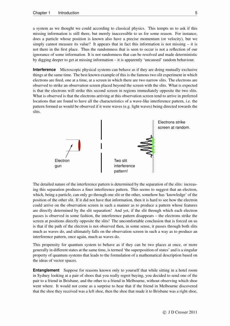
Interference Microscopic physical systems can behave as if they are doing mutually exclusivethings at the same time. The best known example of this is the famous two slit experiment in whichelectrons are fired, one at a time, at a screen in which there are two narrow slits. The electrons areobserved to strike an observation screen placed beyond the screen with the slits. What is expectedis that the electrons will strike this second screen in regions immediately opposite the two slits.What is observed is that the electrons arriving at this observation screen tend to arrive in preferredlocations that are found to have all the characteristics of a wave-like interference pattern, i.e. thepattern formed as would be observed if it were waves (e.g. light waves) being directed towards theslits.
Two slitinterferencepattern!
Electrons strikescreen at random.
Electrongun
�����
The detailed nature of the interference pattern is determined by the separation of the slits: increas-ing this separation produces a finer interference pattern. This seems to suggest that an electron,which, being a particle, can only go through one slit or the other, somehow has ‘knowledge’ of theposition of the other slit. If it did not have that information, then it is hard to see how the electroncould arrive on the observation screen in such a manner as to produce a pattern whose featuresare directly determined by the slit separation! And yet, if the slit through which each electronpasses is observed in some fashion, the interference pattern disappears – the electrons strike thescreen at positions directly opposite the slits! The uncomfortable conclusion that is forced on usis that if the path of the electron is not observed then, in some sense, it passes through both slitsmuch as waves do, and ultimately falls on the observation screen in such a way as to produce aninterference pattern, once again, much as waves do.
This propensity for quantum system to behave as if they can be two places at once, or moregenerally in different states at the same time, is termed ‘the superposition of states’ and is a singularproperty of quantum systems that leads to the formulation of a mathematical description based onthe ideas of vector spaces.
Entanglement Suppose for reasons known only to yourself that while sitting in a hotel roomin Sydney looking at a pair of shoes that you really regret buying, you decided to send one of thepair to a friend in Brisbane, and the other to a friend in Melbourne, without observing which shoewent where. It would not come as a surprise to hear that if the friend in Melbourne discoveredthat the shoe they received was a left shoe, then the shoe that made it to Brisbane was a right shoe,
c© J D Cresser 2011

Chapter 1 Introduction 6
and vice versa. If this strange habit of splitting up perfectly good pairs of shoes and sending oneat random to Brisbane and the other to Melbourne were repeated many times, then while it is notpossible to predict for sure what the friend in, say Brisbane, will observe on receipt of a shoe, itis nevertheless always the case that the results observed in Brisbane and Melbourne were alwaysperfectly correlated – a left shoe paired off with a right shoe.
Similar experiments can be undertaken with atomic particles, though it is the spins of pairs ofparticles that are paired off: each is spinning in exactly the opposite fashion to the other, so that thetotal angular momentum is zero. Measurements are then made of the spin of each particle when itarrives in Brisbane, or in Melbourne. Here it is not so simple as measuring whether or not the spinsare equal and opposite, i.e. it goes beyond the simple example of left or right shoe, but the ideais nevertheless to measure the correlations between the spins of the particles. As was shown byJohn Bell, it is possible for the spinning particles to be prepared in states for which the correlationbetween these measured spin values is greater than what classical physics permits. The systemsare in an ‘entangled state’, a quantum state that has no classical analogue. This is a conclusionthat is experimentally testable via Bell’s inequalities, and has been overwhelmingly confirmed.Amongst other things it seems to suggest the two systems are ‘communicating’ instantaneously,i.e. faster than the speed of light which is inconsistent with Einstein’s theory of relativity. As itturns out, it can be shown that there is no faster-than-light communication at play here. But it canbe argued that this result forces us to the conclusion that physical systems acquire some (maybeall?) properties only through the act of observation, e.g. a particle does not ‘really’ have a specificposition until it is measured.
The sorts of quantum mechanical behaviour seen in the three instances discussed above are be-lieved to be common to all physical systems. So what is quantum mechanics? It is saying some-thing about all physical systems. Quantum mechanics is not a physical theory specific to a limitedrange of physical systems i.e. it is not a theory that applies only to atoms and molecules and thelike. It is a meta-theory. At its heart, quantum mechanics is a set of fundamental principles thatconstrain the form of physical theories themselves, whether it be a theory describing the mechan-ical properties of matter as given by Newton’s laws of motion, or describing the properties ofthe electromagnetic field, as contained in Maxwell’s equations or any other conceivable theory.Another example of a meta-theory is relativity — both special and general — which places strictconditions on the properties of space and time. In other words, space and time must be treated inall (fundamental) physical theories in a way that is consistent with the edicts of relativity.
To what aspect of all physical theories do the principles of quantum mechanics apply? The princi-ples must apply to theories as diverse as Newton’s Laws describing the mechanical properties ofmatter, Maxwell’s equations describing the electromagnetic field, the laws of thermodynamics –what is the common feature? The answer lies in noting how a theory in physics is formulated.
1.3 Observation, Information and the Theories of Physics
Modern physical theories are not arrived at by pure thought (except, maybe, general relativity).The common feature of all physical theories is that they deal with the information that we can ob-tain about physical systems through experiment, or observation. For instance, Maxwell’s equationsfor the electromagnetic field are little more than a succinct summary of the observed properties ofelectric and magnetic fields and any associated charges and currents. These equations were ab-stracted from the results of innumerable experiments performed over centuries, along with someclever interpolation on the part of Maxwell. Similar comments could be made about Newton’slaws of motion, or thermodynamics. Data is collected, either by casual observation or controlledexperiment on, for instance the motion of physical objects, or on the temperature, pressure, vol-ume of solids, liquids, or gases and so on. Within this data, regularities are observed which are
c© J D Cresser 2011

Chapter 1 Introduction 7
best summarized as equations:
F = ma — Newton’s second law;
∇ × E = −∂B∂t
— One of Maxwell’s equations (Faraday’s law);
PV = NkT — Ideal gas law (not really a fundamental law)
What these equations represent are relationships between information gained by observation ofvarious physical systems and as such are a succinct way of summarizing the relationship betweenthe data, or the information, collected about a physical system. The laws are expressed in a mannerconsistent with how we understand the world from the view point of classical physics in that thesymbols replace precisely known or knowable values of the physical quantities they represent.There is no uncertainty or randomness as a consequence of our ignorance of information about asystem implicit in any of these equations. Moreover, classical physics says that this information isa faithful representation of what is ‘really’ going on in the physical world. These might be calledthe ‘classical laws of information’ implicit in classical physics.
What these pre-quantum experimenters were not to know was that the information they weregathering was not refined enough to show that there were fundamental limitations to the accuracywith which they could measure physical properties. Moreover, there was some information thatthey might have taken for granted as being accessible, simply by trying hard enough, but which wenow know could not have been obtained at all! There was in operation unsuspected laws of naturethat placed constraints on the information that could be obtained about any physical system. Inthe absence in the data of any evidence of these laws of nature, the information that was gatheredwas ultimately organised into mathematical statements that constituted classical laws of physics:Maxwell’s equations, or Newton’s laws of motion. But in the late nineteenth century and oninto the twentieth century, experimental evidence began to accrue that suggested that there wassomething seriously amiss with the classical laws of physics: the data could no longer be fitted tothe equations, or, in other words, the theory could not explain the observed experimental results.The choice was clear: either modify the existing theories, or formulate new ones. It was the latterapproach that succeeded. Ultimately, what was formulated was a new set of laws of nature, thelaws of quantum mechanics, which were essentially a set of laws concerning the information thatcould be gained about the physical world.
These are not the same laws as implicit in classical physics. For instance, there are limits onthe information that can be gained about a physical system. For instance, if in an experiment wemeasure the position x of a particle with an accuracy1 of ∆x, and then measure the momentum pof the particle we find that the result for p randomly varies from one run of the experiment to thenext, spread over a range ∆p. But there is still law here. Quantum mechanics tells us that
∆x∆p ≥ 12~ — the Heisenberg Uncertainty Relation
Quantum mechanics also tells us how this information is processed e.g. as a system evolves intime (the Schrodinger equation) or what results might be obtained in in a randomly varying wayin a measurement. Quantum mechanics is a theory of information, quantum information theory.
What are the consequences? First, it seems that we lose the apparent certainty and determinismof classical physics, this being replaced by uncertainty and randomness. This randomness is notdue to our inadequacies as experimenters — it is built into the very fabric of the physical world.But on the positive side, these quantum laws mean that physical systems can do so much morewithin these restrictions. A particle with position or momentum uncertain by amounts ∆x and ∆pmeans we do not quite know where it is, or how fast it is going, and we can never know this. But
1Accuracy indicates closeness to the true value, precision is the repeatability or reproducibility of the measurement.
c© J D Cresser 2011

Chapter 1 Introduction 8
the particle can be doing a lot more things ‘behind the scenes’ as compared to a classical particleof precisely defined position and momentum. The result is infinitely richer physics — quantumphysics.
c© J D Cresser 2011

Chapter 2
The Early History of Quantum Mechanics
In the early years of the twentieth century, Max Planck, Albert Einstein, Louis de Broglie, NeilsBohr, Werner Heisenberg, Erwin Schrodinger, Max Born, Paul Dirac and others created the
theory now known as quantum mechanics. The theory was not developed in a strictly logical way– rather, a series of guesses inspired by profound physical insight and a thorough command of newmathematical methods was sewn together to create a theoretical edifice whose predictive poweris such that quantum mechanics is considered the most successful theoretical physics construct ofthe human mind. Roughly speaking the history is as follows:
Planck’s Black Body Theory (1900) One of the major challenges of theoretical physics towardsthe end of the nineteenth century was to derive an expression for the spectrum of the electromag-netic energy emitted by an object in thermal equilibrium at some temperature T . Such an object isknown as a black body, so named because it absorbs light of any frequency falling on it. A blackbody also emits electromagnetic radiation, this being known as black body radiation, and it was aformula for the spectrum of this radiation that was being sort for. One popular candidate for theformula was Wein’s law:
S( f ,T ) = α f 3e−β f /T (2.1)
f
S( f ,T )Rayleigh-Jeans
Planck
Wein
-
6
Figure 2.1: Rayleigh-Jeans (classical),Wein, and Planck spectral distributions.
The quantity S( f ,T ), otherwise known as the spec-tral distribution function, is such that S( f ,T )d f is theenergy contained in unit volume of electromagneticradiation in thermal equilibrium at an absolute tem-perature T due to waves of frequency between f andf + d f . The above expression for S was not so muchderived from a more fundamental theory as quite sim-ply guessed. It was a formula that worked well at highfrequencies, but was found to fail when improved ex-perimental techniques made it possible to measure Sat lower (infrared) frequencies. There was anothercandidate for S which was derived using argumentsfrom classical physics which lead to a formula forS( f ,T ) known as the Rayleigh-Jeans formula:
S( f ,T ) =8π f 2
c3 kBT (2.2)
where kB is a constant known as Boltzmann’s constant. This formula worked well at low fre-quencies, but suffered from a serious problem – it clearly increases without limit with increasingfrequency – there is more and more energy in the electromagnetic field at higher and higher fre-quencies. This amounts to saying that an object at any temperature would radiate an infinite
c© J D Cresser 2011

Chapter 2 The Early History of Quantum Mechanics 10
amount of energy at infinitely high frequencies. This result, ultimately to become known as the‘ultra-violet catastrophe’, is obviously incorrect, and indicates a deep flaw in classical physics.
In an attempt to understand the form of the spectrum of the electromagnetic radiation emittedby a black body, Planck proposed a formula which he obtained by looking for a formula thatfitted Wein’s law at high frequencies, and also fitted the new low frequency experimental results(which happen to be given by the Rayleigh-Jeans formula, though Planck was not aware of this).It was when he tried to provide a deeper explanation for the origin of this formula that he made animportant discovery whose significance even he did not fully appreciate.
In this derivation, Planck proposed that the atoms making up the black body object absorbed andemitted light of frequency f in multiples of a fundamental unit of energy, or quantum of energy,E = h f . On the basis of this assumption, he was able to rederive the formula he had earlierguessed:
S( f ,T ) =8πh f 3
c3
1exp(h f /kT ) − 1
. (2.3)
This curve did not diverge at high frequencies – there was no ultraviolet catastrophe. Moreover,by fitting this formula to experimental results, he was able to determine the value of the constanth, that is, h = 6.6218 × 10⁻³⁴Joule-sec. This constant was soon recognized as a new fundamentalconstant of nature, and is now known as Planck’s constant.
In later years, as quantum mechanics evolved, it was found that the ratio h/2π arose time andagain. As a consequence, Dirac introduced a new quantity ~ = h/2π, pronounced ‘h-bar’, whichis now the constant most commonly encountered. In terms of ~, Planck’s formula for the quantumof energy becomes
E = h f = (h/2π) 2π f = ~ω (2.4)
where ω is the angular frequency of the light wave.
Einstein’s Light Quanta (1905) Although Planck believed that the rule for the absorption andemission of light in quanta applied only to black body radiation, and was a property of the atoms,rather than the radiation, Einstein saw it as a property of electromagnetic radiation, whether it wasblack body radiation or of any other origin. In particular, in his work on the photoelectric effect,he proposed that light of frequency ω was made up of quanta or ‘packets’ of energy ~ω whichcould be only absorbed or emitted in their entirety.
Bohr’s Model of the Hydrogen Atom (1913) Bohr then made use of Einstein’s ideas in an at-tempt to understand why hydrogen atoms do not self destruct, as they should according to the lawsof classical electromagnetic theory. As implied by the Rutherford scattering experiments, a hydro-gen atom consists of a positively charged nucleus (a proton) around which circulates a very light(relative to the proton mass) negatively charged particle, an electron. Classical electromagnetismsays that as the electron is accelerating in its circular path, it should be radiating away energy inthe form of electromagnetic waves, and do so on a time scale of ∼ 10−12 seconds, during whichtime the electron would spiral into the proton and the hydrogen atom would cease to exist. Thisobviously does not occur.
Bohr’s solution was to propose that provided the electron circulates in orbits whose radii r satisfyan ad hoc rule, now known as a quantization condition, applied to the angular momentum L of theelectron
L = mvr = n~ (2.5)
where v is the speed of the electron and m its mass, and n a positive integer (now referred to asa quantum number), then these orbits would be stable – the hydrogen atom was said to be in astationary state. He could give no physical reason why this should be the case, but on the basis of
c© J D Cresser 2011

Chapter 2 The Early History of Quantum Mechanics 11
this proposal he was able to show that the hydrogen atom could only have energies given by theformula
En = −ke2
2a0
1n2 (2.6)
where k = 1/4πε0 and
a0 =4πε0~2
me2 = 0.0529 nm (2.7)
is known as the Bohr radius, and roughly speaking gives an indication of the size of an atom asdetermined by the rules of quantum mechanics. Later we shall see how an argument based on theuncertainty principle gives a similar result.
The tie-in with Einstein’s work came with the further proposal that the hydrogen atom emits orabsorbs light quanta by ‘jumping’ between the energy levels, such that the frequency f of thephoton emitted in a downward transition from the stationary state with quantum number ni toanother of lower energy with quantum number n f would be
f =Eni − En f
h=
ke2
2a0h
[1n2
f
−1n2
i
]. (2.8)
Einstein used these ideas of Bohr to rederive the black body spectrum result of Planck. In doingso, he set up the theory of emission and absorption of light quanta, including spontaneous (i.e.‘uncaused’ emission) – the first intimation that there were processes occurring at the atomic levelthat were intrinsically probabilistic. This work also lead him to the conclusion that the light quantawere more than packets of energy, but carried momentum in a particular direction – the light quantawere, in fact, particles, subsequently named photons by the chemist Gilbert Lewis.
There was some success in extracting a general method, now known as the ‘old’ quantum theory,from Bohr’s model of the hydrogen atom. But this theory, while quite successful for the hydrogenatom, was an utter failure when applied to even the next most complex atom, the helium atom.The ad hoc character of the assumptions on which it was based gave little clue to the nature of theunderlying physics, nor was it a theory that could describe a dynamical system, i.e. one that wasevolving in time. Its role seems to have been one of ‘breaking the ice’, freeing up the attitudes ofresearchers at that time to old paradigms, and opening up new ways of looking at the physics ofthe atomic world.
De Broglie’s Hypothesis (1924) Inspired by Einstein’s picture of light, a form of wave motion,as also behaving in some circumstances as if it was made up of particles, and inspired also bythe success of the Bohr model of the hydrogen atom, de Broglie was lead, by purely aestheticarguments to make a radical proposal: if light waves can behave under some circumstances likeparticles, then by symmetry it is reasonable to suppose that particles such as an electron (or aplanet?) can behave like waves. More precisely, if light waves of frequency ω can behave like acollection of particles of energy E = ~ω, then by symmetry, a massive particle of energy E, anelectron say, should behave under some circumstances like a wave of frequency ω = E/~. Butassigning a frequency to these waves is not the end of the story. A wave is also characterised by itswavelength, so it is also necessary to assign a wavelength to these ‘matter waves’. For a particleof light, a photon, the wavelength of the associated wave is λ = c/ f where f = ω/2π. So whatis it for a massive particle? A possible formula for this wavelength can be obtained by looking alittle further at the case of the photon. In Einstein’s theory of relativity, a photon is recognized asa particle of zero rest mass, and as such the energy of a photon (moving freely in empty space) isrelated to its momentum p by E = pc. From this it follows that
E = ~ω = ~ 2πc/λ = pc (2.9)
c© J D Cresser 2011

Chapter 2 The Early History of Quantum Mechanics 12
so that, since ~ = h/2πp = h/λ. (2.10)
This equation then gave the wavelength of the photon in terms of its momentum, but it is alsoan expression that contains nothing that is specific to a photon. So de Broglie assumed that thisrelationship applied to all free particles, whether they were photons or electrons or anything else,and so arrived at the pair of equations
f = E/h λ = h/p (2.11)
which gave the frequency and wavelength of the waves that were to be associated with a freeparticle of kinetic energy E and momentum p. Strictly speaking, the relativistic expressions forthe momentum and energy of a particle of non-zero rest mass ought to be used in these formula,as these above formulae were derived by making use of results of special relativity. However, herewe will be concerned solely with the non-relativistic limit, and so the non-relativistic expressions,E = 1
2 mv2 and p = mv will suffice1.
This work constituted de Broglie’s PhD thesis. It was a pretty thin affair, a few pages long, andwhile it was looked upon with some scepticism by the thesis examiners, the power and eleganceof his ideas and his results were immediately appreciated by Einstein, more reluctantly by others,and lead ultimately to the discovery of the wave equation by Schrodinger, and the development ofwave mechanics as a theory describing the atomic world.
Experimentally, the first evidence of the wave nature of massive particles was seen by Davissonand Germer in 1926 when they fired a beam of electrons of known energy at a nickel crystal inwhich the nickel atoms are arranged in a regular array. Much to the surprise of the experimenters(who were not looking for any evidence of wave properties of electrons), the electrons reflectedoff the surface of the crystal to form an interference pattern. The characteristics of this patternwere entirely consistent with the electrons behaving as waves, with a wavelength given by thede Broglie formula, that were reflected by the periodic array of atoms in the crystal (which actedmuch like slits in a diffraction grating).
r
λ
Figure 2.2: De Broglie wave for which fourwavelengths λ fit into a circle of radius r.
An immediate success of de Broglie’s hypothesis wasthat it gave an explanation, of sorts, of the quantizationcondition L = n~. If the electron circulating aroundthe nucleus is associated with a wave of wavelengthλ, then for the wave not to destructively interfere withitself, there must be a whole number of waves (seeFig. (2.2)) fitting into one circumference of the orbit,i.e.
nλ = 2πr. (2.12)
Using the de Broglie relation λ = h/p then gives L =
pr = n~ which is just Bohr’s quantization condition.But now, given that particles can exhibit wave likeproperties, the natural question that arises is: what isdoing the ‘waving’? Further, as wave motion is usually describable in terms of some kind ofwave equation, it is then also natural to ask what the wave equation is for these de Broglie waves.The latter question turned out to be much easier to answer than the first – these waves satisfy thefamous Schrodinger wave equation. But what these waves are is still, largely speaking, an incom-pletely answered question: are they ‘real’ waves, as Schrodinger believed, in the sense that theyrepresent some kind of physical vibration in the same way as water or sound or light waves, or are
1For a particle moving in the presence of a spatially varying potential, momentum is not constant so the wavelengthof the waves will also be spatially dependent – much like the way the wavelength of light waves varies as the wavemoves through a medium with a spatially dependent refractive index. In that case, the de Broglie recipe is insufficient,and a more general approach is needed – Schrodinger’s equation.
c© J D Cresser 2011

Chapter 2 The Early History of Quantum Mechanics 13
they something more abstract, waves carrying information, as Einstein seemed to be the first to in-timate. The latter is an interpretation that has been gaining in favour in recent times, a perspectivethat we can support somewhat by looking at what we can learn about a particle by studying theproperties of these waves. It is this topic to which we now turn.
c© J D Cresser 2011

Chapter 3
The Wave Function
On the basis of the assumption that the de Broglie relations give the frequency and wavelengthof some kind of wave to be associated with a particle, plus the assumption that it makes
sense to add together waves of different frequencies, it is possible to learn a considerable amountabout these waves without actually knowing beforehand what they represent. But studying differ-ent examples does provide some insight into what the ultimate interpretation is, the so-called Borninterpretation, which is that these waves are ‘probability waves’ in the sense that the amplitudesquared of the waves gives the probability of observing (or detecting, or finding – a number ofdifferent terms are used) the particle in some region in space. Hand-in-hand with this interpreta-tion is the Heisenberg uncertainty principle which, historically, preceded the formulation of theprobability interpretation. From this principle, it is possible to obtain a number of fundamentalresults even before the full machinery of wave mechanics is in place.
In this Chapter, some of the consequences of de Broglie’s hypothesis of associating waves withparticles are explored, leading to the concept of the wave function, and its probability interpreta-tion.
3.1 The Harmonic Wave Function
On the basis of de Broglie’s hypothesis, there is associated with a particle of energy E and mo-mentum p, a wave of frequency f and wavelength λ given by the de Broglie relations Eq. (2.11).It is more usual to work in terms of the angular frequency ω = 2π f and wave number k = 2π/λ sothat the de Broglie relations become
ω = E/~ k = p/~. (3.1)
With this in mind, and making use of what we already know about what the mathematical form isfor a wave, we are in a position to make a reasonable guess at a mathematical expression for thewave associated with the particle. The possibilities include (in one dimension)
Ψ(x, t) = A sin(kx − ωt), A cos(kx − ωt), Aei(kx−ωt), . . . (3.2)
At this stage, we have no idea what the quantity Ψ(x, t) represents physically. It is given the namethe wave function, and in this particular case we will use the term harmonic wave function todescribe any trigonometric wave function of the kind listed above. As we will see later, in generalit can take much more complicated forms than a simple single frequency wave, and is almostalways a complex valued function. In fact, it turns out that the third possibility listed above isthe appropriate wave function to associate with a free particle, but for the present we will workwith real wave functions, if only because it gives us the possibility of visualizing their form whilediscussing their properties.
c© J D Cresser 2011

Chapter 3 The Wave Function 15
In order to gain an understanding of what a wave function might represent, we will turn thingsaround briefly and look at what we can learn about a particle if we know what its wave function is.We are implicitly bypassing here any consideration of whether we can understand a wave functionas being a physical wave in the same way that a sound wave, a water wave, or a light wave arephysical waves, i.e. waves made of some kind of physical ‘stuff’. Instead, we are going to look ona wave function as something that gives us information on the particle it is associated with. To thisend, we will suppose that the particle has a wave function given by Ψ(x, t) = A cos(kx−ωt). Then,given that the wave has angular frequency ω and wave number k, it is straightforward to calculatethe wave velocity, that is, the phase velocity vp of the wave, which is just the velocity of the wavecrests. This phase velocity is given by
vp =ω
k=
~ω~k
=Ep
=
12 mv2
mv= 1
2 v. (3.3)
Thus, given the frequency and wave number of a wave function, we can determine the speed ofthe particle from the phase velocity of its wave function, v = 2vp. We could also try to learnfrom the wave function the position of the particle. However, the wave function above tells usnothing about where the particle is to be found in space. We can make this statement because thiswave function is more or less the same everywhere. For sure, the wave function is not exactly thesame everywhere, but any feature that we might decide as being an indicator of the position ofthe particle, say where the wave function is a maximum, or zero, will not do: the wave functionis periodic, so any feature, such as where the wave function vanishes, reoccurs an infinite numberof times, and there is no way to distinguish any one of these repetitions from any other, see Fig.(3.1).
Ψ(x, t)
x
Figure 3.1: A wave function of constant amplitude and wavelength. The wave is the same everywhere andso there is no distinguishing feature that could indicate one possible position of the particle from any other.
Thus, this particular wave function gives no information on the whereabouts of the particle withwhich it is associated. So from a harmonic wave function it is possible to learn how fast a particleis moving, but not what the position is of the particle.
3.2 Wave Packets
From what was said above, a wave function constant throughout all space cannot give informationon the position of the particle. This suggests that a wave function that did not have the sameamplitude throughout all space might be a candidate for a giving such information. In fact, sincewhat we mean by a particle is a physical object that is confined to a highly localized region inspace, ideally a point, it would be intuitively appealing to be able to devise a wave function thatis zero or nearly so everywhere in space except for one localized region. It is in fact possible toconstruct, from the harmonic wave functions, a wave function which has this property. To showhow this is done, we first consider what happens if we combine together two harmonic waveswhose wave numbers are very close together. The result is well-known: a ‘beat note’ is produced,i.e. periodically in space the waves add together in phase to produce a local maximum, while
c© J D Cresser 2011

Chapter 3 The Wave Function 16
midway in between the waves will be totally out of phase and hence will destructively interfere.This is illustrated in Fig. 3.2(a) where we have added together two waves cos(5x) + cos(5.25x).
(a)
(b)
(c)
(d)
Figure 3.2: (a) Beat notes produced by adding together two cos waves: cos(5x) + cos(5.25x).(b) Combining five cos waves: cos(4.75x) + cos(4.875x) + cos(5x) + cos(5.125x) + cos(5.25x).(c) Combining seven cos waves: cos(4.8125x) + cos(4.875x) + cos(4.9375x) + cos(5x) + cos(5.0625x) +
cos(5.125x) + cos(5.1875x).(d) An integral over a continuous range of wave numbers produces a single wave packet.
Now suppose we add five such waves together, as in Fig. 3.2(b). The result is that some beatsturn out to be much stronger than the others. If we repeat this process by adding seven wavestogether, but now make them closer in wave number, we get Fig. 3.2(c), we find that most of thebeat notes tend to become very small, with the strong beat notes occurring increasingly far apart.Mathematically, what we are doing here is taking a limit of a sum, and turning this sum into anintegral. In the limit, we find that there is only one beat note – in effect, all the other beat notesbecome infinitely far away. This single isolated beat note is usually referred to as a wave packet.
We need to look at this in a little more mathematical detail, so suppose we add together a largenumber of harmonic waves with wave numbers k1, k2, k3, . . . all lying in the range:
k − ∆k . kn . k + ∆k (3.4)
around a value k, i.e.
Ψ(x, t) =A(k1) cos(k1x − ω1t) + A(k2) cos(k2x − ω2t) + . . .
=∑
n
A(kn) cos(knx − ωnt) (3.5)
where A(k) is a function peaked about the value k with a full width at half maximum of 2∆k. (Thereis no significance to be attached to the use of cos functions here – the idea is simply to illustrate a
c© J D Cresser 2011

Chapter 3 The Wave Function 17
point. We could equally well have used a sin function or indeed a complex exponential.) What isfound is that in the limit in which the sum becomes an integral:
Ψ(x, t) =
∫ +∞
−∞
A(k) cos(kx − ωt) dk (3.6)
all the waves interfere constructively to produce only a single beat note as illustrated in Fig. 3.2(d)above1. The wave function or wave packet so constructed is found to have essentially zero ampli-tude everywhere except for a single localized region in space, over a region of width 2∆x, i.e. thewave function Ψ(x, t) in this case takes the form of a single wave packet, see Fig. (3.3).
1'-1"
8"
(a) (b)
2∆k
2∆x
xkk
Ψ(x, t)A(k)
Figure 3.3: (a) The distribution of wave numbers k of harmonic waves contributing to the wave functionΨ(x, t). This distribution is peaked about k with a width of 2∆k. (b) The wave packet Ψ(x, t) of width 2∆xresulting from the addition of the waves with distribution A(k). The oscillatory part of the wave packet (the‘carrier wave’) has wave number k.
This wave packet is clearly particle-like in that its region of significant magnitude is confined to alocalized region in space. Moreover, this wave packet is constructed out of a group of waves withan average wave number k, and so these waves could be associated in some sense with a particleof momentum p = ~k. If this were true, then the wave packet would be expected to move with avelocity of p/m. This is in fact found to be the case, as the following calculation shows.
Because a wave packet is made up of individual waves which themselves are moving, though notwith the same speed, the wave packet itself will move (and spread as well). The speed with whichthe wave packet moves is given by its group velocity vg:
vg =
(dωdk
)k=k. (3.7)
This is the speed of the maximum of the wave packet i.e. it is the speed of the point on the wavepacket where all the waves are in phase. Calculating the group velocity requires determining therelationship between ω to k, known as a dispersion relation. This dispersion relation is obtainedfrom
E = 12 mv2 =
p2
2m. (3.8)
1In Fig. 3.2(d), the wave packet is formed from the integral
Ψ(x, 0) =1
4√π
∫ +∞
−∞
e−((k−5)/4)2cos(kx) dk.
c© J D Cresser 2011

Chapter 3 The Wave Function 18
Substituting in the de Broglie relations Eq. (2.11) gives
~ω =~2k2
2m(3.9)
from which follows the dispersion relation
ω =~k2
2m. (3.10)
The group velocity of the wave packet is then
vg =
(dωdk
)k=k
=~km. (3.11)
Substituting p = ~k, this becomes vg = p/m. i.e. the packet is indeed moving with the velocityof a particle of momentum p, as suspected. This is a result of some significance, i.e. we haveconstructed a wave function of the form of a wave packet which is particle-like in nature. Butunfortunately this is done at a cost. We had to combine together harmonic wave functions cos(kx−ωt) with a range of k values 2∆k to produce a wave packet which has a spread in space of size2∆x. The two ranges of k and x are not unrelated – their connection is embodied in an importantresult known as the Heisenberg Uncertainty Relation.
3.3 The Heisenberg Uncertainty Relation
The wave packet constructed in the previous section obviously has properties that are reminiscentof a particle, but it is not entirely particle-like — the wave function is non-zero over a region inspace of size 2∆x. In the absence of any better way of relating the wave function to the positionof the atom, it is intuitively appealing to suppose that where Ψ(x, t) has its greatest amplitude iswhere the particle is most likely to be found, i.e. the particle is to be found somewhere in a regionof size 2∆x. More than that, however, we have seen that to construct this wavepacket, harmonicwaves having k values in the range (k − ∆k, k + ∆k) were adding together. These ranges ∆x and∆k are related by the bandwidth theorem, which applies when adding together harmonic waves,which tell us that
∆x∆k & 1. (3.12)
Using p = ~k, we have ∆p = ~∆k so that
∆x∆p & ~. (3.13)
A closer look at this result is warranted. A wave packet that has a significant amplitude withina region of size 2∆x was constructed from harmonic wave functions which represent a range ofmomenta p − ∆p to p + ∆p. We can say then say that the particle is likely to be found somewherein the region 2∆x, and given that wave functions representing a range of possible momenta wereused to form this wave packet, we could also say that the momentum of the particle will havea value in the range p − ∆p to p + ∆p2. The quantities ∆x and ∆p are known as uncertainties,and the relation above Eq. (3.14) is known as the Heisenberg uncertainty relation for position andmomentum.
All this is rather abstract. We do not actually ‘see’ a wave function accompanying its particle, sohow are we to know how ‘wide’ the wave packet is, and hence what the uncertainty in positionand momentum might be for a given particle, say an electron orbiting in an atomic nucleus, or the
2In fact, we can look on A(k) as a wave function for k or, since k = p/~ as effectively a wave function for momentumanalogous to Ψ(x, t) being a wave function for position.
c© J D Cresser 2011
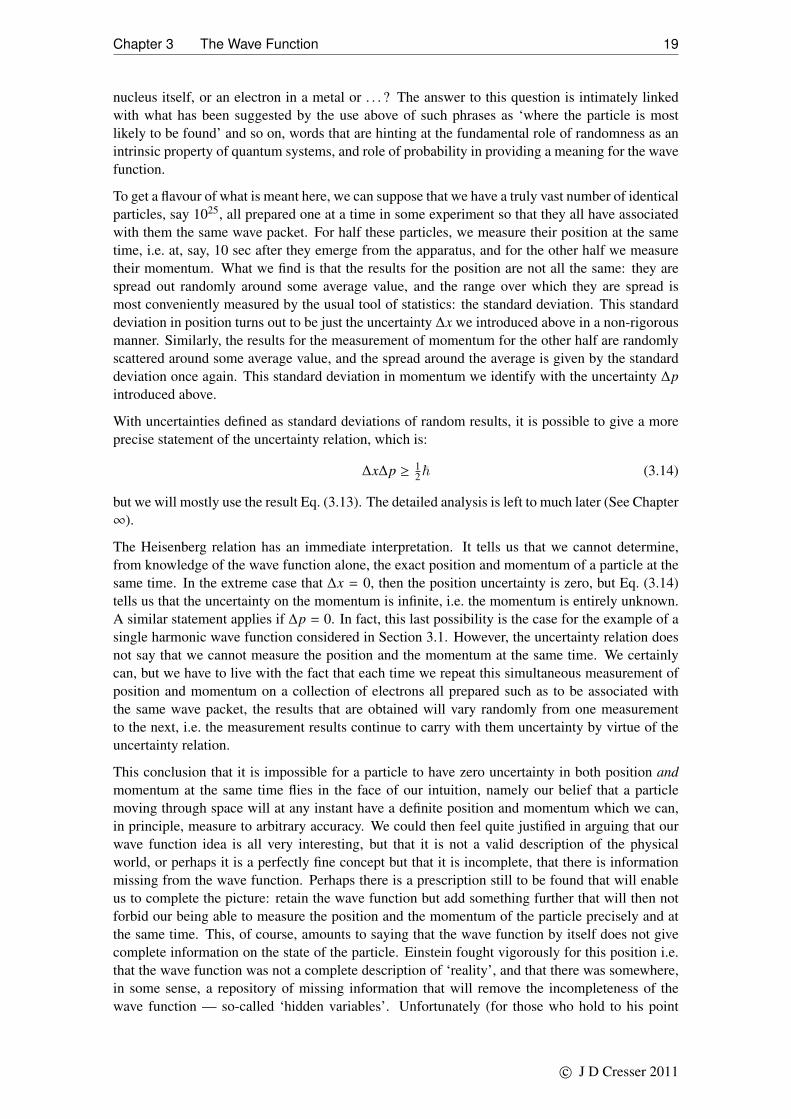
Chapter 3 The Wave Function 19
nucleus itself, or an electron in a metal or . . . ? The answer to this question is intimately linkedwith what has been suggested by the use above of such phrases as ‘where the particle is mostlikely to be found’ and so on, words that are hinting at the fundamental role of randomness as anintrinsic property of quantum systems, and role of probability in providing a meaning for the wavefunction.
To get a flavour of what is meant here, we can suppose that we have a truly vast number of identicalparticles, say 1025, all prepared one at a time in some experiment so that they all have associatedwith them the same wave packet. For half these particles, we measure their position at the sametime, i.e. at, say, 10 sec after they emerge from the apparatus, and for the other half we measuretheir momentum. What we find is that the results for the position are not all the same: they arespread out randomly around some average value, and the range over which they are spread ismost conveniently measured by the usual tool of statistics: the standard deviation. This standarddeviation in position turns out to be just the uncertainty ∆x we introduced above in a non-rigorousmanner. Similarly, the results for the measurement of momentum for the other half are randomlyscattered around some average value, and the spread around the average is given by the standarddeviation once again. This standard deviation in momentum we identify with the uncertainty ∆pintroduced above.
With uncertainties defined as standard deviations of random results, it is possible to give a moreprecise statement of the uncertainty relation, which is:
∆x∆p ≥ 12~ (3.14)
but we will mostly use the result Eq. (3.13). The detailed analysis is left to much later (See Chapter∞).
The Heisenberg relation has an immediate interpretation. It tells us that we cannot determine,from knowledge of the wave function alone, the exact position and momentum of a particle at thesame time. In the extreme case that ∆x = 0, then the position uncertainty is zero, but Eq. (3.14)tells us that the uncertainty on the momentum is infinite, i.e. the momentum is entirely unknown.A similar statement applies if ∆p = 0. In fact, this last possibility is the case for the example of asingle harmonic wave function considered in Section 3.1. However, the uncertainty relation doesnot say that we cannot measure the position and the momentum at the same time. We certainlycan, but we have to live with the fact that each time we repeat this simultaneous measurement ofposition and momentum on a collection of electrons all prepared such as to be associated withthe same wave packet, the results that are obtained will vary randomly from one measurementto the next, i.e. the measurement results continue to carry with them uncertainty by virtue of theuncertainty relation.
This conclusion that it is impossible for a particle to have zero uncertainty in both position andmomentum at the same time flies in the face of our intuition, namely our belief that a particlemoving through space will at any instant have a definite position and momentum which we can,in principle, measure to arbitrary accuracy. We could then feel quite justified in arguing that ourwave function idea is all very interesting, but that it is not a valid description of the physicalworld, or perhaps it is a perfectly fine concept but that it is incomplete, that there is informationmissing from the wave function. Perhaps there is a prescription still to be found that will enableus to complete the picture: retain the wave function but add something further that will then notforbid our being able to measure the position and the momentum of the particle precisely and atthe same time. This, of course, amounts to saying that the wave function by itself does not givecomplete information on the state of the particle. Einstein fought vigorously for this position i.e.that the wave function was not a complete description of ‘reality’, and that there was somewhere,in some sense, a repository of missing information that will remove the incompleteness of thewave function — so-called ‘hidden variables’. Unfortunately (for those who hold to his point
c© J D Cresser 2011

Chapter 3 The Wave Function 20
of view) evidence has mounted, particularly in the past few decades, that the wave function (orits analogues in the more general formulation of quantum mechanics) does indeed represent thefull picture — the most that can ever be known about a particle (or more generally any system)is what can be learned from its wave function. This means that the difficulty encountered aboveconcerning not being able to pinpoint the position and the momentum of a particle from knowledgeof its wave function is not a reflection of any inadequacy on the part of experimentalists trying tomeasure these quantities, but is an irreducible property of the natural world. Nevertheless, at themacroscopic level the uncertainties mentioned above become so small as to be experimentallyunmeasurable, so at this level the uncertainty relation has no apparent effect.
The limitations implied by the uncertainty relation as compared to classical physics may givethe impression that something has been lost, that nature has prevented us, to an extent quantifiedby the uncertainty principle, from having complete information about the physical world. Tosomeone wedded to the classical deterministic view of the the physical world (and Einstein wouldhave to be counted as one such person), it appears to be the case that there is information that ishidden from us. This may then be seen as a cause for concern because it implies that we cannot,even in principle, make exact predictions about the behaviour of any physical system. However,the view can be taken that the opposite is true, that the uncertainty principle is an indicator ofgreater freedom. In a sense, the uncertainty relation means it is possible for a physical system tohave a much broader range of possible physical properties consistent with the smaller amount ofinformation that is available about its properties. This leads to a greater richness in the propertiesof the physical world than could ever be found within classical physics.
3.3.1 The Heisenberg microscope: the effect of measurement
The Heisenberg Uncertainty Relation is enormously general. It applies without saying anythingwhatsoever about the nature of the particle, how it is prepared in an experiment, what it is doing,what it might be interacting with . . . . It is clearly a profoundly significant physical result. Butat its heart it is simply a mathematical statement about the properties of waves that flows fromthe assumed wave properties of matter plus some assumptions about the physical interpretationof these waves. There is little indication of what the physics might be that underlies it. One wayto uncover what physics might be present is to study what takes place if we attempt to measurethe position or the momentum of a particle. This is in fact the problem initially addressed byHeisenberg, and leads to a result that is superficially the same as 3.14, but, from a physics point ofview, there is in fact a subtle difference between what Heisenberg was doing, and what Eq. (3.14)is saying.
Heisenberg’s analysis was based on a thought experiment, i.e. an experiment that was not actuallyperformed, but was instead analysed as a mental construct. From this experiment, it is possibleto show, by taking account of the quantum nature of light and matter, that measuring the positionof an electron results in an unavoidable, unpredictable change in its momentum. More than that,it is possible to show that if the particle’s position were measured with ever increasing precision,the result was an ever greater disturbance of the particle’s momentum. This is an outcome that issummarized mathematically by a formula essentially the same as Eq. (3.14).
In his thought experiment, Heisenberg considered what was involved in attempting to measure theposition of a particle, an electron say, by shining light on the electron and observing the scatteredlight through a microscope. To analyse this measurement process, arguments are used which area curious mixture of ideas from classical optics (the wave theory of light) and from the quantumtheory of light (that light is made up of particles).
c© J D Cresser 2011

Chapter 3 The Wave Function 21
Figure 3.4: Airy disc diffraction patternproduced as image of a point object.
Classical optics enters the picture by virtue of the factthat in trying to measure the position of a point objectusing light, we must take into account the imprecisioninherent in such a measurement. If a point object is heldfixed (or is assumed to have infinite mass) and is illu-minated by a steady beam of light, then the image ofthis object, as produced by a lens on a photographic im-age plate, is not itself a point — it is a diffraction pat-tern, a smeared out blob, brightest in the centre of theblob and becoming darker towards the edges (forming aso-called Airy disc). If there are two closely positionedpoint objects, then what is observed is two overlappingdiffraction patterns. This overlap diminishes as the pointobjects are moved further apart until eventually, the edge of the central blob of one pattern willroughly coincide with the edge of the other blob, see Fig. (3.5).
Figure 3.5: Airy disc diffraction patternproduced as image of a pair of point ob-jects separated by distance d as give byEqn. (3.15).
The separation d between the point objects for whichthis occurs can be shown to be given by
d = 2λl
sinα(3.15)
where λl is the wavelength of the light, and 2α is the an-gle subtended at the lens by the object(s) (see Fig. (3.6)).This is a result that comes from the classical optics — itis essentially (apart from a factor of 2) the Rayleigh cri-terion for the resolution of a pair of images. For our pur-poses, we need to understand its meaning from a quan-tum mechanical perspective.
The quantum mechanical perspective arises because, ac-cording to quantum mechanics, a beam of light is to beviewed as a beam of individual particles, or photons. So,
if we have a steady beam of light illuminating the fixed point object as before, then what we willobserve on the photographic image plate is the formation of individual tiny spots, each associatedwith the arrival of a single photon. We would not see these individual photon arrivals with a nor-mal every-day light source: the onslaught of photon arrivals is so overwhelming that all we see isthe final familiar diffraction pattern. But these individual arrivals would be readily observed if thebeam of light is weak, i.e. there is plenty of time between the arrival of one photon and the next.This gives rise to the question: we have individual particles (photons) striking the photographicplate, so where does the diffraction pattern come from? Answering this question goes to the heartof quantum mechanics. If we were to monitor where each photon strikes the image plate over aperiod of time, we find that the photons strike at random, more often in the centre, helping to buildup the central bright region of the diffraction pattern, and more rarely towards the edges 3. Thisprobabilistic aspect of quantum mechanics we will study in depth in the following Chapter.
But what do we learn if we scatter just one photon off the point object? This photon will strikethe image plate at some point, but we will have no way of knowing for sure if the point where
3In fact, the formation of a diffraction pattern, from which comes the Rayleigh criterion Eq. (3.15) is itself a conse-quence of the ∆x∆p ≥ 1
2~ form of the uncertainty relation applied to the photon making its way through the lens. Theposition at which the photon passes through the lens can be specified by an uncertainty ∆x ≈ half the width of the lens,which means that the photon will acquire an uncertainty ∆p ≈ h/∆x in a direction parallel to the lens. This momentumuncertainty means that photons will strike the photographic plate randomly over a region whose size is roughly thewidth of the central maximum of the diffraction pattern.
c© J D Cresser 2011

Chapter 3 The Wave Function 22
the photon arrives is a point near the centre of the diffraction pattern, or near the edge of such apattern or somewhere in between — we cannot reconstruct the pattern from just one photon hit!But what we can say is that if one photon strikes the image plate, for example at the point c (onFig. 3.6), then this point could be anywhere between two extreme possibilities. We could arguethat the point object was sitting at a, and the photon has scattered to the far right of the diffractionpattern that would be built up by many photons being scattered from a point object at positiona (labelled A in Fig. 3.6), or we could argue at the other extreme that the point object was at b,and the photon reaching c has simply landed at the far left hand edge of the diffraction pattern(labelled B in Fig. 3.6) associated with a point particle sitting at b. Or the point object could besomewhere in between a and b, in which case c would be within the central maximum of theassociated diffraction pattern. The whole point is that the arrival of the photon at c is not enoughfor us to specify with certainty where the point object was positioned when it scattered the photon.If we let 2δx be the separation between a and b, then the best we can say, after detecting onephoton only, is that the point object that scattered it was somewhere in the region between a andb, i.e., we can specify the position of the point object only to an accuracy of ±δx. The argumentthat leads to Eq. (3.15) applies here, so we must put d = 2δx in Eq. (3.15) and hence we have
δx =λl
sinα. (3.16)
Note that the δx introduced here is to be understood as the resolution of the microscope. It is aproperty of the apparatus that we are using to measure the position of the fixed point object andso is not the same as the uncertainty ∆x introduced earlier that appears in Eq. (3.14), that being aproperty of the wave function of the particle.
••
•
α
A B
Lens
a b
c
electron in here‘somewhere’.
Figure 3.6: Diffraction images A and B cor-responding to two extreme possible positionsof a point object scattering a single photonthat arrives at c. If one photon strikes the im-age plate, the point c where it arrives could beanywhere between two extreme possibilities:on the extreme right of the cenral maximumof a diffraction pattern (labelled A) built upby many photons scattered from a point ob-ject at position a, or on the extreme left ofsuch a pattern (labelled B) built up by manyphotons being scattered from a point object atposition b. With 2δx the separation beween aand b, the best we can say, after detecting onephoton only, is that the object that scattered itwas somewhere in the region between a andb, i.e., we can specify the position of the ob-ject only to an accuracy of ±δx.
Now we turn to the experiment of interest, namely that of measuring the position of an electronpresumably placed in the viewing range of the observing lens arrangement. In measuring itsposition we want to make sure that we disturb its position as little as possible. We can do thisby using light whose intensity is as low as possible. Classically, this is not an issue: we can‘turn down’ the light intensity to be as small as we like. But quantum mechanics gets in the wayhere. Given the quantum nature of light, the minimum intensity possible is that associated with theelectron scattering only one photon. As we saw above, this single scattering event will enable us to
c© J D Cresser 2011
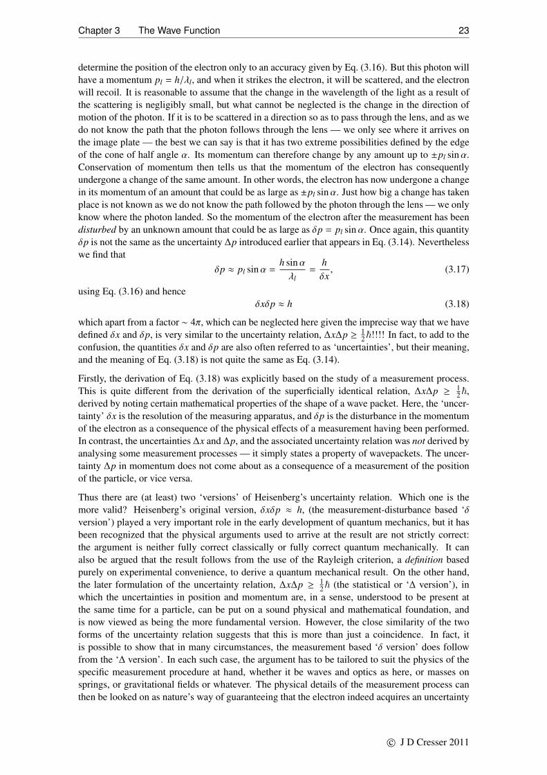
Chapter 3 The Wave Function 23
determine the position of the electron only to an accuracy given by Eq. (3.16). But this photon willhave a momentum pl = h/λl, and when it strikes the electron, it will be scattered, and the electronwill recoil. It is reasonable to assume that the change in the wavelength of the light as a result ofthe scattering is negligibly small, but what cannot be neglected is the change in the direction ofmotion of the photon. If it is to be scattered in a direction so as to pass through the lens, and as wedo not know the path that the photon follows through the lens — we only see where it arrives onthe image plate — the best we can say is that it has two extreme possibilities defined by the edgeof the cone of half angle α. Its momentum can therefore change by any amount up to ±pl sinα.Conservation of momentum then tells us that the momentum of the electron has consequentlyundergone a change of the same amount. In other words, the electron has now undergone a changein its momentum of an amount that could be as large as ±pl sinα. Just how big a change has takenplace is not known as we do not know the path followed by the photon through the lens — we onlyknow where the photon landed. So the momentum of the electron after the measurement has beendisturbed by an unknown amount that could be as large as δp = pl sinα. Once again, this quantityδp is not the same as the uncertainty ∆p introduced earlier that appears in Eq. (3.14). Neverthelesswe find that
δp ≈ pl sinα =h sinαλl
=hδx, (3.17)
using Eq. (3.16) and henceδxδp ≈ h (3.18)
which apart from a factor ∼ 4π, which can be neglected here given the imprecise way that we havedefined δx and δp, is very similar to the uncertainty relation, ∆x∆p ≥ 1
2~!!!! In fact, to add to theconfusion, the quantities δx and δp are also often referred to as ‘uncertainties’, but their meaning,and the meaning of Eq. (3.18) is not quite the same as Eq. (3.14).
Firstly, the derivation of Eq. (3.18) was explicitly based on the study of a measurement process.This is quite different from the derivation of the superficially identical relation, ∆x∆p ≥ 1
2~,derived by noting certain mathematical properties of the shape of a wave packet. Here, the ‘uncer-tainty’ δx is the resolution of the measuring apparatus, and δp is the disturbance in the momentumof the electron as a consequence of the physical effects of a measurement having been performed.In contrast, the uncertainties ∆x and ∆p, and the associated uncertainty relation was not derived byanalysing some measurement processes — it simply states a property of wavepackets. The uncer-tainty ∆p in momentum does not come about as a consequence of a measurement of the positionof the particle, or vice versa.
Thus there are (at least) two ‘versions’ of Heisenberg’s uncertainty relation. Which one is themore valid? Heisenberg’s original version, δxδp ≈ h, (the measurement-disturbance based ‘δversion’) played a very important role in the early development of quantum mechanics, but it hasbeen recognized that the physical arguments used to arrive at the result are not strictly correct:the argument is neither fully correct classically or fully correct quantum mechanically. It canalso be argued that the result follows from the use of the Rayleigh criterion, a definition basedpurely on experimental convenience, to derive a quantum mechanical result. On the other hand,the later formulation of the uncertainty relation, ∆x∆p ≥ 1
2~ (the statistical or ‘∆ version’), inwhich the uncertainties in position and momentum are, in a sense, understood to be present atthe same time for a particle, can be put on a sound physical and mathematical foundation, andis now viewed as being the more fundamental version. However, the close similarity of the twoforms of the uncertainty relation suggests that this is more than just a coincidence. In fact, itis possible to show that in many circumstances, the measurement based ‘δ version’ does followfrom the ‘∆ version’. In each such case, the argument has to be tailored to suit the physics of thespecific measurement procedure at hand, whether it be waves and optics as here, or masses onsprings, or gravitational fields or whatever. The physical details of the measurement process canthen be looked on as nature’s way of guaranteeing that the electron indeed acquires an uncertainty
c© J D Cresser 2011

Chapter 3 The Wave Function 24
δp ≈ h/δx in its momentum if its position is measured with an uncertainty δx, while lurking inthe background is the ‘∆ version’ of the uncertainty relation: in the example considered here, thisdescribes how the uncertainty in the path followed by the photon through the lens leads to theformation of the diffraction pattern (see footnote 3 on p21). But the correspondence is not perfect— the two versions are not completely equivalent. No one has ever been able to show that Eq.(3.18) always follows from Eq. (3.14) for all and any measurement procedure, and for good reason.Einstein, Podolsky and Rosen showed that here are methods by which the position of a particlecan be measured without physically interacting with the particle at all, so there is no prospect ofthe measurement disturbing the position of the particle.
Heisenberg’s uncertainty principle has always been a source of both confusion and insight, nothelped by Heisenberg’s own shifting interpretation of his own work, and is still a topic that attractssignificant research. The measurement-based ‘δ version’ has physical appeal as it seems to capturein an easily grasped fashion some of the peculiar predictions of quantum mechanics: measure theposition of a particle to great accuracy, for instance, and you unavoidably thoroughly screw upits momentum. That performing an observation on a physical system can affect the system in anuncontrollably random fashion has been termed the ‘observer effect’, and is an aspect of quantummechanics that has moved outside the purvey solely of quantum theory into other fields (such associology, for instance) involving the effects of making observations on other systems. But thestatistical ‘∆ version’ is wholly quantum mechanical, and represents a significant constraint on theway physical systems can behave, and has remarkable predictive powers that belies the simplicityof its statement, as we will see in the next section.
3.3.2 The Size of an Atom
One important application of the uncertainty relation is to do with determining the size of atoms.Recall that classically atoms should not exist: the electrons must spiral into the nucleus, radiatingaway their excess energy as they do. However, if this were the case, then the situation would bearrived at in which the position and the momentum of the electrons would be known: stationary,and at the position of the nucleus. This is in conflict with the uncertainty principle, so it must bethe case that the electron can spiral inward no further than an amount that is consistent with theuncertainty principle.
To see what the uncertainty principle does tell us about the behaviour of the electrons in an atom,consider as the simplest example a hydrogen atom. Here the electron is trapped in the Coulombpotential well due to the positive nucleus. We can then argue that if the electron cannot havea precisely defined position, then we can at least suppose that it is confined to a spherical (bysymmetry) shell of radius a. Thus, the uncertainty ∆x in x will be a, and similarly for the y andz positions. But, with the electron moving within this region, the x component of momentum,px, will, also by symmetry, swing between two equal and opposite values, p and −p say, andhence px will have an uncertainty of ∆px ≈ p. By appealing to symmetry once again, the y and zcomponents of momentum can be seen to have the same uncertainty.
By the uncertainty principle ∆px∆x ≈ ~, (and similarly for the other two components), the uncer-tainty in the x component of momentum will then be ∆px ≈ ~/a, and hence p ≈ ~/a. The kineticenergy of the particle will then be
T =p2
2m≈
~2
2ma2 (3.19)
so including the Coulomb potential energy, the total energy of the particle will be
E ≈~2
2ma2 −e2
4πε0a. (3.20)
c© J D Cresser 2011

Chapter 3 The Wave Function 25
The lowest possible energy of the atom is then obtained by simple differential calculus. Thus,taking the derivative of E with respect to a and equating this to zero and solving for a gives
a ≈4πε0~2
me2 ≈ 0.5 nm (3.21)
and the minimum energy
Emin ≈ −12
me4
(4πε0)2~2 (3.22)
≈ − 13.6 eV. (3.23)
The above values for atomic size and atomic energies are what are observed in practice. Theuncertainty relation has yielded considerable information on atomic structure without knowingall that much about what a wave function is supposed to represent! The exactness of the aboveresult is somewhat fortuitous, but the principle is nevertheless correct: the uncertainty principledemands that there be a minimum size to an atom. If a hydrogen atom has an energy above thisminimum, it is free to radiate away energy by emission of electromagnetic energy (light) untilit reaches this minimum. Beyond that, it cannot radiate any more energy. Classical EM theorysays that it should, but it does not. The conclusion is that there must also be something amisswith classical EM theory, which in fact turns out to be the case: the EM field too must treatedquantum mechanically. When this is done, there is consistency between the demands of quantumEM theory and the quantum structure of atoms – an atom in its lowest energy level (the groundstate) cannot, in fact, radiate – the ground state of an atom is stable.
Another important situation for which the uncertainty principle gives a surprising amount of in-formation is that of the harmonic oscillator.
3.3.3 The Minimum Energy of a Simple Harmonic Oscillator
By using Heisenberg’s uncertainty principle in the form ∆x∆p ≈ ~, it is also possible to esti-mate the lowest possible energy level (ground state) of a simple harmonic oscillator. The simpleharmonic oscillator potential is given by
U = 12 mω2x2 (3.24)
where m is the mass of the oscillator and ω is its natural frequency of oscillation. This is aparticularly important example as the simple harmonic oscillator potential is found to arise ina wide variety of circumstances such as an electron trapped in a well between two nuclei, or theoscillations of a linear molecule, or indeed in a manner far removed from the image of an oscillatoras a mechanical object, the lowest energy of a single mode quantum mechanical electromagneticfield.
We start by assuming that in the lowest energy level, the oscillations of the particle have an ampli-tude of a, so that the oscillations swing between −a and a. We further assume that the momentumof the particle can vary between p and −p. Consequently, we can assign an uncertainty ∆x = ain the position of the particle, and an uncertainty ∆p = p in the momentum of the particle. Thesetwo uncertainties will be related by the uncertainty relation
∆x∆p ≈ ~ (3.25)
from which we conclude thatp ≈ ~/a. (3.26)
c© J D Cresser 2011

Chapter 3 The Wave Function 26
The total energy of the oscillator is
E =p2
2m+ 1
2 mω2x2 (3.27)
so that roughly, if a is the amplitude of the oscillation, and p ≈ ~/a is the maximum momentumof the particle then
E ≈ 12
(1
2m~2
a2 + 12 mω2a2
)(3.28)
where the extra factor of 12 is included to take account of the fact that the kinetic and potential
energy terms are each their maximum possible values.
The minimum value of E can be found using differential calculus i.e.
dEda
= 12
(−
1m~2
a3 + mω2a)
= 0. (3.29)
Solving for a gives
a2 =~
mω. (3.30)
Substituting this into the expression for E then gives for the minimum energy
Emin ≈12~ω. (3.31)
A more precise quantum mechanical calculation shows that this result is (fortuitously) exactlycorrect, i.e. the ground state of the harmonic oscillator has a non-zero energy of 1
2~ω.
It was Heisenberg’s discovery of the uncertainty relation, and various other real and imaginedexperiments that ultimately lead to a fundamental proposal (by Max Born) concerning the physicalmeaning of the wave function. We shall arrive at this interpretation by way of the famous two slitinterference experiment.
c© J D Cresser 2011

Chapter 4
The Two Slit Experiment
This experiment is said to illustrate the essential mystery of quantum mechanics1. This mysteryis embodied in the apparent ability of a system to exhibit properties which, from a classical
physics point-of-view, are mutually contradictory. We have already touched on one such instance,in which the same physical system can exhibit under different circumstances, either particle orwave-like properties, otherwise known as wave-particle duality. This property of physical systems,otherwise known as ‘the superposition of states’, must be mirrored in a mathematical language interms of which the behaviour of such systems can be described and in some sense ‘understood’.As we shall see in later chapters, the two slit experiment is a means by which we arrive at this newmathematical language.
The experiment will be considered in three forms: performed with macroscopic particles, withwaves, and with electrons. The first two experiments merely show what we expect to see basedon our everyday experience. It is the third which displays the counterintuitive behaviour of mi-croscopic systems – a peculiar combination of particle and wave like behaviour which cannot beunderstood in terms of the concepts of classical physics. The analysis of the two slit experimentpresented below is more or less taken from Volume III of the Feynman Lectures in Physics.
4.1 An Experiment with Bullets
Imagine an experimental setup in which a machine gun is spraying bullets at a screen in whichthere are two narrow openings, or slits which may or may not be covered. Bullets that pass throughthe openings will then strike a further screen, the detection or observation screen, behind the first,and the point of impact of the bullets on this screen are noted.
Suppose, in the first instance, that this experiment is carried out with only one slit opened, slit 1say. A first point to note is that the bullets arrive in ‘lumps’, (assuming indestructible bullets),i.e. every bullet that leaves the gun (and makes it through the slits) arrives as a whole somewhereon the detection screen. Not surprisingly, what would be observed is the tendency for the bulletsto strike the screen in a region somewhere immediately opposite the position of the open slit, butbecause the machine gun is firing erratically, we would expect that not all the bullets would strikethe screen in exactly the same spot, but to strike the screen at random, though always in a regionroughly opposite the opened slit. We can represent this experimental outcome by a curve P1(x)which is simply such that
P1(x) δx = probability of a bullet landing in the range (x, x + δx). (4.1)
1Another property of quantum systems, known as ‘entanglement’, sometimes vies for this honour, but entanglementrelies on this ‘essential mystery’ we are considering here
c© J D Cresser 2011

Chapter 4 The Two Slit Experiment 28
If we were to cover this slit and open the other, then what we would observe is the tendency forthe bullets to strike the screen opposite this opened slit, producing a curve P2(x) similar to P1(x).These results are indicated in Fig. (4.1).
(a) (b)
P1(x)
P2(x)
Figure 4.1: The result of firing bullets at the screen when only one slit is open. The curves P1(x) and P2(x)give the probability densities of a bullet passing through slit 1 or 2 respectively and striking the screen at x.
Finally, suppose that both slits are opened. We would then observe the bullets would sometimescome through slit 1 and sometimes through slit 2 – varying between the two possibilities in arandom way – producing two piles behind each slit in a way that is simply the sum of the resultsthat would be observed with one or the other slit opened, i.e.
P12(x) = P1(x) + P2(x) (4.2)
Figure 4.2: The result of firing bulletsat the screen when both slits are open.The bullets accumulate on an observationscreen, forming two small piles oppositeeach slit. The curve P12(x) represents theprobability density of bullets landing atpoint x on the observation screen.
Slit 1
Slit 2
Observation screen
P12(x)
In order to quantify this last statement, we construct a histogram with which to specify the waythe bullets spread themselves across the observation screen. We start by assuming that this screenis divided up into boxes of width δx, and then count the number of bullets that land in each box.Suppose that the number of bullets fired from the gun is N, where N is a large number. If δN(x)bullets land in the box occupying the range x to x + δx then we can plot a histogram of δN/Nδx,the fraction of all the bullets that arrive, per unit length, in each interval over the entire width ofthe screen.
If the number of bullets is very large, and the width δx sufficiently small, then the histogram willdefine a smooth curve, P(x) say. What this quantity P(x) represents can be gained by considering
P(x) δx =δNN
(4.3)
which is the fraction of all the bullets fired from the gun that end up landing on the screen in regionx to x + δx. In other words, if N is very large, P(x) δx approximates to the probability that anygiven bullet will arrive at the detection screen in the range x to x + δx. An illustrative example is
c© J D Cresser 2011

Chapter 4 The Two Slit Experiment 29
given in Fig. (4.3) of the histogram obtained when 133 bullets strike the observation screen whenboth slits are open. In this figure the approximate curve for P(x) also plotted, which in this casewill be P12(x).
P(x) =δNNδx
x
δx
δN(x)
112361113129667101312106311
(a) (b)
Figure 4.3: Bullets that have passed through the first screen collected in boxes all of the same size δx. (a)The number of bullets that land in each box is presented. There are δN(x) bullets in the box between x andx + δx. (b) A histogram is formed from the ratio P(x) ≈ δN/Nδx where N is the total number of bulletsfired at the slits.
We can do the same in the two cases in which one or the other of the two slits are open. Thus, ifslit 1 is open, then we get the curve P1(x) in Fig. (4.2(a)), while if only slit 2 is open, we get P2(x)such as that in Fig. (4.2(b)). What we are then saying is that if we leave both slits open, then theresult will be just the sum of the two single slit curves, i.e.
P12(x) = P1(x) + P2(x). (4.4)
In other words, the probability of a bullet striking the screen in some region x to x + δx whenboth slits are opened is just the sum of the probabilities of the bullet landing in region when oneslit and then the other is closed. This is all perfectly consistent with what we understand aboutthe properties and behaviour of macroscopic objects — they arrive in indestructible lumps, andthe probability observed with two slits open is just the sum of the probabilities with each openindividually.
4.2 An Experiment with Waves
Now repeat the experiment with waves. For definiteness, let us suppose that the waves are lightwaves of wavelength λ. The waves pass through the slits and then impinge on the screen wherewe measure the intensity of the waves as a function of position along the screen.
c© J D Cresser 2011

Chapter 4 The Two Slit Experiment 30
First perform this experiment with one of the slits open, the other closed. The resultant intensitydistribution is then a curve which peaks behind the position of the open slit, much like the curveobtained in the experiment using bullets. Call it I1(x), which we know is just the square of theamplitude of the wave incident at x which originated from slit 1. If we deal only with the electricfield, and let the amplitude2 of the wave at x at time t be E(x, t) = E(x) exp(−iωt) in complexnotation, then the intensity of the wave at x will be
I1(x) = |E1(x, t)|2 = E1(x)2. (4.5)
Close this slit and open the other. Again we get a curve which peaks behind the position of theopen slit. Call it I2(x). These two outcomes are illustrated in Fig. (4.4).
(a) (b)
I1(x)
I2(x)
Figure 4.4: The result of directing waves at a screen when only one slit is open. The curves I1(x) and I2(x)give the intensities of the waves passing through slit 1 or 2 respectively and reaching the screen at x. (Theyare just the central peak of a single slit diffraction pattern.)
Now open both slits. What results is a curve on the screen I12(x) which oscillates between maximaand minima – an interference pattern, as illustrated in Fig. (4.5). In fact, the theory of interferenceof waves tells us that
I12(x) =|E1(x, t) + E2(x, t)|2
=I1(x) + I2(x) + 2E1E2 cos(2πd sin θ/λ
)=I1(x) + I2(x) + 2
√I1(x)I2(x) cos δ (4.6)
I12(x)
Figure 4.5: The usual two slit interference pattern.
where δ = 2πd sin θ/λ is the phase differencebetween the waves from the two slits arrivingat point x on the screen at an angle θ to thestraight through direction. This is certainlyquite different from what was obtained withbullets where there was no interference term.Moreover, the detector does not register the ar-rival of individual lumps of wave energy: thewaves arrive everywhere at the same time, andthe intensity can have any value at all.
2The word ‘amplitude’ is used here to represent the value of the wave at some point in time and space, and is notused to represent the maximum value of an oscillating wave.
c© J D Cresser 2011

Chapter 4 The Two Slit Experiment 31
4.3 An Experiment with Electrons
We now repeat the experiment for a third time, but in this case we use electrons. Here we imaginethat there is a beam of electrons incident normally on a screen with the two slits, with all the elec-trons having the same energy E and momentum p. The screen is a fluorescent screen, so that thearrival of each electron is registered as a flash of light – the signature of the arrival of a particle onthe screen. It might be worthwhile pointing out that the experiment to be described here was notactually performed until the very recent past, and even then not quite in the way described here.Nevertheless, the conclusions reached are what would be expected on the basis of what is nowknown about quantum mechanics from a multitude of other experiments. Thus, this largely hypo-thetical experiment (otherwise known as a thought experiment or gedanken experiment) serves toillustrate the kind of behaviour that quantum mechanics would produce, and in a way that can beused to establish the basic principles of the theory.
Let us suppose that the electron beam is made so weak that only one electron passes through theapparatus at a time. What we will observe on the screen will be individual point-flashes of light,and only one at a time as there is only one electron passing through the apparatus at a time. In otherwords, the electrons are arriving at the screen in the manner of particles, i.e. arriving in lumps. Ifwe close first slit 2 and observe the result we see a localization of flashes in a region directlyopposite slit 1. We can count up the number of flashes in a region of size δx to give the fractionof flashes that occur in the range x to x + δx, as in the case of the bullets. As there, we will callthe result P1(x). Now do the same with slit 1 closed and slit 2 opened. The result is a distributiondescribed by the curve P2(x). These two curves give, as in the case of the bullets, the probabilitiesof the electrons striking the screen when one or the other of the two slits are open. But, as in thecase of the bullets, this randomness is not to be seen as all that unexpected – the electrons makingtheir way from the source through the slits and then onto the screen would be expected to showevidence of some inconsistency in their behaviour which could be put down to, for instance, slightvariations in the energy and direction of propagation of each electron as it leaves the source.
Now open both slits. What we notice now is that these flashes do not always occur at the sameplace — in fact they appear to occur randomly across the screen. But there is a pattern to thisrandomness. If the experiment is allowed to continue for a sufficiently long period of time, whatis found is that there is an accumulation of flashes in some regions of the screen, and very few,or none, at other parts of the screen. Over a long enough observation time, the accumulation ofdetections, or flashes, forms an interference pattern, a characteristic of wave motion i.e. in contrastto what happens with bullets, we find that, for electrons, P12(x) , P1(x)+ P2(x). In fact, we obtaina result of the form
P12(x) = P1(x) + P2(x) + 2√
P1(x)P2(x) cos δ (4.7)
so we are forced to conclude that this is the result of the interference of two waves propagatingfrom each of the slits. One feature of the waves, namely their wavelength, can be immediatelydetermined from the separation between successive maxima of the interference pattern. It is foundthat δ = 2πd sin θ/λ where λ = h/p, and where p is the momentum of the incident electrons.Thus, these waves can be identified with the de Broglie waves introduced earlier, represented bythe wave function Ψ(x, t).
So what is going on here? If electrons are particles, like bullets, then it seems clear that theelectrons go either through slit 1 or through slit 2, because that is what particles would do. Thebehaviour of the electrons going through slit 1 should then not be affected by whether slit 2 isopened or closed as those electrons would go nowhere near slit 2. In other words, we have toexpect that P12(x) = P1(x) + P2(x), but this not what is observed. In fact, what is observed isimpossible to understand on the basis of this argument: if only one slit is open, say slit 1, then wefind electrons landing on the screen at points which, if we open slit 2, receive no electrons at all!
c© J D Cresser 2011
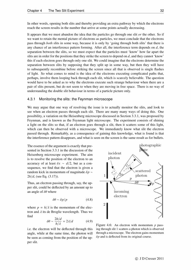
Chapter 4 The Two Slit Experiment 32
In other words, opening both slits and thereby providing an extra pathway by which the electronsreach the screen results in the number that arrive at some points actually decreasing.
It appears that we must abandon the idea that the particles go through one slit or the other. So ifwe want to retain the mental picture of electrons as particles, we must conclude that the electronspass through both slits in some way, because it is only by ‘going through both slits’ that there isany chance of an interference pattern forming. After all, the interference term depends on d, theseparation between the slits, so we must expect that the particles must ‘know’ how far apart theslits are in order for the positions that they strike the screen to depend on d, and they cannot ‘know’this if each electron goes through only one slit. We could imagine that the electrons determine theseparation between slits by supposing that they split up in some way, but then they will haveto subsequently recombine before striking the screen since all that is observed is single flashesof light. So what comes to mind is the idea of the electrons executing complicated paths that,perhaps, involve them looping back through each slit, which is scarcely believable. The questionwould have to be asked as to why the electrons execute such strange behaviour when there are apair of slits present, but do not seem to when they are moving in free space. There is no way ofunderstanding the double slit behaviour in terms of a particle picture only.
4.3.1 Monitoring the slits: the Feynman microscope
We may argue that one way of resolving the issue is to actually monitor the slits, and look tosee when an electron passes through each slit. There are many many ways of doing this. Onepossibility, a variation on the Heisenberg microscope discussed in Section 3.3.1, was proposed byFeynman, and is known as the Feynman light microscope. The experiment consists of shininga light on the slits so that, if an electron goes through a slit, then it scatters some of this light,which can then be observed with a microscope. We immediately know what slit the electronpassed through. Remarkably, as a consequence of gaining this knowledge, what is found is thatthe interference pattern disappears, and what is seen on the screen is the same result as for bullets.
1
2
incidentphoton
incomingelectron
scatteredphoton
photographicplate
p2α
δθ δp
Figure 4.6: An electron with momentum p pass-ing through slit 1 scatters a photon which is observedthrough a microscope. The electron gains momentumδp and is deflected from its original course.
The essence of the argument is exactly that pre-sented in Section 3.3.1 in the discussion of theHeisenberg microscope experiment. The aimis to resolve the position of the electron to anaccuracy of at least δx ∼ d/2, but as a con-sequence, we find that the electron is given arandom kick in momentum of magnitude δp ∼2h/d, (see Eq. (3.17)).
Thus, an electron passing through, say, the up-per slit, could be deflected by an amount up toan angle of δθ where
δθ ∼ δp/p (4.8)
where p = h/λ is the momentum of the elec-tron and λ its de Broglie wavelength. Thus wefind
δθ ∼2h/dh/λ
= 2λ/d (4.9)
i.e. the electron will be deflected through thisangle, while at the same time, the photon willbe seen as coming from the position of the up-per slit.
c© J D Cresser 2011

Chapter 4 The Two Slit Experiment 33
Since the angular separation between a maximum of the interference pattern and a neighbour-ing minimum is λ/2d, the uncertainty in the deflection of an observed electron is at least enoughto displace an electron from its path heading for a maximum of the interference pattern, to onewhere it will strike the screen at the position of a minimum. The overall result is to wipe out theinterference pattern.
But we could ask why it is that the photons could be scattered through a range of angles, i.e.why do we say ‘up to an angle of δθ’? After all, the experiment could be set up so that everyphoton sent towards the slits has the same momentum every time, and similarly for every electron,so every scattering event should produce the same result, and the outcome would merely be theinterference pattern displaced sideways. It is here where quantum randomness comes in. Theamount by which the electron is deflected depends on what angle the photon has been scatteredthrough, which amounts to knowing what part of the observation lens the photon goes through onits way to the photographic plate. But we cannot know this unless we ‘look’ to see where in thelens the photon passes. So there is an uncertainty in the position of the photon as it passes throughthe lens which, by the uncertainty relation, implies an uncertainty in the momentum of the photonin a direction parallel to the lens, so we cannot know with precision where the photon will landon the photographic plate. As a consequence, the position that each scattered photon will strikethe photographic plate will vary randomly from one scattered photon to the next in much the sameway as the position that the electron strikes the observation screen varies in a random fashion inthe original (unmonitored) two slit experiment. The uncertainty as to which slit the electron haspassed through has been transferred to the uncertainty about which part of the lens the scatteredphoton passes through.
So it would seem that by trying to determine through which slit the electron passes, the motionof the electron is always sufficiently disturbed so that no interference pattern is observed. As faras it is known, any experiment that can be devised – either a real experiment or a gedanken (i.e. athought) experiment – that involves directly observing through which slit the electrons pass alwaysresults in a disturbance in the motion of the electron sufficient for the interference pattern to bewiped out. An ‘explanation’ of why this occurs, of which the above discussion is an example,could perhaps be constructed in each case, but in any such explanation, the details of the waythe physics conspires to produce this result will differ from one experiment to the other 3. Theseexplanations often require a mixture of classical and quantum concepts, i.e. they have a foot inboth camps and as such are not entirely satisfactory, but more thorough studies of, for instance, theFeynman microscope experiment using a fully quantum mechanical approach, confirm the resultsdiscussed here. So it may come as a surprise to find that there need not be any direct physicalinteraction between the electrons and the apparatus used to monitor the slits, so there is no placefor the kind of quantum/classical explanation given above. It turns out that as long as there isinformation available regarding which slit the electron passes through, there is no interference, asthe following example illustrates.
4.3.2 The Role of Information: The Quantum Eraser
Suppose we construct the experimental set-up illustrated in Fig. (4.7). The actual experiment isperformed with photons, but we will stick with an ‘electron version’ here. In this experiment, theelectron source sends out pairs of particles. One of the pair (sometimes called the ‘signal’ particlein the photon version of the experiment) heads towards the slits, while the other (the ‘idler’) heads
3Einstein, who did not believe quantum mechanics was a complete theory, played the game of trying to find anexperimental setup that would bypass the uncertainty relation i.e. to know which slit an electron passes through AND toobserve an interference pattern. Bohr answered all of Einstein’s challenges, including, in one instance, using Einstein’sown theory of general relativity to defeat a proposal of Einstein’s concerning another form of the uncertainty relation,the time-energy uncertainty relation. It was at this point that Einstein abandoned the game, but not his attitude toquantum mechanics.
c© J D Cresser 2011

Chapter 4 The Two Slit Experiment 34
off at right angles. What we find here is that, if we send out many electrons in this fashion, thenno interference pattern is built up on the observation screen, i.e. we get the result we expect if weare able to determine through which slit each electron passes. But this outcome is not as puzzlingas it first might seem since, in fact, we actually do have this information: for each emitted electronthere is a correlated idler particle whose direction of motion will tell us in what direction theelectron is headed. Thus, in principle, we can determine which slit an electron will pass throughby choosing to detect the correlated idler particle by turning on detectors a and b. Thus, if wedetect a particle at a, then electron is heading for slit 1. However, we do not actually have to carryout this detection. The sheer fact that this information is available for us to access if we choose todo so is enough for the interference pattern not to appear.
1
2
Detector b
Detector a
These particlesare ‘carriers’ ofinformation
1
2
Single detectorerases ‘which path’information
Figure 4.7: Illustrating the ‘quantum eraser’ experiment.In the first set-up, the information on ‘which slit’ is en-coded in the auxiliary particle, and there is no interfer-ence. In the second, this information is erased and inter-ference is observed.
But suppose we wipe out this informationsomehow. If we make use of a single de-tector that is capable of detecting either ofthe idler particles, then we cannot tell, ifthis detector registers a count, which idlerparticle it detected. In this case, the ‘whichpath’ information has been erased. If weerase this information for every electron emit-ted, there will appear an interference pat-tern even though there has been no phys-ical interaction with the electrons passingthrough the slits!! This example suggeststhat provided there is information presentas to which slit an electron passes through,even if we do not access this information,then there is no interference pattern. This isan example of quantum entanglement: thedirection of the electron heading towardsthe slits is entangled with the direction ofthe ‘information carrier’ idler particle.
This more general analysis shows that thecommon feature in all these cases is thatthe electron becomes ‘entangled’ with some other system, in such a manner that this other systemcarries with it information about the electron. In this example, entanglement is present right fromthe start of the experiment, while in the monitoring-by-microscope example, entanglement withthe scattered photon has been actively established, with information on the position of the electronencoded in the photon. But that is all that we require, i.e. that the information be so encoded –we do not need to have some one consciously observe these photons for the interference patternto disappear, it is merely sufficient that this information be available. It is up to use to choose toaccess it or not.
What is learned from this is that if information is in principle available on the position of theelectron or, in other words, if we want to be anthropomorphic about all this, if we can in principleknow which slit the electron goes through by availing ourselves of this information, even withoutinterfering with the electron, then the observed pattern of the screen is the same as found withbullets: no interference, with P12(x) = P1(x) + P2(x). If this information is not available at all,then we are left with the uncomfortable thought that in some sense each electron passes throughboth slits, resulting in the formation of an interference pattern, the signature of wave motion. Thus,the electrons behave either like particles or like waves, depending on what information is extant, adichotomy that is known as wave-particle duality.
c© J D Cresser 2011

Chapter 4 The Two Slit Experiment 35
4.3.3 Wave-particle duality
So it appears that if we gain information on which slit the electron passes through then we losethe interference pattern. Gaining information on which slit means we are identifying the electronas a particle — only particles go through one slit or the other. But once this identification is made,say an electron has been identified as passing through slit 1, then that electron behaves thereafterlike a particle that has passed through one slit only, and so will contribute to the pattern normallyproduced when only slit 1 is open. And similarly for an electron identified as passing throughslit 2. Thus, overall, no interference pattern is produced. If we do not determined which slit, theelectrons behave as waves which are free to probe the presence of each slit, and so will give riseto an interference pattern.
This dichotomy, in which the same physical entity, an electron (or indeed, any particle), can bedetermined to be either a particle or a wave depending on what experiment is done to observe itsproperties, is known as wave-particle duality.
But in all instances, the inability to observe both the wave and particle properties – i.e. to knowwhich slit a particle passes through AND for there to be an interference pattern – can be tracedback to the essential role played by the uncertainty relation ∆x∆p ≥ 1
2~. As Feynman puts it, thisrelation ‘protects’ quantum mechanics. But note that this is NOT the measurement form of theuncertainty relation: there is no need for a disturbance to act on the particle as a consequence of ameasurement, for quantum mechanics to be protected, as we have just seen.
The fact that any situation for which there is information on which slit the electron passes throughalways results in the non-appearance of the interference pattern suggests that there is a deep phys-ical principle at play here – a law or laws of nature – that overrides, irrespective of the physicalset-up, any attempt to have information on where a particle is, and to observe interference effects.The laws are the laws of quantum mechanics, and one of their consequences is the uncertaintyprinciple, that is ∆x∆p ≥ 1
2~. If we want to pin down the slit through which the particle has pastwith, say, 97% certainty, then the consequent uncertainty ∆x in the position of the particle canbe estimated to be ∆x ≈ 0.17d, where d is the separation of the slits4. But doing so implies thatthere is an uncertainty in the sideways momentum of the electron given by ∆p & ~/0.17d. Thisamounts to a change in direction through an angle
∆θ =∆pp
&λ
2d(4.10)
Since the angular separation between a minimum and a neighbouring maximum of the diffractionpattern is λ/2d, it is clear that the uncertainty in the sideways momentum arising from trying toobserve through which slit the particle passes is enough to displace a particle from a maximuminto a neighbouring minimum, washing out the interference pattern.
Using the uncertainty principle in this way does not require us to invoke any ‘physical mechanism’to explain why the interference pattern washes out; only the abstract requirements of the uncer-tainty principle are used. Nothing is said about how the position of the particle is pinned down to
4This estimate is arrived at by recognizing that the measurement is not perfect, i.e. we cannot be totally sure, whena photon arrives on the photographic plate, which slit it came from. So, if we assign a probability P that the particle isat the slit with position d/2 and a probability 1 − P that it is at the position of the slit at −d/2 based on the observedoutcome of the measurement, then the mean position of the electron is now
〈x〉 = Pd/2 − (1 − P)d/2 = (P − 12 )d
and the standard deviation of this outcome is
(∆x)2 = P(d/2 − 〈x〉)2 + (1 − P)(−d/2 − 〈x〉)2 = P(1 − P)d
so ∆x =√
P(1 − P)d = 0.17d for P = 0.97.
c© J D Cresser 2011

Chapter 4 The Two Slit Experiment 36
within an uncertainty ∆x. If this information is provided, then a physical argument, of sorts, asin the case of Heisenberg’s microscope, that mixes classical and quantum mechanical ideas mightbe possible that explains why the interference pattern disappears. However, the details of the waythe physics conspires to produce this result will differ from one experiment to the other. And inany case, there might not be any physical interaction at all, as we have just seen. It is the laws ofquantum mechanics (from which the uncertainty principle follows) that tell us that the interferencepattern must disappear if we measure particle properties of the electrons, and this is so irrespectiveof the particular kind of physics involved in the measurement – the individual physical effects thatmay be present in one experiment or another are subservient to the laws of quantum mechanics.
4.4 Probability Amplitudes
First, a summary of what has been seen so far. In the case of waves, we have seen that the totalamplitude of the waves incident on the screen at the point x is given by
E(x, t) = E1(x, t) + E2(x, t) (4.11)
where E1(x, t) and E2(x, t) are the waves arriving at the point x from slits 1 and 2 respectively. Theintensity of the resultant interference pattern is then given by
I12(x) =|E(x, t)|2
=|E1(x, t) + E2(x, t)|2
=I1(x) + I2(x) + 2E1E2 cos(2πd sin θ
λ
)=I1(x) + I2(x) + 2
√I1(x)I2(x) cos δ (4.12)
where δ = 2πd sin θ/λ is the phase difference between the waves arriving at the point x from slits1 and 2 respectively, at an angle θ to the straight through direction. The point was then made thatthe probability density for an electron to arrive at the observation screen at point x had the sameform, i.e. it was given by the same mathematical expression
P12(x) = P1(x) + P2(x) + 2√
P1(x)P2(x) cos δ. (4.13)
so we were forced to conclude that this is the result of the interference of two waves propagatingfrom each of the slits. Moreover, the wavelength of these waves was found to be given by λ = h/p,where p is the momentum of the incident electrons so that these waves can be identified with the deBroglie waves introduced earlier, represented by the wave function Ψ(x, t). Thus, we are proposingthat incident on the observation screen is the de Broglie wave associated with each electron whosetotal amplitude at point x is given by
Ψ(x, t) = Ψ1(x, t) + Ψ2(x, t) (4.14)
where Ψ1(x, t) and Ψ2(x, t) are the amplitudes at x of the waves emanating from slits 1 and 2respectively. Further, since P12(x)δx is the probability of an electron being detected in the regionx, x + δx, we are proposing that
|Ψ(x, t)|2δx ∝ probability of observing an electron in x, x + δx (4.15)
so that we can interpret Ψ(x, t) as a probability amplitude. This is the famous probability inter-pretation of the wave function first proposed by Born on the basis of his own observations of theoutcomes of scattering experiments, as well as awareness of Einstein’s own inclinations alongthese lines. Somewhat later, after proposing his uncertainty relation, Heisenberg made a similarproposal.
There are two other important features of this result that are worth taking note of:
c© J D Cresser 2011

Chapter 4 The Two Slit Experiment 37
• If the detection event can arise in two different ways (i.e. electron detected after havingpassed through either slit 1 or 2) and the two possibilities remain unobserved, then the totalprobability of detection is
P = |Ψ1 + Ψ2|2 (4.16)
i.e. we add the amplitudes and then square the result.
• If the experiment contains a part that even in principle can yield information on which ofthe alternate paths were followed, then
P = P1 + P2 (4.17)
i.e. we add the probabilities associated with each path.
What this last point is saying, for example in the context of the two slit experiment, is that, as partof the experimental set-up, there is equipment that is monitoring through which slit the particlegoes. Even if this equipment is automated, and simply records the result, say in some computermemory, and we do not even bother to look the results, the fact that they are still available meansthat we should add the probabilities. This last point can be understood if we view the process ofobservation of which path as introducing randomness in such a manner that the interference effectsembodied in the cos δ are smeared out. In other words, the cos δ factor – which can range betweenplus and minus one – will average out to zero, leaving behind the sum of probability terms.
4.5 The Fundamental Nature of Quantum Probability
The fact that the results of the experiment performed with electrons yields outcomes which appearto vary in a random way from experiment to experiment at first appears to be identical to the sort ofrandomness that occurs in the experiment performed with the machine gun. In the latter case, therandom behaviour can be explained by the fact that the machine gun is not a very well constructeddevice: it sprays bullets all over the place. This seems to suggest that simply by refining theequipment, the randomness can be reduced, in principle removing it all together if we are cleverenough. At least, that is what classical physics would lead us to believe. Classical physics permitsunlimited accuracy in the fixing the values of physical or dynamical quantities, and our failure tolive up to this is simply a fault of inadequacies in our experimental technique.
However, the kind of randomness found in the case of the experiment performed with electronsis of a different kind. It is intrinsic to the physical system itself. We are unable to refine theexperiment in such a way that we can know precisely what is going on. Any attempt to do sogives rise to unpredictable changes, via the uncertainty principle. Put another way, it is foundthat experiments on atomic scale systems (and possibly at macroscopic scales as well) performedunder identical conditions, where everything is as precisely determined as possible, will always, ingeneral, yield results that vary in a random way from one run of the experiment to the next. Thisrandomness is irreducible, an intrinsic part of the physical nature of the universe.
Attempts to remove this randomness by proposing the existence of so-called ‘classical hiddenvariables’ have been made in the past. These variables are supposed to be classical in nature – weare simply unable to determine their values, or control them in any way, and hence give rise tothe apparent random behaviour of physical systems. Experiments have been performed that testthis idea, in which a certain inequality known as the Bell inequality, was tested. If these classicalhidden variables did in fact exist, then the inequality would be satisfied. A number of experimentshave yielded results that are clearly inconsistent with the inequality, so we are faced with havingto accept that the physics of the natural world is intrinsically random at a fundamental level, andin a way that is not explainable classically, and that physical theories can do no more than predictthe probabilities of the outcome of any measurement.
c© J D Cresser 2011

Chapter 5
Wave Mechanics
The version of quantum mechanics based on studying the properties of the wave function isknown as wave mechanics, and is the version that first found favour amongst early researchers
in the quantum theory, in part because it involved setting up and solving a partial differentialequation for the wave function, the famous Schrodinger equation, which was of a well-known andmuch studied form. As well as working in familiar mathematical territory, physicists and chemistswere also working with something concrete in what was in other ways a very abstract theory –the wave function was apparently a wave in space which could be visualized, at least to a certainextent. But it must be borne in mind that the wave function is not an objectively real entity, thewave function does not represent waves occurring in some material substance. Furthermore, itturns out that the wave function is no more than one aspect of a more general theory, quantumtheory, that is convenient for certain classes of problems, and entirely inappropriate (or indeedinapplicable) to others1. Nevertheless, wave mechanics offers a fairly direct route to some of themore important features of quantum mechanics, and for that reason, some attention is given hereto some aspects of wave mechanics prior to moving on, in later chapters, to considering the moregeneral theory.
5.1 The Probability Interpretation of the Wave Function
The probability interpretation of the wave function, due to Max Born, was introduced in the pre-ceding Chapter. It is restated here for convenience:
If a particle is described by a wave function Ψ(x, t), then
|Ψ(x, t)|2δx = Probability of observing the particle in the small region (x, x + δx) at time t
with the consequent terminology that the wave function is usually referred to as a ‘probabilityamplitude’.
What this interpretation means in a practical sense can be arrived at in a number of ways, theconventional manner making use of the notion of an ‘ensemble of identically prepared systems’.By this we mean that take a vast number of identical copies of the same system, in our case avery simple system, consisting on just one particle, and put them all through exactly the sameexperimental procedures, so that presumably they all end up in exactly the same physical state.An example would be the two slit experiment in which every electron is prepared with the samemomentum and energy. The collection of identical copies of the same system all prepared in the
1The wave function appears to be a wave in real space for a single particle, but that is only because it depends onx and t, in the same way as, say, the amplitude of a wave on a string can be written as a function of x and t. But, for asystem of more than one particle, the wave function becomes a function of two space variables x1 and x2 say, as well ast: Ψ(x1, x2, t). It then makes no sense to talk about the value of the wave function at some position in space. In fact, thewave function is a wave that ‘exists’ in an abstract space known as phase space.
c© J D Cresser 2011

Chapter 5 Wave Mechanics 39
same fashion is known as an ensemble. We then in effect assume that, at time t after the startof the preparation procedure, the state of each particle will be given by the same wave functionΨ(x, t), though it is common practice (and a point of contention) in quantum mechanics to say thatthe wave function describes the whole ensemble, not each one of its members. We will howeverusually refer to the wave function as if it is associated with a single system, in part because thisreflects the development of the point-of-view that the wave function represents the informationthat we have about a given particle (or system, in general).
So suppose we have this ensemble of particles all prepared in exactly the same fashion, and wemeasure the position of the particle. If the particle were described by classical physics, we wouldhave to say that for each copy of the experiment we would get exactly the same result, and if we didnot get the same answer every time, then we would presume that this is because we did not carryout our experiment as well as we might have: some error has crept in because of some flaw in theexperimental apparatus, or in the measurement process. For instance, in the two slit experiment,the bullets struck the observation screen at random because the machine gun fired off the bulletsin an erratic fashion. But the situation is not the same quantum mechanically – invariably we willfind that we get different results for the measurement of position in spite of the fact that each run ofthe experiment is supposedly identical to every other run. Moreover the results vary in an entirelyrandom fashion from one measurement to the next, as evidenced in the two slit experiment withelectrons. This randomness cannot be removed by refining the experiment — it is built into thevery nature of things. But the randomness is not without some kind of order — the manner inwhich the measured values of position are scattered is determined by the wave function Ψ(x, t),i.e. the scatter of values is quantified by the probability distribution given by P(x, t) = |Ψ(x, t)|2.
It is important to be clear about what this probability function gives us. It does not give the chancesof a particle being observed at a precise position x. Recall, from the Born interpretation, that itgives the probability of a particle being observed to be positioned in a range x to x + δx, thisprobability being given by the product P(x, t)δx. So to properly understand what P(x, t) is tellingus, we have to first suppose that the range of x values are divided into regions of width δx. Nowwhen we measure the position of the particle in each run of the experiment, what we take noteof is the interval δx in which each particle is observed. If we do the experiment N times, we cancount up the number of particles for which the value of x lies in the range (x, x + δx). Call thisnumber δN(x). The fraction of particles that are observed to lie in this range will then be
δN(x)N
. (5.1)
Our intuitive understanding of probability then tells us that this ratio gives us, approximately, theprobability of observing the particle in this region (x, x +δx). So if N is made a very large number,we would then expect that
δN(x)N
≈ P(x, t)δx orδN(x)Nδx
≈ P(x, t) = |Ψ(x, t)|2 (5.2)
where the approximate equality will become more exact as the number of particles becomes larger.So what we would expect to find, if quantum mechanics is at all true, that if we were to do such aseries of experiments for some single particle physical system, and if we knew by some means orother what the wave function is of the particle used in the experiment, then we ought to find thatthe distribution of results for the measurements of the position of the particle can be determinedby a simple calculation based on the wave function.
So far, we have not developed any means by which we can actually calculate a wave function,so in the example below, we will make use of a wave function that can be found by solving thefamous Schrodinger equation, i.e. we will just take the wave function as given.
c© J D Cresser 2011

Chapter 5 Wave Mechanics 40
Ex 5.1 An electron placed in the region x > 0 adjacent to the surface of liquid helium is attractedto the surface by its oppositely charged ‘image’ inside the surface. However, the electroncannot penetrate the surface (it is an infinitely high potential barrier). The wave functionfor the electron, in its lowest energy state, can be shown to be given by
Ψ(x, t) = 2a−1/20 (x/a0) e−x/a0e−iωt x > 0
= 0 x < 0.
where a0 is a constant determined by the mass and charge of the particle and by thedielectric properties of the helium, and is ≈ 76 pm. The energy of the electron is given byE = ~ω.
xa0
no. of detectionsδN(x) in interval(x, x + δx)
0 280.5 691.0 761.5 582.0 322.5 173.0 113.5 64.0 24.5 1
An experiment is conducted with the aim of mea-suring the distance of the electron from the sur-face. Suppose that the position x can be mea-sured to an accuracy of ±a0/4. We can thendivide the x axis into intervals of length δx =
a0/2, and record the number of times that theelectron is found in the ranges (0, a0/2), (a0/2, a0),(a0, 3a0/2), . . . , (4.5a0, 4.74a0). The experimentis repeated 300 times, yielding the results in theadjacent table. This raw data can be plotted asa histogram:
Distance x from surface in units of a0
P (x, t) = |Ψ(x, t)|2 = 4(x2/a30)e−2x/a0
0 0.5 1.0 1.5 2.0 2.5 3.0 3.5 4.0 4.5 5.00
10
20
30
40
50
60
70
80
90 δN(x)
Figure 5.1: Histogram of raw data plotted vertically is the number δN(x) of electrons measured to be inthe range (x, x + δx).
which tells us that there is a preference for the electron to be found at a distance of betweena and 1.5a from the surface.
To relate this to the probability distribution provided by the quantum theory, we can setδx = 0.5a, and construct a histogram of the values of δN(x)/Nδx which, as we can see
c© J D Cresser 2011

Chapter 5 Wave Mechanics 41
from Eq. (5.2), should approximate to P(x, t) = |Ψ(x, t)|2 where
P(x, t) =∣∣∣∣2a−1/2
0 (x/a0) e−x/a0e−iωt∣∣∣∣2 = 4(x2/a3
0) e−2x/a0 (5.3)
This is illustrated in the following figure
Distance x from surface in units of a0
P (x, t) = |Ψ(x, t)|2 = 4(x2/a30)e−2x/a0
0 0.5 1.0 1.5 2.0 2.5 3.0 3.5 4.0 4.5 5.00
0.1
0.2
0.3
0.4
0.5
0.6
Figure 5.2: Histogram of δN(x)/(Nδx) and of the probability distribution P(x, t) to which it approximates.
If many more measurements were made, and the interval δx was made smaller and smaller,the expectation is that the tops of the histogram would form a smooth curve that wouldbetter approximate to the form of P(x, t) predicted by quantum mechanics.
5.1.1 Normalization
The probability interpretation of the wave function has an immediate consequence of profoundsignificance. The probability interpretation given above tells us the probability of finding the par-ticle in a small interval δx. We can calculate the probability of finding the particle in a finite rangeby dividing this range into segments of size δx and simply adding together the contributions fromeach such segment. In the limit that δx is made infinitesimally small, this amounts to evaluating anintegral. To out it more precisely, the probability of finding the particle in a finite range a < x < b,will be given by the integral ∫ b
a|Ψ(x, t)|2 dx (5.4)
From this it immediately follows that the probability of finding the particle somewhere in therange −∞ < x < ∞ must be unity. After all, the particle is guaranteed to be found somewhere.Mathematically, this can be stated as ∫ +∞
−∞
|Ψ(x, t)|2 dx = 1. (5.5)
c© J D Cresser 2011
Chapter 5 Wave Mechanics 42
A wave function that satisfies this condition is said to be ‘normalized to unity’.
When deriving a wave function, e.g. by solving the Schrodinger equation, usually the result ob-tained will be obtained up to an unknown, constant factor. This factor is then usually determinedby imposing the normalization condition. We can illustrate this in the following example.
Ex 5.2 The wave function for the electron floating above the liquid helium surface, freshly cal-culated by solving the Schrodinger equation, would be given by
Ψ(x, t) = C(x/a0) e−x/a0e−iωt x > 0
= 0 x < 0.
where C is a constant whose value is not known. We can determine its value by requiringthat this wave function be normalized to unity, i.e.∫ +∞
−∞
|Ψ(x, t)|2 dx = 1.
We first note that the wave function vanishes for x < 0 so the normalization integralextends only over 0 < x < ∞, and hence we have∫ +∞
−∞
|Ψ(x, t)|2 dx = |C|2∫ +∞
0(x/a0)2e−2x/a0 dx = 1
The integral is straightforward, and we get
|C|2a0/4 = 1
from which followsC = 2a−1/2
0 eiφ
where exp(iφ) is an unknown ‘phase factor’ which we can set equal to unity (see below)so that
C = 2a−1/20
and the normalized wave function becomes
Ψ(x, t) = 2a−1/20 (x/a0) e−x/a0e−iωt x > 0
= 0 x < 0.
To be noted in this above calculation is the appearance of a phase factor exp(iφ). This comes aboutbecause the normalization condition only took us as far as giving us the value of |C|2, so any choiceof φ can be made without affecting the value of |C|2 since | exp(iφ)|2 = 1 for any (real) value of φ.Furthermore, there does not appear any way, from the calculation above, what value to give to φ.But it turns out that we can choose any value we like for φ without having any effect on the resultsof any calculation since, at some stage before arriving at a physical prediction based on a wavefunction, it is necessary to calculate a probability. At this point, we find we will have to evaluate| exp(iφ)|2 = 1, and so φ drops out of the picture. For this reason, we might as well choose φ tohave any convenient value right from the beginning. Here φ = 0 is a good choice, and that is whatis chosen above.
This is not to say that phase factors are unimportant in quantum mechanics. There is an intimateconnection between phase factors and, believe it or not, the forces of nature. Simply allowing φ
c© J D Cresser 2011

Chapter 5 Wave Mechanics 43
to be a function of x and t, but at the same time demanding that such a choice have no effect onthe results calculated from the wave function, leads to the requirement that the particle be actedon by forces which can be identified as electromagnetic forces. The same idea can be pushed evenfurther, so that it is possible to ‘extract’ from quantum mechanics the strong and weak nuclearforces, and maybe even gravity. In a sense, these forces are ‘built into’ quantum mechanics, andthe theory that describes these forces is known as ‘gauge theory’.
An immediate consequence of the normalization condition is that the wave function must vanishas x → ±∞ otherwise the integral will have no hope of being finite. This condition on the wavefunction is found to lead to one of the most important results of quantum mechanics, namely thatthe energy of the particle (and other observable quantities as well) is quantized, that is to say, itcan only have certain discrete values in circumstances in which, classically, the energy can haveany value.
We can note at this stage that the wave function that we have been mostly dealing with, the wavefunction of a free particle of given energy and momentum
Ψ(x, t) = A sin(kx − ωt), A cos(kx − ωt), Aei(kx−ωt), . . . , (5.6)
does not satisfy the normalization condition Eq. (5.5) – the integral of |Ψ(x, t)|2 is infinite. Thusit already appears that there is an inconsistency in what we have been doing. However, there is aplace for such wave functions in the greater scheme of things, though this is an issue that cannotbe considered here. It is sufficient to interpret this wave function as saying that because it has thesame amplitude everywhere in space, the particle is equally likely to be found anywhere.
5.2 Expectation Values and Uncertainties
Since |Ψ(x, t)|2 is a normalized probability density for the particle to be found in some region inspace, it can be used to calculate various statistical properties of the position of the particle. Indefining these quantities, we make use again of the notion of an ‘ensemble of identically preparedsystems’ to build up a record of the number of particles δN(x) for which the value of x lies in therange (x, x + δx).
The fraction of particles that are observed to lie in this range will then beδN(x)
N(5.7)
We can then calculate the mean or average value of all these results, call it x(t), in the usual way:
x(t) =∑
All δx
xδN(x)
N. (5.8)
This mean will be an approximation to the mean value that would be found if the experiment wererepeated an infinite number of times and in the limit in which δx→ 0. This latter mean value willbe written as 〈x〉, and is given by the integral:
〈x(t)〉 =
∫ +∞
−∞
x P(x, t) dx =
∫ +∞
−∞
x |Ψ(x, t)|2dx (5.9)
This average value is usually referred to as the expectation value of x.
Ex 5.3 Using the data from the previous example, we can calculate the average value of thedistance of the electron from the surface of the liquid helium using the formula of Eq.(5.8). Thus we have
〈x〉 ≈ x =0 ×28300
+ 0.5a0 ×69300
+ a0 ×76
300+ 1.5a0 ×
58300
+ 2a0 ×32
300
+ 2.5a0 ×17
300+ 3a0 ×
11300
+ 3.5a0 ×6
300+ 4a0 ×
2300
+ 4.5a0 ×1
300= 1.235a0.
c© J D Cresser 2011

Chapter 5 Wave Mechanics 44
This can be compared with the result that follows for the expectation value calculatedfrom the wave function for the particle:
〈x〉 =
∫ +∞
−∞
x |Ψ(x, t)|2 dx =4a3
0
∫ ∞
0x3 e−2x/a0 dx =
4.6a40
24a40
= 1.5a0.
Similarly, expectation values of functions of x can be derived. For f (x), we have
〈 f (x)〉 =
∫ +∞
−∞
f (x) |Ψ(x, t)|2dx. (5.10)
In particular, we have
〈x2〉 =
∫ +∞
−∞
x2 |Ψ(x, t)|2dx. (5.11)
We can use this to define the uncertainty in the position of the particle. The uncertainty is ameasure of how widely the results of the measurement of the position of the electron are spreadaround the mean value. As is the case in the analysis of statistical data, this is done in terms of theusual statistical quantity, the standard deviation, written ∆x. This quantity is determined in termsof the average value of the squares of the distance of each value x from the average value of thedata – if we did not square these differences, the final average would be zero, a useless result. For asample obtained by N measurements of the position of the particle, it is obtained by the followingformula:
(∆x)2 ≈∑
All δx
(x − x)2 δN(x)N
(5.12)
where x is the average value obtained from the data. The uncertainty is then found by taking thesquare root of this average.
In the limit of an infinite number of measurements, the uncertainty can be written
(∆x)2 = 〈(x − 〈x〉)2〉 = 〈x2〉 − 〈x〉2. (5.13)
It is the uncertainty defined in this way that appears in the standard form for the Heisenberguncertainty relation.
Ex 5.4 Once again, using the data given above for an electron close to the surface of liquidhelium, we can calculate the uncertainty in the position of the electron from this surface.Using x = 1.235a0 we have
(∆x)2 ≈ (0 − 1.235)2a20 ×
28300
+ (0.5 − 1.235)2a20 ×
69300
+ (1 − 1.235)2a20 ×
76300
+ (1.5 − 1.235)2a20 ×
58300
+ (2 − 1.235)2a20 ×
32300
+ (2.5 − 1.235)2a20 ×
17300
+ (3 − 1.235)2a20 ×
11300
+ (3.5 − 1.235)2a20 ×
6300
+ (4 − 1.235)2a20 ×
2300
+ (4.5 − 1.235)2a20 ×
1300
= 0.751a20
c© J D Cresser 2011
Chapter 5 Wave Mechanics 45
so that ∆x ≈ 0.866a0. This can be compared to the uncertainty as calculated from thewave function itself. This will be given by
(∆x)2 = 〈x2〉 − 2.25a20
where we have used the previously calculated value for 〈x〉 = 1.5a0. What is required is
〈x2〉 =
∫ +∞
−∞
x2 |Ψ(x, t)|2 dx =4a3
0
∫ ∞
0x4e−2x/a0 dx =
4a3
0
24a50
25 = 3a20
and hence∆x =
√3a2
0 − 2.25a20 = 0.866a0.
So far, we have made use of the wave function to make statements concerning the position ofthe particle. But if we are to believe that the wave function is the repository of all informationabout the properties of a particle, we ought to be able to say something about the properties of,for instance, the velocity of the particle. To this end, we introduce the average velocity into thepicture in the following way.
We have shown above that the expectation value of the position of a particle described by a wavefunction Ψ(x, t) is given by Eq. (5.9). It is therefore reasonable to presume that the average valueof the velocity is just the derivative of this expression, i.e.
〈v(t)〉 =d〈x(t)〉
dt=
ddt
∫ +∞
−∞
x |Ψ(x, t)|2dx
=
∫ +∞
−∞
x∂
∂t|Ψ(x, t)|2dx
=
∫ +∞
−∞
x[∂Ψ∗(x, t)
∂tΨ(x, t) + Ψ∗(x, t)
∂Ψ(x, t)∂t
]dx. (5.14)
More usually, it is the average value of the momentum that is of deeper significance than that ofvelocity. So we rewrite this last result as the average of the momentum. We also note the the termin [. . . ] can be written as the real part of a complex quantity, so that we end up with
〈p〉 = 2mRe[∫ +∞
−∞
x Ψ∗(x, t)∂Ψ(x, t)∂t
dx]. (5.15)
Later we will see that there is a far more generally useful (and fundamental) expression for theexpectation value of momentum, which also allows us to define the uncertainty ∆p in momentum.
The question now arises as to how the wave function can be obtained for a particle, or indeed, fora system of particles. The most general way is by solving the Schrodinger equation, but before weconsider this general approach, we will consider a particularly simple example about which muchcan be said, even with the limited understanding that we have at this stage. The model is that of aparticle in an infinitely deep potential well.
5.3 Particle in an Infinite Potential Well
Suppose we have a single particle of mass m confined to within a region 0 < x < L with potentialenergy V = 0 bounded by infinitely high potential barriers, i.e. V = ∞ for x < 0 and x > L.This simple model is sufficient to describe (in one dimension), for instance, the properties of the
c© J D Cresser 2011

Chapter 5 Wave Mechanics 46
conduction electrons in a metal (in the so-called free electron model), or the properties of gasparticles in an ideal gas where the particles do not interact with each other. We want to learn asmuch about the properties of the particle using what we have learned about the wave functionabove.
The first point to note is that, because of the infinitely high barriers, the particle cannot be foundin the regions x > L and x < 0. Consequently, the wave function has to be zero in these regions.If we make the not unreasonable assumption that the wave function has to be continuous, then wemust conclude that
Ψ(0, t) = Ψ(L, t) = 0. (5.16)
These conditions on Ψ(x, t) are known as boundary conditions. Between the barriers, the energyof the particle is purely kinetic. Suppose the energy of the particle is E, so that
E =p2
2m. (5.17)
Using the de Broglie relation E = ~k we then have that
k = ±
√2mE~
(5.18)
while, from E = ~ω we haveω = E/~. (5.19)
In the region 0 < x < L the particle is free, so the wave function must be of the form Eq. (5.6),or perhaps a combination of such wave functions, in the manner that gave us the wave packetsin Section 3.2. In deciding on the possible form for the wave function, we are restricted by tworequirements. First, the boundary conditions Eq. (5.16) must be satisfied and secondly, we notethat the wave function must be normalized to unity, Eq. (5.5). The first of these conditions imme-diately implies that the wave function cannot be simply A sin(kx−ωt), A cos(kx−ωt), or Aei(kx−ωt)
or so on, as none of these will be zero at x = 0 and x = L for all time. The next step is therefore totry a combination of these wave functions. In doing so we note two things: first, from Eq. (5.18)we see there are two possible values for k, and further we note that any sin or cos function can bewritten as a sum of complex exponentials:
cos θ =eiθ + e−iθ
2sin θ =
eiθ − e−iθ
2iwhich suggests that we can try combining the lot together and see if the two conditions above pickout the combination that works. Thus, we will try
Ψ(x, t) = Aei(kx−ωt) + Be−i(kx−ωt) + Cei(kx+ωt) + De−i(kx+ωt) (5.20)
where A, B, C, and D are coefficients that we wish to determine from the boundary conditions andfrom the requirement that the wave function be normalized to unity for all time.
First, consider the boundary condition at x = 0. Here, we must have
Ψ(0, t) = Ae−iωt + Beiωt + Ceiωt + De−iωt
= (A + D)e−iωt + (B + C)eiωt
= 0.
(5.21)
This must hold true for all time, which can only be the case if A + D = 0 and B + C = 0. Thus weconclude that we must have
Ψ(x, t) = Aei(kx−ωt) + Be−i(kx−ωt) − Bei(kx+ωt) − Ae−i(kx+ωt)
= A(eikx − e−ikx)e−iωt − B(eikx − e−ikx)eiωt
= 2i sin(kx)(Ae−iωt − Beiωt).
(5.22)
c© J D Cresser 2011
Chapter 5 Wave Mechanics 47
Now check for normalization:∫ +∞
−∞
|Ψ(x, t)|2 dx = 4∣∣∣Ae−iωt − Beiωt
∣∣∣2 ∫ L
0sin2(kx) dx (5.23)
where we note that the limits on the integral are (0, L) since the wave function is zero outside thatrange.
This integral must be equal to unity for all time. But, since∣∣∣Ae−iωt − Beiωt∣∣∣2 =
(Ae−iωt − Be−iωt)(A∗eiωt − B∗e−iωt)
= AA∗ + BB∗ − AB∗e−2iωt − A∗Be2iωt(5.24)
what we have instead is a time dependent result, unless we have either A = 0 or B = 0. It turns outthat either choice can be made – we will make the conventional choice and put B = 0 to give
Ψ(x, t) = 2iA sin(kx)e−iωt. (5.25)
We can now check on the other boundary condition, i.e. that Ψ(L, t) = 0, which leads to:
sin(kL) = 0 (5.26)
and hencekL = nπ n an integer (5.27)
which implies that k can have only a restricted set of values given by
kn =nπL. (5.28)
An immediate consequence of this is that the energy of the particle is limited to the values
En =~2k2
n
2m=π2n2~2
2mL2 = ~ωn (5.29)
i.e. the energy is ‘quantized’.
Using these values of k in the normalization condition leads to∫ +∞
−∞
|Ψ(x, t)|2 dx = 4|A|2∫ L
0sin2(knx) = 2|A|2L (5.30)
so that by making the choice
A =
√1
2Leiφ (5.31)
where φ is an unknown phase factor, we ensure that the wave function is indeed normalized tounity. Nothing we have seen above can give us a value for φ, but whatever choice is made, italways found to cancel out in any calculation of a physically observable result, so its value can beset to suit our convenience. Here, we will choose φ = −π/2 and hence
A = −i
√1
2L. (5.32)
The wave function therefore becomes
Ψn(x, t) =
√2L
sin(nπx/L)e−iωnt 0 < x < L
= 0 x < 0, x > L. (5.33)
c© J D Cresser 2011

Chapter 5 Wave Mechanics 48
with associated energies
En =π2n2~2
2mL2 n = 1, 2, 3, . . . . (5.34)
where the wave function and the energies has been labelled by the quantity n, known as a quantumnumber. It can have the values n = 1, 2, 3, . . . , i.e. n = 0 is excluded, for then the wave functionvanishes everywhere, and also excluded are the negative integers since they yield the same set ofwave functions, and the same energies.
We see that the particle can only have the energies En, and in particular, the lowest energy, E1 isgreater than zero, as is required by the uncertainty principle. Thus the energy of the particle isquantized, in contrast to the classical situation in which the particle can have any energy ≥ 0.
5.3.1 Some Properties of Infinite Well Wave Functions
The wave functions derived above define the probability distributions for finding the particle of agiven energy in some region in space. But the wave functions also possess other important proper-ties, some of them of a purely mathematical nature that prove to be extremely important in furtherdevelopment of the theory, but also providing other information about the physical properties ofthe particle.
Energy Eigenvalues and Eigenfunctions
The above wave functions can be written in the form
Ψn(x, t) = ψn(x)e−iEnt/~ (5.35)
where we note the time dependence factors out of the overall wave function as a complex exponen-tial of the form exp[−iEnt/~]. As will be seen later, the time dependence of the wave function forany system in a state of given energy is always of this form. The energy of the particle is limitedto the values specified in Eq. (5.34). This phenomenon of energy quantization is to be found inall systems in which a particle is confined by an attractive potential such as the Coulomb poten-tial binding an electron to a proton in the hydrogen atom, or the attractive potential of a simpleharmonic oscillator. In all cases, the boundary condition that the wave function vanish at infinityguarantees that only a discrete set of wave functions are possible, and each is associated with acertain energy – hence the energy levels of the hydrogen atom, for instance.
The remaining factor ψn(x) contains all the spatial dependence of the wave function. We also notea ‘pairing’ of the wave function ψn(x) with the allowed energy En. The wave function ψn(x) isknown as an energy eigenfunction and the associated energy is known as the energy eigenvalue.This terminology has its origins in the more general formulation of quantum mechanics in termsof state vectors and operators that we will be considering in later Chapters.
Some illustrative plots of the wave functions are presented in Fig. 5.3
c© J D Cresser 2011

Chapter 5 Wave Mechanics 49
0
1.5
0 (a) L-1.5
0
1.5
0
(b)
L
-1.5
0
1.5
0
(c)
L
-1.5
0
1.5
0
(d)
L
Figure 5.3: Plots of infinite potential well wave function ψn(x) for (a) n = 1, (b) n = 2, (c) n = 3, and (d)n = 4.
Probability Distributions for Position
The probability distributions corresponding to the wave functions obtained above are
Pn(x) = |Ψn(x, t)|2 =2L
sin2(nπx/L) 0 < x < L
= 0 x < 0, x > L(5.36)
which are all independent of time, i.e. these are analogous to the stationary states of the hydrogenatom introduced by Bohr – states whose properties do not change in time. The nomenclaturestationary state is retained in modern quantum mechanics for such states. We can plot Pn(x) as afunction of x for various values of n to see what we can learn about the properties of the particle inthe well (see Fig. (5.4)). We note that Pn is not uniform across the well. In fact, there are regionswhere it is very unlikely to observe the particle, whereas elsewhere the chances are maximized. Ifn becomes very large (see Fig. (5.4)(d)), the probability oscillates very rapidly, averaging out tobe 1/L, so that the particle is equally likely to be found anywhere in the well. This is what wouldbe found classically if the particle were simply bouncing back and forth between the walls of thewell, and observations were made at random times, i.e. the chances of finding the particle in aregion of size δx will be δx/L.
The expectation value of the position of the particle can be calculated directly from the aboveexpressions for the probability distributions, using the general result Eq. (5.10). The integral isstraightforward, and gives
〈x〉 =2L
∫ L
0x sin2(nπx/L) = 1
2 L (5.37)
i.e. the expectation value is in the middle of the well. Since the probability distributions Pn(x) issymmetric about x = L/2, this result is as expected. Note that this does not necessarily correspondto where the probability is a maximum. In fact, for, say n = 2, the particle is most likely to befound in the vicinity of x = L/4 and x = 3L/4.
c© J D Cresser 2011

Chapter 5 Wave Mechanics 50
(a) (b)
(c) (d)
P1(x) P2(x)
P3(x) P10(x)
x x
x x
0 L 0 L
0 L 0 L
Figure 5.4: Plots of the probability distributions Pn(x) for a particle in an infinite potential well of width Lfor (a) n = 1, (b) n = 2, (c) n = 3 and (d) n = 10. The rapid oscillations on (d) imply that the probability isaverages out to be constant across the width of the well.
From the wave functions Ψn(x, t), using the definition Eq. (5.10) to calculate 〈x2〉 and 〈x〉, it isalso possible to calculate the uncertainty in the position of the particle. We have already seen that〈x〉 = L/2, while the other expectation value 〈x2〉 is given by
〈x2〉 =2L
∫ L
0x2 sin2(nπx/L) dx = L2 2n2π2 − 3
6n2π2 . (5.38)
Consequently, the uncertainty in position is
(∆x)2 = L2 n2π2 − 3n2π2 −
L2
4= L2 n2π2 − 6
12n2π2 . (5.39)
Orthonormality
An important feature of the wave functions derived above follows from considering the followingintegral: ∫ +∞
−∞
ψ∗m(x)ψn(x) dx =2L
∫ L
0sin(mπx/L) sin(nπx/L) dx = δmn (5.40)
where δmn is known as the Kronecker delta, and has the property that
δmn = 1 m = n
= 0 m , n(5.41)
Thus, if m = n, the integral is unity, as it should be as this is just the normalization conditionthat was imposed earlier on the wave functions. However, if m , n, then the integral vanishes.The two wave functions are then said to be orthogonal, a condition somewhat analogous to twovectors being orthogonal. The functions ψn for all n = 1, 2, 3, . . . are then said to be orthonormal.The property of orthonormality of eigenfunctions is found to be a general property of the states ofquantum systems that will be further explored in later Chapters.
c© J D Cresser 2011

Chapter 5 Wave Mechanics 51
Linear Superpositions
We found earlier that if we combine together wave functions of different wavelength and fre-quency, corresponding to different particle momenta and energies, we produce something that hadan acceptable physical meaning – a wave packet. What we will do now is combine together – butin this case only two – different wave functions and see what meaning can be given to the resultobtained. Thus, we will consider the following linear combination, or linear superposition, of twowave functions:
Ψ(x, t) =1√
2
[Ψ1(x, t) + Ψ2(x, t)
]=
1√
L
[sin(πx/L)e−iω1t + sin(2πx/L)e−iω2t] 0 < x < L
= 0 x < 0 and x > L. (5.42)
The factor 1/√
2 guarantees that the wave function is normalized to unity, as can be seen bycalculating the normalization integral Eq. (5.5) for the wave function defined in Eq. (5.42).
How are we to interpret this wave function? Superficially, it is seen to be made up of two wavefunctions associated with the particle having energies E1 and E2. These wave functions contributeequally to the total wave function Ψ(x, t) in the sense that they both have the same amplitude, so itis tempting to believe that if we were to measure the energy of the particle rather than its position,we would get either result E1 and E2 with equal probability of 1
2 . This interpretation in fact turnsout to be the case as we will see later. But the fact that the particle does not have a definiteenergy has important consequences as can be seen by considering the probability distribution forthe position of the particle.
This probability distribution is
P(x, t) = |Ψ(x, t)|2
=1L[sin2(πx/L) + sin2(2πx/L) + 2 sin(πx/L) sin(2πx/L) cos(∆ωt)
] (5.43)
where ∆ω = (E2 − E1)/~. This is obviously a time dependent probability distribution, in contrastto what was found for the eigenfunctions Ψn(x, t). In other words, if the wave function is made upof contributions of different energies, the particle is not in a stationary state.
In Fig. (5.5), this probability distribution is plotted at three times. At t = 0, the probabilitydistribution is
P(x, 0) =1L
(sin(πx/L) + sin(2πx/L))2 (5.44)
which results in the distribution being peaked on the left hand side of the well. At the timet = π/2∆ω, the time dependent term vanishes and the distribution is
P(x, π/2∆ω) =1L
(sin2(πx/L) + sin2(2πx/L)). (5.45)
Finally, at time t = π/∆ω, the distribution is
P(x, π/∆ω) =1L
(sin(πx/L) − sin(2πx/L))2 (5.46)
which gives a peak on the right hand side of the well. Thus, the maximum probability swingsfrom the left to the right hand side of the well (and back again), but without the maximum movingthrough the centre of the well. This is counterintuitive: the maximum would be expected to also
c© J D Cresser 2011

Chapter 5 Wave Mechanics 52
move back and forth between the walls, mirroring the expected classical behaviour of the particlebouncing back and forth between the walls.
(a) (b) (c)
P(x, 0) P(x, π/2∆ω) P(x, π/∆ω)
x x x
Figure 5.5: Plots of the time dependent probability distributions P(x, t) = (Ψ1(x, t) + Ψ2(x, t))/√
2 for aparticle in an infinite potential well. The times are (a) t = 0, (b) t = π/2∆ω and (c) t = π/∆ω where~∆ω = E2 − E1.
As a final illustration, we can find the total probability of finding the particle on the left hand halfof the well, i.e. in the region 0 < x < L/2:
PL =
∫ L/2
0P(x, t) dx = 1
2 + π−1 cos(∆ωt) (5.47)
while the corresponding result for the right hand side is
PR = 12 − π
−1 cos(∆ωt) (5.48)
which perhaps better illustrates the ‘see-sawing’ of the probability from one side to the other witha frequency of 2π∆ω. What can be learned from this example is that if the wave function is madeup of two contributions of different energy, then the properties of the system do not stay constantin time, i.e. the system is no longer in a stationary state. Once again, the example of a particle ina well illustrates a generic feature of quantum systems, namely that if they do not have a definiteenergy, then the properties of the system change in time.
Particle Momentum
A final point to be considered here is that of determining what we can say about the momentumof the particle in the well. We cannot do this in an entirely correct fashion at this stage, but for thepurposes of further illustrating that the wave function contains more than just information on theposition of the particle, we will use slightly less rigorous arguments to arrive at essentially correctconclusions.
If we return to the eigenfunctions Ψn(x, t), we see that they can be written in the form
Ψn(x, t) =
√2L
ei(kn x−ωnt) − e−i(kn x+ωnt)
2i(5.49)
i.e. a linear combination of two counterpropagating waves, one associated with the particle havingmomentum pn = ~kn, the other with the particle having momentum pn = −~kn. These twocontributions enter the above expression with equal weight, by which is meant that the magnitudeof the coefficients of each of the exponentials is the same. It therefore seems reasonable to suspectthat the particle has an equal chance of being observed to have momenta pn = ±~kn when the wavefunction of the particle is Ψn(x, t). This conjecture is consistent with what we would suppose isgoing on classically – the particle would be bouncing back and forth between the walls, simply
c© J D Cresser 2011

Chapter 5 Wave Mechanics 53
reversing the direction of its momentum on each bounce. It should be pointed out that this is theargument alluded to above which is not entirely correct. The momentum actually has a probabilitydistribution which is peaked at the values we have obtained here. The point can still be taken thatinformation on other than the position of the particle is to be found in the wave function.
Accepting this, we can then say that the particle has a chance of 12 of being observed to have
momentum ~kn and a chance of 12 of being observed to have momentum −~kn, at least if the wave
function is Ψn(x, t). On this basis, we can calculate the expectation value of the momentum, thatis
〈p〉 = 12~kn + 1
2 (−~kn) = 0 (5.50)
and the expectation value of the momentum squared:
〈p2〉 = 12 (~kn)2 + 1
2 (−~kn)2 = ~2k2n. (5.51)
Both these results are, in fact, exact. The uncertainty in the momentum, ∆p, follows from
(∆p)2 = 〈p2〉 − 〈p〉2 = ~2k2n = ~2(nπ/L)2. (5.52)
We can combine this with the result Eq. (5.39) for the uncertainty in the position to give
(∆x)2(∆p)2 = L2 n2π2 − 612n2π2 ~2(nπ/L)2 =
~2
4
(n2π2 − 6
3
). (5.53)
Since the term (n2π2 − 6)/3) is always bigger than unity (at the smallest, when n = 1, it is 1.29),we have
(∆x)2(∆p)2 ≥~2
4(5.54)
or, in other words∆x∆p ≥ 1
2~ (5.55)
in agreement with the Heisenberg uncertainty principle, Eq. (3.14).
These results were obtained on the basis of making a few reasonable assumptions about how weextract properties of the momentum from the wave function. But this is not a method that can beeasily generalised for arbitrary wave functions. We could also approach these problems by makinguse of the result obtained in Eq. (5.15):
〈p〉 = 2m Re[∫ +∞
−∞
x Ψ∗(x, t)∂Ψ(x, t)∂t
dx]. (5.56)
This is a result that would presumably be applicable for any wave function, so it that sense it ismore general than what we have been trying to do here. In fact, it is not difficult to show thaton substituting Ψ(x, t) = Ψn(x, t) from the expression Eq. (5.33) for the infinite potential wavefunctions Ψn(x, t), that 〈p〉 = 0 as before: the quantity
[. . .
]turns out to be purely imaginary, i.e.
its real part is zero, hence the result follows.
Unfortunately, we cannot go much further than this on the basis of Eq. (5.56) since, for instance, itis not clear how 〈p2〉 could be calculated. To proceed further, other methods of extracting informa-tion on the particle from the wave function need to be developed. An important step in achievingthis necessitates moving beyond the simple example of a particle in an infinite potential well, butthe sort of arguments that were used to derive the infinite potential well wave functions and energylevels are really only suited to this one problem. What we need is a method of determining thewave function for an arbitrary potential, and what we end up with is a ‘wave equation’ for thewave function: the celebrated Schrodinger wave equation.
c© J D Cresser 2011

Chapter 5 Wave Mechanics 54
5.4 The Schrodinger Wave Equation
So far, we have made a lot of progress concerning the properties of, and interpretation of the wavefunction, but as yet we have had very little to say about how the wave function may be derivedin a general situation, that is to say, we do not have on hand a ‘wave equation’ for the wavefunction. There is no true derivation of this equation, but its form can be motivated by physicaland mathematical arguments at a wide variety of levels of sophistication. Here, we will offer asimple derivation based on what we have learned so far about the wave function.
The Schrodinger equation has two ‘forms’, one in which time explicitly appears, and so describeshow the wave function of a particle will evolve in time. In general, the wave function behaves likea wave, and so the equation is often referred to as the time dependent Schrodinger wave equation.The other is the equation in which the time dependence has been ‘removed’ and hence is known asthe time independent Schrodinger equation and is found to describe, amongst other things, whatthe allowed energies are of the particle. These are not two separate, independent equations – thetime independent equation can be derived readily from the time dependent equation (except if thepotential is time dependent, a development we will not be discussing here). In the following wewill describe how the first, time dependent equation can be ‘derived’, and in then how the secondfollows from the first.
5.4.1 The Time Dependent Schrodinger Wave Equation
In the discussion of the particle in an infinite potential well, it was observed that the wave functionof a particle of fixed energy E could most naturally be written as a linear combination of wavefunctions of the form
Ψ(x, t) = Aei(kx−ωt) (5.57)
representing a wave travelling in the positive x direction, and a corresponding wave travelling inthe opposite direction, so giving rise to a standing wave, this being necessary in order to satisfy theboundary conditions. This corresponds intuitively to our classical notion of a particle bouncingback and forth between the walls of the potential well, which suggests that we adopt the wavefunction above as being the appropriate wave function for a free particle of momentum p = ~k andenergy E = ~ω. With this in mind, we can then note that
∂2Ψ
∂x2 = −k2Ψ (5.58)
which can be written, using E = p2/2m = ~2k2/2m:
−~2
2m∂2Ψ
∂x2 =p2
2mΨ. (5.59)
Similarly∂Ψ
∂t= −iωΨ (5.60)
which can be written, using E = ~ω:
i~∂Ψ
∂t= ~ωΨ = EΨ. (5.61)
We now generalize this to the situation in which there is both a kinetic energy and a potentialenergy present, then E = p2/2m + V(x) so that
EΨ =p2
2mΨ + V(x)Ψ (5.62)
c© J D Cresser 2011

Chapter 5 Wave Mechanics 55
where Ψ is now the wave function of a particle moving in the presence of a potential V(x). But ifwe assume that the results Eq. (5.59) and Eq. (5.61) still apply in this case then we have
−~2
2m∂2Ψ
∂x2 + V(x)Ψ = i~∂Ψ
∂t(5.63)
which is the famous time dependent Schrodinger wave equation. It is setting up and solving thisequation, then analyzing the physical contents of its solutions that form the basis of that branch ofquantum mechanics known as wave mechanics.
Even though this equation does not look like the familiar wave equation that describes, for in-stance, waves on a stretched string, it is nevertheless referred to as a ‘wave equation’ as it can havesolutions that represent waves propagating through space. We have seen an example of this: theharmonic wave function for a free particle of energy E and momentum p, i.e.
Ψ(x, t) = Aei(px−Et)/~ (5.64)
is a solution of this equation with, as appropriate for a free particle, V(x) = 0. But this equationcan have distinctly non-wave like solutions whose form depends, amongst other things, on thenature of the potential V(x) experienced by the particle.
In general, the solutions to the time dependent Schrodinger equation will describe the dynamicalbehaviour of the particle, in some sense similar to the way that Newton’s equation F = ma de-scribes the dynamics of a particle in classical physics. However, there is an important difference.By solving Newton’s equation we can determine the position of a particle as a function of time,whereas by solving Schrodinger’s equation, what we get is a wave function Ψ(x, t) which tells us(after we square the wave function) how the probability of finding the particle in some region inspace varies as a function of time.
It is possible to proceed from here and look at ways and means of solving the full, time dependentSchrodinger equation in all its glory, and look for the physical meaning of the solutions that arefound. This is a task that takes us into mathematical territory that is left to much later, Chapter∞,to address, but a step towards this, and one that is also exceedingly important in its own right is thatof determining the wave function for a particle of a given energy E. To do so requires ‘extracting’the time dependence from the time dependent Schrodinger equation.
5.4.2 The Time Independent Schrodinger Equation
We have seen what the wave function looks like for a free particle of energy E – one or theother of the harmonic wave functions – and we have seen what it looks like for the particle in aninfinitely deep potential well – see Section 5.3 – though we did not obtain that result by solvingthe Schrodinger equation. But in both cases, the time dependence entered into the wave functionvia a complex exponential factor exp[−iEt/~]. This suggests that to ‘extract’ this time dependencewe guess a solution to the Schrodinger wave equation of the form
Ψ(x, t) = ψ(x)e−iEt/~ (5.65)
i.e. where the space and the time dependence of the complete wave function are contained inseparate factors2. The idea now is to see if this guess enables us to derive an equation for ψ(x), thespatial part of the wave function.
If we substitute this trial solution into the Schrodinger wave equation, and make use of the meaningof partial derivatives, we get:
−~2
2md2ψ(x)
dx2 e−iEt/~ + V(x)ψ(x)e−iEt/~ = i~. − iE/~e−iEt/~ψ(x) = Eψ(x)e−iEt/~. (5.66)
2A solution of this form can be shown to arise by the method of ‘the separation of variables’, a well known mathe-matical technique used to solve equations of the form of the Schrodinger equation.
c© J D Cresser 2011

Chapter 5 Wave Mechanics 56
We now see that the factor exp[−iEt/~] cancels from both sides of the equation, giving us
−~2
2md2ψ(x)
dx2 + V(x)ψ(x) = Eψ(x) (5.67)
If we rearrange the terms, we end up with
~2
2md2ψ(x)
dx2 +(E − V(x)
)ψ(x) = 0 (5.68)
which is the time independent Schrodinger equation.
We note here that the quantity E, which we have identified as the energy of the particle, is a freeparameter in this equation. In other words, at no stage has any restriction been placed on thepossible values for E. Thus, if we want to determine the wave function for a particle with somespecific value of E that is moving in the presence of a potential V(x), all we have to do is toinsert this value of E into the equation with the appropriate V(x), and solve for the correspondingwave function. In doing so, we find, perhaps not surprisingly, that for different choices of Ewe get different solutions for ψ(x). We can emphasize this fact by writing ψE(x) as the solutionassociated with a particular value of E. But it turns out that it is not all quite as simple as this. To bephysically acceptable, the wave function ψE(x) must satisfy two conditions, one of which we haveseen before, namely that the wave function must be normalizable (see Eq. (5.5)), and a second,that the wave function and its derivative must be continuous. Together, these two requirements,the first founded in the probability interpretation of the wave function, the second in more esotericmathematical necessities which we will not go into here and usually only encountered in somewhatartificial problems, lead to a rather remarkable property of physical systems described by thisequation that has enormous physical significance: the quantization of energy.
5.4.3 Boundary Conditions and the Quantization of Energy
At first thought it might seem to be perfectly acceptable to insert any value of E into the timeindependent Schrodinger equation and solve it for ψE(x). But in doing so we must remain awareof one further requirement of a wave function which comes from its probability interpretation: tobe physically acceptable a wave function must satisfy the normalization condition, Eq. (5.5)∫ +∞
−∞
|Ψ(x, t)|2 dx = 1
for all time t. For the particular trial solution introduced above, Eq. (5.65):
Ψ(x, t) = ψE(x)e−iEt/~ (5.69)
the requirement that the normalization condition must hold gives, on substituting for Ψ(x, t), theresult3 ∫ +∞
−∞
|Ψ(x, t)|2 dx =
∫ +∞
−∞
|ψE(x)|2 dx = 1. (5.70)
Since this integral must be finite, (unity in fact), we must have ψE(x)→ 0 as x→ ±∞ in order forthe integral to have any hope of converging to a finite value. The importance of this with regard tosolving the time dependent Schrodinger equation is that we must check whether or not a solutionψE(x) obtained for some chosen value of E satisfies the normalization condition. If it does, then
3Note that the time dependence has cancelled out because
|Ψ(x, t)|2 = |ψE(x)e−iEt/~|2 = |ψE(x)|2|e−iEt/~|2 = |ψE(x)|2
since, for any complex number of the form exp(iφ), we have | exp(iφ)|2 = 1.
c© J D Cresser 2011
Chapter 5 Wave Mechanics 57
this is a physically acceptable solution, if it does not, then that solution and the correspondingvalue of the energy are not physically acceptable. The particular case of considerable physicalsignificance is if the potential V(x) is attractive, such as would be found with an electron caughtby the attractive Coulomb force of an atomic nucleus, or a particle bound by a simple harmonicpotential (a mass on a spring), or, as we have seen in Section 5.3, a particle trapped in an infinitepotential well. In all such cases, we find that except for certain discrete values of the energy, thewave function ψE(x) does not vanish, or even worse, diverges, as x → ±∞. In other words, it isonly for these discrete values of the energy E that we get physically acceptable wave functionsψE(x), or to put it more bluntly, the particle can never be observed to have any energy other thanthese particular values, for which reason these energies are often referred to as the ‘allowed’ ener-gies of the particle. This pairing off of allowed energy and normalizable wave function is referredto mathematically as ψE(x) being an eigenfunction of the Schrodinger equation, and E the asso-ciated energy eigenvalue, a terminology that acquires more meaning when quantum mechanics islooked at from a more advanced standpoint.
So we have the amazing result that the probability interpretation of the wave function forces us toconclude that the allowed energies of a particle moving in a potential V(x) are restricted to certaindiscrete values, these values determined by the nature of the potential. This is the phenomenonknown as the quantization of energy, a result of quantum mechanics which has enormous sig-nificance for determining the structure of atoms, or, to go even further, the properties of matteroverall. We have already seen an example of this quantization of energy in our earlier discussionof a particle in an infintely deep potential well, though we did not derive the results by solving theSchrodinger equation itself. We will consider how this is done shortly.
The requirement that ψ(x)→ 0 as x → ±∞ is an example of a boundary condition. Energy quan-tization is, mathematically speaking, the result of a combined effort: that ψ(x) be a solution to thetime independent Schrodinger equation, and that the solution satisfy these boundary conditions.But both the boundary condition and the Schrodinger equation are derived from, and hence rootedin, the nature of the physical world: we have here an example of the unexpected relevance ofpurely mathematical ideas in formulating a physical theory.
5.4.4 Continuity Conditions
When solving the Schrodinger equation, two conditions are required to be placed on the solution:both ψ(x) and its derivative ψ′(x) must be continuous. There are good physical reasons for theserequirements. Firstly, if the wave function were discontinuous at some point for some reason, thenits derivative at this point would be undefined. For reasons that will be explained later, this leads totrouble in trying to determine the momentum of the particle since, as it turns out, the momentumof the wave function is closely related to the spatial derivative of the wave function. And ifthe derivative should be discontinuous at some point, then in turn, its derivative, i.e. the secondderivative of the wave function, would be undefined, which leads to trouble for determining thekinetic energy of the particle.
Typically it is not necessary to explicitly worry too much about these continuity conditions exceptin the case in which the potential V(x) itself has a discontinuity, whether it be an infinite discon-tinuity, as in the infinite potential well example, or a finite discontinuity as we will see later inthe case of the finite potential well. Although discontinuous potentials do not occur in nature (thiswould imply an infinite force), they do represent useful simplified models, but in dealing withthem, we have to make certain that the wave function is smoothly connected across the disconti-nuity in the potential, in other words, such that the wave function and its derivative are continuousacross the point at which the potential is discontinuous. The one exception is when the disconti-nuity in the potential is infinite, as in the case of the infinite potential well. In that case, only thewave function is required to be continuous. We shall see how this extra condition is implementedwhen we look at the finite potential well later.
c© J D Cresser 2011

Chapter 5 Wave Mechanics 58
5.4.5 Bound States and Scattering States
But what about wave functions such as the harmonic wave function Ψ(x, t) = A exp[i(kx − ωt)]?These wave functions represent a particle having a definite energy E = ~ω and so would seem tobe legitimate and necessary wave functions within the quantum theory. But the problem here, ashas been pointed out before in Section 5.1.1, is that Ψ(x, t) does not vanish as x → ±∞, so thenormalization condition, Eq. (5.70) cannot be satisfied. So what is going on here? The answerlies in the fact that there are two kinds of wave functions, those that apply for particles trappedby an attractive potential into what is known as a bound state, and those that apply for particlesthat are free to travel to infinity (and beyond), otherwise known as scattering states. A particletrapped in an infinitely deep potential well is an example of the former: the particle is confinedto move within a restricted region of space. An electron trapped by the attractive potential dueto a positively charged atomic nucleus is also an example – the electron rarely moves a distancemore than ∼10 nm from the nucleus. A nucleon trapped within a nucleus by attractive nuclearforces is yet another. In all these cases, the probability of finding the particle at infinity is zero.In other words, the wave function for the particle satisfies the boundary condition that it vanish atinfinity. So we see that it is when a particle is trapped, or confined to a limited region of space byan attractive potential V(x) (or V(r) in three dimensions), we obtain wave functions that satisfy theabove boundary condition, and hand in hand with this, we find that their energies are quantized.But if it should be the case that the particle is free to move as far as it likes in space, in other words,if it is not bound by any attractive potential, (or even repelled by a repulsive potential) then we findthat the wave function need not vanish at infinity, and nor is its energy quantized. The problemof how to reconcile this with the normalization condition, and the probability interpretation ofthe wave function, is a delicate mathematical issue which we cannot hope to address here, but itcan be done. Suffice to say that provided the wave function does not diverge at infinity (in otherwords it remains finite, though not zero) we can give a physical meaning of such states as being anidealized mathematical limiting case which, while it does not satisfy the normalization condition,can still be dealt with in, provided some care is taken with the physical interpretation, in much thesame way as the bound state wave functions.
In order to illustrate how the time independent Schrodinger equation can be solved in practice,and some of the characteristics of its solutions, we will here briefly reconsider the infinitely deeppotential well problem, already solved by making use of general properties of the wave function,in Section 5.3. We will then move on to looking at other simple applications.
5.5 Solving the Time Independent Schrodinger Equation
5.5.1 The Infinite Potential Well Revisited
In the earlier treatment of this example, we assumed we had a single particle of mass m confinedto within a region 0 < x < L with potential energy V = 0 bounded by infinitely high potentialbarriers, i.e. V = ∞ for x < 0 and x > L. Here, we will make a slight change which, superficially,seems to be unnecessary, but in the long run makes it possible to highlight properties of the infinitewell wave functions that are somewhat obscure in the original treatment. Here we will choose thepotential well to be specified by
V(x) = 0 |x| < 12 L (5.71)
= ∞ |x| ≥ −12 L (5.72)
i.e. the well is symmetrically positioned with respect to the origin x = 0. The advantage ofthe earlier treatment was that imposing the boundary conditions on the wave function lead toparticularly simple algebraic results. Here the algebra is slightly more complicated, but there ismuch to gain by making the change.
c© J D Cresser 2011

Chapter 5 Wave Mechanics 59
In the regions for which the potential is infinite, the wave function will be zero, for exactly thesame reasons that it was set to zero in Section 5.3, that is, there is zero probability of the particlebeing found in these regions. Thus, we must impose the boundary conditions
ψ(− 12 L) = ψ( 1
2 L) = 0. (5.73)
Meanwhile, in the region |x| < 12 L, the potential vanishes, so the time independent Schrodinger
equation becomes:
−~2
2md2ψ(x)
dx2 = Eψ(x). (5.74)
To solve this, we define a quantity k by
k =
√2mE~2 (5.75)
so that Eq. (5.74) can be writtend2ψ(x)
dx2 + k2ψ(x) = 0 (5.76)
whose general solution isψ(x) = A sin(kx) + B cos(kx). (5.77)
It is now that we impose the boundary conditions, Eq. (5.73), to give, first at x = − 12 L:
ψ(− 12 L) = −A sin( 1
2 kL) + B cos( 12 kL) = 0 (5.78)
while applying the boundary condition at x = L gives
ψ( 12 L) = A sin( 1
2 kL) + B cos( 12 kL) = 0. (5.79)
Combining these last two equations by adding and subtracting then gives the two conditions
2B cos( 12 kL) = 0 or 2A sin( 1
2 kL) = 0. (5.80)
The quantities cos( 12 kL) and sin( 1
2 kL) cannot both be zero at the same time. By the same token,they cannot both be non-zero, because that would mean both A and B would be zero, and thewave function would then be zero, so we must have EITHER cos( 1
2 kL) OR sin( 12 kL) equal to zero.
Suppose we choosecos( 1
2 kL) = 0 (5.81)
then we must have 2A sin( 12 kL) = 0, and since sin( 1
2 kL) cannot be zero as well, we must haveA = 0. Thus we have the possible solution
ψ(x) = B cos(kx) with cos( 12 kL) = 0. (5.82)
The allowed values of k are then
kn =nπL, n = 1, 3, 5, . . . (5.83)
where we have excluded the negative values of n as they will merely reproduce the same set ofsolutions (except with opposite sign4) as the positive values.
The other alternative is to havesin( 1
2 kL) = 0 (5.84)
4The sign has no effect on probabilities as we always square the wave function.
c© J D Cresser 2011

Chapter 5 Wave Mechanics 60
which tells us that we must have B = 0, so the corresponding solution is:
ψ(x) = A sin(kx) with sin( 12 kL) = 0. (5.85)
The allowed values of k are then
kn =nπL, n = 2, 4, 6, . . . (5.86)
We exclude the n = 0 possibility as that would give us ψ(x) = 0, and, as above, we have alsoexcluded the negative possible values for n. Thus we have, combining the two results for theallowed values of kn
kn = nπ/L, n = 1, 2, . . . (5.87)
as before in Section 5.3, this leading to, on using Eq. (5.75),
En =~2k2
n
2m=
n2π2~2
2mL2 , n = 1, 2, . . . (5.88)
also as before. Thus we see that the boundary conditions, Eq. (5.73), have the effect of restrictingthe values of the energy of the particle to those given by Eq. (5.88).
We have to apply the the normalization condition to determine A and B. Up to an inessential phasefactor, we find that
ψn(x) =
√2L
sin(nπx/L) n = 2, 4, 6 . . .
√2L
cos(nπx/L) n = 1, 3, 5, . . .
|x| < 1
2 L
0 |x| > 12 L.
(5.89)
Parity
This result illustrates another important feature of the solution to the Schrodinger equation thatarises when the potential possesses symmetry. The symmetry here is that
V(−x) = V(x) (5.90)
i.e. the potential is symmetric about the origin, x = 0. An immediate consequence of this is to beseen if we return to the Schrodinger equation, and substitute V(x) = V(−x) to give
−~2
2md2ψ(x)
dx2 + V(−x)ψ(x) = Eψ(x). (5.91)
If we now make the change of variable x→ −x we get
−~2
2md2ψ(−x)
dx2 + V(x)ψ(−x) = Eψ(−x) (5.92)
which appears to be the same equation, but now with a solution ψ(−x). However, this cannot be adifferent solution to ψ(x) except that, at worst
ψ(−x) = aψ(x) (5.93)
i.e. the two solutions merely differ by a factor a – it is easy enough to check that if ψ(x) is asolution to the Schrodinger equation, then so is any multiple of it.
c© J D Cresser 2011

Chapter 5 Wave Mechanics 61
But is we now use Eq. (5.93) twice over, i.e. we substitute x→ −x into Eq. (5.93), we get
ψ(x) = aψ(−x) = a2ψ(x) (5.94)
so that a2 = 1 ora = ±1 (5.95)
and hence we conclude that if ψ(x) is a solution to the Schrodinger equation with a symmetricpotential, then either
ψ(x) = ψ(−x) or ψ(−x) = −ψ(x). (5.96)
In the first case, the solution is said to be symmetric, or to have even parity, while in the second itis said to be antisymmetric, or to have odd parity.
A quick look at the solutions we have just obtained for the infinite potential well potential il-lustrates this fact. The solutions ψn(x) for n even are sine functions, which are antisymmetricfunctions, since sin(x) = − sin(x), while the solutions for n odd are cosine functions which aresymmetric about the origin, since cos(x) = cos(−x).
5.5.2 The Finite Potential Well
The infinite potential well is a valuable model since,with the minimum amount of fuss, it shows imme-diately the way that energy quantization as poten-tials do not occur in nature. However, for elec-trons trapped in a block of metal, or gas moleculescontained in a bottle, this model serves to describevery accurately the quantum character of such sys-tems. In such cases the potential experienced byan electron as it approaches the edges of a block ofmetal, or as experienced by a gas molecule as it ap-proaches the walls of its container are effectively in-finite
V0
x0
L
V(x)
Figure 5.6: Finite potential well.
as far as these particles are concerned, at least if the particles have sufficiently low kinetic energycompared to the height of these potential barriers.
But, of course, any potential well is of finite depth, and if a particle in such a well has an energycomparable to the height of the potential barriers that define the well, there is the prospect of theparticle escaping from the well. This is true both classically and quantum mechanically, though, asyou might expect, the behaviour in the quantum mechanical case is not necessarily consistent withour classical physics based expectations. Thus we now proceed to look at the quantum propertiesof a particle in a finite potential well.
In this case, the potential will be of the form
V(x) = 0 0 < x < L (5.97)
= V x ≥ L x ≤ 0 (5.98)
i.e. we have ‘lowered’ the infinite barriers to a finite value V . We now want to solve the timeindependent Schrodinger equation for this potential.
To do this, we recognize that the problem can be split up into three parts: x ≤ 0 where thepotential is V , 0 < x < L where the potential is zero and x ≥ 0 where the potential is once again V .
c© J D Cresser 2011

Chapter 5 Wave Mechanics 62
Therefore, to find the wave function for a particle of energy E, we have to solve three equations,one for each of the regions:
~2
2md2ψ(x)
dx2 + (E − V)ψ(x) = 0 x ≤ 0 (5.99)
~2
2md2ψ(x)
dx2 + Eψ(x) = 0 0 < x < L (5.100)
~2
2md2ψ(x)
dx2 + (E − V)ψ(x) = 0 x ≥ L. (5.101)
The solutions to these equations take different forms depending on whether E < V or E > V . Weshall consider the two cases separately.
E < VE < VE < V
First define
k =
√2mE~2 and α =
√2m(V − E)
~2 . (5.102)
Note that, as V > E, α will be a real number, as it is square root of a positive number. We can nowwrite these equations as
d2ψ(x)dx2 − α2ψ(x) = 0 x ≤ 0 (5.103)
d2ψ(x)dx2 + k2ψ(x) = 0 0 < x < L (5.104)
d2ψ(x)dx2 − α2ψ(x) = 0 x ≥ L. (5.105)
Now consider the first of these equations, which will have as its solution
ψ(x) = Ae−αx + Be+αx (5.106)
where A and B are unknown constants. It is at this point that we can make use of our boundarycondition, namely that ψ(x) → 0 as x → ±∞. In particular, since the solution we are currentlylooking at applies for x < 0, we should look at what this solution does for x → −∞. What it doesis diverge, because of the term A exp(−αx). So, in order to guarantee that our solution have thecorrect boundary condition for x→ −∞, we must have A = 0. Thus, we conclude that
ψ(x) = Beαx x ≤ 0. (5.107)
We can apply the same kind of argument when solving Eq. (5.105) for x ≥ L. In that case, thesolution is
ψ(x) = Ce−αx + Deαx (5.108)
but now we want to make certain that this solution goes to zero as x → ∞. To guarantee this, wemust have D = 0, so we conclude that
ψ(x) = Ce−αx x ≥ L. (5.109)
Finally, at least for this part of the argument, we look at the region 0 < x < L. The solution of Eq.(5.104) for this region will be
ψ(x) = P cos(kx) + Q sin(kx) 0 < x < L (5.110)
but now we have no diverging exponentials, so we have to use other means to determine theunknown coefficients P and Q.
c© J D Cresser 2011

Chapter 5 Wave Mechanics 63
At this point we note that we still have four unknown constants B, P, Q, and C. To determine thesewe note that the three contributions to ψ(x) do not necessarily join together smoothly at x = 0 andx = L. This awkward state of affairs has its origins in the fact that the potential is discontinuous atx = 0 and x = L which meant that we had to solve three separate equations for the three differentregions. But these three separate solutions cannot be independent of one another, i.e. there mustbe a relationship between the unknown constants, so there must be other conditions that enable usto specify these constants. The extra conditions that we impose, as discussed in Section 5.4.3, arethat the wave function has to be a continuous function, i.e. the three solutions:
ψ(x) = Beαx x ≤ 0 (5.111)
= P cos(kx) + Q sin(kx) 0 < x < L (5.112)
= Ce−αx x ≥ L. (5.113)
should all ‘join up’ smoothly at x = 0 and x = L. This means that the first two solutions and theirslopes (i.e. their first derivatives) must be the same at x = 0, while the second and third solutionsand their derivatives must be the same at x = L. Applying this requirement at x = 0 gives:
B = P (5.114)
αB = kQ (5.115)
and then at x = L:
P cos(kL) + Q sin(kL) = Ce−αL (5.116)
−kP sin(kL) + kQ cos(kL) = −αCe−αL. (5.117)
If we eliminate B and C from these two sets of equations we get, in matrix form:(α −k
α cos(kL) − k sin(kL) α sin(kL) + k cos(kL)
) (PQ
)= 0 (5.118)
and in order that we get a non-trivial solution to this pair of homogeneous equations, the determi-nant of the coefficients must vanish:∣∣∣∣∣∣ α −k
α cos(kL) − k sin(kL) α sin(kL) + k cos(kL)
∣∣∣∣∣∣ = 0 (5.119)
which becomes, after expanding the determinant and rearranging terms:
tan(kL) =2αk
k2 − α2 . (5.120)
Solving this equation for k will give the allowed values of k for the particle in this finite potentialwell, and hence, using Eq. (5.102) in the form
E =~2k2
2m(5.121)
we can determine the allowed values of energy for this particle. What we find is that these allowedenergies are finite in number, in contrast to the infinite potential well, but to show this we mustsolve this equation. This is made difficult to do analytically by the fact that this is a transcendentalequation – it has no solutions in terms of familiar functions. However, it is possible to get an ideaof what its solutions look like either numerically, or graphically. The latter has some advantagesas it allows us to see how the mathematics conspires to produce the quantized energy levels. Wecan first of all simplify the mathematics a little by writing Eq. (5.120) in the form
tan(kL) =2(α/k)
1 − (α/k)2 (5.122)
c© J D Cresser 2011

Chapter 5 Wave Mechanics 64
which, by comparison with the two trigonometric formulae
tan 2θ =2 tan θ
1 − tan2 θ
tan 2θ =2 cot(−θ)
1 − cot2(−θ)
we see that Eq. (5.120) is equivalent to the two conditions
k tan( 12 kL) = α (5.123)
k cot(− 12 kL) = −k cot( 1
2 kL) = α. (5.124)
The aim here is to plot the left and right hand sides of these two expressions as a function of k(well, actually as a function of 1
2 kL), but before we can do that we need to take account of the factthat the quantity α is given in terms of E by α =
√2m(V − E)/~2, and hence, since E = ~2k2/2m,
we haveα =
√k2
0 − k2
where
k0 =
√2mV~2 . (5.125)
As we will be plotting as a function of 12 kL, it is useful to define the new dimensionless variables
u = 12 kL and u0 = 1
2 k0L
to rewrite the above expressions as
u tan u =
√u2
0 − u2 and − u cot u =
√u2
0 − u2. (5.126)
We can now plot u tan u, −u cot u and (u20 − u2)1/2 as functions of u for various values for u0, i.e.
different values of V yield different values of u0 via
V =2~2u2
0
mL2 . (5.127)
This is illustrated in Fig. (5.7) where five such plots are given for different values of u0. The pointsof intersection of the quarter-circles (u2
0 − u2)1/2 with the u tan u and u cot u curves give the un
values for an allowed energy level of the particle in this potential. The important feature of thesecurves is that the number of points of intersection is finite, i.e. there are only a finite number ofvalues of k that solve Eq. (5.120). Correspondingly, there will only be a finite number of allowedvalues of E for the particle for each value of V , and these energies will be given by
En =2~2u2
n
mL2 . (5.128)
There will always be at least one allowed value.
c© J D Cresser 2011

Chapter 5 Wave Mechanics 65
0 0.8 1.6 2.4 3.2 4 4.8 5.6 6.4 7.2
0.8
1.6
2.4
3.2
4
4.8
5.6
6.4 ••
•
•
•
•
•
•
•
•
•
•••
•12k0L = 1
12k0L = 2
12k0L = 3.4
12k0L = 5
12k0L = 6.6
12 kL = u
Figure 5.7: Graph to determine bound states of a finite well potential. The u tan u functions are dashedlines, which alternate with the u cot u functions which are solid lines. The points of intersection are solutionsto Eq. (5.120). The quarter-circles are for increasing values of V , starting with V lowest such that 1
2 k0L = 1,for which there is only one bound state, slightly higher at 1
2 k0L = 2, for which there are two bound states,slightly higher again for 1
2 k0L = 3.4 where there are three bound states, then 12 k0L = 5 for which there is
four bound states, and so on.
To determine the corresponding wave functions is a straightforward but complicated task. Thefirst step is to show, by using Eq. (5.120) and the equations for B, C, P and Q that
C = eαLB (5.129)
from which readily follows the solution
ψ(x) = Beαx x ≤ 0 (5.130)
= B(
cos kx +α
ksin kx
)0 < x < L (5.131)
= Be−α(x−L) x ≥ L. (5.132)
The constant B is determined by the requirement that ψ(x) be normalized, i.e. that∫ +∞
−∞
|ψ(x)|2 dx = 1. (5.133)
which becomes:
|B|2[ ∫ 0
−∞
e−2αx dx +
∫ L
0
(cos kx +
α
ksin kx
)2 dx +
∫ +∞
Le−2α(x−L) dx
]= 1. (5.134)
After a somewhat tedious calculation that makes liberal use of Eq. (5.120), the result found is that
B =kk0
√α
12αL + 1
. (5.135)
c© J D Cresser 2011

Chapter 5 Wave Mechanics 66
The task of determining the wave functions is then that of determining the allowed values ofk from the graphical solution, or numerically, and then substituting those values into the aboveexpressions for the wave function. The wave functions found are similar in appearance to theinfinite well wave functions, with the big difference that they are non-zero outside the well. Thisis true even if the particle has the lowest allowed energy, i.e. there is a non-zero probability offinding the particle outside the well. This probability can be readily calculated, being just
Poutside = |B|2[ ∫ 0
−∞
e−2αx dx +
∫ +∞
Le−2α(x−L) dx
]= α−1|B|2 (5.136)
5.5.3 Scattering from a Potential Barrier
The above examples are of bound states, i.e. wherein the particles are confined to a limited regionof space by some kind of attractive or confining potential. However, not all potentials are attractive(e.g. two like charges repel), and in any case, even when there is an attractive potential acting (twoopposite charges attracting), it is possible that the particle can be ‘free’ in the sense that it is notconfined to a limited region of space. A simple example of this, classically, is that of a cometorbiting around the sun. It is possible for the comet to follow an orbit in which it initially movestowards the sun, then around the sun, and then heads off into deep space, never to return. This isan example of an unbound orbit, in contrast to the orbits of comets that return repeatedly, thoughsometimes very infrequently, such as Halley’s comet. Of course, the orbiting planets are also inbound states.
A comet behaving in the way just described – coming in from infinity and then ultimately headingoff to infinity after bending around the sun – is an example of what is known as a scattering process.In this case, the potential is attractive, so we have the possibility of both scattering occurring, aswell as the comet being confined to a closed orbit – a bound state. If the potential was repulsive,then only scattering would occur.
The same distinction applies in quantum mechanics. It is possible for the particle to confined to alimited region in space, in which case the wave function must satisfy the boundary condition that
ψ(x)→ 0 as x→ ±∞.
As we have seen, this boundary condition is enough to yield the quantization of energy. However,in the quantum analogue of scattering, it turns out that energy is not quantized. This in part can belinked to the fact that the wave function that describes the scattering of a particle of a given energydoes not decrease as x → ±∞, so that the very thing that leads to the quantization of energy for abound particle does not apply here.
This raises the question of what to do about the quantization condition, i.e. that∫ +∞
−∞
|Ψ(x, t)|2dx = 1.
If the wave function does not go to zero as x→ ±∞, then it is not possible for the wave function tosatisfy this normalization condition – the integral will always diverge. So how are we to maintainthe claim that the wave function must have a probability interpretation if one of the principalrequirements, the normalization condition, does not hold true? Strictly speaking, a wave functionthat cannot be normalized to unity is not physically permitted (because it is inconsistent with theprobability interpretation of the wave function). Nevertheless, it is possible to retain, and workwith, such wave functions, provided a little care is taken. The answer lies in interpreting the wave
c© J D Cresser 2011

Chapter 5 Wave Mechanics 67
function so that |Ψ(x, t)|2 ∝ particle flux5, though we will not be developing this idea to any extenthere.
To illustrate the sort of behaviour that we find with particle scattering, we will consider a simple,but important case, which is that of a particle scattered by a potential barrier. This is sufficient toshow the sort of things that can happen that agree with our classical intuition, but it also enables usto see that there occurs new kinds of phenomena that have no explanation within classical physics.
Thus, we will investigate the scattering problem of a particle of energy E interacting with a poten-tial V(x) given by:
V(x) =0 x < 0
V(x) =V0 x > 0. (5.137)
V0
V(x)
Incoming particle
Reflected particle
0 x
Figure 5.8: Potential barrier with particle of energy E < V0 incident from the left. Classically, the particlewill be reflected from the barrier.
In Fig. (5.8) is illustrated what we would expect to happen if a classical particle of energy E < V0were incident on the barrier: it would simply bounce back as it has insufficient energy to crossover to x > 0. Quantum mechanically we find that the situation is not so simple.
Given that the potential is as given above, the Schrodinger equation comes in two parts:
−~2
2md2ψ
dx2 = Eψ x < 0
−~2
2md2ψ
dx2 + V0ψ = Eψ x > 0 (5.138)
where E is, once again, the total energy of the particle.
We can rewrite these equations in the following way:
d2ψ
dx2 +2mE~2 ψ = 0 x < 0
d2ψ
dx2 −2m~2
(V0 − E
)ψ = 0 x > 0 (5.139)
If we put
k =
√2mE~
(5.140)
5In more advanced treatments, it is found that the usual probability interpretation does, in fact, continue to apply,though the particle is described not by a wave function corresponding to a definite energy, but rather by a wave packet,though then the particle does not have a definite energy.
c© J D Cresser 2011

Chapter 5 Wave Mechanics 68
then the first equation becomesd2ψ
dx2 + k2ψ = 0 x < 0
which has the general solutionψ = Aeikx + Be−ikx (5.141)
where A and B are unknown constants. We can get an idea of what this solution means if wereintroduce the time dependence (with ω = E/~):
Ψ(x, t) =ψ(x)e−iEt/~ = ψ(x)e−iωt
=Aei(kx−ωt) + Be−i(kx+ωt)
=wave travel-ling to right
+ wave travel-ling to left
(5.142)
i.e. this solution represents a wave associated with the particle heading towards the barrier and areflected wave associated with the particle heading away from the barrier. Later we will see thatthese two waves have the same amplitude, implying that the particle is perfectly reflected at thebarrier.
In the region x > 0, we writeα =
√2m(V0 − E)/~ > 0 (5.143)
so that the Schrodinger equation becomes
d2ψ
dx2 − α2ψ = 0 x > 0 (5.144)
which has the solutionψ = Ce−αx + Deαx (5.145)
where C and D are also unknown constants.
The problem here is that the exp(αx) solution grows exponentially with x, and we do not wantwave functions that become infinite: it would essentially mean that the particle is forever to befound at x = ∞, which does not make physical sense. So we must put D = 0. Thus, if we puttogether our two solutions for x < 0 and x > 0, we have
ψ =Aeikx + Be−ikx x < 0
=Ce−αx x > 0. (5.146)
If we reintroduce the time dependent factor, we get
Ψ(x, t) = ψ(x)e−iωt = Ce−αxe−iωt (5.147)
which is not a travelling wave at all. It is a stationary wave that simply diminishes in amplitudefor increasing x.
We still need to determine the constants A, B, and C. To do this we note that for arbitrary choiceof these coefficients, the wave function will be discontinuous at x = 0. For reasons connected withthe requirement that probability interpretation of the wave function continue to make physicalsense, we will require that the wave function and its first derivative both be continuous6 at x = 0.
6To properly justify these conditions requires introducing the notion of ‘probability flux’, that is the rate of flow ofprobability carried by the wave function. The flux must be such that the point x = 0, where the potential is discon-tinuous, does not act as a ‘source’ or ‘sink’ of probability. What this means, as is shown later, is that we end up with|A| = |B|, i.e. the amplitude of the wave arriving at the barrier is the same as the amplitude of the wave reflected at thebarrier. If they were different, it would mean that there is more probability flowing into the barrier than is flowing out(or vice versa) which does not make physical sense.
c© J D Cresser 2011

Chapter 5 Wave Mechanics 69
These conditions yield the two equations
C =A + B
−αC =ik(A − B) (5.148)
which can be solved to give
B =ik + aik − a
A
C =2ik
ik − αA (5.149)
and hence
ψ(x) =Aeikx +ik + aik − a
Ae−ikx x < 0
=2ik
ik − αAe−αx x < 0. (5.150)
V0
V(x)
Incoming wave function Aeikx.
Reflected wave function Be−ikx.
0 x
���
@@R
Wave function Ce−αx pen-etrating into forbidden re-gion.
Figure 5.9: Potential barrier with wave function of particle of energy E < V0 incident from the left(solid curve) and reflected wave function (dotted curve) of particle bouncing off barrier. In the clasically‘forbidden’ region of x > 0 there is a decaying wave function. Note that the complex wave functions havebeen represented by their real parts.
Having obtained the mathematical solution, what we need to do is provide a physical interpretationof the result.
First we note that we cannot impose the normalization condition as the wave function does notdecrease to zero as x → −∞. But, in keeping with comments made above, we can still learnsomething from this solution about the behaviour of the particle.
Secondly, we note that the incident and reflected waves have the same ‘intensity’
Incident intensity =|A|2
Reflected intensity =|A|2∣∣∣∣ ik + α
ik − α
∣∣∣∣2 = |A|2 (5.151)
and hence they have the same amplitude. This suggests that the incident de Broglie wave is totallyreflected, i.e. that the particle merely travels towards the barrier where it ‘bounces off’, as wouldbe expected classically. However, if we look at the wave function for x > 0 we find that
|ψ(x)|2 ∝∣∣∣∣ 2ikik − α
∣∣∣∣2e−2αx
=4k2
α2 + k2 e−2αx (5.152)
c© J D Cresser 2011

Chapter 5 Wave Mechanics 70
which is an exponentially decreasing probability.
This last result tells us that there is a non-zero probability of finding the particle in the region x > 0where, classically, the particle has no chance of ever reaching. The distance that the particle canpenetrate into this ‘forbidden’ region is given roughly by 1/2α which, for a subatomic particle canbe a few nanometers, while for a macroscopic particle, this distance is immeasurably small.
The way to interpret this result is along the following lines. If we imagine that a particle is firedat the barrier, and we are waiting a short distance on the far side of the barrier in the forbiddenregion with a ‘catcher’s mitt’ poised to grab the particle then we find that either the particle hits thebarrier and bounces off with the same energy as it arrived with, but with the opposite momentum– it never lands in the mitt, or it lands in the mitt and we catch it – it does not bounce off in theopposite direction. The chances of the latter occurring are generally very tiny, but it occurs oftenenough in microscopic systems that it is a phenomenon that is exploited, particularly in solid statedevices. Typically this is done, not with a single barrier, but with a barrier of finite width, in whichcase the particle can penetrate through the barrier and reappear on the far side, in a process knownas quantum tunnelling.
5.6 Expectation Value of Momentum
We can make use of Schrodinger’s equation to obtain an alternative expression for the expectationvalue of momentum given earlier in Eq. (5.15). This expression is
〈p〉 = m〈v(t)〉 = m∫ +∞
−∞
x[∂Ψ∗(x, t)
∂tΨ(x, t) + Ψ∗(x, t)
∂Ψ(x, t)∂t
]dx. (5.153)
We note that the appearance of time derivatives in this expression. If we multiply both sides by i~and make use of Schrodinger’s equation, we can substitute for these time derivatives to give
i~〈p〉 =m∫ +∞
−∞
x[{ ~2
2m∂2Ψ∗(x, t)
∂x2 − V(x)Ψ∗(x, t)}Ψ(x, t) (5.154)
+ Ψ∗(x, t){−
~2
2m∂2Ψ(x, t)∂x2 + V(x)Ψ(x, t)
}]dx. (5.155)
The terms involving the potential cancel. The common factor ~2/2m can be moved outside theintegral, while both sides of the equation can be divided through by i~, yielding a slightly lesscomplicated expression for 〈p〉:
〈p〉 = −12 i~
∫ +∞
−∞
x[∂2Ψ∗(x, t)
∂x2 Ψ(x, t) − Ψ∗(x, t)∂2Ψ(x, t)∂x2
]dx. (5.156)
Integrating both terms in the integrand by parts then gives
〈p〉 = 12 i~
∫ +∞
−∞
[∂Ψ∗(x, t)
∂x∂xΨ(x, t)
∂x−∂xΨ∗(x, t)
∂x∂Ψ(x, t)∂x
]dx
+ 12 i~
[∂Ψ∗(x, t)
∂xΨ(x, t) − Ψ∗(x, t)
∂Ψ(x, t)∂x
]+∞
−∞
(5.157)
As the wave function vanishes for x → ±∞, the final term here will vanish. Carrying out thederivatives in the integrand then gives
〈p〉 = 12 i~
∫ +∞
−∞
[∂Ψ∗(x, t)
∂xΨ(x, t) − Ψ∗(x, t)
∂Ψ(x, t)∂x
]dx (5.158)
c© J D Cresser 2011

Chapter 5 Wave Mechanics 71
Integrating the first term only by parts once again then gives
〈p〉 = −i~∫ +∞
−∞
Ψ∗(x, t)∂Ψ(x, t)∂x
dx + 12 i~Ψ∗(x, t)Ψ(x, t)
∣∣∣∣∣∣+∞−∞
. (5.159)
Once again, the last term here will vanish as the wave function itself vanishes for x→ ±∞ and weare left with
〈p〉 = −i~∫ +∞
−∞
Ψ∗(x, t)∂Ψ(x, t)∂x
dx. (5.160)
This is a particularly significant result as it shows that the expectation value of momentum can bedetermined directly from the wave function – i.e. information on the momentum of the particle iscontained within the wave function, along with information on the position of the particle. Thiscalculation suggests making the identification
p→ −i~∂
∂x(5.161)
which further suggests that we can make the replacement
pn →(− i~
∂
∂x
)n(5.162)
so that, for instance
〈p2〉 = −~2∫ +∞
−∞
Ψ∗(x, t)∂2Ψ(x, t∂x2 dx (5.163)
and hence the expectation value of the kinetic energy of the particle is
〈K〉 =〈p2〉
2m= −
~2
2m
∫ +∞
−∞
Ψ∗(x, t)∂2Ψ(x, t∂x2 dx. (5.164)
We can check this idea by turning to the classical formula for the total energy of a particle
p2
2m+ V(x) = E. (5.165)
If we multiply this equation by Ψ(x, t) = ψ(x) exp(−iEt/~) and make the replacement given in Eq.(5.163) we end up with
−~2
2md2ψ(x)
dx2 + V(x)ψ(x) = Eψ(x) (5.166)
which is just the time independent Schrodinger equation. So there is some truth in the ad hocprocedure outlined above.
This association of the physical quantity p with the derivative i.e. is an example of a physicalobservable, in this case momentum, being represented by a differential operator. This correspon-dence between physical observables and operators is to be found throughout quantum mechanics.In the simplest case of position, the operator corresponding to position x is itself just x, so thereis no subtleties in this case, but as we have just seen this simple state of affairs changes substan-tially for other observables. Thus, for instance, the observable quantity K, the kinetic energy, isrepresented by the differential operator
K → K = −~2 ∂2
∂x2 . (5.167)
while the operator associated with the position of the particle is x with
x→ x = x. (5.168)
In this last case, the identification is trivial.
c© J D Cresser 2011

Chapter 5 Wave Mechanics 72
5.7 Is the wave function all that is needed?
So far, we have been concerned almost entirely with the quantum mechanics associated with themotion of particles through space, which may give rise to the mistaken notion that all of quantummechanics revolves around the idea of the wave function. However, this is far from the case. Thereis no objective reality that can be attached to the wave function – it is just one of many ways thatthe quantum nature of matter can be expressed. It is useful for many kinds of problems, but entirelyinappropriate for others, and a singular focus on the wave function can give the impression that thewave function is the heart of quantum mechanics. But the quantum mechanical nature of mattermakes itself known in ways that have little to do with waves and wave functions. Correspondingly,the mathematical theory of quantum mechanics is much more than just the mathematics of waves.
But what are the other aspects of quantum mechanics that need more than wave mechanics? Forone thing, it can be shown there is no such thing as a wave function for a photon. There aremany physical processes in which the physically observable quantity is not where a particle is, orhow fast it is moving, but rather how many particles there are of a certain kind – an importantconsideration as particles can be created or destroyed in a random way. The whole subject of thequantum theory of fields is expressed in the language of particle numbers. But one of the mostimportant examples of a circumstance in which wave mechanics falls short is in describing theintrinsic spin of elementary particles. In the following Chapter, attention will be focussed on theexample of particle spin and the Stern-Gerlach experiment as being a way of illustrating some ofthe general principles of quantum mechanics.
c© J D Cresser 2011

Chapter 6
Particle Spin and the Stern-Gerlach Experiment
The spin of an elementary particle would appear, on the surface, to be little different from thespin of a macroscopic object – the image of a microscopic sphere spinning around some axis
comes to mind. However, there is far more going on here than what this simple picture mightsuggest. But first, a brief look at what the classical properties are of angular momentum is needed.
6.1 Classical Spin Angular Momentum
A particle moving through space possesses angular momentum, a vector, defined by
L = r × p (6.1)
where r and p are the position vector and momentum respectively of the particle. This is some-times referred to as orbital angular momentum since, in particular, it is an important considerationin describing the properties of a particle orbiting around some centre of attraction such as, in theclassical picture of an atom, electrons orbiting around an atomic nucleus. Classically there is norestriction on the magnitude or direction of orbital angular momentum.
From a classical perspective, as an electron carries a charge, its orbital motion will result in atiny current loop which will produce a dipolar magnetic field. The strength of this dipole field ismeasured by the magnetic moment µµµ which is related to the orbital angular momentum by
µLµLµL =q
2mL. (6.2)
Thus, the expectation on the basis of this classical picture is that atoms can behave as tiny littlemagnets.
The classical idea of spin follows directly from the above considerations. Spin is the angularmomentum we associate with a rotating object such as a spinning golf ball, or the spinning Earth.The angular momentum of such a body can be calculated by integrating over the contributions tothe angular momentum due to the motion of each of the infinitesimal masses making up the body.The well known result is that the total angular momentum or spin S is given by
S = Iωωω (6.3)
where I is the moment of inertia of the body, and ωωω is its angular velocity. Spin is a vector whichpoints along the axis of rotation in a direction determined by the right hand rule: curl the fingers ofthe right hand in the direction of rotation and the thumb points in the direction of S. The momentof inertia is determined by the distribution of mass in the rotating body relative to the axis ofrotation. If the object were a solid uniform sphere of mass m and radius a, and rotation were abouta diameter of the sphere, then the moment of inertia can be shown to be
I = 25 Ma2. (6.4)
c© J D Cresser 2011

Chapter 6 Particle Spin and the Stern-Gerlach Experiment 74
S
magnetic field
spin angularmomentum
‘North pole’
Figure 6.1: Magnetic field produced by aspinning charged sphere.
If the sphere possesses an electric charge, then the cir-culation of the charge around the axis of rotation willconstitute a current and hence will give rise to a mag-netic field. This field is a dipole field whose strength ismeasured by the dipole moment which can be shown,for a uniformly charged sphere of total charge q, to begiven by
µSµSµS =q
2mS, (6.5)
exactly the same as in the orbital case.
The point to be made here is that the spinning object isextended in space, i.e. the spinning sphere example has a non-zero radius. If we try to extendthe idea to a point particle by taking the limit of a → 0 we immediately see that the spin angularmomentum must vanish unlessω is allowed to be infinitely large. If we exclude this last possibility,then classically a point particle can only have a spin angular momentum of zero and so it cannothave a magnetic moment. Thus, from the point-of-view of classical physics, elementary particlessuch as an electron, which are known to possess spin angular momentum, cannot be viewed aspoint objects – they must be considered as tiny spinning spheres. But as far as it has been possibleto determine by high energy scattering experiments, elementary particles such as the electronbehave very much as point particles. Whatever radius they might have, it is certainly very tiny:experiment suggests it is < 10−17 m. Yet they are found to possess spin angular momentumof a magnitude equal (for the electron) to
√3/~/2 which requires the surface of the particle to
be moving at a speed greater than that of light. This conflict with special relativity makes thisclassical picture of an elementary particle as a tiny, rapidly rotating sphere obviously untenable.The resolution of this problem can be found within quantum mechanics, though this requiresconsidering the relativistic version of quantum mechanics: the spin of a point particle is identifiedas a relativistic effect. We shall be making use of what quantum mechanics tells us about particlespin, though we will not be looking at its relativistic underpinnings. On thing we do learn, however,is that spin is not describable in terms of the wave function idea that we have been working withup till now.
6.2 Quantum Spin Angular Momentum
Wave mechanics and the wave function describe the properties of a particle moving through space,giving, as we have seen, information on its position, momentum, energy. In addition it also pro-vides, via the quantum mechanical version of L = r × p a quantum description of the orbital an-gular momentum of a particle, such as that associated with an electron moving in an orbit aroundan atomic nucleus. The general results found are that the magnitude of the angular momentum islimited to the values
L =√
l(l + 1)~, l = 0, 1, 2, 3, . . . , (6.6)
which can be looked on as an ‘improved’ version of the result used by Bohr, the one subsequently‘justified’ by the de Broglie hypothesis, that is L = n~, Eq. (2.5). The quantum theory of orbitalangular momentum also tells us that any one vector component of L, Lz say, is restricted to thevalues
Lz = ml~, ml = −l,−l + 1,−l + 2, . . . l − 2, l − 1, l. (6.7)
This restriction on the possible values of Lz mean that the angular momentum vector can have onlycertain orientations in space – a result known as ‘space quantization’.
All this is built around the quantum mechanical version of L = r×p, and so implicitly is concernedwith the angular momentum of a particle moving through space. But a more general perspectiveyields some surprises. If special relativity and quantum mechanics are combined, it is found that
c© J D Cresser 2011
Chapter 6 Particle Spin and the Stern-Gerlach Experiment 75
even if a particle, a point object, has zero momentum, so that the orbital angular momentum iszero, its total angular momentum is, in general, not zero. The only interpretation that can beoffered is that this angular momentum is due to the intrinsic spin of the particle. The possiblevalues for the magnitude S of the spin angular momentum turn out to be
S =√
s(s + 1)~, s = 0, 12 , 1,
32 , 2 . . . , (6.8)
and any one vector component of S, S z say, is restricted to the values
S z = ml~, ms = −s,−s + 1,−s + 2, . . . s − 2, s − 1, s (6.9)
i.e. similar to orbital angular momentum, but with the significant difference of the appearance ofhalf integer values for the spin quantum number s in addition to the integer values. This the-oretical result is confirmed by experiment. In nature there exist elementary particles for whichs = 1
2 ,32 ,
52 . . . such as the electron, proton, neutron, quark (all of which have spin s = 1
2 ), andmore exotic particles of higher half-integer spin, while there exist many particles with integer spin,the photon, for which s = 1, being the most well-known example, though because it is a zero restmass particle, it turns out that S z can only have the values ±1. Of particular interest here is thecase of s = 1
2 for which there are two possible values for S z, that is S z = ±12~.
Particle spin is what is left after the contribution to the angular momentum due to motion throughspace has been removed. It is angular momentum associated with the internal degrees of freedomof a point particle, whatever they may be, and cannot be described mathematically in terms of awave function. It also has no classical analogue: we have already seen that a point particle cannothave spin angular momentum. Thus, particle spin is a truly quantum property that cannot bedescribed in the language of wave functions – a more general mathematical language is required.It was in fact the discovery of particle spin, in particular the spin of the electron, that lead tothe development of a more general version of quantum mechanics than that implied by wavemechanics.
There is one classical property of angular momentum that does carry over to quantum mechanics.If the particle is charged, and if it possesses either orbital or spin angular momentum, then therearises a dipole magnetic field. In the case of the electron, the dipole moment is found to be givenby
µSµSµS = −e
2megS (6.10)
where me and −e are the mass and charge of the electron, S is the spin angular momentum ofthe electron, and g is the so-called gyromagnetic ratio, which classically is exactly equal to one,but is known (both from measurement and as derived from relativistic quantum mechanics) to beapproximately equal to two for an electron. It is the fact that electrons possess a magnetic momentthat has made it possible to perform experiments involving the spin of electrons, in a way thatreveals the intrinsically quantum properties of spin.
6.3 The Stern-Gerlach Experiment
This experiment, first performed in 1922, has long been considered as the quintessential exper-iment that illustrates the fact that the electron possesses intrinsic angular momentum, i.e. spin.It is actually the case that the original experiment had nothing to do with the discovery that theelectron possessed spin: the first proposal concerning the spin of the electron, made in 1925 byUhlenbach and Goudsmit, was based on the analysis of atomic spectra. What the experiment wasintended to test was ‘space-quantization’ associated with the orbital angular momentum of atomicelectrons. The prediction, already made by the ‘old’ quantum theory that developed out of Bohr’swork, was that the spatial components of angular momentum could only take discrete values, so
c© J D Cresser 2011

Chapter 6 Particle Spin and the Stern-Gerlach Experiment 76
that the direction of the angular momentum vector was restricted to only a limited number of pos-sibilities, and this could be tested by making use of the fact that an orbiting electron will giverise to a magnetic moment proportional to the orbital angular momentum of the electron. So, bymeasuring the magnetic moment of an atom, it should be possible to determine whether or notspace quantization existed. In fact, the results of the experiment were in agreement with the thenexisting (incorrect) quantum theory – the existence of electron spin was not at that time suspected.Later, it was realized that the interpretation of the results of the experiment were incorrect, andthat what was seen in the experiment was direct evidence that electrons possess spin. It is in thisway that the Stern-Gerlach experiment has subsequently been used, i.e. to illustrate the fact thatelectrons have spin. But it is also valuable in another way. The simplicity of the results of the ex-periment (only two possible outcomes), and the fact that the experiment produces results that aredirectly evidence of the laws of quantum mechanics in action makes it an ideal means by whichthe essential features of quantum mechanics can be seen and, perhaps, ‘understood’.
arX
iv:q
uan
t-ph/0
501010 v
1 3
Jan
2005
Quantum Eraser Using Spin-1/2 Particles
Tabish Qureshi∗ and Zini Rehman†
Department of Physics, Jamia Millia Islamia, New Delhi-110025, INDIA.
Most of the experimental realizations of quantum eraser till now, use photons. A new setupto demonstrate quantum eraser is proposed, which uses spin-1/2 particles in a modified Stern-Gerlach setup, with a double slit. When the which-way information is erased, the result displaystwo interference patterns which are transverse shifted. Use of the classic Stern-Gerlach setup, andthe unweaving of the washed out interference without any coincident counting, is what makes thisproposal novel.
PACS numbers: 03.65.Ud ; 03.65.Ta
It is well known that particles and light both, are ca-pable of exhibiting a dual nature. This is commonly re-ferred to as wave-particle duality. What is not empha-sized commonly, is the fact that these natures are mu-tually exclusive - for example, light can act either as aparticle, or as a wave at a time. This has its foundationin Bohr’s complementarity principle [1]. It can be bestunderstood in the context of Young’s double slit experi-ment with particles. Complementarity principle impliesthat in such an experiment, there is a fundamental in-compatibility between the “Welcher-Weg”, or which-wayinformation and the observation of interference pattern.Thus any attempt to obtain information about which slitthe particle went through, necessarily destroys the inter-ference pattern. Replying to Einstein’s famous thoughtexperiment regarding a recoiling double-slit, Bohr haddemonstrated that the uncertainty in the initial positionof the double-slit is precisely enough to wash out the in-terference pattern.
However, it turns out that it was just fortuitous thatthe uncertainty principle seemed to wash out the inter-ference pattern. It has been argued that one could havethe which-way information without appreciably affectingthe spatial part of the wave function of the particle [2].This can be done by entanglement of the particle witha variable, playing the role of a which-way marker. So,uncertainty principle is not the fundamental reason forwashing out of interference in a double-slit experiment -entanglement is.
The double-slit experiment, with entanglement can beunderstood in the following way. Let us now assumethat the initial state of the particle was entangled with acertain degree of freedom so that the state can be writtenas:
|ψ(r)〉 =1√2[|ψ1(r)〉|1〉 + |ψ2(r)〉|2〉], (1)
where |1〉 and |2〉 are certain normalized and orthogo-nal states, and |ψ1〉 and |ψ2〉 represent possibilities of
∗Email: [email protected]†Email: [email protected]
z
y
x
Double!slit
Source
Which!wayMagnet
MagnetEraser
FIG. 1: Schematic diagram of proposed quantum eraser.Magnet 1 splits the beam into two so that they impinge on thedouble-slit. Magnet 2 splits the interfering beams by pullingapart the eigenstates of the x-component of the spin.
the particle going through one or the other slit. It iseasy to see that when one calculates probability distri-bution of the particle on the screen |ψ(r)|2, the cross-terms, ψ∗
1(r)ψ2(r) and ψ∗2(r)ψ1(r), which are responsible
for interference, are killed by the orthogonality of |1〉 and|2〉.
An interesting idea was put forward by Jaynes [3], andlater independently by Scully and Druhl [2] saying thatif the which-way information is stored in quantum de-tectors, it could also be erased by a suitable “readingout” of the detectors. In this situation, it should bepossible to get back the interference. This came to beknown as the quantum eraser [2, 3]. Scully, Englert andWalther proposed an experiment with Rydberg atoms,with micro-maser cavity detectors acting as which-waymarkers. They argued that if one were to perform a cor-related measurement of the two detectors in such a waythat the which-way information is lost, the interferencepattern will be visible again [4].
Quantum eraser has been experimentally realized byvarious people using photons [5, 6, 7, 8, 9, 10, 11], mainlybecause it is easy to produce entangled photons via spon-taneous parametric down conversion (SPDC). There havebeen some other proposals regarding NMR analogue ofquantum eraser [12], neutral kaons [13] and cavity QED[14].
Here we propose an implementation of quantum eraserusing a modified Stern-Gerlach setup with spin-1/2 par-
Oven producingbeam of silveratoms
N
S non-uniformmagnetic field
Spin up S z =12!
Spin down S z = − 12!
x
y
z
Figure 6.2: The Stern-Gerlach apparatus.
The original experimental arrangement tookthe form of a collimated beam of silver atomsheading in, say, the y direction, and pass-ing through a non-uniform magnetic fielddirected (mostly) in the z-direction. As-suming the silver atoms possess a non-zeromagnetic momentµµµ, the magnetic field willhave two effects. First, the magnetic fieldwill exert a torque on the magnetic dipole,so that the magnetic moment vector willprecess about the direction of the magneticfield. This will not affect the z componentof µµµ, but the x and y components of µµµ will change with time. Secondly, and more importantly here,the non-uniformity of the field means that the atoms experience a sideways force given by
Fz = −∂U∂z
(6.11)
where U = −µµµ · B = −µzB is the potential energy of the silver atom in the magnetic field. Thus
Fz = µz∂B∂z. (6.12)
Different orientations of the magnetic moment vector µµµ will lead to different values of µz, whichin turn will mean that there will be forces acting on the atoms which will differ depending on thevalue of µz.
The expectation based on classical physics is that due to random thermal effects in the oven, themagnetic dipole moment vectors of the atoms will be randomly oriented in space, so there shouldbe a continuous spread in the z component of the magnetic moments of the silver atoms as theyemerge from the oven, ranging from −|µz| to |µz|. A line should then appear on the observationscreen along the z direction. Instead, what was found was that the silver atoms arrived on thescreen at only two points that corresponded to magnetic moments of
µz = ±µB; µB =e~
2me(6.13)
where µB is known as the Bohr magneton.
Space quantization was clearly confirmed by this experiment, but the full significance of their re-sults was not realized until some time later, after the proposal by Uhlenbach and Goudsmit that the
c© J D Cresser 2011

Chapter 6 Particle Spin and the Stern-Gerlach Experiment 77
electron possessed intrinsic spin, and a magnetic moment. The full explanation based on what isnow known about the structure of the silver atom is as follows. There are 47 electrons surroundingthe silver atom nucleus, of which 46 form a closed inner core of total angular momentum zero –there is no orbital angular momentum, and the electrons with opposite spins pair off, so the totalangular momentum is zero, and hence there is no magnetic moment due to the core. The oneremaining electron also has zero orbital angular momentum, so the sole source of any magneticmoment is that due to the intrinsic spin of the electron as given by Eq. (6.10).
Thus, the experiment represents a direct measurement of one component of the spin of the electron,this component being determined by the direction of the magnetic field, here taken to be in the zdirection.
There are two possible values for S z, corresponding to the two spots on the observation screen, asrequired by the fact that s = 1
2 for electrons, i.e. they are spin- 12 particles. The allowed values for
the z component of spin areS z = ±1
2~ (6.14)
which, with the gyromagnetic value of two, yields the two values given in Eq. (6.13) for µz.
Of course there is nothing special about the direction z, i.e. there is nothing to distinguish the zdirection from any other direction in space. What this means is that any component of the spin ofan electron will have only two values, i.e.
S x = ± 12~, S y = ± 1
2~ (6.15)
and indeed, if n is a unit vector specifying some arbitrary direction in space, then
S · n = ±12~. (6.16)
Oven n
S · n = 12~
S · n = − 12~
Figure 6.3: Stern-Gerlach device set to separate anatomic beam according to the n component of spin.Separation according to the x component would be rep-resented by the same diagram, except with an X withinthe rectangle, and similarly for other directions.
Thus, by orienting the magnetic field in aStern-Gerlach device in some direction n per-pendicular to the direction of motion of theatoms in the beam, the atoms will emergein two possible beams, corresponding to S ·n = ±1
2~. The positive sign is usually re-ferred to as spin up in the n direction, thenegative sign as spin down in the n direc-tion. In the examples considered so far, theseparation has always been in the z direction,i.e. n = k, but it is equally well possible toorient the magnetic field to lie in the x di-rection, i.e. n = i, so that the atomic beamis split into two beams with S x = ± 1
2~. Inorder to represent these possibilities in a diagram of the Stern-Gerlach device, a label will be in-cluded on the diagram to indicate the direction in which the magnetic field is oriented, and hencethe component of the spin that is being measured. This is illustrated in the diagram Fig. 6.3.
We will now use the above stripped-down picture of a Stern-Gerlach device to examine somepurely quantum features of particle spin. Although the fact that particle spin is a purely quan-tum phenomenon, it is not the fact that particle spin exists and is of quantum origin that is ofinterest here. It is the properties that spin possesses when subject to various measurements that isof importance here – features that all quantum mechanical systems exhibit such as probabilisticoutcomes of measurements, interference of probability amplitudes and so on are found to arise,but in circumstances in which there are only a handful of parameters needed to describe what ishappening.
c© J D Cresser 2011

Chapter 6 Particle Spin and the Stern-Gerlach Experiment 78
6.4 Quantum Properties of Spin
We shall now make use of the Stern-Gerlach apparatus to analyse the quantum properties of spinhalf in a way analogous to the two slit experiment. In this regard, we will consider repeated spinmeasurements, quantum randomness for spin and quantum interference for spin.
6.4.1 Spin Preparation and Measurement
sorted out. The first point to recognize is that the Stern-Gerlach apparatus is both a spin preparationdevice and a spin measurement device. Thus, if an atom should emerge in a beam correspondingto a spin component S z = 1
2~, then we can claim that the Stern-Gerlach apparatus has preparedthe atom to have this specific value for S z. More than that, we can also claim that the apparatusis a spin measuring device, i.e. if we wish to determine what the z component of the atomic spinhappens to be for a given atom, we would pass that atom through a Stern-Gerlach apparatus, andthe beam in which it emerges will tell us what the value is of this component. This relationshipbetween preparation and measurement is of course not purely classical, but it acquires a heightenedlevel of significance in quantum mechanics.
6.4.2 Repeated spin measurements
The Stern-Gerlach device presents a possible way of both preparing and measuring the variouscomponents of atomic spin. Thus, if a silver atom emerges in the S z = 1
2~ beam, then the statementcan be made that an atom has been prepared such that the z component of the spin of the valenceelectron is S z = 1
2~.
If we pass one atom through the apparatus, then, given that the effect of the oven is to completelyrandomize the direction of the spin of each atom in the oven, it would come as no surprise that theatom is equally likely to emerge in either the spin up or the spin down beam. This outcome hasnothing much to do with quantum mechanics, it is what we would more or less expect on the basisof classical physics, apart from the fact, of course, that quantum mechanically, any spin has onlytwo values.
Now suppose that the atom exits in the S z = 12~ beam. We now know the S z component of the total
spin of that atom, i.e. we have prepared an atom whose spin component has the value S z = 12~.
If we then immediately pass this atom into a second Stern-Gerlach apparatus with is magneticfield in the z direction, we find that the atom re-emerges in the S z = 1
2~ beam, i.e. this secondmeasurement merely confirms the first result.
ZZ
Oven
6.4.3 Quantum randomness
One of the features of quantum mechanics is that it is not possible, even in principle, to havecomplete knowledge of all the physical variables that characterize the state of a system. Thus, forinstance, exact knowledge of the position of a particle means that there is total uncertainty in theknowledge of its momentum, and vice versa. The same is true for particle spin, except that here itus the various components of spin that cannot be known simultaneously with complete accuracy.
c© J D Cresser 2011

Chapter 6 Particle Spin and the Stern-Gerlach Experiment 79
That this is the case has is built into quantum mechanics in a fundamental way, but the manner inwhich it expresses itself varies depending on the circumstances under which an attempt is made tomeasure more than one component of spin. It is found, in the example to be discussed below, thatthe uncertainty principle plays a fundamental role in that it appears to provide a mechanism, or atleast an explanation, as to why only one component can be known exactly at any one time. Butthe real ‘why’ is that it is a fundamental law of nature.
Consider a series of spin measurements using a sequence of Stern-Gerlach devices, as illustratedin following diagram:
ZX
Z
Oven
S z = 12~
S x = 12~
S z = 12~
S z = − 12~
In this experiment, atoms are separated in the first device according to their z component of spin.Those for which S z = 1
2~ are then passed through a second device in which atoms are separatedaccording to their x component of spin. Those for which S x = 1
2~ are passed through a third devicewhich separates the atoms according to their z component, once again. The naive expectation isthat, since these atoms have already been preselected to have S z = 1
2~, then they will all emergefrom the final device in the S z = 1
2~ beam. It turns out that this is not what is observed. The atomsemerge randomly in either beam, but with equal probability. The interpretation that immediatelycomes to mind is that the intervening measurement of the x component of spin has in some wayscrambled the z component of spin, but according to classical physics, it should be possible eitherto arrange the experiment such that any such scrambling be made negligibly small, or else beable to correct for the apparent scrambling in some fashion. It turns out that the quantum effectsprevent this from happening – this scrambling, and the consequent introduction of randomnessinto the outcome of the experiment cannot be avoided, except at the cast of not being able tomeasure the x component of spin at all! Thus we see again an example of intrinsic randomness inthe behaviour of macroscopic systems.
In the following section, an argument is presented which shows how it is that quantum effectsprevent the simultaneous exact measurement of both the x and the z components of spin i.e. thatit is uncontrollable quantum effects that give rise to the scrambling of the z component of spinduring the measurement of the x component.
Incompatible Measurements of Spin Components
The obvious question to ask is whether or not the experiment can be refined in some way to avoidthis scrambling. From the perspective of classical physics, the answer is definitely yes, at least inprinciple. The problem is that the atoms, as they pass through the second Stern-Gerlach device,will experience precession about the x axis which will have the effect of changing the z componentof the spin. But by suitable fiddling with the beam, the magnetic field strengths and so on it shouldbe possible in principle, at least from the point of view of classical physics, to minimize this effect,or at least determine exactly how much precession occurs, and take account of it. But in practice,it turns out that all these attempts fail. If the experiment is refined in such a manner that theprecession is made negligible, (e.g. by using faster atoms, or a weaker magnetic field), the resultis that the two emerging beams overlap so much that it is impossible to tell which beam an atombelongs to, i.e. we retain exact information on the z component of spin, but learn nothing about the
c© J D Cresser 2011

Chapter 6 Particle Spin and the Stern-Gerlach Experiment 80
x component! In general, it appears that it is not possible to measure both S z and S x (or, indeedany pair of components of the particle spin), precisely. This kind of behaviour is reminiscent ofwhat is found to happen when we attempt to measure both the position and the momentum of aparticle. According to the uncertainty principle, the more precisely we determine the position ofa particle, the less we know about the momentum of the particle. The difference here is that thequantities being measured are discrete – they have only two possible values, whereas the positionand momentum of a free particle (even in quantum mechanics) can assume a continuous range ofvalues.
A Detailed Analysis By use of a hybrid mixture of classical and quantum mechanical arguments,it is possible to come to some ‘understanding’ of why this occurs. Consider the atoms that haveleft the first Stern-Gerlach device with S z = 1
2~ and enter the next device which has a magneticfield B = Bi oriented in the x direction. This magnetic field is non-uniform, in other words B is afunction of position – it could be written B(x, y, z). The experimental arrangement is such that thenon-uniformity is most marked in the x direction – it is this non-uniformity that is responsible forthe forces acting to deflect the atoms as they move through the device. In fact, the interaction ofthe magnetic moment µµµ of the atoms with this non-uniform magnetic field has two consequences.First, as just mentioned, the atoms feel a force in the x direction given by
Fx = −µx∂B∂x
(6.17)
where µx is the x component of the magnetic moment of the atoms. If we accept in what isotherwise a classical argument, that the values of the spin of an electron are restricted to theirquantized values, then
µx = ±e~2m
(6.18)
corresponding to the two possible values of S x = ∓ 12~, and leading to the formation of two separate
beams corresponding to the two values of S x.
Second, the magnetic moment of the atoms will precess about the direction of the magnetic fieldwith an angular frequency given by
ω =µxB~. (6.19)
As a consequence of this precession, the y and z components of µµµ and hence of S will change withtime, while the x component will remain unchanged.
This precession is one ingredient in the explanation of the ‘scrambling’ of the z component of thespin. The second ingredient is based on the fact that the atomic beam that leaves the oven, andpasses through the various Stern-Gerlach devices will have a non-zero cross-section, or, in otherwords, atoms in the beam will, in general, pass through the magnetic field along trajectories withdifferent values of x and hence each atom will experience different magnetic field strengths, andconsequently will have different precession rates. The nett result of this is that after the atomsleave the magnetic field, the various atoms will have had their magnetic moments rotated througha range of different angles, so that there will be, in consequence, a spread in the possible valuesof S z. Translated into the quantum picture, this means that S z can, with equal probability, beobserved to be ±1
2~, and hence the result that is seen in the experiment.
If we are to believe that this argument has some truth in it then it seems that the ‘scrambling’ ofthe z component of the atomic magnetic moment can be minimized simply by making sure thatall the atoms pass along the same trajectory through the magnetic fields. If this were possible,and classical physics claims that it is, then the effect of precession on the z component of spinwould be the same for every atom, and so could be accounted for. The net result is that, in effect,the measurement of the x component of spin will not interfere with the results of the preceding
c© J D Cresser 2011

Chapter 6 Particle Spin and the Stern-Gerlach Experiment 81
measurement of the z component. However, quantum mechanics, in the form of the uncertaintyprinciple, prevents this from happening, as the following argument shows.
The fact that the atomic beam has a finite width means that there is uncertainty in the cross-sectional position of the atoms in the beam. In the x direction, the uncertainty in position is ∆x,which implies, by the uncertainty principle, that there is an uncertainty ∆px in the x component ofthe momentum of the atom given by
∆px ≈~
∆x. (6.20)
This translates into an uncertainty in the x velocity of the atom given by
vx ≈~
m∆x. (6.21)
As a consequence, during the time of flight t of the atoms through the device, the uncertainty inthe width of the beam will grow by an amount δx given by
δx = ∆vxt ≈~
m∆xt. (6.22)
So, the width of the beams is growing linearly in time. Meanwhile the two beams are separatingat a rate determined by the force Fx given in Eq. (6.17). Assuming that this force is constant, thenthe separation between the beams will be, after a time t
2 × 12
Fx
mt2 = m−1µx
∂B∂x
t2 (6.23)
where the factor of 2 comes from the fact that the two beams are pulling away from each otherat the same rate. The crucial part of the argument is then this: the separation of the two beamsmust be greater than the widths of the beams otherwise the two beams will overlap, and it will beimpossible to distinguish which beam a particle belongs to, in other words it will be impossible toknow what the x component of the spin of the atom is. Thus, in order to be able to determine thex component of spin, we must have
δx << m−1µx∂B∂x
t2 (6.24)
which becomes, after substituting for δx
~−1µx∆x∂B∂x
t >> 1. (6.25)
The quantity ∆x∂B/∂x is the variation in the strength of the magnetic field across the width of thebeam as experienced by the atoms as they pass through the device. This means that the atoms willprecess at rates that cover a range of values ∆ω given by, from Eq. (6.19)
∆ω =µx
~∆x
∂B∂x. (6.26)
Substituted into the inequality Eq. (6.25), this gives
∆ωt >> 1. (6.27)
In other words, the spread in the angle ∆ωt through which the magnetic moments precess is solarge that the z component of the spin, roughly speaking, is equally likely to have any value, inother words, it is completely randomized.
This argument shows that it is not possible to measure both the z and the x components of spin, orindeed any pair of components of spin. If we have determined a value for S z say, and we want to
c© J D Cresser 2011

Chapter 6 Particle Spin and the Stern-Gerlach Experiment 82
then measure S x, then, in order to make the latter measurement possible, we have to separate thebeams enough that they are distinguishable. But this unavoidably results in total randomization ofthe value of S z. If we arrange the experimental conditions to be such that S z is not changed by themeasurement of S x, we find that the two beams exiting from the Stern-Gerlach device overlap tosuch an extent that it is not possible to say which beam an atom belongs to, i.e. we have not, infact, measured S x. The preceding argument is not wholly satisfactory as it is a mixture of classicaland quantum concepts, and should be viewed purely as aid to understanding what is taking place.The central, quantum mechanical fact, is that the intervening measurement of the x componentrandomizes the previously exactly known value of S z. It might be argued that the fault lies withthe Stern-Gerlach device, and that by using some other method of measuring the components ofspin, we can get around the sort of problems encountered here. Even if S x and S z were measuredby means that have nothing whatsoever to do with the Stern-Gerlach experiment, the same resultwould be obtained: an intervening measurement of the x component will randomize the previ-ously exactly known value of S z. A different argument based on the uncertainty relation couldundoubtedly be formulated in each case to ‘explain’ the result, as discussed in Chapter 4, but thefact that the same kind of behaviour is always observed irrespective of the circumstances is tellingus that there is a basic physical principle in action here, in effect a law of nature – one of the lawsof quantum mechanics – that guarantees that under no circumstances is it possible to have exactknowledge of more than one component of the spin of a particle.
6.4.4 Probabilities for Spin
A crucial feature of the above result was that the intervening measurement of the x componentof spin had the effect of randomizing the outcome of the remeasurement of the z component. Bysymmetry it is expected that if the z component of spin has been measured as S z = 1
2~ say, then inthe following measurement of S x, there is an equal chance of the atoms emerging in either of theS x = ±1
2~ beams. However, for later purposes, it is useful to have on hand an expression for theprobabilities in the case in which the magnetic fields in the Stern-Gerlach devices are set in somearbitrary direction in the XZ plane (the atoms are travelling in the direction of the positive Y axis).It is possible to use arguments based on symmetry and geometry to arrive at the required results,but here, the result will be simply presented as something that can be measured.
To begin with, we will look at the following Stern-Gerlach experiment, illustrated in Fig. (6.4).
nZ
Oven
S · n = 12~
S · n = − 12~
S z = 12~
S z = − 12~
Figure 6.4: Atoms with random spin orientation filtered through a Stern-Gerlach device with magneticfield in n direction, and the S i = S · n = 1
2~ beam passed through a second device with magnetic field in zdirection.
c© J D Cresser 2011

Chapter 6 Particle Spin and the Stern-Gerlach Experiment 83
X
Y
Z
nθi
Figure 6.5: The unit vector n specifies the di-rection of the magnetic field in a Stern-Gerlachdevice. This vector lies in the XZ plane, andthe atomic beam travels in the direction of thepositive Y axis.
In this experiment, the atoms, after they leave theoven, pass through a Stern-Gerlach device in whichthe magnetic field is oriented in the direction spec-ified by the unit vector n, where n lies in the XZplane, at an angle of θi to the Z axis, see Fig. (6.5).Atoms will leave this device in one of two beams,corresponding to the component of spin S in the di-rection of n having one or the other of the two valuesS i = S · n = ±1
2~. For the purposes of the experi-ment, atoms exiting from the lower beam, for whichS i = − 1
2~ are blocked, while those exiting in theupper beam, for which S = 1
2~ pass through a sec-ond Stern-Gerlach device, this time with its magneticfield oriented to separate the atoms according to theirz component of spin. In general, the atoms will exit from this second device, once again, in oneor the other of two beams, the upper one in the diagram being the beam for which S z = 1
2~, thelower one being the one for which S z = − 1
2~.
Let us suppose that the experiment is repeated many times over for each setting of the angle θi inorder to obtain, experimentally, the fraction, or in other words, the probability, of atoms emergingfrom the final Stern-Gerlach device in either of the two beams. The experimental result obtainedis that
Probability of atoms emerging in the S z = 12~ beam = cos2(θi/2)
Probability of atoms emerging in the S z = − 12~ beam = sin2(θi/2)
(6.28)
At this point it is useful to introduce a new notation for this probability. First we note that theatoms, as they exit from the first Stern-Gerlach device, are such that S i = 1
2~. Next we note thatthis is the maximum amount of information that we can have about the spin of these atoms – anyattempt to measure another component will scramble this component is an uncontrollable way. So,to the best that we can manage, we can characterize the physical state of the atoms by S i = 1
2~.When they exit from the second Stern-Gerlach device, they are either in a state for which S z = 1
2~,or for which S z = − 1
2~. We will now adopt the notation
P(A|B) = Probability of observing a system in a state for which information A is knowngiven that it was in a state for which information B is known.
We can now write
P(S z = 12~|S = 1
2~) = cos2(θi/2)
P(S z = −12~|S = 1
2~) = sin2(θi/2)(6.29)
We can check to see if this makes physical sense by looking at some special cases. Thus, if n = k,i.e. the first Stern-Gerlach device has the magnetic field oriented in the z direction, then S i = S z
and θi = 0 so that the device is equivalent to the set-up given in Fig. (6.6)
ZZ
Oven
Figure 6.6: Same as Fig. (6.4) but with n in z direction.
c© J D Cresser 2011

Chapter 6 Particle Spin and the Stern-Gerlach Experiment 84
and the probabilities become, from Eq. (6.28) with θi = 0
P(S z = 12~|S z = 1
2~) = 1
P(S z = − 12~|S z = 1
2~) = 0(6.30)
which is as it should be – if an atom has been measured to have S z = 12~, then a subsequent
measurement of S z should simply confirm this result.
Next, if we look at the case of n = i, so that the magnetic field is oriented in the x direction in thefirst Stern-Gerlach device, then we have S i = S x and θi = π/2. The set-up is then as illustrated inFig. (6.7)
XZ
Oven
Figure 6.7: Same as Fig. (6.4) but with n in x direction.
and the probabilities are, from Eq. (6.28) with θi = π/2
P(S z = 12~|S x = 1
2~) = 12
P(S z = − 12~|S x = 1
2~) = 12
(6.31)
which is also consistent with what we have seen before – if the atom has been measured to haveS x = 1
2~, then there is an equal chance that it will be measured to have S z = ±12~. Finally, we will
consider the case in which n = −k, i.e. θi = π. In this case, S i = −S · k = −S z and the set-up is asin Fig. (6.8).
−Z ≡ −kZ
Oven
S z = − 12~
S z = 12~
S z = −12~
Figure 6.8: Atoms with random spin orientation filtered through a Stern-Gerlach device with magneticfield in n = −k direction. The atoms in the upper beam exiting from this Stern-Gerlach device are those forwhich S i = S · n = −S z = 1
2~.
As the field is in the negative z direction, the upper beam leaving the first Stern-Gerlach devicein Fig. (6.8) will have S i = −S z = 1
2~, i.e. S z = − 12~. Consequently, when this beam enters the
next Stern-Gerlach device with the field oriented in the z direction, all the atoms will emerge inthe S z = − 1
2~ beam. This is in agreement with the probabilities that follow from Eq. (6.28) withθi = π, i.e.
P(S z = 12~|S z = −1
2~) = cos2( 12π) = 0
P(S z = − 12~|S x = 1
2~) = sin2( 12π) = 1
(6.32)
c© J D Cresser 2011

Chapter 6 Particle Spin and the Stern-Gerlach Experiment 85
6.5 Quantum Interference for Spin
In the last Chapter, what is identified as the essential ‘mystery’ of quantum mechanics was illus-trated in the two slit experiment using particles. In this experiment, there are two ways that aparticle can pass from the particle source to the observation screen i.e. via one slit or the other, butprovided the slit through which the particle passes is not observed, the particles do not strike thescreen in a way that is consistent with our intuitive notion of the way a particle should behave: theparticles strike the observation screen at random, but with a preference to accumulate in certainregions, and not at all in other regions, so as to form a pattern identical to the interference pat-tern that would be associated with waves passing through the slits. In contrast, if the slit throughwhich each particle passes is observed in some fashion, the interference pattern is replaced by theexpected result for particles. It is the lack of any explanation for this kind of behaviour in termsof everyday intuition and/or classical physics that is seen as the fundamental mystery of quantummechanics.
It was inferred from this experiment that associated with the particle was some kind of wave, aprobability amplitude wave or wave function which, for a point x on the observation screen, couldbe written as the sum of two contributions originating from each slit – Ψ(x, t) = Ψ1(x, t) + Ψ2(x, t)– and whose intensity |Ψ(x, t)|2 gave the probability density of observing a particle at a particularposition x on the observation screen. All these results referred to the measurement of the positionof the particle, a continuously variable quantity. The aim here is to show that interference is asignature of quantum mechanics even when, as in the case of particle spin, the property of theparticle being observed is not its position, but rather its spin, which can only have discrete values.Moreover, it is intended to show that interference arises when there is more than one ‘path’ thata particle can follow between its source and its final observation. This demonstration providesfurther evidence that there is an underlying commonality between different examples of quantumbehaviour, evidence of some fundamental law or laws that apply to all physical systems, thoughsuperficially realized in different ways for different systems. In this experiment, atoms emergesfrom the oven, and are then passed through a Stern-Gerlach device whose magnetic field is orientedso as to separate the atoms into two beams according to their x component of spin. The atomsemerge in two separate beams corresponding to the atomic spin component S x = S · i = ±1
2~. Theatoms in one of the beams (S x = 1
2~) is then selected and passed through a Stern-Gerlach devicewhere the magnetic field further separates this beam according to its z component of spin. Theatoms emerge in one or the other of two beams corresponding to S z = S · k = ± 1
2~. The two beamsare then recombined into a single beam. This is done using a third Stern-Gerlach device in whichthe magnetic field is equal and opposite to the preceding device. This does not scramble the spinsof the atoms – the sole purpose is to recombine the beams and could equally well have been doneby some other technique. Finally, this beam is passed through a further Stern-Gerlach device withits magnetic field oriented in the x direction so that atoms will emerge from this device with eitherS x = ± 1
2~.
Oven XZ −Z X
Figure 6.9: Atomic beam for which S x = 12~ split into S z = ± 1
2~ beams and then recombined beforepassing through a final Stern-Gerlach device with magnetic field in x direction.
It is important to see the analogy between this setup and the two slit interference experiment. The
c© J D Cresser 2011

Chapter 6 Particle Spin and the Stern-Gerlach Experiment 86
oven plus the first Stern-Gerlach device is the equivalent of the source of identically preparedparticles in the two slit experiment. Here the atoms are all identically prepared to have S x =12~. The next two Stern-Gerlach devices are analogous to the two slits in that the atoms can,in principle, follow two different paths corresponding to S z = ± 1
2~ before they are recombinedto emerge in one beam. The analogue is, of course, with a particle passing through one or theother of two slits before the position where it strikes the observation screen is observed. We cantell which path an atom follows (i.e. via the S z = 1
2~ or the S z = − 12~ beam) by monitoring
which beam an atom emerges from after it passes through the first z oriented Stern-Gerlach devicein much the same way that we can monitor which slit a particle passes through in the two slitexperiment. Watching to see in which beam an atom finally emerges after passing through the lastStern-Gerlach device is then analogous to seeing where on the observation screen a particle landsafter passing through the two slit device.
The results found are as follows. If the intervening state of the atoms is not observed, the resultsobtained are the same as if the beam splitter-recombiner were not there, i.e. the results are the sameas in Fig. (6.6), and Eq. (6.30), though here for the x component. However, if the z component ofthe spin is observed, then it is effectively an atom with a known z component of spin that entersthe last Stern-Gerlach device, as for Fig. (6.7), and hence the probability of the atom having eithervalue of S x becomes 1
2 , as in Eq. (6.31).
This behaviour is reminiscent of what was observed in the two slit experiment – if we do notobserve through which slit the particles pass, then we observe an interference pattern. If we doobserve through which slit the particles pass, then there is no interference pattern. So, is therea sense in which the results found above for the Stern-Gerlach experiment can be interpreted asthe presence of interference in the first case, and no interference in the second? We can present apersuasive, but non-rigorous argument that this is the case. A much sharper argument is presentedlater in Section 7.3.
Suppose, for the present that probability amplitudes can indeed be associated with the atoms pass-ing through either of the two S z = ± 1
2~ beams before their x component of spin is observed. Solet Ψ±(S x) be the amplitudes for the spin to be measured to be S x, given that they passed througheither the S z = 1
2~ or the S z = − 12~ beam. This is analogous to the probability amplitudes Ψn(x)
of observing the particle at position x given that they passed through slit n. From the results pre-sented above if we do not observe through which intervening beam the atoms passed, we shouldadd the probability amplitudes and then take the square:
Probability of atom emerging inS x = 1
2~ beam = |Ψ+( 12~) + Ψ−( 1
2~)|2 = 1
Probability of atom emerging inS x = − 1
2~ beam = |Ψ+(− 12~) + Ψ−(− 1
2~)|2 = 0
(6.33)
While, if we do observe through which beam they pass, we should add the probabilities:
Probability of atom emerging inS x = 1
2~ beam = |Ψ+( 12~)|2 + |Ψ−( 1
2~)|2 = 12
Probability of atom emerging inS x = − 1
2~ beam = |Ψ+(− 12~)|2 + |Ψ−(− 1
2~)|2 = 12 .
(6.34)
By symmetry we should also have that
|Ψ±( 12~)|2 = |Ψ±(−1
2~)|2 (6.35)
i.e. whether the atom comes through via the S z = 12~ or the S z = − 1
2~ beams, they should stillhave an equal chance of emerging in either of the S x = ± 1
2~ beams. A quick calculation shows
c© J D Cresser 2011

Chapter 6 Particle Spin and the Stern-Gerlach Experiment 87
that these equations are satisfied by
Ψ±( 12~) = 1
2 Ψ±(− 12~) = ± 1
2 . (6.36)
In other words, the possibility exists of interpreting the observed results as being the consequenceof interference taking place. Thus, we have
Probability of atom emerging inS x = ± 1
2~ beam = |12 ±12 |
2 = 14 + 1
4 ±12 (6.37)
where the term ±12 is the ‘interference’ term. We have constructive interference when this term is
positive, giving unit probability of finding the atom exiting in the S x = 12~ beam, and destructive
interference when this term is negative, giving zero probability of the atom emerging in the S x =
− 12~ beam. If the intervening beam through which the atoms pass is observed, the results are just
a half for either the S x = 12~ or the S x = − 1
2~ beam, which is just the result that is obtained ifthe interference term in Eq. (6.37) is removed. Thus, there indeed appear to be two contributionsto the total probability amplitude of observing the atom to have the x component of spin equal to± 1
2~, these being associated with the probability amplitudes of the atoms passing along one or theother of the two S z beams.
There is a complete analogue here with the two slit experiment. In that experiment, the aim wasto provide two paths along which the particles could pass: from the source through either slit 1 or2, and then to the final measurement of the x position on the screen. Here, we want to provide twopossible ‘paths’ for the spin of the atoms: from initial spin S = 1
2~, through either of S z = 12~ or
S z = − 12~, until finally a measurement is made of S x. The spin of the atoms therefore follows paths
in what might be called ‘spin space’, rather than in real space. Experimentally these paths in spinspace are produced by providing different paths in real space for the atoms to follow, dependingon their spin, but this is a feature of the experiment only, and largely irrelevant to the argumentbeing developed here.
The first Stern-Gerlach device plays the same role here as the source of particles in the two-slit experiment, and provides a source of atoms for which S x = 1
2~. The Stern-Gerlach devicethat separates the beams in the z direction is then the equivalent of the two slits as it providestwo different ‘paths’ that the atomic spin can follow prior to the final measurement. By thenrecombining the two beams, we lose all information concerning the path that the atoms follow.Thus, when the final measurement of the x component of spin is performed, we have no way ofknowing whether an atom exited from the second Stern-Gerlach device with S z = 1
2~ or S z = −12~,
unless we explicitly observe which beam an atom belongs to immediately as it exits the device.This is analogous to not knowing which slit a particle passes through before its x position ismeasured on the observation screen in the usual two slit experiment.
We therefore find, once again, that if we have information on which ‘path’ the system of interestfollows as it makes its way from some initial state to some final measurement, we get a differentresult from what we get if we do not have this information. In the case of the two slit experiment,lack of ‘which path’ information leads to wave-like interference effects which are absent if we doknow which slit the particle passes through. In the case of particle spin the result obtained whenthe intermediate spin S z is not observed can also be interpreted as being due to interference effectswhich are absent if the spin of the atoms is observed. For the present it is sufficient to note thatthe outcome of the experiment does depend on whether or not the intermediate observation of S z
is made. It therefore appears that there is much in common between the two slit experiment andthe spin experiment, in spite of the manifestly different physical character of the experiments. Putin another way, there appears to be some fundamental laws in action here, the laws of quantummechanics, that are expressed in slightly different ways in different physical systems: interferenceand randomness observed in the measurement of particle position in the two slit experiment, and
c© J D Cresser 2011

Chapter 6 Particle Spin and the Stern-Gerlach Experiment 88
similar behaviour in the measurement of particle spin. The laws of quantum mechanics, and themathematical language in terms of which these laws are stated, is the subject of the followingChapter.
c© J D Cresser 2011

Chapter 7
Probability Amplitudes
Evidence was presented in the preceding Chapter that under certain circumstances physical sys-tems of quite disparate nature, but usually on the atomic scale, have the common properties
of randomness and interference effects, that have no classical explanation. These general proper-ties are the indicators, or the signatures, of the existence of basic physical laws that are not part ofour normal everyday view of the way the world behaves, which immediately poses the problemof determining, and clearly stating, what these fundamental laws are. But there is in fact a sec-ond problem that has to be dealt with here. In order to state these basic laws, the question arisesas to whether or not the concepts and mathematical language of classical physics is adequate forthe task. We have seen that the mathematics of waves works fine for particles moving throughspace: from the wave function, which can be derived by solving the Schrodinger equation, infor-mation on the position and momentum, angular momentum, energy, and much else besides can beobtained. But we have also seen that the wave function cannot be used to describe spin. Apartfrom anything else, spin is a discrete variable, with a finite number of values, unlike the positionof a particle which can vary in a continuous way. So what is needed is a mathematical languagein terms of which these laws can be expressed, but which can assume outwardly different formswhen applied to different physical systems. The two problems are not independent: the process ofdetermining what the physical laws are guides us in the development of the mathematical languageneeded to express these laws. The outcome of all this, in another example of what has been termed‘the unreasonable effectiveness of mathematics in physics’ is a mathematical language that wasalready well known to mathematicians in the early days of the quantum theory: the mathematicsof linear vector spaces. It was a British theoretical physicist, Paul Dirac, who played a major rolein formulating quantum mechanics in this way. He was inspired to do so, in part, because of theabove-mentioned need for a theory that could cope with both particle spin and particle motionthrough space. What this work does, amongst other things, is bring into sharp focus the problemof defining what is meant by the state of a quantum system, and how a quantum state is to berepresented mathematically. A further consequence of his work is a succinct notation which en-capsulates both the physics and the mathematics, the Dirac bra-ket notation which is used, amongstother things, to represent the state of a quantum system. The first issue to be dealt with here isthen that of coming to terms with what we mean by the state of a system, following which we lookagain at the two-slit experiment, which sets the scene for the development of the Dirac/Feynmanversion of quantum mechanics.
7.1 The State of a System
The notion of the state of a system is a central one in both classical and quantum physics, thoughit is often possible to live with only an intuitive idea of what it means. However, it proves to beimportant here to have the concept of the state of a system clearly defined. Ideally, specifyingthe state of a system would amount to gathering together all the information that it is possible
c© J D Cresser 2011

Chapter 7 Probability Amplitudes 90
to know about the system at any instant in time. The information should be enough so that, inprinciple, it would be possible to reconstruct the system at some other time and place and have thereconstructed system behave in exactly the same way as the original. From the point of view ofphysics, this information would take the form of numerical data that specifies, for instance for asingle particle, its position and momentum at any instant in time. How this information is gainedis, of course, another matter, though in classical physics the accepted point of view is that theinformation is there to be found; it is up to us to be clever enough to get at it. Likewise, preparinga system in a particular state, that is, preparing it such that the various quantities characterising itsstate are given desired values, such as preparing a particle in a state with a certain position andmomentum, is assumed to be possible, though not necessarily easy. Of course, the simple matterof measuring the value of, say, the position of a particle is tantamount to preparing it to havethat particular value, provided the particle is not destroyed in the process of having its positionmeasured!
Of course, many systems when considered in all their detail are forbiddingly complex, but for-tunately it is not always necessary to specify everything about a system. For instance, if we areinterested in describing the orbit of the Earth around the sun, it would be sufficient to specify thestate only in so far as the position and momentum of the centre of mass of the Earth. The fact thatthe Earth rotates, or that grass is green is not information that is required to deal with the orbitaldynamics of the Earth. Knowing what is relevant and what is not is important in setting up goodmodels of complex systems, but given that this has been decided upon for a given system, a gooddefinition of the state of the system consistent with our intuitive notions is then to say that the stateof a system is defined by specifying the maximum amount of data that can, in principle, be knownsimultaneously without mutual interference or contradiction about the system.
According to classical physics, it is possible in principle, if not always in practice, to determineexactly all the quantities needed to specify the state of a physical system. Thus, for a systemconsisting of a single particle, the state of the system is specified by giving the position and themomentum of the particle at the instant of interest. For a multi-particle system, the state couldbe specified by giving the positions and momenta of the individual particles, or else, if there areconstraints of some kind, e.g. if the particles are organized into a single rigid body then it isprobably sufficient to give the position and momentum of the centre of mass, the orientation ofthe body, and a few other quantities such as the linear and angular momentum. In practice, ofcourse, there will always be uncertainty in our knowledge of these quantities, but this can be putdown to inadequacies in our experimental technique, measuring apparatus, or the sheer size andcomplexity of the system under consideration.
When it comes to actually representing the state of a classical system, there is no way of doing thisthat has any significance beyond simply being a list of the values of all the physical parametersthat can be determined for the system, though different ways of presenting this information offerdifferent advantages in different circumstances. An example of one way of representing the infor-mation is, for a single particle, to plot the position and momentum of the particle as a point (x, p)in what is known as phase space. As a function of time, this point will trace out a path in phasespace, this path then representing the evolution of the state of the system as a function of time.
The situation is somewhat different when quantum effects become important. It is not possible,even in principle, to specify the position and the momentum of a particle with total precision.The uncertainty principle tells us that we either have to compromise on the accuracy with whichwe specify each of the quantities, or else have to deal with the consequences of knowing, say,the position exactly, implying that the momentum is totally unknown, or vice versa. So whatthen are we to do with the notion of the state of a quantum system? The situation is one ofaccepting the information that we have about the system, and taking that as specifying the state.Doing so is consistent with the definition of state presented above, and is a reflection of what
c© J D Cresser 2011

Chapter 7 Probability Amplitudes 91
knowledge will really do possess about the system. This is information we have without mutualinterference – i.e. we specify the position of a particle, but not its momentum, or vice versa. Thuswe cannot represent the state of the system in the same way that we can for a classical system, asa point in phase space, for instance. Similarly we can only specify one component of the spin of aparticle, say the x component of the spin of a particle, in which case we cannot specify its y or zcomponent. The information should also be without contradiction, i.e. we do not claim a particleto be at one position and at some other. Of course, there remains the question of how we obtainthis information about a quantum system, though, as in the classical case, measuring the valueof some observable property of a quantum system is also tantamount to preparing it in a state inwhich it definitely has the measured value, provided, once again, that the system is not destroyedby the measuring process.
Here we will introduce a notation for the state of a quantum system which, for the present, isnothing more than a fancy way of writing down all the information that we can know about aquantum system, but which turns out to be very useful in describing the mathematical propertiesof quantum systems. The notation looks like this:∣∣∣∣∣ All the data concerning the system that can be known with-
out mutual interference or contradiction.
⟩(7.1)
The symbol | 〉 is known as a ket. Contained within the ket is a summary of the data specifying thestate of a system, and hence a ket is also referred to as the state of the system. Thus, for instance,if we know the position of a particle is x = 3 cm with respect to some origin, then the state wouldbe |x = 3 cm〉. If we know that a particle has a z component of spin equal to 1
2~, then the statewould be |S z = 1
2~〉. There would then be no such state as |S x = 12~, S z = 1
2~〉 since it is notpossible to known both S x and S z simultaneously – the measurement of one component interfereswith the value of any other previously measured component. We also cannot have a state like|S x = 1
2~, S x = − 12~〉, or |x = 3cm, x = 7cm〉, either of these being a contradiction.
At this stage there seems to be no point to enclosing the description of the state of a systemwithin the symbol | 〉, but, as will be seen later, quantum systems have the schizophrenic propertyof behaving as if they are simultaneously in a number of different states, and the way that thisproperty of quantum systems is represented mathematically is by treating the states of a quantumsystem as if they are vectors in a way that we will be discussing later. Hence the above symbol isalso known as a ket vector or state vector.
At times, when we want to be less specific, we would write |x〉 as being the state in which the xposition of a particle is known, or |px〉 to be the state in which the x component of momentumis known, though the value in each case is unspecified. Finally, if we want to talk about a statewithout trying to spell out just what it is that is known precisely, i.e. an arbitrary state, we willwrite |ψ〉 or |φ〉 or some such symbol. As a companion to this notation we will introduce a secondway of writing down what this state is:⟨
All the data concerning the system that can be known with-out mutual interference or contradiction.
∣∣∣∣∣ . (7.2)
This symbol is known as a bra or bra vector and is equally well a way of representing the stateof a quantum system. The distinction between a bra and a ket lies in the mathematics of quantummechanics, which we will be dealing with later.
To see how this notation is motivated and employed, and how it acquires a mathematical meaning,we return to the two slit experiment in Section 7.2, but before doing so, we will have a brief lookat some ‘philosophical’ issues connected with the notion of the state of a quantum system.
c© J D Cresser 2011
Chapter 7 Probability Amplitudes 92
7.1.1 Limits to knowledge
There is a subtle issue tucked away inside this superficially innocent argument. It would appearthat we are merely doing for the state of a quantum system exactly the same as we do for a classicalsystem, with the proviso that we are a little bit restricted in what we can do in the quantum case.But this is an important distinction. In the case of a classical system, the state is the totality ofall that it is in principle possible to know about the system — it is is a perfect summary of whatthe system is ‘really’ doing, the data we have is a perfect reflection of the objectively real state ofaffairs that pertains to the system. However, in the case of a quantum system, there is a limit towhat we can know — any missing information is not knowable, even in principle. So, in a veryreal sense, we do not know and cannot know what a quantum system is actually doing, if indeed itis ‘actually doing’ anything in any precise way. But could we not take the attitude that the systemreally is doing something well-defined, and we simply do not know what it is? That is to say,just because we have precise knowledge of a particle’s position, could not that also mean that theparticle really has a specific position, and for some perverse reason known only to Mother Nature,we are not allowed to also partake in this information? The uncomfortable fact is that there arevery good reasons to believe that any unknown information concerning a quantum system reallydoes mean that the information does not exist in the first place, i.e. if we know the momentum ofa particle, then according to quantum mechanics it not that the particle really does have a positionthat we are not ‘allowed’ to know, but that it does not have a position in the first place.
7.2 The Two Slit Experiment Revisited
We now want to recast the two slit experiment in a fashion that leads to a new way of formulatingquantum mechanics. The argument to be presented here is not meant to be rigorous, but moreto suggest a way of thinking about quantum mechanics that can be made more precise, and verygeneral in that it can be applied to any physical system. The experimental set up will be as before.Particles, which have all passed through exactly the same preparation procedure and hence arepresumably all in the same state, are produced at a source S . These particles are then incident ona screen in which there are two narrow slits, 1 and 2, and beyond this screen is a further screenwhich the particles will ultimately strike, the point at which they hit this screen being registered insome way.
Since the particles are all prepared in the same way, they will presumably all be associated withthe same wave function. The detailed form of the wave function will depend on many things, notthe least of which is that the particles are all produced at the source S . So, to remind us of this, wewill introduce the notation for the wave function
ΨS (x) = probability amplitude of finding the particle at xgiven that it originated at the source S .
(7.3)
We will assume this wave function is unity at the source, i.e.
ΨS (S ) = 1. (7.4)
It is not important that we do this. We could choose otherwise, only to find that it cancels out atthe end. Furthermore, we will not be concerning ourselves with the possible time dependence ofthe wave function here – in effect we are assuming some kind of steady state. This wave functionwill propagate through space and at the positions of the two slits will have values ΨS (n), n =1,2. These waves will then pass through these slits on their way towards the observation screen.The task then is to determine the amplitude of the waves at a point x on the observation screendue to waves that originated at each of the slits. To do that we will first of all suppose that, if theamplitude of the wave incident on slit 1 is unity, then the resulting wave amplitude at a position
c© J D Cresser 2011
Chapter 7 Probability Amplitudes 93
x on the screen is Ψ1(x). But since the amplitude of the wave at slit 1 is ΨS (1) then it appearsreasonable to suppose that we scale up the amplitude of the wave from slit 1 incident on theobservation screen at x by the same factor, i.e. ΨS (1), so that the amplitude of the wave incidenton the screen at x will be ΨS (1)Ψ1(x). Of course, this is an assumption, but it is what is observedfor, say, light waves passing through a slit – if the amplitude of a light wave incident on a slit isdoubled, then the amplitude of the wave that emerges from the slit is also doubled. Light wavesare linear. Probability amplitudes are hence also assumed to be linear.
In a similar way, the amplitude at x due to waves from slit 2 will be ΨS (2)Ψ2(x). Consequently,the total amplitude of the wave at x will be
ΨS (x) = ΨS (1)Ψ1(x) + ΨS (2)Ψ2(x) (7.5)
where ΨS (x) is the amplitude of waves at x that originated from the source S . This then is theprobability amplitude of observing a particle at x given that it originated from the source S , i.e. bythe Born interpretation Eq. (4.15), |ΨS (x)|2dx is the probability density of observing a particle inthe region x to x + dx. This result is the same as the one presented in Eq. (4.14), but here we haveexpressed this total probability amplitude as a sum of two contributions of the form
ΨS (n)Ψn(x) = Probability amplitude of observing the particle at slit ngiven that it originated from the source S .
× Probability amplitude of observing the particle at x giventhat it originated from slit n.
= Probability amplitude for the particle to pass from thesource S to point x through slit n.
(7.6)
7.2.1 Sum of Amplitudes in Bra(c)ket Notation
It is at this point that we make use of the new notation we introduced in the preceding Section.Consider, for example, ΨS (n), which we stated above as being the probability amplitude of ob-serving the particle at slit n given that it originated from the source S . We could equivalently saythat ΨS (n) is the probability amplitude of observing the particle at the position of slit n, given thatit was originally at the position of the source S , or even more precisely, that it is the probabilityamplitude of observing the particle to be in the state in which it is at the position of slit n, giventhat it was in a state in which it was at the position of the source S . If we use our notation fromthe previous Section to write
|S 〉 ≡ state of the particle when at the position of the source S
|n〉 ≡ state of the particle when at the position of slit n
|x〉 ≡ state of the particle when at the position x
(7.7)
we can then write, for instance,
ΨS (n) = Probability amplitude of observing the particle in state |n〉given that it was in state |S 〉.
(7.8)
This we will, finally, write asΨS (n) = 〈n||S 〉 = 〈n|S 〉 (7.9)
i.e. we have written the final state as a bra, and where we have replaced the double vertical bar bya single bar. We can make similar replacements for the other probability amplitudes:
ΨS (x)→ 〈x|S 〉; Ψn(x)→ 〈x|n〉 (7.10)
c© J D Cresser 2011

Chapter 7 Probability Amplitudes 94
i.e., for instance, 〈x|S 〉 is the probability amplitude of finding the particle at x, i.e. in the state |x〉,given that it was initially at the source S , i.e. in the state |S 〉. Recalling that a symbol such as |S 〉is also known as a ket, we can trace the origin of the names bra and ket to the fact that 〈x|S 〉 canbe thought of as a quantity enclosed in a pair of angled brackets, or ‘bra(c)kets’. In terms of thisnew notation, the above result Eq. (7.5) becomes
〈x|S 〉 = 〈x|1〉〈1|S 〉 + 〈x|2〉〈2|S 〉. (7.11)
Being able to write the probability amplitude in this way is a particularly important result as itleads directly to a new way of looking at the idea of the state of a physical system that lies at theheart of quantum mechanics.
7.2.2 Superposition of States for Two Slit Experiment
We can note that the expression Eq. (7.11) will hold true for all values of the variable x, i.e. it doesnot hold true for just one value of x. Because of this, we can do something rather radical and thatis ‘cancel’ the 〈x| to leave
|S 〉 = |1〉〈1|S 〉 + |2〉〈2|S 〉 (7.12)
with the understanding that what we have created by doing so is a template into which we insert〈x| when we so desire, and thereby regain the expression Eq. (7.11). As a result of this step, wehave apparently given a new meaning to the ket |S 〉 as being more than just a way of summarizingall the information on the state of the system. The expression just obtained seems to suggest thatthere is a deeper mathematical and perhaps physical meaning that can be assigned to |S 〉. Forinstance, we are free to manipulate Eq. (7.12) as we see fit. For instance we could solve for |2〉 togive
|2〉 =|S 〉 − |1〉〈1|S 〉〈2|S 〉
(7.13)
(recall that the 〈. . . | . . . 〉 are all just complex numbers) and so on, and then put 〈x| back in to give
〈x|2〉 =〈x|S 〉 − 〈x|1〉〈1|S 〉
〈2|S 〉. (7.14)
However, this development in the notation has more to offer than just this. Having created this newkind of expression, it is worthwhile to see whether or not it can be given any useful meaning. Thenew interpretation is a very potent one, and constitutes the central feature of quantum mechanics,the idea that a system, in some sense, can be simultaneously in a number of different physicalstates, otherwise known as a ‘superposition of states’.
To see how this interpretation can be arrived at, we first of all note that since 〈n|S 〉 is the probabilityamplitude of finding the particle at slit n, given that it was initially at the source S , and similarlyfor 〈x|S 〉, 〈x|n〉, 〈n|S 〉, then
|〈x|S 〉|2 = probability of finding the particle in state |x〉 given that itwas in state |S 〉
|〈x|n〉|2 = probability of finding the particle in state |x〉 given that itwas in state |n〉
|〈n|S 〉|2 = probability of finding the particle in state |n〉 given that itwas in state |S 〉,
(7.15)
so that the coefficients 〈1|S 〉 and 〈2|S 〉 in Eq. (7.12) in some sense determine ‘how much’ of thestate |1〉 is to be found in the initial state |S 〉 and ‘how much’ of state |2〉 is to be found in |S 〉.Put another way, the expression Eq. (7.12) indicates in a symbolic way the fact that when theparticle is prepared in its initial state |S 〉, there is built into this state the potential of the particle
c© J D Cresser 2011

Chapter 7 Probability Amplitudes 95
being found in the other states |n〉, with the chances of the particle being found in these otherstates being given by the coefficients 〈n|S 〉. It is this sort of result that lies at the heart of quantummechanics – the idea that a system in a certain state can behave as if it is in one or another of anumber of other states, and to do so in a way that is probabilistic in nature. It is also out of thisexpression that the basic mathematical formalism of quantum mechanics is built, the idea beingthat the kets |n〉 can be considered to be, in some sense, vectors, much like the unit vectors i andj encountered in mechanics, and the coefficients 〈n|S 〉 are the components of the total vector |S 〉along these two directions. It is this analogue that we will pursue in some detail in later Chapters.But for the present, we will show that the result Eq. (7.11) which we have ‘derived’ in the case ofthe two slit experiment can also be shown (and much more rigorously) to be an intrinsic part ofthe Stern-Gerlach experiment. In fact Eq. (7.11) is of a general form that is taken, ultimately, as acentral postulate of quantum mechanics, one that is suggested by circumstantial evidence, thoughnot proven. In effect, it is a law of nature.
7.3 The Stern-Gerlach Experiment Revisited
The aim here is to show that a result equivalent to the sum of amplitudes for different paths resultobtained for the two slit experiment can also be shown to arise in the Stern-Gerlach experiment.However, unlike the previous result for the two slit arrangement, the result to be obtained here canbe shown to be more rigorously based and more useful in the long run as providing the insightnecessary to generalize the result to any physical system.
7.3.1 Probability amplitudes for particle spin
Further development then follows what was done in Section 7.2 in that we use the sum of proba-bility amplitudes result to arrive at the notion of the spin state of the system being expressible as a‘superposition’ of other possible states.
Without affecting the generality of the argument, we will specialize to the case illustrated in Fig.(7.1).
Oven nZ −Z X
Figure 7.1: Atomic beam for which S i = 12~ split into S z = ± 1
2~ beams and then recombined beforepassing through final Stern-Gerlach device with magnetic field in x direction.
This is the same setup as presented in Fig. (6.9) except that here the atom can emerge from thefirst Stern-Gerlach device in one or the other of two separate beams corresponding to the atomicspin component S i = S · n = ± 1
2~ where n is some arbitrary orientation of the magnetic field (inthe XZ plane) in the device. The atoms in one of the beams (S i = 1
2~) is then selected and passedthrough a Stern-Gerlach device where the magnetic field further separates this beam according toits z component of spin. The beams are then recombined before entering the final Stern-Gerlachapparatus, this arrangement being made so as to erase the information on which beam the eachatom emerged from the preceding apparatus.
We are now going to make use of the analogy of this set-up with the two slit interference ex-periment, and the assumption that the observed measurement outcomes at the final Stern-Gerlachapparatus are of quantum origin, to construct assign a probability interpretation to the observed
c© J D Cresser 2011

Chapter 7 Probability Amplitudes 96
behaviour of particle spin. Thus, we will assume that the oven plus the first Stern-Gerlach deviceis the equivalent of the source of identically prepared particles in the two slit experiment, exceptthat here the atoms are all identically prepared to have S i = S · n = 1
2~. The next Stern-Gerlachdevice is analogous to the two slits in that the atoms can, in principle, emerge along two differentpaths corresponding to S z = ± 1
2~. We can tell which path an atom follows (i.e. via the S z = 12~
or the S z = − 12~ beam) by monitoring which beam an atom emerges from after it passes through
the first z oriented Stern-Gerlach device in much the same way that we can monitor which slit aparticle passes through in the two slit experiment.
We will then assign a probability amplitude for an atom to pass along either of the S z = ± 12~
beams, written:
〈S z = ± 12~|S i = 1
2~〉 = Probability amplitude of observing the atom to have S z =
± 12~ given that originally it had an n component of spin
S i = 12~.
=〈±|S 〉
(7.16)
where we have simplified the notation a little: 〈S z = ± 12~|S i = 1
2~〉 → 〈±|S 〉.
The atomic beams are then recombined and finally, after passing through the last Stern-Gerlachdevice, emerge with S x = ±1
2~. We then write
〈S x = ± 12~|S z = 1
2~〉 = Probability amplitude of observing the atom to have S x =
± 12~ given that it had a z component of spin S z = 1
2~.
=〈S ′|+〉
(7.17)
with a similar definition of 〈S x = ± 12~|S z = − 1
2~〉 → 〈S′|−〉 where S ′ can have the values of ±1
2~.We can then construct the probability amplitude of measuring the x component of spin to have thevalue S ′ given that it initially the n component of spin S · n = S = 1
2~ either by analogy with whatapplied in the two slit experiment, or by use of the more general argument of Sections 7.3.3 and8.3.2. Either way, this probability amplitude is given by
〈S ′|S 〉 = 〈S ′|+〉〈+|S 〉 + 〈S ′|−〉〈−|S 〉. (7.18)
We now want to obtain form this result the idea of the spin state of the atoms emerging from thefirst Stern-Gerlach apparatus as being ‘made up of’ the states |±〉.
7.3.2 Superposition of States for Spin Half
Proceeding as in the two slit result, we can argue that this is a result that holds for all final states|S ′〉, so that we might as well ‘cancel’ the common factor ‘〈S ′|’ in Eq. (7.18) to give a newexpression for the state |S 〉, that is
|S 〉 = |+〉〈+|S 〉 + |−〉〈−|S 〉. (7.19)
with the understanding that we can reintroduce ‘〈S ′|’ for any chosen final state, yielding an ex-pression for the probability amplitudes as needed. What Eq. (7.19) effectively represents is a ‘tem-plate’ into which we insert the appropriate information in order to recover the required probabilityamplitudes.
We have once again shown how the state of a physical system can, in a sense, be expressed interms of other possible states of the system, with a weighting that determines the probability ofobserving the system in each of these other states. To see how this interpretation can be arrived at,
c© J D Cresser 2011

Chapter 7 Probability Amplitudes 97
we first of all note that since 〈±|S 〉 is the probability amplitude of the z component of spin havingthe values ± 1
2~ given that it initially the n component of spin was S = 12~, and similarly for 〈S ′|S 〉,
〈S ′|±〉, 〈±|S 〉, then
|〈S ′|S 〉|2 = probability of the atomic spin being in state |S ′〉 given thatit was in state |S 〉
|〈S ′|±〉|2 = probability of the atomic spin being in the state |S ′〉 giventhat it was in state |±〉
|〈±|S 〉|2 = probability of the atomic spin being in the state |±〉 giventhat it was in state |S 〉,
(7.20)
so that the coefficients 〈+|S 〉 and 〈−|S 〉 in Eq. (7.19) in some sense determine ‘how much’ of thestate |+〉 is to be found in the initial state |S 〉 and ‘how much’ of state |−〉 is to be found in |S 〉. Putanother way, the expression Eq. (7.19) indicates in a symbolic way the fact that when the atomicspin is prepared in its initial state |S 〉, there is built into this state the potential of the spin to befound in the other states |±〉, with the chances of the particle being found in these other statesbeing given by the coefficients 〈±|S 〉. Once again, we see the possibility of a system in a certainstate behaving as if it is in one or another of a number of other states, and to do so in a way that isprobabilistic in nature.
7.3.3 A derivation of sum-over-probability-amplitudes for spin half
The task here is to show that the sum of probability amplitudes expression Eq. (7.18) can beextracted in the case of spin half from the assumed experimentally observed spin probability. Thisis a purely mathematical exercise which, nevertheless, has a clear physical interpretation in termsof a particular kind of Stern-Gerlach experimental arrangement that is analogous of the two slitexperiment. As a bonus, it turns out that it is also possible to derive explicit expressions for spinhalf probability amplitudes.
Here will consider a fairly general kind of experimental arrangement illustrated in Fig. (7.2) inwhich an atomic beam is passed through two consecutive Stern-Gerlach devices. It should benoted here that in contrast to, for instance, Fig. (6.9), a slightly different choice of axes has beenmade. The choice made is such that the angle of orientation of the magnetic fields is the φ angularcoordinate of a set of spherical polar coordinates. Thus, it will be assumed that each Stern-Gerlachdevice will have their magnetic fields lying in the XY plane, so that the beam of atoms is headingin the z direction. Apart from that, the magnetic fields of the two devices can be oriented in anarbitrary direction, n for the first, and m for the second.
nm
Oven-Z
X
Y
6
���+
Figure 7.2: Similar to Fig. (6.4) but with magnetic field of second Stern-Gerlach device allowed to beoriented in an arbitrary direction m direction.
Here, the first magnetic field makes an angle of φi with the x direction and the second an angle ofφ f with the x direction, see Fig. (7.3).
c© J D Cresser 2011

Chapter 7 Probability Amplitudes 98
nm
- Z
X
Y
6
��
���
���+
@@
@@@@I
QQkφi φ f
Figure 7.3: Orientation of the magnetic fields in the two Stern-Gerlach devices in Fig. (7.2)
The angle between the directions of the two magnetic fields is φ = φi − φ f . Consequently, theprobability of an atom emerging in the beam for which S f = S · m = 1
2~, given that it entered thelast Stern-Gerlach device with S i = S · n = 1
2~ will be, from Eq. (6.29) (using cos φ = cos(−φ))
P(S f = 12~|S i = 1
2~) = cos2( 12φ) = cos2[(φ f − φi)/2]. (7.21)
The question we want to address here is the following: is it possible to show that this probability(which we are assuming has been determined by experiment) is in any way to be understood asbeing of purely quantum mechanical origin?
One way of doing this is to show that this probability is consistent with its interpretation as themodulus squared of a possibly complex probability amplitude, and moreover, that this complexprobability amplitude can be written as the sum over probability amplitudes associated with dif-ferent ways that the spin of the atom can arrive at its final observed value, in a way analogous tothe two slit experiment. Thus, we begin this investigation by writing
P(S f = 12~|S i = 1
2~) = |〈S f = 12~|S i = 1
2~〉|2 (7.22)
where 〈S f = 12~|S i = 1
2~〉 is, following the notation used in the previous Section, the probabil-ity amplitude of observing the m component of the spin of an atom to be 1
2~ given that the ncomponent is known to be 1
2~.
We now want to show that 〈S f = 12~|S i = 1
2~〉 can indeed be written as a sum of contributionsassociated with probability amplitudes of the spins ‘passing through’ some other states, as in Eq.(7.11) for the two slit case, prior to the final measurement of S f . These ‘other states’ would bethose in which the atom has a spin component S I = S · l = ± 1
2~ in some direction l. So, by analogywith the two slit result, what we are aiming to do here is to show that
〈S f = 12~|S i = 1
2~〉 =〈S f = 12~|S I = 1
2~〉〈S I = 12~|S i = 1
2~〉+ 〈S f = 1
2~|S I = −12~〉〈S I = − 1
2~|S i = 12~〉
(7.23)
which is to be interpreted as meaning that the probability amplitude 〈S f = 12~|S i = 1
2~〉 of anatom being found in state |S f = 1
2~〉 given that it was initially in the state |S i = 12~〉 is the sum
of the probability amplitudes of the atomic spin ‘passing through’, without observation, the twointermediate states |S I = ± 1
2~〉.
This is, of course, a purely mathematical exercise, but rather remarkably it nevertheless leads to aresult that can be given meaning in terms of the experimental set-up shown in Fig. (7.4)). This isa set-up which involves using a Stern-Gerlach device with magnetic field in the direction l alignedat some angle φI . Atoms exiting such a device will emerge with spin components S I = S · l that, as
c© J D Cresser 2011

Chapter 7 Probability Amplitudes 99
usual, can have the two values ± 12~. In a sense, these two beams are much like the slits in the two
slit experiment. A second device in the direction −l merely serves to bring the two beams backtogether again prior to entering the final Stern-Gerlach device.
Oven nl −l m
Figure 7.4: Atoms exiting from the first Stern-Gerlach apparatus with S i = 12~ and entering the second
can emerge in either of two (S l = ± 12~) beams. The beams are then recombined, so erasing information
on which beam any individual atom might emerge in, before passing through a final Stern-Gerlach devicewhich measures the component of the atomic spin in the m direction.
What this setup does is to present the experimenter with the opportunity of measuring any compo-nent of atomic spin (in the XY plane only, in this case) of an atom, prior to a final measurement ofS f . As we shall see, if no observation is made as to which beam each atom emerges from the sec-ond Stern-Gerlach device, then the final observed results for S f are the same as if the interveningStern-Gerlach apparatus was not present at all, while if an intervening observation is made, thenthe observed result is consistent with the absence of interference effects.
That the result Eq. (7.23) is implied by the probability Eq. (7.21) requires us to write down thepossible mathematical form for the probability amplitude 〈S f = 1
2~|S i = 12~〉. Starting with Eq.
(7.21) and Eq. (7.22)
P(S f = 12~|S i = 1
2~) = cos2[(φ f − φi)/2] = |〈S f = 12~|S i = 1
2~〉|2 (7.24)
it follows that〈S f = 1
2~|S i = 12~〉 = cos[(φ f − φi)/2]eiϕ(φ f−φi) (7.25)
where exp(iϕ(φ f −φi)) is a phase factor which is unknown except that ϕ is a function of the angularseparation φ f − φi only — it is only the difference in the angular settings of the Stern-Gerlachdevices that can be of physical significance. From this we have
cos[(φ f − φi)/2] = 〈S f = 12~|S i = 1
2~〉e−iϕ(φ f−φi) (7.26)
a result that we will make use of shortly. But before that, we need to write this cos factor in a waythat will lead to an interpretation of the spin system passing through an intermediate Stern-Gerlachapparatus with its magnetic field oriented at an angle φI . We can do this by expanding out the costerm by writing
cos[ 12 (φ f − φi)] = cos[ 1
2 (φ f − φI) + 12 (φI − φi)] (7.27)
and using standard trigonometric formulae to give
cos[ 12 (φ f − φI) + 1
2 (φI − φi)]
= cos[ 12 (φ f − φI)] cos[ 1
2 (φI − φi)] − sin[ 12 (φ f − φI)] sin[ 1
2 (φI − φi)]. (7.28)
The second, sin dependent term becomes, on further use of simple trigonometry:
sin[ 12 (φ f − φI)] sin[ 1
2 (φI − φi)] = − cos[ 12 (φ f − (φI + π))] cos[ 1
2 ((φI + π) − φi)] (7.29)
so that overall we get
cos[(φ f − φi)/2]
= cos[ 12 (φ f − φI)] cos[ 1
2 (φI − φi)] + cos[ 12 (φ f − (φI + π))] cos[ 1
2 ((φI + π) − φi)]. (7.30)
c© J D Cresser 2011

Chapter 7 Probability Amplitudes 100
If we now make use of Eq. (7.26) (with corresponding expressions for 〈S I = 12~|S i = ± 1
2~〉) andso on, we can write this as
〈S f = 12~|S i = 1
2~〉e−iϕ(φ f−φi)
= 〈S f = 12~|S I = 1
2~〉e−iϕ(φ f−φI )〈S I = 1
2~|S i = 12~〉e
−iϕ(φI−φi)
+ 〈S f = 12~|S i = −1
2~〉e−iϕ(φ f−(φI+π))〈S f = 1
2~|S I = − 12~〉e
−iϕ((φI+π)−φi). (7.31)
To get the required result Eq. (7.23), the various phase factors must cancel, which requires
e−iϕ(φ f−φi) = e−iϕ(φ f−φI )e−iϕ(φI−φi) = e−iϕ(φ f−(φI+π))e−iϕ((φI+π)−φi). (7.32)
If we, for instance, put α = φ f − φI and β = φi − φI , and put F(x) = exp(−iϕ(x)), then the first ofthese equations can be written
F(α − β) = F(α)F(β) (7.33)
and hence F(x) must be an exponential function whose exponent is linear in x:
F(x) = e−iax = e−iϕ(x) (7.34)
where a is a constant. Henceϕ(x) = ax + 2nπ (7.35)
where n is an integer. The term 2nπ is the same in all the phase factors, so it will always cancelout, so we might as well set n to zero. Thus we end up with
cos[(φ f − φi)/2] = 〈S f = 12~|S i = 1
2~〉e−ia(φ f−φi) (7.36)
or〈S f = 1
2~|S i = 12~〉 = cos[(φ f − φi)/2]eia(φ f−φi) (7.37)
and similarly for the other cos factors.
We can pin down the phase factor a little further by noting that in 〈S f = − 12~|S i = 1
2~〉 we couldreplace φ f → φ f + 2π without changing the physical meaning of the result. Thus we must have
cos[(φ f − φi)/2]eia(φ f−φi) = cos[(φ f − φi + 2π)/2]eia(φ f−φi+2π) (7.38)
and hence thate2πai = −1. (7.39)
which can be satisfied if we put a = n + 12 where n is an integer that can be chosen freely and is
conventionally set equal to −1 so that
〈S f = 12~|S i = 1
2~〉 = e−i(φ f−φi)/2 cos[ 12 (φ f − φi)] (7.40)
So overall we have simply shown that Eq. (7.30) can be written
e−i(φ f−φi)/2 cos[ 12 (φ f − φi)] = e−i(φ f−φI )/2 cos[ 1
2 (φ f − φI)]e−i(φI−φi)/2 cos[ 12 (φI − φi)]
+ e−i(φ f−φI−π)/2 cos[ 12 (φ f − (φI + π))]e−i(φI+π−φi)/2 cos[ 1
2 ((φI + π) − φi)] (7.41)
which becomes, using Eq. (7.40)
〈S f = 12~|S i = 1
2~〉 =〈S f = 12~|S I = 1
2~〉〈S I = 12~|S i = 1
2~〉+ 〈S f = 1
2~|S I = −12~〉〈S I = − 1
2~|S i = 12~〉
(7.42)
c© J D Cresser 2011

Chapter 7 Probability Amplitudes 101
as required. We also have from this the probability of measuring an atom to be in a state for whichS f = 1
2~:
P(S f = 12~|S i = 1
2~)
=∣∣∣〈S f = 1
2~|S I = 12~〉〈S I = 1
2~|S i = 12~〉 + 〈S f = 1
2~|S I = − 12~〉〈S I = − 1
2~|S i = 12~〉
∣∣∣2=
∣∣∣〈S f = 12~|S I = 1
2~〉〈S I = 12~|S i = 1
2~〉∣∣∣2 +
∣∣∣〈S f = 12~|S I = − 1
2~〉〈S I = − 12~|S i = 1
2~〉∣∣∣2
+ 2Re[〈S f = 1
2~|S I = 12~〉〈S I = 1
2~|S i = 12~〉
(〈S f = 1
2~|S I = − 12~〉〈S I = −1
2~|S i = 12~〉
)∗](7.43)
where the third term is an interference term. Thus we have managed to show that the probabilitydistribution associated with passing spin half systems through a Stern-Gerlach device to preparethe spin of the atoms to have a value S i = 1
2~, and then through a second to measure the spin com-ponents S f can be directly interpreted as being the consequence of the interference of probabilityamplitudes in a way analogous to the two slit experiment.
An important feature of the result Eqs. (7.23) and (7.42) is that it is expressed in terms of theprobability amplitudes of the system passing through one or the other of the intermediate statesfor which S I = S · l = ±1
2~, i.e. there appears here probability amplitudes that would be associatedwith the use of an intermediate Stern-Gerlach device to separate the atoms according to their S I
component of spin. But this result was in a sense ‘built-in’ to the original mathematical expressionfor the probability Eq. (7.21), i.e. no mention was made of any actual intermediate Stern-Gerlachdevice when deriving the result Eq. (7.42). In other words, the observation probability, Eq. (7.43)can be written in a way that looks like there are interference contributions associated with thepossibility of passing the atoms through an intervening Stern-Gerlach device, even though nosuch Stern-Gerlach apparatus need ever appear in the actual experiment. In fact, if we do insertthe appropriate device with magnetic field in the l direction to separate and then recombine thetwo beams, we find that if there is no information available that specifies through which of theS I = ±1
2~ beams the atoms pass, then the probabilities for observing S f = ± 12~ for the recombined
beam are exactly the same state as if the extra device were not present, i.e. the probability is givenby cos2( 1
2 (φ f − φi)), Eq. (7.21), which is independent of the intermediate states that appear in Eq.(7.42). Put another way, having the intermediate device present, but not observing what it does,is the same as not having it there at all. On the other hand if we do have information as to whichbeam the atoms come through, then the observation probability is
P(S f = 12~|S i = 1
2~) = |〈S f = 12~|S I = 1
2~〉〈S I = 12~|S i = 1
2~〉|2
+ |〈S f = 12~|S I = − 1
2~〉〈S I = − 12~|S i = 1
2~〉|2 (7.44)
where we have lost the interference terms of Eq. (7.43). This result does depend on the interme-diate state that happens to be observed. These considerations show that built into the propertiesof the state of the spin system is the potential for the system to be observed in any other state|S I = 1
2~〉, for which the relevant probability amplitude 〈S I = 12~|S i = 1
2~〉 is non-zero. It is thisproperty of the states of quantum systems that leads to the formulation of the state of a quantumsystem as a vector belonging to a complex vector space: the language of vectors makes it possibleto express one vector (i.e. state) in terms of other vectors (i.e. states).
7.4 The General Case of Many Intermediate States
The above analysis has only been presented for two cases, the two slit experiment and spin half,but both these examples can be readily generalized. Thus, for instance, we could consider aninterference experiment in which there are multiple slits in the first barrier. The final result for the
c© J D Cresser 2011
Chapter 7 Probability Amplitudes 102
probability amplitude of observing an electron striking the screen at position x after having set outfrom a source S will then be given by
〈x|S 〉 =
N∑n=1
〈x|n〉〈n|S 〉 (7.45)
where we have supposed that there are N slits in the first barrier, so that the electron can passthrough N intermediate states. Likewise, if we repeat the Stern-Gerlach experiment with spin 1atoms, we would find that the atoms would emerge in one or the other of three beams correspond-ing to S z = −~, 0, ~. More generally, if the atoms have spin s (where s = 0 or 1
2 or 1 or 32 , . . .) then
they will emerge in one of a total of 2s + 1 different possible beams corresponding to S z = −s~,or (−s + 1)~, or . . . , or (s − 1)~, or s~. We can then expect that we could write
〈S ′|S 〉 =
2s+1∑n=1
〈S ′|n − s − 1〉〈n − s − 1|S 〉 (7.46)
i.e. the atom can pass through 2s + 1 intermediate states, where we have written |n〉 for the state inwhich the atom has a z component of spin S z = n~. In either case, the ‘cancellation’ trick couldthen be applied to give, for instance in the latter case,
|S 〉 =
s∑n=−s
|n〉〈n|S 〉 (7.47)
so we recover a generalization of the result found for spin half, Eq. (7.19) that we ultimately willinterpret as a relationship between vectors.
We now want to move beyond these two particular cases. In effect, we want to extract from theabove results concepts that can be applied to any physical system in the hope that what is obtainedis a fundamental quantum principle that would apply to all physical systems, i.e. it would constitutea new law of nature.
It is clearly the case in the above examples that it is not the probability of occurrence of randomevents that is fundamental, rather it is probability amplitudes. The probabilities are derived fromprobability amplitudes – they are obtained by squaring an appropriately determined probabilityamplitude. Furthermore, these probability amplitudes satisfy a particular law concerning the roleof intermediate states: the probability amplitude 〈φ|ψ〉 for finding a system in a state |φ〉 given thatit was in the state |ψ〉 can be written in a way analogous to the particular examples consideredhere, that is, as a sum over the probability amplitudes associated with all the different ‘pathways’by which a system can make its way from the initial state |ψ〉 to the final state |φ〉 via a collectionof intermediate states, i.e. we can always write
〈φ|ψ〉 =∑
n
〈φ|n〉〈n|ψ〉 (7.48)
It is this relationship that constitutes the fundamental law of quantum mechanics. Its natural con-sequence, obtained by taking the sum over intermediate states concept to its logical extreme, isthe path integral formulation of quantum mechanics due to Feynman, the ‘version’ of quantummechanics that can be applied to essentially any physical system whatsoever, including the uni-verse itself, though it can yield mathematical formulae to which it can be very difficult to give ameaning. But it also yields the familiar forms of quantum mechanics such as wave mechanics andthe Schrodinger equation.
Our aims here are much more modest, so we turn to the important consequence of Eq. (7.48) thatwe have already made much use of, that is the result obtained by the cancellation trick:
|φ〉 =∑
n
|n〉〈n|ψ〉. (7.49)
c© J D Cresser 2011

Chapter 7 Probability Amplitudes 103
This is an expression that can be interpreted as describing the physical fact that any system in agiven state can behave as if it is in some sense made up of other distinct states, here, the ‘interme-diate states’ |n〉 with the probability amplitudes providing a weighting to be given to the differentpossibilities in the sense that, |〈n|ψ〉|2 is the probability that the system could be observed to be inthe state |n〉. The challenge is to identify the ‘intermediate states’ for any given system. Moreover,this relationship can be given an interpretation in which the state of a quantum system can beconsidered as an abstract vector in some kind of vector space, i.e. we can set up a mathematicaldescription of the quantum properties of a physical system in terms of the mathematical formalismof complex vector spaces.
7.5 Probabilities vs probability amplitudes
The fundamental formula of quantum mechanics, Eq. (7.48) has a very close resemblance to awell known formula of classical probability theory. We can analyse the ‘sum-over-paths’ pictureaccording to these rules. So suppose, as we have above we have a system initially prepared insome initial state |ψ〉, and we are interested in calculating the probability of finding the system insome final state |φ〉. (If we had never heard of quantum mechanics, we would have to consider theDirac notation manner of writing down the state of a system as nothing much more than a ratherfancy way of writing out some data). Further suppose that the system can access this final stateby different pathways via some intermediate states |n〉. Then, according to classical probabilitytheory, the probability of finding the system in state |φ〉 given that it was originally in the state |ψ〉is given by
Pcl(φ|ψ) =∑
n
P(φ|n)P(n|ψ)
i.e. the system starts in the state |ψ〉, and has the probability P(n|ψ) that it will end up in the state|n〉, and once it ‘arrives there’ we then have the probability P(φ|n) that it will then end up in thestate |φ〉 given that it was in the state |n〉. Multiplying these two probabilities will then give theprobability of the system starting from |ψ〉 and passing through |n〉 on its way to the final state |φ〉.We then sum over all the possible intermediate states |n〉 to give the total probability of arriving inthe state |φ〉. However, what is found experimentally is that if the system is never observed in any ofthe intermediate states |n〉, this probability is not given by this classical result – the measurementsshow evidence of interference effects, which can only be understood if this probability is given asthe square of a ‘probability amplitude’.
Thus, we find we must write P(φ|ψ) = |〈φ|ψ〉|2, where 〈φ|ψ〉 is a complex number, generallyreferred to as the probability amplitude of finding the system in state |φ〉 given that it was in state|ψ〉, and this probability amplitude is then given by
〈φ|ψ〉 =∑
n
〈φ|n〉〈n|ψ〉 (7.50)
where the sum is over the probability amplitudes of the system passing through all the possibleintermediate states |n〉.
If we square this result we find that
P(φ|ψ) = |〈φ|ψ〉|2 =∑
n
|〈φ|n〉|2|〈n|ψ〉|2 + cross terms
=∑
n
P(φ|n)P(n|ψ) + cross terms. (7.51)
We note that this expression consists, in part, of the classical result Eq. (7.5) but there is, inaddition, cross terms. It is these terms that are responsible for the interference effects such as
c© J D Cresser 2011
Chapter 7 Probability Amplitudes 104
those observed in the two slit experiment, or in the Stern-Gerlach experiment. If we observewhich intermediate state the system ‘passes through’ it is always found that these interferenceterms are washed out, reducing the result to the classical result Eqn. (7.5). This we have seen inthe case of two slit interference wherein if the slit through which the particle passes is observed,then the interference pattern on the observation screen is washed out.
We can see how the general comments made above look in the case of a spin half system for whichwe have
〈S ′|S 〉 = 〈S ′|+〉〈+|S 〉 + 〈S ′|−〉〈−|S 〉. (7.52)
To then calculate the probability of measuring the atomic spin to have the value S ′ = 12~, given
that it was initially known to have the value S = 12~ requires us to calculate the square of the
probability amplitude 〈S ′|S 〉:
P(S ′|S ) =∣∣∣〈S ′|S 〉∣∣∣2
=∣∣∣〈S ′|+〉〈+|S 〉∣∣∣2 +
∣∣∣〈S ′|−〉〈−|S 〉∣∣∣2 + 2Re[〈S ′|+〉〈+|S 〉〈S |−〉〈−|S ′〉
](7.53)
where the last term is the interference term. But if we observe, or measure, the z component ofthe atomic spin before we measure its final spin S ′, then we have seen above that the interferenceterm is wiped out, so that we get
Pcl(S ′|S ) =∣∣∣〈S ′|+〉〈+|S 〉∣∣∣2 +
∣∣∣〈S ′|−〉〈−|S 〉∣∣∣2 =∣∣∣〈S ′|+〉∣∣∣2 |〈+|S 〉|2 +
∣∣∣〈S ′|−〉∣∣∣2 |〈−|S 〉|2 (7.54)
=P(S ′|+)P(+|S ) + P(S ′|−)P(−|S ). (7.55)
It is this result that has an immediate interpretation according to the rules of classical probabilitytheory:
Probability of measuring thespin to be S ′ = 1
2~ given thatit was initially S ′ = 1
2~
= Probability of measuring thespin to be S ′ = 1
2~ given itwas observed to be S z = 1
2~
× Probability of measuring thespin to be S z = 1
2~ given itwas initially S ′ = 1
2~
+ Probability of measuring thespin to be S ′ = 1
2~ given itwas observed to be S z = − 1
2~
× Probability of measuring thespin to be S z = − 1
2~ given itwas initially S = 1
2~
i.e. this is the way we would have calculated the probability if we assumed the familiar rules ofclassical physics applied. Instead, quantum physics tells us that we must use what is almost thesame rule, except that the rule is applied to probability amplitudes, not probabilities, i.e. Eq. (7.5)is replaced by
Probability amplitude ofmeasuring the spin to beS ′ = 1
2~ given that it wasinitially S ′ = 1
2~
= Probability amplitude ofmeasuring the spin to beS ′ = 1
2~ given it wasobserved to be S z = 1
2~
× Probability amplitude ofmeasuring the spin to beS z = 1
2~ given it was initiallyS ′ = 1
2~
+ Probability amplitude ofmeasuring the spin to beS ′ = 1
2~ given it wasobserved to be S z = − 1
2~
× Probability amplitude ofmeasuring the spin to beS z = − 1
2~ given it wasinitially S = 1
2~
which is just Eq. (7.52) written out in words. Thus, in a sense, what quantum mechanics providesus with is a different set of rules for calculating the probability of outcome of random events. Butit is more than that. The classical rule refers to outcomes that actually occur, the quantum rulerefers to possibilities, or potentials for possible outcomes which are never realized in actuality.But these possibilities nevertheless exert a ‘ghostly influence’, in that they give rise to interferenceeffects which distinguish the fully quantum result from the classically expected result.
c© J D Cresser 2011

Chapter 8
Vector Spaces in Quantum Mechanics
We have seen in the previous Chapter that there is a sense in which the state of a quantumsystem can be thought of as being made up of other possible states. The aim here is to
use the example of the Stern-Gerlach experiment to develop this idea further, and to show that thestates of a quantum system can be represented by vectors in a complex vector space. To begin, wereview some of the basic ideas of vectors, using the example of vectors in real two dimensionalspace.
8.1 Vectors in Two Dimensional Space
The primitive prototype of what we mean by a vector is provided by the position vector in ordinaryspace. Below is a summary of the important properties of such vectors in physical space basedon their interpretation as mathematical objects that have both magnitude and direction. As wellas position, velocity and force and so on are also examples of such vectors. The intention is notto give a complete discussion, but to highlight a number of important properties of such vectorsthat have analogues in the case of quantum states, including the property that two vectors can becombined to produce another vector, and that ‘how much’ of one vector is contained in anothercan be measured via the inner product of two vectors.
8.1.1 Linear Combinations of Vectors – Vector Addition
r1
r2
r
ar1
br2
Figure 8.1: An example of vector addition. Two ba-sis vectors r1 and r2 combined to give r.
Consider two non-collinear vectors r1 and r2,as illustrated in Fig. (8.1). Multiples of thesepair of vectors can be added together in accor-dance with the triangle addition rule illustratedin Fig. (8.1) to form another vector. Conversely,any other vector r can be expressed in terms ofr1 and r2 using appropriate values for the (realnumber) components a and b of r, i.e.
r = ar1 + br2. (8.1)
The right hand side of this equation is known as a linear combination of the vectors r1 and r2.The particular points to take away from this is that combining vectors produces other vectors,analogous to our observation above that combining states produces other states, and that the com-ponents a and b are a measure of how much of r1 and r2 respectively go towards making up thevector r.
c© J D Cresser 2011

Chapter 8 Vector Spaces in Quantum Mechanics 106
The two vectors r1 and r2 introduced above are arbitrary except insofar as they are not collinear.What we mean by collinear is that there is no way that multiples of these vectors can be combinedto produce the zero vector, or, in other words,
ar1 + br2 = 0 =⇒ a, b = 0. (8.2)
The usual terminology is to say that these two vectors are linearly independent.
Further, as any vector in the plane can be written as a linear combination of r1 and r2, they act asthe basic building blocks for any vector in the plane, and hence are known as basis vectors. Thereis effectively an infinite number of choices for the basis vectors, and in fact it is possible to choosethree or more vectors to be basis vectors. But the minimum number is two, if we wish to be ableto describe any vector in the plane as a linear combination of basis vectors. The collection of allthe vectors that can be constructed by taking linear combinations of these basis vectors using anyreal numbers a and b as components is known as a real vector space, and since two basis vectorsare needed, the vector space is said to be of dimension two.
This vector space possess more structure than that implied by simply forming various linear com-binations. The various vectors that can be drawn in a plane, as in Fig. (8.1), i.e. for which thecoefficients a and b take any real value, can be clearly seen to have different lengths and relativeorientations. These properties of vectors are encompassed in the definition of the inner, scalar ordot product of pairs of vectors.
8.1.2 Inner or Scalar Products
The inner or scalar product of the two position vectors r1 and r2 is defined by
r1 · r2 = r1r2 cos θ (8.3)
where r1 and r2 are the lengths of r1 and r2 respectively, and θ is the angle between them.
u1u2
bu2
au1
r
Figure 8.2: An example of a pair of unit vectorsu1 and u2 combining to give r.
Using the idea of an inner or scalar product r1 · r2 itis possible to introduce a particularly useful pair ofbasis vectors. To this end, consider two vectors u1and u2 that satisfy
u1 · u1 = u2 · u2 = 1 (8.4)
i.e. they have unit length, hence they are known asunit vectors, and
u1 · u2 = 0 (8.5)
i.e. they are orthogonal. This pair of vectors u1 and u2 is said to be orthonormal. As before, theyform a basis in that multiples of each vector can be added together in the fashion illustrated in Fig.(8.2) to form another vector. Conversely, any vector r can be expressed using appropriate valuesfor the components of r, i.e.
r = au1 + bu2. (8.6)
The components a and b, which represent ‘how much’ of the vector r is made up of the vectors u1and u2 are given by
a = u1 · r and b = u2 · r (8.7)
A well known example of a vector expressed as a linear combination of a pair of unit vectors isgiven by the position vector r written with respect to the unit vectors i and j:
r = xi + yj. (8.8)
c© J D Cresser 2011

Chapter 8 Vector Spaces in Quantum Mechanics 107
The position vector is the ‘original’ or prototypical vector in the sense that the properties of po-sition vectors can be generalized, essentially as a creative exercise in pure mathematics, so as toarrive at the notion of an abstract vector which has nothing to do with position in space, but whichnevertheless has mathematical properties firmly founded on the intuitive properties assigned to po-sition vectors. This generalization is central to arriving at the mathematical language of quantummechanics.
8.2 Generalization to higher dimensions and complex vectors
The above properties of position vectors are built around basic concepts of two, or perhaps, threedimensional physical space. But the mathematics itself, considered as an abstract entity in its ownright, can be extended in a number of ways.
Arbitrary dimensions Space has three dimensions: e.g. for the x, y, and z directions in space werequire three basis vectors, the familiar unit vectors i, j, k, which we will here refer to as u1, u2 andu3 respectively. These basis vectors are sufficient to construct any arbitrary vector by taking appro-priate linear combinations. But we can imagine a ‘space’ with four, five or more dimensions, in-cluding infinity. This would require defining more orthonormal unit vectors, u4, u5, . . . , uN where
un · um = 1 n = m
= 0 n , m (8.9)
so that a typical vector would look like
v = a1u1 + a2u2 + . . . + aN uN (8.10)
and by the orthonormality property of the basis vectors, we can specify ‘how much’ of each ofthese basis vectors contributes towards the final vector v, i.e.
an = un · v. (8.11)
Clearly we are no longer dealing with ordinary three dimensional space; in fact we are dealingwith a space of dimension N.
Complex components The next generalization we can make is to relax the requirement that thecoefficients or ‘components’ an be real numbers; we can take them to be complex in general. Thus,for instance, we are going to admit vectors like
v = (1 + 2i)i + (3 − 4i)j (8.12)
or more generally, we would allow the coefficients an appearing in Eq. (8.10) to be complex.
Inner product Finally, the idea of an inner product has to be looked at again. If we had twocomplex vectors, such as v in Eq. (8.12), and some other complex vector u, then it might seemobvious to take the inner product to be simply u · v. However, there are good reasons to not followthis simple path, the most obvious concerning the issue of defining the ‘length’ of such a vector.In the case of a real position vector, the length r of vector r can be written in terms of the scalarproduct of r with itself as r =
√r · r. But if we were to adopt this for the complex vector v given
above then we find thatv · v = (1 + 2i)2 + (3 − 4i)2 = −10 − 20i
which is a complex number. So, the ‘length’ v =√
v · v would also be a complex number, whichis not a satisfactory state of affairs if we needed to have the concept of length for complex vectors:there is no way to be able to say that one vector was ‘longer’ than another. In contrast, however
v∗ · v = |1 + 2i|2 + |3 − 4i|2 = 30
c© J D Cresser 2011

Chapter 8 Vector Spaces in Quantum Mechanics 108
which is real, and positive, so we can define a length of a complex vector as v =√
v∗ · v. This thensuggests that we adopt the following definition:
The inner product of the two complex vectors u and v = u∗ · v. (8.13)
One obvious consequence of this is that the order of the factors matters, i.e.
u∗ · v , v∗ · u. (8.14)
In fact,u∗ · v = (v∗ · u)∗. (8.15)
Orthonormal vectors now satisfyu∗n · um = 1 n = m
= 0 n , m(8.16)
Complex basis vectors are not exotic mathematical entities. A simple example is
u1 =3i + 4ij
5
u2 =4i − 3ij
5
(8.17)
which can be easily shown to be orthonormal. For instance
u∗1 · u1 =3i − 4ij
5·
3i + 4ij5
=9 + 16
25= 1
and so on.
Thus by fairly straightforward generalizations of the basic concept of a position vector it is possibleto construct a more abstract notion of a vector which lives in a vector space of arbitrary dimensions,and which can have complex components. In other words, the study of the properties of ordinaryvectors and their generalizations as outlined above, leads to a set of rules that these vectors obey.If it turns out that in some context which a priori has nothing to do with vectors in ordinary space,there arises mathematical quantities that obey these same set of rules, then these mathematicalquantities will be looked upon as vectors. If we call these quantities u, v, w . . . , then what wemust have is
• A rule that enables us to ‘add’ multiples of these quantities together so as to generate anothersuch object
au + bv = w
where a and b are complex numbers. For ordinary vectors, the rule was simply the trianglerule for adding position vectors. For more abstract vectors, the rule could be much morecomplicated.
• A rule that tells us how to define, and hence calculate, the inner product u∗ · v. For ordinaryvectors, we made use of the pre-existing notions of the length of a vector and the anglebetween vectors to give us our definition. In the general case, we provide a definition, andthe notion of the length and angle between vectors emerges from the definition!! Often,in pure mathematical contexts, the notation (u, v) is used to indicate an inner product ratherthan the dot product notation. It is this bracket notation that segues into the ‘bra-ket’ notationdue to Dirac. Thus we require that the inner product satisfy the requirements:
(u, v) = a complex number
(u, v)∗ = (v,u)
(v, v) ≥ 0
(w, au + bv) = a(w,u) + b(w, v)
c© J D Cresser 2011

Chapter 8 Vector Spaces in Quantum Mechanics 109
What we will see in the case of quantum states is that the mathematical properties of these statesas determined by their physical meaning provide us with both these set of rules: i.e. we find thatwe can ‘add’ states to generate other states, and we can ‘multiply’ these states in a way that obeysthe rules of an inner product. Thus we conclude that quantum states can be treated as abstractvectors. All the mathematical machinery of vectors then follows: vector spaces, unit vectors,linear independence, dimension . . . .
In the following Section, these parallels between what we have seen here and the behaviour ofquantum states is made explicit.
8.3 Spin Half Quantum States as Vectors
We now need to examine the way in which the quantum states for a spin half system can be seento fit in with the idea of being considered as vectors. To see how this comes about, we will showthat there is a perfect analogy between Eqs. (7.18) and (7.19) and corresponding relationships forordinary (complex) vectors. Returning to the Stern-Gerlach example discussed in the precedingChapter we obtained there an expression Eq. (7.19)
|S 〉 = |+〉〈+|S 〉 + |−〉〈−|S 〉.
for the state of a spin half atom expressed in terms of the states |±〉, which are states for whichthe atom has a z component of spin equal to ± 1
2~, and 〈±|S 〉 are probability amplitudes (complexnumbers) whose magnitude in some sense tells us ‘how much’ of the states |±〉 are to be found inthe state |S 〉. This result was obtained by ‘cancelling’ the common factor ‘〈S ′|’ from the result
〈S ′|S 〉 = 〈S ′|+〉〈+|S 〉 + 〈S ′|−〉〈−|S 〉.
What we should bear in mind here is that we can recover this relationship between probabilityamplitudes by reintroducing ‘〈S ′|’ into Eq. (7.19) for any chosen final state, yielding an expressionfor the probability amplitudes as needed. Thus, as has been said before, Eq. (7.19) effectivelyrepresents a ‘template’ into which we insert the appropriate information in order to recover therequired probability amplitudes. We can also note that there is nothing sacred about choosing tocancel the the common factor |S 〉 – we could equally as well cancel the factor |S 〉, yielding
〈S ′| = 〈S ′|+〉〈+| + 〈S ′|−〉〈−|. (8.18)
Having carried out this cancellation procedure, what has reappeared is the state of a quantumsystem i.e. |S 〉 which was introduced earlier in a different context, specifically as being nothingmore than a way of writing down all that we knew about the state of a quantum system. There, thenotation had no mathematical significance, but in the manner in which it appears here, it seems tohave acquired a mathematical meaning of some kind. The aim is to see what this meaning mightbe, and in doing so, we will show that the expression for |S 〉 has many of the properties that weassociate with expressing a vector as a sum of its components.
We begin by considering the probability amplitudes 〈S ′|S 〉 themselves. These are complex num-bers in general for arbitrary spin directions, (but they were real in the particular Stern-Gerlachexample used above), such that their modulus squared |〈S ′|S 〉|2 is the probability P(S ′|S ) of ob-serving the spin to be in the state |S ′〉 given that it was in the state |S 〉. In particular, 〈S |S 〉 is theprobability amplitude of observing the spin to be in the state |S 〉 given that it was in the state |S 〉.This will have to be unity, i.e. P(S |S ) = |〈S |S 〉|2 = 1. Thus we can conclude that
〈S |S 〉 = eiη (8.19)
where η is an arbitrary phase. It turns out that this phase always cancels out in any calculation ofobservable quantities, so it is conventionally set to zero, and hence
〈S |S 〉 = 1. (8.20)
c© J D Cresser 2011

Chapter 8 Vector Spaces in Quantum Mechanics 110
The state |S 〉 is said to be normalized to unity. As a particular case, this last result implies that
〈+|+〉 = 1. (8.21)
We can now consider the probability amplitude 〈+|S 〉 obtained by replacing S ′ by + in the aboveexpression for 〈S ′|S 〉:
〈+|S 〉 = 〈+|+〉〈+|S 〉 + 〈+|−〉〈−|S 〉. (8.22)
We have seen that we can put 〈+|+〉 = 1, so we have
〈+|−〉〈−|S 〉 = 0 (8.23)
which has to be true no matter what the state |S 〉 happens to be, i.e. no matter what value theprobability amplitude 〈−|S 〉 is. Thus we conclude that
〈+|−〉 = 0. (8.24)
What this is telling us is that if an atom has been measured as being in the state |−〉, for instance,it has emerged from a Stern-Gerlach apparatus in the S z = −1
2~ beam, and if it is then passedthrough a second such apparatus, then there will be zero probability of it emerging in the S z = 1
2~beam (it has a 100% chance of emerging in the S z = − 1
2~ beam). The two states |+〉 and |−〉represent mutually exclusive possibilities.
Similarly we can show that〈−|−〉 = 1 and 〈−|+〉 = 0. (8.25)
Thus we can set up a comparison:
〈+|+〉 = 1
〈+|−〉 = 0
〈−|−〉 = 1
〈−|+〉 = 0
←→
←→
←→
←→
u∗1 · u1 = 1
u∗2 · u1 = 0
u∗2 · u2 = 1
u∗2 · u1 = 0
(8.26)
where we have chosen to make the comparison between the probability amplitudes and the innerproduct of complex unit vectors as we are dealing with probability amplitudes that are, in general,complex numbers. This comparison implies the following correspondences:
|+〉 ←→ u1 |−〉 ←→ u2
〈+| ←→ u∗1 〈−| ←→ u∗2.(8.27)
We know that 〈+|S 〉 and 〈−|S 〉 are both just complex numbers, so call them a and b respectively.If we now write
|S 〉 = a|+〉 + b|−〉 (8.28)
we establish a perfect correspondence with the expression
v = a u1 + b u2. (8.29)
On the basis of this result, we are then tempted to interpret the ket |S 〉 as a vector expressed as alinear combination of two orthonormal basis vectors |±〉. We can push the analogy further if weonce again use the fact that 〈S |S 〉 = 1, so that
〈S |S 〉 = 1 = 〈S |−〉〈−|S 〉 + 〈S |+〉〈+|S 〉 (8.30)
On the other hand, the total probability of observing the system in either of the states |±〉must addup to unity, which means that
P(+|S ) + P(−|S ) = |〈+|S 〉|2 + |〈−|S 〉|2 = 1. (8.31)
c© J D Cresser 2011

Chapter 8 Vector Spaces in Quantum Mechanics 111
By comparing the last two equations, and noting that
|〈±|S 〉|2 = 〈±|S 〉〈±|S 〉∗ (8.32)
we conclude that〈±|S 〉 = 〈S |±〉∗. (8.33)
If we now consider〈S ′| = 〈S ′|+〉〈+| + 〈S ′|−〉〈−|
and use the result, Eq. (8.33), 〈±|S ′〉 = 〈S ′|±〉∗, we can write this as
〈S ′| = 〈+|S ′〉∗〈+| + 〈−|S ′〉∗〈−| (8.34)
or, expressed in terms of a′ = 〈+|S ′〉 and b′ = 〈−|S ′〉, we have
〈S ′| = a′∗〈+| + b′∗〈−| (8.35)
which has a perfect correspondence with an ordinary vector v′ in the form
v′∗ = a′∗u∗1 + b′∗u∗2. (8.36)
So the bra 〈S ′| is itself a vector, a bra vector, which can be thought of as being just the complexconjugate of the corresponding ket vector |S ′〉. But while it is occasionally useful to think this way,it is not strictly true mathematically, and this way of viewing a bra vector will not be employedhere. Instead, as will be shown shortly, an interpretation of ket vectors as column vectors leadsto the interpretation of bra vectors as row vectors. A more mathematical standpoint also leads tointerpretation of bra vectors as ‘linear functionals’, that is, a bra is a mathematical operator thatacts on a ket vector to produce a complex number.
Finally, to complete the correspondence, we note that the probability amplitude 〈S ′|S 〉 can bewritten
〈S ′|S 〉 = a′∗a + b′∗b (8.37)
which can be compared with the inner product v′∗ ·v
v′∗ · v = a′∗a + b′∗b (8.38)
which tells us that the probability amplitude can be considered as being simply the inner productof the two vectors |S ′〉 and |S 〉, i.e.
〈S ′|S 〉 = 〈S ′| · |S 〉. (8.39)
In other words, we have a perfect analogy between the two dimensional complex vector spaceformed by linear combinations of the unit vectors u1 and u2 discussed in Section 8.1 and a complexvector space consisting of all the linear combinations of the states |±〉. The ket vectors |±〉 arereferred to as basis states, analogous to u1 and u2 being referred to as basis vectors.
Different spin states can be constructed by forming linear combinations |S 〉 = a|+〉 + b|−〉 of thesebasis states, with a and b being allowed to range over all the complex numbers, though we haveonly been looking at linear combinations with real coefficients. By limiting a and b to be realnumbers, we are constructing states whose measured component of spin all lie in the same plane,which, with the system of axes we have been using here, is the XZ plane, corresponding to polarangle φ = 0. If the coefficients a and b are complex, the state |S 〉 represents a state in which themeasured component S = S ·m is along a direction m that points out of this plane, as discussed inSection 8.3.2. So, any linear combination in which a and b are any complex numbers also definesa possible spin state of the spin half system. Thus all the possible linear combinations of |±〉, i.e.
c© J D Cresser 2011

Chapter 8 Vector Spaces in Quantum Mechanics 112
combinations of the form a|+〉 + b|−〉 where a and b are complex numbers form a complex vectorspace known as the state space of the system.
The quantum state vectors can also be ‘multiplied’ together – the inner product of the two vectors|S ′〉 and |S 〉 is just the probability amplitude 〈S ′|S 〉. In particular, the basis states are normalizedto unity, i.e. they are unit vectors, and they are orthogonal to each other, i.e. they form a pair oforthonormal basis states.
The terminology often adopted is to say that the state vector |S 〉 = a|+〉+ b|−〉 is a ‘linear superpo-sition’ of the two states |±〉. The probability amplitudes a = 〈+|S 〉 and b = 〈−|S 〉 represent ‘howmuch’ of the states |±〉 are contained within the state |S 〉 to the extent that |〈±|S 〉|2 is the probabilityof the z component of spin being found to have the values ± 1
2~.
8.3.1 The Normalization Condition
One difference between ordinary vectors and quantum state vectors is the importance of the ‘nor-malization condition’, i.e. the requirement that 〈S |S 〉 = 1, which must hold true given the inter-pretation of the inner product as a probability amplitude. But how can this be reconciled with thestatement above that any linear combination of the basis states is a possible state of the system?How can a state vector such as |S 〉 = |+〉 + |−〉 which has the property
〈S |S 〉 = 2 (8.40)
be a physically acceptable state vector as it seems to be saying that the probability of finding thesystem in the state |S 〉 given that it is in the state |S 〉 is 4, which does not make sense. But, if wedefine a new vector |S 〉 by
|S 〉 =|S 〉√〈S |S 〉
=1√
2|S 〉 =
1√
2(|+〉 + |−〉) (8.41)
then automatically |S 〉 will have the required normalization property – it is said to be normalizedto unity. So, rather than abandoning giving a physical interpretation of state vectors which are notnormalized to unity, the approach adopted is that we can multiply any state vector by any factorand say that it still represents the same physical state, i.e. |S 〉 and |S 〉 = a|S 〉, where a is anycomplex number, represent the same physical state. However, it is only the normalized state |S 〉that should be used in any calculations in order to be certain that probability is properly accountedfor.
8.3.2 The General Spin Half State
We can generalize the result obtained in the preceding Chapter for the state of a spin half system.That result applied only to the case of spin directions oriented in the XY plane. But it ought notmatter how the vectors n and m are oriented in space as the probability amplitude in Eq. (7.40)depends only on the angle between these two vectors. For arbitrary orientations in space, we canspecify these vectors by their spherical polar coordinates as illustrated in Fig. (8.3).
c© J D Cresser 2011

Chapter 8 Vector Spaces in Quantum Mechanics 113
φi
θi
n
X
Y
Z
Figure 8.3: Polar angles for defining direction ofunit vector n
If we suppose that n has the polar coordinates(θi, φi) then we have:
n = sin θi cos φi i + sin θi sin φi j + cos θi k (8.42)
and similarly for m, with polar coordinates (θ f , φ f ).The angle γ between these two vectors can be de-termined from the inner product n · m:
n · m = cos[γ(θ f , φ f , θi, φi)]
= cos θi cos θ f + cos(φ f − φi) sin θi sin θ f .
(8.43)
We can now write for the probability amplitude〈S f = 1
2~|S i = 12~〉 the expression
〈S f = 12~|S i = 1
2~〉 = cos( 12γ)eiξ(θ f ,φ f ,θi,φi)
(8.44)where exp[iξ(θ f , φ f , θi, φi)] is a phase factor to be determined. It is necessary to introduce thisphase factor as there is no requirement that the phases of the probability amplitudes for arbitraryorientations in space will be necessarily the same as those for the vectors in the XY plane.
We can determine this phase factor by requiring that the probability amplitudes defined in Eq.(8.44) satisfy the sum over amplitudes formula, Eq. (7.42). If we specialize this expression to theparticular case of l = k, i.e. in the z direction, then we have
〈S f = 12~|S i = 1
2~〉 =〈S f = 12~|S z = 1
2~〉〈S z = 12~|S i = 1
2~〉+ 〈S f = 1
2~|S z = − 12~〉〈S z = − 1
2~|S i = 12~〉
= cos[ 12γ(θ f , φ f , 0, 0)] cos[ 1
2γ(0, 0, θi, φi)]ei(ξ(θ f ,φ f ,0,0)+ξ(0,0,θi,φi))
+ cos[ 12γ(θ f , φ f , π, 0)] cos[ 1
2γ(π, 0, θi, φi)]ei(ξ(θ f ,φ f ,π,0)+ξ(π,0,θi,φi)) (8.45)
The value of γ for the various values of (θ f , φ f , θi, φi) can be evaluated by use of Eq. (8.43) to give
γ(θ f , φ f , 0, 0) = θ f γ(0, 0, θi, φi) = θi
γ(θ f , φ f , π, 0) = π + θ f γ(π, 0, θi, φi) = π + θi (8.46)
so that
〈S f = 12~|S i = 1
2~〉 = cos( 12θ f ) cos( 1
2θi)ei(ξ(θ f ,φ f ,0,0)+ξ(0,0,θi,φi))
+ sin( 12θ f ) sin( 1
2θi)ei(ξ(θ f ,φ f ,π,0)+ξ(π,0,θi,φi))
=eiα[cos( 1
2θ f ) cos( 12θi) + sin( 1
2θ f ) sin( 12θi)eiβ
]. (8.47)
where α = ξ(θ f , φ f , 0, 0) + ξ(0, 0, θi, φi) and β = ξ(θ f , φ f , π, 0) + ξ(π, 0, θi, φi) − α. We can absorbexp(iα) into the ‘yet-to-be-determined’ phase factor exp(iξ), which amounts to putting α = 0, sothe final step is to determine β. This we do by noting that∣∣∣〈S f = 1
2~|S i = 12~〉
∣∣∣2 = cos2( 12γ)
=12 (1 + cos γ)
=12 (1 + cos θi cos θ f + cos(φ f − φi) sin θi sin θ f ). (8.48)
But this is also given, from Eq. (8.47), by∣∣∣〈S f = 12~|S i = 1
2~〉∣∣∣2 =
∣∣∣cos( 12θ f ) cos( 1
2θi) + sin( 12θ f ) sin( 1
2θi)eiβ∣∣∣2
= cos2( 12θ f ) cos2( 1
2θi) + sin2( 12θ f ) sin2( 1
2θi) + 12 sin θi sin θ f cos β. (8.49)
c© J D Cresser 2011

Chapter 8 Vector Spaces in Quantum Mechanics 114
Using standard trigonometric relations, this last expression can be rearranged to read∣∣∣〈S f = 12~|S i = 1
2~〉∣∣∣2 = 1
2 (1 + cos θi cos θ f + cos β sin θi sin θ f ) (8.50)
which can be compared with Eq. (8.48) to give us β = ±(φ f − φi). Choosing the negative sign(in order to have a result consistent with the earlier result Eq. (7.40) for θi = θ f = π/2 ) gives therequired result
〈S f = 12~|S i = 1
2~〉 = cos( 12θ f ) cos( 1
2θi) + sin( 12θ f ) sin( 1
2θi)e−i(φ f−φi). (8.51)
which can be readily shown to reduce to the earlier result Eq. (7.40) if we put θi = θ f = π/2, thiscorresponding to the unit vectors n and m lying in the XY plane.
We can make use of our general formula for the probability amplitudes, Eq. (8.51) to make explicitthe probability amplitudes appearing in expression Eq. (7.19). Since here the states |±〉 correspondto the ‘intermediate’ states |S I = ±1
2~〉 for l = k, i.e. in the z direction, so these are the states|S z = ± 1
2~〉. The state |S z = 12~〉 = |+〉, is associated with polar angles θ = 0, φ = 0 and
θ = π, φ = 0 for the state |S z = − 12~〉 = |−〉. Finally, |S 〉 ≡ |S i = 1
2~〉 with n in the directioncorresponding to the polar angles θ, φ. Overall, we have
〈+|S 〉 = cos( 12 0) cos( 1
2θ) + e−i(0−φ) sin( 12 0) sin( 1
2θ)
= cos( 12θ)
〈−|S 〉 = cos( 12π) cos( 1
2θ) + e−i(0−φ) sin( 12π) sin( 1
2θ)
=eiφ sin( 12θ) (8.52)
and hence|S 〉 = cos( 1
2θ)|+〉 + eiφ sin( 12θ)|−〉. (8.53)
The associated probabilities are then
|〈+|S 〉|2 = cos2( 12θ) |〈−|S 〉|2 = sin2( 1
2θ). (8.54)
Eq. (8.53) is a remarkably important formula used throughout quantum mechanics, finding appli-cation not only to explicitly spin half systems, but in fact to any system that possesses two basisstates, otherwise known as a qubit.
8.3.3 Is every linear combination a state of the system?
One of the important properties of vectors is that two or more of them can be combined as a ‘linearcombination’ to produce a third. If we are to consider quantum states as vectors, then this verybasic property must also be possessed by quantum states, i.e. we ought to be able to show that bytaking a linear combination of two basis states, the result is a vector that represents a possible stateof the system. To see how this comes about, at least in the case of spin half, we make use of thegeneral expression for the state |S 〉 Eq. (8.53):
|S 〉 = cos( 12θ)|+〉 + eiφ sin( 1
2θ)|−〉. (8.55)
The atomic spin has been prepared in a state |S 〉where S = S·n = 12~ by passing the atom through a
Stern-Gerlach apparatus with its magnetic field in the n direction, and the atom emerges in the S =12~ beam. What this equation is then saying is that the combination cos( 1
2θ)|+〉+exp(iφ) sin( 12θ)|−〉,
and |S 〉, both represent the same thing – the atomic spin is in a state for which S = 12~. In other
words, if we were presented with some arbitrary linear combination of the states |±〉, we ought tobe able to work out exactly what state |S 〉 this linear combination represents. Thus, for instance.consider the combination:
1√
2|+〉 + i
1√
2|−〉 (8.56)
c© J D Cresser 2011

Chapter 8 Vector Spaces in Quantum Mechanics 115
we immediately see that cos( 12θ) = 1/
√2, exp(iφ) = i, and sin( 1
2θ) = 1/√
2, and hence θ = φ =
π/2. Thus the magnetic field is pointing in the y direction, and hence the spin state of the atom isthe state |S 〉 = |S y = 1
2~〉.
What if we were presented with the combination 2|+〉 + i2|−〉? Here, we cannot find any angle θ,so it appears that this combination is not a possible state of the atomic spin. But we can write thisas
2√
2[
1√
2|+〉 + i
1√
2|−〉
](8.57)
which we can now understand as representing 2√
2|S y = 12~〉. As we have argued above, we
consider 2√
2|S y = 12~〉 as describing the same physical state as |S y = 1
2~〉. Thus, we can saythat 2|+〉 + i2|−〉 is also a state of the system, namely 2
√2|S x = 1
2~〉, which represents the samephysical information about the state of the system as |S x = 1
2~〉.
In the same way any combination C+|+〉 + C−|−〉 where C± are complex numbers in general willalways represent some state of the system, in general given by√
|C+|2 + |C−|2 |S = 1
2~〉 (8.58)
whereS = S · m (8.59)
and where m is a unit vector in the direction defined by the polar angles
θ = 2 tan−1∣∣∣∣C−/C+
∣∣∣∣ φ = arg[C−/C+]. (8.60)
Conversely, given any state of the system, we can work out how to write it in the form C+|+〉 +
C−|−〉. Further, we can repeat the whole of the above discussion for any other choice of theintermediate states |S I = ± 1
2~〉.
Ex 8.1 A spin half particle is prepared in the spin state
|S 〉 = 2|+〉 + (1 +√
3i)|−〉.
where |S 〉 ≡ |S · n = 12~〉. What is the component n of spin of the particle which is known
to be 12~?
We first need to check that this state is normalized to unity. The bra vector correspondingto this state is
〈S | = 2〈+| + (1 −√
3i)〈−|
so that the inner product 〈S |S 〉 is given by
〈S |S 〉 =(2〈+| + (1 −
√3i)〈−|
)(2|+〉 + (1 +
√3i)|−〉
)= 4〈+|+〉 + 2(1 +
√3i)〈+|−〉 + 2(1 −
√3i)〈−|+〉
+ (1 −√
3i)(1 +√
3i)〈−|−〉.
Using the fact that {|+〉, |−〉} form an orthonormal basis for the state space for the spin ofthe particle, we have 〈+|+〉 = 〈−|−〉 = 1 and 〈−|+〉 = 〈+|−〉 = 0 so that
〈S |S 〉 = 8.
c© J D Cresser 2011

Chapter 8 Vector Spaces in Quantum Mechanics 116
This state is not normalized to unity, so in order to calculate probabilities correctly, wemust renormalize |S 〉. We do this by defining
|S 〉 =|S 〉√
8=
1
2√
2
(2|+〉 + (1 +
√3i)|−〉
)which now satisfies 〈S |S 〉 = 1. But note that the new state vector |S 〉 still represents thesame physical state as the original vector |S 〉.
We can now compare the coefficients of |S 〉 with the general expression for the state of aspin half particle, that is
|S 〉 = cos( 12θ)|+〉 + eiφ sin( 1
2θ)|−〉
and immediately read off
cos( 12θ) =
1√
2sin( 1
2θ)eiφ =
1 +√
3i
2√
2
from which we extract θ = π/2 and φ = π/3, the polar angle components of n.
It is this last fact that a state |S 〉 can be written as the linear combination or linear superpositionC+|+〉+ C−|−〉 of two other states, analogous to Eq. (8.1) for the arbitrary vector v, and converselythat any linear superposition of states is itself another state is the essential property that thesestates need to possess in order for them to be interpreted as vectors belonging to some vectorvector space, specifically here, since the coefficients C± are in general complex, a complex vectorspace. This more general case is what is usually encountered in quantum mechanics, and belowwe will assume that the probability amplitudes are, in general, complex.
8.4 Constructing State Spaces
The approach adopted here starts with the sort of result that is obtained when the ‘cancellationtrick’ is employed. In the spin half case, what is obtained is the expression
|S 〉 = |+〉〈+|S 〉 + |−〉〈−|S 〉
which is interpreted as a vector equation, with the arbitrary state |S 〉 expressed as a linear combi-nation of the pair of orthonormal basis states |±〉. This brings us to the general idea that lies behindsetting up a quantum mechanical description of a physical system, and that is to identify a set oforthonormal basis states for the system. These basis states have to satisfy a number of propertiesthat we can extract from our study of the two slit and spin half cases.
In the case of two slit interference, the states |1〉 and |2〉 are states associated with the two possiblepositions of the particle: at the position of one or the other of the slits cut into a screen. We havealso seen that the electron could be observed to be at one slit or the other – the two possibilitiesare mutually exclusive. Finally, these two possibilities cover all the possibilities, at least withinthe constraints of the two slit model. So we take these states as our basis states, and construct anarbitrary state of our system by taking linear combinations of these two states.
In the case of particle spin, the basis states are, for instance, |±〉, or written out more fully, |S z =
± 12~〉, corresponding to the two possible values of the z component of the spin of the particle.
These two possibilities are mutually exclusive – the atom emerges in either the S z = 12~ or the
S z = − 12~ beam, and complete in the sense that all possibilities are covered – the atom never
emerges in any other beam.
c© J D Cresser 2011
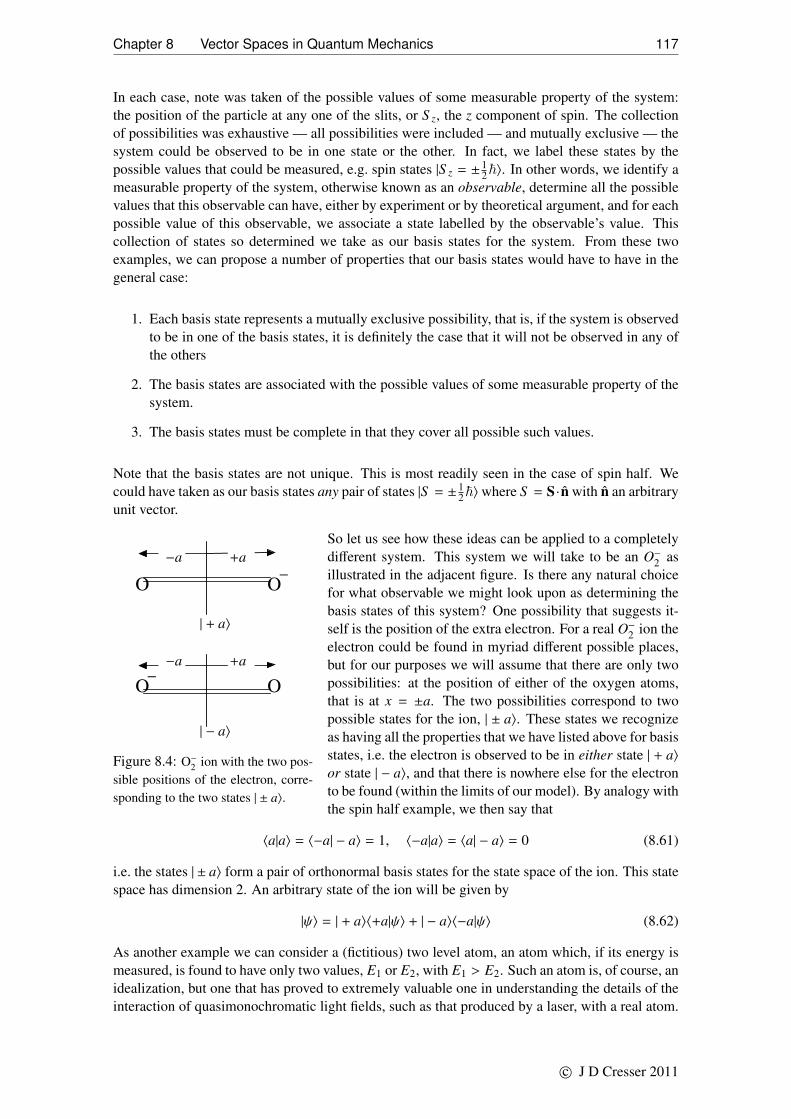
Chapter 8 Vector Spaces in Quantum Mechanics 117
In each case, note was taken of the possible values of some measurable property of the system:the position of the particle at any one of the slits, or S z, the z component of spin. The collectionof possibilities was exhaustive — all possibilities were included — and mutually exclusive — thesystem could be observed to be in one state or the other. In fact, we label these states by thepossible values that could be measured, e.g. spin states |S z = ± 1
2~〉. In other words, we identify ameasurable property of the system, otherwise known as an observable, determine all the possiblevalues that this observable can have, either by experiment or by theoretical argument, and for eachpossible value of this observable, we associate a state labelled by the observable’s value. Thiscollection of states so determined we take as our basis states for the system. From these twoexamples, we can propose a number of properties that our basis states would have to have in thegeneral case:
1. Each basis state represents a mutually exclusive possibility, that is, if the system is observedto be in one of the basis states, it is definitely the case that it will not be observed in any ofthe others
2. The basis states are associated with the possible values of some measurable property of thesystem.
3. The basis states must be complete in that they cover all possible such values.
Note that the basis states are not unique. This is most readily seen in the case of spin half. Wecould have taken as our basis states any pair of states |S = ± 1
2~〉where S = S ·n with n an arbitraryunit vector.
−a +a
O− O
| − a〉
−a +a
O −O
| + a〉
Figure 8.4: O−2 ion with the two pos-sible positions of the electron, corre-sponding to the two states | ± a〉.
So let us see how these ideas can be applied to a completelydifferent system. This system we will take to be an O−2 asillustrated in the adjacent figure. Is there any natural choicefor what observable we might look upon as determining thebasis states of this system? One possibility that suggests it-self is the position of the extra electron. For a real O−2 ion theelectron could be found in myriad different possible places,but for our purposes we will assume that there are only twopossibilities: at the position of either of the oxygen atoms,that is at x = ±a. The two possibilities correspond to twopossible states for the ion, | ± a〉. These states we recognizeas having all the properties that we have listed above for basisstates, i.e. the electron is observed to be in either state | + a〉or state | − a〉, and that there is nowhere else for the electronto be found (within the limits of our model). By analogy withthe spin half example, we then say that
〈a|a〉 = 〈−a| − a〉 = 1, 〈−a|a〉 = 〈a| − a〉 = 0 (8.61)
i.e. the states | ± a〉 form a pair of orthonormal basis states for the state space of the ion. This statespace has dimension 2. An arbitrary state of the ion will be given by
|ψ〉 = | + a〉〈+a|ψ〉 + | − a〉〈−a|ψ〉 (8.62)
As another example we can consider a (fictitious) two level atom, an atom which, if its energy ismeasured, is found to have only two values, E1 or E2, with E1 > E2. Such an atom is, of course, anidealization, but one that has proved to extremely valuable one in understanding the details of theinteraction of quasimonochromatic light fields, such as that produced by a laser, with a real atom.
c© J D Cresser 2011

Chapter 8 Vector Spaces in Quantum Mechanics 118
The nature of the interaction is such that the atom behaves as if it has only two energy levels, sothat the simplification being considered here is taken as the basis of often used theoretical models.
Given that the energy can only have two values, and moreover that the energy is measured to beeither E1 or E2 in a way totally analogous to measuring a component of the spin of a spin halfsystem, we can then assign to the atom two possible states, call them |E1〉 and |E2〉, or |e〉 and |g〉,where e ≡ excited state and g ≡ ground state. We then have
〈e|e〉 = 〈g|g〉 = 1
〈e|g〉 = 〈g|e〉 = 0. (8.63)
These states then act as the orthonormal basis states of our two level atom, so that any state of thetwo level atom can be written as a linear combination
|ψ〉 = a|e〉 + b|g〉. (8.64)
8.4.1 A General Formulation
We will now see how these ideas can be applied to more general kinds of physical systems. Tobegin, we have to set up these basis states for the given system. So suppose we perform anexhaustive series of measurements of some observable property of the system – call it Q. Forexample, we could determine through which slits it is possible for an electron to pass in the twoslit experiment above in which case Q ≡ ‘the positions of the two slits’, or the possible valuesof the Z component of the spin of a particle, in which case Q ≡ S z, or the possible values of theposition of an electron on an O−2 ion, as discussed above, in which case Q ≡ ‘the position of theelectron on the O−2 ion’. The generic name given to Q is that it is an ‘observable’. We will givemany more examples of observables later in this Chapter, and look at the concept again in a laterChapter.
Whatever the system, what we mean by exhaustive is that we determine all the possible values thatthe observed quantity Q might have. For instance, we determine that, in the two slit interferenceexperiment, the electron can pass through, (that is, be observed to be at) the position of one or theother of the two slits, or that a spin half particle would be observed to have either of the valuesS z = ±1
2~, and no other value. Or for the O−2 ion, the electron can be found either on the atom atposition x = −a or on the atom at position x = +a. In general, for an arbitrary observable Q, letus represent these observed values by q1, q2, q3, . . . , qN , i.e. N in total, all of which will be realnumbers. Of course, there might be other observable properties of the system that we might beable to measure, but for the present we will suppose that we only need concern ourselves with justone. In keeping with the way that we developed the idea of state earlier, we then let |q1〉 representthe state for which Q definitely has the value q1, and similarly for all the others possibilities.
We now turn to Eq. (7.48), the result obtained earlier when considering generalizations of thetwo slit experiment to the multiple slit case, or the generalization of the Stern-Gerlach experimentto the arbitrary spin case. There, a sum was made over probability amplitudes for the different‘pathways’ from a given initial state |ψ〉 to some final state |φ〉 via a set of intermediate slit or spinstates. Here, we generalize that result for an arbitrary set of intermediate states {|q1〉, |q2〉, . . .} asdefined above, and make the following claim, the fundamental rule of quantum mechanics, that ifthe system is initially prepared in the state |ψ〉, then the probability amplitude of finding it in thestate |φ〉 is given by
〈φ|ψ〉 =
N∑n=1
〈φ|qn〉〈qn|ψ〉 (8.65)
which tells us that the total probability amplitude of finding the system in the final state |φ〉 is justthe sum of the probability amplitudes of the system ‘passing through’ any of the states {|qn〉; n =
c© J D Cresser 2011

Chapter 8 Vector Spaces in Quantum Mechanics 119
1, 2, . . . ,N}. The expression Eq. (8.65) is often referred to as a closure relation though confusingly,it is also sometimes referred to as a completeness relation, a term which we apply to anotherexpression below.
We further claim, from the basic meaning of probability amplitude, that for any state |ψ〉 of thesystem, we must have
〈ψ|ψ〉 = 1 (8.66)
known as the normalization condition. This follows from the requirement that |〈ψ|ψ〉|2 = 1, i.e.that if the system is in the state |ψ〉, then it is definitely (i.e. with probability one) in the state |ψ〉.
We then recognize that the probability amplitudes 〈qm|qn〉 must have the following properties:
• 〈qm|qn〉 = 0 if m , n. This amounts to stating that if the system is in the state |qn〉, i.e.wherein the observable Q is known to have the value qn, then there is zero possibility offinding it in the state |qm〉. Thus the states {|qn〉; n = 1, 2, . . . ,N} are mutually exclusive.
• 〈qn|qn〉 = 1. This asserts that if the system is in the state for which the quantity Q has thevalue qn, then it is certain to be found in the state in which it has the value qn.
• The states {|qn〉; n = 1, 2, . . . ,N} are also exhaustive in that they cover all the possible valuesthat could be observed of the observable Q. These states are said to be complete — simplybecause they cover all possibilities.
These three properties are analogous to the properties that we associate with the inner products ofmembers of an orthonormal set of basis vectors for a complex inner product space, which suggestswe interpret the states {|qn〉; n = 1, 2, . . . ,N} as an orthonormal set of basis vectors, or basis states,for our system. We then interpret that fundamental law, Eq. (8.65) as an expression for the innerproduct of two state vectors, |ψ〉 and |φ〉 in terms of the components of these vectors with respectto the basis states |qn〉. Expressions for these state vectors in terms of the basis states can then beobtained by what we have referred to earlier as the ‘cancellation trick’ to give
|ψ〉 =
N∑n=1
|qn〉〈qn|ψ〉
〈φ| =
N∑n=1
〈φ|qn〉〈qn|
. (8.67)
We have argued above that the states {|qn〉; n = 1, 2, . . . ,N} are, in a sense, complete. We can usethis to argue that any state of the system can be expressed in the form Eq. (8.67). To see howthis follows, suppose |ψ〉 is some arbitrary state of the system. Then, for at least one of the states|qn〉, we must have 〈qn|ψ〉 , 0, i.e. we must have a non-zero probability of observing the system inone of the states |qn〉. If this were not the case, then for the system in a state such as |ψ〉 it wouldbe saying that if we measure Q, we don’t get an answer! This does not make physical sense. Sophysical consistency means that it must be the case that any state of the system can be written asin Eq. (8.67) and for that reason, these expressions are referred to as completeness relations.
We can also make the inverse claim that any such linear combination represents a possible state ofthe system. The justification for this is not as clear cut as there are physical systems for which thereare limitations on allowed linear combinations (so-called super-selection rules), but it appears tobe a rule that holds true unless there are good physical reasons, on a case-by-case basis, why itshould not. We will assume it to be true here.
c© J D Cresser 2011
Chapter 8 Vector Spaces in Quantum Mechanics 120
If we choose |φ〉 = |ψ〉 in Eq. (8.65) and we use the normalization condition we find that
〈ψ|ψ〉 =
N∑n=1
〈ψ|qn〉〈qn|ψ〉 = 1. (8.68)
But we must also have, since the probability of finding the system in any of the states |qn〉 mustadd up to unity that ∑
n
|〈qn|ψ〉|2 = 1 (8.69)
This can also be understood as being a consequence of our interpretation of the states {|qn〉; n =
1, 2, . . .N} as a complete set of mutually exclusive possibilities, complete in the sense that the totalprobability of ending up in any of the mutually exclusive possible final states |qn〉 adds up to unity— there is nowhere else for the system to be found. By subtracting the last two expressions wearrive at
N∑n=1
(〈ψ|qn〉 − 〈qn|ψ〉
∗) 〈qn|ψ〉 = 0. (8.70)
A sufficient condition for this result to hold true is
〈ψ|qn〉 = 〈qn|ψ〉∗ (8.71)
and hence that, in general,〈φ|ψ〉 = 〈ψ|φ〉∗. (8.72)
Thus, by a simple extension of the arguments presented in Section 8.3 in the case of spin halfquantum states it can be seen that the general results above are also completely analogous to theproperties of vectors in a complex vector space. This mathematical formalism will be discussedmore fully in the next Chapter, but for the present we can summarize the essential ideas based onwhat we have already put forward earlier. The important points then are as follows:
1. The collection of all the possible state vectors of a quantum system forms a complex vectorspace known as the state space of the system.
2. The probability amplitudes are identified as the inner product of these state vectors.
3. The intermediate states {|qn〉; n = 1, 2, . . . } form a complete orthonormal set of basis statesof this state space, i.e. any state vector |ψ〉 can be written as a linear combination of thesebasis states.
4. The number of basis states is known as the dimension of the state space.
8.4.2 Further Examples of State Spaces
The ideas developed above can now be applied to constructing a state space for a physical system.The basic idea is as discussed in Section 7.4 which enables us to define a set of basis states forthe state space of the system. By establishing a set of basis states, in a sense, we ‘bring the statespace into existence’, and once this is done, we are free to use all the mathematical machineryavailable for analysing the properties of the state space so constructed. The question can be askedas to whether or not the ideas presented in Section 7.4, admittedly extracted from only a handfulof examples, can be applied with success to any other system. This is a question that can only beanswered by applying the rules formulated there and considering the consequences. In Section 8.5we will discuss where these ideas, if naively applied, fail to work. Otherwise, these ideas, whenfully formed, constitute the basis of quantum physics.
c© J D Cresser 2011

Chapter 8 Vector Spaces in Quantum Mechanics 121
In accordance with the ideas developed in Section 7.4, constructing a state space for a physicalsystem can be carried out by recognizing the intermediate states through which a system can passas it makes its way from some initial state to some observed final state, as was done in the case ofthe two slit, or spin half systems. Thus, in the two slit example, the two possible intermediate statesare those for which the particle is to be found at the position of either of the two slits. In the spinhalf example, the two intermediate states are those in which the spin is observed to have either ofthe two values S z = ± 1
2~; these are the states we have been calling |±〉. These intermediate statesare states of the system that can be identified through an argument based on the idea that somephysical property of the system can be exhaustively measured to yield a set of values that we thenuse to label a complete set of basis states for the state space of the system.
Negatively Charged Ions Here the system is a molecule which has acquired an extra electron,which can be assumed to found only on any one of the atoms making up the molecule. This is, ofcourse, an approximation. The electron could be found anywhere around the atoms, or in the spacebetween the atoms, in a way that depends on the nature of the chemical bond between the atoms.Here we are making use of a coarse notion of position, i.e. we are assuming that the electron canbe observed to reside on one atom or the other, and we do not really care about exactly where oneach atom the electron might be found. The idea is best illustrated by the simple example of theO−2 ion in which the electron can be found on one or the other of the oxygen atoms (see Fig. (8.4))as discussed on p117.
This kind of model can be generalized to situations involving different geometries, such as atomsarranged in a ring e.g. an ozone ion O−3 . In this case, the state space will be spanned by three basisstates corresponding to the three possible positions at which the electron can be observed. Thismodel (and its generalizations to an arbitrary number of atoms arranged in a ring) is valuable asit gives rise to results that serve as an approximate treatment of angular momentum in quantummechanics.
Spin Flipping In this case, we have a spin half particle (for instance) in a constant magneticfield, so the two possible states are the familiar spin up or spin down states. If, in addition, weadd a rotating magnetic field at right angles to the constant field, there arises a time dependentprobability of the spin flipping from one orientation to the other. As the spin up and spin downstates are of different energies, this represents a change in energy of the particle, a change that canbe detected, and is the basis of the electron spin and nuclear magnetic resonance imaging muchused in medical work. Obviously this is a state space of dimension two.
Ammonia molecule Here the system is theammonia molecule NH3 in which the nitro-gen atom is at the apex of a triangular pyra-mid with the three hydrogen atoms formingan equilateral triangle as the base. The ni-trogen atom can be positioned either aboveor below the plane of the hydrogen atoms,these two possibilities we take as two possi-ble states of the ammonia molecule. (The Natom can move between these two positionsby ‘quantum tunnelling’ through the poten-tial barrier lying in the plane of the hydrogenatoms.) Once again, this is a state space ofdimension 2.
+l−l
N
H
H
H
N
H
H H
Figure 8.5: Ammonia molecule in two states dis-tinguished by the position of the nitrogen atom,either above or below the plane of the hydrogenatoms, corresponding to the states | + l〉 and | − l〉respectively.
c© J D Cresser 2011
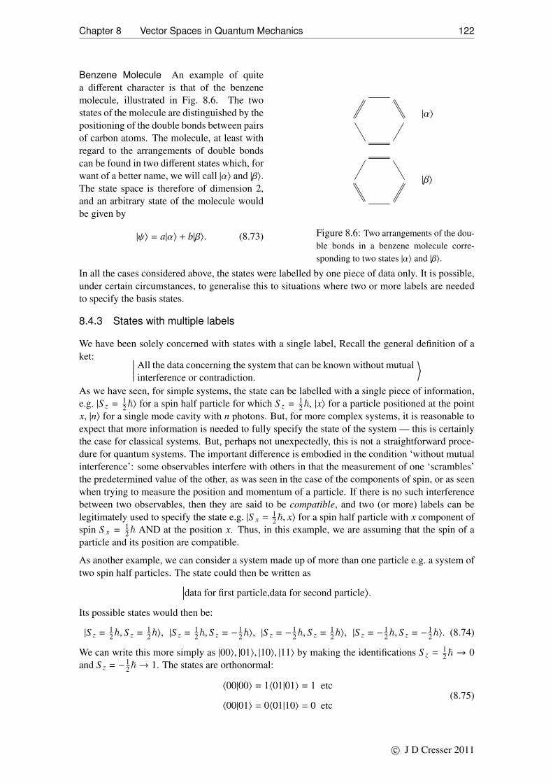
Chapter 8 Vector Spaces in Quantum Mechanics 122
Benzene Molecule An example of quitea different character is that of the benzenemolecule, illustrated in Fig. 8.6. The twostates of the molecule are distinguished by thepositioning of the double bonds between pairsof carbon atoms. The molecule, at least withregard to the arrangements of double bondscan be found in two different states which, forwant of a better name, we will call |α〉 and |β〉.The state space is therefore of dimension 2,and an arbitrary state of the molecule wouldbe given by
|ψ〉 = a|α〉 + b|β〉. (8.73)
|α〉
|β〉
Figure 8.6: Two arrangements of the dou-ble bonds in a benzene molecule corre-sponding to two states |α〉 and |β〉.
In all the cases considered above, the states were labelled by one piece of data only. It is possible,under certain circumstances, to generalise this to situations where two or more labels are neededto specify the basis states.
8.4.3 States with multiple labels
We have been solely concerned with states with a single label, Recall the general definition of aket: ∣∣∣∣∣ All the data concerning the system that can be known without mutual
interference or contradiction.
⟩As we have seen, for simple systems, the state can be labelled with a single piece of information,e.g. |S z = 1
2~〉 for a spin half particle for which S z = 12~, |x〉 for a particle positioned at the point
x, |n〉 for a single mode cavity with n photons. But, for more complex systems, it is reasonable toexpect that more information is needed to fully specify the state of the system — this is certainlythe case for classical systems. But, perhaps not unexpectedly, this is not a straightforward proce-dure for quantum systems. The important difference is embodied in the condition ‘without mutualinterference’: some observables interfere with others in that the measurement of one ‘scrambles’the predetermined value of the other, as was seen in the case of the components of spin, or as seenwhen trying to measure the position and momentum of a particle. If there is no such interferencebetween two observables, then they are said to be compatible, and two (or more) labels can belegitimately used to specify the state e.g. |S x = 1
2~, x〉 for a spin half particle with x component ofspin S x = 1
2~ AND at the position x. Thus, in this example, we are assuming that the spin of aparticle and its position are compatible.
As another example, we can consider a system made up of more than one particle e.g. a system oftwo spin half particles. The state could then be written as∣∣∣data for first particle,data for second particle
⟩.
Its possible states would then be:
|S z = 12~, S z = 1
2~〉, |S z = 12~, S z = − 1
2~〉, |S z = − 12~, S z = 1
2~〉, |S z = − 12~, S z = − 1
2~〉. (8.74)
We can write this more simply as |00〉, |01〉, |10〉, |11〉 by making the identifications S z = 12~ → 0
and S z = − 12~→ 1. The states are orthonormal:
〈00|00〉 = 1〈01|01〉 = 1 etc
〈00|01〉 = 0〈01|10〉 = 0 etc(8.75)
c© J D Cresser 2011

Chapter 8 Vector Spaces in Quantum Mechanics 123
An arbitrary state is |ψ〉 = a|00〉 + b|01〉 + c|10〉 + d|11〉. These states form a set of orthonormalbasis states for a state space of dimension 4. The idea can be extended to many particles, or othermore complex systems e.g. whole atoms, or molecules or solid state systems and so on.
The notion of ‘compatible observables’ and determining whether or not two (or more) observablesare compatible, is studied later in a more rigorous way once the idea of an observable beingrepresented by Hermitean operators has been formulated.
Qubits Note that a single spin half has the basis states |0〉 and |1〉 in our new notation. These twostates can be looked on as corresponding to the two binary numbers 0 and 1. A linear combination
|ψ〉 = c0|0〉 + c1|1〉.
can be formed which represents the possibility of a memory registering a bit of information simul-taneously as both a 0 and a 1. This is in contrast with a classical bit, which can be registered aseither a 0 or a 1. The spin half system is an example of a qubit. But spin half is not in any wayspecial: any two state system: a spin half particle, a two level atom, the two configurations of abenzene molecule, a quantum dot either occupied or not occupied by an electron . . . . Quantumcomputation then involves manipulating the whole state |ψ〉, which, in effect, amounts to perform-ing two calculations at once, differing by the initial setting of the memory bit.
This idea introduced can be readily extended. Thus, if we have two spin half particles, we havethe possible states |00〉, |01〉, |10〉, and |11〉. The data labelling the state |00〉 represents the numberzero, |01〉 the number one, |10〉 the number two, and |11〉 the number three. We now have twoqubits, and a state space of dimension four, and we can set up linear combinations such as
|ψ〉 = c00|00〉 + c01|01〉 + c10|10〉 + c11|11〉 (8.76)
and we can then perform calculations making use, simultaneously, of four different possible valuesfor whatever quantity the states are intended to represent. With three atoms, or four and so on, thestate space becomes much larger: of dimension 2N in fact where N is the number of qubits, andthe basis states represent the numbers ranging from 0 to 2N − 1 in binary notation.
The viability of this scheme relies on the linear combination not being destroyed by decoherence.Decoherence is the consequence of noise destroying a linear combination of quantum states, turn-ing a quantum state into a mixture of alternate classical possibilities.
8.5 States of Macroscopic Systems — the role of decoherence
In the examples given above, it was assumed that an exhaustive list of results that could be obtainedin the measurement of some observable of a quantum system could be used to set up the basisstates for the state space of the system. The value of doing this is, of course, to be determineby the success or otherwise of these ideas. That quantum mechanics is such an overwhelminglysuccessful theory indicates that there is something correct in this procedure, but the question thatarises is this: why does it not appear to work for macroscopic systems, i.e. for systems whichwe know can be fully adequately explained by standard classical physics? The answer appearsto lie in the fact that in all the examples discussed above, whether or not the Hilbert space is offinite or infinite dimension, i.e. whether or not we are talking about spin up or spin down of aspin half particle, or the position of a particle in space, the implicit assumption is that the systemwe are considering is totally isolated from all other systems, in particular from any influence ofthe surrounding environment. After all, when we talked about a system, such as an O−2 ion, weare ignoring all the other physical influences that could act on this system, i.e. we do not need tomention, in our specification of the state of the system, anything other than properties that directlypertain to the system of interest. The assumption is made, as it is in classical physics, that such
c© J D Cresser 2011

Chapter 8 Vector Spaces in Quantum Mechanics 124
influences are sufficiently weak that they can be ignored to a good approximation. In effect, weare supposing that the systems under consideration are isolated systems, that is, systems that areisolated from the effect of any external perturbations.
Classically, at the macroscopic level, we can usually continue to ignore weak perturbing influenceswhen specifying the state of a system. In fact, when defining a ‘system’ we typically include inwhat we refer to as the ‘system’, all the participants in the physical process being described thatinteract strongly with each other. Anything else that weakly affects these constituents is ignored.For instance, when describing the orbital dynamics of the Earth as it revolves around the Sun, wemight need to take into account the gravitational pull of the Moon – the system is the Earth, theSun and the Moon. But we do not really need to take into account the effect of the backgroundmicrowave radiation left over after the Big Bang. Or, when describing the collision between twobilliard balls, it is probably necessary to include the effect of rolling friction, but it not reallynecessary to take into account the frictional drag due to air resistance. Of course, sometimesit is necessary to include external influences even when weak: to describe a system coming tothermal equilibrium with its surroundings it is necessary to extend the system by including theenvironment in the dynamical model. In any of these examples, the same classical physics methodsand philosophy applies.
There is a subtle difference when it comes to trying to apply the quantum ideas developed so farto macroscopic systems. The same, weak perturbations that can be put to one side in a classicaldescription of a macroscopic system turn out to have a far-reaching effect if included in a quantumdescription of the same system. If we were to attempt to describe a macroscopic system accordingto the laws of quantum mechanics, we would find that any linear superposition of different possiblestates of the system evolves on a fantastically short time scale to a classical mixture of the differentpossibilities. For instance, if we were to attempt to describe the state of a set of car keys in termsof two possibilities: in your pocket |p〉 or in your brief case |b〉, then a state of the form
|ψ〉 =1√
2
(|p〉 + |b〉
)(8.77)
could be used to represent a possible ‘quantum state’ of the keys. But this quantum state would beexceedingly short lived (on a time scale ∼ 10−40 sec), and would evolve into the two alternativepossibilities: a 50% chance of the keys being in the state |p〉, i.e. a 50% chance of finding yourkeys in your pocket, and a 50% chance of being in the state |b〉, i.e. a 50% chance of finding themin your brief case. But this is no longer a superposition of these two states. Instead, the keys areeither in the state |p〉 or the state |b〉. What this effectively means is that randomness is still there,i.e. repeating an experiment under identical conditions can give randomly varying results. But thestate of the keys is no longer represented by a state vector, so there are no longer any quantuminterference effects present. The randomness can then be looked upon as being totally classical innature, i.e. as being due to our ignorance of information that is in principle there, but impossiblydifficult to access. In effect, the quantum system behaves like a noisy classical system.
The process that washes out the purely quantum effects is known as decoherence. Since it iseffectively impossible to isolate any macroscopic system from the influence of its surroundingenvironment1, all macroscopic systems are subject to decoherence. This process is believed toplay a crucial role in why, at the macroscopic level, physical systems, which are all intrinsicallyquantum mechanical, behave in accordance with the classical laws of physics. It is also one ofthe main corrupting influences that prevent a quantum computer from functioning as it should.Quantum computers rely for their functioning on the ‘qubits’ remaining in linear superpositions ofstates, but the ever-present decohering effects of the environment will tend to destroy these delicatequantum states before a computation is completed, or else at the very least introduce errors as the
1‘No man is an Iland, intire of itselfe’ – J. Donne, Devotions upon Emergent Occasions Meditation XVII (1693)
c© J D Cresser 2011

Chapter 8 Vector Spaces in Quantum Mechanics 125
computation proceeds. Controlling decoherence is therefore one of the major challenges in thedevelopment of viable quantum computers.
So, the bottom line is that it is only for protected isolated systems that quantum effects are mostreadily observed, and it is for microscopic systems that this state of affairs is to be found. Butthat is not to say that quantum effects are not present at the macroscopic level. Peculiar quantumeffects associated with the superposition of states are not to be seen, but the properties of matter ingeneral, and indeed the properties of the forces of nature, are all intrinsically quantum in origin.
c© J D Cresser 2011

Chapter 9
General Mathematical Description of a QuantumSystem
It was shown in preceding Chapter that the mathematical description of this sum of probabilityamplitudes admits an interpretation of the state of the system as being a vector in a complex
vector space, the state space of the system. It is this mathematical picture that is summarizedhere in the general case introduced there. This idea that the state of a quantum system is to beconsidered a vector belonging to a complex vector space, which we have developed here in thecase of a spin half system, and which has its roots in the sum over paths point of view, is the basisof all of modern quantum mechanics and is used to describe any quantum mechanical system.Below is a summary of the main points as they are used for a general quantum system whose statespaces are of arbitrary dimension (including state spaces of infinite dimension). The emphasishere is on the mathematical features of the theory.
9.1 State Space
We have indicated a number of times that in quantum mechanics, the state of a physical systemis represented by a vector belonging to a complex vector space known as the state space of thesystem. Here we will give a list of the defining conditions of a state space, though we will not beconcerning ourselves too much with the formalities. The following definitions and concepts set upthe state space of a quantum system.
1. Every physical state of a quantum system is specified by a symbol knonw as a ket written| . . .〉 where . . . is a label specifying the physical information known about the state. Anarbitrary state is written |ψ〉, or |φ〉 and so on.
2. The set of all state vectors describing a given physical system forms a complex inner productspace H (actually a Hilbert space, see Sec. 9.2) also known as the state space or ket spacefor the system. A ket is also referred to as a state vector, ket vector, or sometimes just state.
Thus every linear combination (or superposition) of two or more state vectors |φ1〉, |φ2〉,|φ3〉, . . . , is also a state of the quantum system i.e. the state |ψ〉 given by
|ψ〉 = c1|φ1〉 + c2|φ2〉 + c3|φ3〉 + . . .
is a state of the system for all complex numbers c1, c2, c3, . . . .
This last point amounts to saying that every physical state of a system is represented by a vectorin the state space of the system, and every vector in the state space represents a possible physicalstate of the system. To guarantee this, the following condition is also imposed:
c© J D Cresser 2011

Chapter 9 General Mathematical Description of a Quantum System 127
3. If a physical state of the system is represented by a vector |ψ〉, then the same physical stateis represented by the vector c|ψ〉 where c is any non-zero complex number.
Next, we need the concept of completeness:
4. A set of vectors |ϕ1〉, |ϕ2〉, |ϕ3〉, . . . is said to be complete if every state of the quantum systemcan be represented as a linear combination of the |ϕi〉’s, i.e. for any state |ψ〉 we can write
|ψ〉 =∑
i
c1|ϕi〉.
The set of vectors |ϕi〉 are said to span the space.
For example, returning to the spin half system, the two states |±〉 are all that is needed to describeany state of the system, i.e. there are no spin states that cannot be described in terms of these basisstates. Thus, these states are said to be complete.
Finally, we need the concept of a set of basis states, and of the dimension of the state space.
5. A set of vectors {|ϕ1〉, |ϕ2〉, |ϕ3〉, . . . } is said to form a basis for the state space if the set ofvectors is complete, and if they are linearly independent. The vectors are also termed thebase states for the vector space.
Linear independence means that if∑
i
ci|ϕi〉 = 0 then ci = 0 for all i.
The states |±〉 for a spin half system can be shown to be linearly independent, and thus form abasis for the state space of the system.
6. The minimum number of vectors needed to form a complete set of basis states is knownas the dimension of the state space. [In many, if not most cases of interest in quantummechanics, the dimension of the state space is infinite.]
It should be noted that there is an infinite number of possible sets of basis states for any state space.The arguments presented in the preceding Chapter by which we arrive at a set of basis states servesas a physically motivated starting point to construct the state space for the system. But once wehave defined the state space in this way, there is no reason why we cannot, at least mathematically,construct other sets of basis states. These basis states that we start with are particularly useful asthey have an immediate physical meaning; this might not be the case for an arbitrary basis set.But there are other means by which other physically meaningful basis states can be determined:often the choice of basis states is suggested by the physics (such as the set of eigenstates of anobservable, see Chapter 11).
9.2 Probability Amplitudes and the Inner Product of State Vectors
We obtained a number of properties of probability amplitudes when looking at the case of a spinhalf system. Some of the results obtained there, and a few more that were not, are summarized inthe following.
If |φ〉 and |ψ〉 are any two state vectors belonging to the state spaceH , then
1. 〈φ|ψ〉, a complex number, is the probability amplitude of observing the system to be in thestate |φ〉 given that it is in the state |ψ〉.
c© J D Cresser 2011

Chapter 9 General Mathematical Description of a Quantum System 128
2. The probability of observing the system to be in the state |φ〉 given that it is in the state |ψ〉is |〈φ|ψ〉|2.
The probability amplitude 〈φ|ψ〉, can then be shown to have the properties
3. 〈φ|ψ〉 = 〈ψ|φ〉∗.
4. 〈φ|{c1|ψ1〉 + c2|ψ2〉} = c1〈φ|ψ1〉 + c2〈φ|ψ2〉 where c1 and c2 are complex numbers.
5. 〈ψ|ψ〉 ≥ 0. If 〈ψ|ψ〉=0 then |ψ〉 = 0, the zero vector.
This last statement is related to the physically reasonable requirement that the probability of asystem being found in a state |ψ〉 given that it is in the state |ψ〉 has to be unity, i.e. |〈ψ|ψ〉|2 = 1which means that 〈ψ|ψ〉 = exp(iη). We now choose η = 0 so that 〈ψ|ψ〉 = 1. But recall that anymultiple of a state vector still represents the same physical state of the system, i.e. |ψ〉 = a|ψ〉still represents the same physical state as |ψ〉. However, in this case, 〈ψ|ψ〉 = |a|2 which is notnecessarily unity, but is is certainly bigger than zero.
6. The quantity√〈ψ|ψ〉 is known as the length or norm of |ψ〉.
7. A state |ψ〉 is normalized, or normalized to unity, if 〈ψ|ψ〉 = 1.
Normalized states are states which have a direct probability interpretation. It is mathematicallyconvenient to permit the use of states whose norms are not equal to unity, but it is necessary inorder to make use of the probability interpretation to deal only with the normalized state whichhas norm of unity. Any state that cannot be normalized to unity (i.e. it is of infinite length) cannotrepresent a physically acceptable state.
8. Two states |φ〉 and |ψ〉 are orthogonal if 〈φ|ψ〉 = 0.
The physical significance of two states being orthogonal should be understood: for a system in acertain state, there is zero probability of it being observed in a state with which it is orthogonal. Inthis sense, two orthogonal states are as distinct as it is possible for two states to be.
Finally, a set of orthonormal basis vectors {|ϕn〉; n = 1, 2, . . . } will have the property
9. 〈ϕm|ϕn〉 = δmn where δmn is known as the Kronecker delta, and equals unity if m = n andzero if m , n.
All the above conditions satisfied by probability amplitudes were to a greater or lesser extent phys-ically motivated, but it nevertheless turns out that these conditions are identical to the conditionsthat are used to define the inner product of two vectors in a complex vector space, in this case,the state space of the system, i.e. we could write, using the usual mathematical notation for aninner product, 〈φ|ψ〉 = (|φ〉, |ψ〉). The state space of a physical system is thus more than just acomplex vector space, it is a vector space on which there is defined an inner product, and so ismore correctly termed a complex ‘inner product’ space. Further, it is usually required in quantummechanics that certain convergency criteria, defined in terms of the norms of sequences of vectorsbelonging to the state space, must be satisfied. This is not of any concern for spaces of finite di-mension, but are important for spaces of infinite dimension. If these criteria are satisfied then thestate space is said to be a Hilbert space. Thus rather than referring to the state space of a system,reference is made to the Hilbert space of the system.
c© J D Cresser 2011

Chapter 9 General Mathematical Description of a Quantum System 129
What this means, mathematically, is that for every state |φ〉 say, at least one of the inner products〈ϕn|φ〉 will be non-zero, or conversely, there does not exist a state |ξ〉 for which 〈ϕn|ξ〉 = 0 for allthe basis states |ϕn〉. Completeness clearly means that no more basis states are needed to describeany possible physical state of a system.
It is important to recognize that all the vectors belonging to a Hilbert space have finite norm, or,putting it another way, all the state vectors can be normalized to unity – this state of affairs isphysically necessary if we want to be able to apply the probability interpretation in a consistentway. However, as we shall see, we will encounter states which do not have a finite norm and henceneither represent physically realizable states, nor do they belong to the state or Hilbert space ofthe system. Nevertheless, with proper care regarding their use and interpretation, such states turnout to be essential, and play a crucial role throughout quantum mechanics.
Recognizing that a probability amplitude is nothing but an inner product on the state space of thesystem, leads to a more general way of defining what is meant by a bra vector. The followingdiscussion emphasizes the fact that a bra vector, while it shares many characteristices of a ketvector, is actually a different mathematical entity.
9.2.1 Bra Vectors
We have consistently used the notation 〈φ|ψ〉 to represent a probability amplitude, but we havejust seen that this quantity is in fact nothing more than the inner product of two state vectors,which can be written in a different notation, (|φ〉, |ψ〉), that is more commonly encountered inpure mathematics. But the inner product can be viewed in another way, which leads to a newinterpretation of the expression 〈φ|ψ〉, and the introduction of a new class of state vectors. If weconsider the equation
〈φ|ψ〉 = (|φ〉, |ψ〉) (9.1)
and ‘cancel’ the |ψ〉, we get the result
〈φ| • = (|φ〉, •) (9.2)
where the ‘•’ is inserted, temporarily, to remind us that in order to complete the equation, a ketvector has to be inserted. By carrying out this procedure, we have introduced a new quantity 〈φ|which is known as a bra or bra vector, essentially because 〈φ|ψ〉 looks like quantities enclosedbetween a pair of ‘bra(c)kets’. It is a vector because, as can be readily shown, the collection of allpossible bras form a vector space. For instance, by the properties of the inner product, if
|ψ〉 = a1|ϕ1〉 + a2|ϕ2〉 (9.3)
then
(|ψ〉, •) = 〈ψ| • = (a1|ϕ1〉 + a2|ϕ2〉, •) (9.4)
= a∗1(|ϕ1〉, •) + a∗2(|ϕ2〉, •) = a∗1〈ϕ1| • + a∗2〈ϕ2| • (9.5)
i.e., dropping the ‘•’ symbols, we have
〈ψ| = a∗1〈ϕ1| + a∗2〈ϕ2| (9.6)
so that a linear combination of two bras is also a bra, from which follows (after a bit more workchecking that the other requirements of a vector space are also satisfied) the result that the setof all bras is a vector space. Incidentally, this last calculation above shows, once again, that if|ψ〉 = a1|ϕ1〉 + a2|ϕ2〉 then the corresponding bra is 〈ψ| = a∗1〈ϕ1| + a∗2〈ϕ2|. So, in a sense, the bravectors are the ‘complex conjugates’ of the ket vectors.
c© J D Cresser 2011

Chapter 9 General Mathematical Description of a Quantum System 130
The vector space of all bra vectors is obviously closely linked to the vector space of all the ketsH , and is in fact usually referred to as the dual space, and represented byH∗. To each ket vector|ψ〉 belonging to H , there is then an associated bra vector 〈ψ| belonging to the dual space H∗.However, the reverse is not necessarily true: there are bra vectors that do not necessarily have acorresponding ket vector, and therein lies the difference between bras and kets. It turns out thatthe difference only matters for Hilbert spaces of infinite dimension, in which case there can arisebra vectors whose corresponding ket vector is of infinite length, i.e. has infinite norm, and hencecannot be normalized to unity. Such ket vectors can therefore never represent a possible physicalstate of a system. But these issues will not be of any concern here. The point to be taken awayfrom all this is that a bra vector is not the same kind of mathematical object as a ket vector. In fact,it has all the attributes of an operator in the sense that it acts on a ket vector to produce a complexnumber, this complex number being given by the appropriate inner product. This is in contrastto the more usual sort of operators encountered in quantum mechanics that act on ket vectors toproduce other ket vectors. In mathematical texts a bra vector is usually referred to as a ‘linearfunctional’. Nevertheless, in spite of the mathematical distinction that can be made between braand ket vectors, the correspondence between the two kinds of vectors is in most circumstances socomplete that a bra vector equally well represents the state of a quantum system as a ket vector.Thus, we can talk of a system being in the state 〈ψ|.
We can summarize all this in the general case as follows: The inner product (|ψ〉, |φ〉) defines, forall states |ψ〉, the set of functions (or linear functionals) (|ψ〉, ). The linear functional (|ψ〉, ) mapsany ket vector |φ〉 into the complex number given by the inner product (|ψ〉, |φ〉).
1. The set of all linear functionals (|ψ〉, ) forms a complex vector spaceH∗, the dual space ofH .
2. The linear functional (|ψ〉, ) is written 〈ψ| and is known as a bra vector.
3. To each ket vector |ψ〉 there corresponds a bra vector 〈ψ| such that if |φ1〉 → 〈φ1| and |φ2〉 →
〈φ2| thenc1|φ1〉 + c2|φ2〉 → c∗1〈φ1| + c∗2〈φ2|.
c© J D Cresser 2011
Chapter 10
State Spaces of Infinite Dimension
So far we have limited the discussion to state spaces of finite dimensions, but it turns out that, inpractice, state spaces of infinite dimension are fundamental to a quantum description of almost
all physical systems. The simple fact that a particle moving in space requires for its quantummechanical description a state space of infinite dimension shows the importance of being ableto work with such state spaces. This would not be of any concern if doing so merely requiredtransferring over the concepts already introduced in the finite case, but infinite dimensional statespaces have mathematical peculiarities and associated physical interpretations that are not foundin the case of finite dimension state spaces. Some of these issues are addressed in this Chapter,while other features of infinite dimensional state spaces are discussed as the need arises in laterChapters.
10.1 Examples of state spaces of infinite dimension
All the examples given in Chapter 8 yield state spaces of finite dimension. Much the same argu-ment can be applied to construct state spaces of infinite dimension. A couple of examples follow.
The Tight-Binding Model of a Crystalline Metal The examples given above of an electron beingpositioned on one of a (finite) number of atoms can be readily generalized to a situation in whichthere are an infinite number of such atoms. This is not a contrived model in any sense, as it is agood first approximation to modelling the properties of the conduction electrons in a crystallinesolid. In the free electron model of a conducting solid, the conduction electrons are assumedto be able to move freely (and without mutual interaction) through the crystal, i.e. the effects ofthe background positive potentials of the positive ions left is ignored. A further development ofthis model is to take into account the fact that the electrons will experience some attraction tothe periodically positioned positive ions, and so there will be a tendency for the electrons to befound in the neighbourhood of these ions. The resultant model – with the basis states consistingof a conduction electron being found on any one of the ion sites – is obviously similar to theone above for the molecular ion. Here however, the number of basis states is infinite (for aninfinite crystal), so the state space is of infinite dimension. Representing the set of basis states by{|n〉, n = 0,±1,±2, . . . } where na is the position of the nth atom, and a is the separation betweenneighbouring atoms, then any state of the system can then be written as
|ψ〉 =
+∞∑n=−∞
cn|n〉. (10.1)
By taking into account the fact that the electrons can make their way from an ion to one of itsneighbours, much of the band structure of semiconducting solids can be obtained.
c© J D Cresser 2011

Chapter 10 State Spaces of Infinite Dimension 132
Free Particle We can generalize the preceding model by supposing that the spacing betweenthe neighbouring atoms is allowed to go to zero, so that the positions at which the electron canbe found become continuous. This then acts as a model for the description of a particle free tomove anywhere in one dimension, and is considered in greater detail later in Section 10.2.2. Insetting up this model, we find that as well as there being an infinite number of basis states —something we have already encountered — we see that these basis states are not discrete, i.e. aparticle at position x will be in the basis state |x〉, and as x can vary continuously over the range−∞ < x < ∞, there will be a non-denumerably infinite, that is, a continuous range of such basisstates. As a consequence, the completeness relation ought to be written as an integral:
|ψ〉 =
∫ +∞
−∞
|x〉〈x|ψ〉 dx. (10.2)
The states |x〉 and |x′〉 will be orthonormal if x , x′, but in order to be able to retain the complete-ness relation in the form of an integral, it turns out that these basis states have to have an infinitenorm. However, there is a sense in which we can continue to work with such states, as will bediscussed in Section 10.2.2.
Particle in an Infinitely Deep Potential Well We saw in Section 5.3 that a particle of mass m inan infinitely deep potential well of width L can have the energies En = n2π2~2/2mL2 where n is apositive integer. This suggests that the basis states of the particle in the well be the states |n〉 suchthat if the particle is in state |n〉, then it has energy En. The probability amplitude of finding theparticle at position x when in state |n〉 is then 〈x|n〉 which, from Section 5.3 we can identify withthe wave function ψn, i.e.
ψn(x) = 〈x|n〉 =
√2L
sin(nπx/L) 0 < x < L
= 0 x < 0, x > L. (10.3)
The state space is obviously of infinite dimension.
It has been pointed out before that a state space can have any number of sets of basis states, i.e. thestates |n〉 introduced here do not form the sole possible set of basis states for the state space of thissystem. In this particular case, it is worthwhile noting that we could have used as the base statesthe states labelled by the position of the particle in the well, i.e. the states |x〉.
As we have seen, there are an infinite number of such states which is to be expected as we havealready seen that the state space is of infinite dimension. But the difference between this set ofstates and the set of states |n〉 is that in the latter case, these states are discrete, i.e. they can belabelled by the integers, while the states |x〉 are continuous, they are labelled by the continuousvariable x. Thus, something new emerges from this example: for state spaces of infinite dimension,it is possible to have a denumerably infinite number of basis states (i.e. the discrete states |n〉) ornon-denumerably infinite number of basis states (i.e. the states |x〉.) This feature of state spaces ofinfinite dimension, plus others, are discussed separately below in Section 10.2.
A System of Identical Photons Many other features of a quantum system not related to the posi-tion or energy of the system can be used as a means by which a set of basis states can be set up. Animportant example is one in which the system consists of a possibly variable number of identicalparticles. One example is a ‘gas’ of photons, all of the same frequency and polarization. Such asituation is routinely achieved in the laboratory using suitably constructed hollow superconductingmetallic cavities designed to support just one mode (i.e. a single frequency and polarization) ofthe electromagnetic field. The state of the electromagnetic field can then be characterized by thenumber n of photons in the field which can range from zero to positive infinity, so that the statesof the field (known as number states) can be written |n〉 with n = 0, 1, 2, . . .. The state |0〉 is often
c© J D Cresser 2011

Chapter 10 State Spaces of Infinite Dimension 133
referred to as the vacuum state. These states will then constitute a complete, orthonormal set ofbasis states (called Fock or number states), i.e.
〈n|m〉 = δnm (10.4)
and as n can range up to infinity, the state space for the system will be infinite dimensional. Anarbitrary state of the cavity field can be then be written
|ψ〉 =
∞∑n=0
cn|n〉 (10.5)
so that |cn|2 will be the probability of finding n photons in the field. In terms of these basis states,
it is possible to describe the processes in which particles are created or destroyed. For instance ifthere is a single atom in an excited energy state in the cavity, and the cavity is in the vacuum state|0〉, then the state of the combined atom field system can be written |e, 0〉, where the e indicatesthat the atom is in an excited state. The atom can later lose this energy by emitting it as a photon,so that at some later time the state of the system will be a|e, 0〉 + b|g, 1〉, where now there is thepossibility, with probability |b|2, of the atom being found in its ground state, and a photon havingbeen created.
10.2 Some Mathematical Issues
Some examples of physical systems with state spaces of infinite dimension were provided in theprevious Section. In these examples, we were able to proceed, at least as far as constructing thestate space was concerned, largely as was done in the case of finite dimensional state spaces. How-ever, further investigation shows that there are features of the mathematics, and the correspondingphysical interpretation in the infinite dimensional case that do not arise for systems with finite di-mensional state spaces. Firstly, it is possible to construct state vectors that cannot represent a stateof the system and secondly, the possibility arises of the basis states being continuously infinite.This latter state of affairs is not at all a rare and special case — it is just the situation needed todescribe the motion of a particle in space, and hence gives rise to the wave function, and wavemechanics.
10.2.1 States of Infinite Norm
To illustrate the first of the difficulties mentioned above, consider the example of a system ofidentical photons in the state |ψ〉 defined by Eq. (10.5). As the basis states are orthonormal wehave for 〈ψ|ψ〉
〈ψ|ψ〉 =
∞∑n=0
|cn|2 (10.6)
If the probabilities |cn|2 form a convergent infinite series, then the state |ψ〉 has a finite norm, i.e.
it can be normalized to unity. However, if this series does not converge, then it is not possibleto supply a probability interpretation to the state vector as it is not normalizable to unity. Forinstance, if c0 = 0 and cn = 1/
√n, n = 1, 2, . . ., then
〈ψ|ψ〉 =
∞∑n=1
1n
(10.7)
which is a divergent series, i.e. this state cannot be normalized to unity. In contrast, if cn = 1/n, n =
1, 2, . . ., then
〈ψ|ψ〉 =
∞∑n=1
1n2 =
π2
6(10.8)
c© J D Cresser 2011

Chapter 10 State Spaces of Infinite Dimension 134
which means we can normalize this state to unity by defining
|ψ〉 =
√6π|ψ〉. (10.9)
This shows that there are some linear combination of states that do not represent possible physicalstates of the system. Such states do not belong to the Hilbert spaceH of the system, i.e. the Hilbertspace consists only of those states for which the coefficients cn satisfy Eq. (10.6) 1. This is a newfeature: the possibility of constructing vectors that do not represent possible physical states of thesystem. It turns out that some very useful basis states have this apparently undesirable property,as we will now consider.
10.2.2 Continuous Basis States
In Section 10.1 an infinite one-dimensional model of a crystal was used as an illustrative modelfor a state space of infinite dimension. We can now consider what happens if we suppose that theseparation between the neighbouring atoms in the crystal goes to zero, so that the electron can befound anywhere over a range extending from −∞ to ∞. This, in effect, is the continuous limit ofthe infinite crystal model just presented, and represents the possible positions that a particle freeto move anywhere in one dimension, the X axis say, can have.
In this case, we could label the possible states of the particle by its X position, i.e. |x〉, where now,instead of having the discrete values of the crystal model, the position can now assume any of acontinuous range of values, −∞ < x < ∞. It would seem that we could then proceed in the sameway as we have done with the discrete states above, but it turns out that such states cannot benormalized to unity and hence do not represent (except in an idealised sense) physically allowablestates of the system.
The aim here is to try to develop a description of the possible basis states for a particle that is notlimited to being found only at discrete positions on the X axis. After all, in principle, we wouldexpect that a particle in free space could be found at any position x in the range −∞ < x < ∞. Wewill get at this description by a limiting procedure which is not at all mathematically rigorous, butnevertheless yields results that turn out to be valid. Suppose we return to the completeness relationfor the states |na〉 for the one dimensional crystal
|ψ〉 =
+∞∑n=−∞
|na〉〈na|ψ〉. (10.10)
If we now put a = ∆x and na = xn, and write |na〉 =√
a|xn〉, this becomes
|ψ〉 =
+∞∑n=−∞
|xn〉〈xn|ψ〉∆x (10.11)
where now〈xn|xm〉 =
δnm
a(10.12)
1Note however, that we can still construct a bra vector
〈ψ| =
n=∞∑n=0
c∗n〈n|
without placing any restrictions on the convergence of the cn’s such as the one in Eq. (10.6). The corresponding ketcannot then represent a possible state of the system, but such inner products as 〈ψ|φ〉 where |φ〉 is a normalized ket canstill be evaluated. The point being made here is that if H is of infinite dimension, the dual space H∗ can also includebra vectors that do not correspond to normalized ket vectors in H , which emphasizes the fact that H∗ is defined as aset of linear functionals, and not simply as a ‘complex conjugate’ version of H . The distinction is important in somecircumstances, but we will not have to deal with such cases.
c© J D Cresser 2011

Chapter 10 State Spaces of Infinite Dimension 135
i.e. each of the states |xn〉 is not normalized to unity, but we can nevertheless identify such a stateas being that state for which the particle is at position xn – recall if a state vector is multiplied bya constant, it still represents the same physical state of the system.
If we put to one side any concerns about the mathematical legitimacy of what follows, we can nowtake the limit ∆x→ 0, i.e. a→ 0, then Eq. (10.11) can be written as an integral, i.e.
|ψ〉 =
∫ +∞
−∞
|x〉〈x|ψ〉 dx (10.13)
We can identify the state |x〉 with the physical state of affairs in which the particle is at the positionx, and the expression Eq. (10.13) is consistent with the completeness requirement i.e. that the states{|x〉,−∞ < x < ∞} form a complete set of basis states, so that any state of the one particle systemcan be written as a superposition of the states |x〉, though the fact that the label x is continuous hasforced us to write the completeness relation as an integral. The difficulty with this procedure isthat the states |x〉 are no longer normalized to unity. This we can see from Eq. (10.12) which tellsus that 〈x|x′〉 will vanish if x , x′, but for x = x′ we see that
〈x|x〉 = lima→0
1a
= ∞ (10.14)
i.e. the state |x〉 has infinite norm! This means that there is a price to pay for trying to set up themathematics in such a manner as to produce the completeness expression Eq. (10.13), which isthat we are forced to introduce basis states which have infinite norm, and hence cannot representa possible physical state of the particle! Nevertheless, provided care is taken, it is still possible towork with these states as if they represent the state in which the particle is at a definite position.To see this, we need to look at the orthonormality properties of these states, and in doing so weare lead to introduce a new kind of function, the Dirac delta function.
10.2.3 The Dirac Delta Function
We have just seen that the inner product 〈x|x′〉 vanishes if x , x′, but appears to be infinite ifx = x′. In order to give some mathematical sense to this result, we return to Eq. (10.13) and lookmore closely at the properties that 〈x|x′〉 must have in order for the completeness relation also tomake sense.
The probability amplitude 〈x|ψ〉 appearing in Eq. (10.13) are functions of the continuous variablex, and is often written 〈x|ψ〉 = ψ(x), which we identify as the wave function of the particle. If wenow consider the inner product
〈x′|ψ〉 =
∫ +∞
−∞
〈x′|x〉〈x|ψ〉dx (10.15)
or
ψ(x′) =
∫ +∞
−∞
〈x′|x〉ψ(x)dx (10.16)
we now see that we have an interesting difficulty. We know that 〈x′|x〉 = 0 if x′ , x, so if 〈x|x〉 isassigned a finite value, the integral on the right hand side will vanish, so that ψ(x) = 0 for all x!!But if ψ(x) is to be a non-trivial quantity, i.e. if it is not to be zero for all x, then it cannot be thecase that 〈x|x〉 is finite. In other words, 〈x′|x〉 must be infinite for x = x′ in some sense in orderto guarantee a non-zero integral. The way in which this can be done involves introducing a new‘function’, the Dirac delta function, which has some rather unusual properties.
c© J D Cresser 2011

Chapter 10 State Spaces of Infinite Dimension 136
What we are after is a ‘function’ δ(x − x0) with the property that
f (x0) =
∫ +∞
−∞
δ(x − x0) f (x)dx (10.17)
for all (reasonable) functions f (x).
So what is δ(x− x0)? Perhaps the simplest way to get at what this function looks like is to examinebeforehand a sequence of functions defined by
D(x, ε) = ε−1 −ε/2 < x < ε/2
= 0 x < −ε/2, x > ε/2. (10.18)
f (x)
x
Figure 10.1: A sequence of rectangles of de-creasing width but increasing height, main-taining a constant area of unity approaches aninfinitely high ‘spike’ at x = 0..
What we first notice about this function is that itdefines a rectangle whose area is always unity forany (non-zero) value of ε, i.e.∫ +∞
−∞
D(x, ε)dx = 1. (10.19)
Secondly, we note that as ε is made smaller, therectangle becomes taller and narrower. Thus, ifwe look at an integral
∫ +∞
−∞
D(x, ε) f (x)dx = ε−1∫ ε/2
−ε/2f (x)dx
(10.20)where f (x) is a reasonably well behaved function(i.e. it is continuous in the neighbourhood of x =
0), we see that as ε → 0, this tends to the limitf (0). We can summarize this by the equation
limε→0
∫ +∞
−∞
D(x, ε) f (x)dx = f (0). (10.21)
Taking the limit inside the integral sign (an illegal mathematical operation, by the way), we canwrite this as ∫ +∞
−∞
limε→0
D(x, ε) f (x)dx =
∫ +∞
−∞
δ(x) f (x)dx = f (0) (10.22)
where we have introduced the ‘Dirac delta function’ δ(x) defined as the limit
δ(x) = limε→0
D(x, ε), (10.23)
a function with the unusual property that it is zero everywhere except for x = 0, where it is infinite.
The above defined function D(x, ε) is but one ‘representation’ of the Dirac delta function. Thereare in effect an infinite number of different functions that in an appropriate limit behave as therectangular function here. Some examples are
δ(x − x0) = limL→∞
1π
sin L(x − x0)x − x0
= limε→0
1π
ε
(x − x0)2 + ε2 (10.24)
= limλ→∞
12λe−λ|x−x0 |.
c© J D Cresser 2011

Chapter 10 State Spaces of Infinite Dimension 137
In all cases, the function on the right hand side becomes narrower and taller as the limit is taken,while the area under the various curves remains the same, that is, unity.
The first representation above is of particular importance. It arises by via the following integral:
12π
∫ +L
−Leik(x−x0)dk =
eiL(x−x0) − eiL(x−x0)
2πi(x − x0)=
1π
sin L(x − x0)x − x0
(10.25)
In the limit of L→ ∞, this then becomes
12π
∫ +∞
−∞
eik(x−x0)dk = δ(x − x0). (10.26)
The delta function is not to be thought of as a function as it is usually defined in pure mathematics,but rather it is to be understood that a limit of the kind outlined above is implied whenever thedelta function appears in an integral2. However, such mathematical niceties do not normally needto be a source of concern in most instances. It is usually sufficient to be aware of the basic propertyEq. (10.17) and a few other rules that can be proven using the limiting process, such as
δ(x) = δ(−x)
δ(ax) =1|a|δ(x)
xδ(x) = 0∫ +∞
−∞
δ(x − x0)δ(x − x1) = δ(x0 − x1)∫ +∞
−∞
f (x)δ′(x − x0)dx = − f ′(x0).
The limiting process should be employed if there is some doubt about any result obtained. Forinstance, it can be shown that the square of a delta function cannot be given a satisfactory meaning.
Delta Function Normalization
Returning to the result
ψ(x′) =
∫ +∞
−∞
〈x′|x〉ψ(x)dx (10.27)
we see that the inner product 〈x′|x〉, must be interpreted as a delta function:
〈x′|x〉 = δ(x − x′). (10.28)
The states |x〉 are said to be delta function normalized, in contrast to the orthonormal property ofdiscrete basis states. One result of this, as has been pointed out earlier, is that states such as |x〉are of infinite norm and so cannot be normalized to unity. Such states cannot represent possiblephysical states of a system, though it is often convenient, with caution, to speak of such states asif they were physically realizable. Mathematical (and physical) paradoxes can arise if care is nottaken. However, linear combinations of these states can be normalized to unity, as this followingexample illustrates. If we consider a state |ψ〉 given by
|ψ〉 =
∫ +∞
−∞
|x〉〈x|ψ〉dx, (10.29)
2This raises the question as to whether or not it would matter what representation of the delta function is used.Provided the function f (x) is bounded over (−∞,+∞) there should be no problem, but if the function f (x) is unboundedover this interval, e.g. f (x) = exp(x2), then only the rectangular representation of the delta function will give a sensibleanswer.
c© J D Cresser 2011

Chapter 10 State Spaces of Infinite Dimension 138
then
〈ψ|ψ〉 =
∫ +∞
−∞
〈ψ|x〉〈x|ψ〉dx. (10.30)
But 〈x|ψ〉 = ψ(x) and 〈ψ|x〉 = ψ(x)∗, so that
〈ψ|ψ〉 =
∫ ∞
−∞
|ψ(x)|2dx. (10.31)
Provided |ψ(x)|2 is a well behaved function, in particular that it vanish as x → ±∞, this integralwill converge to a finite result, so that the state |ψ〉 can indeed be normalized to unity, and if so,then we can interpret |ψ(x)|2dx as the probability of finding the particle in the region (x, x + dx),which is just the standard Born interpretation of the wave function.
10.2.4 Separable State Spaces
We have seen that state spaces of infinite dimension can be set up with either a denumerablyinfinite number of basis states, i.e. the basis states are discrete but infinite in number, or else anon-denumerably infinite number of basis states, i.e. the basis states are labelled by a continuousparameter. Since a state space can be spanned by more than one set of basis states, it is worthwhileinvestigating whether or not a space of infinite dimension can be spanned by a set of denumerablebasis states, as well as a set of non-denumerable basis states. An example of where this is the casewas given earlier, that of a particle in an infinitely deep potential well, see p 132. It transpiresthat not all vector spaces of infinite dimension have this property, i.e. that they can have both adenumerable and a non-denumerable set of basis states. Vector spaces which can have both kindsof basis states are said to be separable, and in quantum mechanics it is assumed that state spacesare separable.
c© J D Cresser 2011

Chapter 11
Operations on States
We have seen in the preceding Chapter that the appropriate mathematical language for describ-ing the states of a physical system is that of vectors belonging to a complex vector space.
But the state space by itself is insufficient to fully describe the properties of a physical system.Describing such basic physical processes as how the state of a system evolves in time, or how torepresent fundamental physical quantities such as position, momentum or energy, requires makinguse of further developments in the mathematics of vector spaces. These developments involveintroducing a new mathematical entity known as an operator whose role it is to ‘operate’ on statevectors and map them into other state vectors. In fact, the earliest version of modern quantummechanics, that put forward by Heisenberg, was formulated by him in terms of operators repre-sented by matrices, at that time a not particularly well known (even to Heisenberg) development inpure mathematics. It was Born who recognized, and pointed out to Heisenberg, that he was usingmatrices in his work – another example of a purely mathematical construct that has proven to beof immediate value in describing the physical world.
Operators play many different roles in quantum mechanics. They can be used to represent physicalprocesses that result in the change of state of the system, such as the evolution of the state ofa system in time, or the creation or destruction of particles such as occurs, for instance in theemission or absorption of photons – particles of light – by matter. But operators have a furtherrole, the one recognized by Heisenberg, which is to represent the physical properties of a systemthat can be, in principle, experimentally measured, such as energy, momentum, position and soon, so-called observable properties of a system. It is the aim of this Chapter to introduce themathematical concept of an operator, and to show what the physical significance is of operators inquantum mechanics.
In general, in what follows, results explicitly making use of basis states will be presented only forthe case in which these basis states are discrete, though in most cases, the same results hold trueif a continuous set of basis states, as would arise for state spaces of infinite dimension, were used.The modifications that are needed when this is not the case, are considered towards the end of theChapter.
11.1 Definition and Properties of Operators
11.1.1 Definition of an Operator
The need to introduce the mathematical notion of an operator into quantum mechanics can bemotivated by the recognition of a fairly obvious characteristic of a physical system: it will evolvein time i.e. its state will be time dependent. But a change in state could also come about becausesome action is performed on the system, such as the system being displaced or rotated in space.The state of a multiparticle system can change as the consequence of particles making up a system
c© J D Cresser 2011

Chapter 11 Operations on States 140
being created or destroyed. Changes in state can also be brought about by processes which havea less physically direct meaning. Whatever the example, the fact that the state of a system inquantum mechanics is represented by a vector immediately suggests the possibility of describinga physical process by an exhaustive list of all the changes that the physical process induces onevery state of the system, i.e. a table of all possible before and after states. A mathematical devicecan then be constructed which represents this list of before and after states. This mathematicaldevice is, of course, known as an operator.
Thus the operator representing the above physical process is a mathematical object that acts onthe state of a system and maps this state into some other state in accordance with the exhaustivelist proposed above. If we represent an operator by a symbol A – note the presence of the ˆ – andsuppose that the system is in a state |ψ〉, then the outcome of A acting on |ψ〉, written A|ψ〉, (not|ψ〉A, which is not a combination of symbols that has been assigned any meaning) defines a newstate |φ〉 say, so that
A|ψ〉 = |φ〉. (11.1)
As has already been mentioned, to fully characterize an operator, the effects of the operator act-ing on every possible state of the system must be specified. The extreme case, indicated above,requires, in effect, a complete tabulation of each state of the system, and the corresponding resultof the operator acting on each state. More typically this formidable (impossible?) task would beunnecessary – all that would be needed is some sort of rule that enables |φ〉 to be determined forany given |ψ〉.
Ex 11.1 Consider the operator A acting on the states of a spin half system, and suppose, for thearbitrary state |S 〉 = a|+〉 + b|−〉, that the action of the operator A is such that A|S 〉 =
b|+〉+a|−〉, i.e. the action of the operator A on the state |S 〉 is to exchange the coefficients〈±|S 〉 ↔ 〈∓|S 〉. This rule is then enough to define the result of A acting on any state ofthe system, i.e. the operator is fully specified.
Ex 11.2 A slightly more complicated example is one for which the action of an operator N onthe state |S 〉 is given by N |S 〉 = a2|+〉 + b2|−〉. As we shall see below, the latter operatoris of a kind not usually encountered in quantum mechanics, that is, it is non-linear, seeSection 11.1.2 below.
While the above discussion provides motivation on physical grounds for introducing the idea ofan operator as something that acts to change the state of a quantum system, it is in fact the casethat many operators that arise in quantum mechanics, whilst mathematically they can act on astate vector to map it into another state vector, do not represent a physical process acting on thesystem. In fact, the operators that represent such physical processes as the evolution of the systemin time, are but one kind of operator important in quantum mechanics known as unitary operators.Another very important kind of operator is that which represents the physically observable prop-erties of a system, such as momentum or energy. Each such observable property, or observable,is represented by a particular kind of operator known as a Hermitean operator. Mathematically,such an operator can be made to act on the state of a system, thereby yielding a new state, butthe interpretation of this as representing an actual physical process is much less direct. Instead, aHermitean operator acts, in a sense, as a repository of all the possible results that can be obtainedwhen performing a measurement of the physical observable that the operator represents. Curiouslyenough, it nevertheless turns out that Hermitean operators representing observables of a system,and unitary operators representing possible actions performed on a system are very closely relatedin a way that will be examined in Chapter 18.
c© J D Cresser 2011
Chapter 11 Operations on States 141
In quantum mechanics, the task of fully characterizing an operator is actually made much simplerthrough the fact that most operators in quantum mechanics have a very important property: theyare linear, or, at worst, anti-linear.
11.1.2 Linear and Antilinear Operators
There is essentially no limit to the way in which operators could be defined, but of particularimportance are operators that have the following property. If A is an operator such that for anyarbitrary pair of states |ψ1〉 and |ψ2〉 and for any complex numbers c1 and c2:
A[c1|ψ1〉 + c2|ψ2〉
]= c1A|ψ1〉 + c2A|ψ2〉, (11.2)
then A is said to be a linear operator. In quantum mechanics, operators are, with one exception,linear. The exception is the time reversal operator T which has the property
T[c1|ψ1〉 + c2|ψ2〉
]= c∗1T |ψ1〉 + c∗2T |ψ2〉 (11.3)
and is said to be anti-linear. We will not have any need to concern ourselves with the time reversaloperator, so any operator that we will be encountering here will be tacitly assumed to be linear.
Ex 11.3 Consider the operator A acting on the states of a spin half system, such that for thearbitrary state |S 〉 = a|+〉 + b|−〉, A|S 〉 = b|+〉 + a|−〉. Show that this operator is linear.
Introduce another state |S ′〉 = a′|+〉 + b′|−〉 and consider
A[α|S 〉 + β|S ′〉
]= A
[(αa + βa′)|+〉 + (αb + βb′)|−〉
]= (αb + βb′)|+〉 + (αa + βa′)|−〉
= α(b|+〉 + a|−〉
)+ β
(b′|+〉 + a′|−〉
)= αA|S 〉 + βA|S ′〉.
and hence the operator A is linear.
Ex 11.4 Consider the operator N defined such that if |S 〉 = a|+〉+ b|−〉 then N |S 〉 = a2|+〉+ b2|−〉.Show that this operator is non-linear.
If we have another state |S ′〉 = a′|+〉 + b′|−〉, then
N[|S 〉 + |S ′〉
]= N
[(a + a′)|+〉 + (b + b′)|−〉
]= (a + a′)2|+〉 + (b + b′)2|−〉.
ButN |S 〉 + N |S ′〉 = (a2 + a′2)|+〉 + (b2 + b′2)|−〉
which is certainly not equal to N[|S 〉 + |S ′〉
]. Thus the operator N is non-linear.
The importance of linearity lies in the fact that since any state vector |ψ〉 can be written as a linearcombination of a complete set of basis states, {|ϕn〉, n = 1, 2, . . . }:
|ψ〉 =∑
n
|ϕn〉〈ϕn|ψ〉
thenA|ψ〉 = A
∑n
|ϕn〉〈ϕn|ψ〉 =∑
n
A|ϕn〉〈ϕn|ψ〉 (11.4)
so that provided we know what an operator A does to each basis state, we can determine what Adoes to any vector belonging to the state space.
c© J D Cresser 2011

Chapter 11 Operations on States 142
Ex 11.5 Consider the spin states |+〉 and |−〉, basis states for a spin half system, and suppose anoperator A has the properties
A|+〉 = 12 i~|−〉
A|−〉 = − 12 i~|+〉.
Then if a spin half system is in the state
|S 〉 =1√
2
[|+〉 + |−〉
]then
A|S 〉 =1√
2A|+〉 +
1√
2A|−〉
= 12~
i√
2
[|−〉 − |+〉
]= − 1
2 i~1√
2
[|+〉 − |−〉
].
So the state vector |S 〉 = 1√2
[|+〉+ |−〉
]is mapped into the state vector −1
2 i~ 1√2
[|+〉− |−〉
],
which represents a different physical state, and one which, incidentally, is not normalizedto unity.
Ex 11.6 Suppose an operator B is defined so that
B|+〉 =12~|−〉
B|−〉 =12~|+〉.
If we let B act on the state |S 〉 =[|+〉 + |−〉
]/√
2 then we find that
B|S 〉 = 12~|S 〉 (11.5)
i.e. in this case, we regain the same state vector |S 〉, though multiplied by a factor 12~.
This last equation is an example of an eigenvalue equation: |S 〉 is said to be an eigen-vector of the operator B, and 1
2~ is its eigenvalue. The concept of an eigenvalue andeigenvector is very important in quantum mechanics, and much more will be said aboutit later.
In the following Sections we look in more detail some of the more important properties of opera-tors in quantum mechanics.
11.1.3 Properties of Operators
In this discussion, a general perspective is adopted, but the properties will be encountered againand in a more concrete fashion when we look at representations of operators by matrices.
Equality of Operators
If two operators, A and B say, are such that
A|ψ〉 = B|ψ〉 (11.6)
c© J D Cresser 2011

Chapter 11 Operations on States 143
for all state vectors |ψ〉 belonging to the state space of the system then the two operators are saidto be equal, written
A = B. (11.7)
Linearity also makes it possible to set up a direct way of proving the equality of two operators.Above it was stated that two operators, A and B say, will be equal if A|ψ〉 = B|ψ〉 for all states |ψ〉.However, it is sufficient to note that if for all the basis vectors {|ϕn〉, n = 1, 2, . . . }
A|ϕn〉 = B|ϕn〉 (11.8)
then we immediately have, for any arbitrary state |ψ〉 that
A|ψ〉 = A∑
n
|ϕn〉〈ϕn|ψ〉
=∑
n
A|ϕn〉〈ϕn|ψ〉
=∑
n
B|ϕn〉〈ϕn|ψ〉
= B∑
n
|ϕn〉〈ϕn|ψ〉
= B|ψ〉
(11.9)
so that A = B. Thus, to prove the equality of two operators, it is sufficient to show that the actionof the operators on each member of a basis set gives the same result.
The Unit Operator and the Zero Operator
Of all the operators that can be defined, there are two whose properties are particularly simple –the unit operator 1 and the zero operator 0. The unit operator is the operator such that
1|ψ〉 = |ψ〉 (11.10)
for all states |ψ〉, and the zero operator is such that
0|ψ〉 = 0 (11.11)
for all kets |ψ〉.
Addition of Operators
The sum of two operators A and B, written A + B is defined in the obvious way, that is
(A + B)|ψ〉 = A|ψ〉 + B|ψ〉 (11.12)
for all vectors |ψ〉. The sum of two operators is, of course, another operator, S say, written S =
A + B, such thatS |ψ〉 = (A + B)|ψ〉 = A|ψ〉 + B|ψ〉 (11.13)
for all states |ψ〉.
c© J D Cresser 2011

Chapter 11 Operations on States 144
Ex 11.7 Consider the two operators A and B defined by
A|+〉 = 12 i~|−〉
A|−〉 = −12 i~|+〉
B|+〉 = 12~|−〉
B|−〉 = 12~|+〉.
(11.14)
Their sum S will then be such that
S |+〉 = 12 (1 + i)~|−〉
S |−〉 = 12 (1 − i)~|+〉.
(11.15)
Multiplication of an Operator by a Complex Number
This too is defined in the obvious way. Thus, if A|ψ〉 = |φ〉 then we can define the operator λAwhere λ is a complex number to be such that
(λA)|ψ〉 = λ(A|ψ〉) = λ|φ〉. (11.16)
Combining this with the previous definition of the sum of two operators, we can then make saythat in general
(λA + µB)|ψ〉 = λ(A|ψ〉) + µ(B|ψ〉) (11.17)
where λ and µ are both complex numbers.
Multiplication of Operators
Given that an operator A say, acting on a ket vector |ψ〉 maps it into another ket vector |φ〉, then itis possible to allow a second operator, B say, to act on |φ〉, producing yet another ket vector |ξ〉 say.This we can write as
B{A|ψ〉} = B|φ〉 = |ξ〉. (11.18)
This can be writtenB{A|ψ〉} = BA|ψ〉 (11.19)
i.e. without the braces {. . . }, with the understanding that the term on the right hand side is to beinterpreted as meaning that first A acts on the state to its right, and then B, in the sense specifiedin Eq. (11.18). The combination BA is said to be the product of the two operators A and B. Theproduct of two operators is, of course, another operator. Thus we can write C = BA where theoperator C is such that
C|ψ〉 = BA|ψ〉 (11.20)
for all states |ψ〉.
Ex 11.8 Consider the products of the two operators defined in Eq. (11.14). First C = BA:
C|+〉 = BA|+〉 = B( 12 i~|−〉) = 1
4 i~2|+〉
C|−〉 = BA|−〉= B(− 12 i~|+〉) = − 1
4 i~2|−〉,(11.21)
and next D = AB:
D|+〉 = AB|+〉 = A( 12~|−〉) = − 1
4 i~2|+〉
D|−〉 = AB|−〉= A(− 12~|+〉) = 1
4 i~2|−〉.(11.22)
c© J D Cresser 2011

Chapter 11 Operations on States 145
Commutators
Apart from illustrating how to implement the definition of the product of two operators, this lastexample also shows a further important result, namely that, in general, AB , BA. In other words,the order in which two operators are multiplied is important. The difference between the two,written
AB − BA =[A, B
](11.23)
is known as the commutator of A and B. If the commutator vanishes, the operators are said tocommute. The commutator plays a fundamental role in the physical interpretation of quantummechanics, being a bridge between the classical description of a physical system and its quantumdescription, important in describing the consequences of sequences of measurements performedon a quantum system, and, in a related way, whether or not two observable properties of a systemcan be known simultaneously with precision. The commutator has a number of properties that arestraightforward to prove:
[A, B] = −[B, A] (11.24a)
[A, αB + βC] = α[A, B] + β[A, C] (11.24b)
[AB, C] = A[B, C] + [A, C]B (11.24c)
[A, [B, C]] + [C, [A, B]] + [B, [C, A]] = 0. (11.24d)
Projection Operators
An operator P that has the propertyP2 = P (11.25)
is said to be a projection operator. An important example of a projection operator is the operatorPn defined, for a given set of orthonormal basis states {|ϕn〉; n = 1, 2, 3 . . . } by
Pn|ϕm〉 = δnm|ϕn〉. (11.26)
That this operator is a projection operator can be readily confirmed:
P2n|ϕm〉 = Pn{Pn|ϕm〉} = δnmPn|ϕm〉 = δ2
nm|ϕm〉. (11.27)
But since δ2nm = δnm, (recall that the Kronecker delta δnm is either unity for n = m or zero for
n , m) we immediately have that
P2n|ϕm〉 = δnm|ϕm〉 = Pn|ϕm〉 (11.28)
from which we conclude that P2n = Pn. The importance of this operator lies in the fact that if we
let it act on an arbitrary vector |ψ〉, then we see that
Pn|ψ〉 = Pn
∑m
|ϕm〉〈ϕm|ψ〉 =∑
m
Pn|ϕm〉〈ϕm|ψ〉 =∑
m
δnm|ϕm〉〈ϕm|ψ〉 = |ϕn〉〈ϕn|ψ〉 (11.29)
i.e. it ‘projects’ out the component of |ψ〉 in the direction of the basis state |ϕn〉.
Ex 11.9 Consider a spin half particle in the state |ψ〉 = a|+〉 + b|−〉 where a and b are both realnumbers, and define the operators P± such that P−|−〉 = |−〉, P−|+〉 = 0, P+|−〉 = 0, andP+|+〉 = |+〉. Show that P± are projection operators, and evaluate P±|ψ〉.
c© J D Cresser 2011

Chapter 11 Operations on States 146
To show that the P± are projection operators, it is necessary to show that
P2± = P±.
It is sufficient to let P2− to act on the basis states |±〉:
P2−|−〉 = P−{P−|−〉} = P−|−〉 = |−〉
andP2−|+〉 = P−{P−|+〉} = 0 = P−|+〉.
Thus we have shown that P2−|±〉 = P−|±〉, so that, since the states |±〉 are a pair of basis
states, we can conclude that P2− = P−, so that P− is a projection operator. A similar
argument can be followed through for P+.
By the properties of P− it followsthat
P−|ψ〉 = P− [a|+〉 + b|−〉] = b|−〉.
and similarly
P+|ψ〉 = P+ [a|+〉 + b|−〉] = a|+〉.
This result is illustrated inFig. (11.1) where the projec-tions of |ψ〉 on to the |+〉 and |−〉basis states are depicted.
|+〉P+|ψ〉 = a|+〉
|−〉
P−|ψ〉 = b|ψ〉|ψ〉 = a|+〉 + b|−〉
-
6
Figure 11.1: An illustration of the action ofprojection operators on a state |ψ〉 = a|+〉+b|−〉of a spin half system where a and b are real.
Functions of Operators
Having defined what is meant by adding and multiplying operators, we can now define the idea ofa function of an operator. If we have a function f (x) which we can expand as a power series in x:
f (x) = a0 + a1x + a2x2 + · · · =
∞∑n=0
anxn (11.30)
then we define f (A), a function of the operator A, to be also given by the same power series, i.e.
f (A) = a0 + a1A + a2A2 + · · · =
∞∑n=0
anAn. (11.31)
Questions such as the convergence of such a series (if it is an infinite series) will not be addressedhere.
Ex 11.10 The most important example of a function of an operator that we will have to deal withhere is the exponential function:
f (A) = eA = 1 + A +12!
A2 + . . . . (11.32)
c© J D Cresser 2011

Chapter 11 Operations on States 147
Many important operators encountered in quantum mechanics, in particular the timeevolution operator which specifies how the state of a system evolves in time, is given asan exponential function of an operator.
It is important to note that in general, the usual rules for manipulating exponential functions donot apply for exponentiated operators. In particular, it should be noted that in general
eAeB , eA+B (11.33)
unless A commutes with B.
The Inverse of an Operator
If, for some operator A there exists another operator B with the property that
AB = BA = 1 (11.34)
then B is said to be the inverse of A and is written
B = A−1. (11.35)
Ex 11.11 An important example is the inverse of the operator exp(A) defined by the power seriesin Eq. (11.32) above. The inverse of this operator is readily seen to be just exp(−A).
Ex 11.12 Another useful result is the inverse of the product of two operators i.e. (AB)−1, that is
(AB)−1 = B−1A−1. (11.36)
provided, of course, that both A and B have inverses. This result can be readily shownby noting that, by the definition of the inverse of an operator
(AB)−1(AB) = 1. (11.37)
Multiplying this on the right, first by B−1, and then by A−1 then gives the requiredresult.
11.2 Action of Operators on Bra Vectors
Given that an operator maps a ket vector into another ket, as summarized in the defining equationA|ψ〉 = |φ〉, we can then take the inner product of |φ〉 with any other state vector |ξ〉 say to yield thecomplex number 〈ξ|φ〉. This we can obviously also write as
〈ξ|φ〉 = 〈ξ|(A|ψ〉). (11.38)
This then raises the interesting question, since a bra vector is juxtaposed with an operator inEq. (11.38), whether we could give a meaning to an operator acting on a bra vector. In otherwords, can we give a meaning to 〈ξ|A? Presumably, the outcome of A acting on a bra vector is toproduce another bra vector, i.e. we can write 〈ξ|A = 〈χ|, though as yet we have not specified howto determine what the bra vector 〈χ| might be. But since operators were originally defined above
c© J D Cresser 2011

Chapter 11 Operations on States 148
in terms of their action on ket vectors, it makes sense to define the action of an operator on a brain a way that makes use of what we know about the action of an operator on any ket vector. So,we define 〈ξ|A such that
(〈ξ|A)|ψ〉 = 〈ξ|(A|ψ〉) for all ket vectors |ψ〉. (11.39)
The value of this definition, apart from the fact that it relates the action of operators on bra vectorsback to the action of operators of operators on ket vectors, is that 〈ξ|(A|ψ〉) will always give thesame result as 〈ξ|(A|ψ〉) i.e. it is immaterial whether we let A act on the ket vector first, and thentake the inner product with |ξ〉, or to let A act on 〈ξ| first, and then take the inner product with |ψ〉.Thus the brackets are not needed, and we can write:
(〈ξ|A)|ψ〉 = 〈ξ|(A|ψ〉) = 〈ξ|A|ψ〉. (11.40)
This way of defining the action of an operator on a bra vector, Eq. (11.40), is rather back-handed,so it is important to see that it does in fact do the job! To see that the definition actually works, wewill look at the particular case of the spin half state space again. Suppose we have an operator Adefined such that
A|+〉 = |+〉 + i|−〉
A|−〉 = i|+〉 + |−〉(11.41)
and we want to determine 〈+|A using the above definition. Let 〈χ| be the bra vector we are after,i.e. 〈+|A = 〈χ|. We know that we can always write
〈χ| = 〈χ|+〉〈+| + 〈χ|−〉〈−| (11.42)
so the problem becomes evaluating 〈χ|±〉. It is at this point that we make use of the definingcondition above. Thus, we write
〈χ|±〉 = {〈+|A}|±〉 = 〈+|{A|±〉}. (11.43)
Using Eq. (11.41) this gives
〈χ|+〉 = 〈+|{A|+〉} = 1 and 〈χ|−〉 = 〈+|{A|−〉} = i (11.44)
and hence〈χ| = 〈+| + i〈−|. (11.45)
Consequently, we conclude that〈+|A = 〈+| + i〈−|. (11.46)
If we note that A|+〉 = |+〉 + i|−〉 we can see that 〈+|A , 〈+| − i〈−|. This example illustrates theresult that if A|ψ〉 = |φ〉 then, in general, 〈ψ|A , 〈φ|. This example shows that the above ‘indirect’definition of the action of an operator on a bra vector in terms of the action of the operator on ketvectors does indeed give us the result of the operator acting on a bra vector.
The general method used in this example can be extended to the general case. So suppose we havea state space for some system spanned by a complete orthonormal set of basis states {|ϕn〉; n =
1, 2, . . . }, and assume that we know the action of an operator A on an arbitrary basis state |ϕn〉:
A|ϕn〉 =∑
m
|ϕm〉Amn (11.47)
where the Amn are complex numbers. This equation is analogous to Eq. (11.41) in the exampleabove. Now suppose we allow A to act on an arbitrary bra vector 〈ξ|:
〈ξ|A = 〈χ| (11.48)
c© J D Cresser 2011

Chapter 11 Operations on States 149
We can express 〈χ| in terms of the basis states introduced above:
〈χ| =∑
n
〈χ|ϕn〉〈ϕn|. (11.49)
Thus, the problem reduces to showing that we can indeed calculate the coefficients 〈χ|ϕn〉. Thesecoefficients are given by
〈χ|ϕn〉 = {〈ξ|A}|ϕn〉 = 〈ξ|{A|ϕn〉} (11.50)
where we have used the defining condition Eq. (11.39) to allow A to act on the basis state |ϕn〉.Using Eq. (11.47) we can write
〈χ|ϕn〉 = 〈ξ|{A|ϕn〉}
= 〈ξ|[∑
m
|ϕm〉Amn]
=∑
m
Amn〈ξ|ϕm〉.
(11.51)
If we substitute this into the expression Eq. (11.49) we find that
〈χ| = 〈ξ|A =∑
n
[∑m
〈ξ|ϕm〉Amn]〈ϕn|. (11.52)
The quantity within the brackets is a complex number which we can always evaluate since weknow the Amn and can evaluate the inner product 〈ξ|ϕm〉. Thus, by use of the defining conditionEq. (11.39), we are able to calculate the result of an operator acting on a bra vector. Of particularinterest is the case in which 〈ξ| = 〈ϕk| for which
〈ϕk|A =∑
n
[∑m
〈ϕk|ϕm〉Amn]〈ϕn|. (11.53)
Since the basis states are orthonormal, i.e. 〈ϕk|ϕm〉 = δkm, then
〈ϕk|A =∑
n
[∑m
δkmAmn]〈ϕn|
=∑
n
Akn〈ϕn|.
(11.54)
It is useful to compare this result with Eq. (11.47):
A|ϕn〉 =∑
m
|ϕm〉Amn
〈ϕn|A =∑
m
Anm〈ϕm|.
(11.55)
Either of these expressions lead to the result
Amn = 〈ϕm|A|ϕn〉. (11.56)
For reasons which will become clearer later, the quantities Amn are known as the matrix elementsof the operator A with respect to the set of basis states {|ϕn〉; n = 1, 2, . . . }.
c© J D Cresser 2011

Chapter 11 Operations on States 150
Ex 11.13 With respect to a pair of orthonormal vectors |ϕ1〉 and |ϕ2〉 that span the Hilbert spaceH of a certain system, the operator A is defined by its action on these base states asfollows:
A|ϕ1〉 = 3|ϕ1〉 − 4i|ϕ2〉
A|ϕ2〉 = −4i|ϕ1〉 − 3|ϕ2〉.
Evaluate 〈ϕ1|A and 〈ϕ2|A.
We proceed by considering the product {〈ϕ1|A}|ψ〉 where |ψ〉 is an arbitrary state vectorwhich we can expand with respect to the pair of basis states {|ϕ1〉, |ϕ2〉} as |ψ〉 = a|ϕ1〉+
b|ϕ2〉.
Using the defining condition Eq. (11.39) we have
{〈ϕ1|A}|ψ〉 = 〈ϕ1|{A|ψ〉} = 〈ϕ1|{aA|ϕ1〉 + bA|ϕ2〉}
Using the properties of A as given, and using the fact that a = 〈ϕ1|ψ〉 and b = 〈ϕ2|ψ〉
we get{〈ϕ1|A}|ψ〉 = 3a − 4ib = 3〈ϕ1|ψ〉 − 4i〈ϕ2|ψ〉.
Extracting the common factor |ψ〉 yields
{〈ϕ1|A}|ψ〉 = {3〈ϕ1| − 4i〈ϕ2|}|ψ〉
from which we conclude, since |ψ〉 is arbitrary, that
〈ϕ1|A = 3〈ϕ1| − 4i〈ϕ2|.
In a similar way, we find that
〈ϕ2|A = −4i〈ϕ1| − 3〈ϕ2|.
Ex 11.14 A useful an important physical system with which to illustrate some of these ideas isthat of the electromagnetic field inside a cavity designed to support a single mode ofthe field, see p 132. In this case, the basis states of the electromagnetic field are theso-called number states {|n〉, n = 0, 1, 2, . . .} where the state |n〉 is the state of the fieldin which there are n photons present. We can now introduce an operator a defined suchthat
a|n〉 =√
n|n − 1〉, a|0〉 = 0. (11.57)
Understandably, this operator is known as the photon annihilation operator as it trans-forms a state with n photons into one in which there are n − 1 photons. The prefac-tor√
n is there for later purposes i.e. it is possible to define an operator a′ such thata′|n〉 = |n − 1〉, but this operator turns out not to arise in as natural a way as a, and isnot as useful in practice. We can ask the question: what is 〈n|a?
To address this, we must make use of the manner in which we define the action of anoperator on a bra, that is, it must be such that
{〈n|a}|ψ〉 = 〈n|{a|ψ〉}
holds true for all states |ψ〉.
c© J D Cresser 2011

Chapter 11 Operations on States 151
If we expand |ψ〉 in terms of the basis states {|n〉, n = 0, 1, 2, . . .} we have
|ψ〉 =
∞∑m=0
|m〉〈m|ψ〉
where we have used a summation index (m) to distinguish it from the label n used onthe bra vector 〈n|. From this we have
{〈n|a}|ψ〉 = {〈n|a}∞∑
m=0
|m〉〈m|ψ〉
=
∞∑m=0
{〈n|a}|m〉〈m|ψ〉
=
∞∑m=0
〈n|{a|m〉〈m|ψ〉}
=
∞∑m=1
√m〈n|m − 1〉〈m|ψ〉}
where the sum now begins at m = 1 as the m = 0 term will vanish. This sum can bewritten as
{〈n|a}|ψ〉 =
∞∑m=0
√m + 1〈n|m〉〈m + 1|ψ〉}
=
∞∑m=0
√m + 1δnm〈m + 1|ψ〉
={√
n + 1〈n + 1|}|ψ〉
By comparing the left and right hand sides of this last equation, and recognizing that|ψ〉 is arbitrary, we conclude that
〈n|a =√
n + 1〈n + 1| (11.58)
A further consequence of the above definition of the action of operators on bra vectors, which isactually implicit in the derivation of the result Eq. (11.52) is the fact that an operator A that islinear with respect to ket vectors, is also linear with respect to bra vectors i.e.[
λ〈ψ1| + µ〈ψ2|]A = λ〈ψ1|A + µ〈ψ2|A (11.59)
which further emphasizes the symmetry between the action of operators on bras and kets.
Much of what has been presented above is recast in terms of matrices and column and row vectorsin a later Section.
11.3 The Hermitean Adjoint of an Operator
We have seen above that if A|ψ〉 = |φ〉 then, in general, 〈ψ|A , 〈φ|. This then suggests thepossibility of introducing an operator related to A, which we will write A† which is such that
if A|ψ〉 = |φ〉 then 〈ψ|A† = 〈φ|. (11.60)
c© J D Cresser 2011

Chapter 11 Operations on States 152
The operator A† so defined is known as the Hermitean adjoint of A. There are issues concerningthe definition of the Hermitean adjoint that require careful consideration if the state space is ofinfinite dimension. We will not be concerning ourselves with these matters here. Thus we seewe have introduced a new operator which has been defined in terms of its actions on bra vectors.In keeping with our point of view that operators should be defined in terms of their action on ketvectors, it should be the case that this above definition should unambiguously tell us what theaction of A† will be on any ket vector. In other words, the task at hand is to show that we canevaluate A†|ψ〉 for any arbitrary ket vector |ψ〉. In order to do this, we need a useful property of theHermitean adjoint which can be readily derived from the above definition. Thus, consider 〈ξ|A|ψ〉,which we recognize is simply a complex number given by
〈ξ|A|ψ〉 = 〈ξ|(A|ψ〉) = 〈ξ|φ〉 (11.61)
where A|ψ〉 = |φ〉. Thus, if we take the complex conjugate. we have
〈ξ|A|ψ〉∗ = 〈ξ|φ〉∗ = 〈φ|ξ〉. (11.62)
But, since A|ψ〉 = |φ〉 then 〈ψ|A† = 〈φ| so we have
〈ξ|A|ψ〉∗ = 〈φ|ξ〉 = (〈ψ|A†)|ξ〉 = 〈ψ|A†|ξ〉 (11.63)
where in the last step the brackets have been dropped since it does not matter whether an operatoracts on the ket or the bra vector. Thus, taking the complex conjugate of 〈ξ|A|ψ〉 amounts to revers-ing the order of the factors, and replacing the operator by its Hermitean conjugate. Using this it isthen possible to determine the action of A† on a ket vector. The situation here is analogous to thatwhich was encountered in Section 11.2. But before considering the general case, we will look atan example.
Ex 11.15 Suppose an operator B is defined, for the two orthonormal states |ϕ1〉 and |ϕ2〉, by
B|ϕ1〉 = 2|ϕ2〉 and B|ϕ2〉 = i|ϕ1〉.
What are B†|ϕ1〉 and B†|ϕ2〉?
First consider B†|ϕ1〉. We begin by looking at 〈χ|B†|ϕ1〉 where |χ〉 = C1|ϕ1〉 + C2|ϕ2〉 isan arbitrary state vector. We then have, by the property proven above:
〈χ|B†|ϕ1〉∗ =〈ϕ1|B|χ〉
=〈ϕ1|B[C1|ϕ1〉 + C2|ϕ2〉
]=〈ϕ1|
[C1B|ϕ1〉 + C2B|ϕ2〉
]=〈ϕ1|
[2C1|ϕ2〉 + iC2|1〉
]=iC2
=i〈ϕ2|χ〉.
Thus we have shown that〈χ|B†|ϕ1〉
∗ = i〈ϕ2|χ〉
which becomes, on taking the complex conjugate
〈χ|B†|ϕ1〉 = −i〈ϕ2|χ〉∗ = −i〈χ|ϕ2〉.
Since |χ〉 is arbitrary, we must conclude that
B†|ϕ1〉 = −i|ϕ2〉.
c© J D Cresser 2011

Chapter 11 Operations on States 153
More generally, suppose we are dealing with a state space spanned by a complete orthonormal setof basis states {|ϕn〉; n = 1, 2, . . . }, and suppose we know that action of an operator A on each ofthe basis states:
A|ϕn〉 =∑
m
|ϕm〉Amn (11.64)
and we want to determine A†|ψ〉 where |ψ〉 is an arbitrary ket vector. If we let A†|ψ〉 = |ζ〉, then wecan, as usual, make the expansion:
|ζ〉 =∑
n
|ϕn〉〈ϕn|ζ〉. (11.65)
The coefficients 〈ϕn|ζ〉 can then be written:
〈ϕn|ζ〉 = 〈ϕn|A†|ψ〉
= 〈ψ|A|ϕn〉∗
=
〈ψ|[∑m
|ϕm〉Amn]∗
=∑
m
〈ψ|ϕm〉∗A∗mn
(11.66)
so that
|ζ〉 = A†|ψ〉
=∑
n
∑m
|ϕn〉〈ψ|ϕm〉∗A∗mn
=∑
n
|n〉[∑
m
A∗mn〈ϕm|ψ〉].
(11.67)
The quantity within the brackets is a complex number which we can always evaluate since weknow the Amn and can evaluate the inner product 〈ϕm|ψ〉. Thus, we have shown that the action ofthe Hermitean adjoint on a ket vector can be readily calculated. Of particular interest is the casein which |ψ〉 = |ϕk〉 so that
A†|ϕk〉 =∑
n
|ϕn〉[∑
m
A∗mn〈ϕm|ϕk〉]. (11.68)
Using the orthonormality of the basis states, i.e. 〈ϕm|ϕk〉 = δmk we have
A†|ϕk〉 =∑
n
|n〉[∑
m
A∗mnδmk]
=∑
n
|ϕn〉A∗kn
(11.69)
It is useful to compare this with Eq. (11.47):
A|ϕn〉 =∑
m
|ϕm〉Amn
A†|ϕn〉 =∑
m
|ϕm〉A∗nm
(11.70)
From these two results, we see that
〈ϕm|A|ϕn〉∗ = A∗mn = 〈ϕn|A†|ϕm〉. (11.71)
c© J D Cresser 2011

Chapter 11 Operations on States 154
Ex 11.16 We can illustrate the results obtained here using the photon annihilation operator de-fined in Eq. (11.57). There we showed that the operator a defined such that a|n〉 =√
n|n〉 where |n〉 was the state of a collection of identical photons in which there were nphotons present. The question to be addressed here is then: what is a†|n〉?
This can be determined by considering 〈χ|a†|n〉 where |χ〉 is an arbitrary state. We thenhave
〈χ|a†|n〉∗ = 〈n|a|χ〉 = {〈n|a}|χ〉.
If we now note, from Eq. (11.58), that 〈n|a =√
n + 1〈n + 1|, we have
〈χ|a†|n〉∗ =√
n + 1〈n + 1|χ〉
and hencea†|n〉 =
√n + 1|n + 1〉. (11.72)
As this operator increases the photon number by unity, it is known as a creation opera-tor.
Ex 11.17 Show that (A†)† = A.
This is shown to be true by forming the quantity 〈φ|(A†)†|ψ〉 where |φ〉 and |ψ〉 are botharbitrary. We then have
〈φ|(A†)†|ψ〉 = 〈ψ|A†|φ〉∗ = (〈φ|A|ψ〉∗)∗ = 〈φ|A|ψ〉.
since, for any complex number z we have (z∗)∗ = z. The required result then follows bynoting that |φ〉 and |ψ〉 are both arbitrary.
Ex 11.18 An important and useful result is that (AB)† = B†A†. To prove this, we once again formthe quantity 〈φ|(AB)†|ψ〉 where |φ〉 and |ψ〉 are both arbitrary. We then have
〈φ|(AB)†|ψ〉∗ = 〈ψ|AB|φ〉 = 〈α|β〉
where 〈ψ|A = 〈α| and B|φ〉 = |β〉. Taking the complex conjugate of both sides thengives
〈φ|(AB)†|ψ〉 = 〈α|β〉∗ = 〈β|α〉 = 〈φ|B†A†|ψ〉
The required result then follows as |φ〉 and |ψ〉 are both arbitrary.
Much of this discussion on Hermitean operators is recast in terms of matrices and column and rowvectors in a later Section.
11.3.1 Hermitean and Unitary Operators
These are two special kinds of operators that play very important roles in the physical interpreta-tion of quantum mechanics.
Hermitean Operators If an operator A has the property that
A = A† (11.73)
then the operator is said to be Hermitean. If A is Hermitean, then
〈ψ|A|φ〉∗ = 〈φ|A|ψ〉 (11.74)
c© J D Cresser 2011
Chapter 11 Operations on States 155
and, in particular, for states belonging to a complete set of orthonormal basis states {|ϕn〉; n =
1, 2, 3, . . .} we have
Amn = 〈ϕm|A|ϕn〉 = 〈ϕn|A†|ϕm〉∗ = 〈ϕn|A|ϕm〉
∗ = A∗nm. (11.75)
Hermitean operators have a number of important mathematical properties that are discussed indetail in Section 11.4.2. It is because of these properties that Hermitean operators place a centralrole in quantum mechanics in that the observable properties of a physical system such as posi-tion, momentum, spin, energy and so on are represented by Hermitean operators. The physicalsignificance of Hermitean operators will be described in the following Chapter.
Unitary Operators If the operator U is such that
U† = U−1 (11.76)
then the operator is said to be unitary. Unitary operators have the important property that they mapnormalized states into normalized states. Thus, for instance, suppose the state |ψ〉 is normalized tounity, 〈ψ|ψ〉 = 1. We then find that the state |φ〉 = U |ψ〉 is also normalized to unity:
〈φ|φ〉 = 〈ψ|U†U |ψ〉 = 〈ψ|1|ψ〉 = 〈ψ|ψ〉 = 1. (11.77)
It is because of this last property that unitary operators play a central role in quantum mechanicsin that such operators represent performing actions on a system, such as displacing the systemin space or time. The time evolution operator with which the evolution in time of the state of aquantum system can be determined is an important example of a unitary operator. If some action isperformed on a quantum system, then the probability interpretation of quantum mechanics makesit physically reasonable to expect that the state of the system after the action is performed shouldbe normalized if the state was initially normalized. If this were not the case, it would mean thatthis physical action in some way results in the system losing or gaining probability.
Ex 11.19 Consider a negatively charged ozone molecule O−3 . The oxygen atoms, labelled A, B,and C are arranged in an equilateral triangle. The electron can be found on any one ofthese atoms, the corresponding state vectors being |A〉, |B〉, and |C〉. An operator E canbe defined with the properties that
E|A〉 = |B〉, E|B〉 = |C〉, E|C〉 = |A〉
i.e. it represents the physical process in which the electron ‘jumps’ from one atom toits neighbour, as in |A〉 → |B〉, |B〉 → |C〉 and |C〉 → |A〉. Show that the operator E isunitary.
To show that E is unitary requires showing that E†E = 1 which amounts to showingthat 〈ψ|E†E|φ〉 = 〈ψ|φ〉 for all states |ψ〉 and |φ〉. As the states {|A〉, |B〉, |C〉} form acomplete orthonormal set of basis states, we can write
|ψ〉 = a|A〉 + b|B〉 + c|C〉
so thatE|ψ〉 = a|B〉 + b|C〉 + c|A〉.
Likewise, if we write|φ〉 = α|A〉 + β|B〉 + γ|C〉
c© J D Cresser 2011

Chapter 11 Operations on States 156
thenE|φ〉 = α|B〉 + β|C〉 + γ|A〉
and hence〈φ|E† = α∗〈B| + β∗〈C| + γ∗〈A|
which gives〈ψ|E†E|φ〉 = α∗a + β∗b + γ∗c = 〈ψ|φ〉.
Thus E is unitary.
An Analogue with Complex Numbers
It can be a useful mnemonic to note the following analogues between Hermitean and unitaryoperators and real and unimodular complex numbers respectively. Thus we find that Hermiteanoperators are the operator analogues of real numbers:
A = A† ↔ z = z∗ (11.78)
while unitary operators are the analogue of complex numbers of unit modulus, i.e. of the formexp(iθ) where θ is real:
U† = U−1 ↔(eiθ)∗ = e−iθ =
(eiθ)−1. (11.79)
The analogue goes further that. It turns out that a unitary operator U can be written in the form
U = e−iA
where A is Hermitean. Results of this form will be seen to arise in the cases of unitary operatorsrepresenting time translation, space displacement, and rotation.
11.4 Eigenvalues and Eigenvectors
It can happen that, for some operator A, there exists a state vector |φ〉 that has the property
A|φ〉 = aφ|φ〉 (11.80)
where aφ is, in general, a complex number. We have seen an example of such a situation inEq. (11.5). If a situation such as that presented in Eq. (11.80) occurs, then the state |φ〉 is said to bean eigenstate or eigenket of the operator A with aφ the associated eigenvalue. Often the notation
A|a〉 = a|a〉 (11.81)
is used in which the eigenvector is labelled by its associated eigenvalue. This notation will beused almost exclusively here. Determining the eigenvalues and eigenvectors of a given operatorA, occasionally referred to as solving the eigenvalue problem for the operator, amounts to findingsolutions to the eigenvalue equation Eq. (11.80). If the vector space is of finite dimension, thenthis can be done by matrix methods, while if the state space is of infinite dimension, then solvingthe eigenvalue problem can require solving a differential equation. Examples of both possibilitieswill be looked at later. An operator A may have
1. no eigenstates (for state spaces of infinite dimension);
2. real or complex eigenvalues;
c© J D Cresser 2011

Chapter 11 Operations on States 157
3. a discrete collection of eigenvalues a1, a2, . . . and associated eigenvectors |a1〉, |a2〉, . . . ;
4. a continuous range of eigenvalues and associated eigenvectors;
5. a combination of both discrete and continuous eigenvalues.
The collection of all the eigenvalues of an operator is called the eigenvalue spectrum of the oper-ator. Note also that more than one eigenvector can have the same eigenvalue. Such an eigenvalueis said to be degenerate.
Ex 11.20 An interesting example of an operator with complex eigenvalues is the annihilationoperator a introduced in Eq. (11.57). This operator maps the state of a system of iden-tical photons in which there is exactly n photons present, |n〉, into the state |n − 1〉:a|n〉 =
√n|n − 1〉.
The eigenstates of this operator can be found by looking for the solutions to the eigen-value equation a|α〉 = α|α〉 where α and |α〉 are the eigenvalue and associated eigen-state to be determined. Expanding |α〉 in terms of the number state basis {|n〉; n =
0, 1, 2, 3, . . .} gives
|α〉 =
∞∑n=0
cn|n〉
where, by using the orthonormality condition 〈n|m〉 = δnm, we have cn = 〈n|α〉. Thus itfollows that
a|α〉 =
∞∑n=1
cn√
n|n − 1〉 =
∞∑n=0
cn+1√
n + 1|n〉 =
∞∑n=0
αcn|n〉
where the last expression is just α|α〉.
Equating coefficients of |n〉 gives
cn+1 =αcn√
n + 1
a recurrence relation, from which we can build up each coefficient from the one before,i.e. assuming c0 , 0 we have
c1 =α√
1c0
c2 =α√
2c1 =
α2√
2.1c0
c3 =α√
3c2 =
α3√
3!c0
...
cn =αn
√n!
c0
and hence
|α〉 = c0
∞∑n=0
αn
√n!|n〉.
c© J D Cresser 2011

Chapter 11 Operations on States 158
Requiring this state to be normalized to unity gives
〈α|α〉 =
∞∑n=0
αn
√n!〈α|n〉c0.
But cn = 〈n|α〉, so 〈α|n〉 = c∗n and we have
〈α|n〉 =α∗n√
n!c∗0
and hence
〈α|α〉 = 1 = |c0|2∞∑
n=0
|α|2n
n!= |c0|
2e|α|2.
Thusc0 = e−|α|
2/2
where we have set an arbitrary phase factor to unity. Thus we end up with
|α〉 = e−|α|2/2
∞∑n=0
αn
√n!|n〉. (11.82)
This then is the required eigenstate of a. It is known as a coherent state, and plays avery important role, amongst other things, as the ‘most classical’ state possible for aharmonic oscillator, which includes the electromagnetic field.
It should be noted in this derivation that no restriction was needed on the value of α.In other words all the states |α〉 for any value of the complex number α will be aneigenstate of a. It can also be shown that the states |α〉 are not orthogonal for differentvalues of α, i.e. 〈α′|α〉 , 0 if α′ , α, a fact to be contrasted with what is seen laterwhen the eigenstates of Hermitean operators are considered.
Attempting a similar calculation to the above to try to determine what are the eigen-states of the creation operator a† for which a†|n〉 =
√n + 1|n〉 (see p 154) quickly shows
that this operator has, in fact, no eigenstates.
Ex 11.21 If |a〉 is an eigenstate of A with eigenvalue a, then a function f (A) of A (where thefunction can be expanded as a power series) will also have |a〉 as an eigenstate witheigenvalue f (a). This can be easily shown by first noting that
An|a〉 = A(n−1)A|a〉 = A(n−1)a|a〉 = aA(n−1)|a〉.
Repeating this a further n − 1 times then yields
An|a〉 = an|a〉.
If we then apply this tof (A)|a〉
where f (A) has the power series expansion
f (A) = c0 + c1A + c2A2 + . . .
then
f (A)|a〉 = (c0 + c1A + c2A2 + . . . )|a〉
= c0|a〉 + c1a|a〉 + c2a2|a〉 + . . .
= (c0 + c1a + c2a2 + . . . )|a〉
= f (a)|a〉.
. (11.83)
c© J D Cresser 2011

Chapter 11 Operations on States 159
This turns out to be a very valuable result as we will often encounter functions of oper-ators when we deal, in particular, with the time evolution operator. The time evolutionoperator is expressed as an exponential function of another operator (the Hamiltonian)whose eigenvalues and eigenvectors are central to the basic formalism of quantum me-chanics.
11.4.1 Eigenkets and Eigenbras
The notion of an eigenstate has been introduced above with respect to ket vectors, in which casethe eigenstates could be referred to as eigenkets. The same idea of course can be applied to bravectors, i.e. if for some operator A there exists a bra vector 〈φ| such that
〈φ|A = aφ〈φ| (11.84)
then 〈φ| is said to be an eigenbra of A and aφ the associated eigenvalue. The eigenvalues in thiscase can have the same array of possible properties as listed above for eigenkets.
An important and useful result is the following. If A has an eigenket |φ〉with associated eigenvalueaφ, then, for any arbitrary state |ψ〉:
〈ψ|A|φ〉 = aφ〈ψ|φ〉 (11.85)
so that, on taking the complex conjugate we get
〈φ|A†|ψ〉 = a∗φ〈φ|ψ〉 (11.86)
from which follows, since |ψ〉 is arbitrary
〈φ|A† = a∗φ〈φ| (11.87)
a perhaps not surprising result.
It is interesting to note that an operator may have eigenkets, but have no eigenbras. Thus, we haveseen that the annihilation operator a has a continuously infinite number of eigenkets, but it has noeigenbras, for the same reason that a† has no eigenkets.
11.4.2 Eigenstates and Eigenvalues of Hermitean Operators
If an operator is Hermitean then its eigenstates and eigenvalues are found to possess a numberof mathematical properties that are of substantial significance in quantum mechanics. So, if wesuppose that an operator A is Hermitean i.e. A = A† then the following three properties hold true.
1. The eigenvalues of A are all real.
The proof is as follows. SinceA|a〉 = a|a〉
then〈a|A|a〉 = a〈a|a〉.
Taking the complex conjugate then gives
〈a|A|a〉∗ = a∗〈a|a〉.
c© J D Cresser 2011

Chapter 11 Operations on States 160
Now, using the facts that 〈φ|A|ψ〉 = 〈ψ|A|φ〉∗ (Eq. (11.63)), and that 〈a|a〉 is real, we have
〈a|A†|a〉 = a∗〈a|a〉.
Since A = A† this then gives〈a|A|a〉 = a∗〈a|a〉 = a〈a|a〉
and hence(a∗ − a)〈a|a〉 = 0.
And so, finally, since 〈a|a〉 , 0,a∗ = a.
This property is of central importance in the physical interpretation of quantum mechanics in thatall physical observable properties of a system are represented by Hermitean operators, with theeigenvalues of the operators representing all the possible values that the physical property can beobserved to have.
2. Eigenvectors belonging to different eigenvalues are orthogonal, i.e. if A|a〉 = a|a〉 andA|a′〉 = a′|a′〉 where a , a′, then 〈a|a′〉 = 0.
The proof is as follows. SinceA|a〉 = a|a〉
then〈a′|A|a〉 = a〈a′|a〉.
ButA|a′〉 = a′|a′〉
so that〈a|A|a′〉 = a′〈a|a′〉
and hence on taking the complex conjugate
〈a′|A†|a〉 = a′∗〈a′|a〉 = a′〈a′|a〉
where we have used the fact that the eigenvalues of A are real, and hence a′ = a′∗. Overall then,
〈a′|A|a〉 = a′〈a′|a〉 = a〈a′|a〉
and hence(a′ − a)〈a′|a〉 = 0
so finally, if a′ , a, then〈a′|a〉 = 0.
The importance of this result lies in the fact that it makes it possible to construct a set of orthonor-mal states that define a basis for the state space of the system. To do this, we need the next propertyof Hermitean operators.
3. The eigenstates form a complete set of basis states for the state space of the system.
c© J D Cresser 2011

Chapter 11 Operations on States 161
This can be proven to be always true if the state space is of finite dimension. If the state space is ofinfinite dimension, then completeness of the eigenstates of a Hermitean operator is not guaranteed.As we will see later, this has some consequences for the physical interpretation of such operatorsin quantum mechanics.
We can also always assume, if the eigenvalue spectrum is discrete, that these eigenstates are nor-malized to unity. If we were to suppose that they were not so normalized, for instance if theeigenstate |a〉 of the operator A is such that 〈a|a〉 , 1, then we simply define a new state vector by
|a〉 =|a〉√〈a|a〉
(11.88)
which is normalized to unity. This new state |a〉 is still an eigenstate of A with eigenvalue a – infact it represents the same physical state as |a〉 – so we might as well have assumed from the verystart that |a〉 was normalized to unity. Thus, provided the eigenvalue spectrum is discrete, then aswell as the eigenstates forming a complete set of basis states, they also form an orthonormal set.Thus, if the operator A is Hermitean, and has a complete set of eigenstates {|an〉; n = 1, 2, 3 . . . },then these eigenstates form an orthonormal basis for the system. This means that any arbitrarystate |ψ〉 can be written as
|ψ〉 =∑
n
|an〉〈an|ψ〉. (11.89)
If the eigenvalue spectrum of an operator is continuous, then it is not possible to assume that theeigenstates can be normalized to unity. A different normalization scheme is required, as will bediscussed in the next section.
11.4.3 Continuous Eigenvalues
Far from being the exception, Hermitean operators with continuous eigenvalues are basic to quan-tum mechanics, and it is consequently necessary to come to some understanding of the way thecontinuous case is distinct from the discrete case, and where they are the same. So in the follow-ing, consider a Hermitean operator A with continuous eigenvalues a lying in some range, betweenα1 and α2 say:
A|a〉 = a|a〉 α1 < a < α2. (11.90)
That there is a difficulty in dealing with eigenstates associated with a continuous range of eigen-values can be seen if we make use of the (assumed) completeness of the eigenstates of a Hermiteanoperator, Eq. (11.89). It seems reasonable to postulate that in the case of continuous eigenvalues,this completeness relation would become an integral over the continuous range of eigenvalues:
|ψ〉 =
∫ α2
α1
|a〉〈a|ψ〉da. (11.91)
We have seen this situation before in the discussion in Section 10.2.3 of the basis states |x〉 for theposition of a particle. There we argued that the above form of the completeness relation can beused, but doing so requires that the inner product 〈a′|a〉, must be interpreted as a delta function:
〈a′|a〉 = δ(a − a′). (11.92)
The states |a〉 are said to be delta function normalized, in contrast to the orthonormal property ofdiscrete eigenstates. As pointed out in Section 10.2.3, the result of this is that states such as |a〉are of infinite norm and so cannot be normalized to unity. Such states cannot represent possiblephysical states of a system, which is an awkward state of affairs if the state is supposed to representhat appears to be a physically reasonable state of the system. Fortunately it is possible to thinkof such states as idealized limits, and to work with them as if they were physically realizable,
c© J D Cresser 2011

Chapter 11 Operations on States 162
provided care is taken. Mathematical (and physical) paradoxes can arise otherwise. However,linear combinations of these states can be normalized to unity, as this following example illustrates.If we consider a state |ψ〉 given by
|ψ〉 =
∫ α2
α1
|a〉〈a|ψ〉da, (11.93)
then〈ψ|ψ〉 =
∫ α2
α1
〈ψ|a〉〈a|ψ〉da. (11.94)
But 〈a|ψ〉 = ψ(a) and 〈ψ|a〉 = ψ(a)∗, so that
〈ψ|ψ〉 =
∫ α2
α1
|ψ(a)|2da. (11.95)
Provided |ψ(a)|2 is a well behaved function, this integral will converge to a finite result, so that thestate |ψ〉 can indeed be normalized to unity and thus represent physically realizable states.
11.5 Dirac Notation for Operators
The above discussion of the properties of operators was based on making direct use of the definingproperties of an operator, that is, in terms of their actions on ket vectors, in particular the vectorsbelonging to a set of basis states. All of these properties can be represented in a very succinct waythat makes explicit use of the Dirac notation. The essential idea is to give a meaning to the symbol|φ〉〈ψ|, and we can see how this meaning is arrived at by considering the following example.
Suppose we have a spin half system with basis states {|+〉, |−〉} and we have an operator A definedsuch that
A|+〉 = a|+〉 + b|−〉
A|−〉 = c|+〉 + d|−〉
(11.96)
and we calculate the quantity 〈φ|A|ψ〉 where |φ〉 and |ψ〉 are arbitrary states. This is given by
〈φ|A|ψ〉 = 〈φ|{A(|+〉〈+|ψ〉 + |−〉〈−|ψ〉
)}= 〈φ|
[(a|+〉 + b|−〉)〈+|ψ〉 + (c|+〉 + d|−〉)〈−|ψ〉
]= 〈φ|
[a|+〉〈+|ψ〉 + b|−〉〈+|ψ〉 + c|+〉〈−|ψ〉 + d|−〉〈−|ψ〉
]. (11.97)
We note that the term enclosed within the square brackets contains, symbolically at least, a com-mon ‘factor’ |ψ〉 which we will move outside the brackets to give
〈φ|A|ψ〉 = 〈φ|[a|+〉〈+| + b|−〉〈+| + c|+〉〈−| + d|−〉〈−|
]|ψ〉 (11.98)
It is now tempting to make the identification of the operator A appearing on the left hand side ofthis expression with the combination of symbols appearing between the square brackets on theright hand side of the equation, i.e.
A↔ a|+〉〈+| + b|−〉〈+| + c|+〉〈−| + d|−〉〈−|. (11.99)
We can do so provided we give appropriate meanings to this combination of ket-bra symbols suchthat it behaves in exactly the same manner as the operator A itself. Thus if we require that theaction of this combination on a ket be given by[
a|+〉〈+| + b|−〉〈+| + c|+〉〈−| + d|−〉〈−|]|ψ〉
= a|+〉〈+|ψ〉 + b|−〉〈+|ψ〉 + c|+〉〈−|ψ〉 + d|−〉〈−|ψ〉
= |+〉(a〈+|ψ〉 + c〈−|ψ〉
)+ |−〉
(b〈+|ψ〉 + d〈−|ψ〉
)(11.100)
c© J D Cresser 2011

Chapter 11 Operations on States 163
we see that this gives the correct result for A acting on the ket |ψ〉. In particular, if |ψ〉 = |±〉 werecover the defining equations for A given in Eq. (11.96). If we further require that the action ofthis combination on a bra be given by
〈φ|[a|+〉〈+| + b|−〉〈+| + c|+〉〈−| + d|−〉〈−|
]= a〈φ|+〉〈+| + b〈φ|−〉〈+| + c〈φ|+〉〈−| + d〈φ|−〉〈−|
=(a〈φ|+〉 + b〈φ|−〉
)〈+| +
(c〈φ|+〉 + d〈φ|−〉
)〈−| (11.101)
we see that this gives the correct result for A acting on the bra 〈ψ|. In particular, if 〈ψ| = 〈±|, thisgives
〈+|A = a〈+| + c〈−|
〈−|A = b〈+| + d〈−|
(11.102)
which can be checked, using the defining condition for the action of an operator on a bra vector,Eq. (11.40), to be the correct result.
Thus we see that we can indeed write
A = a|+〉〈+| + b|−〉〈+| + c|+〉〈−| + d|−〉〈−|. (11.103)
as an valid expression for the operator A in terms of bra and ket symbols, provided we interpretthe symbols in the manner indicated above, and summarized in more detail below.
The interpretation that is given is defined as follows:
(|φ〉〈ψ|
)|α〉 = |φ〉〈ψ|α〉
〈α|(|φ〉〈ψ|
)= 〈α|φ〉〈ψ|
(11.104)i.e. it maps kets into kets and bras into bras, exactly as an operator is supposed to.
If we further require |φ〉〈ψ| to have the linear property
|φ〉〈ψ|(c1|ψ1〉 + c2|ψ2〉
)= c1
(|φ〉〈ψ|
)|ψ1〉 + c2
(|φ〉〈ψ|
)|ψ2〉
= |φ〉(c1〈ψ|ψ1〉 + c2〈ψ|ψ2〉
)(11.105)
and similarly for the operator acting on bra vectors, we have given the symbol the properties of alinear operator.
We can further generalize this to include sums of such bra-ket combinations, e.g.
c1|φ1〉〈ψ1| + c2|φ2〉〈ψ2|
where c1 and c2 are complex numbers, is an operator such that(c1|φ1〉〈ψ1| + c2|φ2〉〈ψ2|
)|ξ〉 = c1|φ1〉〈ψ1|ξ〉 + c2|φ2〉〈ψ2|ξ〉 (11.106)
and similarly for the action on bra vectors.
Finally, we can define the product of bra-ket combinations in the obvious way, that is(|φ〉〈ψ|
)(|α〉〈β|
)= |φ〉〈ψ|α〉〈β| = 〈ψ|α〉|φ〉〈β|. (11.107)
Below we describe a number of examples that illustrate the usefulness of this notation.
c© J D Cresser 2011

Chapter 11 Operations on States 164
Ex 11.22 The three operators (the Pauli spin operators) for a spin half system whose state spaceis spanned by the usual basis states {|+〉, |−〉} are given, in Dirac notation, by the ex-pressions
σx = |−〉〈+| + |+〉〈−|
σy = i|−〉〈+| − i|+〉〈−|
σz = |+〉〈+| − |−〉〈−|.
Determine the action of these operators on the basis states |±〉.
First we consider σx|+〉 which can be written
σx|+〉 =[|−〉〈+| + |+〉〈−|
]|+〉 = |−〉〈+|+〉 + |+〉〈−|+〉 = |−〉.
Similarly, for instance
σy|−〉 =[i|−〉〈+| − i|+〉〈−|
]|−〉 = i|−〉〈+|−〉 − i|+〉〈−|−〉 = −i|+〉.
In each of the above examples, the orthonormality of the states |±〉 has been used.
Ex 11.23 For the Pauli spin operators defined above, determine the action of these operators onthe bra vectors 〈±|.
We find, for instance
〈−|σz = 〈−|[|+〉〈+| − |−〉〈−|
]= 〈−|+〉〈+| − 〈−|−〉〈−| = −〈−|.
Ex 11.24 Calculate the product σxσy and the commutator[σx, σy
].
This product is:
σxσy =[|−〉〈+| + |+〉〈−|
][i|−〉〈+| − i|+〉〈−|
]= i|−〉〈+|−〉〈+| − i|−〉〈+|+〉〈−| + i|+〉〈−|−〉〈+| − i|+〉〈−|+〉〈−|
= − i|−〉〈−| + i|+〉〈+|
= iσz.
In the same fashion, it can be shown that σyσx = −iσz so that we find that[σx, σy
]= 2iσz.
There are further important properties of this Dirac notation for operators worth highlighting.
Projection Operators In this notation, a projection operator P will be simply given by
P = |ψ〉〈ψ| (11.108)
provided |ψ〉 is normalized to unity, since we have
P2 = |ψ〉〈ψ|ψ〉〈ψ| = |ψ〉〈ψ| = P (11.109)
as required for a projection operator.
c© J D Cresser 2011

Chapter 11 Operations on States 165
Completeness Relation This new notation also makes it possible to express the completenessrelation in a particularly compact form. Recall that if the set of ket vectors {|ϕn〉; n = 1, 2, 3 . . . } isa complete set of orthonormal basis states for the state space of a system, then any state |ψ〉 can bewritten
|ψ〉 =∑
n
|ϕn〉〈ϕn|ψ〉 (11.110)
which in our new notation can be written
|ψ〉 =(∑
n
|ϕn〉〈ϕn|)|ψ〉 (11.111)
so that we must conclude that ∑n
|ϕn〉〈ϕn| = 1 (11.112)
where 1 is the unit operator. It is often referred to as a decomposition of unity.
In the case of continuous eigenvalues, the same argument as above can be followed through. Thus,if we suppose that a Hermitean operator A has a set of eigenstates {|a〉;α1 < a < α2}, then we canreadily show that ∫ α2
α1
|a〉〈a|da = 1. (11.113)
Note that, in practice, it is often the case that an operator can have both discrete and continuouseigenvalues, in which case the completeness relation can be written∑
n
|ϕn〉〈ϕn| +
∫ α2
α1
|a〉〈a|da = 1 (11.114)
The completeness relation expressed in this fashion (in both the discrete and continuous cases) isextremely important and has widespread use in calculational work, as illustrated in the followingexamples.
Ex 11.25 Show that any operator can be expressed in terms of this Dirac notation. We can seethis for an operator A by writing
A = 1A 1 (11.115)
and using the decomposition of unity twice over to give
A =∑
m
∑n
|ϕm〉〈ϕm|A|ϕn〉〈ϕn|
=∑
m
∑n
|ϕm〉〈ϕn|Amn (11.116)
where Amn = 〈ϕm|A|ϕn〉.
Ex 11.26 Using the decomposition of unity in terms of the basis states {|ϕn〉; n = 1, 2, 3 . . . },expand A|ϕm〉 in terms of these basis states. This calculation proceeds by inserting theunit operator in a convenient place:
A|ϕm〉 = 1A|ϕm〉 =(∑
n
|ϕn〉〈ϕn|)A|ϕm〉
=∑
n
|ϕn〉〈ϕn|A|ϕm〉
=∑
n
Anm|ϕn〉 (11.117)
where Anm = 〈ϕn|A|ϕm〉.
c© J D Cresser 2011
Chapter 11 Operations on States 166
Ex 11.27 Using the decomposition of unity, we can insert the unit operator between the twooperators in the quantity 〈ψ|AB|φ〉 to give
〈ψ|AB|φ〉 = 〈ψ|A 1B|φ〉 =∑
n
〈ψ|A|ϕn〉〈ϕn|B|φ〉. (11.118)
Hermitean conjugate of an operator It is straightforward to write down the Hermitean conju-gate of an operator. Thus, for the operator A given by
A =∑
n
cn|φn〉〈ψn| (11.119)
we have〈φ|A|ψ〉 =
∑n
cn〈φ|φn〉〈ψn|ψ〉 (11.120)
so that taking the complex conjugate we get
〈ψ|A†|φ〉 =∑
n
c∗n〈ψ|ψn〉〈φn|φ〉 = 〈ψ|(∑
n
c∗n|ψn〉〈φn|)|φ〉. (11.121)
We can then extract from this the result
A† =∑
n
c∗n|ψn〉〈φn|. (11.122)
Spectral decomposition of an operator As a final important result, we can look at the case ofexpressing an Hermitean operator in terms of projectors onto its basis states. Thus, if we supposethat A has the eigenstates {|an〉; n = 1, 2, 3 . . . } and associated eigenvalues an, n = 1, 2, 3 . . . , sothat
A|an〉 = an|an〉 (11.123)
then by noting that the eigenstates of A form a complete orthonormal set of basis states we canwrite the decomposition of unity in terms of the eigenstates of A as∑
n
|an〉〈an| = 1. (11.124)
Thus we find that
A = A 1 = A∑
n
|an〉〈an| =∑
n
A|an〉〈an| =∑
n
an|an〉〈an|. (11.125)
so thatA =
∑n
an|an〉〈an|. (11.126)
The analogous result for continuous eigenstates is then
A =
∫ α2
α1
a|a〉〈a|da (11.127)
while if the operator has both continuous and discrete eigenvalues, the result is
A =∑
n
an|an〉〈an| +
∫ α2
α1
a|a〉〈a|da. (11.128)
This is known as the spectral decomposition of the operator A, the name coming, in part, from thefact that the collection of eigenvalues of an operator is known as its eigenvalue spectrum.
c© J D Cresser 2011
Chapter 11 Operations on States 167
Ex 11.28 Calculate the spectral decomposition of the operator A2, where A is as given in Eq.(11.128).
We can write A2 as
A2 = A∑
n
an|an〉〈an| + A∫ α2
α1
a|a〉〈a|da
=∑
n
anA|an〉〈an| +
∫ α2
α1
aA|a〉〈a|da
=∑
n
a2n|an〉〈an| +
∫ α2
α1
a2|a〉〈a|da.
Ex 11.29 Express f (A) in Dirac notation, where A is a Hermitean operator given by Eq. (11.128)and where f (x) can be expanded as a power series in x.
From the preceding exercise, it is straightforward to show that
Ak =∑
n
akn|an〉〈an| +
∫ α2
α1
ak|a〉〈a|da.
Since f (x) can be expanded as a power series in x, we have
f (A) =
∞∑k=0
ckAk
so that
f (A) =
∞∑k=0
ck
{∑n
akn|an〉〈an| +
∫ α2
α1
ak|a〉〈a|da}
=∑
n
{ ∞∑k=0
ckakn
}|an〉〈an| +
∫ α2
α1
{ ∞∑k=0
ckak}|a〉〈a|da
=∑
n
f (an)|an〉〈an| +
∫ α2
α1
f (a)|a〉〈a|da
Ex 11.30 Determine f (A)|an〉 where A =∑
n
an|an〉〈an|.
In this case, we can use the expansion for f (A) as obtained in the previous example,that is
f (A) =∑
n
f (an)|an〉〈an|
so thatf (A)|ak〉 =
∑n
f (an)|an〉〈an|ak〉 =∑
n
f (an)|an〉δnk = f (ak)|ak〉.
Since k is a dummy index here, we can write this as f (A)|an〉 = f (an)|an〉. Thus, theeffect is simply to replace the operator in f (A) by its eigenvalue, i.e. f (an).
This last result can be readily shown to hold true in the case of continuous eigenvalues.It is a very important result that finds very frequent application in practice.
c© J D Cresser 2011

Chapter 12
Matrix Representations of State Vectors andOperators
In the preceding Chapters, the mathematical ideas underpinning the quantum theory have beendeveloped in a fairly general (though, admittedly, not a mathematically rigorous) fashion. How-
ever, much that has been presented, particularly the concept of an operator, can be developed inanother way that is, in some respects, less abstract than what has been used so far. This alternateform of presentation involves working with the components of the state vectors and operators,leading to their being represented by column and row vectors, and matrices. This development ofthe theory is completely analogous to the way in which this is done when dealing with the positionvector in ordinary three dimensional space. Below, we will look at how the idea of writing theposition vectors in two dimensional space can be written in terms of column and row vectors. Wewill then use the ideas developed there to show how state vectors and operators can be expressed ina similar fashion. This alternate route offers another way of introducing such concepts as adding,multiplying and taking the inverse of operators through their representations as matrices, and fur-ther provides another way to introduce the idea of the Hermitean adjoint of an operator, and of aHermitian operator.
12.1 Representation of Vectors In Euclidean Space as Column andRow Vectors
When writing down a vector, we have so far made explicit the basis vectors when writing anexpression such as r = xi + yj for a position vector, or |S 〉 = a|+〉 + b|−〉 for the state of a spinhalf system. But the choice of basis vectors is not unique, i.e. we could use any other pair oforthonormal unit vectors i′ and j′, and express the vector r in terms of these new basis vectors,though of course the components of r will change. The same is true for the spin basis vectors |±〉,i.e. we can express the state |S 〉 in terms of some other basis vectors, such as the states for whichthe x component of spin has the values S x = 1
2~, though once again, the components of |S 〉 willnow be different. But it is typically the case that once the choice of basis vectors have been decidedon, it should not be necessary to always write them down when writing down a vector, i.e. it wouldbe just as useful to just write down the components of a vector. Doing this leads to a convenientnotation in which vectors are written in terms of column and row vectors. It also provides a directroute to some of the important mathematical entities encountered in quantum mechanics such asbra vectors and operators that are more rigorously introduced in a more abstract way.
12.1.1 Column Vectors
To illustrate the ideas, we will use the example of a position vector in two dimensional space. Thepoint that is to be established here is that a position vector is an independently existing geometrical
c© J D Cresser 2011

Chapter 12 Matrix Representations of State Vectors and Operators 169
object ‘suspended’ in space, much as a pencil held in the air with a steady position and orientationhas a fixed length and orientation. One end of the pencil, say where the eraser is, can be takento be the origin O, and the other end (the sharp end) the position of a point P. Then the positionand orientation of the pencil defines a position vector r of P with respect to the origin O. Thisvector can be represented by a single arrow joining O to P whose length and orientation specifythe position of P with respect to O. As such, the vector r also has an independent existence as ageometrical object sitting in space, and we can work with this vector r and others like it by, forinstance, performing vector additions by using the triangle law of vector addition as illustrated inFig. (8.1), or performing scalar products by use of the definition Eq. (8.3).
In what was just described, we work only with the whole vector itself. This is in contrast witha very useful alternate way of working with vectors, that is to express any vector as a linearcombination of a pair of basis vectors (in two dimensions), which amounts to building aroundthese vectors some sort of ‘scaffolding’, a coordinate system such as a pair of X and Y axes, anddescribe the vector in terms of its components with respect to these axes. More to the point, whatis provided is a pair of basis vectors such as the familiar unit vectors i and j and write r = xi + yj.We see that any position vector can be written in this way, i.e. the unit vectors constitute a pairof orthonormal basis vectors, and x and y are known as the components of r with respect to thebasis vectors i and j. We can then work out how to add vectors, calculate scalar products and soon working solely with these components. For instance, if we have two vectors r1 and r2 given byr1 = x1 i + y1j and r2 = x2 i + y2j then r1 + r2 = (x1 + x2)i + (y1 + y2)j.
It is important to note that while a vec-tor r is a unique geometrical object,there is no unique choice of basis vec-tors, and correspondingly the compo-nents of the vector will change depend-ing on the choice of basis vectors. Thuswe could equally well have chosen thebasis vectors i′ and j′, as illustrated inFig. (12.1) so that the same vector r canbe written
r = x′ i′ + y′ j′ = x i + y j (12.1)
with x′ , x and y′ , y.
i
i′
jj′
r
y
x y′
x′
P
O
Figure 12.1: The position vector r written as a linear com-bination of two different pairs of orthonormal basis vectors.Although the coordinates of r are different with respect to thetwo sets of basis vectors, the vector r remains the same.
Once a choice of basis vectors has been made, it proves to be very convenient to work solely withthe coordinates. There is a useful notation by which this can be done. In this notation, the vectorr is written as
r �(xy
)(12.2)
what is known as a column vector. We then say that this column vector is a representation of thevector r with respect to the basis vectors i and j. It is important to note that we do not say that requals the column vector, in fact it is not an equal sign that is used in Eq. (12.2), rather the symbol‘�’ is used, which is to be read as ‘is represented by’. The reason for this is that, as mentionedabove, while the vector r is a unique geometrical object, its components are not – they depend onthe choice of basis vectors. We could have equally chosen basis vectors i′ and j′, and since thecomponents x′ and y′ will be, in general, different from x and y, we end up with a different column
c© J D Cresser 2011

Chapter 12 Matrix Representations of State Vectors and Operators 170
vector representing the same vector:
r �(x′
y′
). (12.3)
i.e. two apparently different column vectors representing the same vector r. Equivalently, if we hadtwo column vectors with exactly the same numbers in the two positions, we could not concludethat they represent the same vector unless we were told that the basis vectors were the same ineach case. Thus if there is any chance of ambiguity, we need to make it clear when we use thecolumn vector notation, exactly what the basis vectors are. The terminology then is to say that thevector r is given by the column vector in Eq. (12.2) in the {i, j} representation.
Once a choice of basis vectors has been settled on, and consistently used, we can proceed withvector calculations using the new notation. Thus, for instance, we can add two vectors:
r = r1 + r2 (12.4)
which becomes, using the {i, j} representation(xy
)=
(x1y1
)+
(x2y2
)=
(x1 + x2y1 + y2
). (12.5)
12.1.2 Row Vectors
The scalar product (r1, r2) = r1 ·r2 can be calculated by using the usual rule r1 ·r2 = r1r2 cos θ, butit can also be expressed in terms of the components of r1 and r2 in, say, the {i, j} representation,though note that the same numerical result is obtained whatever representation is used. The resultis simply
(r1, r2) = r1 · r2 = x1x2 + y1y2. (12.6)
At this point we note that, if we use the rules of matrix multiplication, this last result can be written
(r1, r2) = r1 · r2 =(x1 y1
) (x2y2
)(12.7)
where we note the appearance of the column vector representing the vector r2, but r1, the firstfactor in the scalar product, has been represented by a row vector. If the components of r1 and r2were complex, then we would write the inner product as
(r1, r2) = r∗1 · r2 = x∗1x2 + y∗1y2 =(x∗1 y∗1
) (x2y2
)(12.8)
The use of a row vector to represent r1 can be looked on here as a convenience so that the rules ofmatrix multiplication can be applied, but there is a deeper significance to its use1 that will becomeapparent when we look at the column and row vector representations of ket and bra vectors.
12.2 Representations of State Vectors and Operators
The procedure here is identical to that which was followed in the case of the position vector, i.e. weintroduce a complete set of orthonormal basis states {|ϕn〉; n = 1, 2, . . . } that span the state space ofthe quantum system, and then work with the components of the ket and bra vectors, and the oper-ators. Of course, we now do not have the luxury of interpreting these basis vectors as representingphysical directions in real space – rather they are abstract vectors in a multi-dimensional com-plex vector space, but much of what has been said above in connection with vectors in ordinaryEuclidean space can be carried over to this more abstract situation.
1Effectively, what is going on is that corresponding to any vector r represented by a column vector, there correspondsanother vector r∗ known as its dual which is represented by a row vector. The original vector is the ‘physical’ vectorwhile its dual is an abstract mathematical companion. The original vector and its dual belong to two different vectorspaces.
c© J D Cresser 2011
Chapter 12 Matrix Representations of State Vectors and Operators 171
12.2.1 Row and Column Vector Representations for Spin Half State Vectors
To set the scene, we will look at the particular case of spin half state vectors for which, as we haveseen earlier, Sec. 8.3, an arbitrary state |S 〉 can be written
|S 〉 = |−〉〈−|S 〉 + |+〉〈+|S 〉,
i.e the state |S 〉 is expressed as a linear combination of the two basis states |±〉. We further saw thatthe ket vectors as |+〉, |−〉 could be put into direct correspondence with the (complex) unit vectorsu1 and u2 respectively, and that the probability amplitudes 〈±|S 〉 are the components of |S 〉 in the‘direction’ of the basis states |±〉. We can complete the analogy with the case of ordinary vectorsby noting that we could then write this ket vector as a column vector, i.e.
|S 〉 �(〈−|S 〉〈+|S 〉
). (12.9)
If we pursue this line further, we can get an idea of how to interpret bra vectors. To do this,consider the more general probability amplitudes 〈S ′|S 〉. This we can write as
〈S ′|S 〉 = 〈S ′|−〉〈−|S 〉 + 〈S ′|+〉〈+|S 〉. (12.10)
If we now use〈±|S 〉 = 〈S |±〉∗ (12.11)
this becomes〈S ′|S 〉 = 〈−|S ′〉∗〈−|S 〉 + 〈+|S ′〉∗〈+|S 〉 (12.12)
which we can write as
〈S ′|S 〉 =(〈−|S ′〉∗ 〈+|S ′〉∗
) (〈−|S 〉〈+|S 〉
). (12.13)
In other words, the bra vector 〈S ′| is represented by the row vector
〈S ′| �(〈−|S ′〉∗ 〈+|S ′〉∗
). (12.14)
This shows that a bra vector is more than just the ‘complex conjugate’ of a ket vector, since a rowvector is not the same as a column vector.
We can now extend the idea to the more general situation of a state space of dimension n > 2.
12.2.2 Representation of Ket and Bra Vectors
In terms of the basis states {|ϕn〉; n = 1, 2, . . . }, an arbitrary state vector |ψ〉 can be written as
|ψ〉 =∑
n
|ϕn〉〈ϕn|ψ〉. (12.15)
Let us now write〈ϕn|ψ〉 = ψn. (12.16)
We then have, by analogy with the position vector:
|ψ〉 �
ψ1ψ2ψ3...
. (12.17)
c© J D Cresser 2011

Chapter 12 Matrix Representations of State Vectors and Operators 172
This is a representation of |ψ〉 as a column vector with respect to the set of basis states {|ϕn〉; n =
1, 2, . . . }. In particular, the basis state |ϕm〉 will have components
(ϕm)n = 〈ϕn|ϕm〉 = δnm (12.18)
and so they will be represented by column vectors of the form
|ϕ1〉 �
100...
|ϕ2〉 �
010...
. . . (12.19)
i.e. the mth component ϕnm of |ϕn〉 is zero except in the mth position where ϕmm = 1.
Now form the inner product 〈χ|ψ〉:
〈χ|ψ〉 =∑
n
〈χ|ϕn〉〈ϕn|ψ〉. (12.20)
We know that 〈χ|ϕn〉 = (〈ϕn|χ〉)∗, and following on from the notation introduce above, we writeχn = 〈ϕn|χ〉 so that
〈χ|ϕn〉 = χ∗n (12.21)
and hence〈χ|ψ〉 =
∑n
χ∗nψn (12.22)
which we can write as
〈χ|ψ〉 =(χ∗1 χ∗2 χ∗3 . . .
) ψ1ψ2ψ3...
(12.23)
which we evaluate by the usual rules of matrix multiplication. Note that here we have made theidentification of the bra vector 〈χ| as a row vector:
〈χ| �(χ∗1 χ∗2 χ∗3 . . .
)(12.24)
with respect to the set of basis states {|ϕn〉; n = 1, 2, . . . }. This can be compared with the represen-tation of the ket vector |χ〉 as a column vector:
|χ〉 �
χ∗1χ∗2χ∗3...
. (12.25)
This difference in appearance of the representation of a bra and a ket vector, the first as a rowvector, the second as a column vector, perhaps emphasizes the point made in Section 9.2.1 that thebra vectors form a vector space, the dual Hilbert spaceH∗ related to, but distinct from, the Hilbertspace H of the ket vectors. In a sense, a bra vector can be thought of as something akin to beingthe ‘complex conjugate’ of its corresponding ket vector.
c© J D Cresser 2011

Chapter 12 Matrix Representations of State Vectors and Operators 173
12.2.3 Representation of Operators
Now turn to the operator equationA|ψ〉 = |φ〉 (12.26)
which we can write as
|φ〉 = A|ψ〉 = A∑
n
|ϕn〉〈ϕn|ψ〉 =∑
n
A|ϕn〉〈ϕn|ψ〉. (12.27)
Then〈ϕm|φ〉 =
∑n
〈ϕm|A|ϕn〉〈ϕn|ψ〉 (12.28)
which we can write asφm =
∑n
Amnψn (12.29)
whereAmn = 〈ϕm|A|ϕn〉. (12.30)
We can write this as a matrix equation:φ1φ2φ3...
=
A11 A12 A13 . . .
A21 A22 A23 . . .
A31 A32 A33 . . ....
......
ψ1ψ2ψ3...
(12.31)
where the operator A is represented by a matrix:
A �
A11 A12 A13 . . .
A21 A22 A23 . . .
A31 A32 A33 . . ....
......
. (12.32)
The quantities Amn are known as the matrix elements of the operator A with respect to the basisstates {|ϕn〉; n = 1, 2, . . . }.
It is important to keep in mind that the column vectors, row vectors, and matrices above areconstructed with respect to a particular set of basis states. If a different set of basis states areused, then the state vectors and operators remain the same, but the column or row vector, or matrixrepresenting the state vector or operator respectively will change. Thus, to give any meaning toa row vector, or a column vector, or a matrix, it is essential that the basis states be known. Animportant part of quantum mechanics is the mathematical formalism that deals with transformingbetween different sets of basis states. However, we will not be looking at transformation theoryhere.
Ex 12.1 Consider two state vectors
|1〉 = 1√2
[|−〉 − i|+〉
]|2〉 = 1√
2
[|−〉 + i|+〉
]where |±〉 are the usual base states for a spin half system. We want to represent theseket vectors as column vectors with respect to the set of basis states {|+〉, |−〉}. Firstly, wenote that in the general development described above, we assumed that the basis states
c© J D Cresser 2011

Chapter 12 Matrix Representations of State Vectors and Operators 174
were named |ϕ1〉, |ϕ2〉 and so on. But here we are using a different way of labellingthe basis states, which means we have a choice as to which of |±〉 we identify with |ϕ1〉
and |ϕ2〉. If makes no difference what we choose: we make the choice to suit ourselves,and provided we use it consistently then no problems should arise. Thus, here, we willchoose |ϕ1〉 = |+〉 and |ϕ2〉 = |−〉. Thus we can write write
|+〉 �
(10
)and |−〉 �
(01
).
We can then express the states |1〉 and |2〉 in column vector notation as
|1〉 � 1√2
(−i1
)which can also be written as
|1〉 � − i√2
(10
)+ 1√
2
(01
).
The corresponding bra vectors are
〈1| = 1√2
[〈−| + i〈+|
]〈2| = 1√
2
[〈−| − i〈+|
]or, as row vectors
〈1| �(i 1
)and 〈2| �
(− i 1
).
We can calculate inner products as follows:
〈1|2〉 = 12(i 1
) ( i1
)= 0,
〈1|1〉 = 12(i 1
) (−i1
)= 1.
and so on.
Ex 12.2 We can also look at the operator A defined by
A|±〉 = ± 12 i~|∓〉
which can be written out in matrix form as
A �
(〈+|A|+〉 〈+|A|−〉〈−|A|+〉 〈−|A|−〉
)=
(0 − 1
2 i~12 i~ 0
)so that, for instance
A|1〉 �(
0 −12 i~
12 i~ 0
) − i√2
1√2
= − 1
2 i~ 1√
2i√2
= 1
2~− i√
21√2
.Thus we have A|1〉 = 1
2~|1〉, which incidentally shows that |1〉 is an eigenstate of A.
c© J D Cresser 2011

Chapter 12 Matrix Representations of State Vectors and Operators 175
Using the representations of bra vectors and operators, it is straightforward to see what the actionof an operator on a bra vector is given by. Thus, we have:
〈ψ|A �(ψ1 ψ2 ψ3 . . .
)A11 A12 A13 . . .
A21 A22 A23 . . .
A31 A32 A33 . . ....
......
=
(ψ1A11 + ψ2A21 + . . . ψ2A12 + ψ2A22 + . . . ψ1A13 + ψ2A23 + . . . . . .
). (12.33)
The final result can then be written in the corresponding bra vector notation if desired. This canbe illustrated by example.
Ex 12.3 Evaluate 〈2|A using the representations of the bra vector |2〉 and operator A:
〈2|A � 1√2
(− i 1
) (0 − 12 i~
12 i~
)=
1√
2
( 12 i~ − 1
2~)
= −12~ ·
1√2
(− i 1
)which can be written as 〈2|A = − 1
2~〈2|.
12.2.4 Properties of Matrix Representations of Operators
Many of the properties of operators can be expressed in terms of the properties of their represen-tative matrices. Most of these properties are straightforward, and will be presented below withoutcomment.
Equality
Two operators are equal if their corresponding operator matrix elements are equal, i.e. A = B ifAmn = Bmn.
Unit and Zero Operator
The unit operator 1 is the operator such that 1|ψ〉 = |ψ〉 for all states |ψ〉. It has the the matrixelements 1mn = δmn, i.e. the diagonal elements are all unity, and the off-diagonal elements are allzero. The unit operator has the same form in all representations, i.e. irrespective of the choice ofbasis states. The zero operator 0 is the operator such that 0|ψ〉 = 0 for all states |ψ〉. Its matrixelements are all zero.
Addition of Operators
Given two operators A and B with matrix elements Amn and Bmn, then the matrix elements of theirsum S = A + B are given by
S mn = Amn + Bmn. (12.34)
c© J D Cresser 2011
Chapter 12 Matrix Representations of State Vectors and Operators 176
Multiplication by a Complex Number
If λ is a complex number, then the matrix elements of the operator C = λA are given by
Cmn = λAmn. (12.35)
Product of Operators
Given two operators A and B with matrix elements Amn and Bmn, then the matrix elements of theirproduct P = AB are given by
Pmn =∑
k
AmkBkn (12.36)
i.e. the usual rule for the multiplication of two matrices. Matrix multiplication, and hence op-erator multiplication, is not commutative, i.e. in general AB , BA. The difference, AB − BA,known as the commutator of A and B and written [A, B], can be readily evaluated using the matrixrepresentations of A and B.
Ex 12.4 Three operators σ1, σ2 and σ3, known as the Pauli spin matrices, that occur in the theoryof spin half systems (and elsewhere) have the matrix representations with respect to the{|+〉, |−〉} basis given by
σ1 �
(0 11 0
)σ2 �
(0 −ii 0
)σ3 �
(1 00 −1
).
The commutator [σ1, σ2] can be readily evaluated using these matrices:
[σ1, σ2] = σ1σ2 − σ2σ1
�
(0 11 0
) (0 −ii 0
)−
(0 −ii 0
) (0 11 0
)=
(i 00 −i
)−
(−i 00 i
)= 2i
(1 00 −1
)The final matrix can be recognized as the representation of σ3, so that overall we haveshown that
[σ1, σ2] = 2iσ3.
Cyclic permutation of the subscripts then gives the other two commutators.
Functions of Operators
If we have a function f (x) which we can expand as a power series in x:
f (x) = a0 + a1x + a2x2 + · · · =
∞∑n=0
anxn (12.37)
then we define f (A), a function of the operator A, to be also given by the same power series, i.e.
f (A) = a0 + a1A + a2A2 + · · · =
∞∑n=0
anAn. (12.38)
c© J D Cresser 2011
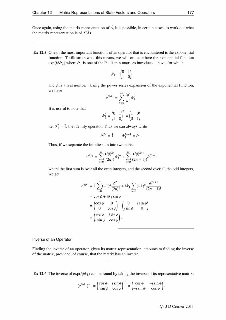
Chapter 12 Matrix Representations of State Vectors and Operators 177
Once again, using the matrix representation of A, it is possible, in certain cases, to work out whatthe matrix representation is of f (A).
Ex 12.5 One of the most important functions of an operator that is encountered is the exponentialfunction. To illustrate what this means, we will evaluate here the exponential functionexp(iφσ3) where σ1 is one of the Pauli spin matrices introduced above, for which
σ1 �
(0 11 0
)and φ is a real number. Using the power series expansion of the exponential function,we have
eiφσ1 =
∞∑n=0
iφn
n!σn
1.
It is useful to note that
σ23 �
(0 11 0
)2
=
(1 00 1
)i.e. σ2
1 = 1, the identity operator. Thus we can always write
σ2n1 = 1 σ2n+1
1 = σ1.
Thus, if we separate the infinite sum into two parts:
eiφσ1 =
∞∑n=0
(iφ)2n
(2n)!σ2n
1 +
∞∑n=0
(iφ)2n+1
(2n + 1)!σ2n+1
1
where the first sum is over all the even integers, and the second over all the odd integers,we get
eiφσ1 = 1∞∑
n=0
(−1)n φ2n
(2n)!+ iσ1
∞∑n=0
(−1)n φ2n+1
(2n + 1)!
= cos φ + iσ1 sin φ
�
(cos φ 0
0 cos φ
)+
(0 i sin φ
i sin φ 0
)=
(cos φ i sin φi sin φ cos φ
).
Inverse of an Operator
Finding the inverse of an operator, given its matrix representation, amounts to finding the inverseof the matrix, provided, of course, that the matrix has an inverse.
Ex 12.6 The inverse of exp(iφσ1) can be found by taking the inverse of its representative matrix:
(eiφσ1
)−1 �
(cos φ i sin φi sin φ cos φ
)−1
=
(cos φ −i sin φ−i sin φ cos φ
).
c© J D Cresser 2011

Chapter 12 Matrix Representations of State Vectors and Operators 178
This inverse can be recognized as being just(cos φ −i sin φ−i sin φ cos φ
)=
(cos(−φ) i sin(−φ)i sin(−φ) cos(−φ)
)which means that (
eiφσ1)−1
= e−iφσ1
a perhaps unsurprising result in that it is a particular case of the fact that the inverse ofexp(A) is just exp(−A), exactly as is the case for the exponential function of a complexvariable.
12.2.5 Eigenvectors and Eigenvalues
Operators act on states to map them into other states. Amongst the possible outcomes of the actionof an operator on a state is to map the state into a multiple of itself:
A|φ〉 = aφ|φ〉 (12.39)
where |φ〉 is, in general, a complex number. The state |φ〉 is then said to be an eigenstate or eigenketof the operator A with aφ the associated eigenvalue. The fact that operators can possess eigenstatesmight be thought of as a mathematical fact incidental to the physical content of quantum mechan-ics, but it turns out that the opposite is the case: the eigenstates and eigenvalues of various kinds ofoperators are essential parts of the physical interpretation of the quantum theory, and hence war-rant close study. Notationally, is is often useful to use the eigenvalue associated with an eigenstateto label the eigenvector, i.e. the notation
A|a〉 = a|a〉. (12.40)
This notation, or minor variations of it, will be used almost exclusively here.
Determining the eigenvalues and eigenvectors of a given operator A, occasionally referred to assolving the eigenvalue problem for the operator, amounts to finding solutions to the eigenvalueequation A|φ〉 = aφ|φ〉. Written out in terms of the matrix representations of the operator withrespect to some set of orthonormal basis vectors {|ϕ〉; n = 1, 2, . . . }, this eigenvalue equation is
A11 A12 . . .
A21 A22 . . ....
...
φ1φ2...
= a
φ1φ2...
. (12.41)
This expression is equivalent to a set of simultaneous, homogeneous, linear equations:A11 − a A12 . . .
A21 A22 − a . . ....
...
φ1φ2...
= 0 (12.42)
which have to be solved for the possible values for a, and the associated values for the componentsφ1, φ2, . . . of the eigenvectors. The procedure is standard. The determinant of coefficients mustvanish in order to get non-trivial solutions for the components φ1, φ2, . . . :∣∣∣∣∣∣∣∣∣∣
A11 − a A12 . . .
A21 A22 − a . . ....
...
∣∣∣∣∣∣∣∣∣∣ = 0 (12.43)
c© J D Cresser 2011

Chapter 12 Matrix Representations of State Vectors and Operators 179
which yields an equation known as the secular equation, or characteristic equation, that has tobe solved to give the possible values of the eigenvalues a. Once these are known, they have tobe resubstituted into Eq. (12.41) and the components φ1, φ2, . . . of the associated eigenvectorsdetermined. The details of how this is done properly belongs to a text on linear algebra and willnot be considered any further here, except to say that the eigenvectors are typically determinedup to an unknown multiplicative constant. This constant is usually fixed by the requirement thatthese eigenvectors be normalized to unity. In the case of repeated eigenvalues, i.e. when thecharacteristic polynomial has multiple roots (otherwise known as degenerate eigenvalues), thedetermination of the eigenvectors is made more complicated still. Once again, issues connectedwith these kinds of situations will not be considered here.
In general, for a state space of finite dimension, it is found that the operator A will have one ormore discrete eigenvalues a1, a2, . . . and associated eigenvectors |a1〉, |a2〉, . . . . The collection ofall the eigenvalues of an operator is called the eigenvalue spectrum of the operator. Note alsothat more than one eigenvector can have the same eigenvalue. Such an eigenvalue is said to bedegenerate.
For the present we will be confining our attention to operators that have discrete eigenvalue spectra.Modifications needed to handle continuous eigenvalues will be introduced later.
12.2.6 Hermitean Operators
Apart from certain calculational advantages, the representation of operators as matrices makes itpossible to introduce in a direct fashion Hermitean operators, already considered in a more abstractway in Section 11.3.1, which have a central role to play in the physical interpretation of quantummechanics.
To begin with, suppose we have an operator A with matrix elements Amn with respect to a set oforthonormal basis states {|ϕn〉; n = 1, 2, . . . }. From the matrix representing this operator, we canconstruct a new operator by taking the transpose and complex conjugate of the original matrix:
A11 A12 A13 . . .
A21 A22 A23 . . .
A31 A32 A33 . . ....
......
−→A∗11 A∗21 A∗31 . . .
A∗12 A∗22 A∗32 . . .
A∗13 A∗23 A∗33 . . ....
......
. (12.44)
The new matrix will represent a new operator which is obviously related to A, which we will callA†, i.e.
A† �
(A†)11 (A†)12 (A†)13 . . .
(A†)21 (A†)22 (A†)23 . . .
(A†)31 (A†)32 (A†)33 . . ....
......
=
A∗11 A∗21 A∗31 . . .
A∗12 A∗22 A∗32 . . .
A∗13 A∗23 A∗33 . . ....
......
. (12.45)
i.e.〈ϕm|A†|ϕn〉 = (〈ϕn|A|ϕm〉)∗. (12.46)
The new operator that we have created, A†, can be recognized as the Hermitean adjoint of A.The Hermitean adjoint has a useful property which we can most readily see if we use the matrixrepresentation of the operator equation
A|ψ〉 = |φ〉 (12.47)
which we earlier showed could be written as
φm =∑
n
〈ϕm|A|ϕn〉ψn. (12.48)
c© J D Cresser 2011

Chapter 12 Matrix Representations of State Vectors and Operators 180
If we now take the complex conjugate of this expression we find
φ∗m =∑
n
ψ∗n〈ϕn|A†|ϕm〉 (12.49)
which we can write in row vector form as
(φ∗1 φ∗2 . . .
)=
(ψ∗1 ψ∗2 . . .
) (A†)11 (A†)12 . . .
(A†)21 (A†)22 . . ....
...
(12.50)
which is the matrix version of〈φ| = 〈ψ|A†. (12.51)
In other words we have shown that if A|ψ〉 = |φ〉, then 〈ψ|A† = 〈φ|, a result that we used earlierto motivate the definition of the Hermitean adjoint in the first place. Thus, there are two ways toapproach this concept: either through a general abstract argument, or in terms of matrix represen-tations of an operator.
Ex 12.7 Consider the operator A which has the representation in some basis
A �
(1 i0 −1
).
Then
A† �(
1 0−i −1
).
To be noticed in this example is that A , A†.
Ex 12.8 Now consider the operator
A �
(0 −ii 0
).
Then
A† �(0 −ii 0
)i.e. A = A†.
This is an example of a situation in which A and A† are identical. In this case, the operator is saidto be selfadjoint, or Hermitean. Once again, we encountered this idea in a more general context inSection 11.4.2, where it was remarked that Hermitean operators have a number of very importantproperties which leads to their playing a central role in the physical interpretation of quantum me-chanics. These properties of Hermitean operators lead to the identification of Hermitean operatorsas representing the physically observable properties of a physical system, in a way that will bediscussed in the next Chapter.
c© J D Cresser 2011

Chapter 13
Observables and Measurements in QuantumMechanics
Till now, almost all attention has been focussed on discussing the state of a quantum system.As we have seen, this is most succinctly done by treating the package of information that
defines a state as if it were a vector in an abstract Hilbert space. Doing so provides the mathemat-ical machinery that is needed to capture the physically observed properties of quantum systems.A method by which the state space of a physical system can be set up was described in Section8.4.2 wherein an essential step was to associate a set of basis states of the system with the ex-haustive collection of results obtained when measuring some physical property, or observable, ofthe system. This linking of particular states with particular measured results provides a way thatthe observable properties of a quantum system can be described in quantum mechanics, that is interms of Hermitean operators. It is the way in which this is done that is the main subject of thisChapter.
13.1 Measurements in Quantum Mechanics
QuantumSystem S
MeasuringApparatusM
Surrounding Environment E
Figure 13.1: System S interacting withmeasuring apparatusM in the presence ofthe surrounding environment E. The out-come of the measurement is registered onthe dial on the measuring apparatus.
One of the most difficult and controversial problemsin quantum mechanics is the so-called measurementproblem. Opinions on the significance of this prob-lem vary widely. At one extreme the attitude is thatthere is in fact no problem at all, while at the otherextreme the view is that the measurement problemis one of the great unsolved puzzles of quantum me-chanics. The issue is that quantum mechanics onlyprovides probabilities for the different possible out-comes in an experiment – it provides no mechanismby which the actual, finally observed result, comesabout. Of course, probabilistic outcomes feature inmany areas of classical physics as well, but in thatcase, probability enters the picture simply becausethere is insufficient information to make a definiteprediction. In principle, that missing information isthere to be found, it is just that accessing it may be a practical impossibility. In contrast, there isno ‘missing information’ for a quantum system, what we see is all that we can get, even in prin-ciple, though there are theories that say that this missing information resides in so-called ‘hiddenvariables’. But in spite of these concerns about the measurement problem, there are some fea-tures of the measurement process that are commonly accepted as being essential parts of the finalstory. What is clear is that performing a measurement always involves a piece of equipment that
c© J D Cresser 2011

Chapter 13 Observables and Measurements in Quantum Mechanics 182
is macroscopic in size, and behaves according to the laws of classical physics. In Section 8.5, theprocess of decoherence was mentioned as playing a crucial role in giving rise to the observed clas-sical behaviour of macroscopic systems, and so it is not surprising to find that decoherence playsan important role in the formulation of most modern theories of quantum measurement. Any quan-tum measurement then appears to require three components: the system, typically a microscopicsystem, whose properties are to be measured, the measuring apparatus itself, which interacts withthe system under observation, and the environment surrounding the apparatus whose presence sup-plies the decoherence needed so that, ‘for all practical purposes (FAPP)’, the apparatus behaveslike a classical system, whose output can be, for instance, a pointer on the dial on the measuringapparatus coming to rest, pointing at the final result of the measurement, that is, a number on thedial. Of course, the apparatus could produce an electrical signal registered on an oscilloscope, orbit of data stored in a computer memory, or a flash of light seen by the experimenter as an atomstrikes a fluorescent screen, but it is often convenient to use the simple picture of a pointer.
The experimental apparatus would be designed according to what physical property it is of thequantum system that is to be measured. Thus, if the system were a single particle, the apparatuscould be designed to measure its energy, or its position, or its momentum or its spin, or some otherproperty. These measurable properties are known as observables, a concept that we have alreadyencountered in Section 8.4.1. But how do we know what it is that a particular experimental setupwould be measuring? The design would be ultimately based on classical physics principles, i.e.,if the apparatus were intended to measure the energy of a quantum system, then it would alsomeasure the energy of a classical system if a classical system were substituted for the quantumsystem. In this way, the macroscopic concepts of classical physics can be transferred to quantumsystems. We will not be examining the details of the measurement process in any great depth here.Rather, we will be more concerned with some of the general characteristics of the outputs of ameasurement procedure and how these general features can be incorporated into the mathematicalformulation of the quantum theory.
13.2 Observables and Hermitean Operators
So far we have consistently made use of the idea that if we know something definite about thestate of a physical system, say that we know the z component of the spin of a spin half particle isS z = 1
2~, then we assign to the system the state |S z = 12~〉, or, more simply, |+〉. It is at this point
that we need to look a little more closely at this idea, as it will lead us to associating an operatorwith the physical concept of an observable. Recall that an observable is, roughly speaking, anymeasurable property of a physical system: position, spin, energy, momentum . . . . Thus, we talkabout the position x of a particle as an observable for the particle, or the z component of spin, S z
as a further observable and so on.
When we say that we ‘know’ the value of some physical observable of a quantum system, weare presumably implying that some kind of measurement has been made that provided us withthis knowledge. It is furthermore assumed that in the process of acquiring this knowledge, thesystem, after the measurement has been performed, survives the measurement, and moreover ifwe were to immediately remeasure the same quantity, we would get the same result. This iscertainly the situation with the measurement of spin in a Stern-Gerlach experiment. If an atomemerges from one such set of apparatus in a beam that indicates that S z = 1
2~ for that atom,and we were to pass the atom through a second apparatus, also with its magnetic field orientedin the z direction, we would find the atom emerging in the S z = 1
2~ beam once again. Undersuch circumstances, we would be justified in saying that the atom has been prepared in the state|S z = 1
2~〉. However, the reality is that few measurements are of this kind, i.e. the system beingsubject to measurement is physically modified, if not destroyed, by the measurement process.An extreme example is a measurement designed to count the number of photons in a single mode
c© J D Cresser 2011

Chapter 13 Observables and Measurements in Quantum Mechanics 183
cavity field. Photons are typically counted by photodetectors whose mode of operation is to absorba photon and create a pulse of current. So we may well be able to count the number of photons inthe field, but in doing so, there is no field left behind after the counting is completed. All that wecan conclude, regarding the state of the cavity field, is that it is left in the vacuum state |0〉 after themeasurement is completed, but we can say nothing for certain about the state of the field beforethe measurement was undertaken. However, all is not lost. If we fiddle around with the process bywhich we put photons in the cavity in the first place, it will hopefully be the case that amongst allthe experimental procedures that could be followed, there are some that result in the cavity fieldbeing in a state for which every time we then measure the number of photons in the cavity, wealways get the result n. It is then not unreasonable to claim that the experimental procedure hasprepared the cavity field in a state which the number of photons in the cavity is n, and we canassign the state |n〉 to the cavity field.
This procedure can be equally well applied to the spin half example above. The preparationprocedure here consists of putting atoms through a Stern-Gerlach apparatus with the field orientedin the z direction, and picking out those atoms that emerge in the beam for which S z = 1
2~. Thishas the result of preparing the atom in a state for which the z component of spin would always bemeasured to have the value 1
2~. Accordingly, the state of the system is identified as |S z = 12~〉,
i.e. |+〉. In a similar way, we can associate the state |−〉 with the atom being in a state for whichthe z component of spin is always measured to be − 1
2~. We can also note that these two statesare mutually exclusive, i.e. if in the state |+〉, then the result S z = − 1
2~ is never observed, andfurthermore, we note that the two states cover all possible values for S z. Finally, the fact thatobservation of the behaviour of atomic spin show evidence of both randomness and interferencelead us to conclude that if an atom is prepared in an arbitrary initial state |S 〉, then the probabilityamplitude of finding it in some other state |S ′〉 is given by
〈S ′|S 〉 = 〈S ′|+〉〈+|S 〉 + 〈S ′|−〉〈−|S 〉
which leads, by the cancellation trick to
|S 〉 = |+〉〈+|S 〉 + |−〉〈−|S 〉
which tells us that any spin state of the atom is to be interpreted as a vector expressed as a linearcombination of the states |±〉. The states |±〉 constitute a complete set of orthonormal basis statesfor the state space of the system. We therefore have at hand just the situation that applies to theeigenstates and eigenvectors of a Hermitean operator as summarized in the following table:
Properties of a Hermitean Operator Properties of Observable S z
The eigenvalues of a Hermitean operator areall real.
Value of observable S z measured to be realnumbers ± 1
2~.Eigenvectors belonging to different eigenval-ues are orthogonal.
States |±〉 associated with different values ofthe observable are mutually exclusive.
The eigenstates form a complete set of basisstates for the state space of the system.
The states |±〉 associated with all the possiblevalues of observable S z form a complete set ofbasis states for the state space of the system.
It is therefore natural to associate with the observable S z, a Hermitean operator which we willwrite as S z such that S z has eigenstates |±〉 and associate eigenvalues ± 1
2~, i.e.
S z|±〉 = ±12~|±〉 (13.1)
c© J D Cresser 2011

Chapter 13 Observables and Measurements in Quantum Mechanics 184
so that, in the {|−〉, |+〉} basis
S z �
(〈+|S z|+〉 〈+|S z|−〉
〈−|S z|+〉 〈−|S z|−〉
)(13.2)
= 12~
(1 00 −1
). (13.3)
So, in this way, we actually construct a Hermitean operator to represent a particular measurableproperty of a physical system.
The term ‘observable’, while originally applied to the physical quantity of interest, is also appliedto the associated Hermitean operator. Thus we talk, for instance, about the observable S z. To acertain extent we have used the mathematical construct of a Hermitean operator to draw togetherin a compact fashion ideas that we have been freely using in previous Chapters.
It is useful to note the distinction between a quantum mechanical observable and the correspondingclassical quantity. The latter quantity, say the position x of a particle, represents a single possiblevalue for that observable – though it might not be known, it in principle has a definite, singlevalue at any instant in time. In contrast, a quantum observable such as S z is an operator which,through its eigenvalues, carries with it all the values that the corresponding physical quantity couldpossibly have. In a certain sense, this is a reflection of the physical state of affairs that pertainsto quantum systems, namely that when a measurement is made of a particular physical propertyof a quantum systems, the outcome can, in principle, be any of the possible values that can beassociated with the observable, even if the experiment is repeated under identical conditions.
This procedure of associating a Hermitean operator with every observable property of a quantumsystem can be readily generalized. The generalization takes a slightly different form if the ob-servable has a continuous range of possible values, such as position and momentum, as against anobservable with only discrete possible results. We will consider the discrete case first.
13.3 Observables with Discrete Values
The discussion presented in the preceding Section can be generalized into a collection of postulatesthat are intended to describe the concept of an observable. So, to begin, suppose, through anexhaustive series of measurements, we find that a particular observable, call it Q, of a physicalsystem, is found to have the values — all real numbers — q1, q2, . . . . Alternatively, we may havesound theoretical arguments that inform us as to what the possible values could be. For instance,we might be interested in the position of a particle free to move in one dimension, in which casethe observable Q is just the position of the particle, which would be expected to have any value inthe range −∞ to +∞. We now introduce the states |q1〉, |q2〉, . . . these being states for which theobservable Q definitely has the value q1, q2, . . . respectively. In other words, these are the states forwhich, if we were to measure Q, we would be guaranteed to get the results q1, q2, . . . respectively.We now have an interesting state of affairs summarized below.
1. We have an observable Q which, when measured, is found to have the values q1, q2, . . . thatare all real numbers.
2. For each possible value of Q the system can be prepared in a corresponding state |q1〉, |q2〉,. . . for which the values q1, q2, . . . will be obtained with certainty in any measurement of Q.
At this stage we are still not necessarily dealing with a quantum system. We therefore assumethat this system exhibits the properties of intrinsic randomness and interference that characterizesquantum systems, and which allows the state of the system to be identified as vectors belonging tothe state space of the system. This leads to the next property:
c© J D Cresser 2011

Chapter 13 Observables and Measurements in Quantum Mechanics 185
3. If prepared in this state |qn〉, and we measure Q, we only ever get the result qn, i.e. wenever observe the result qm with qm , qn. Thus we conclude 〈qn|qm〉 = δmn. The states{|qn〉; n = 1, 2, 3, . . .} are orthonormal.
4. The states |q1〉, |q2〉, . . . cover all the possibilities for the system and so these states form acomplete set of orthonormal basis states for the state space of the system.
That the states form a complete set of basis states means that any state |ψ〉 of the system can beexpressed as
|ψ〉 =∑
n
cn|qn〉 (13.4)
while orthonormality means that 〈qn|qm〉 = δnm from which follows cn = 〈qn|ψ〉. The completenesscondition can then be written as ∑
n
|qn〉〈qn| = 1 (13.5)
5. For the system in state |ψ〉, the probability of obtaining the result qn on measuring Q is|〈qn|ψ〉|
2 provided 〈ψ|ψ〉 = 1.
The completeness of the states |q1〉, |q2〉, . . . means that there is no state |ψ〉 of the system forwhich 〈qn|ψ〉 = 0 for every state |qn〉. In other words, we must have∑
n
|〈qn|ψ〉|2 , 0. (13.6)
Thus there is a non-zero probability for at least one of the results q1, q2, . . . to be observed – if ameasurement is made of Q, a result has to be obtained!
6. The observable Q is represented by a Hermitean operator Q whose eigenvalues are thepossible results q1, q2, . . . of a measurement of Q, and the associated eigenstates are thestates |q1〉, |q2〉, . . . , i.e. Q|qn〉 = qn|qn〉. The name ‘observable’ is often applied to theoperator Q itself.
The spectral decomposition of the observable Q is then
Q =∑
n
qn|qn〉〈qn|. (13.7)
Apart from anything else, the eigenvectors of an observable constitute a set of basis states for thestate space of the associated quantum system.
For state spaces of finite dimension, the eigenvalues of any Hermitean operator are discrete, andthe eigenvectors form a complete set of basis states. For state spaces of infinite dimension, it ispossible for a Hermitean operator not to have a complete set of eigenvectors, so that it is possiblefor a system to be in a state which cannot be represented as a linear combination of the eigenstatesof such an operator. In this case, the operator cannot be understood as being an observable as itwould appear to be the case that the system could be placed in a state for which a measurement ofthe associated observable yielded no value! To put it another way, if a Hermitean operator couldbe constructed whose eigenstates did not form a complete set, then we can rightfully claim thatsuch an operator cannot represent an observable property of the system.
It should also be pointed out that it is quite possible to construct all manner of Hermitean operatorsto be associated with any given physical system. Such operators would have all the mathematical
c© J D Cresser 2011

Chapter 13 Observables and Measurements in Quantum Mechanics 186
properties to be associated with their being Hermitean, but it is not necessarily the case that theserepresent either any readily identifiable physical feature of the system at least in part because itmight not be at all appparent how such ‘observables’ could be measured. The same is at leastpartially true classically — the quantity px2 where p is the momentum and x the position ofa particle does not immediately suggest a useful, familiar or fundamental property of a singleparticle.
13.3.1 The Von Neumann Measurement Postulate
Finally, we add a further postulate concerning the state of the system immediately after a measure-ment is made. This is the von Neumann projection postulate:
7. If on measuring Q for a system in state |ψ〉, a result qn is obtained, then the state of thesystem immediately after the measurement is |qn〉.
This postulate can be rewritten in a different way by making use of the projection operatorsintroduced in Section 11.1.3. Thus, if we write
Pn = |qn〉〈qn| (13.8)
then the state of the system after the measurement, for which the result qn was obtained, is
Pn|ψ〉√〈ψ|Pn|ψ〉
=Pn|ψ〉√|〈qn|ψ〉|2
(13.9)
where the term in the denominator is there to guarantee that the state after the measurementis normalized to unity.
This postulate is almost stating the obvious in that we name a state according to the informationthat we obtain about it as a result of a measurement. But it can also be argued that if, afterperforming a measurement that yields a particular result, we immediately repeat the measurement,it is reasonable to expect that there is a 100% chance that the same result be regained, whichtells us that the system must have been in the associated eigenstate. This was, in fact, the mainargument given by von Neumann to support this postulate. Thus, von Neumann argued that thefact that the value has a stable result upon repeated measurement indicates that the system reallyhas that value after measurement.
This postulate regarding the effects of measurement has always been a source of discussion anddisagreement. This postulate is satisfactory in that it is consistent with the manner in which theidea of an observable was introduced above, but it is not totally clear that it is a postulate thatcan be applied to all measurement processes. The kind of measurements wherein this postulateis satisfactory are those for which the system ‘survives’ the measuring process, which is certainlythe case in the Stern-Gerlach experiments considered here. But this is not at all what is usuallyencountered in practice. For instance, measuring the number of photons in an electromagneticfield inevitably involves detecting the photons by absorbing them, i.e. the photons are destroyed.Thus we may find that if n photons are absorbed, then we can say that there were n photons inthe cavity, i.e. the photon field was in state |n〉, but after the measuring process is over, it is in thestate |0〉. To cope with this fairly typical state of affairs it is necessary to generalize the notionof measurement to allow for this – so-called generalized measurement theory. But even here, itis found that the generalized measurement process being described can be understood as a vonNeumann-type projection made on a larger system of which the system of interest is a part. Thislarger system could include, for instance, the measuring apparatus itself, so that instead of makinga projective measurement on the system itself, one is made on the measuring apparatus. We willnot be discussing these aspects of measurement theory here.
c© J D Cresser 2011

Chapter 13 Observables and Measurements in Quantum Mechanics 187
13.4 The Collapse of the State Vector
The von Neumann postulate is quite clearly stating that as a consequence of a measurement, thestate of the system undergoes a discontinuous change of state, i.e. |ψ〉 → |qn〉 if the result qn isobtained on performing a measurement of an observable Q. This instantaneous change in state isknown as ‘the collapse of the state vector’. This conjures up the impression that the process ofmeasurement necessarily involves a physical interaction with the system, that moreover, results ina major physical disruption of the state of a system – one moment the system is in a state |ψ〉, thenext it is forced into a state |qn〉. However, if we return to the quantum eraser example consideredin Section 4.3.2 we see that there need not be any actual physical interaction with a system at all inorder to obtain information about it. The picture that emerges is that the change of state is nothingmore benign than being an updating, through observation, of the knowledge we have of the stateof a system as a consequence of the outcome of a measurement. While obtaining this informationmust necessarily involve some kind of physical interaction involving a measuring apparatus, thisinteraction may or may not be associated with any physical disruption to the system of interestitself. This emphasizes the notion that quantum states are as much states of knowledge as they arephysical states.
13.4.1 Sequences of measurements
Having on hand a prescription by which we can specify the state of a system after a measure-ment has been performed makes it possible to study the outcome of alternating measurements ofdifferent observables being performed on a system. We have already seen an indication of thesort of result to be found in the study of the measurement of different spin components of a spinhalf particle in Section 6.4.3. For instance, if a measurement of, say, S x is made, giving a result12~, and then S z is measured, giving, say, 1
2~, and then S x remeasured, there is an equal chancethat either of the results ± 1
2~ will be obtained, i.e. the formerly precisely known value of S x is‘randomly scrambled’ by the intervening measurement of S z. The two observables are said to beincompatible: it is not possible to have exact knowledge of both S x and S z at the same time. Thisbehaviour was presented in Section 6.4.3 as an experimentally observed fact, but we can now seehow this kind of behaviour comes about within the formalism of the theory.
If we let S x and S z be the associated Hermitean operators, we can analyze the above observedbehaviour as follows. The first measurement of S x, which yielded the outcome 1
2~, results in thespin half system ending up in the state |S x = 1
2~〉, an eigenstate of S x with eigenvalue 12~. The
second measurement, of S z, results in the system ending up in the state |S z = 12~〉, the eigenstate
of S z with eigenvalue 12~. However, this latter state cannot be an eigenstate of S x. If it were, we
would not get the observed outcome, that is, on the remeasurement of S x, we would not get arandom scatter of results (i.e. the two results S x = ±1
2~ occurring randomly but equally likely). Inthe same way we can conclude that |S x = − 1
2~〉 is also not an eigenstate of S z, and likewise, theeigenstates |S z = ± 1
2~〉 of S z cannot be eigenstates of S x. Thus we see that the two incompatibleobservables S x and S z do not share the same eigenstates.
There is a more succinct way by which to determine whether two observables are incompatible ornot. This involves making use of the concept of the commutator of two operators,
[A, B
]= AB−BA
as discussed in Section 11.1.3. To this end, consider the commutator[S x, S z
]and let it act on the
eigenstate |S z = 12~〉 = |+〉:[
S x, S z]|+〉 =
(S xS z − S zS x
)|+〉 = S x
(12~|+〉
)− S z
(S x|+〉
)=
(12~ − S z
) (S x|+〉
). (13.10)
Now let S x|+〉 = |ψ〉. Then we see that in order for this expression to vanish, we must have
S z|ψ〉 = 12~|ψ〉. (13.11)
c© J D Cresser 2011

Chapter 13 Observables and Measurements in Quantum Mechanics 188
In other words, |ψ〉 would have to be the eigenstate of S z with eigenvalue 12~, i.e. |ψ〉 ∝ |+〉, or
S x|+〉 = constant × |+〉 (13.12)
But we have just pointed out that this cannot be the case, so the expression[S x, S z
]|+〉 cannot be
zero, i.e. we must have [S x, S z
], 0. (13.13)
Thus, the operators S x and S z do not commute.
The commutator of two observables serves as a means by which it can be determined whetheror not the observables are compatible. If they do not commute, then they are incompatible: themeasurement of one of the observables will randomly scramble any preceding result known forthe other. In contrast, if they do commute, then it is possible to know precisely the value of bothobservables at the same time. An illustration of this is given later in this Chapter (Section 13.5.4),while the importance of compatibility is examined in more detail later in Chapter 14.
13.5 Examples of Discrete Valued Observables
There are many observables of importance for all manner of quantum systems. Below, some ofthe important observables for a single particle system are described. As the eigenstates of anyobservable constitutes a set of basis states for the state space of the system, these basis statescan be used to set up representations of the state vectors and operators as column vectors andmatrices. These representations are named according to the observable which defines the basisstates used. Moreover, since there are in general many observables associated with a system, thereare correspondingly many possible basis states that can be so constructed. Of course, there are aninfinite number of possible choices for the basis states of a vector space, but what this proceduredoes is pick out those basis states which are of most immediate physical significance.
The different possible representations are useful in different kinds of problems, as discussed brieflybelow. It is to be noted that the term ‘observable’ is used both to describe the physical quantitybeing measured as well as the operator itself that corresponds to the physical quantity.
13.5.1 Position of a particle (in one dimension)
The position x of a particle is a continuous quantity, with values ranging over the real numbers,and a proper treatment of such an observable raises mathematical and interpretational issues thatare dealt with elsewhere. But for the present, it is very convenient to introduce an ‘approximate’position operator via models of quantum systems in which the particle, typically an electron, canonly be found to be at certain discrete positions. The simplest example of this is the O−2 iondiscussed in Section 8.4.2.
This system can be found in two states | ± a〉, where ±a are the positions of the electron on one orthe other of the oxygen atoms. Thus these states form a pair of basis states for the state space ofthe system, which hence has a dimension 2. The position operator x of the electron is such that
x| ± a〉 = ±a| ± a〉 (13.14)
which can be written in the position representation as a matrix:
x �(〈+a|x| + a〉 〈+a|x| − a〉〈−a|x| + a〉 〈−a|x| − a〉
)=
(a 00 −a
). (13.15)
The completeness relation for these basis states reads
| + a〉〈+a| + | − a〉〈−a| = 1. (13.16)
c© J D Cresser 2011

Chapter 13 Observables and Measurements in Quantum Mechanics 189
which leads tox = a| + a〉〈+a| − a| − a〉〈−a|. (13.17)
The state space of the system has been established as having dimension 2, so any other observableof the system can be represented as a 2× 2 matrix. We can use this to construct the possible formsof other observables for this system, such as the momentum operator and the Hamiltonian.
This approach can be readily generalized to e.g. a CO−2 ion, in which case there are three possiblepositions for the electron, say x = ±a, 0 where ±a are the positions of the electron when on theoxygen atoms and 0 is the position of the electron when on the carbon atom. The position operatorx will then be such that
x| ± a〉 = ±a| ± a〉 x|0〉 = 0|0〉. (13.18)
13.5.2 Momentum of a particle (in one dimension)
As is the case of position, the momentum of a particle can have a continuous range of values,which raises certain mathematical issues that are discussed later. But we can consider the notionof momentum for our approximate position models in which the position can take only discretevalues. We do this through the observation that the matrix representing the momentum will be aN ×N matrix, where N is the dimension of the state space of the system. Thus, for the O−2 ion, themomentum operator would be represented by a two by two matrix
p �(〈+a|p| + a〉 〈+a|p| − a〉〈−a|p| + a〉 〈−a|p| − a〉
)(13.19)
though, at this stage, it is not obvious what values can be assigned to the matrix elements appearinghere. Nevertheless, we can see that, as p must be a Hermitean operator, and as this is a 2×2 matrix,p will have only 2 real eigenvalues: the momentum of the electron can be measured to have onlytwo possible values, at least within the constraints of the model we are using.
13.5.3 Energy of a Particle (in one dimension)
According to classical physics, the energy of a particle is given by
E =p2
2m+ V(x) (13.20)
where the first term on the RHS is the kinetic energy, and the second term V(x) is the potentialenergy of the particle. In quantum mechanics, it can be shown, by a procedure known as canonicalquantization, that the energy of a particle is represented by a Hermitean operator known as theHamiltonian, written H, which can be expressed as
H =p2
2m+ V(x) (13.21)
where the classical quantities p and x have been replaced by the corresponding quantum operators.The term Hamiltonian is derived from the name of the mathematician Rowan Hamilton who madeprofoundly significant contributions to the theory of mechanics. Although the Hamiltonian can beidentified here as being the total energy E, the term Hamiltonian is usually applied in mechanicsif this total energy is expressed in terms of momentum and position variables, as here, as againstsay position and velocity.
That Eq. (13.21) is ‘quantum mechanical’ is not totally apparent. Dressing the variables up asoperators by putting hats on them is not really saying that much. Perhaps most significantly there isno ~ in this expression for H, so it is not obvious how this expression can be ‘quantum mechanical’.
c© J D Cresser 2011

Chapter 13 Observables and Measurements in Quantum Mechanics 190
For instance, we have seen, at least for a particle in an infinite potential well (see Section 5.3), thatthe energies of a particle depend on ~. The quantum mechanics (and the ~) is to be found in theproperties of the operators so created that distinguish them from the classical variables that theyreplace. Specifically, the two operators x and p do not commute, in fact,
[x, p
]= i~ as shown
later, Eq. (13.133), and it is this failure to commute by an amount proportional to ~ that injects‘quantum mechanics’ into the operator associated with the energy of a particle.
As the eigenvalues of the Hamiltonian are the possible energies of the particle, the eigenvalue isusually written E and the eigenvalue equation is
H|E〉 = E|E〉. (13.22)
In the position representation, this equation becomes
〈x|H|E〉 = E〈x|E〉. (13.23)
It is shown later that, from the expression Eq. (13.21) for H, that this eigenvalue equation can bewritten as a differential equation for the wave function ψE(x) = 〈x|E〉
−~2
2md2ψE(x)
dx2 + V(x)ψE(x) = EψE(x). (13.24)
This is just the time independent Schrodinger equation.
Depending on the form of V(x), this equation will have different possible solutions, and the Hamil-tonian will have various possible eigenvalues. For instance, if V(x) = 0 for 0 < x < L and isinfinite otherwise, then we have the Hamiltonian of a particle in an infinitely deep potential well,or equivalently, a particle in a (one-dimensional) box with impenetrable walls. This problem wasdealt with in Section 5.3 using the methods of wave mechanics, where it was found that the energyof the particle was limited to the values
En =n2~2π2
2mL2 , n = 1, 2, . . . .
Thus, in this case, the Hamiltonian has discrete eigenvalues En given by Eq. (13.5.3). If we writethe associated energy eigenstates as |En〉, the eigenvalue equation is then
H|En〉 = En|En〉. (13.25)
The wave function 〈x|En〉 associated with the energy eigenstate |En〉 was also derived in Section5.3 and is given by
ψn(x) = 〈x|En〉 =
√2L
sin(nπx/L) 0 < x < L
= 0 x < 0, x > L. (13.26)
Another example is that for which V(x) = 12 kx2, i.e. the simple harmonic oscillator potential. In
this case, we find that the eigenvalues of H are
En = (n + 12 )~ω, n = 0, 1, 2, . . . (13.27)
where ω =√
k/m is the natural frequency of the oscillator. The Hamiltonian is an observableof particular importance in quantum mechanics. As will be discussed in the next Chapter, it isthe Hamiltonian which determines how a system evolves in time, i.e. the equation of motion of aquantum system is expressly written in terms of the Hamiltonian. In the position representation,this equation is just the time dependent Schrodinger equation.
c© J D Cresser 2011

Chapter 13 Observables and Measurements in Quantum Mechanics 191
The Energy Representation If the state of the particle is represented in component form withrespect to the energy eigenstates as basis states, then this is said to be the energy representation.In contrast to the position and momentum representations, the components are often discrete. Theenergy representation is useful when the system under study can be found in states with differentenergies, e.g. an atom absorbing or emitting photons, and consequently making transitions tohigher or lower energy states. The energy representation is also very important when it is theevolution in time of a system that is of interest.
13.5.4 The O−2 Ion: An Example of a Two-State System
In order to illustrate the ideas developed in the preceding sections, we will see how it is possible,firstly, how to ‘construct’ the Hamiltonian of a simple system using simple arguments, then to lookat the consequences of performing measurements of two observables for this system.
Constructing the Hamiltonian
The Hamiltonian of the ion in the position representation will be
H �
(〈+a|H| + a〉 〈+a|H| − a〉〈−a|H| + a〉 〈−a|H| − a〉
). (13.28)
Since there is perfect symmetry between the two oxygen atoms, we must conclude that the diago-nal elements of this matrix must be equal i.e.
〈+a|H| + a〉 = 〈−a|H| − a〉 = E0. (13.29)
We further know that the Hamiltonian must be Hermitean, so the off-diagonal elements are com-plex conjugates of each other. Hence we have
H �
(E0 VV∗ E0
)(13.30)
or, equivalently
H = E0| + a〉〈+a| + V | + a〉〈−a| + V∗| − a〉〈+a| + E0| − a〉〈−a|. (13.31)
Rather remarkably, we have at hand the Hamiltonian for the system with the barest of physicalinformation about the system.
In the following we shall assume V = −A and that A is a real number so that the Hamiltonianmatrix becomes
H �
(E0 −A−A E0
)(13.32)
The physical content of the results are not changed by doing this, and the results are a little easierto write down. First we can determine the eigenvalues of H by the usual method. If we writeH|E〉 = E|E〉, and put |E〉 = α| + a〉 + β| − a〉, this becomes, in matrix form(
E0 − E −A−A E0 − E
) (α
β
)= 0. (13.33)
The characteristic equation yielding the eigenvalues is then∣∣∣∣∣∣E0 − E −A−A E0 − E
∣∣∣∣∣∣ = 0. (13.34)
c© J D Cresser 2011
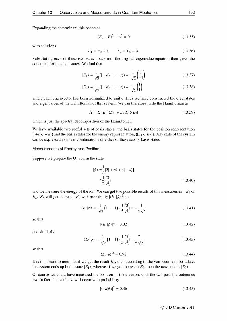
Chapter 13 Observables and Measurements in Quantum Mechanics 192
Expanding the determinant this becomes
(E0 − E)2 − A2 = 0 (13.35)
with solutionsE1 = E0 + A E2 = E0 − A. (13.36)
Substituting each of these two values back into the original eigenvalue equation then gives theequations for the eigenstates. We find that
|E1〉 =1√
2
(| + a〉 − | − a〉
)�
1√
2
(1−1
)(13.37)
|E2〉 =1√
2
(| + a〉 + | − a〉
)�
1√
2
(11
)(13.38)
where each eigenvector has been normalized to unity. Thus we have constructed the eigenstatesand eigenvalues of the Hamiltonian of this system. We can therefore write the Hamiltonian as
H = E1|E1〉〈E1| + E2|E2〉〈E2| (13.39)
which is just the spectral decomposition of the Hamiltonian.
We have available two useful sets of basis states: the basis states for the position representation{|+a〉, |−a〉} and the basis states for the energy representation, {|E1〉, |E2〉}. Any state of the systemcan be expressed as linear combinations of either of these sets of basis states.
Measurements of Energy and Position
Suppose we prepare the O−2 ion in the state
|ψ〉 =15[3| + a〉 + 4| − a〉
]�
15
(34
)(13.40)
and we measure the energy of the ion. We can get two possible results of this measurement: E1 orE2. We will get the result E1 with probability |〈E1|ψ〉|
2, i.e.
〈E1|ψ〉 =1√
2
(1 −1
)·
15
(34
)= −
1
5√
2(13.41)
so that|〈E1|ψ〉|
2 = 0.02 (13.42)
and similarly
〈E2|ψ〉 =1√
2
(1 1
)·
15
(34
)=
7
5√
2(13.43)
so that|〈E2|ψ〉|
2 = 0.98. (13.44)
It is important to note that if we get the result E1, then according to the von Neumann postulate,the system ends up in the state |E1〉, whereas if we got the result E2, then the new state is |E2〉.
Of course we could have measured the position of the electron, with the two possible outcomes±a. In fact, the result +a will occur with probability
|〈+a|ψ〉|2 = 0.36 (13.45)
c© J D Cresser 2011

Chapter 13 Observables and Measurements in Quantum Mechanics 193
and the result −a with probability|〈−a|ψ〉|2 = 0.64. (13.46)
Once again, if the outcome is +a then the state of the system after the measurement is | + a〉, andif the result −a is obtained, then the state after the measurement is | − a〉.
Finally, we can consider what happens if we were to do a sequence of measurements, first ofenergy, then position, and then energy again. Suppose the system is initially in the state |ψ〉, asabove, and the measurement of energy gives the result E1. The system is now in the state |E1〉. Ifwe now perform a measurement of the position of the electron, we can get either of the two results±a with equal probability:
|〈±a|E1〉|2 = 0.5. (13.47)
Suppose we get the result +a, so the system is now in the state | + a〉 and we remeasure theenergy. We find that now it is not guaranteed that we will regain the result E1 obtained in the firstmeasurement. In fact, we find that there is an equal chance of getting either E1 or E2:
|〈E1| + a〉|2 = |〈E2| + a〉|2 = 0.5. (13.48)
Thus we must conclude that the intervening measurement of the position of the electron has scram-bled the energy of the system. In fact, if we suppose that we get the result E2 for this second energymeasurement, thereby placing the system in the state |E2〉 and we measure the position of the elec-tron again, we find that we will get either result ±a with equal probability again! The measurementof energy and electron position for this system clearly interfere with one another. It is not pos-sible to have a precisely defined value for both the energy of the system and the position of theelectron: they are incompatible observables. We can apply the test discussed in Section 13.4.1for incompatibility of x and H here by evaluating the commutator
[x, H
]using their representative
matrices: [x, H
]=xH − H x
=a(1 00 −1
) (E0 −A−A E0
)− a
(E0 −A−A E0
) (1 00 −1
)= − 2aA
(0 11 0
), 0. (13.49)
13.5.5 Observables for a Single Mode EM Field
A somewhat different example from those presented above is that of the field inside a single modecavity (see pp 132, 150). In this case, the basis states of the electromagnetic field are the numberstates {|n〉, n = 0, 1, 2, . . .} where the state |n〉 is the state of the field in which there are n photonspresent.
Number Operator From the annihilation operator a (Eq. (11.57)) and creation operator a† (Eq.(11.72)) for this field, defined such that
a|n〉 =√
n|n − 1〉, a|0〉 = 0
a†|n〉 =√
n + 1|n + 1〉
we can construct a Hermitean operator N defined by
N = a†a (13.50)
which can be readily shown to be such that
N |n〉 = n|n〉. (13.51)
c© J D Cresser 2011
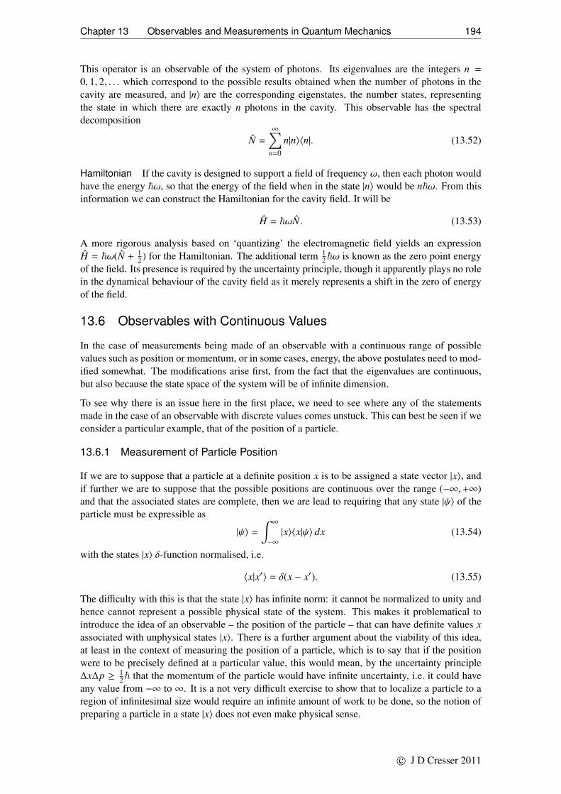
Chapter 13 Observables and Measurements in Quantum Mechanics 194
This operator is an observable of the system of photons. Its eigenvalues are the integers n =
0, 1, 2, . . . which correspond to the possible results obtained when the number of photons in thecavity are measured, and |n〉 are the corresponding eigenstates, the number states, representingthe state in which there are exactly n photons in the cavity. This observable has the spectraldecomposition
N =
∞∑n=0
n|n〉〈n|. (13.52)
Hamiltonian If the cavity is designed to support a field of frequency ω, then each photon wouldhave the energy ~ω, so that the energy of the field when in the state |n〉 would be n~ω. From thisinformation we can construct the Hamiltonian for the cavity field. It will be
H = ~ωN. (13.53)
A more rigorous analysis based on ‘quantizing’ the electromagnetic field yields an expressionH = ~ω(N + 1
2 ) for the Hamiltonian. The additional term 12~ω is known as the zero point energy
of the field. Its presence is required by the uncertainty principle, though it apparently plays no rolein the dynamical behaviour of the cavity field as it merely represents a shift in the zero of energyof the field.
13.6 Observables with Continuous Values
In the case of measurements being made of an observable with a continuous range of possiblevalues such as position or momentum, or in some cases, energy, the above postulates need to mod-ified somewhat. The modifications arise first, from the fact that the eigenvalues are continuous,but also because the state space of the system will be of infinite dimension.
To see why there is an issue here in the first place, we need to see where any of the statementsmade in the case of an observable with discrete values comes unstuck. This can best be seen if weconsider a particular example, that of the position of a particle.
13.6.1 Measurement of Particle Position
If we are to suppose that a particle at a definite position x is to be assigned a state vector |x〉, andif further we are to suppose that the possible positions are continuous over the range (−∞,+∞)and that the associated states are complete, then we are lead to requiring that any state |ψ〉 of theparticle must be expressible as
|ψ〉 =
∫ ∞
−∞
|x〉〈x|ψ〉 dx (13.54)
with the states |x〉 δ-function normalised, i.e.
〈x|x′〉 = δ(x − x′). (13.55)
The difficulty with this is that the state |x〉 has infinite norm: it cannot be normalized to unity andhence cannot represent a possible physical state of the system. This makes it problematical tointroduce the idea of an observable – the position of the particle – that can have definite values xassociated with unphysical states |x〉. There is a further argument about the viability of this idea,at least in the context of measuring the position of a particle, which is to say that if the positionwere to be precisely defined at a particular value, this would mean, by the uncertainty principle∆x∆p ≥ 1
2~ that the momentum of the particle would have infinite uncertainty, i.e. it could haveany value from −∞ to ∞. It is a not very difficult exercise to show that to localize a particle to aregion of infinitesimal size would require an infinite amount of work to be done, so the notion ofpreparing a particle in a state |x〉 does not even make physical sense.
c© J D Cresser 2011

Chapter 13 Observables and Measurements in Quantum Mechanics 195
The resolution of this impasse involves recognizing that the measurement of the position of aparticle is, in practice, only ever done to within the accuracy, δx say, of the measuring apparatus.In other words, rather than measuring the precise position of a particle, what is measured is itsposition as lying somewhere in a range (x − 1
2δx, x + 12δx). We can accommodate this situation
within the theory by defining a new set of states that takes this into account. This could be donein a number of ways, but the simplest is to suppose we divide the continuous range of values of xinto intervals of length δx, so that the nth segment is the interval ((n − 1)δx, nδx) and let xn be apoint within the nth interval. This could be any point within this interval but it is simplest to takeit to be the midpoint of the interval, i.e. xn = (n− 1
2 )δx. We then say that the particle is in the state|xn〉 if the measuring apparatus indicates that the position of the particle is in the nth segment.
In this manner we have replaced the continuous case by the discrete case, and we can now proceedalong the lines of what was presented in the preceding Section. Thus we can introduce an observ-able xδx that can be measured to have the values {xn; n = 0,±1,±2 . . .}, with |xn〉 being the state ofthe particle for which xδx has the value xn. We can then construct a Hermitean operator xδx witheigenvalues {xn; n = 0,±1,±2 . . .} and associated eigenvectors {|xn〉; n = 0,±1,±2, . . .} such that
xδx|xn〉 = xn|xn〉. (13.56)
The states {|xn; n = 0,±1,±2, . . .〉} will form a complete set of orthonormal basis states for theparticle, so that any state of the particle can be written
|ψ〉 =∑
n
|xn〉〈xn|ψ〉 (13.57)
with 〈xn|xm〉 = δnm. The observable xδx would then be given by
xδx =∑
n
xn|xn〉〈xn|. (13.58)
Finally, if a measurement of xδx is made and the result xn is observed, then the immediate post-measurement state of the particle will be
Pn|ψ〉√〈ψ|Pn|ψ〉
(13.59)
where Pn is the projection operatorPn = |xn〉〈xn|. (13.60)
To relate all this back to the continuous case, it is then necessary to take the limit, in some sense,of δx → 0. This limiting process has already been discussed in Section 10.2.2, in an equivalentbut slightly different model of the continuous limit. The essential points will be repeated here.
Returning to Eq. (13.57), we can define a new, unnormalized state vector |xn〉 by
|xn〉 =|xn〉√δx
(13.61)
The states |xn〉 continue to be eigenstates of xδx, i.e.
xδx |xn〉 = xn |xn〉 (13.62)
as the factor 1/√δx merely renormalizes the length of the vectors. Thus these states |xn〉 continue
to represent the same physical state of affairs as the normalized state, namely that when in thisstate, the particle is in the interval (xn −
12δx, xn + 1
2δx).
c© J D Cresser 2011

Chapter 13 Observables and Measurements in Quantum Mechanics 196
In terms of these unnormalized states, Eq. (13.57) becomes
|ψ〉 =∑
n
|xn〉 〈xn|ψ〉δx. (13.63)
If we let δx→ 0, then, in this limit the sum in Eq. (13.63) will define an integral with respect to x:
|ψ〉 =
∫ ∞
−∞
|x〉〈x|ψ〉 dx (13.64)
where we have introduced the symbol |x〉 to represent the δx→ 0 limit of |xn〉 i.e.
|x〉 = limδx→0
|xn〉√δx. (13.65)
This then is the idealized state of the particle for which its position is specified to within a van-ishingly small interval around x as δx approaches zero. From Eq. (13.64) we can extract thecompleteness relation for these states ∫ ∞
−∞
|x〉〈x| dx = 1. (13.66)
This is done at a cost, of course. By the same arguments as presented in Section 10.2.2, the newstates |x〉 are δ-function normalized, i.e.
〈x|x′〉 = δ(x − x′) (13.67)
and, in particular, are of infinite norm, that is, they cannot be normalized to unity and so do notrepresent physical states of the particle.
Having introduced these idealized states, we can investigate some of their further properties anduses. The first and probably the most important is that it gives us the means to write down theprobability of finding a particle in any small region in space. Thus, provided the state |ψ〉 isnormalized to unity, Eq. (13.64) leads to
〈ψ|ψ〉 = 1 =
∫ ∞
−∞
|〈x|ψ〉|2 dx (13.68)
which can be interpreted as saying that the total probability of finding the particle somewhere inspace is unity. More particularly, we also conclude that |〈x|ψ〉|2 dx is the probability of finding theposition of the particle to be in the range (x, x + dx).
If we now turn to Eq. (13.58) and rewrite it in terms of the unnormalized states we have
xδx =∑
n
xn |xn〉 〈xn|δx (13.69)
so that in a similar way to the derivation of Eq. (13.64) this gives, in the limit of δx → 0, the newoperator x, i.e.
x =
∫ ∞
−∞
x|x〉〈x| dx. (13.70)
This then leads to the δx→ 0 limit of the eigenvalue equation for xδx, Eq. (13.62) i.e.
x|x〉 = x|x〉 (13.71)
a result that also follows from Eq. (13.70) on using the δ-function normalization condition. Thisoperator x therefore has as eigenstates the complete set of δ-function normalized states {|x〉;−∞ <
c© J D Cresser 2011

Chapter 13 Observables and Measurements in Quantum Mechanics 197
x < ∞} with associated eigenvalues x and can be looked on as being the observable correspondingto an idealized, precise measurement of the position of a particle.
While these states |x〉 can be considered idealized limits of the normalizable states |xn〉 it mustalways be borne in mind that these are not physically realizable states – they are not normalizable,and hence are not vectors in the state space of the system. They are best looked on as a convenientfiction with which to describe idealized situations, and under most circumstances these states canbe used in much the same way as discrete eigenstates. Indeed it is one of the benefits of theDirac notation that a common mathematical language can be used to cover both the discrete andcontinuous cases. But situations can and do arise in which the cavalier use of these states can leadto incorrect or paradoxical results. We will not be considering such cases here.
The final point to be considered is the projection postulate. We could, of course, idealize thisby saying that if a result x is obtained on measuring x, then the state of the system after themeasurement is |x〉. But given that the best we can do in practice is to measure the position of theparticle to within the accuracy of the measuring apparatus, we cannot really go beyond the discretecase prescription given in Eq. (13.59) except to express it in terms of the idealized basis states |x〉.So, if the particle is in some state |ψ〉, we can recognize that the probability of getting a result xwith an accuracy of δx will be given by
∫ x+12 δx
x− 12 δx|〈x′|ψ〉|2dx′ =
∫ x+12 δx
x− 12 δx〈ψ|x′〉〈x′|ψ〉dx′
= 〈ψ|
[ ∫ x+12 δx
x− 12 δx|x′〉〈x′|dx′
]|ψ〉 = 〈ψ|P(x, δx)|ψ〉 (13.72)
where we have introduced an operator P(x, δx) defined by
P(x, δx) =
∫ x+12 δx
x− 12 δx|x′〉〈x′|dx′. (13.73)
We can readily show that this operator is in fact a projection operator since
[P(x, δx)
]2=
∫ x+12 δx
x−12 δx
dx′∫ x+
12 δx
x− 12 δx
dx′′|x′〉〈x′|x′′〉〈x′′|
=
∫ x+12 δx
x−12 δx
dx′∫ x+
12 δx
x− 12 δx
dx′′|x′〉δ(x′ − x′′)〈x′′|
=
∫ x+12 δx
x−12 δx
dx′|x′〉〈x′|
=P(x, δx). (13.74)
This suggests, by comparison with the corresponding postulate in the case of discrete eigenval-ues, that if the particle is initially in the state |ψ〉, then the state of the particle immediately aftermeasurement be given by
P(x, δx)|ψ〉√〈ψ|P(x, δx)|ψ〉
=
∫ x+12 δx
x−12 δx|x′〉〈x′|ψ〉dx′√∫ x+
12 δx
x− 12 δx|〈x′|ψ〉|2dx′
(13.75)
c© J D Cresser 2011

Chapter 13 Observables and Measurements in Quantum Mechanics 198
It is this state that is taken to be the state of the particle immediately after the measurement hasbeen performed, with the result x being obtained to within an accuracy δx.
Further development of these ideas is best done in the language of generalized measurementswhere the projection operator is replaced by an operator that more realistically represents theoutcome of the measurement process. We will not be pursuing this any further here.
At this point, we can take the ideas developed for the particular case of the measurement of positionand generalize them to apply to the measurement of any observable quantity with a continuousrange of possible values. The way in which this is done is presented in the following Section.
13.6.2 General Postulates for Continuous Valued Observables
Suppose we have an observable Q of a system that is found, for instance through an exhaustiveseries of measurements, to have a continuous range of values θ1 < q < θ2. In practice, it is notthe observable Q that is measured, but rather a discretized version in which Q is measured to anaccuracy δq determined by the measuring device. If we represent by |q〉 the idealized state of thesystem in the limit δq→ 0, for which the observable definitely has the value q, then we claim thefollowing:
1. The states {|q〉; θ1 < q < θ2} form a complete set of δ-function normalized basis states forthe state space of the system.
That the states form a complete set of basis states means that any state |ψ〉 of the system can beexpressed as
|ψ〉 =
∫ θ2
θ1
c(q)|q〉 (13.76)
while δ-function normalized means that 〈q|q′〉 = δ(q− q′) from which follows c(q) = 〈q|ψ〉 so that
|ψ〉 =
∫ θ2
θ1
|q〉〈q|ψ〉 dq. (13.77)
The completeness condition can then be written as∫ θ2
θ1
|q〉〈q| dq = 1 (13.78)
2. For the system in state |ψ〉, the probability of obtaining the result q lying in the range (q, q +
dq) on measuring Q is |〈q|ψ〉|2dq provided 〈ψ|ψ〉 = 1.
Completeness means that for any state |ψ〉 it must be the case that∫ θ2
θ1
|〈q|ψ〉|2dq , 0 (13.79)
i.e. there must be a non-zero probability to get some result on measuring Q.
3. The observable Q is represented by a Hermitean operator Q whose eigenvalues are thepossible results {q; θ1 < q < θ2}, of a measurement of Q, and the associated eigenstates arethe states {|q〉; θ1 < q < θ2}, i.e. Q|q〉 = q|q〉. The name ‘observable’ is often applied to theoperator Q itself.
c© J D Cresser 2011

Chapter 13 Observables and Measurements in Quantum Mechanics 199
The spectral decomposition of the observable Q is then
Q =
∫ θ2
θ1
q|q〉〈q| dq. (13.80)
As in the discrete case, the eigenvectors of an observable constitute a set of basis states for thestate space of the associated quantum system.
A more subtle difficulty is now encountered if we turn to the von Neumann postulate concerningthe state of the system after a measurement is made. If we were to transfer the discrete statepostulate directly to the continuous case, we would be looking at proposing that obtaining theresult q in a measurement of Q would mean that the state after the measurement is |q〉. This is astate that is not permitted as it cannot be normalized to unity. Thus we need to take account of theway a measurement is carried out in practice when considering the state of the system after themeasurement. Following on from the particular case of position measurement presented above, wewill suppose that Q is measured with a device of accuracy δq. This leads to the following generalstatement of the von Neumann measurement postulate for continuous eigenvalues:
4. If on performing a measurement of Q with an accuracy δq, the result is obtained in the range(q − 1
2δq, q + 12δq), then the system will end up in the state
P(q, δq)|ψ〉√〈ψ|P(q, δq)|ψ〉
(13.81)
where
P(q, δq) =
∫ q+12 δq
q− 12 δq|q′〉〈q′|dq′. (13.82)
Even though there exists this precise statement of the projection postulate for continuous eigen-values, it is nevertheless a convenient fiction to assume that the measurement of an observable Qwith a continuous set of eigenvalues will yield one of the results q with the system ending up inthe state |q〉 immediately afterwards. While this is, strictly speaking, not really correct, it can beused as a convenient shorthand for the more precise statement given above.
As mentioned earlier, further development of these ideas is best done in the language of general-ized measurements.
13.7 Examples of Continuous Valued Observables
13.7.1 Position and momentum of a particle (in one dimension)
These two observables are those which are most commonly encountered in wave mechanics. Inthe case of position, we are already able to say a considerable amount about the properties of thisobservable. Some further development is required in order to be able to deal with momentum.
Position observable (in one dimension)
In one dimension, the position x of a particle can range over the values −∞ < x < ∞. Thus theHermitean operator x corresponding to this observable will have eigenstates |x〉 and associatedeigenvalues x such that
x|x〉 = x|x〉, −∞ < x < ∞. (13.83)
c© J D Cresser 2011

Chapter 13 Observables and Measurements in Quantum Mechanics 200
As the eigenvalues cover a continuous range of values, the completeness relation will be expressedas an integral:
|ψ〉 =
∫ ∞
−∞
|x〉〈x|ψ〉 (13.84)
where 〈x|ψ〉 = ψ(x) is the wave function associated with the particle. Since there is a continuouslyinfinite number of basis states |x〉, these states are delta-function normalized:
〈x|x′〉 = δ(x − x′). (13.85)
The operator itself can be expressed as
x =
∫ ∞
−∞
x|x〉〈x| dx. (13.86)
The Position Representation The wave function is, of course, just the components of the statevector |ψ〉 with respect to the position eigenstates as basis vectors. Hence, the wave function isoften referred to as being the state of the system in the position representation. The probabilityamplitude 〈x|ψ〉 is just the wave function, written ψ(x) and is such that |ψ(x)|2dx is the probabilityof the particle being observed to have a momentum in the range x to x + dx.
The one big difference here as compared to the discussion in Chapter 12 is that the basis vectorshere are continuous, rather than discrete, so that the representation of the state vector is not asimple column vector with discrete entries, but rather a function of the continuous variable x.Likewise, the operator x will not be represented by a matrix with discrete entries labelled, forinstance, by pairs of integers, but rather it will be a function of two continuous variables:
〈x|x|x′〉 = xδ(x − x′). (13.87)
The position representation is used in quantum mechanical problems where it is the position of theparticle in space that is of primary interest. For instance, when trying to determine the chemicalproperties of atoms and molecules, it is important to know how the electrons in each atom tendto distribute themselves in space in the various kinds of orbitals as this will play an importantrole in determining the kinds of chemical bonds that will form. For this reason, the positionrepresentation, or the wave function, is the preferred choice of representation. When working inthe position representation, the wave function for the particle is found by solving the Schrodingerequation for the particle.
Momentum of a particle (in one dimension)
As for position, the momentum p is an observable which can have any value in the range −∞ <
p < ∞ (this is non-relativistic momentum). Thus the Hermitean operator p will have eigenstates|p〉 and associated eigenvalues p:
p|p〉 = p|p〉, −∞ < p < ∞. (13.88)
As the eigenvalues cover a continuous range of values, the completeness relation will also beexpressed as an integral:
|ψ〉 =
∫ +∞
−∞
|p〉〈p|ψ〉 dp (13.89)
where the basis states are delta-function normalized:
〈p|p′〉 = δ(p − p′). (13.90)
The operator itself can be expressed as
p =
∫ +∞
−∞
p|p〉〈p| dp. (13.91)
c© J D Cresser 2011

Chapter 13 Observables and Measurements in Quantum Mechanics 201
Momentum Representation If the state vector is represented in component form with respect tothe momentum eigenstates as basis vectors, then this is said to be the momentum representation.The probability amplitude 〈p|ψ〉 is sometimes referred to as the momentum wave function, writtenψ(p) and is such that |ψ(p)|2dp is the probability of the particle being observed to have a momen-tum in the range p to p + dp. It turns out that the momentum wave function and the position wavefunction are Fourier transform pairs, a result that is shown below.
The momentum representation is preferred in problems in which it is not so much where a particlemight be in space that is of interest, but rather how fast it is going and in what direction. Thus, themomentum representation is often to be found when dealing with scattering problems in whicha particle of well defined momentum is directed towards a scattering centre, e.g. an atomic nu-cleus, and the direction in which the particle is scattered, and the momentum and/or energy of thescattered particle are measured, though even here, the position representation is used more oftenthan not as it provides a mental image of the scattering process as waves scattering off an obstacle.Finally, we can also add that there is an equation for the momentum representation wave functionwhich is equivalent to the Schrodinger equation.
Properties of the Momentum Operator
The momentum operator can be introduced into quantum mechanics by a general approach basedon the space displacement operator. But at this stage it is nevertheless possible to draw someconclusions about the properties of the momentum operator based on the de Broglie hypothesisconcerning the wave function of a particle of precisely known momentum p and energy E.
The momentum operator in the position representation From the de Broglie relation and Ein-stein’s formula, the wave function Ψ(x, t) to be associated with a particle of momentum p andenergy E will have a wave number k and angular frequency ω given by p = ~k and E = ~ω. Wecan then guess what this wave function would look like:
Ψ(x, t) = 〈x|Ψ(t)〉 = Aei(kx−ωt) + Be−i(kx−ωt) + Cei(kx+ωt) + De−i(kx+ωt). (13.92)
The expectation is that the wave will travel in the same direction as the particle, i.e. if p > 0, thenthe wave should travel in the direction of positive x. Thus we must reject those terms with theargument (kx + ωt) and so we are left with
〈x|Ψ(t)〉 = Aei(px/~−ωt) + Be−i(px/~−ωt) (13.93)
where we have substituted for k in terms of p. The claim then is that the state |Ψ(t)〉 is a statefor which the particle definitely has momentum p, and hence it must be an eigenstate of themomentum operator p, i.e.
p|Ψ(t)〉 = p|Ψ(t)〉 (13.94)
which becomes, in the position representation
〈x|p|Ψ(t)〉 =p〈x|Ψ(t)〉
=p(Aei(px/~−ωt) + Be−i(px/~−ωt)
).
(13.95)
The only simple way of obtaining the factor p is by taking the derivative of the wave function withrespect to x, though this does not immediately give us what we want, i.e.
〈x|p|Ψ(t)〉 = −i~∂
∂x
(Aei(px/~−ωt) − Be−i(px/~−ωt)
), p〈x|Ψ(t)〉 (13.96)
which tells us that the state |Ψ(t)〉 is not an eigenstate of p, at least if we proceed along the lines ofintroducing the derivative with respect to x. However, all is not lost. If we choose one or the otherof the two terms in the expression for 〈x|Ψ(t)〉 e.g.
〈x|Ψ(t)〉 = Aei(px/~−ωt) (13.97)
c© J D Cresser 2011

Chapter 13 Observables and Measurements in Quantum Mechanics 202
we find that〈x|p|Ψ(t)〉 = −i~
∂
∂x〈x|Ψ(t)〉 = p〈x|Ψ(t)〉 (13.98)
as required. This suggests that we have arrived at a candidate for the wave function for a particleof definite momentum p. But we could have chosen the other term with coefficient B. However,this other choice amounts to reversing our choice of the direction of positive x and positive t —its exponent can be written i(p(−x)/~ − ω(−t)). This is itself a convention, so we can in fact useeither possibility as the required momentum wave function without affecting the physics. To be inkeeping with the convention that is usually adopted, the choice Eq. (13.97) is made here.
Thus, by this process of elimination, we have arrived at an expression for the wave function of aparticle with definite momentum p. Moreover, we have extracted an expression for the momentumoperator p in that, if |p〉 is an eigenstate of p, then, in the position representation
〈x|p|p〉 = −i~ddx〈x|p〉. (13.99)
This is a result that can be readily generalized to apply to any state of the particle. By makinguse of the fact that the momentum eigenstate form a complete set of basis states, we can write anystate |ψ〉 as
|ψ〉 =
∫ +∞
−∞
|p〉〈p|ψ〉 dp (13.100)
so that
〈x|p|ψ〉 =
∫ +∞
−∞
〈x|p|p〉〈p|ψ〉 dp
= − i~ddx
∫ +∞
−∞
〈x|p〉〈p|ψ〉 dp
= − i~ddx〈x|ψ〉
or〈x|p|ψ〉 = −i~
ddxψ(x). (13.101)
From this result it is straightforward to show that
〈x|pn|ψ〉 = (−i~)n dn
dxnψ(x). (13.102)
For instance,〈x|p2|ψ〉 = 〈x|p|φ〉 (13.103)
where |φ〉 = p|ψ〉. Thus
〈x|p2|ψ〉 = −i~ddxφ(x). (13.104)
Butφ(x) = 〈x|φ〉 = 〈x|p|ψ〉 = −i~
ddxψ(x). (13.105)
Using this and Eq. (13.104), we get
〈x|p2|ψ〉 = −i~ddx
(−i~
ddx
)ψ(x) = −~2 d2
dx2ψ(x) (13.106)
In general we see that, when working in the position representation, the substitution
p −→ −i~ddx
(13.107)
c© J D Cresser 2011

Chapter 13 Observables and Measurements in Quantum Mechanics 203
can consistently be made. This is an exceedingly important result that plays a central role in wavemechanics, in particular in setting up the Schrodinger equation for the wave function.
One final result can be established using this correspondence. Consider the action of the operator
D(a) = eipa/~ (13.108)
on an arbitrary state |ψ〉 i.e.|φ〉 = D(a)|ψ〉 (13.109)
which becomes, in the position representation
〈x|φ〉 = φ(x) = 〈x|D(a)|ψ〉. (13.110)
Expanding the exponential and making the replacement Eq. (13.107) we have
D(a) = 1+ ipa/~+ (ia/~)2 12!
p2 + (ia/~)3 13!
p3 + . . . −→ 1+addx
+a2
2!d2
dx2 +a3
3!d3
dx3 + . . . (13.111)
we get
φ(x) =
(1 + a
ddx
+a2
2!d2
dx2 +a3
3!d3
dx3 + . . .
)ψ(x)
=ψ(x) + aψ′(x) +a2
2!ψ′′(x) +
a3
3!ψ′′′(x) + . . .
=ψ(x + a)
(13.112)
where the series appearing above is recognized as the Maclaurin series expansion about x = a.Thus we see that the state |φ〉 obtained by the action of the operator D(a) on |ψ〉 is to diplace thewave function a distance a along the x axis. This result illustrates the deep connection betweenmomentum and displacement in space, a relationship that is turned on its head in Chapter 16 wheremomentum is defined in terms of the displacement operator.
The normalized momentum eigenfunction Returning to the differential equation Eq. (13.99),we can readily obtain the solution
〈x|p〉 = Aeipx/~ (13.113)
where A is a coefficient to be determined by requiring that the states |p〉 be delta function normal-ized. Note that our wave function Eq. (13.97) gives the time development of the eigenfunction〈x|p〉, Eq. (13.113).
The normalization condition is that
〈p|p′〉 = δ(p − p′) (13.114)
which can be written, on using the completeness relation for the position eigenstates
δ(p − p′) =
∫ +∞
−∞
〈p|x〉〈x|p′〉 dx
=|A|2∫ +∞
−∞
e−i(p−p′)x/~ dp
=|A|22π~δ(p − p′)
(13.115)
where we have used the representation of the Dirac delta function given in Section 10.2.3. Thuswe conclude
|A|2 =1
2π~. (13.116)
c© J D Cresser 2011

Chapter 13 Observables and Measurements in Quantum Mechanics 204
It then follows that〈x|p〉 =
1√
2π~eipx/~. (13.117)
This result can be used to relate the wave function for a particle in the momentum and positionrepresentations. Using the completeness of the momentum states we can write for any state |ψ〉 ofthe particle
|ψ〉 =
∫ +∞
−∞
|p〉〈p|ψ〉 dp (13.118)
which becomes, in the position representation
〈x|ψ〉 =
∫ +∞
−∞
〈x|p〉〈p|ψ〉 dp (13.119)
or, in terms of the wave functions:
ψ(x) =1√
2π~
∫ +∞
−∞
eipx/~ψ(p) dp (13.120)
which immediately shows that the momentum and position representation wave functions areFourier transform pairs. It is a straightforward procedure to then show that
ψ(p) =1√
2π~
∫ +∞
−∞
e−ipx/~ψ(x) dx (13.121)
either by simply inverting the Fourier transform, or by expanding the state vector |ψ〉 in terms ofthe position eigenstates.
That the position and momentum wave functions are related in this way has a very important con-sequence that follows from a fundamental property of Fourier transform pairs. Roughly speaking,there is an inverse relationship between the width of a function and its Fourier transformed com-panion. This is most easily seen if suppose, somewhat unrealistically, that ψ(x) is of the form
ψ(x) =
1√
a|x| ≤ 1
2 a
0 |x| > 12 a
(13.122)
The full width of ψ(x) is a. The momentum wave function is
ψ(p) =
√2~π
sin(pa/~)p
. (13.123)
An estimate of the width of ψ(p) is given by determining the positions of the first zeroes of ψ(p)on either side of the central maximum at p = 0, that is at p = ±π~/a. The separation of thesetwo zeroes, 2π~/a, is an overestimate of the width of the peak so we take this width to be halfthis separation, thus giving an estimate of π~/a. Given that the square of the wave functions i.e.|ψ(x)|2 and |ψ(p)|2 give the probability distribution for position and momentum respectively, it isclearly the case that the wider the spread in the possible values of the position of the particle, i.e.the larger a is made, there is a narrowing of the spread in the range of values of momentum, andvice versa. This inverse relationship is just the Heisenberg uncertainty relation reappearing, and ismore fully quantified in terms of the uncertainties in position and momentum defined in Chapter14.
c© J D Cresser 2011

Chapter 13 Observables and Measurements in Quantum Mechanics 205
Position momentum commutation relation The final calculation in here is to determine thecommutator [x, p] = x p − px of the two operators x and p. This can be done most readily in theposition representation. Thus we will consider
〈x|[x, p]|ψ〉 = 〈x|(x p − px)|ψ〉 (13.124)
where |ψ〉 is an arbitrary state of the particle. This becomes, on using the fact that the state 〈x| isan eigenstate of x with eigenvalue x
〈x|[x, p]|ψ〉 = x〈x|p|ψ〉 − 〈x|p|ξ〉 (13.125)
where |ξ〉 = x|ψ〉. Expressed in terms of the differential operator, this becomes
〈x|[x, p]|ψ〉 = −i~(x
ddxψ(x) −
ddxξ(x)
). (13.126)
Butξ(x) = 〈x|ξ〉 = 〈x|x|ψ〉 = x〈x|ψ〉 = xψ(x) (13.127)
so thatddxξ(x) = x
ddxψ(x) + ψ(x). (13.128)
Combining this altogether then gives
〈x|[x, p]|ψ〉 = i~ψ(x) = i~〈x|ψ〉. (13.129)
The completeness of the position eigenstates can be used to write this as∫ +∞
−∞
|x〉〈x|[x, p]|ψ〉 = i~∫ +∞
−∞
|x〉〈x|ψ〉 (13.130)
or[x, p]|ψ〉 = i~1|ψ〉. (13.131)
Since the state |ψ〉 is arbitrary, we can conclude that
[x, p] = i~1 (13.132)
though the unit operator on the right hand side is usually understood, so the relation is written
[x, p] = i~. (13.133)
This is perhaps the most important result in non-relativistic quantum mechanics as it embodiesmuch of what makes quantum mechanics ‘different’ from classical mechanics. For instance, if theposition and momentum operators were classical quantities, then the commutator would vanish,or to put it another way, it is that fact that ~ , 0 that gives us quantum mechanics. It turns out that,amongst other things, the fact that the commutator does not vanish implies that it is not possibleto have precise information on the position and the momentum of a particle, i.e. position andmomentum are incompatible observables.
13.7.2 Field operators for a single mode cavity
A physical meaning can be given to the annihilation and creation operators defined above in termsof observables of the field inside the cavity. This done here in a non-rigorous way, relying ona trick by which we relate the classical and quantum ways of specifying the energy of the field.We have earlier arrived at an expression for the quantum Hamiltonian of the cavity field as givenin Eq. (13.53), i.e. H = ~ωa†a, which as we have already pointed out, is missing the zero-point
c© J D Cresser 2011

Chapter 13 Observables and Measurements in Quantum Mechanics 206
contribution 12~ω that is found in a full quantum theory of the electromagnetic field. However,
assuming we had never heard of this quantum theory, then we could proceed by comparing thequantum expression we have derived with the classical expression for the energy of the singlemode EM field inside the cavity.
A little more detail about the single mode field is required before the classical Hamiltonian can beobtained. This field will be assumed to be a plane polarized standing wave confined between twomirrors of areaA, separated by a distance L in the z direction. Variation of the field in the x and ydirections will also be ignored, so the total energy of the field will be given by
H = 12
∫V
(ε0E2(z, t) + B2(z, t)/µ0
)dxdydz (13.134)
where the classical electric field is E(z, t) = Re[E(t)] sin(ωz/c), i.e. of complex amplitude E(t) =
Ee−iωt, the magnetic field is B(z, t) = c−1Im[E(t)] cos(ωz/c), and whereV = AL is the volume ofthe cavity.
The integral can be readily carried out to give
H = 14ε0E
∗EV (13.135)
We want to establish a correspondence between the two expressions for the Hamiltonian, i.e.
~ωa†a←→ 14ε0E
∗EV
in order to give some sort of physical interpretation of a, apart from its interpretation as a photonannihilation operator. We can do this by reorganizing the various terms so that the correspondencelooks like 2e−iφ
√~ωVε0
a†2eiφ
√~ωVε0
a
←→ E∗Ewhere exp(iφ) is an arbitrary phase factor, i.e. it could be chosen to have any value and the cor-respondence would still hold. A common choice is to take this phase factor to be i. The mostobvious next step is to identify an operator E closely related to the classical quantity E by
E = 2i
√~ωVε0
a
so that we get the correspondence E†E ←→ E∗E.
We can note that the operator E is still not Hermitean, but recall that the classical electric field wasobtained from the real part of E, so that we can define a Hermitean electric field operator by
E(z) = 12[E + E†
]sin(ωz/c) = i
√~ωVε0
[a − a†
]sin(ωz/c)
to complete the picture. In this way we have identified a new observable for the field inside thecavity, the electric field operator. This operator is, in fact, an example of a quantum field operator.Of course, the derivation presented here is far from rigorous. That this operator is indeed theelectric field operator can be shown to follow from the full analysis as given by the quantumtheory of the electromagnetic field.
In the same way, an expression for the magnetic field operator can be determined from the expres-sion for the classical magnetic field, with the result:
B(z) =
√µ0~ωV
(a + a†) cos(ωz/c). (13.136)
c© J D Cresser 2011

Chapter 13 Observables and Measurements in Quantum Mechanics 207
The above are two new observables for the system so it is natural to ask what is their eigenvaluespectrum. We can get at this in an indirect fashion by examining the properties of the two Her-mitean operators i(a − a†) and a + a†. For later purposes, it is convenient to rescale these twooperators and define
X =
√~
2ω(a + a†) and P = −i
√~ω2
(a − a†). (13.137)
As the choice of notation implies, the aim is to show that these new operators are, mathematicallyat least, closely related to the position and momentum operators x and p for a single particle. Thedistinctive quantum feature of these latter operators is their commutation relation, so the aim isto evaluate the commutator of X and P. To do so, we need to know the value of the commutator[a, a†]. We can determine this by evaluating [a, a†]|n〉where |n〉 is an arbitrary number state. Usingthe properties of the annihilation and creation operators a and a† given by
a|n〉 =√
n|n − 1〉 and a†|n〉 =√
n + 1|n + 1〉
we see that[a, a†]|n〉 = aa†|n〉 − a†a|n〉
= a√
n + 1|n + 1〉 − a†√
n|n − 1〉
= (n + 1)|n〉 − n|n〉
= |n〉
from which we conclude[a, a†] = 1. (13.138)
If we now make use of this result when evaluating [X, P] we find
[X, P] = −i 12~[a + a†, a − a†] = i~ (13.139)
where use has been made of the properties of the commutator as given in Eq. (11.24).
In other words, the operators X and P obey exactly the same commutation relation as position andmomentum for a single particle, x and p respectively. This is of course a mathematical correspon-dence i.e. there is no massive particle ‘behind the scenes’ here, but the mathematical correspon-dence is one that is found to arise in the formulation of the quantum theory of the electromagneticfield. But what it means to us here is that the two observables X and P will, to all intents andpurposes have the same properties as x and p. In particular, the eigenvalues of X and P will becontinuous, ranging from −∞ to +∞. Since we can write the electric field operator as
E(z) = −
√2Vε0
P sin(ωz/c) (13.140)
we conclude that the electric field operator will also have a continuous range of eigenvalues from−∞ to +∞. This is in contrast to the number operator or the Hamiltonian which both have adiscrete range of values. A similar conclusion applies for the magnetic field, which can be writtenin terms of X:
B(z) = ω
√2µ0
VX cos(ωz/c). (13.141)
What remains is to check the form of the Hamiltonian of the field as found directly from theexpressions for the electric and magnetic field operators. This can be calculated via the quantumversion of the classical expression for the field energy, Eq. (13.134), i.e.
H = 12
∫V
[ε0E2(z) + B2(z)/µ0
]dxdydz. (13.142)
c© J D Cresser 2011
Chapter 13 Observables and Measurements in Quantum Mechanics 208
Substituting for the field operators and carrying out the spatial integrals gives
= 14~ω
[−(a − a†)2 + (a + a†)2
](13.143)
= 12~ω
[aa† + a†a
]. (13.144)
Using the commutation rule[a, a†
]= 1 we can write this as
H = ~ω(a†a + 1
2
). (13.145)
Thus, we recover the original expression for the Hamiltonian, but now with the additional zero-point energy contribution 1
2~ω. That we do not recover the assumed starting point for the Hamilto-nian is an indicator that the above derivation is not entirely rigorous. Nevertheless, it does achievea useful purpose in that we have available expressions for the electric and magnetic field operators,and the Hamiltonian, for the a single mode electromagnetic field.
c© J D Cresser 2011

Chapter 14
Probability, Expectation Value and Uncertainty
We have seen that the physically observable properties of a quantum system are representedby Hermitean operators (also referred to as ‘observables’) such that the eigenvalues of
the operator represents all the possible results that could be obtained if the associated physicalobservable were to be measured. The eigenstates of the operator are the states of the systemfor which the associated eigenvalue would be, with 100% certainty, the measured result, if theobservable were measured. If the system were in any other state then the possible outcomes ofthe measurement cannot be predicted precisely – different possible results could be obtained, eachone being an eigenvalue of the associated observable, but only the probabilities can be determinedof these possible results. This physically observed state-of-affairs is reflected in the mathematicalstructure of quantum mechanics in that the eigenstates of the observable form a complete set ofbasis states for the state space of the system, and the components of the state of the system withrespect to this set of basis states gives the probability amplitudes, and by squaring, the probabilitiesof the various outcomes being observed.
Given the probabilistic nature of the measurement outcomes, familiar tools used to analyze statis-tical data such as the mean value and standard deviation play a natural role in characterizing theresults of such measurements. The expectation or mean value of an observable is a concept takenmore or less directly from the classical theory of probability and statistics. Roughly speaking, itrepresents the (probability-weighted) average value of the results of many repetitions of the mea-surement of an observable, with each measurement carried out on one of very many identicallyprepared copies of the same system. The standard deviation of these results is then a measure ofthe spread of the results around the mean value and is known, in a quantum mechanical context,as the uncertainty.
14.1 Observables with Discrete Values
The probability interpretation of quantum mechanics plays a central, in fact a defining, role inquantum mechanics, but the precise meaning of this probability interpretation has as yet not beenfully spelt out. However, for the purposes of defining the expectation value and the uncertainty itis necessary to look a little more closely at how this probability is operationally defined. The waythis is done depends on whether the observable has a discrete or continuous set of eigenvalues, soeach case is discussed separately. We begin here with the discrete case.
14.1.1 Probability
If A is an observable for a system with a discrete set of values {a1, a2, . . .}, then this observableis represented by a Hermitean operator A that has these discrete values as its eigenvalues, andassociated eigenstates {|an〉, n = 1, 2, 3, . . .} satisfying the eigenvalue equation A|an〉 = an|an〉.
c© J D Cresser 2011

Chapter 14 Probability, Expectation Value and Uncertainty 210
These eigenstates form a complete, orthonormal set so that any state |ψ〉 of the system can bewritten
|ψ〉 =∑
n
|an〉〈an|ψ〉
where, provided 〈ψ|ψ〉 = 1, then
|〈an|ψ〉|2 = probability of obtaining the result an on mea-
suring A.
To see what this means in an operational sense, we can suppose that we prepare N identical copiesof the system all in exactly the same fashion so that each copy is presumably in the same state |ψ〉.This set of identical copies is sometimes called an ensemble. If we then perform a measurementof A for each member of the ensemble, i.e. for each copy, we find that we get randomly varyingresults e.g.
Copy: 1 2 3 4 5 6 7 8 . . . NResult: a5 a3 a1 a9 a3 a8 a5 a9 . . . a7
Now count up the number of times we get the result a1 – call this N1, and similarly for the numberof times N2 we get the result a2 and so on. Then
Nn
N= fraction of times the result an is obtained. (14.1)
What we are therefore saying is that if the experiment is performed on an increasingly large num-ber of identical copies, i.e. as N → ∞, then we find that
limN→∞
Nn
N= |〈an|ψ〉|
2. (14.2)
This is the so-called ‘frequency’ interpretation of probability in quantum mechanics, i.e. the prob-ability predicted by quantum mechanics gives us the frequency with which an outcome will occurin the limit of a very large number of repetitions of an experiment.
There is another interpretation of this probability, more akin to ‘betting odds’ in the sense thatin application, it is usually the case that the experiment is a ‘one-off’ affair, i.e. it is not possibleto repeat the experiment many times over under identical conditions. It then makes more senseto try to understand this probability as a measure of the likelihood of a particular result beingactually observed, in the same way that betting odds for a horse to win a race is a measure of theconfidence there is in the horse actually winning. After all, a race is only run once, so while it ispossible to imagine the race being run many times over under identical conditions, and that theodds would provide a measure of how many of these imagined races a particular horse would win,there appears to be some doubt of the practical value of this line of thinking. Nevertheless, the‘probability as frequency’ interpretation of quantum probabilities is the interpretation that is stillmost commonly to be found in quantum mechanics.
14.1.2 Expectation Value
We can now use this result to arrive at an expression for the average or mean value of all theseresults. If the measurement is repeated N times, the average will be
N1
Na1 +
N2
Na2 + . . . =
∑n
Nn
Nan. (14.3)
c© J D Cresser 2011
Chapter 14 Probability, Expectation Value and Uncertainty 211
Now take the limit of this result for N → ∞, and call the result 〈A〉:
〈A〉 = limN→∞
∑n
Nn
Nan =
∑n
|〈an|ψ〉|2an. (14.4)
It is a simple matter to use the properties of the eigenstates of A to reduce this expression to acompact form:
〈A〉 =∑
n
〈ψ|an〉〈an|ψ〉an
=∑
n
〈ψ|A|an〉〈an|ψ〉
= 〈ψ|A{∑
n
|an〉〈an|
}|ψ〉
= 〈ψ|A|ψ〉 (14.5)
where the completeness relation for the eigenstates of A has been used.
This result can be readily generalized to calculate the expectation values of any function of theobservable A. Thus, in general, we have that
〈 f (A)〉 =∑
n
|〈an|ψ〉|2 f (an) = 〈ψ| f (A)|ψ〉 (14.6)
a result that will find immediate use below when the uncertainty of an observable will be consid-ered.
While the expectation value has been defined in terms of the outcomes of measurements of anobservable, the same concept of an ‘expectation value’ is applied to non-Hermitean operatorswhich do not represent observable properties of a system. Thus if A is not Hermitean and hencenot an observable we cannot make use of the idea of a collection of results of experiments overwhich an average is taken to arrive at an expectation value. Nevertheless, we continue to make useof the notion of the expectation value 〈A〉 = 〈ψ|A|ψ〉 even when A is not an observable.
14.1.3 Uncertainty
The uncertainty of the observable A is a measure of the spread of results around the mean 〈A〉. Itis defined in the usual way, that is the difference between each measured result and the mean iscalculated, i.e. an−〈A〉, then the average taken of the square of all these differences. In the limit ofN → ∞ repetitions of the same experiment we arrive at an expression for the uncertainty (∆A)2:
(∆A)2 = limN→∞
∑n
Nn
N(an − 〈A〉)2 =
∑n
|〈an|ψ〉|2(an − 〈A〉)2. (14.7)
As was the case for the expectation value, this can be written in a more compact form:
(∆A)2 =∑
n
〈ψ|an〉〈an|ψ〉(an − 〈A〉)2
=∑
n
〈ψ|an〉〈an|ψ〉(a2n − 2an〈A〉 + 〈A〉2)
=∑
n
〈ψ|an〉〈an|ψ〉a2n − 2〈A〉
∑n
〈ψ|an〉〈an|ψ〉an + 〈A〉2∑
n
〈ψ|an〉〈an|ψ〉
c© J D Cresser 2011
Chapter 14 Probability, Expectation Value and Uncertainty 212
Using f (A)|an〉 = f (an)|an〉 then gives
(∆A)2 =∑
n
〈ψ|A2|an〉〈an|ψ〉 − 2〈A〉∑
n
〈ψ|A|an〉〈an|ψ〉 + 〈A〉2〈ψ|{∑
n
|an〉〈an|
}|ψ〉
= 〈ψ|A2{∑
n
|an〉〈an|
}|ψ〉 − 2〈A〉〈ψ|A
{∑n
|an〉〈an|
}|ψ〉 + 〈A〉2〈ψ|ψ〉
Assuming that the state |ψ〉 is normalized to unity, and making further use of the completenessrelation for the basis states |an〉 this becomes
(∆A)2 = 〈ψ|A2|ψ〉 − 2〈A〉2 + 〈A〉2 = 〈A2〉 − 〈A〉2. (14.8)
We can get another useful expression for the uncertainty if we proceed in a slightly differentfashion:
(∆A)2 =∑
n
〈ψ|an〉〈an|ψ〉(an − 〈A〉)2
=∑
n
〈ψ|an〉(an − 〈A〉)2〈an|ψ〉
Now using f (A)|an〉 = f (an)|an〉 then gives
(∆A)2 =∑
n
〈ψ|(A − 〈A〉)2|an〉〈an|ψ〉
= 〈ψ|(A − 〈A〉)2{∑
n
|an〉〈an|
}|ψ〉
= 〈ψ|(A − 〈A〉)2|ψ〉
= 〈(A − 〈A〉)2〉. (14.9)
Thus we have, for the uncertainty ∆A, the two results
(∆A)2 = 〈(A − 〈A〉)2〉 = 〈A2〉 − 〈A〉2. (14.10)
Just as was the case for the expectation value, we can also make use of this expression to formallycalculate the uncertainty of some operator A even if it is not an observable, though the fact that theresults cannot be interpreted as the standard deviation of a set of actually observed results meansthat the physical interpretation of the uncertainty so obtained is not particularly clear.
Ex 14.1 For the O−2 ion (see p 117) calculate the expectation value and standard deviation of theposition of the electron if the ion is prepared in the state |ψ〉 = α| + a〉 + β| − a〉.
In this case, the position operator is given by
x = a| + a〉〈+a| − a| − a〉〈−a|
so thatx|ψ〉 = aα| + a〉 − aβ| − a〉
and hence the expectation value of the position of the electron is
〈ψ|x|ψ〉 = 〈x〉 = a(|α|2 − |β|2
)
c© J D Cresser 2011
Chapter 14 Probability, Expectation Value and Uncertainty 213
which can be recognized as being just
〈x〉 = (+a) × probability |α|2 of measuring electron position to be +a
+ (−a) × probability |β|2 of measuring electron position to be −a.
In particular, if the probability of the electron being found on either oxygen atom isequal, that is |α|2 = |β|2 = 1
2 , then the expectation value of the position of the electron is〈x〉 = 0.
The uncertainty in the position of the electron is given by
(∆x)2 = 〈x2〉 − 〈x〉2.
We already have 〈x〉, and to calculate 〈x2〉 it is sufficient to make use of the expressionabove for x|ψ〉 to give
x2|ψ〉 = x[aα| + a〉 − aβ| − a〉
]= a2[α| + a〉 + β| − a〉
]= a2|ψ〉
so that 〈ψ|x2|ψ〉 = 〈x2〉 = a2. Consequently, we find that
(∆x)2 = a2 − a2(|α|2 − |β|2)2
= a2[1 −
(|α|2 − |β|2
)2]
= a2(1 − |α|2 + |β|2)(
1 + |α|2 − |β|2)
Using 〈ψ|ψ〉 = |α|2 + |β|2 = 1 this becomes
(∆x)2 = 4a2|α|2|β|2
from which we find that∆x = 2a|αβ|.
This result is particularly illuminating in the case of |α|2 = |β|2 = 12 where we find that
∆x = a. This is the symmetrical situation in which the mean position of the electronis 〈x〉 = 0, and the uncertainty is exactly equal to the displacement of the two oxygenatoms on either side of this mean.
Ex 14.2 As an example of an instance in which it is useful to deal with the expectation valuesof non-Hermitean operators, we can turn to the system consisting of identical photonsin a single mode cavity (see pp 132, 150, 193). If the cavity field is prepared in thenumber state |n〉, an eigenstate of the number operator N defined in Eq. (13.50), then weimmediately have 〈N〉 = n and ∆N = 0.
However, if we consider a state such as |ψ〉 = (|n〉 + |n + 1〉)/√
2 we find that
〈N〉 = 12 (〈n| + 〈n + 1|)N(|n〉 + |n + 1〉)
= 12 (〈n| + 〈n + 1|)(n|n〉 + (n + 1)|n + 1〉)
= n + 12 .
while
(∆N)2 = 〈N2〉 − 〈N〉2
= 12 (〈n| + 〈n + 1|)N N(|n〉 + |n + 1〉) − (n + 1
2 )2
= 12 (n〈n| + (n + 1)〈n + 1|)(n|n〉 + (n + 1)|n + 1〉) − (n + 1
2 )2
= 12 (n2 + (n + 1)2) − (n + 1
2 )2
= 14 .
c© J D Cresser 2011

Chapter 14 Probability, Expectation Value and Uncertainty 214
Not unexpectedly,we find that the uncertainty in the photon number is now non-zero.
We can also evaluate the expectation value of the annihilation operator a, Eq. (11.57) forthe system in each of the above states. Thus, for the number state |n〉 we have
〈a〉 = 〈n|a|n〉 =√
n〈n|n − 1〉 = 0
while for the state |ψ〉 = (|n〉 + |n + 1〉)/√
2 we find that
〈a〉 = 12
√n + 1.
It is an interesting exercise to try to give some kind of meaning to these expectationvalues for a, particularly since the expectation value of a non-Hermitean operator doesnot, in general, represent the average of a collection of results obtained when measuringsome observable. The meaning is provided via the demonstration in Section 13.5.5 that ais directly related to the electric field strength inside the cavity. From that demonstration,it can be seen that the imaginary part of 〈a〉 is to be understood as being proportional tothe average strength of the electric (or magnetic) field inside the cavity, i.e. Im〈a〉 ∝ 〈E〉where E is the electric field operator. We can then interpret the expressions obtainedabove for the expectation value of the field as saying little more than that for the field inthe number state |n〉, the electric field has an average value of zero. However, this is notto say that the field is not overall zero. Thus, we can calculate the uncertainty in the fieldstrength ∆E. This entails calculating
∆E =
√〈n|E2|n〉 − 〈n|E|n〉2 =
√〈n|E2|n〉.
Using the expression
E = i
√~ω
2Vε0
[a − a†
]we see that
〈n|E2|n〉 =~ω
2Vε0〈n|aa† + a†a|n〉
where the other contributions, 〈n|aa|n〉 = 〈n|a†a†|n〉 = 0. It then follows from the prop-erties of the creation and annihilation operators that
〈n|E2|n〉 =~ω
2Vε0(2n + 1)
and hence
∆E =
√~ω
2Vε0
√(2n + 1).
So, while the field has an expectation value of zero, it has non-zero fluctuations aboutthis mean. In fact, if the cavity contains no photons (n = 0), we see that even then thereis a random electric field present:
∆E =
√~ω
2Vε0.
This non-vanishing electric random electric field is known as the vacuum field fluctua-tions, and its presence shows that even the quantum vacuum is alive with energy!
c© J D Cresser 2011

Chapter 14 Probability, Expectation Value and Uncertainty 215
14.2 Observables with Continuous Values
Much of what has been said in the preceding Section carries through with relatively minor changesin the case in which the observable under consideration has a continuous eigenvalue spectrum.However, rather than discussing the general case, we will consider only the particular instance ofthe measurement of the position represented by the position operator x of a particle.
14.2.1 Probability
Recall from Section 13.6.1, p 194, that in order to measure the position – an observable with acontinuous range of possible values – it was necessary to suppose that the measuring apparatushad a finite resolution δx in which case we divide the continuous range of values of x into intervalsof length δx, so that the nth segment is the interval ((n − 1)δx, nδx). If we let xn be the point inthe middle of the nth interval, i.e. xn = (n − 1
2 )δx, we then say that the particle is in the state|xn〉 if the measuring apparatus indicates that the position of the particle is in the nth segment.The observable being measured is now represented by the Hermitean operator xδx with discreteeigenvalues {xn; n = 0,±1,±2 . . .} and associated eigenvectors {|xn〉; n = 0,±1,±2, . . .} such thatxδx|xn〉 = xn|xn〉.
0
5
10
15
20
25
30
35
40
45
50
6543210-1-2-3-4-5
1
P(x) = |〈x|ψ〉|2Nn
Nδx
n
Figure 14.1: Histogram of the frequencies of detectionsin each interval ((n − 1)δx, nδx), n = 0,±1,±2, . . . for themeasurement of the position of a particle for N identicalcopies all prepared in the state |ψ〉 and using apparatus withresolution δx. Also plotted is the probability distribution|〈x|ψ〉|2 expected in the limit of N → ∞ and δx→ 0.
We can now imagine setting up, as inthe discrete case discussed above, anensemble of N identical systems allprepared in the state |ψ〉, and the po-sition of the particle measured with aresolution δx. We then take note ofthe number of times Nn in which theparticle was observed to lie in the nth
interval and from this data constructa histogram of the frequency Nn/N ofthe results for each interval. An ex-ample of such a set of results is illus-trated in Fig. 14.1.
As was discussed earlier, the claim isnow made that for N large, the fre-quency with which the particle is ob-served to lie in the nth interval ((n −1)δx, nδx), that is Nn/N, should ap-proximate to the probability predicted by quantum mechanics, i.e.
Nn
N≈ |〈x|ψ〉|2δx (14.11)
or, in other wordsNn
Nδx≈ |〈x|ψ〉|2. (14.12)
Thus, a histogram of the frequency Nn/N normalized per unit δx should approximate to the ide-alized result |〈x|ψ〉|2 expected in the limit of N → ∞. This is also illustrated in Fig. 14.1. In thelimit of the resolution δx→ 0, the tops of the histograms would approach the smooth curve in Fig.14.1. All this amounts to saying that
limδx→0
(lim
N→∞
Nn
Nδx
)= |〈x|ψ〉|2. (14.13)
The generalization of this result to other observables with continuous eigenvalues is essentiallyalong the same lines as presented above for the position observable.
c© J D Cresser 2011

Chapter 14 Probability, Expectation Value and Uncertainty 216
14.2.2 Expectation Values
We can now calculate the expectation value of an observable with continuous eigenvalues bymaking use of the limiting procedure introduced above. Rather than confining our attention tothe particular case of particle position, we will work through the derivation of the expression forthe expectation value of an arbitrary observable with a continuous eigenvalue spectrum. Thus,suppose we are measuring an observable A with a continuous range of eigenvalues α1 < a < α2.We do this, as indicated in the preceding Section by supposing that the range of possible values isdivided up into small segments of length δa. Suppose the measurement is repeated N times on Nidentical copies of the same system, all prepared in the same state |ψ〉. In general, the same resultwill not be obtained every time, so suppose that on Nn occasions, a result an was obtained whichlay in the nth interval ((n − 1)δa, nδa). The average of all these results will then be
N1
Na1 +
N2
Na2 + . . . . (14.14)
If we now take the limit of this result for N → ∞, then we can replace the ratios Nn/N by|〈an|ψ〉|
2δa to give
|〈a1|ψ〉|2a1δa + |〈a2|ψ〉|
2a2δa + |〈a3|ψ〉|2a3δa + . . . =
∑n
|〈an|ψ〉|2anδa. (14.15)
Finally, if we let δa→ 0 the sum becomes an integral. Calling the result 〈A〉, we get:
〈A〉 =
∫ α2
α1
|〈a|ψ〉|2ada. (14.16)
It is a simple matter to use the properties of the eigenstates of A to reduce this expression to acompact form:
〈A〉 =
∫ α2
α1
〈ψ|a〉a〈a|ψ〉da
=
∫ α2
α1
〈ψ|A|a〉〈a|ψ〉da
= 〈ψ|A{∫ α2
α1
|a〉〈a|da}|ψ〉
= 〈ψ|A|ψ〉 (14.17)
where the completeness relation for the eigenstates of A has been used. This is the same compactexpression that was obtained in the discrete case earlier.
In the particular case in which the observable is the position of a particle, then the expectationvalue of position will be given by
〈x〉 =
∫ +∞
−∞
|〈x|ψ〉|2x dx =
∫ +∞
−∞
|ψ(x)|2x dx (14.18)
Also, as in the discrete case, this result can be readily generalized to calculate the expectationvalues of any function of the observable A. Thus, in general, we have that
〈 f (A)〉 =
∫ α2
α1
|〈a|ψ〉|2 f (a) da = 〈ψ| f (A)|ψ〉 (14.19)
a result that will find immediate use below when the uncertainty of an observable with continuouseigenvalues will be considered.
Once again, as in the discrete case, if A is not Hermitean and hence not an observable we cannotmake use of the idea of a collection of results of experiments over which an average is takento arrive at an expectation value. Nevertheless, we continue to make use of the notion of theexpectation value as defined by 〈A〉 = 〈ψ|A|ψ〉 even when A is not an observable.
c© J D Cresser 2011
Chapter 14 Probability, Expectation Value and Uncertainty 217
14.2.3 Uncertainty
We saw in the preceding subsection how the expectation value of an observabel with a continuousrange of possible values can be obtained by first ‘discretizing’ the data, then making use of theideas developed in the discrete case to set up the expectation value, and finally taking appropriatelimits. The standard deviation or uncertainty in the outcomes of a collection of measurements ofa continuously valued observable can be calculated in essentially the same fashion – after all it isnothing but another kind of expectation value, and not surprisingly, the same formal expressionis obtained for the uncertainty. Thus, if A is an observable with a continuous range of possibleeigenvalues α1 < a < α2, then the uncertainty ∆A is given by 〈(A − 〈A〉)2〉
(∆A)2 = 〈(A − 〈A〉)2〉 = 〈A2〉 − 〈A〉2 (14.20)
where
〈A2〉 =
∫ α2
α1
a2|〈a|ψ〉|2 da and 〈A〉 =
∫ α2
α1
a|〈a|ψ〉|2 da (14.21)
In particular, the uncertainty in the position of a particle would be given by ∆x where
(∆x)2 = 〈x2〉 − 〈x〉2 =
∫ +∞
−∞
x2|ψ(x)|2 dx −(∫ +∞
−∞
x|ψ(x)|2 dx)2
. (14.22)
Ex 14.3 In the case of a particle trapped in the region 0 < x < L by infinitely high potential bar-riers – i.e. the particle is trapped in an infinitely deep potential well – the wave functionfor the energy eigenstates are given by
ψn(x) =
√
2L
sin(nπx/L) 0 < x < L
0 x < 0 x > L
The integrals are straightforward (see Eq. (5.39)) and yield
∆x =L
2nπ
√n2π2 − 6
3
which approaches, for n→ ∞
∆x→L
2√
3which is the result that would be expected for a particle that was equally likely to befound anywhere within the potential well.
14.3 The Heisenberg Uncertainty Relation
14.4 Compatible and Incompatible Observables
In all the discussion so far regarding measurement of observables of a system, we have confinedour attention to considering one observable only at a time. However, it is clear that physicalsystems will in general possess a number of observable properties.
14.4.1 Degeneracy
c© J D Cresser 2011

Chapter 15
Time Evolution in Quantum Mechanics
Physical systems are, in general, dynamical, i.e. they evolve in time. The dynamics of classicalmechanical systems are described by Newton’s laws of motion, while the dynamics of the
classical electromagnetic field is determined by Maxwell’s equations. Either Newton’s equationsor Maxwell’s equations constitute laws of physics whose form is particular to the kind of systemthat is being described, though some unification is provided in terms of Hamilton’s principle, auniversal way of stating the laws of classical dynamics. What we require is a means by which thedynamical properties of quantum systems can be described, i.e. given the state |ψ(0)〉 of a quantumsystem at some initial time t = 0, what is required is a physical law that tells us what the state willbe at some other time t, i.e. a quantum law of evolution. Given that a state vector is a repositoryof the information known about a system, what is required is a general physical law that tells ushow this information evolves in time in response to the particular physical circumstances that thesystem of interest finds itself in. It is to be expected that the details of this law will vary fromsystem to system, but it turns out that the law of evolution can be written in a way that holds truefor all physical systems, in some sense similar to the way that Hamilton’s principle provides a wayof stating classical dynamical laws in one compact form. Of course, the quantum law of evolutionis Schrodinger’s equation.
15.1 Stationary States
The idea of ‘stationary states’ was first introduced by Bohr as a name given to those states ofa hydrogen atom for which the orbits that the electron occupied were stable, i.e. the electronremained in the same orbital state for all time, in contrast to the classical physics prediction thatno orbiting electron could remain in orbit forever: it would always radiate away its energy andspiral into the proton. Although Bohr’s original concept is now no longer appropriate, the notionof a stationary state remains a valid one. It is a term that is now used to identify those states ofa quantum system that do not change in time. This is not to say that a stationary state is one forwhich ‘nothing happens’ – there is still a rich collection of dynamical physics to be associated withsuch a state – but a stationary state turns out to be one for which the probabilities of outcomes ofa measurement of any property of the system is the same no matter at what time the measurementis made. Our aim initial aim here is to try to learn what properties the state vector representing astationary state might have.
The starting point is to let |ψ(0)〉 be the initial state of the system, and |ψ(t)〉 be the state at someother time t. As this state vector at time t is supposed to represent the system in the same physicalstate, the most that these two states can differ by is a multiplicative factor, u(t) say, i.e.
|ψ(t)〉 = u(t)|ψ(0)〉. (15.1)
c© J D Cresser 2011

Chapter 15 Time Evolution in Quantum Mechanics 219
Since we would expect that if the initial state |ψ(0)〉 is normalized to unity, then so would the state|ψ(t)〉, we can write
〈ψ(t)|ψ(t)〉 = |u(t)|2〈ψ(0)|ψ(0)〉 (15.2)
and hence|u(t)|2 = 1 (15.3)
so we must conclude thatu(t) = e−iφ(t) (15.4)
where φ(t) is an as yet unknown time dependent phase. Thus we can write
|ψ(t)〉 = e−iφ(t)|ψ(0)〉. (15.5)
This result is very general, and perhaps not all that surprising, but it becomes more revealing if wefocus on an important special case, that in which the system is assumed to be isolated i.e. that ithas no interaction with any other system – the dynamics of the system are determined solely byits own internal interactions. What this means is that if, for such a system, we were initially toprepare the system in some state and allow it to evolve for, say, ten minutes, it should not matterwhen this ‘initial’ time might be. If we start the experiment at noon and allow it to run for tenminutes, or if we started it at midnight and allow it to run for ten minutes, the state of the systemafter the ten minutes has elapsed should be the same in either case, simply because the system isisolated: the way it behaves cannot be affected by anything external. In contrast, if the systemwere open, i.e. not isolated, then there is the prospect of time dependent external influences actingon the system – e.g. an externally produced laser pulse fired at an atom – so the evolution of thestate of the atom would differ depending on the starting time. In such a situation the system mightnot have any stationary states at all as it is always potentially being forced to change because ofthese external influences.
What all this amounts to as that, for an isolated system, we can chose the initial time to be anyarbitrary time t0, and the evolution of |ψ(t0)〉 up to the time t would be given by
|ψ(t)〉 = e−iφ(t−t0)|ψ(t0)〉 (15.6)
i.e. what matters is how long the system evolves for, not what we choose as our starting time.
If we now consider the evolution of the system in a stationary state over a time interval (t, t′), thenwe have
|ψ(t′)〉 = e−iφ(t′−t)|ψ(t)〉 = e−iφ(t′−t)e−iφ(t−t0)|ψ(t0)〉 (15.7)
but over the interval (t0, t′) we have
|ψ(t′)〉 = e−iφ(t′−t0)|ψ(0)〉 (15.8)
so by comparing the last two equations we find that
e−iφ(t′−t0) = e−iφ(t′−t)e−iφ(t−t0) (15.9)
orφ(t − t0) = φ(t′ − t) + φ(t − t0), (15.10)
an equation for φ with the solutionφ(t) = ωt (15.11)
where ω is a constant. Thus we can conclude that
|ψ(t)〉 = e−iωt|ψ(0)〉 (15.12)
which is the required expression for the evolution in time of a stationary state of an isolated system.
c© J D Cresser 2011

Chapter 15 Time Evolution in Quantum Mechanics 220
15.2 The Schrodinger Equation – a ‘Derivation’.
The expression Eq. (15.12) involves a quantity ω, a real number with the units of (time)−1, i.e. ithas the units of angular frequency. In order to determine the physical meaning to be given to thisquantity, we can consider this expression in the particular case of a free particle of energy E andmomentum p, for which the wave function is given by
Ψ(x, t) = Aeikxe−iωt (15.13)
where, according to the de Broglie-Bohr relations, E = ~ω and p = ~k. In this case, we see that ωis directly related to the energy of the particle. This is a relationship that we will assume appliesto any physical system, so that we will rewrite Eq. (15.12) as
|ψ(t)〉 = e−iEt/~|ψ(0)〉 (15.14)
and further identify the stationary state |ψ(0)〉 as being an eigenstate of the energy observable Hfor the system, otherwise known as the Hamiltonian.
We now make an inductive leap, and identify a stationary state of any physical system as being aneigenstate of the Hamiltonian of the system, with the associated eigenvalue being the energy to beassociated with the stationary state.
|E(t)〉 = e−iEt/~|E〉 (15.15)
withH|E〉 = E|E〉 (15.16)
from which we getH|E(t)〉 = E|E(t)〉. (15.17)
If we differentiate Eq. (15.15) we find
i~d|E(t)〉
dt= E|E(t)〉 = H|E(t)〉 (15.18)
which we can now use to obtain the equation satisfied by an arbitrary state vector |ψ(t)〉. First,since the eigenstates of H, call them {|E1〉, |E2〉, . . . , |EN〉}, form a complete set of basis states, wecan write for the initial state
|ψ(0)〉 =
N∑n=1
|En〉〈En|ψ(0)〉. (15.19)
The time evolved version is then
|ψ(t)〉 =
N∑n=1
e−iEnt/~|En〉〈En|ψ(0)〉 (15.20)
which, on differentiating, becomes
i~d|ψ(t)〉
dt=i~
N∑n=1
Ene−iEnt/~|En〉〈En|ψ(t)〉
=
N∑n=1
He−iEnt/~|En〉〈En|ψ(t)〉
=HN∑
n=1
e−iEnt/~|En〉〈En|ψ(t)〉
=H|ψ(t)〉 (15.21)
c© J D Cresser 2011

Chapter 15 Time Evolution in Quantum Mechanics 221
so we haveH|ψ(t)〉 = i~
d|ψ(t)〉dt
(15.22)
which is the celebrated Schrodinger equation in vector form.
Determining the solution of this equation is the essential task in determining the dynamical prop-erties of a quantum system. If the eigenvectors and eigenvalues of the Hamiltonian can be readilydetermined, the solution can be written down directly, i.e. it is just
|ψ(t)〉 =∑
n
e−iEnt/~|En〉〈En|ψ(0)〉. (15.23)
However, it is not necessary to follow this procedure, at least explicitly, as there are in generalmany ways to solving the equations. In any case, the process of obtaining the eigenvalues andeigenvectors is often very difficult, if not impossible, for any but a small handful of problems, soapproximate techniques have to be employed.
Typically information about the Hamiltonian is available as its components with respect to someset of basis vectors, i.e. the Hamiltonian is given as a matrix. In the next Section, an example ofsolving the Schrodinger equation when the Hamiltonian matrix is given.
15.2.1 Solving the Schrodinger equation: An illustrative example
The aim here is to present an illustrative solution of the Schrodinger equation using as the examplethe O−2 ion studied in the preceding Chapter. There it was shown that the Hamiltonian for the iontakes the form, Eq. (13.32), in the position representation:
H �
(E0 −A−A E0
)(15.24)
where A is a real number. The eigenvalues of H are
E1 = E0 + A E2 = E0 − A.
and the associated eigenstates are
|E1〉 =1√
2
(| + a〉 − | − a〉
)�
1√
2
(1−1
)|E2〉 =
1√
2
(| + a〉 + | − a〉
)�
1√
2
(11
).
Now suppose the system is prepared in some initial state |ψ(0)〉. What is the state of the system atsome other time t? There are a number of ways of doing this. The first is to solve the Schrodingerequation, with the Hamiltonian as given in Eq. (15.24). The second is to make use of the knowninformation about the eigenvalues and eigenstates of the Hamiltonian.
Direct solution of the Schrodinger equation.
It is easiest to work using the vector/matrix notation. Thus, we will write the state of the ion attime t as
|ψ(t)〉 = C+(t)| + a〉 + C−(t)| − a〉 �(C+(t)C−(t)
)(15.25)
where C±(t) are the probability amplitudes 〈±a|ψ(t)〉.
c© J D Cresser 2011

Chapter 15 Time Evolution in Quantum Mechanics 222
The Schrodinger equation now becomes
i~ddt
(C+(t)C−(t)
)=
(E0 −A−A E0
) (C+(t)C−(t)
). (15.26)
In the following we will use the ‘dot’ notation for a derivative with respect to time, i.e. C+ =
dC+/dt. So, this last equation becomes
i~(C+(t)C−(t)
)=
(E0 −A−A E0
) (C+(t)C−(t)
). (15.27)
Expanding out this matrix equation we get two coupled first-order differential equations:
i~C+(t) =E0C+(t) − AC−(t) (15.28)
i~C−(t) = − AC+(t) + E0C−(t). (15.29)
There are many different ways of solving these equations (one of them, in fact, being to work withthe original matrix equation!). Here we will exploit the symmetry of these equations by definingtwo new quantities
X = C+ + C− Y = C+ −C− (15.30)
in terms of which we findC+ = 1
2 (X + Y) C− = 12 (X − Y) . (15.31)
So, if we add the two equations Eq. (15.28) and Eq. (15.29) we get:
i~X = (E0 − A) X (15.32)
while if we subtract them we geti~Y = (E0 + A)Y. (15.33)
Eq. (15.32) has the immediate solution
X(t) = X(0)e−i(E0−A)t/~ (15.34)
while Eq. (15.33) has the solution
Y(t) = Y(0)e−i(E0+A)t/~. (15.35)
We can now reconstruct the solutions for C±(t) by use of Eq. (15.31):
C+(t) = 12 (X + Y) = 1
2 e−iE0t/~(X(0)eiAt/~ + Y(0)e−iAt/~
)(15.36)
C−(t) = 12 (X − Y) = 1
2 e−iE0t/~(X(0)eiAt/~ − Y(0)e−iAt/~
). (15.37)
To see what these solutions are telling us, let us suppose that at t = 0, the electron was on theoxygen atom at x = −a, i.e. the initial state was
|ψ(0)〉 = | − a〉 (15.38)
so thatC−(0) = 1 C+(0) = 0 (15.39)
and henceX(0) = 1 Y(0) = −1. (15.40)
c© J D Cresser 2011

Chapter 15 Time Evolution in Quantum Mechanics 223
We then have
C+(t) = 12 e−iE0t/~
(eiAt/~ − e−iAt/~
)=ie−iE0t/~ sin(At/~) (15.41)
¢C−(t) = 12 e−iE0t/~
(eiAt/~ + e−iAt/~
)=e−iE0t/~ cos(At/~) (15.42)
where we have used the relations
cos θ =eiθ + e−iθ
2sin θ =
eiθ − e−iθ
2i.
Consequently, the probability of finding the ion on the oxygen atom at x = −a, i.e. the probabilityof finding it in the state | − a〉 will be
P−(t) = |C−(t)|2 = cos2(At/~) (15.43)
while the probability of finding the electron on the oxygen atom at x = +a, i.e. the probability offinding it in the state | + a〉 will be
P+(t) = |C+(t)|2 = sin2(At/~). (15.44)
These two probabilities add to unity for all time, as they should:
P−(t) + P+(t) = cos2(At/~) + sin2(At/~) = 1. (15.45)
We can plot these two probabilities as a function of time:
-0.5! 0 0.5! ! 1.5! 2!
-0.5
0.5
1
1.5
P+(t)P−(t)
At/!
Figure 15.1: Probabilities P±(t) for the electron to be found on the oxygen atom at x = ±a in anO−2 ion. The electron was initially on the atom at x = +a.
We can see from these curves that the probability oscillates back and forth with an angular fre-quency A/~ and hence a frequency A/π~, or a period π~/A. Note that this oscillation is not to beinterpreted as the electron being lost somewhere between the oxygen atoms between the peaks ofthe oscillations, rather this must be interpreted as the probability of the electron being on, say, theright hand atom, diminishing from a maximum of unity, while the probability of the atom beingon the left hand atom increases from a minimum of zero, and vice versa. The electron is eithermore likely, or less likely, to be found at one atom or the other.
c© J D Cresser 2011

Chapter 15 Time Evolution in Quantum Mechanics 224
Solution using energy eigenvectors as basis vectors.
An alternate way of solving this problem is to recognize that the energy eigenstates can equallywell be used as basis states for the state of the ion, i.e. we could write for the state of the ion att = 0:
|ψ(0)〉 = C1|E1〉 + C2|E2〉 (15.46)
so that the time evolved state will be
|ψ(t)〉 = C1e−i(E0+A)t/~|E1〉 + C2e−i(E0−A)t/~|E2〉 (15.47)
where we have used the known energy eigenvalues E1 = E0 + A and E2 = E0 − A for the energyeigenstates |E1〉 and |E2〉 respectively. Thus, we already have the solution. But, if we want to makeuse of the initial condition that the electron was initially on the atom at −a, i.e. |ψ(0)〉 = | − a〉, wehave to use this information to determine the coefficients C1 and C2. Thus we have
| − a〉 = C1|E1〉 + C2|E2〉 (15.48)
and henceC1 = 〈E1| − a〉 = −
1√
2C2 = 〈E2| − a〉 =
1√
2. (15.49)
where we have used
|E1〉 =1√
2
(| + a〉 − | − a〉
)|E2〉 =
1√
2
(| + a〉 + | − a〉
).
Thus, the time evolved state is
|ψ(t)〉 = −1√
2e−iE0t/~
(e−iAt/~|E1〉 − eiA)t/~|E2〉
). (15.50)
The probability of finding the electron on the atom at +a will then be
P+(t) = |〈+a|ψ(t)〉|2 = |C+(t)|2 (15.51)
which requires us to calculate
C+(t) = 〈+a|ψ(t)〉 = −1√
2e−iE0t/~
(e−iAt/~〈+a|E1〉 − eiA)t/~〈+a|E2〉
)(15.52)
= − 12 e−iE0t/~
(e−iAt/~ − eiA)t/~
)(15.53)
=ie−iE0t/~ sin(At/~) (15.54)
as before. Similarly, we can determine 〈−a|ψ(t)〉, once again yielding the result for C−(t) obtainedearlier.
15.2.2 The physical interpretation of the O−2 Hamiltonian
The results just obtained for the time evolution of the state of the O−2 ion makes it possible to givea deeper physical interpretation to the elements appearing in the Hamiltonian matrix, in particularthe off-diagonal element A.
It is important to note that evolution of the system critically depends on the off-diagonal element Ahaving a non-zero value. If A = 0, then the matrix is diagonal in the position representation, whichmeans that the states | ± a〉 are eigenstates of H, and hence are stationary states. So, if A = 0, once
c© J D Cresser 2011

Chapter 15 Time Evolution in Quantum Mechanics 225
an electron is placed on one or the other of the oxygen atoms, it stays there. Thus A is somehowconnected with the internal forces responsible for the electron being able to make its way from oneoxygen atom to the other. To see what this might be, we need to take a closer look at the physicalmakeup of the O−2 ion.
The electron in the ion can be shown to move in a double potential well with minima at x = ±a,i.e. at the positions of the two oxygen atoms. The general situation is illustrated in Fig. (15.2)
V(x)
−a +a −a +a −a +a
x
increasing V0, decreasing |A|
A−1 ∝ eαV20
Figure 15.2: Potential experienced by electron in O−2 ion. For increasing V0 (the height of thebarrier), the off-diagonal element of the Hamiltonian decreases, becoming zero when the barrieris infinitely high.
So, from a classical physics perspective, the electron would reside in the vicinity of the positionof either of these two minima, unless it was provided with enough energy by some external forceto cross over the intervening potential barrier of height V0. Indeed, in the limit of V0 → ∞,the electron would never be able to cross this barrier, and so would be confined to either of theoxygen atoms to which it initially became attached. This is also true quantum mechanically –for V0 infinitely large, the electron would remain in either of the states ±a; these states wouldbe stationary states, and hence eigenstates of the Hamiltonian. This in turn would mean thatthe matrix representing H would be diagonal in the position representation, which amounts tosaying that A = 0. However, for a finite barrier height the electrons are able to ‘tunnel’ throughthe potential barrier separating the two oxygen atoms, so that the states ±a would no longer bestationary states, and the Hamiltonian would not be diagonal in the position representation, i.e.A , 0. In fact, it can be shown that the A ∝ exp(−αV2
0 ) where α is a constant that depends onthe detailed physical characteristics of the ion, so as V0 increases, A decreases, the chances of theelectron tunnelling through the barrier decreases, and the oscillation frequency of the probabilitywill decrease.
15.3 The Time Evolution Operator
c© J D Cresser 2011

Chapter 16
Displacements in Space
c© J D Cresser 2011

Chapter 17
Rotations in Space
c© J D Cresser 2011

Chapter 18
Symmetry and Conservation Laws
c© J D Cresser 2011


![Quantum Physics [Berkeley Physics Course Wichmann]](https://static.fdocuments.us/doc/165x107/55cf9bfa550346d033a815f4/quantum-physics-berkeley-physics-course-wichmann.jpg)