Quantum Entanglement of Formation between Qudits

Seunghwa Ryu1, Wei Cai2, and Alfredo Caro3

1Department of Physics, Stanford University, California 94305

2Department of Mechanical Engineering,

Stanford University, California 94305

3Lawrence Livermore National Lab, Livermore, California 94550

(Dated: April 15, 2008)

Abstract

We develop a fast algorithm to calculate the entanglement of formation of a mixed state, which

is defined as the minimum average entanglement of the pure states that form the mixed state. The

algorithm combines conjugate gradient and steepest descent algorithms and outperforms both.

Using this new algorithm, we obtain the statistics of the entanglement of formation on ensembles

of random density matrices of higher dimensions than possible before. The correlation between the

entanglement of formation and other quantities that are easier to compute, such as participation

ratio and negativity are presented. Our results suggest a higher percentage of zero-entanglement

states among zero-negativity states than previously reported.

PACS numbers: 03.67.Mn, 02.60.Pn

1

Physical Review A 77, 052312 (2008)

I. INTRODUCTION

Quantum computation and information (QCI) is a new and rapidly growing field at

the interface between quantum mechanics and information theory. [1] A major thrust in

current QCI research is to build scalable quantum computers that will be able to perform

more complex operations and eventually outperform its classical counterparts in certain

applications. [2] A quantum computer can outperform a classical computer only through

its utilization of quantum entanglement. It has been proved that if the quantum state of a

quantum computer has no entanglement, it can do no better than a classical computer.

Entanglement is a fundamental property rooted in quantum mechanics [3] and has been

studied extensively in connection with Bell’s inequality. [4] A pure state of two quantum sub-

systems is called entangled if the wave function of the entire system is unfactorizable, i.e.

it cannot be written as a product of the wave functions of the two sub-systems. Consider

a quantum system with two sub-systems, A and B, in a pure state that is described by

wavefunction |ψ〉. The entanglement of state |ψ〉 is defined by the von Neuman entropy of

the reduced states,

E(|ψ〉) = −TrρA log2 ρA = −TrρB log2 ρB, (1)

where ρA (ρB) is the partial trace of the density matrix ρ = |ψ〉〈ψ| over the subsystem B

(A). The simplest example for sub-systems A and B are two “qubits”, where a qubit is a

particle of two linearly independent quantum states (such as the “up” and “down” states

of a spin-12

particle). In this case, the dimension of the Hilbert space of the entire system

is N = 2 × 2 = 4; ρ, ρA and ρB are 4 × 4, 2 × 2 and 2 × 2 matrices, respectively. The

sub-systems A and B are called qudits if they are particles with more than two linearly

independent quantum states. Hence N ≥ 6 if at least one of the two subsystems is a qudit.

A mixed state cannot be described by a single wavefunction |ψ〉 but can still be described

by a density matrix ρ. It is always possible to decompose the density matrix ρ into a classical

mixture of the density matrices of a set of pure states |ψi〉:

ρ =∑

i

pi|ψi〉〈ψi|. (2)

It is natural to define the entanglement of the mixed state to be the average of the entangle-

ment of pure states |ψi〉, weighted by the probabilities pi. However, since the decomposition

of a mixed state into a sum of pure states is not unique, the above scheme does not give a

2

unique definition for the entanglement of mixed states. Several entanglement measures of a

mixed state have been proposed, among which the entanglement of formation is especially

important. [5] It is the minimum entanglement we can get from all possible decompositions,

E(ρ) = min{pi,ψi}

∑i

piE(|ψi〉) (3)

The entanglement of formation has a simple physical interpretation: it is the minimal amount

of entanglement required to create a mixed state with density matrix ρ. [6] In the following,

we will refer to the entanglement of formation of a mixed state simply as its entanglement.

Because there are infinite number of ways to decompose a density matrix ρ into a sum of

density matrices of pure states, the computation of the entanglement of a mixed state is a

non-trivial optimization problem. While the analytic solution has been derived for arbitrary

state of two qubits [6] (N = 4), no analytical solution is available to date for two qudits

(N ≥ 6). Various algorithms, including Monte Carlo [7], genetic algorithm [8], have been

proposed to approach the higher-dimensional problem numerically. Unfortunately, existing

numerical methods suffer from slow convergence due to the random nature of their search

for the optimal solution, without the aid of local gradient information.

The contributions of this work are twofold. First, a fast, gradient-based algorithm is

developed that can be applied to compute the entanglement of qudit systems at higher

dimensions than possible before. Second, this new algorithm enables us to gather important

information about the “landscape” of the entanglement function and the statistics of the

entanglement in the ensemble of random density matrices [7, 9, 10]. Special focus is given

to the volume of separable states in the ensemble, i.e. the portion of mixed states which

can be decomposed into factorizable pure states (i.e., with zero entanglement). It has been

shown that for N = 4 and N = 6 a density matrix is separable if and only if its partial

transpose is positive [11], and these states are called positive partial transposition (PPT)

states. For N > 6, there exist PPT states that have non-zero entanglement, and they are

called bound entangled states. This suggests that the fraction of separable states among

PPT states should be less than 100%. Indeed, for N = 8, a previous report estimated the

fraction of separable states among PPT states to be 78.7% [7]. Using the more efficient

algorithm, we found that the fraction of separable states among PPT states is much larger,

actually close to 100% (see Section III C). We believe the difference is due to the better

numerical convergence in this work. We also present entanglement statistics for Hilbert

3

space dimensions up to N = 16.

The paper is organized as follows. In Section II, we first set up a standard scheme to

decompose an arbitrary density matrix ρ through the use of a unitary matrix U , following [6].

Using the expression of derivative of E with respect to U , which is given in Appendix A, we

then present three gradient search algorithms: steepest descent, conjugate gradient, and a

hybrid method. Some benchmark data illustrating the convergence and efficiency of the three

methods and the nature of the “landscape” of the entanglement function are also presented

in Section II. Using the hybrid method, Section III presents the entanglement statistics

in ensembles of random density matrices at higher dimensions than what is numerically

achievable before. A summary and a outlook for future work are presented in the last

section. The appendices provide more details on the derivation of the gradient direction,

and the method of imposing constraints during the optimization.

II. GRADIENT SEARCH ALGORITHMS

A. Mixed state decomposition using unitary matrix

Consider an N × N density matrix ρ. Because it is a positive semi-definite Hermitian

matrix, it can always be diagonalized by a unitary transformation,

ρ = V DV † (4)

where V is a unitary matrix, and D is a diagonal matrix with Dii = λi ≥ 0. Define another

diagonal matrix C such that Cii =√

λi ≥ 0, and matrix V ≡ V C, then

ρ = V CCV † = V V †, (5)

Now consider an arbitrary unitary matrix U with dimension M×M where M ≥ N . We can

construct an M × N matrix U from the first N columns of U , where U †U = IN×N . Using

U we can rewrite matrix ρ as,

ρ = V U †UV † = WW † =M∑i=1

wi wi†, (6)

where W ≡ V U † is an N ×M matrix, and wi are column vectors of matrix W , i.e. W =

[w1|w2| · · · |wM ]. Each column vector wi is a vector of dimension N , but is not necessarily

4

normalized. Define the normalization constant pi ≡ wi†wi. Now each normalized vector

wi = wi/√

pi corresponds to a pure state (i.e. a wave function) in the N -dimensional Hilbert

space. The density matrix ρ can now be written as a sum of these pure states. In Dirac’s

notation, wi ≡ |wi〉 and w†i ≡ 〈wi|. Hence

ρ =M∑i=1

pi wi w†i =

M∑i=1

pi |wi〉 〈wi|. (7)

It has been shown that an arbitrary decomposition can be described by the above scheme

with a suitable choice of unitary matrix U . The entanglement given by this decomposition

is a function of both ρ and U (the first N columns of U). Computing the entanglement of

formation of matrix ρ is then an optimization problem,

E(ρ) = minU†U=I

E(ρ, U) (8)

where

E(ρ, U) =M∑i=1

piE(|wi〉), (9)

The freedom of choosing the matrix U means that there are infinitely many ways to

decompose a mixed state density matrix. The dimension M of the unitary matrix U dictates

the number of pure states that ρ will be decomposed into and M can be arbitrarily large.

Fortunately, it has been shown that there is no need for M to exceed N2 [14] (in the

sense that it will not give rise to decompositions with different values of entanglement).

Furthermore, the decomposition given by all unitary matrices of dimension M1 × M1 is a

subset of decompositions given by all unitary matrices of dimension M2 ×M2 if M1 < M2.

Therefore, the search for the optimal matrix U is limited to the dimension of N ×M where

M = N2. In practice, we find that the minimized value for E converges quickly as a function

of M so that there is no need to go to the upper bound of M = N2.

The information above is sufficient to construct a Monte Carlo algorithm to minimize

E with respect to all admissible matrices U . [7] The algorithm consists of a trial step in

which various components of matrix U is perturbed randomly and the trial is accepted or

rejected based on the resulting change in E. However, this algorithm is very slow because

of its random nature of the search for a better candidate matrix U . It is well known that an

optimization algorithm becomes much faster if it can take advantage of the local gradient

information. For this purpose, we have obtained the explicit expressions for the partial

5

derivatives of E with respect to every component of matrix U ,

Gij ≡ ∂E(ρ, U)

∂Uij

(10)

The results and derivations are given in Appendix A.

B. Minimization with constraint

The information about the local gradient Gij can be used to construct more efficient

search algorithms for the optimal decomposition matrix U . Care must be taken to account

for the constraint that U is the first N columns of a unitary matrix. In other words, the

columns of matrix U are normalized vectors that are orthogonal to each other. This situation

is very similar to quantum ab initio calculations [12] for which both steepest descent and

conjugate gradient algorithms have been successfully developed to solve the ground state

electron wave functions. In the following, we describe the steepest descent and conjugate

gradient algorithms to compute the quantum entanglement, which are motivated by this

analogy.

Because the dimension of our system is much smaller than that in ab initio simulations [12]

(a few versus a few thousand), we use a different way to impose the ortho-normal constraints

during the optimization. Instead of explicitly normalizing and orthogonalizing the column

vectors, we rewrite the unitary matrix as an exponential of a Hermitian matrix,

U = eiH , (11)

where the constraint H = H† is much easier to impose. At each iteration, when the new

Hermitian matrix in the next step becomes,

Hnew = H + δH (12)

the resulting new matrix

Unew = U eiδH (13)

is guaranteed to be a unitary matrix. [18]

C. Steepest descent algorithm

If there were no constraints on matrix U , a steepest descent (SD) algorithm would update

Uij at each step along the steepest descent direction dij = −G∗ij, where ∗ represents complex

6

conjugate. In matrix notation,

Unew = U + λ d (14)

where λ is a small step size parameter.

To impose the unitary constraint, we employ the transformation in Eqs. (11)-(13) and let

δH = λ g ≡ λ

2

[(iU †G∗

)+

(iU †G∗

)†](15)

where G is a M ×M matrix whose first N columns comes from N columns of G and other

components are filled with zeros. The fact that matrix g is the steepest descent direction

for matrix H is shown in Appendix B.

In our steepest descent algorithm, the value of λ is allowed to adjust automatically

during the iterations. At each SD step, the value of λ is initialized to be the value from the

previous step. Given this step size, if E(ρ, Unew) > E(ρ, U), we then divide λ by 2 until

E(ρ, Unew) < E(ρ, U). If, on the other hand, E(ρ, Unew) < E(ρ, U), we then try to double λ

and the trial is accepted if this gives rise to an even lower value for E(ρ, Unew).

Fig 1(a) illustrates the trajectory of a typical SD minimization for a test case of a two-

qubit system. The trajectory exhibit a highly zig-zag shape as it approaches the minimum,

which significantly slows down the convergence speed of the SD algorithm near narrow

landscape of the objective function. [13]. This is a well known problem and is precisely

the motivation for the development of a conjugate gradient algorithm in ab initio calcula-

tions. [12]

D. Conjugate gradient algorithm

The conjugate gradient (CG) algorithm finds the minimum of a function through a series

of searches. In each search the algorithm determines the minimum of the function along

a search direction. The search direction is computed based on the local steepest descent

direction but also has to be “conjugate” to all previous search directions. The CG algorithm

works especially well when the local landscape is quadratic. CG generally outperforms SD

in complex nonlinear landscapes as well. [13] At the beginning of the n-th iteration, given

the local steepest descent direction g(n) (for matrix H defined in Eq. (11)), the new search

7

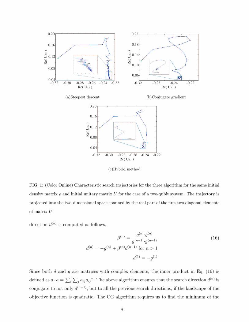
Re( U1,1 )

0.20

Re(

U2

,2 )

0.16

0.12

0.08

0.04-0.32 -0.30 -0.28 -0.26 -0.24 -0.22

(a)Steepest descent

Re( U1,1 )

0.22

Re(

U2,2 )

0.18

0.14

0.10

0.06

-0.32 -0.28 -0.24 -0.22

(b)Conjugate gradient

Re( U1,1 )

0.20

Re(

U2

,2 )

0.16

0.12

0.08

0.04

-0.32 -0.30 -0.28 -0.26 -0.24 -0.22

(c)Hybrid method

FIG. 1: (Color Online) Characteristic search trajectories for the three algorithm for the same initial

density matrix ρ and initial unitary matrix U for the case of a two-qubit system. The trajectory is

projected into the two-dimensional space spanned by the real part of the first two diagonal elements

of matrix U .

direction d(n) is computed as follows,

β(n) =g(n)·g(n)

g(n−1)·g(n−1)(16)

d(n) = −g(n) + β(n)d(n−1) for n > 1

d(1) = −g(1)

Since both d and g are matrices with complex elements, the inner product in Eq. (16) is

defined as a · a =∑

i

∑j aijaij

∗. The above algorithm ensures that the search direction d(n) is

conjugate to not only d(n−1), but to all the previous search directions, if the landscape of the

objective function is quadratic. The CG algorithm requires us to find the minimum of the

8

function along each search direction before beginning the next search direction. This is a one-

dimensional minimization problem for function f(λ) = E(ρ, Unew), where Unew = U ei λg(n).

We minimize f(λ) by evaluating it at three points, λ = 0 (at no additional cost), λ = 0.1

and λ = 0.2, and fit the function to a parabola. In the rare case of E(ρ, U (n)) > E(ρ, U (n−1))

(usually less than 5% of the time), the one-dimensional minimization obviously fails. In

this case, we simply replace this CG step by a steepest descent step and restart the CG

relaxation (resetting n = 1).

Fig 1(b) illustrates the trajectory of a typical CG minimization for the same density

matrix ρ and initial unitary matrix U as that in Fig. 1(a). As expected, the CG trajectory

does not show the zig-zag behavior as in the SD trajectory. As a result, the CG algorithm

usually takes less iterations than SD to converge. Unfortunately, the CG trajectory develops

chaotic spirals as the minimum is approached, slowing down the convergence. Since each

CG iteration requires more than one evaluation of the entanglement function, the overall

convergence speed for the CG algorithm is similar compared to that of SD (see Section II F).

E. Hybrid Method

Given the limitations of both SD and CG algorithms, we find that a much more efficient

algorithm can be constructed for entanglement minimization when we combine the two

together. In particular, it has been suggested that for highly non-quadratic landscape, a

good strategy is to reset the CG search direction to the steepest descent direction from time

to time. [13] Therefore, in the hybrid method, we separately perform both a steepest descent

step and a conjugate gradient step at each iteration. The actual step we take is the one

that gives us the lower entanglement value, i.e. by comparing E(ρ, UnewSD ) and E(ρ, Unew

CG ).

Even though one iteration in the hybrid method is more expensive than both SD and CG,

the algorithm is much more efficient because it takes much fewer iterations to converge. As

shown in Fig. 1(c), the trajectory from hybrid method does not display either zig-zag or

spiral characteristics. We suggest in passing that it would be worthwhile to test the hybrid

method to other optimization problems, such as protein folding or ab initio calculations,

whose objective function has a complex landscape.

9

F. Comparison of convergence speed

The entanglement of formation between two qubits (N = 4) has been derived analyti-

cally [6], which can be used as a benchmark for the numerical algorithms. We found that all

three gradient search algorithms reach the (global) minimum given by the analytic solution

with M = N = 4 starting from an aribitrary initial unitary matrix. This indicates that

there is only a single minimum for the entanglement as a function of U . While all three

methods converge to the correct results in this case, their computation time is different.

The algorithms are tested on 1, 000 randomly generated density matrices and initial

unitary matrices (the random measure µ is defined in Section IIIA). The search iterations

continues until the absolute error of the entanglement measured from the analytic result is

less than 10−12. The tests are performed using a Matlab program running on a Pentinum II

PC. The benchmark results are shown in Table I, which clearly demonstrates the superiority

of the hybrid method over the other two. The average computation time for the hybrid

method (HM) is 4 to 5 times shorter than that for SD and CG, while the number of iterations

is 6 to 8 times smaller. It is also worth noting that SD sometimes requires an exceptionally

large number of steps to converge. We therefore limit the total number of iterations for all

three algorithms to 10, 000, at which point the algorithm will abort and declare failure if

convergence is still not reached. 97 of the 1, 000 test cases failed when SD is used, while

none of the cases failed if either CG or HM is used. Thus the average time statistics for SD

would become even less favorable compared with the other two had we used an even larger

number for the maximum allowed steps. In the following, we will only use HM to collect the

statistics of entanglement. The HM program is re-implemented into C++, which is faster

than the Matlab version by 2 orders of magnitude.

G. Local and global minima

Because the definition of the entanglement of formation requires the solution of a global

minimization problem, it is of interest to find out whether the landscape of the entanglement

function have multiple local minima. In the case of two qubits (N = 4), we find that the

minimization algorithm (hybrid method) always converge to the analytic solution given

arbitrary initial unitary matrix U . This indicates that for N = 4 there is only a single

10

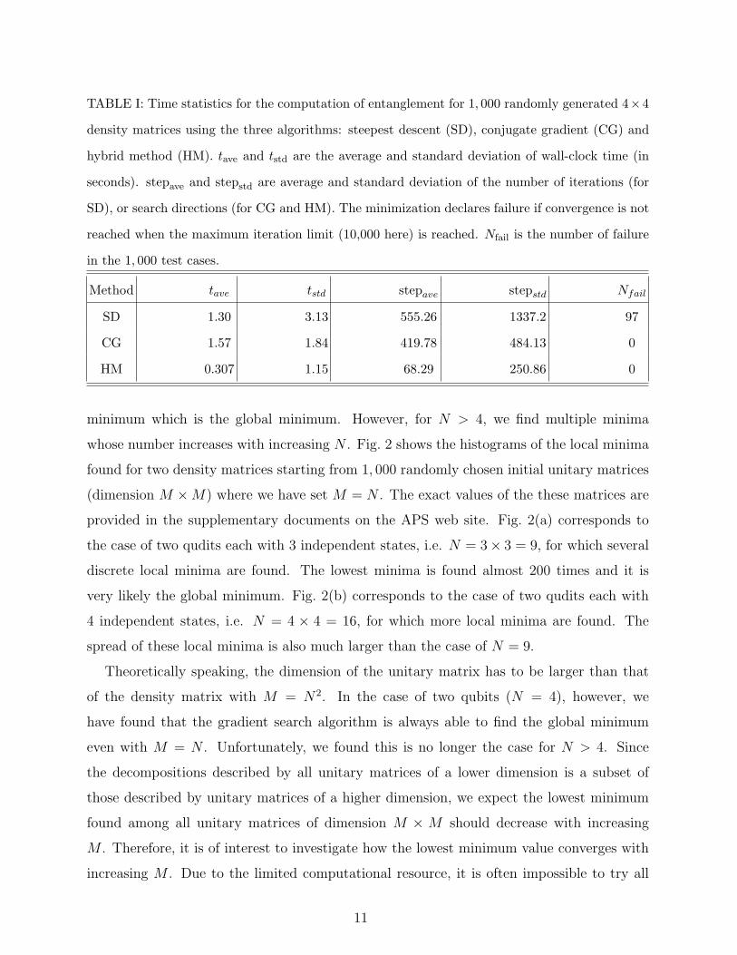
TABLE I: Time statistics for the computation of entanglement for 1, 000 randomly generated 4×4

density matrices using the three algorithms: steepest descent (SD), conjugate gradient (CG) and

hybrid method (HM). tave and tstd are the average and standard deviation of wall-clock time (in

seconds). stepave and stepstd are average and standard deviation of the number of iterations (for

SD), or search directions (for CG and HM). The minimization declares failure if convergence is not

reached when the maximum iteration limit (10,000 here) is reached. Nfail is the number of failure

in the 1, 000 test cases.

Method tave tstd stepave stepstd Nfail

SD 1.30 3.13 555.26 1337.2 97

CG 1.57 1.84 419.78 484.13 0

HM 0.307 1.15 68.29 250.86 0

minimum which is the global minimum. However, for N > 4, we find multiple minima

whose number increases with increasing N . Fig. 2 shows the histograms of the local minima

found for two density matrices starting from 1, 000 randomly chosen initial unitary matrices

(dimension M ×M) where we have set M = N . The exact values of the these matrices are

provided in the supplementary documents on the APS web site. Fig. 2(a) corresponds to

the case of two qudits each with 3 independent states, i.e. N = 3× 3 = 9, for which several

discrete local minima are found. The lowest minima is found almost 200 times and it is

very likely the global minimum. Fig. 2(b) corresponds to the case of two qudits each with

4 independent states, i.e. N = 4 × 4 = 16, for which more local minima are found. The

spread of these local minima is also much larger than the case of N = 9.

Theoretically speaking, the dimension of the unitary matrix has to be larger than that

of the density matrix with M = N2. In the case of two qubits (N = 4), however, we

have found that the gradient search algorithm is always able to find the global minimum

even with M = N . Unfortunately, we found this is no longer the case for N > 4. Since

the decompositions described by all unitary matrices of a lower dimension is a subset of

those described by unitary matrices of a higher dimension, we expect the lowest minimum

found among all unitary matrices of dimension M × M should decrease with increasing

M . Therefore, it is of interest to investigate how the lowest minimum value converges with

increasing M . Due to the limited computational resource, it is often impossible to try all

11

(a) (b)

0.076 0.078 0.08 0.0820

200

400

E

Freq

uenc

y

0.06 0.08 0.10

50

100

150

E

Freq

uenc

y

FIG. 2: (Color Online) Histogram of local minima of the entanglement function for two density

matrices of dimension N ×N , each obtained from gradient searches starting from 1, 000 different

initial decomposition matrices of dimension M × M with M = N . (a) N = 3 × 3 = 9. (b)

N = 4× 4 = 16. [17]

possible values of M from N to N2. For example, for two qudits each having 4 independent

states, N = 4× 4 = 16 and N2 = 256. If we let M = N2 then matrix U would have 65, 536

elements and matrix U would have 4096 elements. This is beyond the range of our current

computational power, especially because we still need to try many (e.g. 100) different initial

unitary matrices for each chosen M to ensure a fair chance of finding the global minimum.

We have tested the convergence of the lowest minimum as M increases from N to 2N .

When one of the two particles is a qubit (having only two independent states), changing M

from N to 2N does not change the lowest minimum value by more than 1%. In all other

cases, the lowest minimum seems to decay exponentially with increasing M and seem to

have converged well before M reaches 2N . This is a good sign because it suggests that

numerically it may not be necessary to ever go to the limit of M = N2. Fig. 3 illustrates

this convergence behavior for the case of N = 4 × 4 = 16. The lowest minimum value

obtained for different values of M is normalized by the value for M = N . The normalized

curve is then averaged over several hundred (200 for N > 10, 500 otherwise) random density

matrices, which leads to the curve in Fig. 3. The normalized and averaged entanglement

value is seen to converge exponentially,

E(M) = E0 + ∆E exp[−λ(M −N)] (17)

where the rate of convergence λ can be obtained empirically by numerical fitting. To see

whether the rate of convergence is large enough to justify stopping M at 2N , we can use

δE = ∆E exp(−λN) as an error estimator. The fitted values for λ and the error estimates

12

δE for various choices of N = nA×nB are shown in Table II, where nA and nB are the number

of independent states for particles A and B, respectively. In all the cases we have tested, this

error estimator never exceeds 10−3. Notice that the smallness of δE only indicates the self-

consistency for stopping M at 2N . It does not preclude the possibility that a substantially

lower minimum can be found for some M > 2N . As a compromise between numerical

accuracy and computational cost, we use M = 2N for all the calculations in Section III.

0 5 10 150

0.2

0.4

0.6

0.8

1

M−N

Ave

rage

Nor

mal

ized

Ent

angl

emen

t

FIG. 3: (Color Online) Minimum entanglement value obtained for different M normalized by the

value at M = N and then averaged over several hundred random density matrices for N = 4×4 =

16. The data is fitted to an exponential function E(M) = E0 + ∆E exp[−λ(M −N)] and the solid

line represents E0.

TABLE II: Fitted value of λ and ∆E in Eq. (17) and error estimate δE = ∆E exp(−λ N) for

various choices of N = nA × nB (see text).

N nA nB λ ∆E δE/E0

6 2 3 3.25 0.0005 1.2e-12

8 2 4 1.46 0.0025 2.2e-8

9 3 3 1.68 0.0273 7.0e-9

10 2 5 1.25 0.0046 1.6e-8

12 3 4 1.61 0.187 1.0e-8

15 3 5 0.71 0.257 1.8e-6

16 4 4 0.51 0.393 1.7e-4

13

III. ENTANGLEMENT STATISTICS IN RANDOM DENSITY MATRIX ENSEM-

BLE

In this section, we apply the gradient search algorithm developed in the previous section

to an ensemble of random density matrices and explore the correlation between entanglement

and other easier-to-compute quantities such as participation ratio and negativity.

A. Random density matrix ensemble

Before we can discuss the statistical distribution of the entanglement of randomly dis-

tributed density matrices, we first need to define a measure in the space of density matrices,

i.e. to specify the precise meaning of “randomly distributed”. Because there is no standard

definition for the measure in the space of density matrices, we follow the definition proposed

by Zyczkowski [7]. Recall that a density matrix is a positive semi-definite Hermitian matrix

with trace equal to one. A density matrix can always be diagonalized by a unitary trans-

formation, ρ = V DV †. Hence a measure µ of density matrix ρ can be constructed from the

measure ∆1 of the diagonal matrix D and the measure νH of the unitary matrix V , i.e.,

µ = ∆1 × νH . (18)

The measure ∆1 is a uniform distribution on the (N−1)-dimensional simplex determined by

the trace condition∑N

i Dii = 1. νH is the Haar measure for random unitary matrices. [9] To

generate a random density matrix, we first generate a random unitary matrix V according

to the Haar measure using the algorithm given in [9]. Another auxiliary random unitary

matrix U is generated by the same algorithm and the squared moduli of its first column is

used to generate the diagonal elements of matrix D,

Dii = |Ui1|2 (19)

The random density matrix is obtained by ρ = V DV †.

Using this procedure, we generate 10, 000 density matrices of dimension N ×N for every

N = 4, 6, 8, 9, 10, 12, 15, 16, as listed in Table III. Analytic solutions are used in the case of

N = 2 × 2. In higher dimensions, entanglement is obtained by the hybrid gradient search

algorithm with with M = 2N and the convergence criteria is set such that the average of

reduction of entanglement over the last 10 consecutive steps is less than 10−11. For each

14

density matrix, minimization is performed from 10 randomly chosen initial unitary matrices

and the lowest minimum value obtained among these 10 runs is used as the (upper-bound)

estimate of the global minimum. The entanglement results thus obtained are correlated with

other quantities that are believed to be related to entanglement, such as participation ratio

and negativity [7, 10, 15].

B. Participation ratio

The participation ratio R of a density matrix ρ is defined as,

R(ρ) =1

Tr(ρ2). (20)

Because R = 1 for certain pure states and R = N for totally mixed states (ρ = I/N), R

can be interpreted as an effective number of pure states in the mixture. Therefore we would

expect a decreasing entanglement E for an increasing R. Fig. 4 demonstrates the anti-

correlation between entanglement E and participation ratio R. As the participation ratio R

grows, especially when R exceeds a certain threshold value, the fraction of states with zero

entanglement (i.e. separable states) increases. In other words, purer quantum states (with

smaller R) tend to have a smaller probability to be decomposable into factorizable states.

C. Negativity and PPT states

The elements of a density matrix can be specified by ρjl,j′l′ where indices j and j′ cor-

responds to sub-system A and indices l and l′ corresponds to sub-system B. A partial

transpose of ρ is defined as(ρT2

)jl,j′l′ = ρjl′,j′l. (21)

in which only the indices for sub-system B are transposed. All of the eigenvalues of the

original density matrix ρ are non-negative. However, this is not the case for ρT2 . The

negativity parameter t is defined as a way to quantify the violation of this condition,

t ≡N∑i

|d′i| − 1, (22)

where d′i is the i-th eigenvalue of matrix ρT2 . Because the partial transpose does not alter

the trace,∑N

i d′i = 1 is still satisfied. Therefore, if any eigenvalue d′i is negative, t will

15

(a) (b)

(c) (d)

FIG. 4: (Color Online) Dots: correlation between entanglement E and participation ratio R for

10, 000 random N × N density matrices, where N = nA × nB. Solid line: fraction of zero entan-

glement states for a given participation ratio. (a) N = 2 × 2 (b) N = 2 × 3 (c) N = 3 × 3 (d)

N = 3× 5.

become positive. States with t = 0 are called positive partial transpose (PPT) states. It

has been shown that a separable state (i.e. E = 0) must have t = 0. [11] In other words,

a separable state must be a PPT state, but the converse is not true. It is also known that

all states with participation ratio R > N − 1 must have t = 0 and E = 0. [15] Given these

theoretical results, we expect a positive correlation between negativity t and entanglement

E, which is indeed supported by our numerical results, as shown in Fig. 5. For all the density

matrices that have R > N−1, we find that the entanglement reported by the gradient search

algorithm is always less than 10−9. This confirms the correctness of the theoretical result as

well as the robustness of our numerical algorithm. [15]

Some statistics of our numerical results are summarized in Table III. The correlation

function S(E, t) is found to be close to 1 for all the cases, supporting a strong correlation

between entanglement and negativity. While it has been shown that for N = 4 and N = 6,

a density matrix is separable (E = 0) if and only if it is a PPT state (t = 0), for N > 6 there

exist PPT states with non-zero entanglement. For N = 8, Zyczkowski [7] estimated the

16

(a) (b)

0 0.5 10

0.5

1

tE

0 0.5 10

0.5

1

t

E

(c) (d)

0 0.5 10

0.5

1

t

E

0 0.5 10

0.5

1

tE

FIG. 5: (Color Online) Correlation between entanglement E and negativity t for 10, 000 random

N × N density matrices, where N = nA × nB. (a) N = 2 × 2 (b) N = 2 × 3 (c) N = 3 × 3 (d)

N = 3× 5.

fraction of separable states among PPT states to be only 78.7% [7]. Our numerical results

can also be used to estimate the fraction of separable states among PPT states.

Due to limited numerical resolution, we classify all density matrices with E < 10−9 as

separable states, i.e. E = 0. Consistent with the previous report [10], all PPT states

are separable for N ≤ 6. Strikingly, we also found that all PPT states among the 10, 000

randomly generated density matrices (including N = 8) have zero entanglement regardless

of dimension. This contradicts previous report [7] and suggests that the fraction of separable

states among PPT states is close to 100% for the case of N = 2 × 4. The disagreement

is mostly due to the faster convergence of our gradient search algorithm, which allows us

to use many initial unitary matrices to obtain a better estimate of the global minimum.

Nonetheless, our results should not be over-interpreted as: all PPT states are separable

states. In fact, Horodecki [14] has provided an example of non-separable PPT states for

17

TABLE III: Statistics of 1, 000 random density matrices of different dimensions. Eave and tave is

the average entanglement and negativity. S(E, t) = Cov(E, t)/[Var(E)Var(t)]1/2 is the correlation

between E and t. PPPT is the fraction of PPT states among all the sampled random density

matrices.

N nA nB Eave tave S(E, t) PPPT

4 2 2 0.0308 0.0568 0.9699 0.630

6 2 3 0.0423 0.0763 0.9732 0.390

8 2 4 0.0482 0.0857 0.9767 0.236

9 3 3 0.0578 0.0969 0.9765 0.165

10 2 5 0.0499 0.0891 0.9799 0.141

12 2 6 0.0531 0.0941 0.9821 0.078

12 3 4 0.0655 0.1070 0.9787 0.071

15 3 5 0.0707 0.1144 0.9798 0.029

16 4 4 0.1573 0.1314 0.9685 0.002

N = 2× 4,

ρb =1

7b + 1

b 0 0 0 0 b 0 0

0 b 0 0 0 0 b 0

0 0 b 0 0 0 0 b

0 0 0 b 0 0 0 0

0 0 0 0 α 0 0 β

b 0 0 0 0 b 0 0

0 b 0 0 0 0 b 0

0 0 b 0 β 0 0 α

(23)

where α = 12(1+b) and β = 1

2

√1− b2. For arbitrary b ∈ (0, 1), this state has negativity t = 0,

but non-zero entanglement E and participation ratio R. Here we compute the entanglement

E as a function of b using the HM algorithm with M = 2N . Fig. 6 plots the entanglement

E and participation ratio R as functions of b. It is likely that states in this family of density

matrices occupies a negligible volume in the ensemble of random density matrices, which is

why we did not observe any non-separable PPT states in all of our 10, 000 density matrices

(23.6% are PPT states).

18

(a) (b)

0 0.5 10

0.01

0.02

bE

0 0.5 11

2

3

4

5

b

R

FIG. 6: (Color Online) (a) Entanglement E of the Horodecki state, Eq. (23), as a function of b.

(b) Participation ratio R as a function of b.

To test this hypothesis, we generate several ensembles of density matrix by randomly

perturbing the Horodecki matrix, Eq. (23), with b = 0.2 where the entanglement is close to

the local maximum. First, we found that by replacing all zero components in Eq. (23) by

a small positive number γ, the resulting density matrix is still a bound entangled state, as

long as 0 < γ < 0.01 b. However, the density matrix is no longer PPT if γ is too large or

if the zero components in Eq. (23) are perturbed randomly (i.e. not replaced by the same

value γ).

Second, we decompose the Horodecki state into a weighted sum of 16 pure states as in

Eq. (7) by using random 16 × 16 unitary matrices. We then perturb all pure states wi by

adding a random number ξ that is uniformly distributed in the domain [−∆, ∆] to every

component. Each perturbed state is then normalized and the normalization constant is

multiplied to the assigned probability of this state. The total probability of all states is then

renormalized to unity. A new density matrix is obtained by summing up the contributions

from each pure state. We have studied four different cases with ∆ = 0.01b, 0.1b, b, 10b,

respectively. 10, 000 random matrices are generated in each case, and the number of PPT

states observed are 2, 24, 2816, 4712, respectively. For ∆ = 0.01b and 0.1b, all the PPT

states are bound entangled states. However, for ∆ = b and 10b, none of the PPT states

generated are entangled.

We would like to make the following conjectures based on the above results. First, a

small volume of bound entangled states exists at the vicinity of Horodecki matrix, and

they are very difficult to find. For example, in the second approach described above, we

only found 26 of such states out of 40, 000 random matrices. Second, large perturbations

19

to the Horodecki matrix lead to an ensemble of density matrices with similar statistical

behavior as the ensemble generated earlier in Section.III.A, i.e., all these PPT states have

zero entanglement. Given that we are able to generate a few bound entangled states by

randomly perturbing the Horodecki matrix (with ∆ ≤ 0.1b), the fraction of bound entangled

states among PPT states can be a finite but very small number.

IV. SUMMARY

We develop a fast gradient search algorithm for the computation of the entanglement of

formation for a mixed state, which is defined as the smallest average entanglement among

all possible ways to decompose the mixed state into a classical mixture of pure states.

This is enabled by the analytic derivatives of entanglement with respect to the unitary

decomposition matrix, which are given in Appendix A. A hybrid method, combining steepest

descent and conjugate gradient methods, is found to outperform both of them. The fast

convergence of the hybrid method allows us to compute entanglement of formation in higher

dimensions than what was possible before. Nonetheless, the hybrid method still searches for

the local minimum only. In order to estimate the global minimum, we repeat the gradient

search several times starting from different random initial conditions and select the lowest

local minimum obtained from all the searches. In principle, the gradient search algorithm

presented here can be combined with other techniques, such as the simulated annealing [16]

or genetic algorithm [8] to expedite the search for the global minimum.

Using the hybrid gradient search algorithm, we obtained entanglement statistics of 10, 000

density matrices with N ranging from 2× 3 to 4× 4. Anti-correlation is observed between

entanglement E and participation ratio R, whereas a strong correlation is observed between

E and negativity t. In particular, all the PPT states (density matrices with t = 0) in our

study are found to be separable (E = 0). This suggests a much higher ratio of separable

states among PPT states than reported earlier, most likely due to the better convergence of

our numerical results.

20

APPENDIX A: DERIVATIVES OF E WITH RESPECT TO U

Consider the entanglement E as a function of both the density matrix ρ and the decom-

position matrix U ,

E(ρ, U) =M∑i=1

pi E(ρAB(i)) (A1)

where ρAB(i) = |wi〉〈wi| is the density matrix of the pure state |wi〉. The entanglement of a

pure state is defined through the von Neuman entropy of the partial trace,

E(ρAB(i)) ≡ S(ρA(i)) = −Tr[ρA(i) log2 ρA(i)

](A2)

ρA(i) = TrB

[ρAB(i)

](A3)

In this appendix, we derive the derivative of E with respect to every component of U . It

is important to note that the components Uij are complex numbers. We will treat Uij and

U∗ij (the complex conjugate) as independent variables. In other words, the change δE with

caused by a small change of matrix U can be written as,

dE =∑ij

∂E

∂Uij

dUij +∂E

∂U∗ij

dU∗ij (A4)

Computing the derivative of E with respect to U requires the derivatives of both pi and

S(ρ(i)A ) with respect to U , i.e.,

∂E(ρ)

∂Ukl

=M∑

h=1

[∂ph

∂Ukl

S(ρA(h)) + ph∂S(ρA(h))

∂Ukl

]. (A5)

The derivative of pi is easier to obtain,

∂ph

∂Ukl

= λlU∗hlδkh , (A6)

where λl is the eigenvalue of ρ.

To obtain the derivative of S(ρ(i)A ), we need to follow the chain rule,

S(ρA(i)) → ΛA(i)p → ρA(i) → ρAB(i) → |wi〉 → U. (A7)

where ΛA(i)p is the p-th eigenvalue of matrix ρA(i), based on which S(ρA(i)) can be written as,

S(ρA(i)) = −nA∑p=1

ΛA(i)p log2(Λ

A(i)p ) (A8)

21

Therefore,

∂S(ρ(h)A )

∂ΛA(h)p

= − log2(eΛA(h)p ) (A9)

Continue with the chain rule,

∂ΛA(h)p

∂Ukl

=N∑

r,s=1

nA∑t,u=1

∂ΛA(h)p

∂ρA(h)tu

∂ρA(h)tu

∂ρAB(h)rs

∂ρAB(h)rs

∂Ukl

. (A10)

Let A(h) be the matrix that diagonalize the density matrix ρA(i),

ρA(i) = A(h)DA(h)A(h)† (A11)

where DA(h)pp = Λ

A(h)p . We can show that

∂ΛA(h)p

∂ρA(h)tu

= A(h)∗tp A(h)

up (A12)

The middle term in the r.h.s. of Eq. (A10) is either zero or one, depending on the indices t,

u, r and s,

∂ρA(h)tu

∂ρAB(h)rs

=

nB−1∑n=0

δ(t+n·nA),rδ(u+n·nA),s, (A13)

To find the last term in the r.h.s. of Eq. (A10), we first find that,

∂(phρAB(h)rs )

∂Ukl

= δkh Wrh V ∗sl (A14)

Finally,

ph∂ρ

AB(h)rs

∂Ukl

=∂(phρ

AB(h)rs )

∂Ukl

− ρAB(h)rs

∂ph

∂Ukl

(A15)

= δkh

(WrhV

∗sl − ρAB(h)

rs λlU∗hl

)(A16)

Combining all results together, we have

∂E(ρ, U)

∂Ukl

= λl U∗kl S(ρA(k))−

nA∑p=1

log2(eΛA(k)p )

×N∑

r,s=1

nA∑t,u=1

A(h)tp

∗A(h)

up

(WrkV

∗sl − ρAB(k)

rs λlU∗kl

)(

nB−1∑n=0

δt+nnA,r δu+nnA,s

)(A17)

22

APPENDIX B: STEEPEST DESCENT DIRECTION FOR HERMITIAN MA-

TRIX H

In this appendix, we show that the steepest descent direction for Hermitian matrix H

(defined by U = eiH) is

g =1

2

[(iU †G∗

)+

(iU †G∗

)†](B1)

First, recall that we treat Uij and its complex conjugate U∗ij as independent variables. This

means that a differential change of E can be written as

dE =M∑i=1

N∑j=1

GijdUij + G∗ijdU∗

ij (B2)

where

Gij =∂E(ρ, U)

∂Uij

(B3)

is the derivative we obtained in Appendix A. It can be verified that, if matrix U were not

subject to any constraints, the steepest descent direction for Uij should be −G∗ij, instead of

−Gij itself.

To impose the unitary constraint, we let

Unew = U eiδH (B4)

where δH is a small Hermitian matrix. Hence the change of matrix U is,

δU = Unew − U = i U δH (B5)

to the first order of δH. For convenience, we define a square matrix G whose first N columns

are identical to G, while other columns are filled with zeros. The ensuing change of E is,

dE =M∑

i=1,k=1

N∑j=1

i GijUikδHkj − i G∗ijU

∗ikδH

∗kj

=M∑

i=1,j=1,k=1

i GijUikδHkj − i G∗ijU

∗ikδH

∗kj

=M∑

k=1

M∑j=1

(i UT G)kj δHkj + (i UT G)∗kj δH∗kj

23

Since δH is a Hermitian matrix, δHkj = δH∗jk. Hence,

dE =M∑

k=1

M∑j=1

(i UT G)kj δHkj + (i UT G)∗kj δHjk

=M∑

k=1

M∑j=1

[(i UT G)kj + (i UT G)∗jk

]δHkj

=M∑

k=1

M∑j=1

[(i UT G) + (i UT G)†

]kj

δHkj

=M∑

k=1

M∑j=1

1

2

[(i UT G) + (i UT G)†

]kj

δHkj

+1

2

[(i UT G) + (i UT G)†

]∗kj

δH∗kj (B6)

Hence the steepest descent direction for H is,

g = −1

2

[(i UT G) + (i UT G)†

]∗

=1

2

[(i U † G∗) + (i U † G∗)†

](B7)

ACKNOWLEDGMENTS

We wish to thank Prof. Sandu Popescu and Dr. Patrice E. A. Turchi for first introducing

us to the problem of entanglement computation. This work was performed under the aus-

pices of the US Department of Energy by the University of California, Lawrence Livermore

National Laboratory under Contract No. W-7405-Eng-48. Seunghwa Ryu acknowledges

support from a Weiland Family Stanford Graduate Fellowship.

[1] M. A. Nielson and I. I. Chuang, Quantum Computation and Quantum Information, Cambridge

University Press (2000).

[2] P. W. Shor, Algorithms for Quantum Computation: Discrete Logarithm and Factoring (1994).

[3] E. Schrodinger, Proc. Cambridge. Philos. Soc. 31, 555 (1935).

[4] J. S. Bell, Physics 1, 195 (1964).

[5] C. H. Bennett, D. P. DiVincenzo, J. A. Smolin, and W. K. Wootters, Phys. Rev. A 54, 3824

(1996).

24

[6] W. K. Wootters, Phys. Rev. Lett. 80, 2245 (1998).

[7] K. Zyczkowski, Phys. Rev. A 60, 3496 (1999).

[8] R. V. Ramos, J. Comput. Phys. 192, 95 (2003).

[9] M. Pozniak, K. Zyczkowski, and M. Kus, J. Phys. A31, 1059 (1998).

[10] K. Zyczkowski, P. Horodecki, A. Sanpera, and M. Lewenstein, Phys. Rev. A 58, 883 (1998).

[11] A. Peres, Phys. Rev. Lett. 77, 1413 (1996).

[12] Payne et al., Rev. Mod. Phys. 64, 1045 (1992).

[13] E. K. P. Chong and S. H. Zak, An Introduction to Optimization, John Wiley & Sons, INC.

(1996).

[14] P. Horodecki, Phys. Lett. A 232, 333 (1997)

[15] L. Gurvits and H. Barnum, Phys. Rev. A 66, 062311 (2002).

[16] S. Kirkpatrick, C. D. Gelatt, and Jr., M.P. Vecchi, Science 220, 4598, 671 (1983).

[17] See EPAPS Document No. [ ] for density matrices examined to obtain the histograms.

[18] ei(H+δH) = eiH · eiδH only in the limit of infinitesimal δH. But Eq. (13) remains a unitary

matrix for arbitrary Hermitian matrix δH.

25