Quantum Computation‘ NORMAN MARGOLUS

Laboratory for Computer Science Massachusetts Institute of Technology

Cambridge, Massachusetts 021 39

INTRODUCTION

When we describe the operation of a computer, we are of course describing the dynamical evolution of physical system. What distinguishes a computer from other physical systems is its ability to simulate many aspects of other physical processes (including, in particular, the logical operation of any other computer, given enough time and memory’). It is interesting to note that for several recent models of computation, the mapping between the computer and the underlying physics is quite direct. This leads us to ask the question: “how similar can the models used to describe computers be made to microscopic physics?”

This question is of some interest to the technologists because it is closely related to how efficiently and quickly physical degrees of freedom can be made to perform a computation for us.’ Models in which there is a very direct mapping between the computational and the physical degrees of freedom can also act as bridges connecting concepts and techniques in physics and computation.’

A particularly simple classical-mechanical model of computation was found by Fredkin: He showed that a gas of hard spheres with exactly prescribed initial conditions can be made to perform an arbitrary digital computation. This and other related logically reversible models of computationb have played a critical theoretical role in establishing the possibility of microscopic physical models of computation. They have also helped in clarifying issues related to fundamental thermodynamic constraints on the computational proce~s.’~ But of course the world is quantum mechanical, and so what we would really like is a quantum model of computation.

It may well be that to take best advantage of the computational capabilities of Q M systems, we must reformulate our notion of a computation. However, in this paper, I will restrict my attention to the more straightforward problem of asking to what extent

‘This research was supported by grants from the Defense Advanced Research Projects Agency (N00014-83-K-0125), the National Science Foundation (82143 12-IST). and the Department of Energy (DE-AC02-83ER13082).

’Computers that operate invertibly at every step have been de~cribed~*~*~.’ and are found to be essentially not much more complex or difficult to use than conventional computers. It was a significant and somewhat surprising discovery that general-purpose computation can be carried out in a reasonable manner despite the severe constraints implied by invertible operation. In a reversible computer, no information can be lost at any step of the computation-you cannot simply erase unneeded partial results, or even the arguments to an addition. One way of effectively “erasing” partial results is to copy an answer once you have it, and then do an inverse computation so that all intermediate results go away and only the initial inputs and a copy of the answer remain.

487

488 ANNALS NEW YORK ACADEMY OF SCIENCES

a microscopic QM system can simulate an ordinary (classical) deterministic computa- tion.‘ I will describe some of the work that has been done in this direction and point out some difficulties that remain. As a specific model for illustration, I will use a reversible cellular automaton model of computation that is closely related to the hard-sphere-gas computer mentioned above, and address the issues of spatial locality, cyclic operation, and parallelism in quantum computation.

APPROACHES TO QUANTUM COMPUTATION

I will discuss two approaches to the issue of Quantum Computation (QC). Because the time-evolution operator in QM is always a unitary (and hence invertible) operator, both approaches will be based on the notion of a reversible computer. The two approaches will be distinguished by whether the time-evolution operator or the Hamiltonian operator is taken as the starting point for the discussion.

Time-Evolution Operator Approach

The first discussion indicating that QC was not necessarily inconsistent with the formalism of QM was that of Paul Benioff.’* It depends upon the observation that the Schrtidinger evolution of the wave function is perfectly deterministic. If one associates a basis vector with each possible logical state of a reversible computer, then the one-step time-evolution that carries each state into the appropriate next state is a permutation on the set of basis states; therefore, it is given by a unitary operator. Formally, it is always possible to write down an Hermitian operator whose complex exponential equals this unitary operator. Given an initial logical-basis state, the Schrodinger evolution generated by this Hamiltonian will give the appropriate successor logical states at consecutive integer timesd

For example, if we let the possible configurations of the three-state “computer” described in FIGURE 1 be represented by

‘We will not consider here the very interesting issue of a computer that is a Universal Quantum Simulator.” Such a computer would be a QM system that, started from an appropriate initial state corresponding to a state of any given QM system, would evolve in time, t , proportional to that taken by the given system into a QM state corresponding to the t-evolved state of the given system. Measurements performed on the simulator would correctly reproduce the QM statistics that one would have obtained by performing an experiment on the original system. Such a simulator would provide an alternative to the present computational methods used to predict the consequences of QM models. Deutsch” discusses this problem, but does not address the important issue of the spatial locality of the Hamiltonian.

dAlthough the SchrMinger equation is a linear differential equation, in QM we allow a large enough set of basis vectors (one per configuration) so that a unitary operator can take a computer through an arbitrary invertible sequence of configurations. In particular, there is no difficulty in having the computer compute such “nonlinear” functions as logical AND and OR.

MARGOLUS: QUANTUM COMPUTATION 489

then the time-evolution given in FIGURE 1 can be represented by the unitary single-time-step operator,

Then from U, we can find an Hermitian matrix such that U = e-jH. In this case,

H =

A 7 r 0 - _ -

2 2

7 r P -- - 0 2 2

0 0 0

FIGURE 1. A simple three-state machine. If the "computer" is in state A, it will go into state B. State B goes into A, and C does not change.

Hamiltonian Operator Approach

One would like the Hamiltonian operator, H, to be given as a sum of pieces, each of which only involves the interaction of a few parts of the computer that are near to each other. The most direct way of ensuring that H is of this form is to write H down ab initio, rather than derive it from U.

Richard Feynman was the first to discuss this appr~ach. '~ He realized that if the unitary operator, F, that describes one step of the desired forward evolution can be written as a sum of local pieces, then if we let H = F + Ft be the Hamiltonian operator, H will also be a sum of local (i.e., nearby-neighbor) interactions. The time-evolution operator, U(t) = e-i"f, is then a sum of powers of F and F' taken with various weights. Thus, if In) corresponds to the logical state of a computer at step n (i.e., Fln) =

In + l ) ) , then U(t) ln) is a superposition of configurations of the computer at various steps in the original computation. This superposition contains no configurations that are not legitimate logical successors or predecessors to In): if you make a measurement of the configuration of the computer, you will find it at some step of the desired

490 ANNALS NEW YORK ACADEMY OF SCIENCES

computation. If, instead, you simply measure some piece of the configuration that tells you whether the computation is done or not, then when you see that it is done, you can immediately look elsewhere in the configuration to find the answer and be assured that it is correct. Alternatively, one may construct a superposition of configuration states that acts as a sort of wave-packet state in which the computation moves forward at a uniform rate.

In order to write F = ZFi with F as a unitary operator, Feynman described a computer in which only one spot is active at a time. If instead of taking ZFi to be unitary we only require the F,'s to be local, it turns out that we can describe a computer where all sites are active at once, but where there is no longer a global time; that is, synchronization becomes a matter of local intercommunication.

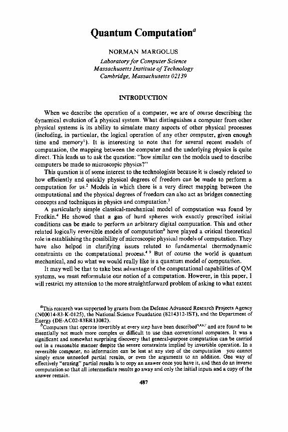
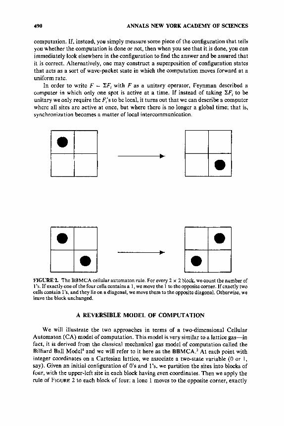
FIGURE 2. The BBMCA cellular automaton rule. For every 2 x 2 block, we count the number of 1 's. If exactly one of the four cells contains a 1, we move the 1 to the opposite corner. If exactly two cells contain l's, and they lie on a diagonal, we move them to the opposite diagonal. Otherwise, we leave the block unchanged.

A REVERSIBLE MODEL OF COMPUTATION

We will illustrate the two approaches in terms of a two-dimensional Cellular Automaton (CA) model of computation. This model is very similar to a lattice gas-in fact, it is derived from the classical mechanical gas model of computation called the Billiard Ball Model4 and we will refer to it here as the BBMCA.' At each point with integer coordinates on a Cartesian lattice, we associate a two-state variable (0 or 1, say). Given an initial configuration of 0's and l's, we partition the sites into blocks of four, with the upper-left site in each block having even coordinates. Then we apply the rule of FIGURE 2 to each block of four: a lone 1 moves to the opposite corner, exactly

MARGOLUS QUANTUM COMPUTATION 49 1

two 1’s on a diagonal switch to the other diagonal, and all other cases remain unchanged. Now we change the grouping of sites so that the upper-left site in each block of four has odd coordinates, and we again apply the BBMCA rule to all blocks. We iterate this procedure to generate a dynamical evolution.

The evolution generated by this rule is exactly invertible: this property is inherited from the invertibility of the rule applied to each block. Furthermore, it has been shown3 that starting from a suitable initial state, this system can do any computation that any general-purpose digital computer can do (1’s move around on the lattice, act as signals, and interact with each other to do digital logic, much like the logic that goes on in the circuitry of any electronic digital computer).

This model is an obvious candidate for us to try to describe in terms of a lattice of QM spins. Here QM may even be superior to classical mechanics because it is more natural to have identical two-state systems in QM (cf. references 2 and 9). During one logical step in such a CA model, information has only to be communicated to nearby neighboring spins; data-paths are very short and so the impact of the finite light-speed restriction on computation speed is minimized.‘

TIME-EVOLUTION OPERATOR APPROACH

In order to implement the BBMCA rule as a QM model, we will consider a two-dimensional lattice of spins, each of which is in a spin-component eigenstate with respect to the z-direction (which is taken to be perpendicular to the plane of the lattice). At each site, spin-up represents a logical 1 and spin-down represents a logical 0.

At a given lattice site with coordinates ( i , j ) , the projection operator, 5 =

(1 + ~ : ~ ) / 2 , projects states that have a logical 1 at site (i, j ) , and the operator, Pij =

(1 - ufj)/2 = 1 - Pij, projects states with 0 at (i, j ) . The operator, qj = (u; - i0;) /2 ,

lowers a I at (i, j ) to a 0, while ui = (a; + iu$)/2 raises a 0 at (i, j ) to a 1. We can now construct a unitary operator that will implement the BBMCA rule

applied to a block of four sites, with the upper-left corner at position (i, j ) : - -

Aij = (aijd+lj+l + a:ai+lj+l)Pi+ljQ+l

+ (ai+ ljai+ I + 4t ljaij+ 1) PijPi+ l j + I

+ (aija!+J G+ lai+ l j + I-+ a:ai+ ljaij+L4? l j + I I _

+ 1 - (EjPi+lj+l + Pi+lj&jtl - 2 ~ i j ~ i + ~ j ~ i j + ~ ~ , t ~ j + ~ ) .

-

If A,, is applied to a configuration of 1’s and O’s, all of the lattice sites, except those in the block at (i, j ) , will remain unchanged; this block will change according to the BBMCA rule. If we let

eOnly for computations that can take advantage of this architecture. For example, many problems that are usually described in terms of differential equations seem well suited to a CA so l~ t ion . ’~ . ’~

492 ANNALS NEW YORK ACADEMY OF SCIENCES

then U = UIUo is a unitary operator that exactly implements the BBMCA rule! U(t) =

U*/* will exactly correspond to a BBMCA evolution at even-integral times. Now we will try to write U(t) = e-iHf, with H a s a sum of local pieces. We begin by

noting that A; = 1 (which follows from the BBMCA rule). Therefore, [(l - A,)/2]' =

(1 - Aij)/2 and exp [ -iT( 1 - 4 / 2 1 = A, (expand the exponential). If we let Hij =

T (1 - Aij)/2, then

Uo = n A, = &%-HII, U - e - G , ~ H ~ 1 - ,,wen

and U(t) = e-IHt, where H= Zi,e,,Hi, when the integer part o f t is even and H = X,,ddH,J when it is odd.

This U will reproduce the BBMCA evolution- at all integer times. Intuitively, the reason we had to introduce a time dependence into H i s because the Hli s at a single

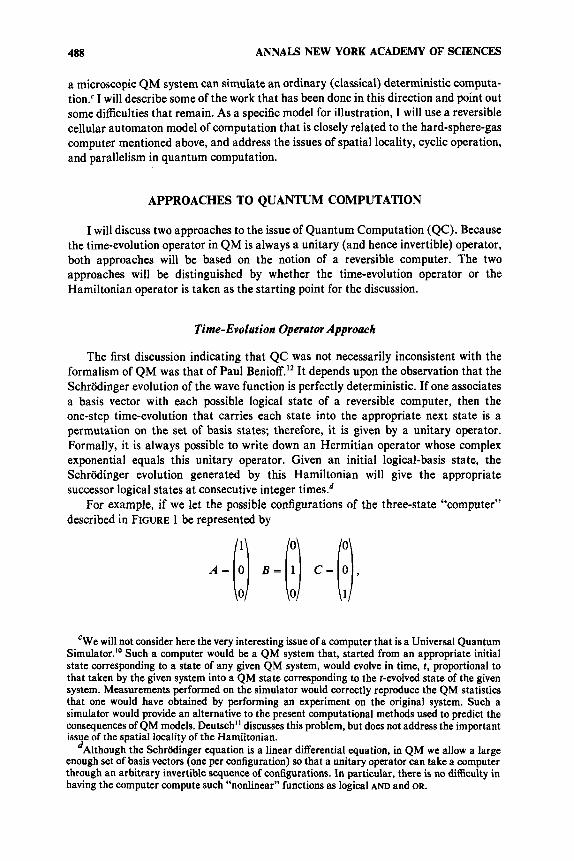
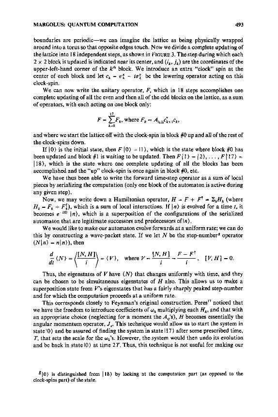
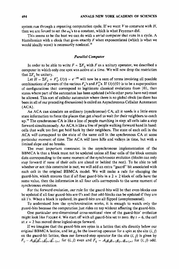
F i r s t 9 steps. N e x t 9 steps. FIGURE 3. A 6 x 6 lattice with periodic boundaries. All 2 x 2 blocks in the solid partition are updated first and then all blocks in the dotted partition are updated. Because of periodicity, numbers 9 through 17 mark the centers of dotted blocks.

time-step all refer to nonoverlapping blocks of spins, and so they all commute, thus allowing the product U, or (Il of exponentials to be turned into an exponential of a sum. The even-block and odd-block Hij's do not all commute-because the blocks overlap, it makes a difference in which order the Hiis are applied.

HAMILTONIAN OPERATOR APPROACH

Serial Computer

We can use Feynman's method to arrive at a time-independent version of the BBMCA. We will use a 6 x 6 lattice (FIGURE 3) to illustrate the technique. The

'It has been s~gges t ed '~* '~ that in order to construct a time-independent Nfor a Usuch as this, it is necessary to know explicitly the configuration of 1's and 0 s at each step of every possible computation in advance.

MARGOLUS QUANTUM COMPUTATION 493

boundaries are periodic-we can imagine the lattice as being physically wrapped around into a torus so that opposite edges touch. Now we divide a complete updating of the lattice into 18 independent steps, as shown in FIGURE 3. The step during which each 2 x 2 block is updated is indicated near its center, and ( ik , j , ) are the coordinates of the upper-left-hand corner of the Ph block. We introduce an extra "clock" spin at the center of each block and let c, = a; - iu; be the lowering operator acting on this clock-spin.

We can now write the unitary operator, F, which in 18 steps accomplishes one complete updating of all the even and then all of the odd blocks on the lattice, as a sum of operators, with each acting on one block only:

17 F = Z F k , where F k = A i , j k C i , l C k ,

k-0

and where we start the lattice off with the clock-spin in block #O up and all of the rest of the clock-spins down.

If (0) is the initial state, then F ( 0 ) = Il), which is the state where block #O has been updated and block #I is waiting to be updated. Then F 11 ) = 12), . . . , F 117) =

)18), which is the state where one complete updating of all the blocks has been accomplished and the "up" clock-spin is once again in block #0, etc.

We have thus been able to write the forward time-step operator as a sum of local pieces by serializing the computation (only one block of the automaton is active during any given step). - &Hk (where Hk = Fk + F f ) , which is a sum of local interactions. If In) is evolved for a time t, it becomes eci''' In), which is a superposition of the configurations of the serialized automaton that are legitimate successors and predecessors of In).

We would like to make our automaton evolve forwards at a uniform rate; we can do this by constructing a wave-packet state. If we let N be the step-numberg operator (NI n) = n I n)), then

Now, we may write down a Hamiltonian operator, H = F +

" , H I F - F' = ( V ) , where V = - = - 9 EV,:Hl -0.

2 i

Thus, the eigenstates of V have ( N ) that changes uniformly with time, and they can be chosen to be simultaneous eigenstates of H also. This allows us to make a superposition state from V's eigenstates that has a fairly sharply peaked step-number and for which the computation proceeds at a uniform rate.

This corresponds closely to Feynman's original construction. Peres" noticed that we have the freedom to introduce coefficients of wk multiplying each H,, and that with an appropriate choice (neglecting for a moment the Ai,'s), H becomes essentially the angular momentum operator, J,. This technique would allow us to start the system in state 10) and be assured of finding the system in state 117) after some prescribed time, T, that sets the scale for the w i s . However, the system would then undo its evolution and be back in state 10) at time 2T. Thus, this technique is not useful for making our

glO) is distinguished from 118) by looking at the computation part (as opposed to the clock-spins part) of the state.

494 ANNALS NEW YORK ACADEMY OF SCIENCES

system run through a repeating computation cycle. If we want Y to commute with H , then we are forced to set the up’s to a constant, which is what Feynman did.

This seems to be the best we can do with a serial computer that runs in a cycle. A Hamiltonian with a clock that gives exactly F when exponentiated (which is what we would ideally want) is necessarily nonlocal.IE

Parallel Computer

In order to be able to write F = ZFij with F as a unitary operator, we described a computer in which only one spot was active at a time. We will now drop the restriction that ZFi, be unitary.

Let H = ZFjj + Fb. V ( f ) = e-j”’ will now be a sum of terms involving all possible combinations of powers of the various Fiis and F t s . If U(t) (0) is to be a superposition of configurations that correspond to legitimate classical evolutions from I O), then states where part of the automaton has been updated (while other parts have not) must be allowed, This sort of cellular automaton where there is no global clock (as there has been in all of our preceding discussions) is called an Asynchronous Cellular Automaton (ACA).

An ACA can simulate an ordinary (synchronous) CA; all it needs is a little extra state information to force the places that get ahead to wait for their neighbors to catch up.19 The synchronous CA is like a line of people marching in step: all cells take a step forward simultaneously. An ACA is like a line of people walking forward hand in hand: cells that walk too fast get held back by their neighbors. The state of each cell in the ACA will correspond to the state of the same cell in the synchronous CA at some particular moment of time. The ACA will have hills and valleys in time, but with a limited slope and no breaks.

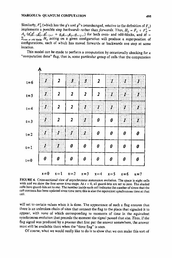
The most important constraint in the asynchronous implementation of the BBMCA is that a block must not be updated unless all four cells of the block contain data corresponding to the same moment of the synchronous evolution (blocks can only step forward if none of their cells are ahead or behind the rest). To be able to tell whether or not this constraint is met, we will add an extra “guard” bit associated with each cell in the original BBMCA model. We will make a rule for changing the guard-bits, which ensures that if all four guard-bits in a 2 x 2 block of cells have the same value, then the information in all four cells corresponds to the same moment of synchronous evolution.

For the forward evolution, our rule for the guard-bits will be that even-blocks can be updated if all four guard-bits are 0’s and that odd-blocks can be updated if they are all 1’s. When a block is updated, its guard-bits are all flipped (complemented).

To understand how the synchronization works, it is enough to watch only the guard-bits because the computation just rides on top without affecting the guard-bits.

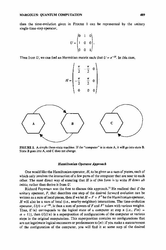
One particular one-dimensional cross-sectional view of the guard-bits’ evolution might look like FIGURE 4. We start off with all guard-bits set to zero. By t = 6, the cell at x = 2 has moved three logical-steps forward.

If we imagine that the guard-bits are spins in a lattice that sits directly below our original BBMCA lattice, and let gij be the lowering operator for a spin at the site ( i , j ) on the guard-bit lattice, then our forward-step operator for the site (i, j ) is given by Fij = Ajjg~g~+l,g~+,g~+y+, for (i, j ) even and Fu = Aijgijgj+ljgij+Igi+lj+, for (i, j ) odd.

MARCOLUS QUANTUM COMPUTATION 495

: : : J : : :

:: .$::

0

. . . . .............. ..............

Similarly, Fi. (which has the g’s and gt’s interchanged, relative to the definition of F,) implements a possible step backwards rather than forwards. Thus, Hi, = Fij + FL =

A, (g~g~+,jg~+,g~+lj+I + gijgi+,jgij+lgi+,j+I) for both even- and odd-blocks, and H =

Z,,, o, ,,,,,, blocks Hij acting on a given configuration will produce a superposition of configurations, each of which has moved forwards or backwards one step at some location.

This model can be made to perform a computation by occasionally checking for a “computation done” flag; that is, some particular group of cells that the computation

............................ ............................

. . . . . . . . . . . . . . . . . . . . 0 0 0 0 113::: ::y::: ::g:::

0 0 0 0 0 0 113:::

0 0 0 0 0 0 0

............................ ............................ .............. .............. . . . . . .

t=6

t = 5

t=4

t = 3

t=2

t= 1

t=O

x=O x = l x = 2 x = 3 x = 4 x=5 x=6 x=7 FIGURE 4. Cross-sectional view of asynchronous automaton evolution. The space is eight cells wide and we show the first seven time-steps. At r - 0, all guard-bits are set to zero. The shaded cells have guard-bits set to one. The number inside each cell indicates the number of times that the cell contents has been updated since time zero; this is also the equivalent synchronous time at that cell.

will set to certain values when it is done. The appearance of such a flag ensures that there is an unbroken chain of sites that connect the flag to the place that signaled it to appear, with none of which corresponding to moments of time in the equivalent synchronous evolution that precede the moment the signal passed that site. Thus, if the flag signal was produced by a process that first put the answer somewhere, the answer must still be available there when the “done flag” is seen.

Of course, what we would really like to do is to show that we can make this sort of

496 ANNALS NEW YORK ACADEMY OF SCIENCES

computer run at a uniform rate. The difficulty here is that if we let A’ be an operator that, when applied to a configuration state, returns the average synchronous-step in that configuration, and V = [N , H ] / i , we find that Vdoes not commute with H , and so the situation is more complicated than it was in the serial-computer case.

I do not know if this computer can be made to “run” in a reasonable fashion. One approach to the question of reformulating computation to take better advantage of QM might be to see what the computing power of this model (and related models16) is without the guard-bits. In this case, it seems easy to construct wave packets for the individual 1’s (which are the moving particles of this model).

CONCLUSIONS

An ideal computation-the most efficient imaginable-would map as closely as is possible onto all of the physical degrees of freedom of the computer. Such models would be fundamental theoretical tools in the study of the ultimate nature and limitations of the computational process and could perhaps play a role analogous to that of the ideal engine of thermodynamics.

As it is quantum mechanics that today embodies our most fundamental under- standing of microscopic physical phenomena, we are naturally led to the problem of describing computing mechanisms that operate in an essentially quantum mechanical manner.

In this paper, I have attempted to extend Feynman’s construction of a quantum computer in order to arrive at a more ideal model; namely, one in which the parallelism inherent in the operation of physical law simultaneously everywhere is put to use. Although this attempt has met with only limited success, I judge this problem to be an important one and worthy of further study. If better models of quantum computation can be found, then it may well be that quantum mechanics will provide the correct formalism within which to formulate and discuss the quantities and issues relevant to fundamental computer theory.

ACKNOWLEDGMENTS

I would like to thank P. A. Benioff, C. H. Bennett, R. P. Feynman, E. Fredkin, T. Toffoli, G. Y . Vichniac, and W. H. Zurek for useful discussions.

REFERENCES

1. MINSKY, M. 1967. Computation: Finite and Infinite Machines. Prentice-Hall. Englewood

2. LANDAUER, R. 1986. Computation and physics. To appear in Found. Phys. 3. MARGOLUS, N. 1984. Physics-like models of computation. Physica 10D 81. 4. FREDKIN, E. & T. TOFFOLI. 1982. Conservative logic. Int. J. Theor. Phys. 21: 219. 5. LANDAUER, R. 1961. Irreversibility and heat generation in the computing process. IBM J.

6. BENNETT, C. H. 1973. Logical reversibility of computation. IBM J. Res. Dev. 17: 525. 7. TOFFOLI, T. 1977. Computation and construction universality of reversible cellular auto-

Cliffs, New Jersey.

Res. Dev. 5 183.

mata. J. Comput. Syst. Sci. 15: 213.

MARGOLUS: QUANTUM COMPUTATION 497

8.

9.

10. 1 1 .

12.

13. 14.

15.

16.

17. 18. 19.

POROD, W., R. GRONDIN, D. FERRY & G. POROD. 1984. Dissipation in computation. Phys. Rev. Lett. 52232; comments by: BENNETT, C. H., P. BENIOFF, T. TOFFOLI & R. LANDAUER. 1984. Phys. Rev. Lett. 53: 1202.

ZUREK, W. H. 1984. Reversibility and stability of information processing systems. Phys. Rev. Lett. 53: 391.

FEYNMAN, R. P. 1982. Simulating physics with computers. Int. J. Theor. Phys. 21: 467. DEUTSCH, D. 1985. Quantum theory, the church-turing hypothesis, and universal quantum

BENIOFF,~. A. 1980. J.Stat. Phys. 22 563; 1982. J. Stat. Phys. 2 9 515; 1982. Int. J. Theor.

FEYNMAN, R. P. 1985. Quantum mechanical computers. Opt. News 11: 11-20, TOFFOLI, T. 1984. Cellular automata as an alternative to (rather than an approximation of)

differential equations in modeling physics. Physica 10D 117. FRISCH, U., B. HASSLACHER & Y. POMEAU. 1985. A lattice gas automaton for the Navier

Stokes equation. Preprint no. LA-UR-85-3503, Los Alamos National Laboratory, New Mexico.

TOFFOLI, T. & N. MARGOLUS. 1986. Cellular Automata Machines: A New Environment for Modeling. To be published by MIT Press. Cambridge, Massachusetts.

PERES, A. 1985. Reversible logic and quantum computers. Phys. Rev. A32 3266. PERFS, A. 1980. Measurement of time by quantum clocks. Am. J. Phys. 4 8 552. TOFFOLI, T. 1978. Integration of the phase-difference relations in asynchronous sequential

networks. In Automata, Languages, and Programming. G. Ausiello & C. Bahm, Eds.: 457463. Springer-Verlag. Berlin/New York.

computers. Proc. R. SOC. London Ser. A400 97.

Phys. 21: 177.