Quantum computation with Josephson junctions

Georg Winkler

Follows closely http://www.quantumlah.org/media/lectures/QT5201E-Haroche-Slides-5.pdf

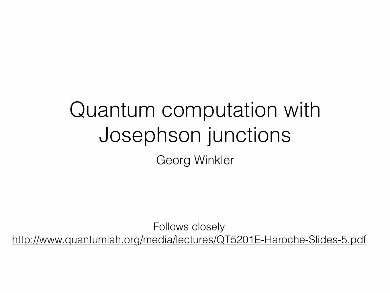
Outline

• Josephson Hamiltonian

• Quantization of Josephson Hamiltonian

• Phase qubit controlled by current

• Phase qubit controlled by flux

• Capacitive coupling of qubits

• Inductive coupling of qubits

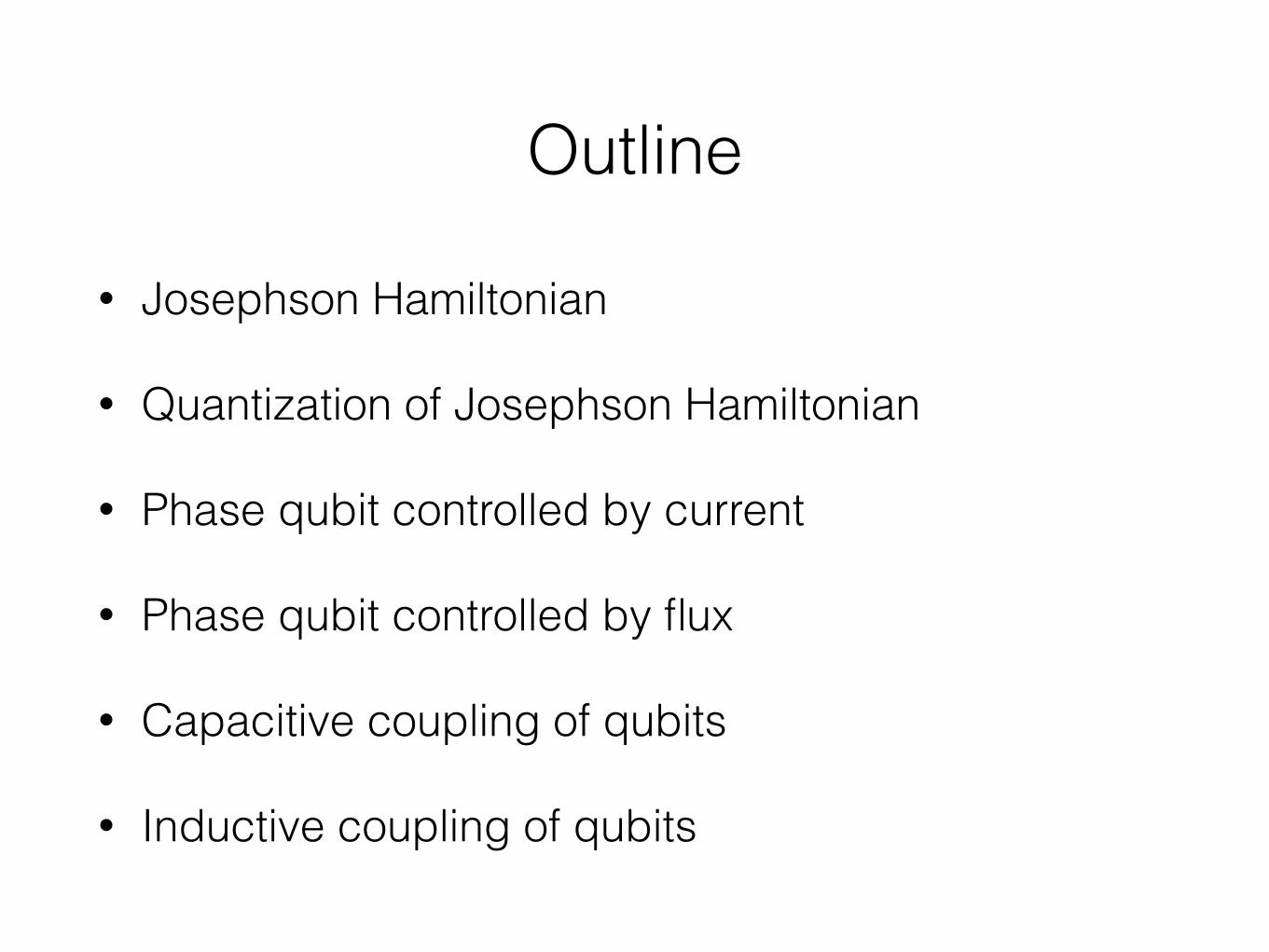
Isolated Josephson junction

• Two classical variables:

• Particle number

• Phase

• Capacity:

Description of a superconducting junction

A Josephson junction (JJ) is realized with two pieces of superconducting metalseparated by a few nanometer wide insulating barrier through which Cooper pairstunnel. When the system is isolated, we can define the number of Cooper pairs na,nband the quantum phases !a, !b of the Cooper pair wave functions on the two sides ofthe JJ. The charge and phase differences na-nb and != !b-!a are the essentialparameters describing the properties of the JJ. B.Josephson has shown in 1962that a current IJ=I0sin! circulates across the JJ without applied voltage if ! isconstant and that an ac current of frequency "= 2eV/h oscillates between the twosides if a voltage V is imposed on the JJ. These fundamental results can be derivedeither from the heuristic Ginsburg-Landau model of superconductivity, or from themore fundamental Bardeen Cooper Shrieffer (BCS) theory. They can also beunderstood by a simple model describing the ensemble of Cooper pairs as a gas ofcomposite bosons tunneling between two potential wells separated by a barrier(similar Josephson effects have been recently demonstrated in Bose-Einsteincondensates made of cold atoms).

IJ

na ,!a nb ,!b

! =!b "!a

2p = nb � na

� = �b � �a

• Josephsons equations: • DC Josephsons effect

• AC Josephsons effect

• Looks like a pendulum!

V =Q

C=

2ep

C

IJ = �2edp

dt= I0 sin �

d�

dt=

2eV

~ =4e2p

~C

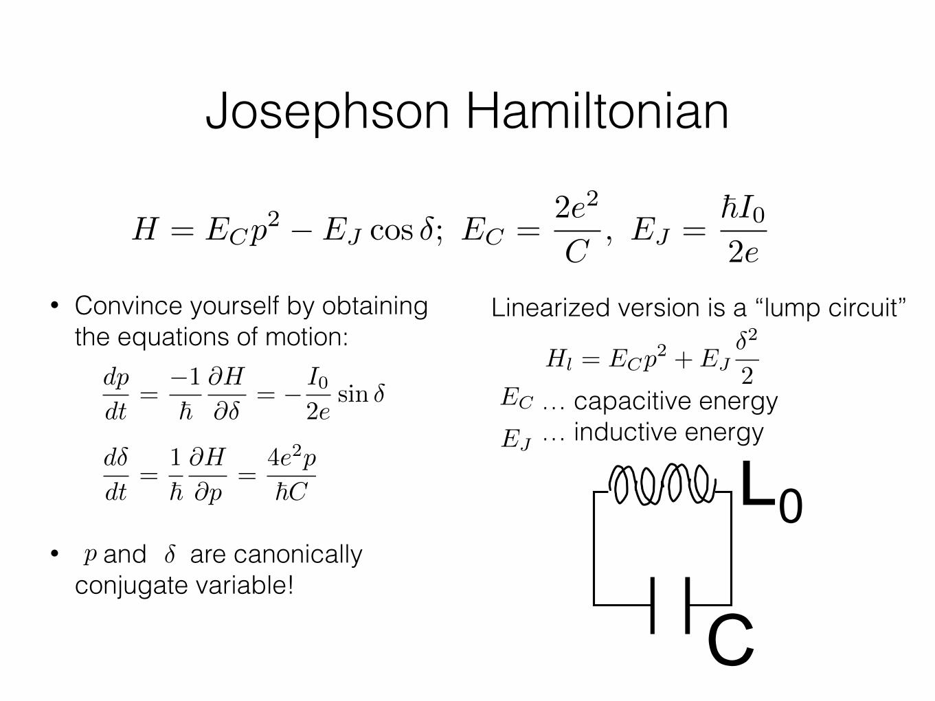
Josephson Hamiltonian

H = ECp2 � EJ cos �; EC =

2e2

C, EJ =

~I02e

• Convince yourself by obtaining the equations of motion:

• and are canonically conjugate variable!

dp

dt=

�1

~@H

@�= � I0

2esin �

d�

dt=

1

~@H

@p=

4e2p

~C

p �

Linearized version is a “lump circuit”

… capacitive energy … inductive energy

Hl = ECp2 + EJ

�2

2

The open circuit JJ HamiltonianExpressing the 2 Josephson relations as canonical eqs deriving from an Hamiltonian H, we get:

dpdt

= !I02esin" = ! 1

!#H#"

; d"dt

=4e2 p!C

=1!#H#p

$ H =2e2

Cp2 ! !I0

2ecos"

H = EC p

2 ! EJ cos" ; EC =2e2

C, EJ =

!I02e

H rules the dynamics of a non-linear oscillator whose ‘momentum’ and ‘position’ are p and !.The combined dc and ac Josephson effects induce an oscillation: a phase difference ! inducesa current (dc effect). This current produces a charge imbalance which creates, by capacitiveeffect, a potential across the JJ. This voltage induces in turn, via the ac Josephson effect, avariation of !. This produces a coupled oscillation of the phase and the charge. For small !values, such that cos! ~1-!2/2, the oscillator behaves linearly, its ‘’linearized’’ Hamiltonian Hlbeing (within an irrelevant constant):

Hl = EC p

2 + EJ!2

2=

Q2

2C+L0IJl

2

2(Q = 2ep , L0 =

!2eI0

, I jl = I0!)

This is the Hamiltonian of a classical ‘’lump circuit’’ of capacitance C and inductance L0=h/2eI0, with charge Q=2ep and current Ijl=I0!. The electric and magnetic energies of thissystem play the roles of the kinetic and potential energies of a mechanical oscillator. Making anotation change to introduce the magnetic flux #jl across the inductance, we can rewrite Hlunder a symmetrical form, where Q and #jl, proportional to p and !, are also conjugatevariables:

Hl =

Q2

2C+!Jl2

2L0; (!Jl = L0IJl =

!"2e)

C

L0

The frequency of this linearized oscillator is: !Jl =

1L0C

=2eI0!C

EC

EJ

Quantizing the Josephson Hamiltonian

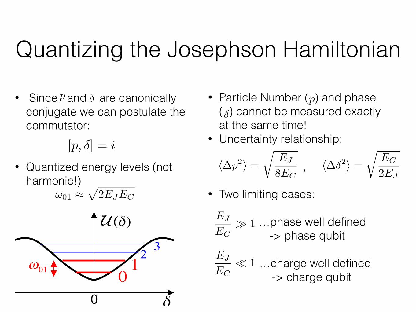
• Since and are canonically conjugate we can postulate the commutator:

• Quantized energy levels (not harmonic!)

p �

[p, �] = i

The quantized JJ realizes a qubitWhen the conjugate variables Q and # are quantized, they become non-commuting operators.The product Q# has the dimension of an action (energy x time), with the commutation rule:

which becomes equivalently for the dimentionless conjugate p and ! variables:

p,![ ] = iI

Q,!Jl[ ] = i!I

The linear L0C quantum oscillator has a ladder of equidistant levels separated by the energyh$. This equidistance is broken in the JJ system, due to the departure of the actual«potential» cos! from the !2 parabolic law: the open-circuit JJ is a non-linear oscillator.

!

U (!)

012 3

!01

Potential of the ‘’particle’’representing the JJ inopen circuit, with itseigenstates. The twolowest states 0 and 1

define a qubit.

0

Due to the breaking of the transitions degeneracy, it ispossible to manipulate with a microwave the two lowest stateswithout exciting upper levels. We thus define a qubit whosefrequency $01, close to $Jl, falls in the radiofrequency(several GHz) domain (make an order of magnitude estimateof $ with the values of e, I0 and C given above).

In fact, this open circuit qubit is not practical because it isnot controlable. We will see that by coupling it through wiresor inductances to external circuits, one can turn it into amanipulable device. Before describing practical circuits, wewill estimate the p and ! fluctuations in this very simplesystem.

• Particle Number ( ) and phase ( ) cannot be measured exactly at the same time!

• Uncertainty relationship:

,

• Two limiting cases:

…phase well defined -> phase qubit

…charge well defined -> charge qubit

p

�

h�p2i =r

EJ

8ECh��2i =

rEC

2EJ

!01 ⇡p2EJEC

EJ

EC� 1

EJ

EC⌧ 1

Realising a superconducting Qubit

Prerequisites: • controlled manipulation of qubit

without disturbing adjacent elements

• controlled inter-qubit coupling • detection of qubit state • limited influence of external

environment • sufficiently long dephasing and

decoherence times

Josephson Qubits: • Qubit Hamiltonian adjustable by

bias current and flux • State preparation via rf-Pulses • inter-qubit coupling achieved by

capacitive or inductive coupling

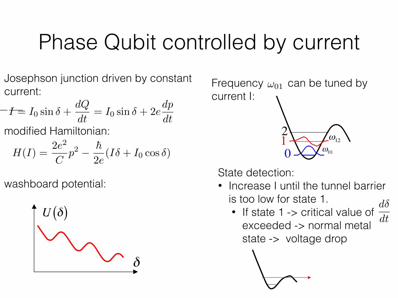
Phase Qubit controlled by currentJosephson junction driven by constant current:

modified Hamiltonian:

washboard potential:

I = I0 sin � +dQ

dt= I0 sin � + 2e

dp

dt

H(I) =2e2

Cp2 � ~

2e(I� + I0 cos �)

Josephson junction driven by constantcurrent

I I

This equation describes the acceleration of ! produced by the sum of two «forces»:The first, proportional to I0sin!, is the non-linear restoring force of the Josephsonresonator. The other, proportional to I, is an applied force imposed by the sourceof current. The sum of these forces derives from a potential proportional to- I0cos! - I !. Comparing with the Hamiltonian of the open circuit JJ, weimmediately get the current-driven Hamiltonian:

which rules the dynamics of a quantum effective particlewith conjugate coordinates ! and p in!a washboard potential.

U !( )

!

When the JJ is fed by a dc current I produced by an external source, the currentconservation in the circuit can be written by expressing the dc and ac Josephsonlaws: :

I = I0 sin! +

dQdt

= I0 sin! +CdVdt

= I0 sin! +!C2e

d 2!dt 2

(5 " 38)

H (I ) = 2e

2

Cp2 ! !

2e(I" + I0 cos") (5 ! 39)

State detection: • Increase I until the tunnel barrier

is too low for state 1. • If state 1 -> critical value of

exceeded -> normal metal state -> voltage drop

The Josephson phase qubitFor I < I0, U(!) has minima (around which it is quasi-harmonic)and maxima. Let us focus on the system’s dynamics around aminimum. The ground state and the first excited state in thepotential well associated to this minimum are separated byfrequency $01 (typically a few GHz). The second excited stateis linked to the first by a transition with frequency $12 ��$01due to the potential anharmonicity. We can thus selectivelyexcite the 0'1 transition and realize an effective two-levelsystem.

State selective detection by tunnel effect across barrier:By increasing I, we lower the barrier between two wells until wereach a configuration where state 1 has an energy just belowthe potential maximum. If the qubit is in state 1, the effectiveparticle escapes by tunneling through the barrier and !undergoes an accelerated motion down the washboard. Whend!/dt exceeds a critical value, the junction transits to thenormal phase and a voltage appears between its ports, whichgives a detection signal selectively detecting the qubit in state1. The state 0 remains stable in the well and undetected by thiseffect. In order to selectively detect 0, we can transfer thesystem from 0 to 1 by a resonant microwave pulse (see below)and then detect state 1.

012

!01

!12

d�

dt

The Josephson phase qubitFor I < I0, U(!) has minima (around which it is quasi-harmonic)and maxima. Let us focus on the system’s dynamics around aminimum. The ground state and the first excited state in thepotential well associated to this minimum are separated byfrequency $01 (typically a few GHz). The second excited stateis linked to the first by a transition with frequency $12 ��$01due to the potential anharmonicity. We can thus selectivelyexcite the 0'1 transition and realize an effective two-levelsystem.

State selective detection by tunnel effect across barrier:By increasing I, we lower the barrier between two wells until wereach a configuration where state 1 has an energy just belowthe potential maximum. If the qubit is in state 1, the effectiveparticle escapes by tunneling through the barrier and !undergoes an accelerated motion down the washboard. Whend!/dt exceeds a critical value, the junction transits to thenormal phase and a voltage appears between its ports, whichgives a detection signal selectively detecting the qubit in state1. The state 0 remains stable in the well and undetected by thiseffect. In order to selectively detect 0, we can transfer thesystem from 0 to 1 by a resonant microwave pulse (see below)and then detect state 1.

012

!01

!12

Frequency can be tuned by current I:

!01

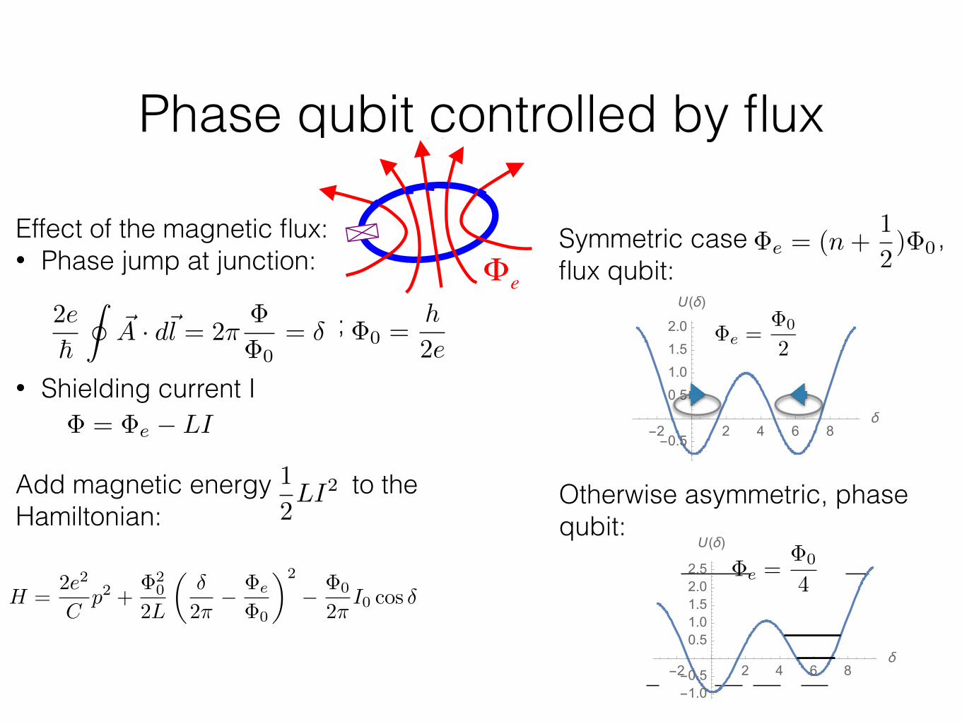
Phase qubit controlled by flux

� = �e � LI

Controlling the phase qubit by the flux

!e

MI! Instead of controlling the qubit by a dc

current, one can do it inductively bysending a magnetic flux #e across thecircuit (fig. a).

a bL

In practice, #e is produced through a superconducting dc transformer (fig. b) coupling thequbit circuit to an external one. M is their mutual inductance and L is the ‘’classical’’ self-inductance of the qubit circuit (note: do not confuse L with L0 defined above which was theintrinsic linearized inductance of the JJ). The controlling current I# produces the flux#e= M I# across the circuit qubit. An induced current I appears in L which opposes theincident flux, producing a total flux:

! =!e " LI (5 " 42)

Applying the phase quantization relation, we get the condition satisfied by the JJ phase:

! = 2" #e $ LI#0

; #0 =h2e

(5 $ 43)

which yields the expression of the magnetic energy of the L inductance versus !:

12LI 2 = !0

2

2L"2#

$!e

!0

%

&'

(

)*

2

(5 $ 44)

and leads, after adding the capacitive and intrinsic inductive contributions, to the hamiltonianof the qubit controlled by the flux #e:

H =2e2

Cp2 + !0

2

2L"2#

$!e

!0

%

&'

(

)*

2

$!0

2#I0 cos" (5 $ 45)

Effect of the magnetic flux: • Phase jump at junction:

;

• Shielding current I

Add magnetic energy to the Hamiltonian:

2e

~

I~A · d~l = 2⇡

�

�0= � �0 =

h

2e

1

2LI2

H =

2e2

Cp2 +

�

20

2L

✓�

2⇡� �e

�0

◆2

� �0

2⇡I0 cos �

Symmetric case , flux qubit:

Otherwise asymmetric, phase qubit:

�e = (n+1

2)�0

-2 2 4 6 8δ

-0.5

0.51.01.52.0

U(δ)

�e =�0

2

-2 2 4 6 8δ

-1.0-0.5

0.51.01.52.02.5

U(δ)

�e =�0

4

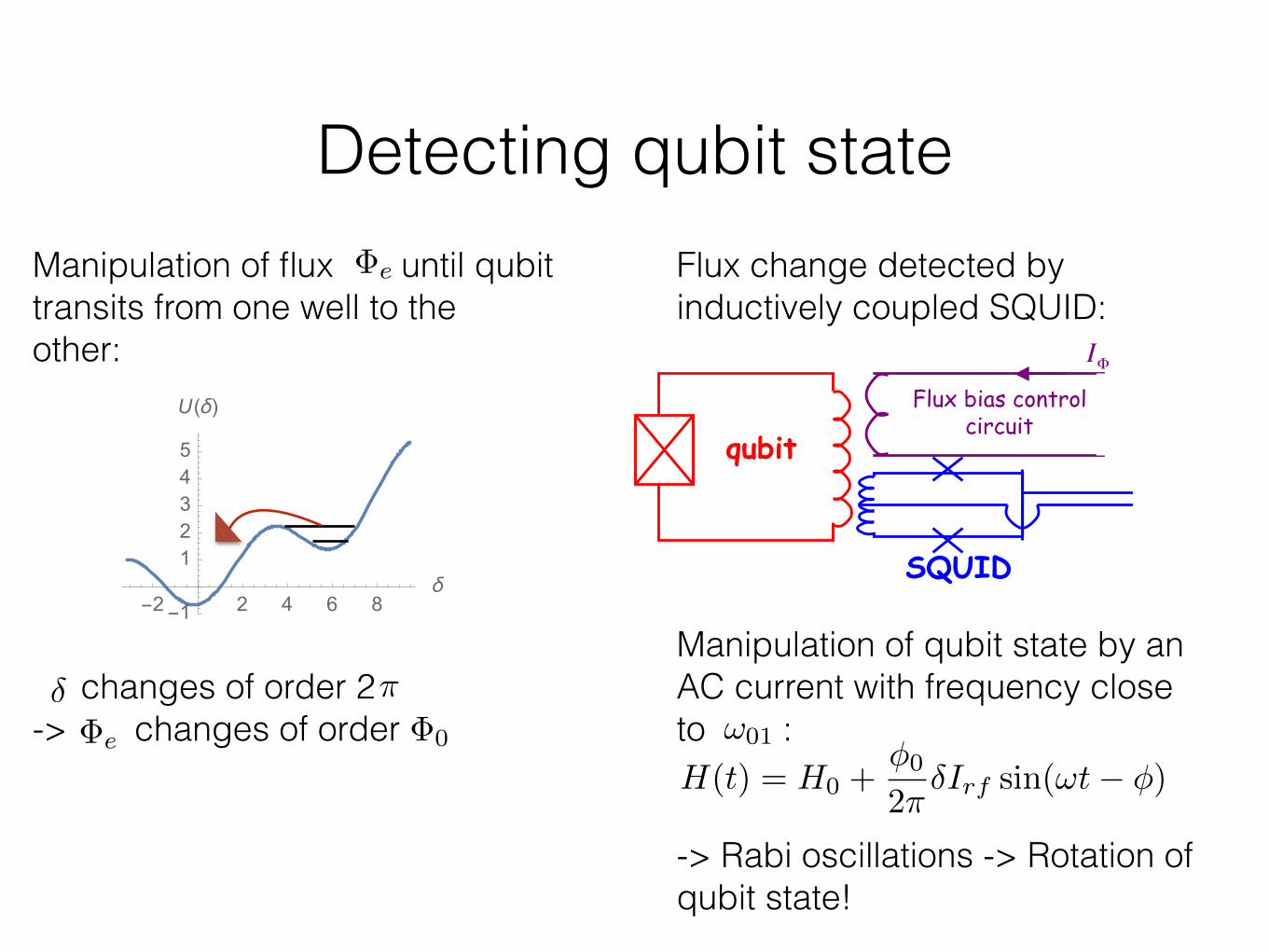
Detecting qubit stateManipulation of flux until qubit transits from one well to the other:

changes of order 2 -> changes of order

�e

-2 2 4 6 8δ

-1

12345

U(δ)

� ⇡

�e �0

Flux change detected by inductively coupled SQUID:

Manipulation of qubit state by an AC current with frequency close to :

-> Rabi oscillations -> Rotation of qubit state!

Detecting the phase qubit with a SQUIDWhen the qubit transits from one well to theother, ! changes by about %, which correspondsto a change of about I0 of the current in thequbit circuit and to a flux variation of about LI0~ #0. This sudden flux jump of about one fluxquantum is detected by a SQUID inductivelycoupled to the qubit (a voltage appears betweenthe ports of the SQUID when the qubit transitsfrom one well to the other). The flux controllingcircuit (flux bias) is used to finely tune the qubitfrequency and to bring it suddenly to thethreshold of selective detection of its quantumstates at the time of measurement.

qubit

SQUID

Flux change of theorder of #0

10

Flux bias controlcircuit

I! Sketch of thephase qubit with

its flux biascontrol circuit

and the detectingSQUID.

!01

H(t) = H0 +�0

2⇡�Irf sin(!t� �)

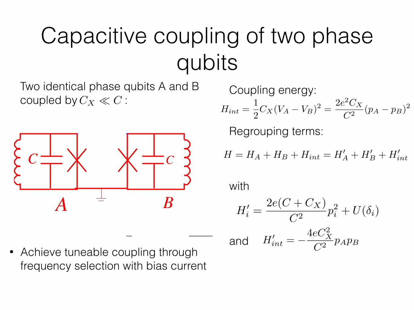
Capacitive coupling of two phase qubits

Two identical phase qubits A and B coupled by : Capacitive coupling of two qubits

CxC C

A B

The qubits «!mass!» is slighty renormalized, which modifies their commonfrequency, and a coupling term appears, which is proportional to the product of thecanonical momenta. This coupling lifts the qubit degeneracy and produces afrequency doublet in the spectrum of the coupled systems.

Consider two identical phase qubits A and B.We couple them by a capacitor whosecapacity CX is very small compared to thecapacity C of the JJ’s. The voltages VA andVB on the two sides of Cx are 2epa/C and2epb/C respectively (pa and pb are the thecanonic momenta of the two circuits). Hence,the coupling energy induced by Cx:

H int =12CX VA !VB[ ]2 =

2e2CX

C 2 pA ! pB[ ]2 (5 ! 59)

By grouping this term with the two qubit hamiltonians, we write the totalHamiltonian as:

H = HA + HB + H int = HA' + HB

' + H int'

with Hi' =2e2 (C +CX )

C 2 pi2 +U !i( ) (i = A,B) et H int

' = "4e2CX

C 2 pA pB (5 " 60)

CX ⌧ CHint =

1

2CX(VA � VB)

2 =2e2CX

C2(pA � pB)

2

H = HA +HB +Hint = H 0A +H 0

B +H 0int

H 0i =

2e(C + CX)

C2p2i + U(�i)

H 0int = �4eC2

X

C2pApB

Coupling energy:

Regrouping terms:

with

and • Achieve tuneable coupling through

frequency selection with bias current

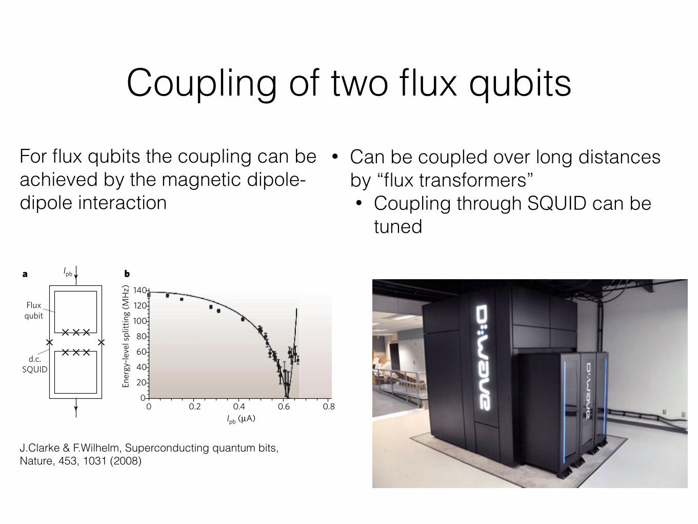
Coupling of two flux qubitsFor flux qubits the coupling can be achieved by the magnetic dipole-dipole interaction

In general, all three low-frequency processes lead to decoherence. They do not contribute to relaxation because this process requires an exchange of energy with the environment at the energy-level splitting frequency of the qubit, which is typically in the gigahertz range. How-ever, there is strong evidence that charge fluctuations are associated with the high-frequency resonators that have been observed, in particular, in phase qubits37. Improvements in the quality of the oxide layers that are used in the junctions and capacitors have resulted in large reductions in the concentration of these high-frequency resonators38.

The strategy of operating a qubit at the optimum point, which was first carried out with quantronium but is now applied to all types of super conducting qubit (except for phase qubits), has been successful at increasing phase-coherence times by large factors. Further substantial improvements have resulted from the use of charge- or flux-echo tech-niques39,40. In NMR, the spin-echo technique removes the inhomogeneous broadening that is associated with, for example, variations in magnetic field, and hence in the NMR frequency, over the sample. In the case of qubits, the variation is in the qubit energy-level splitting frequency from measurement to measurement. For some qubits, using a combination of echo techniques and optimum point operation has eliminated pure dephasing, so decoherence is limited by energy relaxation (T2* = 2T1). In general, however, the mechanisms that limit T1 are unknown, although resonators that are associated with defects may be responsible36,41. The highest reported values of T1, T2* and T2 are listed in Table 1.

Coupled qubitsAn exceedingly attractive and unique feature of solid-state qubits in general and superconducting qubits in particular is that schemes can be implemented that both couple them strongly to each other and turn off their interaction in situ by purely electronic means. Because the coupling of qubits is central to the architecture of quantum compu-ters, this subject has attracted much attention, in terms of both theory and experiment. In this section, we illustrate the principles of coupled qubits in terms of flux qubits and refer to analogous schemes for other superconducting qubits.

Because the flux qubit is a magnetic dipole, two neighbouring flux qubits are coupled by magnetic dipole–dipole interactions. The coupling

strength can be increased by having the two qubits use a common line. Even stronger coupling can be achieved by including a Josephson junc-tion in this line to increase the line’s self-inductance (equation (6), Box 1). In the case of charge and phase qubits, nearest-neighbour interactions are mediated by capacitors rather than inductors. Fixed interaction has been implemented for flux, charge and phase qubits42–45. These experi-ments show the energy levels that are expected for the superposition of two pseudospin states: namely, a ground state and three excited states; the first and second excited states may be degenerate. The entanglement of these states for two phase qubits has been shown explicitly by means of quantum-state tomography 46. The most general description (including all imperfections) of the qubit state based on the four basis states of the coupled qubits is a four-by-four array known as a density matrix. Steffen et al.46 carried out a measurement of the density matrix; they prepared a system in a particular entangled state and showed that only the correct four matrix elements were non-zero — and that their magnitude was in good agreement with theory. This experiment is a proof-of-principle demonstration of a basic function required for a quantum computer. Simple quantum gates have also been demonstrated47,48.

Two flux qubits can be coupled by flux transformers — in essence a closed loop of superconductor surrounding the qubits — enabling their interaction to be mediated over longer distances. Because the superconducting loop conserves magnetic flux, a change in the state of one qubit induces a circulating current in the loop and hence a flux in the other qubit. Flux transformers that contain Josephson junctions enable the interaction of qubits to be turned on and off in situ. One such device consists of a d.c. SQUID surrounding two flux qubits49 (Fig. 7a). The inductance between the two qubits has two components: that of the direct coupling between the qubits, and that of the coupling through the SQUID. For certain values of applied bias current (below the critical current) and flux, the self-inductance of the SQUID becomes nega-tive, so the sign of its coupling to the two qubits opposes that of the direct coupling. By choosing parameters appropriately, the inductance of the coupled qubits can be designed to be zero or even have its sign reversed. This scheme has been implemented by establishing the val-ues of SQUID flux and bias current and then using microwave manip-ulation and measuring the energy-level splitting of the first and second excited states50 (Fig. 7b). A related design — tunable flux–flux coupling mediated by an off-resonant qubit — has been demonstrated51, and tunable capacitors have been proposed for charge qubits52.

Another approach to variable coupling is to fix the coupling strength geometrically and tune it by frequency selection. As an example, we consider two magnetically coupled flux qubits biased at their degeneracy points. If each qubit is in a superposition of eigenstates, then its magnetic flux oscillates and the coupling averages to zero — unless both qubits oscillate at the same frequency, in which case the qubits are coupled. This phenomenon is analogous to the case of two pendulums coupled by a weak spring. Even if the coupling is extremely weak, the pendulums will be coupled if they oscillate in antiphase at exactly the same frequency.

Implementing this scheme is particularly straightforward for two phase qubits because their frequencies can readily be brought in and out of resonance by adjusting the bias currents37. For other types of qubit, the frequency at the degeneracy point is set by the as-fabricated param-eters, so it is inevitable that there will be variability between qubits. As a result, if the frequency difference is larger than the coupling strength, the qubit–qubit interaction cancels out at the degeneracy point. Several pulse sequences have been proposed to overcome this limitation53–55, none of which has been convincingly demonstrated as yet. The two-qubit gate demonstrations were all carried out away from the optimum point, where the frequencies can readily be matched.

On the basis of these coupling schemes, several architectures have been proposed for scaling up from two qubits to a quantum computer. The central idea of most proposals is to couple all qubits to a long central coupling element, a ‘quantum bus’56,57 (Fig. 8), and to use frequency selec-tion to determine which qubits can be coupled56–60. This scheme has been experimentally demonstrated. As couplers become longer, they become transmission lines that have electromagnetic modes. For example, two

Figure 7 | Controllably coupled flux qubits. a, Two flux qubits are shown surrounded by a d.c. SQUID. The qubit coupling strength is controlled by the pulsed bias current Ipb that is applied to the d.c. SQUID before measuring the energy-level splitting between the states !1⟩ and !2⟩. b, The filled circles show the measured energy-level splitting of the two coupled flux qubits plotted against Ipb. The solid line is the theoretical prediction, fitted for Ipb; there are no fitted parameters for the energy-level splitting. Error bars, ±1σ. (Panels reproduced, with permission, from ref. 50.)

Ipba b

00 0.2 0.4 0.6 0.8

20

40

60

80

100

120

140

Ener

gy-le

vel s

plitt

ing

(MH

z)

Ipb (µA)

Fluxqubit

d.c.SQUID

Table 1 | Highest reported values of T1, T2* and T2

Qubit T1 (μs) T2* (μs) T2 (μs) Source

Flux 4.6 1.2 9.6 Y. Nakamura, personal communication

Charge 2.0 2.0 2.0 ref. 77

Phase 0.5 0.3 0.5 J. Martinis, personal communication

1039

INSIGHT REVIEWNATURE|Vol 453|19 June 2008

• Can be coupled over long distances by “flux transformers” • Coupling through SQUID can be

tuned

J.Clarke & F.Wilhelm, Superconducting quantum bits, Nature, 453, 1031 (2008)

Conclusions and Outlook• charge and phase of Josephson junction are conjugate variables

• Frequency and detection of qubit achieved by current/flux bias

• Manipulation of qubit state by rf-pulses

• Coupled qubits can be used to create entanglement and realise quantum gates

• Decoherence can be modelled by complex impedance

• Coupling of qubit to rf LC Resonator -> Jaynes-Cummings Hamiltonian -> "Circuit QED”

Thank you for your attention.