Quantum collision theory with phase-space...
41
Quantum collision theory with phase-space distributions P. Carruthers Theoretical Division, Los Alamos National Laboratory, Los Alamos, New Mexico 87545 F. Zachariasen * California Institute of Technology, Pasadena, California 91125 Quantum-mechanical phase-space distributions, introduced by Wigner in 1932, provide an intuitive alterna- tive to the usual wave-function approach to problems in scattering and reaction theory. The aim of the present work is to collect and extend previous efforts in a unified way, emphasizing the parallels among problems in ordinary quantum theory, nuclear physics, chemical physics, and quantum field theory. The method is especially useful in providing easy reductions to classical physics and kinetic regimes under suit- able conditions. Section II, dealing in detail with potential scattering of a spinless nonrelativistic particle, provides the background for more complex problems. Following a brief description of the two-body prob- lem, the authors address the N-body problem with special attention to hierarchy closures, Boltzmann- VIasov equations, and hydrodynamic aspects. The final section sketches past and possibly future applica- tions to a wide variety of problems. CONTENTS Acknowledgments References 283 283 I. Introduction 245 II. Nonrelativistic Potential Scattering 246 A. Definitions 246 B. Equation of motion: relation to the classical limit 248 c. Integral form of the scattering equations 250 D. Exact formula for the scattering cross section 251 E. The eikonal approximation 253 F. The bound-state problem 254 G. Hydrodynamic aspects 258 H. Effect of an external potential 259 I. Gauge invariance 260 J. Spin variables 260 III. The Nonrelativistic Two-body Problem 260 A. Definitions 260 B. Equation of motion 261 c. Technical interlude: free N-particle retarded Green's functions 262 D. Equations of motiOil in the (p,q) basis 263 E. Boundary conditions 263 IV. The N-body Problem: Hierarchies and the Boltzmann- Vlasov Equation 264 A. Definitions and equation of motion 264 B. Coupled hierarchy equations for reduced distribution functions 265 c. Truncation schemes and the equa- tion 268 D. Hydrodynamic equations 273 E. Formulation in second quantization 274 F. Effect of spin and statistics 275 V. Possible Applications in Interactions of Composite Sys- terns 276 A. Composite particle scattering in the Liouville formal- ism 276 B. Models of nucleus-nucleus collisions 278 c. Atomic and molecular collisions 280 D. Solid-state physics 280 E. Second-quantization approach to inclusive reactions 280 F. Relativistic formulation of the phase-space approach to scattering and production processes 281 *On leave of absence: Los Alamos National Laboratory, Los Alamos, New Mexico 87545. Reviews of Modern Physics, Vol. 55, No.1, January 1983 I. INTRODUCTION In recent years one can discern an increasing interest in the use of quantum-mechanical phase-space distributions for the formulation and solution of scattering and produc- tion problems. These distributions, which are quantum generalizations of Boltzmann's N-particle distribution fN(PtR" ... ,pNRN,t), provide an intuitive picture of complex collision processes. As is well known (Tolman, 1938), the 6N dimensional phase space of the position coordinates qi and momenta Pi provides a useful arena for the description of classical mechanics. Quantum mechanics, which forbids states having simultaneously definite Pi and q;, requires the re- placement of the phase-space distribution function by the density "matrix" (von Neumann, 1955). An attractive version of the density matrix discovered by Szilard and Wigner (Wigner, 1932) allows the expression of quantum dynamics in a form directly comparable with the classical analog. The authors' interest in this approach occurred when they noticed that the field-theoretic formulation of inclusive production process involved second-quantized analogs of the Wigner distribution function (Carruthers and Zachariasen, 1974, 1976). In this formulation theN- particle covariant distribution functions are directly con- nected with the inclusive differential cross sections. Be- cause of the mathematical complexities of the relativistic field-theory problem, no useful predictions have yet come out of this formalism. In nuclear physics, Remler and collaborators initiated and developed a program in which nuclear reaction theory is formulated in the language of the Wigner distribution function (Remler, 1975, 1981; Remler and Sathe, 1975, 1978). Meanwhile, phase-space methods (sometimes classical) were being developed by quantum chemists in order to elucidate chemical reaction problems (Brown and Heller, 1982; Eu, 1971, 1975; Hell- er, 1976, 1977; Lee and Scully, 1980; Miles and Dahler, 1970). We hope that the present work will encourage Copyright © 1983 The Nobel Foundation 245
Transcript of Quantum collision theory with phase-space...

Quantum collision theory with phase-space distributions
P. Carruthers
Theoretical Division, Los Alamos National Laboratory, Los Alamos, New Mexico 87545
F. Zachariasen *
California Institute of Technology, Pasadena, California 91125
Quantum-mechanical phase-space distributions, introduced by Wigner in 1932, provide an intuitive alternative to the usual wave-function approach to problems in scattering and reaction theory. The aim of the present work is to collect and extend previous efforts in a unified way, emphasizing the parallels among problems in ordinary quantum theory, nuclear physics, chemical physics, and quantum field theory. The method is especially useful in providing easy reductions to classical physics and kinetic regimes under suitable conditions. Section II, dealing in detail with potential scattering of a spinless nonrelativistic particle, provides the background for more complex problems. Following a brief description of the two-body problem, the authors address the N-body problem with special attention to hierarchy closures, BoltzmannVIasov equations, and hydrodynamic aspects. The final section sketches past and possibly future applications to a wide variety of problems.
CONTENTS Acknowledgments References
283 283
I. Introduction 245 II. Nonrelativistic Potential Scattering 246
A. Definitions 246 B. Equation of motion: relation to the classical limit 248 c. Integral form of the scattering equations 250 D. Exact formula for the scattering cross section 251 E. The eikonal approximation 253 F. The bound-state problem 254 G. Hydrodynamic aspects 258 H. Effect of an external potential 259 I. Gauge invariance 260 J. Spin variables 260
III. The Nonrelativistic Two-body Problem 260 A. Definitions 260 B. Equation of motion 261 c. Technical interlude: free N-particle retarded Green's
functions 262 D. Equations of motiOil in the (p,q) basis 263 E. Boundary conditions 263
IV. The N-body Problem: Hierarchies and the Boltzmann-Vlasov Equation 264 A. Definitions and equation of motion 264 B. Coupled hierarchy equations for reduced distribution
functions 265 c. Truncation schemes and the Boltzmann~Vlasov equa-
tion 268 D. Hydrodynamic equations 273 E. Formulation in second quantization 274 F. Effect of spin and statistics 275
V. Possible Applications in Interactions of Composite Sys-terns 276 A. Composite particle scattering in the Liouville formal-
ism 276 B. Models of nucleus-nucleus collisions 278 c. Atomic and molecular collisions 280 D. Solid-state physics 280 E. Second-quantization approach to inclusive reactions 280 F. Relativistic formulation of the phase-space approach
to scattering and production processes 281
*On leave of absence: Los Alamos National Laboratory, Los Alamos, New Mexico 87545.
Reviews of Modern Physics, Vol. 55, No.1, January 1983
I. INTRODUCTION
In recent years one can discern an increasing interest in the use of quantum-mechanical phase-space distributions for the formulation and solution of scattering and production problems. These distributions, which are quantum generalizations of Boltzmann's N-particle distribution fN(PtR" ... ,pNRN,t), provide an intuitive picture of complex collision processes.
As is well known (Tolman, 1938), the 6N dimensional phase space of the position coordinates qi and momenta Pi provides a useful arena for the description of classical mechanics. Quantum mechanics, which forbids states having simultaneously definite Pi and q;, requires the replacement of the phase-space distribution function by the density "matrix" (von Neumann, 1955). An attractive version of the density matrix discovered by Szilard and Wigner (Wigner, 1932) allows the expression of quantum dynamics in a form directly comparable with the classical analog. The authors' interest in this approach occurred when they noticed that the field-theoretic formulation of inclusive production process involved second-quantized analogs of the Wigner distribution function (Carruthers and Zachariasen, 1974, 1976). In this formulation theNparticle covariant distribution functions are directly connected with the inclusive differential cross sections. Because of the mathematical complexities of the relativistic field-theory problem, no useful predictions have yet come out of this formalism. In nuclear physics, Remler and collaborators initiated and developed a program in which nuclear reaction theory is formulated in the language of the Wigner distribution function (Remler, 1975, 1981; Remler and Sathe, 1975, 1978). Meanwhile, phase-space methods (sometimes classical) were being developed by quantum chemists in order to elucidate chemical reaction problems (Brown and Heller, 1982; Eu, 1971, 1975; Heller, 1976, 1977; Lee and Scully, 1980; Miles and Dahler, 1970). We hope that the present work will encourage
Copyright © 1983 The Nobel Foundation 245

246 Carruthers and Zachariasen: Quantum collision theory with phase-space distributions
communication among these disciplines and will lead to the recognition of the phase-space method as one of universal utility.
Over the years, several authors noted the possibility of expressing potential scattering cross sections in tenns of Wigner functions (Irving and Zwanzig, 1951; Ross and Kirkwood, 1954; Mori, Oppenheim, and Ross, 1962; Huguenin, 1973; Prugoveeki, 1978a). However, the principal interest in these years was the derivation of quantum-kinetic or Boltzmann equations for uniform or almost uniform extended systems. Some other works concerned with the Boltzmann equation are Uehling and Uhlenbeck (1933); Mori and Ross (1958); Snider (1960); Snider and Sanctuary (1971); Prugoveeki (1978b). The generalization of this approach to nonrelativistic field theory and the modem formulation of the many-body problem is explained in the book by Kadanoff and Baym (1962). The most important qualitative consequence of the modem formulation is the natural manner in which "self-consistent field" theories appear in the simplest approximation. According to the nature of the system and the statistics of the particles, these approximations carry the names of Vlasov, time-dependent Hartree-Fock (TDHF), and random-phase approximation. Secondly, the transport equation can be obtained by suitable truncation of the coupled equations of motion. These techniques can be carried over to relativistic matter. One of the earliest such works, using Green's-function techniques, is that of Bezzerides and DuBois (1972). The reader is referred to the review of Hakim ( 1978) and the thesis of de Boer (1979, 1980) for further information and references on this subject.
The relation of transport equations to classical or quantum dynamics, as expressed through the coupled hierarchy of distribution functions, continues to be a problem of fundamental interest (Cohen, 1968). In this paper we shall indicate how such equations can (under suitable conditions) describe a portion of a collision process involving many particles.
Another fundamental line of investigation concerns the representation of quantum mechanics by phase-space distributions. Among the works on this topic, we mention the following: Groenewald (1946); Moyal (1949); Baker (1958); Barut (1957); Imre, Ozizmir, Rosenbaum, and Zweifel (1967); Brittin (1971); Wigner (1971); Ali and Prugovecki (1977a, 1977b); Grossman and Huguenin (1978); Prugoveeki (1978c); Balazs (1980); O'Connell and Wigner (1981a, 1981b). A review of the formalism of the Wigner function and its relation to the Weyl transformation (Weyl, 1927) has been given by de Groot and Suttorp (1972). A related topic in this area of research is the analysis of alternative definitions of distribution functions designed to satisfy special criteria (Baker, 1958; Glauber, 1963; Cohen, 1966; Agarwal and Wolf, 1968; Lax, 1968). For our purposes we do not need to worry about these fine points. In the description of inclusive scattering processes, the Wigner function arises naturally (especially in second quantization). Cross sections are directly related to it, and other issues are of secondary concern.
Rev. Mod. Phys., Vol. 55, No.1, January 1983
Recently the increased activity in heavy-ion physics has led to greater interest in phase-space distributions. Currently popular models (intranuclear cascade model, "hot spot" model, hydrodynamical models) which emphasize collective and transport behavior are especially suitable for examination in this framework. It was, in fact, our earlier interest in the Landau hydrodynamical model (Landau, 1953) of particle production which led to our search for an underlying kinetic formulation of that theory. We hope that the present work will lay the foundation for a proper description of nucleon-nucleus and nucleus-nucleus collisions. We also remark that pionnucleus scattering fits conveniently into the field-theoretic version of our formalism, with a proper (non-wavefunction) description of the pion field. References to these developments are given in Sec. VI.
The aim of the present review is to formulate in phasespace distribution language the nonrelativistic N-particle scattering of particles interacting via two-body potentials. Technical complications introduced by spin, statistics, and other degrees of freedom (e.g., isospin) will usually be suppressed. The work should be regarded as a personal essay. It is partly review and partly original, and is mostly taken from our notebooks and lecture notes dating back several years. Points of contact will be found with many of the references, however. Our main hope is to explain the lucid physical meaning of this approach to collision theory and to carry the development far enough to inspire realistic calculations. We always keep in sight the properties special to this formalism, namely, the description of collective modes and the transport and hydrodynamic behavior. Unfortunately, many of the applications will require extensive numerical work. However, that is the nature of the problems of principal interest.
II. NONRELATIVISTIC POTENTIAL SCATTERING
A. Definitions
We consider in some detail the scattering of a nonrelativistic, spinless, particle from a static potential well V. Since we are ultimately interested in the detailed spacetime evolution of complicated systems, we use wave packets throughout. The usual results can be obtained by taking suitable limits.
As is well known, one has to give up the concept of particle trajectories in quantum theory. The density of particles is expressed in terms ofthe wave function by
n (}1,t)= ll/J(J1,t) 12. (2.1)
Writing 1/J as
I d 3p. ip·B. 1/J(J1,t)= 312 C(p,t)e- ,
(21T) -(2.2)
we see that the momentum distribution implied by 1/J is
n(E_,t)= I C(E_,t) 1 2 • (2.3)
One cannot specify simultaneously the position and

Carruthers and Zachariasen: Quantum collision theory with phase-space distributions 247
momentum better than indicated by Heisenberg's uncertainty principle:
(2.4)
(Planck's constant 17 is set equal to unity except when necessary to clarify physical interpretations.)
The demise of the orbit also casts a pall on the traditional formulation of statistical mechanics in terms of distribution functions defined on phase space. The simplest of these, the one-particle function f(p,R,t), immortalized by Boltzmann, is defined so that j(p,R,t)d3R d 3p is the probability of finding a particle of momentum p and position R in the phase-space volume d 3R d 3p. The coordinate and momentum densities are, correspondingly,
n(B_,t)= J d 3pf(p_,B.,t),
n (p_,t)= J d 3Rf(p_,/l,t),
(2.5)
(2.6)
with the overall normalization taken as unity. Note that the f suitable to a single classical particle in a pure state,
f(p_,/l,t) =b(/l-/l(t) )b(p -p_(t)) (2.7)
where R(t) defines the classical orbit andp(t)=mR(t), is in direct conflict with the uncertainty principle.
Wigner (1932) has proposed a construction which both respects the rules of quantum mechanics and recaptures most of the desired features of the Boltzmann function. Notice that the density matrix (for a pure state)
(2.8)
has six c-number variables besides t. Introducing relative and center-of-mass coordinates by
r.=(~2-~d' (2.9)
/l=(~, +~2)/2'
we obtain the Wigner function by making a Fourier transform on the relative coordinate:
J d 3r -ip·r..J,* ( I )•!•( I f(p_,Jl,t) = (Z1T) 3 e - '~' 11- Tl.,t '~' /l + Tl.,t) .
(2.10)
The variable p is not an operator, but is simply a judiciously chosen-ordinary vector. It is also useful to write/ in terms of the momentum basis
d3 . f(p,/l,t)= J __!L3 e'~·Kc*(p-+q,t)C(p++q,t). - (21T) - - - -
From these definitions we see that
J d3p J<p_,Jl,t>= I 1/J<Jl,t> 12 ,
J d 3Rf(p_,/l,t)= I C(p_,t) 12 '
in analogy to Eqs. (2.5) and (2.6).
(2.11)
(2.12)
(2.13)
The function f is real, but not necessarily positive definite. The lack of assured positivity will not concern us unduly since we are mainly concerned with computation
Rev. Mod. Phys., Vol. 55, No. 1, January 1983
of positive definite asymptotic quantities like (2.13), which give the differential cross sections.
Since Eq. (2.10) is nothing but a particular representation of the density matrix, what we have is essentially the density-matrix formulation of quantum mechanics. Our approach is also closely connected with the Green'sfunction treatment of the many-body problem, as will become clear in Sec. V.E describing the second-quantization formulation of the problem. (In that section we shall consider more general density matrices.) Although the density-matrix description of quantum dynamics has little to offer in simplicity for easy problems involving only a few particles, it really comes into its own for complex, many-particle dynamics. We shall argue that the Wigner version, suitably generalized, is the most natural way to formulate and solve such problems.
The simplest example is a free particle,
C (p,t) = C (p) exp(- ip 2t /2m) , - - 3 (2.14)
J d q +iq·(R-v t) I I fo<p_,/l,t)= (Z1T) 3 e - =-e C*(p_- 2 q)C(p_+ 2 q),
where !2p =p_ /m. For a wave packet made up of free particles, / 0 depends on 11 as /l-Qt. The example of the Gaussian momentum packet (peaked at p 0 and R 0 ) is especially useful and interesting,
exp[ -(p -p0 )2/4u] . C(p_)= (21Tu)3/4 exp( -zp_·/lo)' (2.15)
exp[ -(p -p0 )2/2u] fo(p_,/l,t)= (21Tu)3/2
exp[ -(R -R0 vpt)2 12L] X (21TL)3/2
(2.16)
where L is defined by L = 1/4u. We point out some interesting features of Eq. (2.16):
(a) It does not spread with time for fixed p, even though the underlying wave function does. However, contours of constant f, described by a generalized ellipse, do spread in the phase plane.
(b) The momentum and position distributions obey the uncertainty relation ll.px!::..Rx ~ T· Hence an equation like (2.7) is out of reach, except as a special limit involving 17---+0.
(c) As L tends to infinity f 0 becomes spread uniformly over space, while the momentum factor is sharp in momentum.
The Gaussian packet (2.16) is an especially good prototype incident-free packet. Since we shall use these results for large L, the normalizations appropriate to the continuum counterparts are listed (as L---+ oo ):
(L)314C(p_)---+b(p_-p_0 ),
(L/21T)314t/lp0 (/l)---+exp[ip_o(/l-/lo)] ,
(L /21T)312f 0 (p_,/l,t)---+b(p_ -p_0 )/(21T)3 •
(2.17)
The indicated continuum normalization is 1/(21T)3 parti-cles per unit volume.

248 Carruthers and Zachariasen: Quantum collision theory with phase-space distributions
Other examples of analytically calculable phase-space distributions will be given in Sec. II.F.
Before taking up the question of computing j(p,R,t), we explain how to express the result of a scattering experiment in the present formalism. We imagine (Fig. 1) a nearly uniform wave packet with momentum components p ~Po incident on a localized potential V. The extent of the packet L 112 needs to be much larger than the size of the potential (called a) if we use Eq. (2.16) as our prototype packet. (Figure 1 has been drawn for R 0 equal to zero; for L- oo, the memory of R 0 disappears from the problem.) After the incident packet scatters off V, the outgoing signal is detected in the solid angle dfl (Fig. 2). As time tends to infinity all particles pass by the detector. We rewrite Eq. (2.1) in differential form, giving
dNscatt I 3 --3-= d Rj(p,B.,t lt--->oo.
dp -(2.18)
To calculate the incident flux and consequently the cross section, we note that the probability current is
j(!i,t)=-21 . (t/J*V.,P-V.,P*t/1)
- mz
(2.19)
the latter following an easy calculation. Therefore, the incident integrated flux along the beam direction Po is
dNinc I"" . A ---;u-= ""dtJ_o'Pofo(p,R,t). (2.20)
Using Eq. (2.14) for fo and noting that in the limit of sharp wave packets!!.. ~l!..o• q ~o, we can derive
dNinc I 3 I 3 A I ---;u-= d p d q[)(q_·vo)C*(J!..-Tq)
XC(p+-}q)/(27d.
The differential cross section is then
I d 3Rj(p,R, 00)
dNincldA
(2.21)
(2.22)
In this form one can take the continuum limit. Note that
0 FIG. 1. A smooth free-particle Wigner distribution with momenta peaked near J!.o approaching a localized potential V.
Rev. Mod. Phys., Vol. 55, No.1, January 1983
since our f includes the incident particles, the definition (2.22) does not agree with the traditional one in the forward direction p 0 • This question will be clarified in Sec. II. E.
B. Equation of motion: relation to the classical limit
The equation of motion for f follows directly from the Schrodinger equation,
i ap(R,t) = [ - V2 + V(R) ]·'·(R t) . (2.23) at 2m - 'I'_,
The result is more complicated formally, involving essentially the commutator of H with the density matrix. But this form is directly related to the Poisson bracket form of classical mechanics, as shown below.
The kinetic term is most easily computed in momentum basis, giving
I d3q eiq·R [ (J!..+-}q_)2- (J!..--}q_>2]c*( _2.. t) (27T)3 2m 2m !!.. 2q_,
1 ip XC(p+ 2 q,t)=- ~VRf(p,R,t). (2.24)
- - m -
The full equation of motion is then
.!2[_= [~+v ·V l/(p R t) Dt at "4' -·-·
=-1- I ~e-ie_·r.I"[V(R 2..r)-V(R-2..r)] ifz (27Tfz)3 -- + 2- - 2
(2.25)
We have temporarily reinstated the correct factors of fz in order to facilitate our discussion of the classical limit. Equation (2.25) can be usefully rewritten as
FIG. 2. The outgoing particle's density in phase space. This allows the evaluation of the cross section d u in the solid angle dO.

Carruthers and Zachariasen: Quantum collision theory with phase-space distributions 249
[ V(E. + T!.)- V(E.- T_r)Jf(p',E_,t) (2.26)
= f d 3p' K(p_' -p_,E.)/(p_',/i,t) ,
where the function K,
K(p'-p R)=-1- J ~ei<e.'-e.l!:.HI[ V(R+2.r) - _,_ ifz (21rli)3 - 2-
- V(R _2-r)] - 2
(2.27)
occurs in many of our calculations. We shall also use the Fourier transform
iK(p'-p,q)= V(q)[ fJ(p'-p +Tq)
-fJ(p' -p- +q>J . (2.28)
The difference of potentials occurring in Eq. (2.27) is important only for r ;Sa, where a is the range of the potential. Hence the significant momentum differences p_' -p_ occurring inK are of order lp_' -p_ I _:Sfz/a. Therefore, in the equation of motion (2.26), the potential has the effect of connecting f 's with p' in the range p' ~p±fz/a. The finite contributions for r = ±2R ±a oscillate if R >>a and do not contribute for short-range potentials.
In the classical limit, (2.26) becomes local in momentum space, too. In the limit fz---+0, expanding
V(R +112r)-V(R -1/2r)~r·VV
and writing r =iVp/fz leads to the classical one-particle Liouville equation,
Hence Eq. (2.26) may be regarded as a quantum Liouville equation. Information on classical scattering theory in the phase-space language can be found in Prigogine (1959) as well as in Miles and Dahler (1970) and Eu (1971, 1973).
Equation (2.29) is equivalent to the constancy of the phase-space density (df /dt =0), provided the particles move on classical orbits specified by Newton's laws: dr.!dt =p /m, dp !dt =- VV. The solution is then f[p(t),r.fi)]. -
ff we keep all terms in the expansion of V, we easily derive
[ ;t +v·V k(p,R,t)
(ifz)n-1 = ~ n- 1 1 (Vp·VR)nV(R)j(p,R,t)
nodd 2 n.
=~sin [ fzVp;VR ] V(R)f(p,R,t). (2.30)
Here and subsequently it is understood that V R acts only
Rev. Mod. Phys., Vol. 55, No.1, January 1983
on V. The form (2.30) is most easily derived by writing
V(/i± 1!2r.)=exp( ± l/2V)V
in Eq. (2.27), which leads to
2 [fzV ·VR K(p'-p,R>=-,;sin P2 ] V(R)fJ(p'-p).
(2.31)
In either the quantum case [Eq. (2.26)] or the classical case [Eq. (2.29)] the motion is ballistic in the absence of a scattering potential. More precisely, the equation
..Q.f= [~+v ·V ]/=0 (2.32) Dt at >qJ
is solved by any function of R -12pt. The initial condition for the scattering problem is of this form.
The differential operator occurring in Eqs. (2.29) and (2.30) has the form
If we expand f formally in a power series in fz,
f=fo+fzf1+fz2fz+ · · · ,
we find the sequence of equations
[~~-Do ko=O, [ ~~ -D0 k1 =0,
[ ~~ -Do k2 =Dzfo ,
[ ~~ -Do k3 =Dz/1 ,
[~~-Do k4=Dzfz +D4fo,
[ ~~ -Do ks =Dz/3 +D4f1 .
(2.33)
(2.34)
(2.35)
These equations are solved in sequence by simply integrating along the classical orbits, keeping in mind the initial distributions, whose fz content will vary with the problem. For example, having found / 0 , we calculate / 2 from the equation
/ 2 =/~0 l + J~,., dt'(Dzf0 )[p(t'),r(t')] . (2.36)
In this manner the entire quantum distribution is constructed in terms of the underlying classical orbits.
When the boundary condition is independent of fz, only even powers of fz occur in the formal series (2.34). One of the first applications of the quantum phase-space distribution (Wigner, 1932) was the calculation of quantum corrections to the Boltzmann distribution. Although such results seem to make sense for thermally averaged quanti-

250 Carruthers and Zachariasen: Quantum collision theory with phase-space distributions
ties, the formal expansion does not exist (Heller, 1976) in many important cases. The reason is that essential singularities spoil the expansion of Eqs. (2.34). A very simple example is the free Gaussian distribution, Eq. (2.16), in which the fi dependence is of the form h 3 exp( -A /fi2 ).
Hence every Vp brings in factors fi- 1 and fi- 2, canceling factors of fi in the expansion (2.34). We refer the reader to the work of Heller (1976) for further information as well as for the description of a method to explicitly extract the singularities responsible for the failure of the naive approach outlined above. The essence of his method is to remove the essential singularities through a selective summation of the infinite series in fi. The problem is sufficiently important to deserve further study.
The phase-space distribution method has been used to illustrate various features of the (tricky) classical limit. The reader is referred to the following authors for further information and references: Heller (1977); Berry (1977); Berry and Balazs (1979); Berry, Balazs, Tabor, and Voros (1979). Particularly interesting is the semiclassical (WKB-derived) phase-space distribution derived and studied by Berry (1977). We expect that further development of these ideas for scattering theory will lead to important practical applications.
It is instructive to note that we can easily prove an "Ehrenfest theorem" using the Wigner distribution
d(p > = I d3 d3R at<p,/i,tl =-vv. dt P !!.. at
(2.37)
A similar calculation for (E.) leads directly to
d(/i) = {p_)
dt m (2.38)
For these simple moments, the classical procedure of computing expectation values coincides with the usual quantum-mechanical rules. For discussion of the generality of this, one should consult the references.
C. Integral form of the scattering equations
As is usual in scattering theory, it is useful to formally integrate the equation of motion to exhibit the incoming boundary condition explicitly. In anticipation of our later development, we pose the problem not only for j(p,R,t), but for the corresponding space and time Fourier transforms.
Consider the equations
[ ;t +.!!.·V ]t(p_,/i,t)=S(p_,/i,t),
[i ;t -q·.!!. )tcp_,q_,tl=iS(p_,q_,tl, (2.39)
(w-q_·.!!.)/(p_,q_,w)=iS(p_,q_,w),
where
f( )- I d3 -i•rB.J< p_,q_,t = R e f!..,/i,t) ,
/(p_,q_,w)=. I d3R dt eimt-i'1_·B.f(p_,/i,t) '
with analogous expressions for the transforms of S. The Green's functions corresponding to Eqs.
obey
[ ;t +.!!.·V ]G(p_,/i,t)=6(/i)6(t),
[i ;t -q_·Q ]G(p_,q_,t)=iB(t),
(w-q_·Q)G(p_,q_,w)=i.
(2.40)
(2.39)
(2.41)
As usual, one has to define the pole suitable to the desired boundary condition (here retarded). The result is
i G ret(p,q,w) = . '
w+ze-q_·Q
Gre1(p,q,t)=it(t)e-iq·vt, (2.42)
when {t(t) is the usual step function: unity for t > 0 and zero for t < 0.
The integral forms of Eq. (2.36) are evidently
j(p,/i,t)= f 0 (p_,/i,t)
+ I~"" dt'S[p_,Ji -Yp(t -t'),t'] '
f(p_,q_,t) = fo(p_,q_,t) (2.43)
I t -iq·v.(t -t') + -co dt'e _, S(p_,q_,t'),
iS (p,q ,w) f(p,q,w)=fo(p,q,w)+ . . -- -- w+ze-q_·Q
Here f 0 solves the homogeneous equation suitable to the three descriptions: as t---+- oo, f---+ f 0 • The retardation factors, which have an obvious physical meaning, find differing expression in the three forms of Eq. (2.39). Applying these results to the equation of motion (2.26) leads to the scattering integral equation
f(p_,/i,t)= fo(p_,/i,t)
+It dt'd 3p'K[p'-p,R-v (t-t')] -oo P
Xf[p',Ji -Yp(t -t'),t'] . (2.44)
Physically, it is clear that the values of f at retarded points build up the whole function. The kinematicalkinetic content of Eq. (2.44) is exposed by iterating. To illustrate, the second-order term is
t t' I dt' I dt" I d 3p' I d 3p"K[p' -p,R -v (t -t')]K[p" -p',R -v (t -t')-v' (t' -t")] -oo -oo P P P
xJ[p",R -vP(t -t')-v; (t' -t"),t"] . (2.45)
Rev. Mod. Phys., Vol. 55, No. 1, January 1983

Carruthers and Zachariasen: Quantum collision theory with phase-space distributions 251
Pictorially [Fig. 3(a)] the particle density begins at timet", is deflected from p" top', propagating with velocity v; until t', when the potential changes the momentum top. Then the density propagates between t' and t with velocity vP.
In nth order we have
In (dtid 3pi)K(p2-Pt>RI) ... K(p,. -Pn-i>R,.)f(p,.,R,.,t,.)' (2.46) i=i
where the variables are given by
R 1 =R -vp1Bti> Bt1 =t -t' ,
The physical interpretation is again suggested by Fig. 3(b). For many purposes the (q,w) language is convenient. The scattering integral equation is
f(p,q,w)=fo(p,q,w)+ . 1 I (d23q)'3 V(q')[f(p-+q',q-q',w)-f(p++q',q-q',w)],
w+LE-q_·~ 1T (2.47)
where the incoming distribution function is
fo(p,q,w)=21TB(w-q_·~)C*(p -+q)C(p ++q). (2.48)
It is easy to show that the differential cross section is the residue of a pole inf(p,q,w) at w=O for q_=O. For f!_=/=-f!_o we have
(2.49)
It is instructive, though tedious, to solve Eq. (2.44) by iteration,
f=fo+f1+h+ · · · ,
where
1 d 3 , fn+l(p,q,w)= . I~ V(q')[f,.(p -+q',q -q',w)-j,.(p ++q',q -q',w)].
-- w+zE-q_·~ (21T) (2.50)
'
Note that since fo exhausts the normalization we have
I f,.(p,R,t)d 3p d 3R =0, n;:;::: 1 . (2.51)
f 1 does not contribute to the cross section as anticipated (it is linear in V). Working through the details, one finds the flux factor (2.21) explicitly, giving in second order
v d3u =(27T)-2 1 V(p -pol I 2B(E -Eo) · dp - -
(2.52)
Rather than derive this explicitly, we shall show how our formalism leads to the general formula wherein the Born cross section (2.52) is replaced by the identical formula with V replaced by the transition matrix. Our calculation is somewhat similar to that of Gottfried ( 1966), who uses the density matrix.
D. Exact formula for the scattering cross section
In order to derive the generalization (2.48), we begin by expressing the Fourier transform of (2.11) in Dirac's bracket notation,
f(l!_,q_,t)=C(f!_ + Tq_,t)C* (f!_- Tq_,t)
=<l!_++q I 1/l(t))(l/l(t) IP -+q>. (2.53)
The wave function 1/1 obeys the usual equation
Rev. Mod. Phys., Vol. 55, No. 1, January 1983
1/l(t)=cp(t)-i I~"' dt'e -iHo<t-t'lVt/l(t'), (2.54)
where 1/1-cp as t-- oo and the exponential oscillations are to be tamed by the adiabatic hypothesis. We can ex-
(Rn-2!n-2l Pn-1
FIG. 3. Iterative contributions to the scattering integral equation. (a) The structure of the second-order iterate [Eq. (2.45)]. The retardation terms propagate the phase-space densities freely between interactions with the potential. (b) The structure of the nth-order iterate.

252 Carruthers and Zachariasen: Quantum collision theory with phase-space distributions
pand 1/J and cp in terms of the stationary wave functions exp(ik·.!.) and 1/Jt(,!.), respectively, using the same expansion coefficient X(p):
( ) J d 3p X( )eiE:lf-iE , qJ ,!.,t = (21T)3/2 !!_ p '
(2.55)
·'·(x_,t)= J d3p X(p)·'·+(x)e-iEp' 'I' (21T)3/2 - 'l'p - '
where Ep=p 2!2m. For a sharp X(p)=(21T) 312fj(p--k), we find the usual result
1/Jt(,!.)=eih+ .1 V!/Jt(x) . (2.56) Ek+1e-H0
The usual transition matrix for scattering from momentum state k to k' is
(2.57)
In our calculations it will be useful to use the related amplitude
Tp(t)= (p I vI 1/J(t) >
(2.58)
Here we have labeled X with a momentum p 0 , about which we shall eventually make Xp0 (k) peak. The equa-
tion of motion is
[i :t -llp·q_ k(p_,q_,t)=(p ++q I vI 1/J(t)}(!/J(t) IP -+q )-(p ++q I 1/J(t)}(!/J(t) I v IP -+q>. (2.59)
As it stands, Eq. (2.59) exhibits only one explicit Von the right-hand side. But the desired structure, containing two V's and two 1/J's, results immediately on substituting the integral equation (2.50), converting the right-hand side of Eq. (2.59) to:
(p + +q I v I 1/J >< cp I P - +q > - (p + +q I cp >< 1/J I v I P - +q >
+i(p + Tq IV I 1/J(t)) J~ .. dt' exp[iEp-q;2(t -t')]( 1/J(t' I VIP- Tq)
+i J~ .. dt'exp[-iEp+q/2(t-t')](p+Tq I VI!/J(t'))(!/J(t}l Vlp-+q). (2.60)
The first two terms are nonzero only in the forward direction p 0 for q =0 and will be dropped here. The time integrals in the third and fourth terms are evaluated using Eq. (2.55). Further performing the time Fourier transform gives
J d 3kd 3k' 21T 3 Xp0(k)X; (k')6(w+Ek·-Ek)
(21T) 0
X [ Ek-E:+:12-ie + Ek·-Ep~q12 +ie X(p++q I Vl1f!t><1f!tl Vlp-+q>. (2.61)
Making the substitutions k=P+Q/2, k'=P-Q/2, we can express Eq. (2.59) in the form
J d 3Pd:Q X*(£-+Q)X<E+TQ)6(w+E·Q/m) (21T) - - -
[ 1 1
X EP-QI2-Ep-ql2+ie - EE.+Qn-Ep-q/2-ie
X(p++q I VI!/JP+Q/2)(1/Jt-Q/21 Vlp-+q>.
(2.62)
We are interested in the limit of this expression for q_=w=O and for the wave-packet coefficients Xp0 sharply
peaked around p0 • This allows us to set Q =0, p =Po in slowly varying functions. Hence for p_ol=p_o we find -
Rev. Mod. Phys., Vol. 55, No.1, January 1983
-i[wj(p_,Q,w)].,=o=21Tfj(EPo-EP) I (pI VI 1/J"Jo) 12
X f d3Pd3Q X*(P-2.Q) (21T)3 2
XX(P + TQ)f)(P·Q!m) .
(2.63)
Recognizing .the flux factor from Eq. (2.21) and using (2.49) leads directly to
v d3a =(21T)-2fj(E -Eo) I (p IV I 1/J"J) 12' (2.64) dp 0
where v =p0 /m is the incident velocity. We now clarify the special features of the wave in
terference behavior in the forward direction and in so doing show how the optical theorem arises in the present formalism. · Our previous definition of the cross section (2.22) was unorthodox in counting all final particles, including the incident beam. This approach is too tied to the classical approach and obscures the important phenomenon of diffraction scattering.
To clarify this question, we note that corresponding to the decomposition
(2.65)
to which (2.54) tends as t---+ oo, we have for the Wigner distribution

Carruthers and Zachariasen: Quantum collision theory with phase-space distributions 253
/=/o+/int+fsc • (2.66)
where / 0 , lint• and /sc are, respectively, the incident, interference, and scattered components. In the equation of motion / 0 drops out. In Eq. (2.60) the first two terms dropped are exactly the interference terms which arise from the overlap of the incident and scattered wave. Therefore, the necessary correction to Eq. (2.22) is the subtraction not only of the fo contribution (exactly as in classical mechanics), but also of the interference term. From Eq. (2.60) we see that this interference term is just the imaginary part of the T matrix, as one should expect, in the limit q ~0.
The continuum limit of Eq. (2.60) is easy to take. In that limit the various states become energy-momentum
E. The eikonal approximation
eigenstates and the left-hand side vanishes as q---+-0. The vanishing of the right-hand side then produces the optical theorem as a constraint. From Eq. (2.56) we see that a suitable normalization for continuum states is (2'7T)3l>(e' -e>· Performing the trivial time integrations gives
(21T)3li(e-eo>[(p IT IPo)-(p IT IPo>*J
+21Tili(E -Eo> I TPPo 12=0 . (2.67)
Integration over d 3p gives the usual form,
High-energy, small-angle potential scattering is well described by the eikonal approximation (Glauber, 1959). This result can be easily derived in the present formalism by one simple approximation, i.e., replacing the velocity in the drift term v·V by the incoming velocity v0 =p0 /m.
We write the equation of motion in the form (2.26)
. [a ] J d 3rd 3p' i(n'-p)·r I I z at+v0 ·V j(p,R,t)= (21Ti e "" - [V(B.+-rr>-VCB.--rr)]/(p',R,t).
Noting the convolution structure in momentum, we can rewrite this in terms of
j(y,R,t)= J ~e1l!.'lj(p,B_,t) (217") -
as
i [ :t +vo·V k(y,R,t)=[V(R +fy>- V(R -fy)]/(y,R,t).
[Note that the exact equation corresponds to replacing v0 by -iVy in Eq. (2.71).] Equation (2.71) is solved by integration,
f(y,R,t)=fo(y,R,t)exp [ -i f~oo dt'{ V[R +TY -v0 (t -t')]- V[R -fy -v0 (t -t')]}] ,
(2.69)
(2.70)
(2.71)
(2.72)
where / 0 is as usual the incoming density function, transformed as in Eq. (2.66). Therefore, the desired phase-space density is
/(p,R,t)= J d 3y e-ip·yfo(y,R,t)exp [ -i J~oo dt'{ V[R + TY -v0 (t -t')]- V[R- TY -vo(t -t')]} ) . (2.73)
Defining variables parallel and perpendicular to v0 in the obvious way and writing z =R 11 -v0 (t -t') allows us to rewrite Eq. (2.73) as
/(p,R,t)= J d 3y e -lp·yf0 (y,R,t) exp { ~oi J~~ dz [ V [z + Yii ,R1 + y; ] - V [z- Yii ,R1 - y21 ] ] } • (2.74)
Now all the time dependence has been placed in an especially simple, controllable function, namely, the free motion described by / 0 .
We now use the Gaussian / 0 of Eq. (2.16) to simplify (2.74). We find, setting R 0 =0,
. -CR -u0t> 212L J(y R t)=-1-e'Po'Ye-uy212...:..e ____ _
' ' (217")3 (21TL)312 (2.75)
where eventually we shall want to take the limits a---+-0, L---+- oo. To obtain the cross section, we need to integrate Eq. (2.74) over Rand study the behavior as tot---+- oo. To accommodate the structure of the potential term, it is use-
Rev. Mod. Phys., Vol. 55, No.1, January 1983
ful to change variables as follows:
I Yt=R +-rY,
I Y2=R --rY ·
Further writing
Yt 11 =Zl>Yl =lzt ,
Y2 11 =z2,Y21 =l2.2
(the b1 will be impact parameters), we obtain after a little arithmetic

254 Carruthers and Zachariasen: Quantum collision theory with phase-space distributions
f d 3Rf(p,R,t)= f d 2htd2b2exp[-i(p-p0 )1 ·(b 1-b2)]exp l- [ bt:b2 rt-L j
Xexp[ -u(bt -b2 )2 /2] f dz1dz2 exp[ -i(p -po)II(Zt -z2)] exp l- [ 21 : 22 -v0 t r;2L j
where the function <I> is defined by
[ i Jzl l <l>(z,b)=exp -- dz V(z,b) Vo -oo
(2.77)
The complex expression (2.79) simplifies greatly in the limit t---+ oo, since then the only contributions come from z 1 +z2 ---+oo,too. Actually,z1 andz2 tend to +oo together for finite u because of the factor exp[ -u(z1 -z2 )2 /2]. For finite-range potentials <l>(z,b)=<l>( oo,b) as soon as z exceeds the potential range. Hence the Zt>Zz dependence of the potential functions <I> disappears as t---+ oo . Going over to coordinates z =z 1 -z2 , Z =(z 1 +z2 )/2, we can do the two integrations explicitly,
-(Z-v0t)2!2L
f dZe J dze-(u/2)z2e -(P-Polllz (21TL)I12
;:::;21TI>(pi!-Po);:::;21Tvoi>(E -Eo)'
reinterpreting the u---+0 integral as an energy-conserving delta function.
Letting u---+0, L---+ oo inside the fl. integrations, we find
f d 3Rj(p,R,oo)= 21L - 1- 3 21Tvoi>(E-E0 )
1T (21T)
X I J d2b e -l4:11<1>( oo ,fl.) 12 '
(2.78)
where fl=p -p0 is the momentum transfer. The coefficient 1/(21TL) is nothing but the flux factor
(2.20) evaluated for the Gaussian as L ---+ oo :
[ dN J 2 1 -d =exp( -R 1 /2L)/21TL---+-- . A 21TL
Finally, writing
d 3p =p 2 dp dE dn dE
and integrating over E gives
(2.79)
du = l_p_ J d2be-il:..-bexp [--i J"" V(Z,b)dZll2 dfl 21T v0 -oo
(2.80)
This formula differs from the usual one by the absence of a - l accompanying the exponential. The - l comes from subtracting the incident wave to define a scattered amplitude. Our formalism, which involves the full J, includes everything, and therefore the definition (2.22) does
Rev. Mod. Phys., Vol. 55, No.1, January 1983
(2.76)
not coincide with the traditional definition of the cross section in exactly the forward direction. That is, of course, where the discrepancy lies, in that the - 1 term produces a I)(Jl) on performing the b integration. Equation (2.80) involves the full J, while squaring <I> -1 leads to an immediate identification with the terms in Eq. (2.66).
F. The bound-state problem
In the preceding sections we have formulated the quantum scattering problem in terms of the time-dependent solutions to the Liouville equation
Lf=iaf at '
(2.81)
where the quantum Liouville operator L is defined by
L (p,R )/ (p,R, t) = - ivp · "i1 Rf (p,R, t)
+if d 3p'K(p' -p,R)j(p',R,t).
(2.82)
For energy eigenstates, t/Jn -e -iE.tf is time independent, so that Inn constructed from such wave functions must satisfy
Lfnn=O · (2.83)
It might be imagined that Eq. (2.84) is a combined eigenfunction-eigenvalue problem for En and the associated phase-space distributions. It turns out that, in contrast to the scattering problem (for which the boundary conditions are different), the Liouville equation does not determine the Wigner function in this case.
A first indication of this comes from a closer inspection of the equation of motion (2.45) in the case when f has no explicit time dependence. For bound states there is, in addition, no incident wave packet. Shifting variables to r=t' -t gives the bound-state equation
0 fB(p,R)= J -oo dr J d 3p'K(p_' -p_,B. +12prl
X/(p_',B. -12pr) . (2.84)
In Fourier transform language this becomes
q·!lpfB(p,q)= f dV3 V(q')[fB(p ++q',q -q') - (21T)
-fB(p- +q',q -q')]
(2.85)

Carruthers and Zachariasen: Quantum collision theory with phase-space distributions 255
in agreement with Eq. (2.47) adapted to bound states. To illuminate this equation further, we rederive Eq. (2.85) from the bound-state Schrooinger equation in momentum space:
[E- ..£.__2 2 ]X(q)= f dq' 3 V(q')X(q -q') , (2.86) m (21T)
where the X's are defined (and called C) in Eq. (2.2). From Eq. (2.11), we find for f(p,q)
I I j(p,q)=X*(p --zq)X(p +-zq). (2.87)
We now constructj(p,q) in two ways usipg Eq. (2.86):
(E -Ep_912 )X*(p --}q)X(p +fq>
f __!}ff__ I I = 3 V(q')X*(p--zq+q')X(p+-zq), (21T) (2.88)
I I (E -Ep+q12 lX*(p --zq)X(p +-zq)
= f __!}ff__ V(q')X*(p- ...!...q)X(p + ...!...q -q'). (21T)3 2 2
Identifying the integrands as j(p + -}q',q -q') and j(p- -}q',q -q') and subtracting gives Eq. (2.85), since
Ep+qi2-Ep-ql2=p-q/m .
The cancellation of the energy eigenvalue in going from Eq. (2.88) to Eq. (2.85) leads to the suspicion that the latter may not, in general, determine the energies or eigenfunctions of the bound states. This is in contrast to Eq. (2.86), which poses a standard eigenvalue-eigenfunction problem.
In order to clarify this situation, we note that the basic equation of motion (2.81) is a particular realization of the density-matrix equation of motion
i*=[H,p]. (2.89)
As a consequence, the solution to the more general eigenvalue problem
(2.90)
(A. real but not necessarily positive) is easily surmised by inspection of Eq. (2.91). Writing Pmn = I m) (n I, where I n ) , I m ) represent energy eigepstates, we see that
.aPmn z-,.-=(Em-E,lpm, ·
ot (2.91)
Recalling the relation between the density matrix and the Wigner distribution [Eq. (2.10)], we see that the eigenfunctions of L corresponding to Eq. (2.91) are the offdiagonal generalization off:
~" ( >-J d 3r -te:r..'·"'( 1 ) Jmn p,R,t = --3 e .,.,, R --zr,t. . (21T)
I Xt/Jm(R +-zr,t),
Lfmn=(Em-EII)fmn •
I" ( )- -i(Em-En)tl" (0) Jmlt t -e Jmn •
Rev. Mod. Phys., Vol. 55, No.1, January 1983
(2.92)
where the phase-space integral of f m11 vanishes. We now see that the energy eigenvalues are to be constructed from the eigenvalue spectrum of L.
Since the Pmn form a complete set of matrices by which any operator can be represented, so do the f mn of Eq. (2.92) form a complete set. In particular, a general f can be represented as
f(p,R,t)= ~ Cm,fm,.(p,R,t). (2.93) mn
It is useful to state here the completeness and orthogonality conditions obeyed by the f mil. (For this purpose, we remove the time dependence of the energy eigenstates.) Straightforward calculations using the completeness and orthogonality of the wave functions lead to
(2.94)
~fm,(p,R)j;,,.(p',R')=B(R -R')B(p -p')/(21T)3 . mn
In the particularly interesting case when the system is subjected to an external potential Vex CB., t ), the Cm, 's become time dependent and induce transitions among the various "stationary" solutions f mn (cf. Sec. II.H).
The construction (2.92) provides the desired solution to Eq. (2.90). However, an attempt to solve (2.90) does not lead uniquely to Eq. (2.92). A symptom of this difficulty is easily seen from the form of the density-matrix analog to Eq. (2.90):
(2.95)
Clearly any solution to this equation can be multiplied by an arbitrary function of the constants of the motion without changing the eigenvalues.
The problem evidently is that the single equation (2.90) is not completely equivalent to the Schrodinger equation. The proper resolution of this situation has been clearly laid out in a recent paper by Dahl (1981). In addition to the commutator structure Lf++[H,p ], we need the anticommutator analog .LJ~-}[H,p]+, with the associated eigenvalue problem
(2.96)
Clearly we can reconstruct the usual Schrooinger eigenvalue problem from L and L. The (p,R) form for L is easily obtained by suitably changing signs in Eqs. (2.24) and (2.25). Noting that f mn also solves Eq. (2.96),
we find for the kinetic energy term
I L 1 2 -z[T,p]+-+ 2mfm,- 8m VRfmn ·
(2.97)
(2.98)
Combining this with the potential energy term, we find

256 Carruthers and Zachariasen: Quantum collision theory with phase-space distributions
+ f d3p 1K(p~-p,R)tmn<P 1,R),
(2.99)
where the kernel K is given by
K( ~- R)=.2.. J ~ei(p'-p)·r p p, 2 (21d
X[V(R +Tr)+V(R -+r)].
(2.100)
Note that the time dependence of tmn cancels out in Eq. (2.99).
Equations (2.90) and (2.99) provide the required constraints to solve the eigenvalue-eigenfunction (matrix) problem. Note that tmn will have to vanish for r~oo, p ~ oo if m and n are both bound states. In the continuum, of course, the eigenvalue is arbitrary and Eq. (2.91) suffices to determine the solution to the scattering problem.
If we expand in r.., we find
K = V(R )B(p 1 -p)- .2.. V:.'!(R )__E_ __E_B(p 1 -p) + ... s 'J apj apj
(2.101)
Note that the leading term is just
[£ l I Hclass(p,R)tmn= 2m +V(R) tmn=-:z(Em+E,.)tmn'
(2.102)
the classical equation of motion, whose energy is the average of the two quantum energies.
In order to demonstrate this and other points, we examine the one-dimensional harmonic oscillator. In coordinate space, the stationary Liouville equation is
_i!__E__t(p,x)=i J dp 1K(p 1 -p,x)t(p 1,x), m ax
where for V = +mw2x 2, the kernel simplifies to
iK(p' -p,x)=mw2x aa B(p 1-p) . . lfJ
t therefore must satisfy
at =(mw)2 at . ax2 ap 2
(2.103)
(2.104)
(2.105)
For our discussion of the oscillator, it is useful to express x and p in units of the zero-point motion values x 0 and p0 • x~ is (2mw)- 1, while x 0p0 =+ defines p 0 • These values correspond to the minimum uncertainty character of the ground-state wave function
Rev. Mod. Phys., Vol. 55, No.1, January 1983
1 2 2 ¢0(x)= 114 112 exp( -x /4x 0 ). (21T) x 0
(2.106)
From this wave function, we easily compute the Wigner function
t<p,x)= 1 exp(-x 2/2x~-p 2/2p~), (2.107) 21TXoPo
which is (not surprisingly) a joint Gaussian in p,x. Noting that (mw)2 =p~/x~, we write Eq. (2.96) in the form
at at a(x/xo)2 = a(p/p~) . (2.108)
Clearly the ground-state result (2.108) satisfies this condition, but so does any Gaussian exp[ -A (x 12 +p 12 )], where the prime denotes the natural dimensionless variables x/x,p/p0 •
Writing the energy in these units,
H(p,x)=+w(p' 2 +x 12 ),
we can easily confirm from Eq. (2.107) that
E 0 = J dpdxH(p,x)t(p,x)=+w,
(2.109)
(2.110)
but the differential equation (2.108) does not determine t<p,x), and so the ground-state energy is correspondingly undetermined.
Next we see that the more general equation (2.83) does give the energy eigenvalues, even though the t mn are not uniquely determined.
Using Eq. (2.104) for the oscillator kernel, we can write the Liouville operator in the form
L . [ I a I a ] =lW X apl -p ax' . (2.111)
As in the classical case, the Liouville operator acts as a rotation in the phase plane. Naturally, H (or the action, classically) commutes with L. Introducing action angle variables in the phase plane as in Fig. 4,
x =J coscp,
p =Jsincp,
where J 2 is proportional to H, we find
H= const
(2.112)
FIG. 4. The harmonic oscillator phase plane. The condition H = const defines a circle in the phase plane, when p and x are normalized to their zero-point values.

Carruthers and Zachariasen: Quantum collision theory with phase-space distributions 257
L =iliJ_E_ . acp (2.113)
Hence the single-valued eigenfunctions and eigenvalues are
fn =e-incp' (2.114)
An =nliJ, n =0, ± 1, ±2, ...
These fn may, of course, be multiplied by an arbitrary function of the action J, without changing An.
To determine the f mn we may supplement the foregoing with Eq. (2.99). For the oscillator the expansion (2.101) terminates after the second term, giving
[L mliJ2 _1_ [Jt... m2liJ2v2] ]1 2m + 2 - 8m ax 2 + P mn
I =-z(Em+En>fmn. (2.115)
Dahl (1981) points out that the equation is identical to the two-dimensional oscillator Schrodinger problem. The solutions are in terms of the generalized Laguerre polynomials L:;',
I" =N ex (-_!_S)·S(I/2)In;-nji.L ln;-nji(S) J njni m;nj P 2 n
(2.116)
where n is the greater of n;,n1 and the other variables are defined by
S = _i_Hclass =(p'2 +X'2 ) • li)
1 _ 1 n 1 _ 1 n' r= --tan __r__ = --tan ~ ,
liJ m liJX liJ X
r n/ j 1/2
1 (n;!)3 N;i = --;; 2 e ifliJ
(2.117)
with b;1 an arbitrary phase. x',p' are the dimensionless variables defined following Eq. (2.100). For the usual
ifl.. R· choice of phases e '1 = ( -1) '. The result (2.116) general-izes earlier results found by Groenewald ( 1946), Uhlhorn (1956), Heller (1976), and Takabayashi (1954). (Dahl has 2 in place of 1 hr in Nil; we have changed to conform to our convention that 11= 1.)
The ease of obtaining explicit f mn for the onedimensional oscillator allows us to illustrate several further points. First of all, from our previous analysis we know that the functions of fno computed from the correct wave functions must be proportional to the eigenfunctions fn -e -inrp of the Liouville operator. For example, explicit calculation gives
fw=(x'-ip')j00 (p',x')a::e-irp, (2.118)
in agreement with Eq. (2.117). As mentioned earlier, the Wigner distribution for
bound states typically becomes negative in some regions of phase space. Let us examine the definition (2.10) for
Rev. Mod. Phys., Vol. 55, No. 1, January 1983
bound states to understand better where negativity will occur. First of all, the variable R has to be in the potential well for 1{1 to be large; r cannot exceed the range a in the integration. The more highly excited the state, the more nodes in the wave function and the greater the probability of negative values. For r -a, we can expect significant negative contributions so long as p < 1/a, i.e., wavelengths of the order of or larger than the potential range. For sufficiently large p, the exponential oscillation restricts r to small values so that the overlap becomes positive. Hence, for R in the potential, we can expect negative values off whenever p < 1/a.
A nice example of these qualitative remarks is given by the first excited state of the oscillator, 1{11 a::x1{10(x). An elementary calculation yields
ill (p,x)= 21T;oXo (x'2+p'2-l )exp(- +x•2_ TP'2) .
(2.119)
The circle x'2 +p'2 = 1 divides phase space into domains of positivity and negativity. As claimed, we need x in the well (x' < 1) and sufficiently small p to reach the negative, nonclassical domain for / 11 • For general n, Eq. (2.116) specializes to the simple form
(2.120)
where Ln is the ordinary Laguerre polynomial and f 00 is defined in Eq. (2.107). The domains of negativity are clearly annuli (Fig. 5) in the x'p' phase plane, since the Ln
+ +
x/x 0
+ +
(o)
+ +
(b)
{c)
FIG. 5. Domains of positivity of the Wigner distribution for the first three excited states of the one-dimensional harmonic oscillator. For the first excited state, f 11 is negative within the unit circle. For the second state, the inner circle is positive, followed by an annulus where f 22 is negative, and finally a positive region. For large enough action fnn is always positive. The annulus structure reflects the simple properties of the Laguerre polynomial of Eq. (2.120).

258 Carruthers and Zachariasen: Quantum collision theory with phase-space distributions
have n real zeros. The signs are such that Inn is positive for large values of the argument.
Finally, we note two especially useful Wigner distributions involving the harmonic oscillator. The first corresponds to the density matrix for thermal equilibrium,
p=exp( -/3H)/Trexp( -/3H) . (2.121)
The phase-space distribution for this has been computed by Davies and Davies (1975) to be
1 I l(p,x)= -tanh ( 2/3w)
1T
X exp[- +<p'2+x'2)tanh ( +/3w)] . (2.122)
The second example concerns the coherent state I a) (Glauber, 1963); Carruthers and Nieto, 1965, 1968)
p=la)(al,
la(t))=e-<112llal2 f an(t: In)' n=O Vn.
(x la)=t/Ja(X)
(2.123)
- \ 114 exp[-(x-(x) 2/2x~+i(p)x], (21Tx 0 )
where a(t)=ae-i"'t. The phase-space distribution is
l(p,x,t)= 2 1 exp{ -[x -x(t)]2/2x~
1TXoPo -[p -p(t)]2/2p~} (2.124)
Hence I is distributed in a Gaussian manner about the classical motion, in faithful correspondence to the intuitive interpretation of the coherent state.
In each of these cases, which involve summation over the excited oscillator states, I is positive throughout phase space. The negative-valued regions, which are uninterpretable classically, correspond to bound-state problems. The motion of the center of mass, however, is described by an essentially smooth positive phase-space distribution.
Phase-space plots of l(p,x) for the first four energy levels of the one-dimensional square-well potential may be found in the work of Baker, McCarthy, and Porter (1960). In the case of a linear potential, one gets an Airy function, as discussed by Heller (1977) and Dahl (1981).
From these examples and the general discussion, it is clear that bound-state wave functions typically (except for the ground state) give regions of negativity. This is in contrast to the scattering problem, where sufficiently smooth packets give rise to positive joint distributions like the Gaussian packet, Eq. (2.16). In any case, the cross section arises from the positive quantity (2.13). Similarly, the cross section for the production of a many-body bound state is given by an expression like Eq. (2.13), with the internal variables (and negative phase-space regions) integrated out.
G. Hydrodynamic aspects
It was found very early (Madelung, 1926) that Schrodinger's equation could be recast as a hydrodynamic
Rev. Mod. Phys., Vol. 55, No.1, January 1983
pair of equations (continuity and an Euler equation for irrotational flow). Writing tf!=a exp(i/3), (a,/3 real), we note that the probability current is
j_=a2V/3/m , (2.125)
so that we can identify the velocity as
!:J.=V/3/m. (2.126)
This suggests that /3/m plays the role of a velocity potential cp.
The same current, obeying the usual conservation law,
an v. 0 -+ ']= at -
(2.127)
(n =a2), is obtained as the imaginary part of the Schrodinger equation in the (a,/3) variables. The real part can be identified with the (irrotational) Euler equation.
We now explore the hydrodynamical connection in the context of the Wigner distribution, beginning with the equation of motion (2.26).
Integration over d 3p gives immediately
an -+V·(nu)=O at •
where local average velocity !:J.(R,t) is defined by
I d3p Jdpl<p.R >.t> u(R,t)= I - d3p l<e.R.,t>
(2.128)
(2.129)
(vp =elm). The potential term disappears, since I d 3p produces a B(z:.) under the d 3r integral.
The analog of Newton's law follows on taking the first moment
nu; =I d 3p vp,f<e.R..t)
in the equation of motion,
a a I 3 -a (nu; >+-a d p vp.vpj(p,R,t) t Xj I
=I d 3p d 3p'K(p' -p,R)vp,f(p',R,t)
1 =--(V;V>n,
m
(2.130)
(2.131)
the latter form following on using the explicit form for K. We compare this with the usual momentum equation of
continuum hydrodynamics,
a a -a (pu;>+-a-T;k=O, t Xk
(2.132)
T;k=pu;uk+B;kP, (2.133)
where pis the mass density and p the pressure. We now see that the stress tensor for the Schrodinger equation is
Tfk =p( V;Vk > +Bijp• ,
Vp•=nVV,
I d 3p vpj(p,R,t) ( V;Vk) = -=----'---
I d 3p l(p,R,t)
(2.134)
(2.135)
(2.136)

Carruthers and Zachariasen: Quantum collision theory with phase-space distributions 259
Equation (2.136) involves the correlation (v1vk ), in contrast to the uncorrelated velocities u1uk in Eq. (2.133). By reexpressing (2.136) in terms of uncorrelated velocities, we make contact with the usual Euler equation.
Making use of the identity
(v1vk)=:((v1 -u1 )(vk-uk))+u1uk, (2.137)
we rewrite (2.131) as
a a a -a (putl+-a (putuk)=-nVV--a-Pti, t xk xk
(2.138)
where the kinetic pressure tensor is given by
I d 3p(v1 -u1 )(vk-uk)f(p,R,t)
Ptk =p I d3p f(p,R,t) (2.139)
Expanding derivatives on the left-hand side and using current conservation reduces Eq. (2.138) to Euler's equation
P [ a:rt +.«·Vut] = -p v::- a:i Pti , (2.140)
when -pV1 V /m is the external force density. Similar considerations have been discussed by Kan and Griffin (1977).
H. Effect of an external potential
Our discussion so far has dealt with pure scattering or bound-state problems. In the presence of a timedependent external potential, we can excite bound states (either to other bound states or to the continuum) or can
induce "capture" of the free particle into a bound state. In principle, these processes are symmetrical, but the usual experimental arrangement leads to a somewhat different treatment.
Corresponding to the choice of potential energy,
V(R)+ Vex(R,t) , (2.141)
we write the basic equation of motion as
[ :t +v·V ]t(p,R,t)- I d 3p'K(p'-p,R)f(p',R,t)
=I d 3p'Kex(p'-p,R,t)j(p',R,t) . (2.142)
For an initial bound state, Eq. (2.44) no longer holds, since fn does not obey the homogeneous equation, but instead
~Jn(p',R,t)- I d 3p'K(p'-p,R)fn(p',R,t)=0.
(2.143)
Of course, the ti~e dependence actually goes away, as discussed in Sec. II.F. In addition, Eq. (2.143) does not determine f B.
In order to solve Eq. (2.142), we clearly need the interacting Green's function
i]!_G(p,R,t)-i I d 3p'K(p'-p,R)G(p',R,t) Dt
=8(_e)8(£)8(t) (2.144)
subject to suitable boundary conditions. For example, the Wigner function for an initial bound state satisfies
f(p,R,t)=fn+ I~oo dt' I d 3p' I d 3R'Gret(p'-p,R',t')Kex(p'-p,R',t')j(p',R',t'). (2.145)
If the initial particle is free, we can still use Eq. (2.54) with K +Kex replacing K. In this case, the final state will contain both bound-state and continuum components. Since the wave function can be written as an expansion in energy eigenfunctions as
1/1= l:an..Pn+ I d 3kC(khpt, (2.146) B
only energy-degenerate cross terms survive in the timeaveraged Wigner function. In particular, the contribution of the final bound state B (assuming no accidental degeneracy) is ian 1 2/nn. as expected.
The explicit calculation of the retarded Green's function obeying Eq. (2.144) is usually quite complicated. We content ourselves with expressing G in terms of the "eigenmatrices" f mn of the Liouville operator [of Eq. (2.93)]. Introducing the Fourier transform G(p,R,co) obeying
(L -co )G (p,R,co) = 8(_e )8(£) ,
and expanding G = l: Gmnf mn gives
l: Cm,.(Am11 -co)/m11 (p,R)=8(p)8(R). mn
Rev. Mod. Phys., Vol. 55, No. 1, January 1983
(2.147)
(2.148)
The orthogonality relation (2.93) is now used to evaluate Cmn• giving
G ( R )- ~ .t:,,(O,O)/m11 (p,R) R p,_,co - ~ , .
- mn "'mn -co+l£ (2.149)
when the ie is added to enforce the right boundary condition in the continuum.
Many commonly occurring problems, e.g., excitation through interaction with an external system, are conveniently modeled by the introduction of an external potential energy Vex(~,t). The total Hamiltonian is then H r = T + V + Vex• and it is natural to express the evolution of the phase-space distribution in terms of the f mn referred to the Hamiltonian T + V of the system being perturbed. We therefore write the expansion
f(t)= l: Cm,(t)fmn(t), (2.150) mn
where the Cmn depend on time by virtue of Vex. The f mn form a complete set, though the orthonormality relations are not very simple.
The expansion coefficients are exactly those of the density matrix. For a pure state, we have

260 Carruthers and Zachariasen: Quantum collision theory with phase-space distributions
p= 1~><~1
m,n mn (2.151)
m
where Pmn = I m ) ( n I is the same as occurred in Eq. (2.56).
Beginning with this result, one can do time-dependent perturbation theory in the standard manner by writing
c -c<o>+A.c< 0 +A.2c<2>+ ... mn- mn mn mn (2.152)
(where Vex is of order A.). We then obtain the set of coupled iterative equations
;cw>=o, •• (I) - (0) - (0) lCmn = ~ ( V mk Ckn - Vkn Cmk) • (2.153)
k
.'(2) - (I)- (I) lCmn= ~(VmkCkm-VkmCmk) ·
k
By normalization the diagonal C's must obey the constraint
~Cmm=1. (2.154) m
These results can be applied to nondegenerate groundstate excitation in the standard way. For A.=O, C~1=BmoBno· If t<O, Vex=O and C~~(t<0)=0. The c:..On remain constant in time.
1. Gauge invariance
In the presence of external electromagnetic potentials, it is necessary to modify the definition (2.10) in order to obtain a gauge-invariant phase-space distribution function. Under a gauge transformation the potentials transform like
A'=A +VX, qJ'=qJ-! ~~ . (2.155)
The form of the Schrodinger equation is unchanged when the wave function transforms as
(2.156)
From this it is clear that the integrand of Eq. (2.10) requires modification by a path-dependent phase factor
I' I d 3r -tp·r Jp(p,R,t)= --3 e -(21T)
(2.157)
where the line integral runs along a path P beginning at B.- fc. and ending at B.+ fc..
In a simply connected region, the loop integral of A will vanish and the particular path P makes no difference.
Rev. Mod. Phys., Vol. 55, No.1, January 1983
For multiply connected domains, such as are encountered in the Aharonov-Bohm experiment, the phase factor becomes crucial.
The distribution (2.157) has an equation of motion whose classical limit is the one-particle Liouville equation (2.28) when the force term - VV is replaced by the usual Lorentz force (de Groot and Suttorp, 1972; BialynickiBirula, 1977).
J. Spin variables
We note briefly the extensions required to describe the spin variable in the most important case of spin f. Letting a,b denote the z component of the spin, we define a 2 X 2 matrix Wigner function f with elements
- I ~ -te·c..,.* ..!... ) fab(p,R,t)- 3 e 'f'b(R- 2 r,t (21T)
The ordinary density is then
j(p,R,t)=Trf
(2.158)
- I ~ -ip·r.,,,*(R _!__ )·'·( _!__ ) - 3 e - '~' - 2 r,t '~' R + 2 r,t . (21T)
(2.159)
The reality of f for the spinless case is now replaced by Hermiticity f+ =f, i.e.,
(2.160)
Such an f can be represented by two independent functions/a and/1 and a real unit vector fi'as follows:
f=fo+rz:fi'f1 · (2.161)
The polarization density can be computed from the expectation value of the spin operator as follows:
Q:.(e_,B.,t) = Tr(Q:.f)
I d 3r -ip-r t 1 1 = (21T)3 e - '1/J (R - 2r,t)Q:.~(R + -zr,t) .
(2.162)
We can express the ordinary and spin densities in terms of / 0 and/1 as follows:
j(e_,Ji,t)=2fo(P,R,t) ,
Q:.(e_,Ji,t)=2fi'/l(E_,B.,t).
(2.163)
(2.164)
Ill. THE NONRELATIVISTIC TWO-BODY PROBLEM
A. Definitions
The two-body problem exhibits in simplified form some of the kinematical features of the N-body system. Of

Carruthers and Zachariasen: Quantum collision theory with phase-space distributions 261
course, one recovers the one-body problem in the absence of external potentials when the two-body potential depends on the distance between the particles. Until the final parts of this section, we treat the problem of two spinless, distinguishable particles of the same mass, with Hamiltonian
PT p~ H= 2m+ 2m +vC!:t-,!.z)+Vt(,!.l>t)+V2 (,!. 2,t).
(3.1)
The external potentials V; act on the ith particle. We have in mind two classes of problems:
(1) scattering of particles 1 and 2, (2) breakup of a bound state by external potentials.
The V; are imagined to have a finite extent in space. An example of case (2) is the photodisintegration of the deuteron, where particle 1 is a proton, particle 2 a deuteron, while V1 represents an external electric potential and V2
vanishes. In order to generalize Eq. (2.10), we again take the
Fourier transform on the relative coordinates xj -xl> xi -x2 in the density matrix 'll*(xl>x2 )'11(xj ,xi). Making the definitions
I ' R I ,!.t=Rt-271> ,!.t=-t+2!.t'
we define the two-particle distribution to be
/z(p_t .Rt ,p_2,R2,tl
=I
(3.2)
(3.3)
Expanding in momentum basis, we have the alternative form
(3.4)
B. Equation of motion
FIG. 6. Kinematical space variables suitable for the twoparticle distribution [see Eq. (3.3)]. The x;,x; label the split points of the wave function. R 1, R 2 tum out to be the effective locations of particles 1 and 2, while R=+(R 1+R 2 ) and r = R 1 - R 2 have the usual significance of total and relative coordinates.
Although / 2 itself need not be positive definite, the joint momentum and coordinate distributions are, as expected,
I d 3ptd 3P2f2(/?_1Rt>f.2/?_2t)= I 'II(R!>R2t) 1 2 ' (3.5)
I d 3Rtd 3R2f2(/?_tRI>/?_2R2t)= I C(p_!>/?_2,t) 1 2 .
As suggested by the notation, (p;,R;) have the significance of the position and momentum variables in the kinematical phase space.
Our analysis will require additional position variables defined by Fig. 6:
- I e.=c.t -l.z, R = 2(!.1 +1:2) • (3.6)
1 , , 1 ,!.J-,!.2=c.-2e.• ,!.t -,!.2 =c.+2e. ·
As suggested by the notation, (R,r) are the em and relative coordinates. In addition, we shall require total and relative momenta,
I p_=e_t +p_2, /?_=2(/?_t-/?_2),
PT p~ L +P2 I -+-= -- (p=-m, M=2m). 2m 2m 2p 2M 2
(3.7)
The two-particle Boltzmann drift term can then be expressed as
(3.8) v=(pt-P2)/m, V=f.IM.
A similar decomposition can be made for particles of unequal mass.
The equation of motion for / 2 is derived in direct analogy to the one-particle case. We find
[ ;t +.ll.t"Vt +11.2"V2 k2(/?_I>Rt/?_2R2t)= I d 3pjd 3p2K2(p_j -e_te_i -p_2,RtR2)/2(PiRtP2R2t)
+I d 3piKt(P't -e_t,Rt,tl/2(p_!Rt/?_2R2t)
+ I d 3p2Kt(e_i -p_2,R2t)/2(/?_IRte_iR2t)'
Rev. Mod. Phys .• Vol. 55, No.1, January 1963
(3.9)

262 Carruthers and Zachariasen: Quantum collision theory with phase-space distributions
where v1 isp1/m, V1 is a;aR1, etc. The kernels K1 are defined exactly as in the one-body problem except that the potentials V1,2 can be time dependent. The kernel K 2comes from the interparticle potential
. , , _ J 2 d 3rj t<ej -I!.J>·rj 2_ 2_ 2_ _2. ] zK2(PI-PttP2 -p2,RttR2>= II --3 e [v(RI + 2l.1.R2+ 21:2)-v(B,.I- 2l..R2 2l.2) ·
- - - - J=l (21T)
K 2 simplifies greatly by virtue of v depending only on the relative coordinate. After a suitable change of variables, we find
I d 3R d 3p - I - I I I iK2(pj -p1,pi -p2,Rt.R2)= 6 exp[i(pj -p1HR +Tp)+i(pi. -p2HR -Tp)][v(r +Tp)-v(r -2p)]
(21T)
=B(pj +pi -PI-P2) J ~exp[i(p'-p)·p][v(r++p)-v(r-1-p>] (21T)
which is independent of R. The kernel conserves overall momentum (an expression of translation invariance), while the action of the potential is determined by the relative variables. In the presence of external potentials, the overall space-time translation invariance is lost, and energy and momentum can be exchanged with the two-body system.
We now demonstrate in detail the separation of the center-of-mass and relative motion starting from Eq. (3.9). The assumed wave function is
[ ~I +~2 ] 'I' =X 2 ,t <1>(~1 -~2,t) . (3.11)
X is a wave packet representing the center-of-mass motion of the form of Eq. (2.2) with Cas in Eq. (2.14), and with P the total em momentum peaked around P 0 • An elementary calculations leads to the phase-space distribution
fz <e1 R 1 .1!.28.2 t)
[ R1+R2 l [Pt-P2 l =/o l!.t +e2 2 ,t I 2 ,Rt-R2,t '
(3.12)
where fo is the free-packet function of Eq. (2.14) and f, given by
_ J ..!!.!.e._ -trern. *( 2. )m.( 2. ) f(l!_,[.,t)- (211")3 e - "¥ l.- 2p,t "¥ r.+ 2p,t '
(3.13)
is time independent for the case of an energy eigenstate. Note that /o is a function of R-Et, as expected. Therefore, a;at + V·V R gives zero when acting on / 0 , so that the left-hand side of Eq. (3.9) becomes
(3.14)
To see that /o also factors out of the right-hand side, we use Eq. (3.10) to simplify. Noting that the Jacobian is unity on going from {p 1,p2)--"'(J!.,p), we find
Rev. Mod. Phys., Vol. 55, No.1, January 1983
(3.10)
d 3P'd 3p' J (211")3 8(P' -P)K 1 (p' -p,r)j0 (P',R,t)f(p',r,t)
! fl._ , , =fo(P,R,t) (21T)3 K 1(p -p,r)f(p ,r,t).
(3.15)
Hence the relative motion is described by the one-body equation of motion with K, and calculated from the potential v (r). Note that the factorization occurs independently of the shape of the em wave packet.
C. Technical interlude: free N-particle retarded Green's functions
In order to cast the equation of motion in integral form suitable for scattering problems, we need the generalization of the retarded Green's function to two and more particles.
Consider the defining equation for N particles,
DG Dt (l!_tRI · · 'l!_N&tl=B<Rtl8(B,.2 ) • • • 8(IiN)8(t),
D a N -=-+ ~.!l;·V;. Dt at i=l
Writing Gas a Fourier transform,
N d3qi G<etRt · · ·eN&t>= f II~
j=l (21T)
gives the equation
(3.16)
(3.17)
(3.18)
[i :t- f ~·.!!.1 ]G(l!_t~J.t · · 'l!_Nq_Nt)=i8(t) . (3.19) j=l
Finally, transforming in time gives

Carruthers and Zachariasen: Quantum collision theory with phase-space distributions 263
(3.20) G(p,q, ... PNqN{J))= +. ~ ' -- - - {J) .1€- ~j 9_j'Jl.j
where the i E has been added to enforce a retarded boun-dary condition.
In R,t variables, we find easily
aR<ed!., · · · eN&tl =-3(t)BCB. 1-Q1t)B(B.2 -Q2 t) · · · B<&-QJft).
(3.21)
an intuitive result whose correctness can be verified directly.
In passing, we note another intuitive but important result,
D -F(R ·-V·t)=O. Dt _, _, (3.22)
=-3(t)exp( -i 1: q.]"ll.Jt) • (3.23) j
D. Equations of motion in the (p,q) basis
It is often convenient to rewrite the formalism by carrying out Fourier transforms on the space and time variables. The conventions associated with such transforms are as in Eq. (2.40).
In momentum space, the kernels become
iK1(p 1 -p,q,t)= V(q,t)[B(p -p1 -+q)-B(p -p 1 ++q)], (3.24)
iKz(p~, -p,,pi -pz,ql>qz)=v(q"qz)[ B(p, -pj --i-qdB(pz -pi -+qz) -B(p,-pj +-i-q, )li(pz -pi+ -i-q2 )] •
In the usual case where v depends on the relative coordinate, we find
From now on, we write our equations for this case only. The equation of motion can be written as
[i :t -q,·v,-qz'Vz ]tz(p,q,pzqzt)
d3 I I q, ( I)[/ ( 1 I I 1 I I ) I ( 1 I I I I I )] = (21r)3 V q, zPI-Tql,ql-ql,pz+Tql>qz-ql,t- zP!+Tql>ql-ql,pz-Tql>qz+q,,t
d3 I
+ I ( 2;)~ V(qj ,t)[/z(p,- +qj ,q, -qj ,pzqzt)-fz<P1 + +qj ,q, -qj ,pzqzt)]
d3 I
+I (2;)23 V(qi,t)[/z(p,ql>pz--i-qz,qz-qit)-/z(p,q"pz+-i-qz,qz-qit)). (3.25)
It is also of occasional interest to know the equation for the reduced distribution function for (say) particle 1, in which one does not care what particle 2 is doing. The definition is
/ 0 >(p 1R 1t)=. I d 3p 2d 3R:z/2(p 1R 1p 2R 2t). (3.26)
Note that the I d 3R 2 integration simply amounts to going to the limit q 2-.0. The equation of motion for t<o is
[ ] d3 I
i :t -v,·q, / 0 >(p,q,t)= I (2;)13 v(qj I d 3pz[/z(p,-+qj ,q,-qj ,pz,qjt) -/z(p, +-i-qi ,q,-qj ,pz,qj ,t)]
A similar equation exists for particle 2. In deriving this equation, we have shifted variables in the p 2 integration to reltlove the apparent qj dependence in the third argument. This leads to cancellation of the external potential term acting on particle 2. f 1 l changes by virtue of the influence of the external potential and through the interpar-
Rev. Mod. Phys., Vol. 55, No.1, January 1983
(3.27)
ticle potential. The problem of computing / 2 is not evaded, however, by writing this equation.
E. Boundary conditions
In order to give the equation of motion in integral form, we need to specify the boundary condition. The in-

264 Carruthers and Zachariasen: Quantum collision theory with phase-space distributions
coming density function for two free particles has to satisfy the homogeneous equation
[ :t +Q,·V,+Qz·Vz kin= ~t/in=O. (3.28)
This equation is satisfied by any function of R 1 - V 1 t, R 2 - V2 t. However; for two noninteracting incoming particles, we have more specifically as t-+ - oo ,
fz-+ fzin =fo<p_dii t)fo(p_zB.zt)
=fo<B.,-Q,t)fo<B.z-Qzt). (3.29)
Recall that each f 0 contains a reference position and a length parameter. In (p,q,(J)) language, the incoming distribution is
fzin =27r/o(p_, ,q_, lfo(f!_z,fj_z )f,((J) -q_, "lli -fj_z "Qz) ,
where, in terms of wave-packet coefficients
fo(p_,q_)=:C*(f!_-TfJ..)C(p_+TfJ..).
(3.30)
In the absence of external potentials, one generally extracts the em motion and concentrates on the equivalent one-body problem. In this case, the change of variables (x 1,x2 )-+(R,r) converts the homogeneous equation to
[ :t +V·VR+v,·V, kin=O. (3.31)
Writing fin in the special factorized form [Eq. (3.12)] then gives
(3.32)
Since the em motion factors out [Eqs. (3.14) and (3.15)], the relative motion for the scattering problem is described by Eq. (2.44) with relative coordinates and K computed from the potential v. In the case of Gaussian packets as in Eq. (2.16), Eqs. (3.29) and (3.30) are identical. Setting R 0 =0 and taking the same width parameter L for particles 1 and 2, we obtain by explicit calculation
(p_,-p_!Ol2 +(p_z -f!._zol2=+ce-Eo>2+2(p_-p_ol2 , I
wherePo=P10+Pw andpo=z(PIO-P2o). Similarly for the space-time part,
<B., -Q,t)2+(B.z -Qzt)2=2(B. -Etl2+ T(1:-Qt)2 •
Hence we can write
(3.33)
where the length parameters occurring on the right-hand side are L -+ T in the first factor and L -+ 2L in the second factor. It is a matter of convenience which approach to use, though the form (3.29) is more general and will generally be adhered to.
The integral form of the equation of motion following from Eqs. (3.18) and (3.26) is
/z(p_,B.z,f!._IB.zt)=/2in(f!._,B.2,E_!B.zt)+ J~.., dt' J d 3p) J d 3piK2(E.'1 -f!_l>f!_i -E_2,B.~et,B.r-tlf2(E_IB.f7!.2B.'i1t) + J' dt' J d3 'K (p' -p Rret t')j (p' Rret p Rrett') -a> Pl I _I _,,_, ' 2 _,_, ,_2-2
+ J~"" dt' J d 3pi_K,(p_i. -p_z,B.~et,t')/z(f!._IB.~et,p_i.B.~ett'). (3.34)
The retarded variables are defined as in the one-particle case [Eq. (2.44)]
R~e1 =R,-vp 1 (t-t'),
Ri1 =R 2 -vp2(t-t').
The K2 term can be simplified by using Eq. (3.10).
(3.35)
If the two-particle system exhibits bound states, then Eq. (3.34) can induce "capture" if the external potentials can supply the requisite energy and momentum. Such problems are handled as in Sec. II.H. As tacitly understood in the one-body problem, there is no translation invariance, and Vex must be referred to a particular coordinate system.
Note that Eq. (3.34) contains as special cases two distinct one-body problems. As already seen, this equation reduces to the one-body problem for relative motion when the external potentials are zero. We can also arrange the incident packets so that particle 1 scatters off V 1 but misses particle 2 completely. In the general case, when the two particles scatter off each other in the presence of
Rev. Mod. Phys., Vol. 55, No. 1, January 1983
external potentials, the problem is much more complex. Although this is the prototype of the important practical problem of scattering in a medium, we shall not pursue it here.
IV. THE N-BODY PROBLEM: HIERARCHIES AND THE BOLTZMANN-VLASOV EQUATION
A. Definitions and equation of motion
We extend the previous development to anN-body system with Hamiltonian
For simplicity we assume that the particles are formally distinguishable but have identical properties. From the N-particle wave function I/J(x 1 • · · xN,t) we form the distribution function
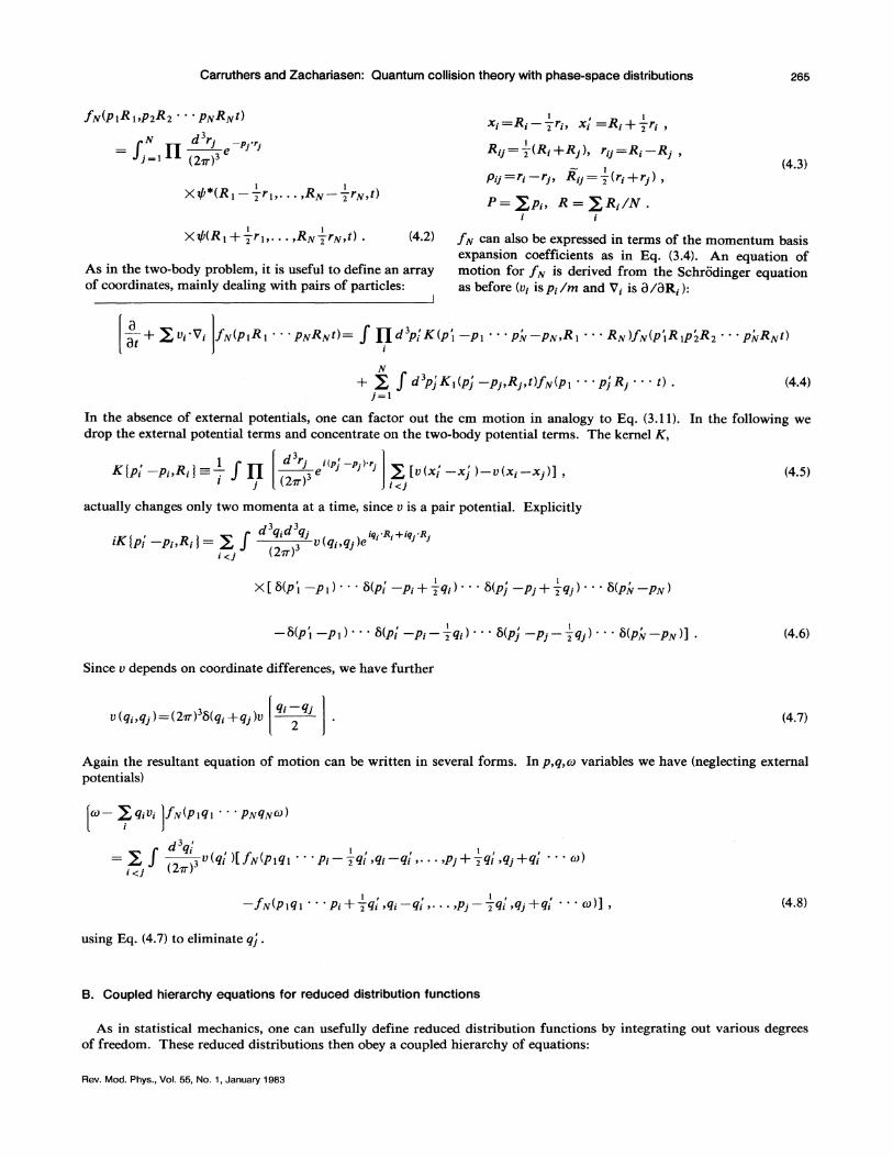
Carruthers and Zachariasen: Quantum collision theory with phase-space distributions 265
R I , I X;= ;--zr;, X; =R;+-zr;,
I Rii=-z(R;+R1), rij=R;-Ri,
- I Pii =r; -r1, Rij = -z(r; +r1 ) ,
(4.3)
P= ~p;, R = ~R;/N. ; i
As in the two-body problem, it is useful to define an array of coordinates, mainly dealing with pairs of particles:
f N can also be expressed in terms of the momentum basis expansion coefficients as in Eq. (3.4). An equation of motion for f N is derived from the Schrodinger equation as before (v; is P; lm and V; is a;aR; ):
[ :t + ~v;·V; ]tN(p,R, · · · PNRNt)= J I;Id 3p[K(p',-p, · · · PN-PN,Rl · · · RN)fN(p'1R 1p'zR 2 • • • PNRNt)
N
+ ~ f d 3pj K, (pj -pi,RJ,t)fN(Pl · · · pj Ri · · · t) . (4.4) j=l
In the absence of external potentials, one can factor out the em motion in analogy to Eq. (3.11). drop the external potential terms and concentrate on the two-body potential terms. The kernel K,
, 1 J II [ d 3rj i(p~ -p.)·r·] ~ , , K{p· -p· R·J =- --e 1 1 1 [v(x· -X· )-v(x·-X·)] I I' I • , ( 2 )3 , , I J I J >
l J 1T' 1 <)
actually changes only two momenta at a time, since v is a pair potential. Explicitly
f d 3q;d 3qj iq.·R·+iq.·R· iK{p[-p;,R;)=~ (21T')3 v(q;,q1)e 1 1 1 '
i<i
Since v depends on coordinate differences, we have further
In the following we
(4.5)
(4.6)
(4.7)
Again the resultant equation of motion can be written in several forms. In p,q,w variables we have (neglecting external potentials)
(4.8)
using Eq. (4.7) to eliminate qj.
B. Coupled hierarchy equations for reduced distribution functions
As in statistical mechanics, one can usefully define reduced distribution functions by integrating out various degrees of freedom. These reduced distributions then obey a coupled hierarchy of equations:
Rev. Mod. Phys., Vol. 55, No.1, January 1983

266 Carruthers and Zachariasen: Quantum collision theory with phase-space distributions
N
J';J><ptRtt>= I II d 3pjd3RjfN<PtR! ... PNRNt)' i=2
N
JJ1><ptR!p2R2t>= I II d 3pjd3RjfN<PtR! ... PNRNt)' i=3
N Jiv">(p!Rl ... p,R,t)= I II d 3pjd3RjfN<PtR! ... PNRNt).
i=n+l
Note that inp,q,w language the space integrations amount to setting q =0, N
JJJ'><ptqt ... p,q,w)= I II d 3pJfN<Ptqt · · · p,q,.pn+tO · · · PNO,w). j=n+l
Applying this rule to the equation of motion to get J}J >, we find
d3q~ (w-q_t"!Lt )jjJ>(plqtw>= 1: I d 3p2 · · · d 3pN-( ')3 v(qj)
l<i 2~
(4.9)
(4.10)
Note that q1 is always zero, since j > i ~ + 1. Now consider separately the i = 1 and i > 1 terms on the right-hand side. For i = 1 we find
d3 , 1: I ~v(qj) I d 3p2 · · · d 3pN[JN<Pt-Tq't.qt-q!p20, ... ,pi+Tq't.q! , ... ,pNOw) J> I (2~)
recalling the definition of /(2). This equation has N -1 equal contributions to the sum. All terms having i ~ 2 cancel, as shown by the following expression:
d3 , ~ I (2 q)23 I v(qi ld 3P2 • • • d 3PN[fN<Ptqt>P2- Tqi, -qi,. · · •Pi +Tqi,qi,. · · ,pNOw) J>2 ~
(4.12)
(4.13)
Now the apparent ±qi /2 dependence of the p 2 and p1 arguments can be removed by shifting integration variables and canceling. We are left with
d3 , (w-qt"!Lt >JiJ><ptqtw)=(N -1) I ~v(q't) I d 3p2[JJI><Pt- Tq't ,qt -q't ,p2 + Tq'tq't.w)
- (2~)
(4.14)
For N =2 this reduces to the equation formed before [Eq. (3.27)] in the two-body problem. Note that, if desired, we may remove the q] variable accompanying the p 2 integration.
For N =2 we encounter a new feature which extends to all higher-order distribution functions. Proceeding as before, we find
(w-qt"Vt -q2 ·v2 >JJ1><ptqtp2q2w)
d3 , =~.I (2 q)13 v(q't) I d 3P3 · · · d 3pN[JN(Ptqtp2q2P30,. · · ,p;-+q; ,q;-qi ,. · · ,pi+Tqi ,qi+q/ ,. · · ,pNOw)
I<J ~
-fN(Ptqtp2q2P30,. · · ,p;+Tqf ,q;-qj ,. · · ,pi-Tqf ,qi+q/ ,. · · ,pNOw)] ·
(4.15)
Rev. Mod. Phys., Vol. 55, No.1, January 1983
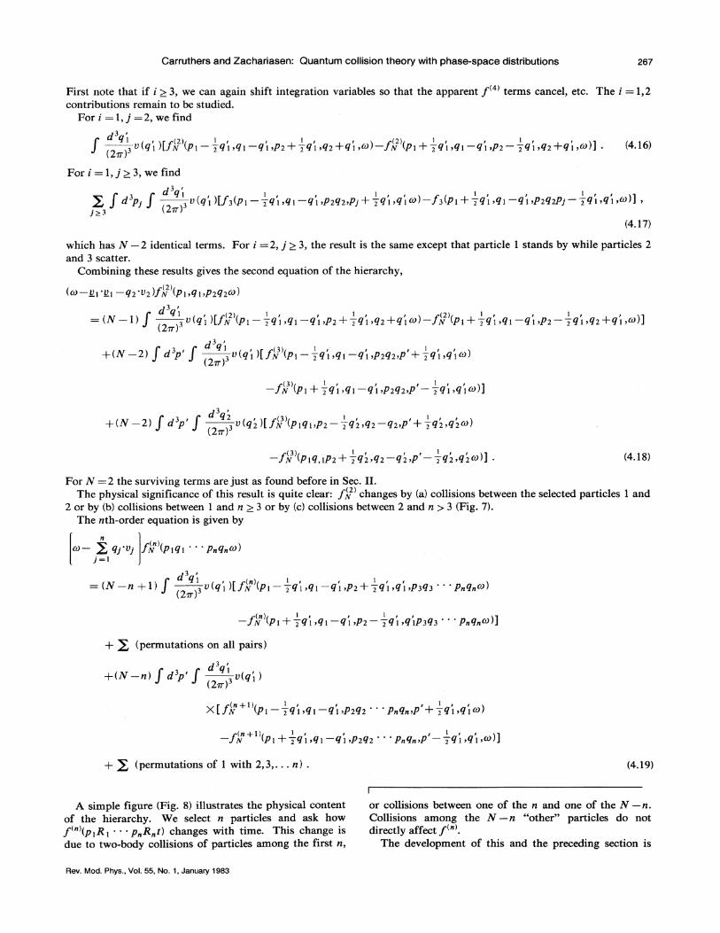
Carruthers and Zachariasen: Quantum collision theory with phase-space distributions 267
First note that if i ~ 3, we can again shift integration variables so that the apparent /<4> terms cancel, etc. The i = 1,2 contributions remain to be studied.
Fori= 1, j =2, we find
d3 ' f q I ( , )[/(2)( I , , I , , ) /(2)( I , , I , , )] (21T)3 v ql N P1-2q1 ,ql-qt ,p2+2q1 ,q2 +q1 ,w - N P1 +-zql ,ql -ql ,p2 --zql ,q2+q1 ,w . (4.16)
which has N -2 identical terms. For i = 2, j ~ 3, the result is the same except that particle 1 stands by while particles 2 and 3 scatter.
Combining these results gives the second equation of the hierarchy,
(w-QI'1LI-q2·v2>fJJ>(p"q"p2q2w)
d3 ' (N 1) f q I ( , )[/(2)( I , , I , , ) /(2)( 1 , , 1 , , )]
= - (21T)3 v ql N P1-2q1 ,ql -ql •P2 +-zql ,q2+q1w - N P1 +-zql ,ql -ql ,p2-2q1 ,q2 +q1 ,w
d3 ' (N 2) f d 3 • f ql ( • )[/(3)( I , , 1 1 , , ) + - P (21T)3 v ql N P1 --zql ,ql-ql>pzqz,p +-zql ,qlw
(4.18)
For N =2 the surviving terms are just as found before in Sec. II. The physical significance of this result is quite clear: JJJ> changes by (a) collisions between the selected particles 1 and
2 or by (b) collisions between 1 and n ~ 3 or by (c) collisions between 2 and n > 3 (Fig. 7). The nth-order equation is given by
[w- ~ qj'Vj ]Jj.;>(plql · · · Pnqnw) ]=I
+ ,l: (permutations on all pairs)
d3q• +<N -n) J d3p' J __ 13 v(ql)
(21T)
+ ,l: (permutations of 1 with 2,3, ... n) .
A simple figure (Fig. 8) illustrates the physical content of the hierarchy. We select n particles and ask how J<n>(p 1R 1 · · · PnRnt) changes with time. This change is due to two-body collisions of particles among the first n,
Rev. Mod. Phys., Vol. 55, No.1, January 1983
(4.19)
or collisions between one of then and one of theN -n. Collisions among the N - n "other" particles do not directly affect J<n>.
The development of this and the preceding section is

268 Carruthers and Zachariasen: Quantum collision theory with phase-space distributions
H H H 2 3 2 3 3 2
FIG. 7. Three kinds of contributions to the equation of motion for f 2 [see Eq. (4.18)]. In (a) the two chosen particles scatter, while in (b) and (c) one of the chosen particles scatters off a particle in the medium while the other chosen particle is unaffected.
completely general insofar as it is only a restatement of the N-body equations of motion in phase-space language. However, as soon as we postulate boundary conditions or make an approximation to the hierarchy (typically factorization, leading to truncation), careful attention has to be given to physical requirements. For example, in a collision of composite systems, the particles in a bound state are always correlated initially, and one cannot factorize a distribution function in the variables of the bound state.
In the scattering of composites having N 1 ,N 2 particles (Ni assumed large), there can be a region of space-time in which the dynamics can be described by kinetic equations of the traditional type. As a preliminary to the discussion of scattering of composites, we review in our formalism some traditional simplifications possible for large (not necessarily uniform) systems.
Assuming that particles 1 and 2 are uncorrelated, i.e.,
f( 2 )(p 1R 1,p2R 2t)=J0 >(p 1R 1tl/( 1>(p2R 2t) ,
we obtain a nonlinear equation for/(!)'
This is the usual mean-field theory expressed in phasespace language, where the effective potential energy of a particle is
Verr(q! ,t)= V(ql ,t)
+(N -l)v (ql) J d 3pzf0 >(pz,ql ,t) .
(4.23)
Equation (4.22) is the time-dependent Hartree-Vlasov equation in which the distribution /( 1 > may be imagined to be found self-consistently. When linearized, it gives a random-phase approximation which exhibits under suitable circumstances collective modes such as plasmons and
Rev. Mod. Phys., Vol. 55, No.1, January 1983
H n N-n n N-n
FIG. 8. Contributions to the n-particle reduced distribution function. These comprise a simple generalization of Fig. 7.
C. Truncation schemes and the Boltzmann-VIasov equation
Although there is no way to legitimately avoid the Nbody problem, many physical quantities depend on highly averaged objects like the one- and the two-body distribution functions. In many cases, physically motivated (but mathematically dubious) approximations, such as truncation, neglect of correlations, etc., lead to good results with highly intuitive content. In traditional subjects these approximations are associated with the names of Hartree, Vlasov, and Boltzmann. The validity of these approximation schemes in complicated scattering and reaction processes remains to be studied. As a preliminary, we show how the Vlasov and Boltzmann equations can be extracted from our formalism.
The equation of motion for the one-particle distribution functions including a time-dependent external potential is
(4.20)
(4.21)
(4.22)
zero sound in uniform systems. For a system of electrons (neutralized by a constant
positive background) the resultant equation is the Vlasov equation. We review the case of small oscillations about a spatially uniform Maxwellian distribution normalized to one particle per unit volume:
fo(p,R,t) exp( -p 2 /2mkT)
(21TmkT) 312
(4.24)
(4.25)
If we assume f' to be of order V(qltl, linearization gives

Carruthers and Zachariasen: Quantum collision theory with phase-space distributions 269
j'(p,q,(J)) =X (p,q,(J))
X [v<q,(J))+(N -Ov(q) f d 3p'j'(p',q,(J))],
(4.26)
fo(P -+q>-fo<P ++q> X(p,q,(J)) = ----.----
(J)+IE-_q'.!lp
The solution is
/'(p,q,(J))= V(q,(J))Xfp,q;(J)> . (4.27) 1-(N -l)v(q) d pX(p,q,(J))
If collective modes exist for frequency (J)(q), then f' can be finite for arbitrarily small V(q,(J) ). The eigenvalue equation is
f (p- ..!..q>-I (p + ..!..q> l=(N -l)v(q)P f d 3p 0 2 0 2 ,
(J) - _q 'll.p
(4.28)
where P stands for the principle value. In the Coulomb gas, we can find the plasmon root for q-->-0 by expanding the integrand,
l=(N -l}v(q) J d 3p [ -_q·Vp/0 (p)
X [ ! + q ·~~m + . . . ) ] '
(4.29)
2 4TrNe 2 (J)pl = ---v;;;- .
A more detailed discussion is given by Brout and Carruthers (1968). Here we have converted N to a density N IV to conform to our normalization.
All these results are well known. To proceed, we want to place the above in a more ambitious context, that of improving the above ·approximation to obtain the Boltzmann collision terms. Suppose we integrate formally the equation for t<2l to include collisions between 1 and 2, but ignore correlations in fm. This approximation leads to the usual Boltzmann equation with the cross section evaluated in lowest Born approximation, but with a particular factorization approximation for t< 3>.
For our approximate/< 2 >, we make the ansatz
(4.30)
f 1 is then the solution to Eq. (4.20) with f2 ->-f2 • Formally this is the two-body scattering problem in the absence of the rest of the system, without, however, the em momentum constraint, i.e., p 1 +p2 is not some fixed constant. To see in what sense this is an approximate solution, we apply D /Dt to this expression using the equation of motion [Eq. (4.20)] for fn,
. a -(2) q I , P{2) I , , I , [ ] dJ I
'at-q,·v,-q2'V2 f = J (21T')3v(q,)[/ (p,-Tql,ql-qt,P2+Tql,qlt)
(4.31)
Comparing with the exact equation of motion for t<2l, we see that the approximation t<2l = J<2l corresponds to the following factorization:
(4.32)
etc., i.e., factorization of the one-particle distribution for the unscattered particle, and secondly N -1 ~N -2, requiring N >> 1 for validity.
Rev. Mod. Phys., Vol. 55, No.1, January 1983

270 Carruthers and Zachariasen: Quantum collision theory with phase-space distributions
Clearly, a similar procedure can be adopted in any order: factor then+ 1-particle distribution suitably and solve for f(n) each n in turn. "Suitable" factorization is a subject for further study, and the question of convergence is completely open.
For the moment, our ambition is only to show how both the Boltzmann and the Vlasov contributions to the oneparticle transport equation follow systematically from our ansatz for f 2 l. Iterating once by substituting /(2) into the right-hand side of Eq. (4.20), we find
[ a ] I.!f.!L_ I I i-a -qv ! 0 )<p,q,t)- 3 Veff(q',t)[f0 )<p-2q',q-q',t)-f0 )<P+2q',q-q',t)] t (21T)
X[/(2)(p --fq'--fq",q -q'-q",p'+-fq'
+ -fq",q' +q",t')- f(2)(p--fq' + -fq",q -q'-q",p'
+ -fq'- -fq",q' +q",t')]
t [ [ p+.}_q' p'-.}_q'] ] +I_ 00 dt'exp -i (q-q') m2 +q' m2 (t-t')
x[f2)(p +-fq'--fq",q -q'-q",p'--fq'
+ -fq",q' +q",t')- f(2)(p + -fq' + -fq",q -q'-q",p'
I I } -2q'-2q",q'+q",t')] , (4.33)
where Verr (a functional of / 0 )) is defined in Eq. (4.23). The expression involving Verr is easily identified with the "force" term - VV(/i,t)·V pf0 )(P,R,t) appearing in the
usual Boltzmann equation. To see this, expand 1< 1 l(p 1 ± -fq 1 ) about p 1, getting
dJ I . I ~[ -q'V err(q',t)]·Vp/(l)<e,q -q',t)= -i I d 3R e -I!·K[VVerr<R,t)·Vp/0 l(p,R,t)] , (4.34) (21T)
where in this case V err is given by the second term of Eq. (4.23). Thus in pRt variables the left-hand side has the familiar form
i [ :t +v·VR- VVerr·VP k(l)(J!.,R,t) . (4.35)
In order to manipulate the right-hand side of Eq. (4.33) to recognizable form, we work in w space, where the time exponentials appear as energy denominators. We obtain
(N-l)I d 3q' J!DL.Id 3p'v(q')v(q")(l+l) (21T)3 (21T)3 I 2 '
1 J1= I I
(p-2q') (p+2q') w-(q -q')· -q'·----
m m
X[/( 2)(p --fq'--fq",q -q'-q",p' +-fq'+ -fq",q' +q",w)
- f2l(p- -fq' + -fq",q -q'-q",p' + -fq'- -fq",q' +q",w)] , (4.36)
Rev. Mod. Phys., Vol. 55, No. 1, January 1983

Carruthers and Zachariasen: Quantum collision theory with phase-space distributions
1 1z= •
(p+2q') w-(q -q')·---=-
m
(p'-+q') q'·--....;;_
m
X[/< 2l(p ++q' -+q",q -q' -q",p' -+q' + +q",q'+q",w)
-/<2l(p + +q' ++q",q -q' -q",p' -+q•-+q",q' +q",w)] .
271
At this state, it is not necessary to factorize /(2). However, it will be very helpful to first study the spatially homogeneous case in which
t< Jl(p,q,ru)=(21dl>(q)/0 l(p,ru) ,
f< 2l(plqlpzqzw) =(21dl>(ql )l)(q2 )/<2l(PIP2ru) · (4.37)
The integrand contains the common factor l>(q' +q")l)(q). term here)
Canceling and simplifying leads to (dropping the Vlasov
ru/0 l(p,ru)=(N -1) J d 3q'3 I v(q') 1 2 J d 3p'(lj +12), (21T)
1 1j =----___;:..___--,2--[f(2)(p,p',ru)-/<2l(p -q',p +q',w)], w+q'· (p -p') !L:_+i£
m m
1i = -----1:::.._-~--[f(Z)(p +q',p -q',w)-t<2l(p,p',ru)] . (p -p') !L!._
w+q'· . + +i£ m m
We now combine terms by setting q'--+ -q' in 12. Noting the identity
- - q'·(p -p') !i:_ AE =Ep + Ep·-EP -q'-Ep· +q'- ..&---"--___.--'--
m m
we find
(4.38)
(4.39)
ru/0 l(p,ru)=(N -1) J ~I v(q') 12 J d 3p' . - . [J<2l(p,p',ru)-f 2l(p -q',p' +q',w)]. d3 I [ 1 1 ] (21T)3 A.E +w+l£ AE -W-l£
(4.40)
The energy difference in [Eq. (4.39)] has a clear pictorial significance in scattering theory. For a givenp;p',q', this I::.E defines a collision time Tcon-li/ I::.E. If Tcoll is much less than the characteristic time in which f changes, then for significant portions of the integrand w << AE and the energy denominators produce an energy-conserving delta function -21Til>(AE) of just the right character to yield the cross section necessary for the Boltzmann equation.
To make this argument more precise, we transform back from w to t, getting
Cl/(p,t) = -(N -1) J _!f!L_ I v(q') 12 J dlp• J' dt'ei<I!.El<t-t'l+e-l<b.E)(t.-t'l at (21T)3 -"'
x[J<2l(p,p',t')-J<2l(p -q',p'+q',t')]. (4.41)
Since AE -1/7", iff varies slowly on a time scale compared with -r, regions of the integrand with t -t' >>T contribute. So we evaluate f 2l at t' ~ t and do the time integrals directly. In this limit only t' ~ t matters: the system has lost its memory and becomes stochastic. The effective time integral is now J _"'.., eii!.E-rd-r, giving
ilf~~,t) (N -1) J d 3p' J (~~)~ I v(q') I221Tl>(/::.E)[fm(p -q',t)f0 l(p' +q',t)-J 0 l(p,t)/0 l(p',t)] . (4.42)
which is the usual form of the homogeneous Boltzmann equation, on identifying
(4.43)
Rev. Mod. Phys., Vol. 55, No.1, January 1983
as the transition rate for p +p'--+(p -q')+(p'-q'). For bosons or fermions, obvious corrections need to be made to the occupation probabilities.
Intuitively, one expects that for a dilute gas the scatterings occur on-shell, and that in the above one can substi-

272 Carruthers and Zachariasen: Quantum collision theory with phase-space distributions
tute v---+t, where t describes the scattering to all orders in v. This supposition is encouraged by the fact that jl2 >
obeys the full two-body scattering equation. For dense systems, one can expect significant energy shifts, off-shell, and lifetime effects. This aspect of the problem has been analyzed by Snider ( 1960) and others.
The classical collision time for a potential of finite range a is given by VTcJ""='a, where v is the relative velocity:
- 1 :::;::::KIP-P 1 11m. Tel
(4.44)
K = 1 I a is the maximum momentum supplied by the potential. In contrast the quantum collision time determined by Eq. (4.39) is not given by K although since I q 1 I <K there is a bound
1 K lp -p 1 I K 2 -< +-. (4.45) Teall- m m
For that set of collisions having I p - p 1 I > K the upper bound of Eq. (4.45) coincides with Tci·
The relaxation time T provides a key to the question of energy conservation. From Eq. (4.42) we can define arelaxation time, describing the scattering out of momentum states p,p 1 :
1 1 a1 N -=---=-va T 1 at v (4.46)
for large N, with V the volume and u the usual cross section. Equation (4.46) is equivalent to the traditional
Our ansatz for 12 corresponding to Eq. (4.30) is
f2(pjR tPiR2t)= It (pjRttllt (pi_R2t)
mean-free-path formula, I =(pu)-1 with p=N IV the number density. From Eq. (4.46) we see that
I :E I""" T~n ' (4.47)
confirming the argument given after Eq. (4.40). Comparing Eq. (4.44) with Eq. (4.46) gives
For a dilute gas, a II is very small. Several dimensional parameters play a role when we
consider systems of finite size: for example, in a nucleus we have the interparticle distance and the surface thickness as well as the potential size as length parameters.
Baym and Kadanoff ( 1962) have discussed the form of the Boltzmann equation in the case of a slowly varying external potential. Under suitable circumstances, the net result is to consider Eq. (4.42) locally valid, i.e., each l(p,t) is replaced by l(p,R,t) with a common R. For applications to scattering problems as contemplated here, the inhomogeneities are much greater, so that genuine retardation effects must be retained. We now repeat in coordinate space a sequence of approximations similar to that leading to the spatial uniform Boltzmann equation (4.42). We leave in abeyance the question of the relative validity of the factorization approximation in the two cases.
The coordinate-space version of Eq. (4.14) is
-i J~,., dt 1 J d3p"d3p" "( "- )• I "( " I )• I-1 2 I P1 P1 '1 I P2 -pi '21 ( "Rret "Rret 1)
(21T) 3 e e 2 P t t P2 2 t
[ (R ret I 1 R ret I , ) (R ret I , R ret I , )] X v t +-zrt- 2 --zr2 -v t --zrt- 2 +-zr2 , (4.50)
with Rr=R;-p[ (t -t1 )lm. Substituting this in Eq. (4.49), relabeling, and dropping the Vlasov term for simplicity, we obtain a generalization of
Eq. (4.38),
alt(p,R,tl at +v·VIt(p,R,t)
d3q d3q =-(N-OJ 1 2d3Rid3 I
(21T)3 p
Jt i(q 1+q2 )(R-R') [ • [p-p 1 +T(q1-q2)](t-t1)
X dt 1e v(q 1 )v(q2 )exp -lq2-----------_,., m
[ - [ ~ P+Tq!(t-tl) I I P1 +Tq2(t-t1 ),t' X l2 P+ 2 (qt+q2),R- ,p,R --------
m m
Rev. Mod. Phys., Vol. 55, No. 1, January 1983

Carruthers and Zachariasen: Quantum collision theory with phase-space distributions 273
[ [p-p'-~(ql-q2)]] xexp -iq2 ~ (t -t')
This result is only the spatial analog of Eq. (4.36), but is more amenable to approximations based on space-time intuition. For example, we can study the conditions under which Boltzmann's equation applies locally.
First note that when the distribution functions are uniform in the space coordinates, the retardation factors in the arguments of f 2 drop out, leaving a time integral which reproduces the energy denominators of Eq. (4.38). The reader can confirm by a straightforward calculation that Eq. (4.51) reduces to Eq. (4.38) in this limit. Note, in particular, that the R independence of 12 yields ~(q 1 +q2), a necessary ingredient in producing the collision cross-section factor. As before, when f varies slowly on the scale of a collision time, one gets the on-shell energy-conserving delta function.
Again, for slowly changing j(t), the t' integration is restricted to a range at =t -t' :;::,alv where a is the potential range [cf. Eq. (4.44)]. In that case, the retardation terms are negligible, i.e., R ±a ,.,R, provided f changes slowly over the distance a. Now consideration of the exponential (q 1 +q2 HR -R') shows that R' cannot differ by more than a from R, allowing us to write R'~R in / 2 •
Finally, we obtain again l>(q1 +q2) from the R integration, which gives us the local version of Eq. (4.42) upon factorization.
At the surface of a nucleus, the retardation distance is of the same order as the surface thickness, and the local approximation will be wrong. Within the nucleus, the situation is better, insofar as aiR ,.,o. 7al A 113 (a in fermis). For a~ 1.4/, A =216, we have aiR ::::,0.12, but for A =27, aiR :;:::,0.33, not negligible. Further, when bound-state effects are included (with oscillating phasespace densities), it is not clear whether the whole approach makes sense. Further research will be required to clarify this situation for realistic problems.
D. Hydrodynamic equations
As in the case of the one-particle potential problem, hydrodynamic equations follow immediately on taking suit-
Rev. Mod. Phys., Vol. 55, No.1, January 1983
(4.51)
able moments of the equations of motion. It is significant to note that these formal structures are quite independent of boundary conditions or assumptions regarding local thermodynamic equilibrium. The deduction of hydrodynamic and transport equations has an extensive history, which is reviewed by Mori, Oppenheim, and Ross ( 1962) and de Groot and Suttorp (1972).
From the particle density
p(R)= ~~(B. -B.;)'
we construct the averaged density
n (B.,t)= II J d 3p;d 3R; i
(4.52)
X ~l>(B.-B.a>fN(PtRt · · · PNRNt) · a
(4.53)
This definition, which treats all particles symmetrically, differs by a normalization factor N from Eq. (4.9).
Imitating the calculations of Sec. II.G leads directly to the continuity equation [Eq. (128)], with
n (£,t)H(B.,t>= II J d 3p;d 3R; i
(4.54)
Multiplying the equation of motion with the average velocity
~ P; ~(R-R·) ; m '
(4.55)
and integrating over phase space gives the momentum equation analogous to Eq. (2.131):

274 Carruthers and Zachariasen: Quantum collision theory with phase-space distributions
(4.56)
Manipulation of the drift term leads to the analog of Eq. (2.136),
i aa. f rr d 3pkd 3Rk 1: v~v!t><R -Ra)f(plR I ... PNRNt)=i aRa [n (R,t)( u'uk) 1 . ~ a I
(4.57)
On the right-hand side the potential terms act as forces-one due to the external fields V and the other due to all the particles other than the chosen one at point ,R.
Explicitly we have for the right-hand side of Eq. (4.56):
i f 3 3 [ av av<Ra-Rp)] .n(R,t) -- _l: fi d Pkd Rkl>(R -Ra) aR (Ral+ _l: aR j(p1R1 · · · PNRNt)==. -z--[VVex+VVind. m a a ~a p m
The equation of motion for the momentum density is then very similar to that for the one-particle result [Eq. (2.131)]:
a a ) n at(nu;)+ aR. (n(U,Ui )=--;;<VVex+VVintl. I
(4.59)
As before [Eq. (2.137)], one can manipulate Eq. (4.59) into the form of Euler's equation.
The existence of these formal structures in no way assumes local equilibrium or classical approximations. Naturally, the calculation of the quantities appearing in the equation requires a knowledge of the distribution functions, i.e., a solution of the N-body problem.
E. Formulation in second quantization
The correct description of the many-body system requires that close attention be paid to the particle statistics and the spin and internal symmetry (e.g., isospin) variables of the problem. The preceding development has ignored these cumbersome technical details in order to express more clearly the structural aspects of the theory. Although the structure of the N-body wave function has been much studied with regard to these questions, it is often expeditious to use the compact notation made possible by the formalism of "second quantization." The equivalence of this approach to the usual N-body Schrodinger equation is explained in textbooks by Huang (1963), Schweber (1961), and Fetter and Walecka (1971).
The dynamical coordinates in the Heisenberg picture [(.,P(;I,t) and its adjoint .,p+(;I,t)] obey the commutation or anticommutation rules,
[ tfa(,!.,t,.,P$"(,!.',t )J± =l>apl>(,!. -,!.') '
[.,P(;I,t},.,P(;I',t}]±=O,
Rev. Mod. Phys., Vol. 55, No. 1, January 1983
(4.60)
(4.58)
for boson or fermion fields. Here a and {3 denote labels for any discrete internal variables such as spin and isospin.
The generalized (matrix) Wigner function is then defined in terms of the density operator p by
f ap(f!_,,R,t)
-J d 3t -i.P':! + I I = (21de - Tr[p¢a<R-T.r.,t).,Pp(E.+T.t,t}].
(4.61)
For a pure state involving the wave function I .,P), we have p= I 'II) ('II I . In particular, for a one-particle state this is completely equivalent to the definition (2.92} (except the order of indices, which is a matter of convention).
The total number density is now
,l: J d 3pfaa(f!_,,R,t)=Trp¢+(E_,t}.,P(,R,t) a
(4.62)
If we expand .,P in the momentum basis as in Eq. (2.2), with C(f!_,t )_,.aaV!_,t} being destruction operators obeying
[aa(f!_,t),a$ (f!_',t)]± =l>apl>(f!_ -f!_') ,
[aa(f!_,t),ap(f!_',t)J±=O,
we find the alternative form
(4.63)
f d 3q -iq·B, [ + ( I ) ( I ] lap= --3 e - Trpaa P+Tq,tapp-Tq,t). (21T)
(4.64}
The pair operator a/+qap is useful in describing density fluctuations and plays a prominent role in the many-body problem.
Integrating over phase space gives (dr==.d 3p d 3R}
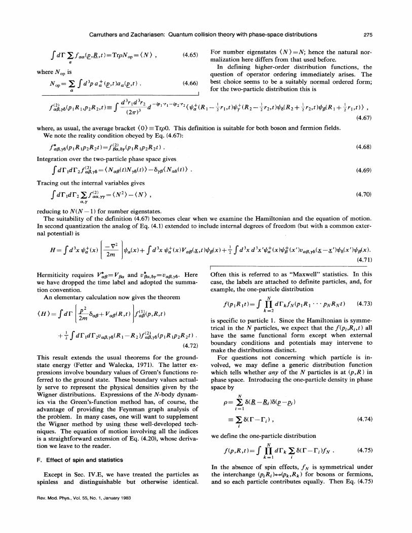
Carruthers and Zachariasen: Quantum collision theory with phase-space distributions 275
I dr ~~ aa(p_,B_,t)=TrpNop= (N) , a
whereN0 p is
N 0 p= ~I d 3pa"/;(p_,t)aa(p_,t). a
(4.65)
(4.66)
For number eigenstates ( N) =N; hence the natural normalization here differs from that used before.
In defining higher-order distribution functions, the question of operator ordering immediately arises. The best choice seems to be a suitably normal ordered form; for the two-particle distribution this is
where, as usual, the average bracket ( 0) = TrpO. This definition is suitable for both boson and fermion fields. We note the reality condition obeyed by Eq. (4.67):
J:p,rtJ(piR iP2R2t)=fi).,llr(PiR 1P2R2t) ·
Integration over the two-particle phase space gives
I drldr2f~1-J.y8= (N afJ(t)N y8(t)) -Byp(N all(t)) .
Tracing out the internal variables gives
I ariar2~f~1.j..rr= (N2)- (N) , a,y
reducing to N(N -1) for number eigenstates.
(4.68)
(4.69)
(4.70)
The suitability of the definition (4.67) becomes clear when we examine the Hamiltonian and the equation of motion. In second quantization the analog of Eq. (4.1) extended to include internal degrees of freedom (but with a common external potential) is
H =I d 3x t{J"/;(x) [ ~;2 ]t/Ja(x)+ I d 3x t{J"/;(xlVap(~,t)t{Jp(xl+-i- I d 3x d3x't{J"/;(x)t{J"j(x')va{J,yll(~ -~')t/Jil(x')t{Jp(x). (4.71)
Hermiticity requires V:p= V fJa and vP<z,llr=VafJ,rtJ· Here we have dropped the time label and adopted the summation convention.
An elementary calculation now gives the theorem
(H)= I dr [ f~ Bap+ Vap(R ,t) k~~(p,R,t)
This result extends the usual theorems for the groundstate energy (Fetter and Walecka, 1971). The latter expressions involve boundary values of Green's functions referred to the ground state. These boundary values actually serve to represent the physical densities given by the Wigner distributions. Expressions of the N-body dynamics via the Green's-function method has, of course, the advantage of providing the Feynman graph analysis of the problem. In many cases, one will want to supplement the Wigner method by using these well-developed techniques. The equation of motion involving all the indices is a straightforward extension of Eq. (4.20), whose derivation we leave to the reader.
F. Effect of spin and statistics
Except in Sec. IV .E, we have treated the particles as spinless and distinguishable but otherwise identical.
Rev. Mod. Phys., Vol. 55, No. 1, January 1983
Often this is referred to as "Maxwell" statistics. In this case, the labels are attached to definite particles, and, for example, the one-particle distribution
N j(piRit)= I n drkfN(PiRi ... PNRNt) (4.73)
k=2
is specific to particle 1. Since the Hamiltonian is symmetrical in theN particles, we expect that the j(pi,Ri,t) all have the same functional form except when external boundary conditions and potentials may intervene to make the distributions distinct.
For questions not concerning which partiCle is involved, we may define a generic distribution function which tells whether any of theN particles is at (p,R) in phase space. Introducing the one-particle density in phase space by
N p= ~ B(B_-B.;)B(p-pi)
t=i - -
we define the one-particle distribution N
j(p,R,t)= I nark ~B(r-ri)/N. k=i i
(4.74)
(4.75)
In the absence of spin effects, f N is symmetrical under the interchange (piRi )++(pk,Rk) for bosons or fermions, and so each particle contributes equally. Then Eq. (4.75)
276 Carruthers and Zachariasen: Quantum collision theory with phase-space distributions
differs only by a normalization factor N from Eq. (4.73), as in the Maxwell case.
Of course, the true wave function typically contains spin variables (and perhaps others) in addition to the space coordinates. Then f must be labeled suitably to handle the spin coordinates. Ordinarily, the wave function will be decomposed into irreducible representations of the permutation group in the form of products of spin and space functions of possibly rather complicated mixed symmetries. In some cases, the spin complications may be significant, each problem being treated on its own merits.
The simplest example is a two-particle fermion system composed of one-particle states,
(4.76)
where the labels i and j indicate the one-particle-state quantum numbers. We take i=j=j, since otherwise tf; vanishes. For simplicity, let u; be energy eigenstates carrying spin +. The two-particle distribution function is
fii(piRipzRz)=fu(PIRI )fiJ(pzRz)
+ /;;(pzRz )filPIR 1)
-f11 (p 1R 1 )/11 (pzRz)
-/;i(pzRz)/i;(piRI).
Integration according to the rule (4.75) gives
j(p,R) = f 11 (p,R )+ J11 (p,R) .
(4.77)
(4.78)
We can, of course, decompose the wave functions according to spin 0 and spin 1, i.e., symmetric or antisymmetric space states,
'l'o= ~ [q:>a(XI )q:>b(xz)+q:>b(xl lq:>a(Xz)]XS=O,
(4.79) I 1 S=l
'I'M= V2 [(f'aa(xl)(/ib(Xz)-q:>b(xl)q:>a(Xz)]XM •
In analogy to the one-particle case (2.125), Wigner function in the coupled spin basis
SS' I + f M. M.' - \II S' M.' \II SM. •
we write a
(4.80)
Tracing on the spin components gives Bss· and independent Wigner functions for each spin. Of course, the potential may couple the fs in such a way as to require the full matrix set (4.80). The basis (4.80) [more general than the example wave function of (4.79)] is generally the most useful in practical problems.
Next consider the one-particle distribution for a Slater determinant of one-particle functions (Moya1, 1949; de Groot and Suttorp, 1972):
1 'II= 112 l: ( -OPPu1(llul2l · · · up(N), (4.81)
(N!) P
where the subscripts label the occupied single-particle states (all distinct by the antisymmetrization). Integration
Rev. Mod. Phys., Vol. 55, No.1, January 1983
according to Eq. (4.75) immediately leads to
j(p,R,t)= l:J11(p,R,t), I
(4.82)
where/;; is the one-particle Wigner function for state i. Equation (4.82) corresponds to representing theN-particle density matrix as the sum of one-particle density matrices.
The one- and two-particle distributions for Maxwell, Bose, and Fermi product wave functions are given in Chap. VII of de Groot and Suttorp (1972).
A semiclassical evaluation of the Wigner function for a one-dimensional Fermi gas in a potential well has been given by Balazs and Zipfel (1973). Shell-model calculations involving a "smeared" Wigner function have been presented by Baker, McCarthy, and Porter (1960). Comparison with the Thomas-Fermi model has been made in both these works.
V. POSSIBLE APPLICATIONS IN INTERACTIONS OF COMPOSITE SYSTEMS
A. Composite particle scattering in the Liouville formalism
The enormous variety of possible final-state channels, and the complexity of the time evolution leading to those final states, require a cumbersome formal apparatus reviewed by Goldberger and Watson (1964) and Newton (1966) for the usual Hamiltonian formalism. The additional complications caused by particle identity and statistics will be generally ignored in our outline. A cartoon of the physical situation is given in Fig. 9. We envision the collision of two bound systems having N 1, N 2 particles. Figure (9b), suitable for short-range forces, indicates interaction in the overlapping region. Following an extensive interaction in the collision volume [Fig. 9(c)], the system separates into final states comprising all imaginable bound-state configurations [Fig. 9(d)]. In describing these final states, it is traditional to speak of "channels" and "channel Hamiltonians" in which interactions between constituents in distinct bound states are ignored. A given channel involves a partition of the total number of final bound particles N =N;% N a + · · · +N a , with the
I 2 k
individual final particles labeled by a1• Each of these partitions corresponds to an asymptotic wave function <l>a, with the total wave function given by
(5.1)
There is some model dependence tacit, in that an excited state with lifetimes greater than the transit time to the detector will count as a "bound state."
We should also note the expression of translation invariance, which allows one to factor out the overall em motion in direct extension of the two-body problem, as in Eq. (3.11)ff. Introducing total and relative coordinates by

Carruthers and Zachariasen: Quantum collision theory with phase-space distributions 277
Xtz=Xt-Xz •
(5.2)
and factoring out the em motion as
'II =X(X,t )~(XIj•t) (5.3)
leads to the expression for the Wigner function:
fN(PtRI · · · PNRNt)=foU!.,Ji,t)fN(Pii•Rii•t), (5.4)
where the variables are N
P=~P1 , i=l
N
R = ~ R 1/N, r= ~r;IN, 1=1
C?--8 Nz
co •
'o 1 c/ ..----.... • ~
/ \
(S.5l
(a)
(b)
(c)
(d)
FIG. 9. Simplified version of the stages of a nucleus-nucleus collision. In (a) the incident density is 1~: 1~1· In (b) the nuclei overlap, initiating a kinetic phase (c), prior to the separation (d).
Rev. Mod. Phys .• Vol. 55. No.1, January 1983
and we have used the identity
N I N
~n·e;=r:f+T ~ l:ii'bi · (5.6) i=l tJ=l
In the continuum limit / 0 reduces to 6(U1 -P101 ) [cf. Eq. (2.17)] and the internal motion is described by the correct number of variables. Often we shall leave the overall momentum conservation tacitly understood.
Next consider the asymptotic Wigner function corresponding to the wave function (5.1). Each constituent ~a;
is composed of a wave packet peaked at velocity Va1 and
an internal wave function. For large times the (finite) wave packets are nonoverlapping, so that the off-diagonal parts of the Wigner function vanish, giving
a
where sa= I Ca 1 2 is a function of the fa and
fa= ITfa1 •
a;
(5.7)
(5.8)
Each fa; has as a factor its em packet peaked at P~1 and
a stationary bound-state distribution describing the internal motion. Here the P a1 are the overall momenta of
bound state a 1:
Pa1= ~ P1 iCa;
(5.9)
a. characterizing the free final packet f 0 '(Ra1 - Va/l when
Ra1 = ~ R 1 • iCa1
(5.10)
In order to obtain the exclusive differential cross section for channel a due to an individual component of Eq. (5.7), we fix fa 1 • • • fak and integrate over the em posi-
tions Ra1 and internal coordinates r a1 of the final frag
ments, at t-oo:
dNscatt
= ITsa(Pa1 lfiTd 3Ra1 IT J dr~/aY-oo). i I i
(5.11)
By normalization the internal factors integrate to unity, and the overall motion due to the packets is peaked around P~.. [For the Gaussian example, each factor gives 6(P a -P~· )1(21d in the continuum limit.]
I I
The foregoing analysis is, of course, only intended to expose the kinematical content of the phase-space approach. No panacea is recommended for the calculation of the dynamical information contained in Sa- which is essentially the square of the S matrix for production of channel a. In principle, the Sa are found by propagating the initial density 12 12 for a long enough time and
I 2
picking off the coefficients of an expansion in the chan-

278 Carruthers and Zachariasen: Quantum collision theory with phase-space distributions
nels/a1 •
In the formal analysis of the channel dynamics, it is useful to define various Liouville operators. For a given subsystem a;, we have
Lafa. = -i _l: v;·Vda. • • • iCa;
(5.12)
where Ka1 is computed from the potentials vij acting
among the particles in the fragment a 1• The corresponding interacting evolution operator is
'D . a L l a.=z-a + a.' • t •
where fa; obeys
Da/a;=O.
(5.13)
(5.14)
[The time dependence of Eq. (5.14) is contained in the em motion of the fragment a 1.]
Corresponding to the channel a we write in analogy
(5.15)
and note the identity
Da Ilfa1 =II <Da/a1 ) • (5.16) a; a;
The detailed analysis of the complicated dynamics of rearrangements, etc., is left to another occasion. We note, however, the papers of Remler (1981) and Hoffman, Kouri, and Top (1979) dealing with similar problems using the density-matrix formalism.
B. Models of nucleus-nucleus collisions
Contemporary interest in this subject centers on heavyion collisions, which often are conducted in a regime sufficiently relativistic to require extensions of the formalism thus far developed. In addition, creation of secondary quanta (usually pions) lies outside the usual Schrodinger formalism but is conveniently treated using the relativistic second-quantized version of the phase-space distribution, discussed briefly in Sec. VI.
The description of these collisions is generally couched in classical geometry, suitably modified by statistics. The main approaches are:
(1) intranuclear cascade models, (2) classical equation of motion, (3) hydrodynamical models, (4) statistical phase-space models, and (5) hot spot models.
Rev. Mod. Phys., Vol. 55, No. 1, January 1983
Clearly, each of these topics bears reexamination in the light of the phase-space dynamical framework developed in this paper. Further discussion of the standard models, along with extensive references, may be found in the review of Gyulassy (1980).
A related topic much in need of clarification is the detailed mechanism of bound-state formation in the separation phase of the collision. For mass-shell particles in collision, the intervention of one or more other particles is required to satisfy energy-momentum conservation. Present models, particularly for deuteron production, have been assessed by Kapusta (1980). Hopefully the ad hoc character of these models can be reduced by an application of the present formalism, which combines quantum evolution with kin.etic behavior in a convenient way.
In order to place these topics in proper perspective, it is useful to analyze the length and time scales relevant in a typical nuclear collision. (Throughout we have in mind short-range forces only.) The lengths are:
(a) nuclear radius R; (b) nuclear surface thickness B; (c) potential radius a; (d) nucleon mean-free path I; (e) Fermi wavelength Ap=li/Pp.
Corresponding to these lengths, we find characteristic times by dividing by a typical velocity V,
(a') "Tcoll'=R IV; (b') "Tpen=BIV; (c') "Trel =II V; (d') 1"int=a1V; (e') "Tp'=liiVpPp.
Here coli refers to the entire collision time of a nucleon interacting with the nucleus, "T pen is the penetration time going from vacuum to the nuclear interior, "Trel is the relaxation time during which the distribution function changes appreciably. Note that at low energies, I (and "Tre1)
will be greatly enhanced over the interparticle distance because of Pauli blocking. Finally "Tint measures the time of a typical collision. In Sec. IV .C we already noted how "Tint <<"Trel was required in order to have nearly on-shell collisions necessary for a standard Boltzmann collision term. Further, we found that retardation terms could be dropped whenever / 1 changes slowly over a distance a, leading to a "local" Boltzmann equation. Finally, if the relaxation rate 1 /"Trel of the medium is fast compared with the collision frequency liT coli> we have local equilibrium and hence hydrodynamics supplemented by an equation of state. The statistical model can be regarded as an extreme limit of the hydrodynamical model, in which equilibrium extends over the entire interacting system prior to dissociation.
The Fermi wavelength refers to particles at the top of the Fermi sea and is relevant to the possibility of classical description of the motion. The Fermi "frequency"

Carruthers and Zachariasen: Quantum collision theory with phase-space distributions 279
1/rF=2EF/Il measures the rate of transfer of information inside the nucleus (quanta! as opposed to the hydrodynamical time R IV sound with Vsound computed from the equation of state: v2 =aP ;ap). rF is typically of the order of w-23 sec.
For fairly fast nucleons of several hundred MeV, we have a mean free path 1 - 1/ pa- 2 fm, and for A - 102
R:::::10fm, 1:::::2fm, a:::::1fm,
giving the inequalities
Tint< 'T"rel < r coli ·
If the "less thans" were replaced by "much-less-thans," we would have confidence in most of the foregoing approaches, at least for portions of the overall reaction. At low energies, I increases to the point that relaxation cannot occur within the interaction region, ruling out local thermodynamic equilibrium.
As shown in Sec. IV.D, the continuity equation and Euler's equation hold formally in N-particle systems independently of the assumption of local thermal equilibrium. However, these equations are not dynamically complete unless supplemented by further moment equations, or the traditional assumption of an equation of state (and hence equilibrium). It may be important to understand which hydrodynamic results depend crucially on equilibrium and which are implied by the structural character of the two basic hydrodynamic equations (2.128) and (4.59).
The hydrodynamic model of heavy-ion collisions has been studied by many authors. A review of this approach has been given by Nix (1979). Many further references are given in this work. Nix and Strottman (1981) have reassessed these results on the basis of newer data.
The traditional intranuclear cascade model (Metropolis et al., 1958) is essentially a billiard-ball model refined by the use of experimental cross sections and implemented by Monte Carlo techniques. There are obscurities connected with Fermi motion and the self-consistent binding potential. Quantum effects of the colliding wave packets and reflection as particles enter the potential well are usually neglected. An extensive treatment of the multiple scattering theory and Monte Carlo cascade theory has been developed in the Wigner formalism by Remler (1975) and Remler and Sathe (1978).
As mentioned before, the initial and final states involve bound systems, and non-negligible correlations exist, in contrast to fluidlike situations, where one- and twoparticle distribution functions often suffice. However, in the region of overlap shown in Figs. 9(b) and 9(c), it is quite plausible to use the Vlasov (TDHF)-Boltzmann approach of Sec. IV. Various models suggest themselves in order of increasing complexity.
(1) Quantum-mechanical evolution of the initial Wigner distribution
!Rr/Rr2 ' using the best available wave functions for the nuclei.
Rev. Mod. Phys., Vol. 55, No.1, January 1983
The overlapping, interacting system can then be evolved in time up to the point of separation according to
(2a) classical evolution (implemented by the Boltzmann equation, treated by Monte Carlo methods), or
(2b) quantum Boltzmann evolution (as developed here, the only differences are the use of the quantum cross section unless retardation effects are taken into account), or
(2c) allowing the one-particle motions in the nucleus (taken from the TDHF equations) to collide by action of the Boltzmann equation.
At separation time, one then has a product of oneparticle distributions
N
fN(tsep)= 11/;(p;,R;,tsepl · i=l
(5.17)
(3) Coalescence into final bound states. As mentioned earlier, this part of the reaction needs further clarification.
(4) Quantum evolution of final-state wave packets for t > fsep·
A few remarks qn this rough sketch are in order. The motions of a sharply defined interaction region and separation time need to be carefully considered. For central collisions of equal-size objects, these concepts are reasonable, whereas for peripheral collisions a more sophisticated approach may be required. The separati?n time probably has to be defined in terms of the mean In
terparticle separation in a possibly reaction-dependent way. For example, if some particles are instantly blown off, they may have traveled some distance before the rest of the system dissociates.
Classical evolution of part of (or even the entire) reaction has been used with success in chemical physics (see references in the following subsection) and in nuclear physics (Bodmer and Panos, 1977; Wilets, Henley, Kraft, and MacKellar, 1977; Callaway, Wilets, and Yariv, 1979). We note that a classical description will be spoiled by Fermi-Pauli effects if the collision energy is too low. Since E1 :::::50 MeV, we might expect to ~pp~1 classi_cal methods in the range 100-300 MeV particle , cuttmg off at the higher end where particle production sets in.
The intermediate evolution described in (2c) above is clearly very ambitious and may exceed present computational strength. Even within TDHF the evolution is extremely complicated. Kohler and Flocard (1979) have studied the one-dimensional TDHF dynamics of colliding slabs and calculated the phase-space flow of the Wigner function. This example is already rather complicated. Another instructive one-dimensional example is given by Richert, Brink, and Weidenmiiller (1979), who compute the modification of the Wigner distribution caused by the addition of an ad hoc collision term.
Particle transport in nuclei from the density-matrix and phase-space point of view has also been studied by Remler and Sathe (1978) and Thies (1979). Other kinetic approaches have been studied and reviewed by Weidenmiiller (1980).
Finally we mention the "hot spot" models recently

280 Carruthers and Zachariasen: Quantum collision theory with phase-space distributions
studied by Weiner and collaborators (Weiner, 1978; Stelte and Weiner, 1981). Local deposition of energy can be expected to occur, for example, in glancing collisions of nuclei. At present, the energy propagation from the excited hot spot is treated as a diffusive heat conduction process. In the usual way of thinking, this requires local thermodynamic equilibrium. Even so, the general ideas and qualitative phenomenology should survive more refined approximations.
C. Atomic and molecular collisions
Studies of chemical reaction theory. and pure quantum theory have led to analyses of semiclassical, or just classical, approaches to scattering and bound-state problems. The classical Liouville appoach to potential scattering is discussed by Prigogine ( 1959); the formal structure of this approach is analyzed in detail by Miles and Dahler (1970) in close analogy to the quantum treatment of the scattering problem. For a discussion of the three-body problem, we refer the reader to Eu (1971).
There exist many more investigations focusing on the semiclassical limit, for example, the review of Miller (1974) emphasizing transformation theory and the WKB method, and the path-integral methods of Laing and Freed (1975) and others, whereby em coordinates of R (t) of molecules become semiclassical orbits, with internal motion remaining purely quantum mechanical. These lines of research have merged with the Wigner phasespace-distribution approach in the hands of Heller (1976, 1977) and others. In the case of bound states, the investigations of Berry and collaborators are especially to be noted (Berry, 1977; Berry and Balazs, 1979).
D. Solid-state physics
The tradition of kinetic equations and collective motions is very deeply rooted in condensed matter physics. We have already described in Sec. IV.C the Vlasov equation for a Coulomb gas treated in this context. We also mention the books of Kadanoff and Baym ( 1962) and Klimontovich (1967).
There has been little emphasis on the Wigner function per se in the many-body problem, largely due to the large number of equivalent and equally effective alternate formalisms. An especially nice application of this formalism has been made, however, by Kubo (1964) and Jannusis, Streklas, and Vlachos (1981), to the description of electrons moving in a magnetic field.
E. Second-quantization approach to inclusive reactions
In Sec. IV.E we considered theN-body problem for a system of identical particles in the framework of second quantization. Here we approach the scattering problem via the route of reduction formulas and in-out fields (Goldberger and Watson, 1964). For the Hamiltonian
Rev. Mod. Phys., Vol. 55, No.1, January 1983
(4.71), dropping indices, we find the equation of motion for the Heisenberg interpolating field tf; to be
[i :t- ;; ]tf;=j' (5.18)
where the current j is
j(x)= I d 3x'tf;+(x')v(x -x')tf;(x')tf;(x) .
In the sense of weak convergence, we have the limits
tf;-+t/Jin• t-+- oo '
tP-+tPout> t-++ 00 •
The particle coordinates are defined by
I d 3p ip•<f. t/J(J£,t)= (21T)312 e- a(e,tl'
(5.19)
(5.20)
(5.21)
where 0 00t in(p,t)=aout in(p)exp(-ip 2t/2m), with the a's obeying Eq. (4.63). The a:ut and ain coordinates destroy suitable out and in field quanta.
In order to integrate formally the equation of motion (5.18), we need the retarded Green's function
Fourier transforming Gas
G ( )-I d(J)d 3p -imt+ip_·<>.a ( ) R Jf_,t - (21T)4 e R e_,(J) '
we find in momentum space
GR(e_,(J))=((J)-p 2 /2m +iE)- 1
d 3p 2 iG (x t)= I ----elp_·l!-iP /2mt{t(t) R -' (21T)3 '
iG (x t )=e +itV2/ 2m&(x) R -' -
eirn<>.2/2t
= [21Tt lmi]312 .
In terms of the in field, therefore, we have
(5.22)
(5.23)
(5.24)
(5.25)
(5.26)
ip 1<x-x')-ip212m(t-t') xe
(5.27)
The out field similarly involves the advanced Green's function. Using (in the sense of weak convergence)
) I d 3x -ip·<>.+ip2!2mt.1,( ) I a~~t(P = (21T)3/2 e - 'I' Jf,t t-+±oo '
(5.28)
we easily derive

Carruthers and Zachariasen: Quantum collision theory with phase-space distributions 281
Oout(!!_)=ain(£_)-ij([!_,UJ=p 2/2m )/(21T)312 ,
j(!!_,UJ)= J d3x dteiwt-i!!_"!fj(;!.,t).
Now consider the reaction
(5.29)
(5.30)
(5.31)
where X denotes a sum over all other possibilities and N denotes one of the t/J quanta. The outgoing number distribution
dNout . + . -3- = (AB Ill I Oout(Pn )aout(Pn) I AB m) d Pn
(5.32)
is, apart from the flux factor, the inclusive differential cross section for production of particle n.
To exhibit the connection with the Wigner distribution in its simplest form, we assume that I AB in) contains no n quanta. Then Eq. (5.32) is
J d 4x d 4x'e --ip.·(x-x') (AB in I j+(x)j(x') I AB in) ,
(5.33)
using four-vector notation. Changing variables to R = l/2(X +X'), r=x'-x, we find
J d4R J d4r eip.·r
X (AB in IJ+(R- +r)j(R + +r) I AB in)
(5.34)
Since I AB in) is a normalized state, we cannot and do not want to use translation invariance to remove the R dependence.
Comparison with Eq. (2.18) for the one-particle wavefunction case reveals a very similar structure. The cross section naturally involves currents, while the simplest theoretical object involves the fields.
Defining the second-quantized Wigner function as
F(p,R l= J d 4reip·r
X (AB in I t/J+(R- +r )t/J(R + +r ll AB in),
(5.35)
of Eq. (4.61) for an obvious generalization p= I ABin) (AB in I, we find function involving currents is
that the corresponding
F(p,R l= J d 4r eip-r
X (AB in IJ+(R -+r)j(R +Tr) I AB in).
(5.36)
We define F(p,q) by
F(p,q)= J d 4R e-iq·Rf?(p,R)
= J d4x d4x'ei(p-q/2)·x'e -i(p+ql2)·xn +(x)
X (AB in I t/J+(x)t/J(x') I AB in)D(x') .
(5.37)
Rev. Mod. Phys., Vol. 55, No. 1, January 1983
where D(x)t/J(x)=j(x). Integrating by parts, we can factor out free inverse propagators, giving
~ 1 I 1 F(p,q)=G- (p+-:zq)F(p,q)G- 1(p--:zq), (5.38)
where F(p,q) is defined from Eq. (5.35) in analogy to the first line of Eq. (5.37).
The physical cross section (5.34) is determined by
dN ~ - 3 -=F(pn,q=O). (5.39) d Pn
To find F, we write the equation of motion for F(p,R) using Eq. (5.18). Clearly this leads again to a hierarchy structure to be solved in some approximate way. For example, factorization of the fourfold operator leads directly to TDHF for fermions. Having found F(p,q), one amputates external legs and takes the limit q--+0 as in Eq. (5.39).
Our formalism is now set up in a form suitable for extension to the relativistic regime. Note that formally there is no problem in setting up the reduction formulas for outgoing composites.
Finally we note that, in the continuum limit, Eq. (5.34) is nothing but a generalized absorptive part. Hence the coupled hierarchy equations for the generalized Wigner functions constitute an approach to evaluating the absorptive parts of the theory.
F. Relativistic formulation of the phase-space approach to scattering and production processes
After this long essay we finally reach the starting point of the whole investigation-the formulation of a suitable unified transport theory approach to the description of inclusive multiparticle production processes in the ultrarelativistic domain. This technique was designed to avoid the naive oversimplification of perturbative approaches such as the multiperipheral model, which typically discard the extensive final-state interactions which play a dominant role in collective effects. In many ways this program was too ambitious in attempting to bypass the complex structural questions already posed by the nonrelativistic many-body problem. In addition, the special problems posed by QCD and quark confinement seemed to require too extensive an investment of effort in the absence of a clear understanding of the analogous nonrelativistic problems.
In order to express the basic ideas of this approach, we consider the production of spinless neutral particles (Carruthers and Zachariasen, 1976). Given an incoming normalized Heisenberg state 'l'im we define a covariant oneparticle distribution function F(p ,R ) by
F(p,R )= J d 4r eirr( 'I' in llf'(R- Tr )ip(R + Tr) I 'I' in) ,
(5.40)
where ip(X) is the usual Klein-Gordon field obeying the equation of motion

282 Carruthers and Zachariasen: Quantum collision theory with phase-space distributions
(5.41)
and where j(x) is the current source depending on the detailed theory under consideration. D=ap<Y' is the Dalembertian, with a metric ( + - - - ).
Since we wish to retain information about the spacetime localization, we use normalized states \{lin so that the R dependence does not cancel out of the matrix elements. In analogy to Eq. (5.32), we have
dN -('I' I + ( ) ( I ) d3p - in aout P aout p) '~'in (5.42)
for the outgoing number distribution of the quanta of the field (/)· Using standard reduction formula techniques leads to the formula
2 dN __ l_Jd4 Jd4 lp-(x2-xl) w 3 - 3 xl Xze
d p (21T)
(5.43)
The right-hand side can be written as
(5.44)
When '~'in describes two colliding incident particles, 2w dN I d 3p is the usual one-particle inclusive differential cross section apart from the incident flux factor.
As in the previous section, it is useful to define an auxiliary function in terms of the current,
F(p,R ):= J d 4r eiP"'('I'in jj(R- fr)j(R + fr> I 'l'in) .
(5.45)
Defining Fourier tranforms as in Eq. (5.37) leads to
F(p,q )= [(p + fq )2-!L2][(p- fq )2-!L2]F(p,q) .
(5.46)
In this notation we can write Eq. (5.44) as
dN 1 -2w-3-=--3F(p,q) lq=O ·
d p (21T) (5.47)
An equation-of-motion approach paralleling the usual Boltzmann approach can be easily found for the function F (p,R) by subtracting the two equations of motion
and (5.48)
(0~+!L2 )(qJ(X 1 )qJ(x2)) = (qJ(X 1 )j(x2)) .
Defining R =(x 1 +x2)/2 and r=x 2 -xi> we note the identity
2 2 a a Dz-01=2 aR ·a,. (5.49)
The basic equation is then
Rev. Mod. Phys., Vol. 55, No. 1, January 1983
2ip- a~ F(p,R )= f d4r eirr
X [ (j(R -fr)qJ(R +fr))
-(qJ(R-fr)j(R+frl)]. (5.50)
The operator p·a/aR =p0(a/at+p/p0 ·V) is the covariant analog of the usual D /Dt of ordinary hydrodynamics. The right-hand side is highly model dependent.
Ordinarily the interaction Lagrangian is such that the right-hand side of Eq. (5.50) cannot be expressed in terms of the one-particle distribution itself, but instead will require the introduction of higher-order distribution functions which will, in turn, generate still more complicated objects on the right-hand side of their equation of motion.
The simplest case--analogous to the simple harmonic oscillator driven by a C-number source--involves a Lorentz scalar source V(x) coupled linearly to the meson field, i.e.,
(5.51)
For this simple case, the current is j(x )= V(x) and the formal solution to the equation of motion,
qJ(x)=lf'in(x)- J d 4x'6.(x -x')V(x') (5.52)
where Ll(x) is the free retarded Green's function, is an explicit solution.
Particle production from the incoming vacuum is now easily computed in terms ofF as
F(p,ql=V<p+fqJV*(p-fq>'
giving the usual number distribution:
dN- I V(p) 12 d 3p - 2w(21T)3 •
(5.53)
(5.54)
In order of complexity, the next most difficult problem is the pair model, with
I 2 Lint= 2 V(x )qJ (x) . (5.55)
This problem is basically just a relativistic Schrodinger problem. In momentum-space the equation of motion is
f d 4n' 2p-qF(p,q)= ~ V(q')
(21T)
X[F(p+fq',q-q')
-F(p-fq',q-q')]. (5.56)
Consider the solution of this equation in an iterative scheme, beginning with an incoming vacuum, having an unperturbed distribution
(5.57)
appropriate to uniform space-time; 6_ means that only the p 0 < 0 root of the 6 function is to be taken.
To second order, we find

Carruthers and Zachariasen: Quantum collision theory with phase-space distributions 283
Inspection of these contributions (and higher-order terms) shows that Eq. (5.58) is the sum of the discontinuities of a scattering amplitude for mesons of initial and final momenta p±Tq off the potential V (Fig. 10). F(p,q) corresponds to including discontinuities of internal lines only and amputating external legs. The lowest-order contribution to Pis
I d 4n' F(p,q)=21T ~V(p')V(q-p')
(27T)
xs_[(p+p'-+ql2-J.L21, (5.59)
giving the number distribution of produced particles as
Generalization to higher-order inclusive cross sections and possible collective modes can be found in the cited reference (Carruthers and Zachariasen, 1976). However, few insights into the collision problem were yielded by this investigation.
For the purposes of the present article, the main point of the present section is to show that relativistic kinematics sees no barrier to the definition of appropriate phasespace distributions, cross sections, and equations of motion. In describing particles with spin, however, tedi-
FIG. 10. Discontinuity (represented by the vertical dashed line) of the scattering amplitude for meson p - Tq to meson p + Tq in the presence of the potential V (schematically indicated by the straight lines) in second-order perturbation theory.
Rev. Mod. Phys., Vol. 55, No.1, January 1983
(5.58)
ous technical complications arise. For Dirac particles of spin T, a fully general treatment requires a 4 X 4 matrix phase-space density, for example (Hakim, 1978). At present the study of extended relativistic systems in QCD and their equations of state is a fully developed subject (Hakim, 1978, Shuryak, 1980). Still, the application to relativistic scattering is terra incognita. The formalism of this section is, however, especially suited for the production of nonconserved quanta, such as pions in nucleusnucleus collisions. For example, in the popular model of !:J.N 1T coupling with the Lagrangian
(5.61)
the current is j=g(6.N +H.C.), giving a structure to the right-hand side of Eq. (5.50) of the form
(5.62)
which gives, for positive energy states, a covariant version of the l:l-hole model. Naturally, the development of this formal structure into a full-blooded cross section requires extensive work. Nevertheless, the present theory provides all the ingredients for a satisfactory description of this and similar processes.
ACKNOWLEDGMENTS
We are indebted to Dr. E. Heller for useful conversations and remarks on the manuscript. This work was supported in part by the U. S. Department of Energy.
REFERENCES
Agarwal, G. S. and E. Wolf, 1968, Phys. Rev. 21, 180. Ali, S. T., and E. Prugoveeki, 1977a, J. Math. Phys. 18, 219. Ali, S. T., and E. Prugoveeki, 1977b, Int. J. Theor. Phys. 16, 689.
Baker, G. A., 1958, Phys. Rev. 109, 2198. Baker, G. A., I. E. McCarthy, and C. E. Porter, 1960, Phys. Rev. 120, 254.
Balazs, N. L., 1980, Physica A 102, 236. Balazs, N. L., and G. G. Zipfel, Jr., 1973, Ann. Phys. (N.Y) 77,
139. Barut, A. 0., 1957, Phys. Rev. D 108, 565. Berry, M. V., 1977, Philos. Trans. R. Soc. London 287, 30.
284 Carruthers and Zachariasen: Quantum collision theory with phase-space distributions
Berry, M. V., and N. L. Balazs, 1979, J. Phys. A 12, 625. Berry, M. V., N. L. Balazs, M. Tabor, and A. Voros, 1979, Ann.
Phys. (N.Y.) 122,26. Bezzerides, B., and D. F. DuBois, 1972, Ann. Phys. (N.Y.) 70,
10. Bialynicki-Birula, 1., 1977, Acta Phys. Austriaca Suppl. XVIII,
p. 112. Bodmer, A. R., and C. N. Panos, 1977, Phys. Rev. CIS, 1342. Brittin, W. E., 1971, in Topics in Modern Physics-A Tribute to
E. U. Condon, edited by W. E. Brittin and H. Odabasi (Colorado Associated Universities Press, Boulder), p. 45.
Brout, R., and P. Carruthers, 1968, Lectures on the ManyElectron Problem (Gordon and Breach, New York).
Brown, R. C., and E. J. Heller, 1982, "Classical Trajectory Approach to Photodissociation: The Wigtier Method," UCLA preprint.
Callaway, D. J. E., L. Wilets, andY. Yariv, 1979, Nucl. Phys. A 327,250.
Carruthers, P., 1974, Ann. N.Y. Acad Sci. 229, 91. Carruthers, P., 1982, in Proceedings of the 5th High Energy
Heavy Ion Study LBL, May 1981 (LBL, Berkeley), p. 499. Carruthers, P., and Minh Duong-Van, 1973, Phys. Rev. D 8,
859. Carruthers, P., and M. M. Nieto, 1965, Am. J. Phys. 33, 537. Carruthers, P., and M. M. Nieto, 1968, Rev. Mod. Phys. 40,
411. Carruthers, P., and F. Zachariasen, 1965, in Theories and Experiments in High Energy Physics, edited by B. Kursunoglu, A. Perlmutter, and S. Widmayer (Plenum, New York), p. 349.
Carruthers, P., and F. Zachariasen, 1974, in Particles and Fields, edited by Carl Carlson, AlP Conference Proceedings No. 23 (AlP, New York), p. 481.
Carruthers, P., and F. Zachariasen, 1976, Phys. Rev. D 13, 950. Cohen, E. G. D., Ed., 1968, Fundamental Problems in Statisti-cal Mechanics (North-Holland, Amsterdam), Vol. II.
Cohen, Leon, 1966, J. Math. Phys. 7, 781. Cohen, L., andY. I. Zaparovanny, 1980, J. Math. Phys. 21, 794. Dahl, Jens Peter, 1981, "Dynamical equations for the Wigner
function," Technical University of Denmark preprint. Davies, R. W., and K. T. R. Davies, 1975, Am. J. Phys. 89,
261. de Boer, W. P. H., 1979, Proc. Kon. Ned. Akad. Wet., Ser. B 82
(4), 337, 353. de Boer, W. P. H., 1980, Proc. Kon. Ned. Akad. Wet., Ser. B 83
(1), 1, 16. de Groot, S. R., and L. G. Suttorp, 1972, Foundations of Elec-trodynamics (North-Holland, Amsterdam).
Eu, B. C., 1971, J. Chern. Phys. 54, 559. Eu, B. C., 1973, J. Chern. Phys. 58, 1352. Eu, B. C., 1975, J. Chern. Phys. 63, 298. Fetter, A. L., and J. D. Walecka, 1971, Quantum Theory of Many-Particle Systems (McGraw-Hill, New York).
Ginocchio, J., 1978, Phys. Rev. C 17, 195. Glauber, R., 1959, in Lectures in Theoretical Physics, edited by
W. E. Brittin and L. G. Dunham (lnterscience, New York), Vol. I, p. 315.
Glauber, R. J., 1963, Phys. Rev. 131, 2766. Goldberger, M. 1., and K. M. Watson, 1964, Collision Theory
(Wiley, New York). Gottfried, K., 1966, Quantum Mechanics (Benjamin, New York).
Groenewald, H. J., 1946, Physica 12,405. Grossman, A., and P. Huguenin, 1978, Helv. Phys. Acta 51,
252.
Rev. Mod. Phys .• Vol. 55, No.1, January 1983
Gyulassy, M., 1980, Relativistic Nuclear Collisions Theory, Report No. LBL-11040.
Hakim, R., 1978, Riv. Nuovo Cimento 1 (No.6), 1. Heller, Eric J., 1976, J. Chern. Phys. 65, 1289. Heller, Eric J., 1977, J. Chern. Phys. 67, 3339. Hoffman, D. K., D. J. Kouri, and Z. H. Top, 1979, J. Chern.
Phys. 70, 4640. Huang, K., 1963, Statistical Mechanics (Wiley, New York). Huguenin, P., 1973, Z. Naturforsch., Teil B 28a, (H. 7), 1090. Imre, K., E. Ozizmir, M. Rosenbaum, and P. F. Zweifel, 1967, J. Math. Phys. (N.Y.) 8, 1097.
Irving, J. H., and R. W. Zwanzig, 1951, J. Chern. Phys. 19, 1173.
Jannussis, A., A. Streklas, and K. Vlachos, 1981, Physica A 107, 587.
Kadanoff, L. P., and G. Baym, 1962, Quantum Statistical Mechanics: Green's Function Methods in Equilibrium and Non-Equilibrium Problems (Benjamin, New York).
Kan, K.-K., and J. J. Griffin, 1977, Phys. Rev. C 15, 1126. Kapusta, J. 1., 1980, Phys. Rev. C 21, 1301. Klimontovich, Iu. L., 1967, Statistical Theory of Non-
Equilibrium Processes in a Plasma (MIT, Cambridge, Mass.). Kohler, H. S., and H. Flocard, 1979, Nucl. Phys. A 323, 189. Kubo, R., 1964, J. Phys. Soc. Jpn. 19, 2127. Laing, J. R., and K. F. Freed, 1975, Phys. Rev. Lett. 34, 849. Landau, L. D., 1953, Izv. Akad. Nauk SSSR 17, 51. Lax, M., 1968, Phys. Rev. 172, 350. Lee, H.-W., and M. 0. Scully, 1980, J. Chern. Phys. 73, 2238. Madelung, E., 1926, Z. Phys. 40, 322. Metropolis, N. R. Bivens, M. Storm, A. Turkevich, J. M. Miller, and G. Friedlander, 1958, Phys. Rev. 110, 185.
Miles, J. R.N., and J. S. Dahler, 1970, J. Chern. Phys. 52, 616. Miller, W. H., 1974, Adv. Chern. Phys. 25, 69. Mori, H., I. Oppenheim, and J. Ross, 1962, in Studies in Statistical Mechanics, edited by J. de Boer and G. E. Uhlenbeck (North-Holland, Amsterdam), Vol. I.
Mori, H., and J. Ross, 1958, Phys. Rev. 109, 1877. Moyal, E., 1949, Proc. Cambridge Philos. Soc. 45, 99. Newton, R. G., 1966, Scattering Theory of Waves and Particles
(McGraw-Hill, New York). Nix, J. R., 1979, in Progress .in Particle and Nuclear Physics, edited by D. Wilkinson (Pergamon, Oxford and New York), Vol. II.
Nix, J. R., and D. Strottman, 1981, Phys. Rev. C 23, 2548. O'Connell, R. F., and E. P. Wigner, 198la, Phys. Lett. A 85,
121. O'Connell, R. F., and E. P. Wigner, 198lb, Phys. Lett. A 83,
145. Prigogine, 1., 1959, Non-Equilibrium Statistical Mechanics (ln-terscience, New York).
Prugovecki, E., 1978a, Physica A 91, 202. Prugovecki, E., 1978b, Ann. Phys. (N.Y.) 110, 102. Prugoveeki, E., 1978c, Physica A 91, 229. Remler, E. A., 1975, Ann. Phys. 95,455. Remler, E. A., 1981, Ann. Phys. 136, 293. Remler, E. A., and A. P. Sathe, 1975, Ann. Phys. 91, 295. Remler, E. A., and A. P. Sathe, 1978, Phys. Rev. C 18, 2293. Ross, J., and J. Kirkwood, 1954, J. Chern. Phys. 22, 1094. Schiff, L. I., Ed., 1968, Quantum Mechanics (McGraw-Hill,
New York). Schweber, S. S., 1961, An Introduction to Relativistic Quantum Field Theory (Row, Peterson, Evanston).
Shlomo, S., and M. Prakash, 1981, Nucl. Phys. A 357, 157. Shuryak, E. V., 1980, Phys. Rep. 61, 71.

Carruthers and Zachariasen: Quantum collision theory with phase-space distributions 285
Snider, R. F., 1960, J. Chern. Phys. 32, 1051. Snider, R. F., and B. C. Sanctuary, 1971, J. Chern. Phys. 35,
1555. Stelte, N., and R. Weiner, 1981, Phys. Lett. B 103, 275. Takabayasi, T., 1954, Prog. Theor. Phys. 11, 341. Thies, M., 1979, Ann. Phys. 123,411. Tolman, R. C., 1938, The Principles of Statistical Mechanics
(Oxford University, London). Uehling, E. A., and G. E. Uhlenbeck, 1933, Phys. Rev. 43, 552. Uhlhorn, U., 1976, Ark. Fys. 11, 87. von Neumann, J., 1955, Mathematical Foundation of Quantum Mechanics (Princeton University, Princeton).
Rev. Mod. Phys., Vol. 55, No.1, January 1983
Weidenmiiller, H. A., 1980, in Progress in Particle Physics, edited by D. Wilkinson (Pergamon, Oxford and New York), Vol. III.
Weiner, R. M., 1978, Phys. Rev. D 13, 1363. Weyl, H., 1927, Z. Phys. 46, 1. Wigner, E. P., 1932, Phys. Rev. 40, 749. Wigner, E. P., 1971, in Perspectives in Modern Physics, edited by
W. Yourgrau and A. VanderMere (MIT, Cambridge, Mass.), p. 25.
Wilets, L., E. M. Henley, M. Kraft, and A. D. MacKellar, 1977, Nucl. Phys. A 282, 341.
Yariv, Y., and Z. Fraenkel, 1979, Phys. Rev. C 20, 2227.


![Titleeprints.kingston.ac.uk/32343/1/Koskela-S-32343-AAM.docx · Web viewThis is a pre-copyedited, author-produced PDF of an article accepted for publication in [insert journal title]](https://static.fdocuments.us/doc/165x107/5a72d52d7f8b9abb538e0945/titleeprintskingstonacuk323431koskela-s-32343-aamdocxaa-doc-fileaa.jpg)