S1

Quantum-Chemical Simulation of 1H NMR Spectra 2: Somparison of DFT-Based Procedures for Computing Isotropic Proton Coupling

Constants in Organic Molecules

Thomas Bally* and Paul R. Rablen*

Department of Chemistry, University of Fribourg, CH-1700 Fribourg, Switzerland, and Department of Chemistry & Biochemistry, Swarthmore College, Swarthmore, PA 19081-1397

thomas.bally@unifr.ch; prablen1@swarthmore.edu

Supporting Information

Note: the Supporting Information for this paper comes in two parts:

1. this file

2. a zip-archive containing

(a) the master spreadsheets containing the full statistics for the test set and the probe set of molecules

(b) text files containing the scripts described on p. S3-S4

(c) a large text file containing the cartesian coordinates and total energies for all compounds in the test set and the probe set, and full tabulation of results for each method examined, both for the test set (333 concatenated tables) and for the probe set (32 tables).

Table of Contents for this file:

• Full reference to the Gaussian Program................................................................................S2

• Listing of scripts and instructions on how to use them .........................................................S3

• Test set of molecules and coupling constants, including references ......................................S5

• Probe set of molecules and coupling constants, including references..................................S14

• Figure S1: JTotal versus Jexp for B3LYP/6-31G(d,p) mixed .............................................S21

• Figure S2: RMS values for FC versus RMS values for JTotal, unscaled results..................S22

• Figure S3: Plot of FC values versus JTotal values .............................................................S23

• Table S2a/b: Effect of geometry optimization, on calculations (using “mixed”) ................S24

• Table S3a/b: Effect of solvent, on calculations, not including geometry reoptimization.....S25

• Table S4a-c: Factors that improve efficiency in calculating Fermi contact terms...............S26

• Table S5: Calculated NMR-parameters of the bicyclic lactone depicted in Scheme 1.........S29

• Figure S3: Different conformations of the four stereoisomers listed in Table S5 ................S30 _____________________________________________________________________________

brought to you by COREView metadata, citation and similar papers at core.ac.uk

provided by RERO DOC Digital Library

S2

Full version of reference 27 (Gaussian 09 program)

M. J. Frisch, G. W. Trucks, H. B. Schlegel, G. E. Scuseria, M. A. Robb, J. R. Cheeseman, G. Scalmani, V. Barone, B. Mennucci, G. A. Petersson, H. Nakatsuji, M. Caricato, X. Li, H. P. Hratchian, A. F. Izmaylov, J. Bloino, G. Zheng, J. L. Sonnenberg, M. Hada, M. Ehara, K. Toyota, R. Fukuda, J. Hasegawa, M. Ishida, T. Nakajima, Y. Honda, O. Kitao, H. Nakai, T. Vreven, J. A. Montgomery, Jr., J. E. Peralta, F. Ogliaro, M. Bearpark, J. J. Heyd, E. Brothers, K. N. Kudin, V. N. Staroverov, R. Kobayashi, J. Normand, K. Raghavachari, A. Rendell, J. C. Burant, S. S. Iyengar, J. Tomasi, M. Cossi, N. Rega, J. M. Millam, M. Klene, J. E. Knox, J. B. Cross, V. Bakken, C. Adamo, J. Jaramillo, R. Gomperts, R. E. Stratmann, O. Yazyev, A. J. Austin, R. Cammi, C. Pomelli, J. W. Ochterski, R. L. Martin, K. Morokuma, V. G. Zakrzewski, G. A. Voth, P. Salvador, J. J. Dannenberg, S. Dapprich, A. D. Daniels, O. Farkas, J. B. Fores-man, J. V. Ortiz, J. Cioslowski, and D. J. Fox, Gaussian 09, Revision A.02, Gaussian, Inc., Wallingford CT, 2009.

S3

Scripts:1

We have provide a set of scripts, included in the zip.archive of Supporting Information material , to aid in the calculation of proton NMR spectra using our most recommended method, which consists of:

(1) a B3LYP/6-31G(d) gas-phase geometry optimization followed by

(2) the calculation of magnetic shieldings at WP04/cc-pVDZ level using the NMR=GIAO method and SCRF(solvent=chloroform);

(3) the computation of scaled chemical shift values δ by the equation δ = (31.844 – m) / 1.0205, where m is the calculated isotropic magnetic shielding;

(4) the calculation of 1H-1H Fermi contact terms at the B3LYP/6-31G(d,p)u+1s[H] level;

(5) the computation of scaled proton-proton coupling constants through multiplication of the calculated Fermi contact terms by 0.9155.

The scripts may be invoked with an argument that corresponds to a filename which will be ab-breviated below as “fff”. If no argument is given, the user is prompted for the filename. File-names can be given with or without an extension; if no extension is given, a default will be assumed which depends on the case (see below). Scripts 4 and 5 require additional input for which the user is prompted.

(1) get_geom fff extracts the optimized geometry from a B3LYP/6-31 G(d) optimization; input is a Gaussian fff.out (or fff.log) file, the output is a fff.xyz file.

(2) mk_input_file fff generates a Gaussian input file (fff_nmr.inp), using the geometry in the “fff.xyz” file generated by get_geom.

(3) extract_spectrum extracts the 1H chemical shifts and the 1H-1H coupling fff_nmr constants from a Gaussian output file_nmr (fff_nmr.out /log), performs the empirical scaling, and tabulates che- mical shifts and coupling constants in a file fff_nmr.txt.

(4) average_spectrum performs averaging between degenerate conformations; fff_nmr input is an fff_nmr.txt file, output an fff_nmr_avg.txt file

(5) average_molecules performs averaging between non-degenerate conforma fff_nmr tions; input is an fff_nmr.txt (or fff_nmr_avg.txt) file. while the output filename is specified by the user 1 The scripts are found in the zip-archive containing the rest of the Supporting Information, or they can be dowloaded from the Website http://cheshirenmr.info

S4

To carry out the calculation of an entire proton NMR spectrum, the procedure is as described below. Note that, to invoke a script under Linux, it must be preceded by “./” if it resides in the same directory, or by the pathname if it resides in a directory that is different from the one from where it is invoked. Filenames can be specified without extension if the extension corresponds to the default (.out, .log, .xyz, .txt, depending on the case, see below), else the extension must be specified

(1) Run a gas-phase B3LYP/6-31G(d) optimization, the output of which appears in a file fff.out or fff.,log (where “fff” stands for the filename)

(2) Invoke get_geom as follows get_geom fff. A file fff.xyz containing the cartesians will be created.

(3) Invoke mk_input_file as follows: mk_input_file fff. A file fff_nmr.inp containing the input file for the Gaussian NMR calculation will be created.

(4) Run the Gaussian calculation with fff_nmr.inp as input

(5) Invoke extract_spectrum as follows: extract_spectrum fff_nmr The script will ask the user whether the Gaussian output file contains the default recom-mended procedures, or something else. In the former case, scaling is performed automa-tically; in the latter case, the script requests scaling factors from the user. If the script mk_input_file is used to generate the NMR calculation input file, the output file will indeed correspond to the default method, and the user can reply “y”. Chemical shifts and coupling constants for the proton NMR spectrum will appear in a file fff_nmr.txt.

(6) If the structure contains protons that become equivalent through averaging of degenerate conformations (e.g., the hydrogen atoms of a methyl group), invoke average_spectrum as follows:

average_spectrum fff_nmr.txt

The script then prompts the user for groups of hydrogen atoms that become equivalent by averaging on the timescale of the experiment. The script also asks the user whether or not to set mutual couplings within an averaged set to zero. Since these couplings are not observable in a typical spectrum, setting them to zero can sometimes simply spectral si-mulation calculations without loss of accuracy. The output goes into fff_nmr_avg.txt.

(7) If the molecule has multiple non-degenerate conformations that need to be averaged, in-voke the averaging script by typing simply average_molecules

The script then prompts the user for a list of fff_nmr.txt files and corresponding relative free energies; relative free energies should be provided on whatever basis desired by the user.

The script also prompts for a temperature.

S5

H1 H2

HH T1: MethaneGünther, Table 4.9, p. 109.J(1,2) = -12.4 Hz (geminal)

Test Set Coupling Constant Data

H1

O

H2

T2: FormaldehydeShapiro, Kopchik, & EbersoleJ. Chem. Phys. 1963, 39, 3154-3155.J(1,2) = +40.7 Hz Hz (geminal)

H1 H2

ClH T3: ChloromethaneGünther, Table 4.10, p. 110J(1,2) = -10.8 Hz (geminal)

(page 1)

H1 H2

ClCl T5: DichloromethaneGünther, Table 4.10, p. 110J(1,2) = -7.5 Hz (geminal) H1 H2

CNH T6: AcetonitrileGünther 1995, Table 4.10, p. 110J(1,2) = -16.9 Hz (geminal)

H1

H2 H3

Li

T7: LithioethyleneGünther, Table 12.2, p. 519 (also Jackman, p. 278)J(1,2) = 7.1 Hz (geminal)J(2,3) = 19.3 Hz (cis)J(1,3) = 23.9 Hz (trans)

H1

H2 H3

FT8: FluoroethyleneGünther, Table 12.2, p. 519J(1,2) = -3.2 Hz (geminal)J(2,3) = 4.65 Hz (cis)J(1,3) = 12.75 Hz (trans)

H1

H2 H3

ClT9: ChloroethyleneGünther, Table 12.2, p. 519J(1,2) = -1.4 Hz (geminal)J(2,3) = 7.3 Hz (cis)J(1,3) = 14.6 Hz (trans)

H2H1T10: 1,3-ButadiyneGünther, Table 4.14, p. 128J(1,2) = 2.2 Hz (5-bond)

F

H1

H2

F

T11: Trans-1,2-difluoroethyleneJackman, p. 302J(1,2) = 9.5 Hz (trans)

F

H1

F

H2

T12: Cis-1,2-difluoroethyleneJackman, p. 302J(1,2) = 2.0 Hz (cis)

H

H1C H2

HT13: AlleneGordon, p. 279J(1,2) = -7.37 Hz (4-bond)

H3C H1(2) T14: Propyne

Günther, Table 4.14, p. 128J(1,2) = -2.93 Hz (4-bond)

H4 H3

H2H1

T15: CyclopropeneGünther, Table 12.2, p. 521J(1,2) = 1.3 Hz (vicinal)J(1,3) = 1.75 Hz (vicinal)

O

H4H3H1

H2

T16: OxiraneGünther, Table 12.2, p. 521J(1,2) = 5.5 Hz (geminal)J(2,3) = 4.45 Hz (cis)J(1,3) = 3.1 Hz (trans)

S

H4H3H1

H2

T17: ThiiraneGünther, Table 12.2, p. 521J(1,2) = <0.4 Hz (not used)J(2,3) = 7.15 Hz (cis)J(1,3) = 5.65 Hz (trans)

H1

H2 H3

H4T4: EthyleneGünther, Table 12.2, p. 519J(1,2) = 2.5 Hz (geminal)J(1,4) = 11.6 Hz (cis)J(1,3) = 19.1 Hz (trans)

Cl

H1

H2

Cl

T18: Trans-1,2-dichloroethyleneJackman, p. 302J(1,2) = 12.1 Hz (trans)

S6

Test Set Coupling Constant Data(page 2)

Cl

H1

Cl

H2

T19: Cis-1,2-dichloroethyleneJackman, p. 302J(1,2) = 5.3 Hz (cis)

HN

H4H3H1

H2

T20: AziridineGünther, Table 12.2, p. 521J(1,2) = 2.0 Hz (geminal)J(2,3) = 6.3 Hz (cis)J(1,3) = 3.8 Hz (trans)

H1

H2 H3

CNT21: AcrylonitrileGünther, Table 12.2, p. 519J(1,2) = 0.91 Hz (geminal)J(2,3) = 11.75 Hz (cis)J(1,3) = 17.92 Hz (trans)

H1

H2 H3

CH3T22: PropeneGünther, Table 12.2, p. 519J(1,2) = 2.08 Hz (geminal)J(2,3) = 10.02 Hz (cis)J(1,3) = 16.81 HZ (trans)

H4H3H1

H2

T23: CyclopropaneGünther, Table 12.2, p. 519J(1,2) = -4.34 Hz (geminal)J(2,3) = 8.97 Hz (cis)J(1,3) = 5.58 Hz (trans)

[4]

H1 H2

CNNC T24: MalononitrileGünther, Table 4.10, p. 110J(1,2) = -20.4 Hz (geminal)

F

H1

CH3

H2

T26: Z-1-FluoropropeneJackman, p. 302J(1,2) = 4.5 Hz (cis)

F

H1

H2

CH3

T25: E-1-FluoropropeneJackman, p. 302J(1,2) = 11.1 Hz (trans)

H1

H2 H3

NO2T27: NitroethyleneJackman, p. 278J(1,2) = -2.0 Hz (geminal)J(2,3) = 7.6 Hz (cis)J(1,3) = 15.0 Hz (trans)

ON

H3

H1 H2

T28: OxazoleCrews1, p. 139J(1,2) = 1 Hz (ortho)

SN

H3

H1 H2

T29: ThiazoleCrews, p. 139J(1,2) = 3 Hz (ortho)

H5H4H3

H2

T30: ChlorocyclopropaneGünther, Table 12.2, p. 519J(2,3) = -6.01 Hz (geminal)J(1,2) = 7.01 Hz (cis)J(1,3) = 3.58 Hz (trans)J(2,4) = 10.26 Hz (cis)J(3,5) = 10.58 Hz (cis)J(2,5) = 7.14 Hz (trans)

Cl H1

T31: CyclobuteneGünther, Table 12.2, p. 521J(1,2) = 2.85 Hz (vicinal,pi)J(2,3) = 1.0 Hz (vicinal)J(1,3) = -0.35 Hz (4-bond)J(4,5) = 4.65 Hz (cis)J(3,5) = 1.75 Hz (trans)

H1 H2

H3H4H5

H6

H1

H4

H3

T32: BicyclobutaneWüthrich, K.; Meiboom, S.; Snyder, L. C. J. Chem. Phys. 1970, 52, 230-233.J(1,2) = 10.4 Hz (vicinal)J(1,3) = 2.9 Hz (vicinal)J(1,4) = 1.2 Hz (vicinal)J(3,5) = 5.9 Hz (4-bond W)

H5

H6

H2

S7

Test Set Coupling Constant Data(page 3)

O

H2

H1H4

H3

T34: OxetaneCrews, p. 137J(1,2) = -5.8 Hz (geminal)J(3,4) = -11.0 Hz (geminal)

OH1 H4

H2 H3

T33: FuranGünther, Table 12.2, p. 522J(1,2) = 1.75 Hz (ortho)J(2,3) = 3.3 Hz (ortho)J(1,3) = 0.85 Hz (meta)J(1,4) = 1.4 Hz (meta)

O

OH1

H2 T35: PropiolactoneGordon, p. 271J(1,2) = -16.6 Hz (geminal)

HN

N H3

H1 H2

T36: PyrazoleJackman, p. 307J(1,2) = 1.6 Hz (ortho)J(2,3) = 2.9 Hz (ortho)J(1,3) = 0.65 Hz (meta)

NHN

H2 H3

T37: ImidazoleJackman, p. 307J(2,3) = 1.6 Hz (ortho)

H1S

H1 H4

H2 H3

T38: ThiopheneGünther, Table 12.2, p. 522J(1,2) = 5.00 Hz (ortho)J(2,3) = 3.50 Hz (ortho)J(1,3) = 1.06 Hz (meta)J(1,4) = 2.80 Hz (meta)

H4H3H1

H2

T39: 1,1-DichlorocyclopropaneGünther, Table 4.11, p. 116J(2,3) = 11.2 Hz (cis)J(1,3) = 8.0 Hz (trans)

Cl Cl

H3C

H1 H2

CN T41: cis-CrotonitrileGünther, Table 4.11, p. 116J(1,2) = 11.0 Hz (cis)

H1

H3C H2

CN T40: trans-CrotonitrileGünther, Table 4.11, p. 116J(1,2) = 16.0 Hz (trans)

H5H4H3

H2

T42: CyanocyclopropaneGünther, Table 12.2, p. 519J(2,3) = -4.72 Hz (geminal)J(1,2) = 8.43 Hz (cis)J(1,3) = 5.12 Hz (trans)J(2,4) = 9.18 Hz (cis)J(3,5) = 9.49 Hz (cis)J(2,5) = 7.08 Hz (trans)

NC H1

H1

H3C

CH3

Cl T43: 1-Chloro-3-methylalleneJackman, p. 329J(1,3) = -5.8 Hz (4-bond)

[2]

H1 H4

H2 H3

T44: CyclopentadieneGünther, Table 12.2, p. 521J(1,2) = 5.05 Hz (vicinal)J(2,3) = 1.91 Hz (vicinal)J(1,5) = 1.33 Hz (vicinal)J(1,3) = 1.09 Hz (4-bond)J(1,4) = 1.98 Hz (4-bond)J(2,5) = -1.51 Hz (4-bond)

H6 H5

H1 H2T45: TricyclopentaneGordon, p. 271J(1,2) = -3.1 Hz (geminal)

OH1

H2

T46: DihydrofuranCrews, p. 139J(1,2) = 2 Hz (cis)

S8

Test Set Coupling Constant Data(page 4)

O

O

H1

H2

H3

H3 T47: 4-Methyleneoxetan-2-oneJackman, p. 317J(1,2) = -3.87 Hz (geminal)J(1,3) = -1.36 Hz (4-bond)J(2,3) = -1.94 Hz (4-bond)

OOH3

H3

H2 H1

T48: CrotonolactoneJackman, p. 317J(1,2) = +5.8 Hz (cis/alkene)J(2,3) = +1.7 Hz (vicinal)J(1,3) = -2.1 Hz (4-bond)

O

O

H1

H2

T49: Cyclopent-4-ene-1,3-dioneJackman, p. 271J(1,2) = -21.5 Hz (geminal)(Also ref. 6, p. 137, and Ref. 1,p. 102). N

N

H2

H3

H4 H1

T50: 1,3-PyrazineJackman, p. 307J(2,3) = 5 Hz (ortho)J(2,4) = 2.5 Hz (meta)J(1,2) = 0.6 Hz (meta)

N

H3

H2

H1

H4

H5

T51: PyridineGünther, Table 12.2, p. 522J(1,2) = 4.88 Hz (ortho)J(2,3) = 7.67 Hz (ortho)J(1,3) = 1.24 Hz (meta)J(2,4) = 1.97 Hz (meta)J(1,5) = -0.13 Hz (meta)J(1,4) = 1.00 Hz (para)

H1

H2

H3

H

H

H4

T52: BenzeneGünther, Table 12.2, p. 522J(1,2) = 7.54 Hz (ortho)J(1,3) = 1.37 Hz (meta)J(1,4) = 0.66 Hz (para)

H1

H2T54: Bicyclo[1.1.1]pentaneGünther, p. 125J(1,2) = 18.2 Hz (transannular)Gordon, p. 278:J(3,4) = 10 HzH3

H4H1

H2

T53: CyclopenteneLaszlo, P.; Schleyer, P. v. R.J. Am. Chem. Soc. 1963, 85,2017-2018.J(1,2) = 5.4 Hz (cis/alkene)

H3

H4

H5

Li

H1

H2

T55: PhenyllithiumGünther, Table 12.2, p. 519J(1,2) = 6.73 Hz (ortho)J(2,3) = 7.42 Hz (ortho)J(1,3) = 1.54 Hz (meta)J(2,4) = 1.29 Hz (meta)J(1,5) = 0.74 Hz (meta)J(1,4) = 0.77 Hz (para)

H3

H4

H5

F

H1

H2

T56: FluorobenzeneGünther, Table 12.2, p. 520J(1,2) = 8.36 Hz (ortho)J(2,3) = 7.47 Hz (ortho)J(1,3) = 1.07 Hz (meta)J(2,4) = 1.82 Hz (meta)J(1,5) = 2.74 Hz (meta)J(1,4) = 0.43 Hz (para)

H3

H4

H5

Cl

H1

H2

T57: ChlorobenzeneGünther, Table 12.2, p. 520J(1,2) = 8.05 Hz (ortho)J(2,3) = 7.51 Hz (ortho)J(1,3) = 1.13 Hz (meta)J(2,4) = 1.72 Hz (meta)J(1,5) = 2.27 Hz (meta)J(1,4) = 0.48 Hz (para)

H1

H2

H3

H4

T58: 1,3-CyclohexadieneGünther, Table 12.2, p. 521J(1,2) = 9.64 Hz (cis)J(2,3) = 5.04 Hz (vicinal)J(1,3) = 1.02 Hz (4-bond)J(1,4) = 1.11 Hz (5-bond)

S9

Test Set Coupling Constant Data(page 5)

Main References:

(1) Günther, Harald "NMR Spectroscopy: Basic principles, concepts, and applications in chemistry", 2nd edition (English translation), John Wiley & Sons, 1995..

(2) Jackman, L.M; Sternhell, S. “Applications of Nuclear Magnetic Resonance Spectroscopy in Organic Chemistry”, 2nd Edition, Pergamon Press, New York, 1969.

(3) Crews, P.; Rodriguez, J.; Jaspars, M. “Organic Structure Analysis”, Oxford University Press, New York, 1998.

(4) Gordon, A. J.; Ford, R. A. “The Chemists’ Companion: A Handbook of Practical Data, Techniques, and References”, John Wiley & Sons, New York, 1972.

H3

H4

H5

CH3

H1

H2

T62: TolueneGünther, Table 12.2, p. 519J(1,2) = 7.64 Hz (ortho)J(2,3) = 7.52 Hz (ortho)J(1,3) = 1.25 Hz (meta)J(2,4) = 1.51 Hz (meta)J(1,5) = 1.87 Hz (meta)J(1,4) = 0.60 Hz (para)

[6]

OO

H1

H2

T59: 1,3-DioxaneCrews, p. 137J(1,2) = -6.0 Hz Hz (geminal)

SS

H1

H2

T60: 1,3-DithianeCrews, p. 137J(1,2) = -13.9 Hz Hz (geminal)

H1

H2

T61: CyclohexeneLaszlo, P.; Schleyer, P. v. R.J. Am. Chem. Soc. 1963, 85,2017-2018.J(1,2) = 9.6 Hz Hz (cis/alkene)

H1 H2

SiMe3H T64: TetramethylsilaneJackman, p. 271J(1,2) = -14.15±0.08 Hz (geminal)

H3

H4H1

H2

T66: NorborneneGünther, Table 4.11, p. 116J(1,4) = 9.0 Hz (cis/endo)J(2,3) = 9.3 Hz (cis/exo)J(1,3) = 3.9 Hz (trans)Gordon, p. 275J(5,6) = 5.8 Hz (cis/alkene)

H5

H6H1

H3

H4H2

T65: CyclohexaneGünther, Table 10.2J(1,2) = -13.05 Hz (geminal)J(1,3) = 13.12 Hz (ax,ax)J(2,4) = 2.96 Hz (eq,eq)J(1,4) = 3.65 Hz (ax,eq)

H1 H2

H4

H3H5

H6

T63: Bicyclo[2.1.1]hexaneGünther, p. 110J(1,2) = -5.4 Hz (geminal)Crews, p. 143J(1,4) = 6.8 Hz (4-bond, W)Barfield, JACS 1984, 106, 5051-5054J(5,6) = 6.23 Hz (4-bond)

S10

Notes on compounds in the test set: T2 (formaldehyde): Günther 1995 lists the geminal coupling constant as +42.2 Hz. However, the original reference appears to be Shapiro, B. L.; Kopchik, R,. M.; Ebersole, S. J. J. Chem. Phys. 1963, 39, 3154-3155. This reference lists the following coupling constants: 42.42 Hz in TMS solvent, 40.7 Hz in THF solvent, and 40.22 Hz in acetonitrile solvent. The solvent most similar to chloroform is THF, and so we use this value (40.7 Hz) for analysis. T5 (dichloromethane): Günther 1995 lists the compound as CH3Cl2, but this must be a misprint, with CH2Cl2 as the intended structure. T8 (fluoroethylene): Essentially identical values are also listed in Flynn, G. W.; Matsushima, M.; Baldeschwieler, J. D.; Craig, N. C. J. Chem. Phys. 1963, 38, 2295-2301. T9 (chloroethylene): The cis coupling constant is listed as 1.3 Hz in Table 12.2, p. 519 from Günther 1995. However the value must be a misprint. It is unreasonable compared to other, similar compounds, and extremely far from the calculated value. The value of 7.3 Hz, on the other hand, appears in the main body of the text, in a small table on p. 119. It also appears in Schaeffer, T. Can. J. Chem., 1962, 40, 1-4. This reference is probably the origin of the corresponding material in Günther; the table looks very similar, except for this one misprint in Günther. Interestingly, the value of the trans coupling constant is listed as 14.6 Hz on p.519, but 14.4 Hz on p. 119. The value of 14.6 Hz is used here, as that is what is listed in Schaeffer, T. Can. J. Chem., 1962, 40, 1-4. T12 (cis-1,2-difluoroethylene): Jackman and Sternhell 1969 lists the vicinal coupling constant as -2.0 Hz on p. 302. However, an examination of the primary literature (Flynn, G. W.; Matsushima, M.; Baldeschwieler, J. D.; Craig, N. C. J. Chem. Phys. 1963, 38, 2295-2301) reveals that the sign is indeterminate from the experiments actually performed. The experiments show that JFF and JHH are necessarily of opposite sign. Comparison to other fluorinated ethylenes led the authors to guess that JFF > 0, and that therefore JHH < 0. The authors even admit that the finding of JHH < 0 was surprising. However, calculations consistently show JHH > 0, and also JFF < 0. Therefore we conclude that the authors’ assumption that JFF > 0, while reasonable, was in fact incorrect. Instead, we conclude that JFF < 0 and JHH > 0, in accord with the calculations. This reference (Flynn, G. W.; Matsushima, M.; Baldeschwieler, J. D.; Craig, N. C. J. Chem. Phys. 1963, 38, 2295-2301) also provides the J-values for compound T11, trans-1,2-difluoroethylene. T15 (cyclopropene): The value of the sp2-sp3 vicinal coupling constant is listed as 1.75 Hz in Günther 1995, Table 12.2, p. 521. However, examination of the original primary literature reference (Lambert, J. B.; Jovanovich, A. P.; Oliver, W. L., Jr. J. Phys. Chem. 1970, 74, 2221-2222) reveals that the sign of the coupling constant was not determined. We assume that the sign is in fact negative, consistent

S11

with the calculations. If the sign were truly positive, the deviation between calculation and experiment in this case would be more than five times the RMS deviation, which seems unlikely. T16, T17, and T20: (oxirane, thiirane, and aziridine) The original German version of the Günther book reversed the cis and trans coupling constants. However, the error was fixed in the English edition. The original source of the data is Mortimer, F. S. J. Mol. Spectroscopy 1960, 5, 199-205. T31 (cyclobutene): The geminal coupling constant J(3,4) is also listed in Table 12.2, p.521 of Günther 1995, with a value of -12.00 Hz. However, these numbers originally come from Hill, E. A.; Roberts, J. D. J. Am. Chem. Soc. 1967, 89, 2047-2049. This paper explains that while the other coupling constants were determined with good accuracy (±0.05 Hz), the value of J(3,4) (the geminal coupling constant) is only approximate, because the value of this coupling constant has only a very small effect on the appearance of the spectrum. Consequently, J(3,4) was not used as part of the test set. T32: (bicyclo[1.1.0]butane): These coupling constants come from Wüthrich, K.; Meiboom, S.; Snyder, L. C. J. Chem. Phys. 1970, 52, 230-233. Two of the coupling constants are also reported in Schulman, J. M.; Venanzi, T. J. Tetrahedron Lett. 1976, 1461-1464. In both papers, the ~10 Hz coupling constant is attributed to the coupling between the bridgehead hydrogens (H1 and H2) rather than to that between H3 and H5. This assignment is contrary to that in an earlier paper (Wiberg, K. B.; Lampman, G. M.; Ciula, R. P.; Connor, D. S.; Schertler, P.; Lavanish, J. Tetrahedron 1965, 21, 2749-2769), but is in far greater agreement with calculation. In a private communication, Kenneth Wiberg stated that the original experimental assignments had some ambiguity associated with them. T43 (1-chloro-3-methylallene): The 5-bond allylic coupling constant J(2,3) is also listed, as 2.4 Hz. However, this value was not used in the test set, since its computation would require averaging of the different methyl positions. We excluded from the test set all cases that required such averaging of distinct positions. The case of J(2,3) was included in the probe set, however. T53 (cyclopentene): Crews, Rodriguez, and Jaspars 1998 also lists this coupling constant, but as 6 Hz, i.e., with only one significant figure. We also encountered the value of 5.4 Hz in Laszlo, P.; Schleyer, P. v. R. J. Am. Chem. Soc. 1963, 85, 2017-2018. This latter value appears to be more precise, and so we have used it instead of the value from Crews et al. T54 (bicyclo[1.1.1]pentane): These two coupling constants also appear in Wiberg, K. B.; Lampman, G. M.; Ciula, R. P.; Connor, D. S.; Schertler, P.; Lavanish, J. Tetrahedron 1965, 21, 2749-2769. The transannular coupling constant J(1,2) was also determined later with greater precision as 18.2 Hz, in Barfield, M.; Della, E. W.; Pigou, P. E. J. Am. Chem. Soc. 1984, 106, 5051-5054. This latter value is used here.

S12

T55 (phenyllithium): The value of J(2,3) is listed erroneously as 1.42 Hz in Günther 1995. The original German edition of the book correctly lists the value as 7.42 Hz. T58 (1,3-cyclohexadiene): These coupling constants also appear in Crews, Rodriguez, and Jaspars, p. 139, and in Gordon and Ford, p. 279. T61 (cyclohexene): This coupling constant is listed as 8.8 Hz in Gordon and Ford, p. 275. However, the value of 9.60±0.10 Hz that appears in the primary literature fits much better with calculation: Laszlo, P.; Schleyer, P. v. R. J. Am. Chem. Soc. 1963, 85, 2017-2018. T62 (toluene): The geminal coupling constant J(6,6) is also listed in Günther 1995, Table 4.10, p. 110, as -14.5 Hz. However, since the methyl protons are inequivalent in any given conformation, and require averaging, this coupling constant was excluded from the test set. It was, however, included in the probe set. T63 (bicyclo[2.1.1]hexane): The original primary literature source of the data is: Wiberg, K. B.; Lowry, B. R.; Nist, B. J. J. Am. Chem. Soc. 1962, 84, 1594-1597. This source lists J(1,4) as 6.8 Hz instead of 7 Hz, and the more precise value is used here. A related publication is: Meinwald, J.; Lewis, A. J. Am. Chem. Soc. 1961, 83, 2769-2770. The transannular coupling constant J(5,6) is taken from Barfield, M.; Della, E. W.; Pigou, P. E. J. Am. Chem. Soc. 1984, 106, 5051-5054. T65 (cyclohexane); The original German edition of Günther 1995 has a completely erroneous set of coupling constants listed for cyclohexane. The primary literature source of the data is Garbisch, E. W.; Griffith, M. G. J. Am. Chem. Soc. 1968, 90, 6543-6544. T66 (norbornene): The value of J(5,6) also appears in Laszlo, P.; Schleyer, P. v. R. J. Am. Chem. Soc. 1963, 85, 2017-2018. References: (1) Günther, Harald "NMR Spectroscopy: Basic principles, concepts, and applications in chemistry", 2nd edition (English translation), John Wiley & Sons, 1995. (2) Jackman, L.M; Sternhell, S. “Applications of Nuclear Magnetic Resonance Spectroscopy in Organic Chemistry”, 2nd Edition, Pergamon Press, New York, 1969. (3) Crews, P.; Rodriguez, J.; Jaspars, M. “Organic Structure Analysis”, Oxford University Press, New York, 1998.

S13

(4) Gordon, A. J.; Ford, R. A. “The Chemists’ Companion: A Handbook of Practical Data, Techniques, and References”, John Wiley & Sons, New York, 1972. (5) Shapiro, B. L.; Kopchik, R,. M.; Ebersole, S. J. J. Chem. Phys. 1963, 39, 3154-3155. (6) Schaeffer, T. Can. J. Chem., 1962, 40, 1-4. (7) Lambert, J. B.; Jovanovich, A. P.; Oliver, W. L., Jr. J. Phys. Chem. 1970, 74, 2221-2222. (8) Mortimer, F. S. J. Mol. Spectroscopy 1960, 5, 199-205. (9) Hill, E. A.; Roberts, J. D. J. Am. Chem. Soc. 1967, 89, 2047-2049. (10) Wüthrich, K.; Meiboom, S.; Snyder, L. C. J. Chem. Phys. 1970, 52, 230-233. (11) Schulman, J. M.; Venanzi, T. J. Tetrahedron Lett. 1976, 1461-1464. (12) Wiberg, K. B.; Lampman, G. M.; Ciula, R. P.; Connor, D. S.; Schertler, P.; Lavanish, J. Tetrahedron 1965, 21, 2749-2769. (13) Laszlo, P.; Schleyer, P. v. R. J. Am. Chem. Soc. 1963, 85, 2017-2018. (14) Barfield, M.; Della, E. W.; Pigou, P. E. J. Am. Chem. Soc. 1984, 106, 5051-5054. (15) Wiberg, K. B.; Lowry, B. R.; Nist, B. J. J. Am. Chem. Soc. 1962, 84, 1594-1597. (16) Garbisch, E. W.; Griffith, M. G. J. Am. Chem. Soc. 1968, 90, 6543-6544. (17) Barfield, M.; Grant, D. M. J. Am. Chem. Soc. 1961, 83, 4726-4729. (18) Bernstein, H. J.; Sheppard, N. J. Chem. Phys. 1962, 37, 3012-3014. Note on nitrosomethane and nitromethane: Gordon and Ford 1972 (#4 above) list a geminal coupling constant of -13.2 Hz for nitrosomethane (CH3NO) on p. 271. This case was originally included in the test set. However, a search of the literature makes clear that this value is really for nitromethane (CH3NO2), not nitrosomethane. The exact report is -13.2±0.2 Hz. The original references are: (a) Barfield, M.; Grant, D. M. J. Am. Chem. Soc. 1961, 83, 4726-4729. (b) Bernstein, H. J.; Sheppard, N. J. Chem. Phys. 1962, 37, 3012-3014. These references include other cases that appear (correctly) in the Gordon and Ford reference book.

S14

Probe Set Coupling Constant Data(page 1)

LiH2

H2H2

H1H1 P6: EthyllithiumGünther, Table 12.2, p. 519J(1,2) = 8.90 Hz (vicinal)

CNH2

H2H2

H1H1 P10: PropionitrileGünther, Table 12.2, p. 519J(1,2) = 7.60 Hz (vicinal)

ClH2

H2H2

H1H1 P8: ChloroethaneGünther, Table 12.2, p. 519J(1,2) = 7.23 Hz (vicinal)

H2

H2H2

H1H1 P11: PropaneGünther, Table 12.2, p. 519J(1,2) = 7.26 Hz (vicinal)

H2

H2H2

CH1

H1

H2 H2 P17: VinylidenecyclopenteneGünther, p. 128J(1,2) = 4.58 Hz (5-bond)

H3C

H3C

CH1

H1

P14: 1,1-DimethylalleneGünther,, p. 128J(1,2) = 3.0 Hz

[2]

H

HH H

HH P4: EthaneGünther, Table 12.2, p. 519J(vicinal) = 7.5 Hz.

O

H1

H1H1

P12: AcetoneGordon, p. 271J(1,1) = -14.9 Hz (geminal)

H1 H2P15: MethylenecyclobutaneGordon, p. 271J(1,2) = -15.6 Hz (geminal) O

H1H2 P16: CyclopentanoneGordon, p. 271J(1,2) = -19.0 to -19.5 Hz (geminal)(use J = -19.25)

H1 H2

FH P1: FluoromethaneGordon, p. 271J(1,2) = -9.6 Hz (geminal) H1 H2

OHH P2: MethanolGordon, p. 271J(1,2) = -10.8 Hz (geminal)

H1

H2

C OP3: KeteneGordon, p. 272J(1,2) = -15.8 Hz (geminal)

H1 H2

NO2H P7: NitromethaneGordon, p. 271J(1,2) = -13.2 Hz (geminal)

F

F

H1

H2

P5: 1,1-DifluoroethyleneFlynn t al, J. Chem. Phys.1963, 38, 2295-2301.J(1,2) = -4.80 Hz (geminal)

H1

H3C

CH3

Cl P13: 1-Chloro-3-methylalleneJackman, p. 329J(2,3) = 2.4 Hz (5-bond)

[2]

H3

H4

H5

CH3

H1

H2

P18: TolueneGünther, Table 4.10, p.110 J(6,6) = -14.5 Hz (geminal)

[6]

H2C C C CH2

P9: 1,2,3-ButatrieneRef. 7, p. 279J(1,2) = +8.95 Hz (5-bond)(~same for cis and trans)

S15

Probe Set Coupling Constant Data(page 2)

NH3C CH3

H1

H2

H3

H4

H5

P28: N,N-DimethylanilineGünther, Table 12.2, p. 520J(1,2) = 8.40 Hz (ortho)J(2,3) = 7.29 Hz (ortho)J(1,3) = 1.01 Hz (meta)J(2,4) = 1.76 Hz (meta)J(1,5) = 2.76 Hz (meta)J(1,4) = 0.43 Hz (para)

SiEt3H2

H2H2

H1H1 P31: TetraethylsilaneGünther, Table 12.2, p. 519J(1,2) = 8.0 Hz (vicinal)

P26: AzuleneGünther, p. 118J(1,2) = 4.0 Hz (ortho)J(3,4) = 10.3 Hz (ortho)

H1

H2H3

H4

H1

H2 P30: FluoreneGünther, p. 112J(1,2) = -22.3 Hz (geminal)

H1

O OO

H2

P22: 2,6,7-Trioxabicyclo[2.2.2]octaneCrews, p. 278J(1,2) = 1.7 Hz (5-bond)

H3H3

H1

H2

P23: IndeneJackman, p. 317J(1,2) = +5.58 Hz (cis/alkene)J(2,3) = +2.02 Hz (vicinal)J(1,3) = -1.98 Hz (4-bond)Crews, p. 137J(3,3) = -22.9 Hz (Jenny & Bally)

H1

H2P24: Bicyclo[3.1.1]heptaneCrews, p. 142J(1,2) = 5.5 Hz (4-bond)

H1

H2

H3

H4

H8

H7

H6

H5

P25: NaphthaleneGünther, Table 12.2, p. 522J(1,2) = 8.28 Hz (ortho)J(2,3) = 6.85 Hz (ortho)J(1,3) = 1.24 Hz (meta)J(1,4) = 0.74 Hz (para)

CH3

H1

H2

P27: Trans-β-methylstyreneGordon, p. 275J(1,2) = 15.6 Hz (vicinal trans)

P29: Cis-cinnamic acidGünther, p. 116J(1,2) = 12.3 Hz (vicinal cis)

H1

O

O

H2

H

H1

H2 H3

Si(CH3)3P21: TrimethylsilylethyleneGünther, p. 119J(2,3) = 14.7 Hz (cis)J(1,3) = 20.4 Hz (trans)

H4 H3

H1

H2

P32:Bicyclo[5.4.1]dodecatetraeneGünther, p. 112J(1,2) = -15.9 Hz (geminal)J(3,4) = -11.6 Hz (geminal)

H2H

H1

H

H

H

H H

P20: CyclooctatetraeneGordon, P. 275J(1,2) = 11.8 Hz (vicinal)

P19: CycloheptatrieneGünther, Table 12.2, p.520J(7,8) = -13.0 Hz (geminal)J(1,2) = 8.9 Hz (vicinal)J(2,3) = 5.51 Hz (vicinal)J(3,4) = 11.17 Hz (vicinal)J(1,7) = 6.7 Hz (vicinal)J(1,3) = 1.48 Hz (4-bond)

H3

H4

H2

H5

H1

H6

H8

H7

S16

Probe Set Coupling Constant Data(page 3)

O

OCH3

Cases that require averaging between different conformations:

OCH3O

CH3

OO

OO

P33: Methyl vinyl ether

H2

H1

H3 Günther, Table 12.2, p. 519J(1,2) = -2.0 Hz (geminal)J(2,3) = 7.0 Hz (cis)J(1,3) = 14.1 Hz (trans)

conformational equilibrium:

Relative free energies in kcal/mol, calculated at B3LYP/6-31G(d).

syn (Cs)Grel = 0

anti (C1)Grel = 0.83 kcal/mol

P35: Diethyl etherGünther, Table 12.2, p. 519J(1,2) = 7.0 Hz (vicinal)

H1

H2 H2

H1 H1

conformational equilibrium:

anti/anti (C2v)Grel = 01-fold degenerate

gauche/gauche,syn (Cs)Not a minimum.(Reverts to anti/gauche)

gauche/gauche,anti (C2)Grel = 2.70 kcal/mol2-fold degenerate

anti/gauche (C1)Grel = 0.83 kcal/mol4-fold degenerate

Averaging:50.0% anti/anti49.0% anti/gauche1.0% gauche/gauche,anti (neglected)

Averaging:80.2% syn, 19.8% anti

O

OH

O

OH

O

OH

P34: Acrylic acid conformational equilibrium:

H3

H2

H1

s-cis (Cs)Grel = 0 s-trans (Cs)

Grel = 0.46 kcal/molAveraging:68.6% s-cis, 31.4% s-trans (E conformations of acid too

high in energy to consider)

Günther, Table 12.2, p. 519J(1,2) = 1.7 Hz (geminal)J(2,3) = 10.2 Hz (cis)J(1,3) = 17.2 Hz (trans)

S17

Probe Set Coupling Constant Data(page 4)

O

OH

H1

H2

H3C O

H

Cases that require averaging between different conformations, continued.

O

H

H

O

O

OH

O

OH

Relative free energies in kcal/mol, calculated at B3LYP/6-31G(d).

P36: Trans-crotonaldehyde

P37: Trans-cinnamic acid

conformational equilibrium:

conformational equilibrium:

Gordon, p. 275J(1,2) = 15.45 Hz (trans)

H2

H1s-trans (Cs)Grel = 0

s-cis (Cs)Grel = 1.31 kcal/mol

Averaging:90.1% s-trans, 9.9% s-cis

Averaging:78.1% s-cis, 21.9% s-trans

s-cis (Cs)Grel = 0

s-trans (Cs)Grel = 0.75 kcal/mol

P29: Cis-cinnamic acid conformational equilibrium:

Averaging:98.4% s-cis1.6% s-trans (neglected)

s-cis (Cs)Grel = 0

s-trans (C1)Grel = 2.43 kcal/mol

Günther, p. 116J(1,2) = 12.3 Hz (vicinal cis)

H1

O

O

H2

HO

O

H O

O

H

(E conformations of acid toohigh in energy to consider)

(E conformations of acid toohigh in energy to consider)

Günther, p. 116J(1,2) = 15.8 Hz (vicinal trans)

S18

Notes on compounds in the probe set: P3 (ketene): The original reference is Allred, E. L.; Grant, D. M.; Goodlett, W. J. Am. Chem. Soc. 1965, 87, 673-674. The coupling constant was determined by deuterium substitution. The measured D-H coupling constant is 2.42±0.06 Hz, multiplied by 6.55to yield the estimated H-H coupling constant of 15.8±0.4 Hz. P7 (nitromethane): Gordon and Ford 1972 lists a geminal coupling constant of -13.2 Hz for nitrosomethane (CH3NO) on p. 271. However, a search of the literature makes clear that this value is really for nitromethane (CH3NO2), not nitrosomethane. The exact report is -13.2±0.2 Hz. The original references are: (a) Barfield, M.; Grant, D. M. J. Am. Chem. Soc. 1961, 83, 4726-4729. (b) Bernstein, H. J.; Sheppard, N. J. Chem. Phys. 1962, 37, 3012-3014. These references include other cases that appear (correctly) in the Gordon and Ford reference book. P9 (1,2,3-butatriene): Gordon and Ford list a value of +7.01 Hz for this coupling constant on p. 279. However, that value is at odds with the only primary literature value we could find, of 8.95 Hz, from Frankiss, S. G.; Matsubara, I. J. Phys. Chem. 1966, 70, 1543-1545. We use the latter, which in fact lies much closer to the calculated value. The cis and trans coupling constants are virtually identical, and so only one coupling is measured experimentally, and the computed value is obtained as the average of the two (very similar) values for the cis and trans relationships. P13 (1-chloro-3-methylallene): The 4-bond coupling constant J(1,3) was used in the test set; the 5-bond coupling constant J(2,3), which requires averaging of the three methyl hydrogen atoms, is used in the probe set. P14 (1,1-dimethylallene): This same value is also listed in Jackman and Sternhell, p. 329. P17 (vinylidenecyclopentene): This same value is also listed in Jackman and Sternhell, p. 329. P18 (toluene): Other coupling constants from toluene were already used in the test set; the geminal coupling of the methyl group requires averaging of the different values for the distinct geometric relationships and so was reserved for the probe set. P19 (cycloheptatriene): There is some ambiguity about the designation of the coupling constants in the table from the Günther book, but the ambiguities are resolved by consulting the original reference: Günther, H.; Wenzl, R. Z. Naturforschg. 1967, 22 b, 389-399. Three coupling constants less than 1.0 Hz are also listed, but are not included in the test set: J(2,4) = 0.72 Hz, J(2,5) = 0.69 Hz, and J(2,7) = 0.4 Hz.

S19

P20 (cyclooctatetraene): The experimental value comes originally from Anet, F. A. L. J. Am. Chem. Soc. 1962, 84, 671-672, and was obtained at low temperature, under conditions such that the bond shift isomerization was slow. The value corresponds to the coupling across the C=C bond. We calculate that the coupling across the C-C bond should also be visible (approximately 5 Hz), but this coupling is not reported. P23 (indene): The published experimental value for the geminal coupling constant (-20.8 Hz, from Crews et al, p. 137) does not agree well with calculation, so we carried out our own determination using a partially deuterated sample. We obtain 3.52 for the geminal D-H coupling constant, and therefore (via multiplication by 6.51) 22.9 Hz for the H-H coupling constant. This determination did not provide a sign, but presumably the sign is negative. P29 (cis-cinnamic acid): There is only one significantly populated conformer. While rotation about the C-O bond is possible, the Z conformation of carboxylic acids is known to be much more stable than the E-conformation. Rotation about the C-C bond is also possible, and both possible conformations were calculated at B3LYP/6-31G(d). However, the s-cis conformation (shown) was calculated to be 2.4 kcal/mol more stable in free energy than the s-trans conformation, so that 98% of the population is expected to be in the s-cis conformation at 298 K. Therefore only the s-cis conformation was used for the computation of the coupling constant. The structure is, somewhat surprisingly, planar. Original literature reference: Bishop, E. O.; Richards, R. E. Mol. Phys. 1960, 3, 114-124. P31 (tetraethylsilane): Averaging of geometric relationships is necessary for the calculation of the vicinal coupling constant in this structure of D2d symmetry. P32 (Bicyclo[5.4.1]dodecatetra-2,5,8,10-ene): There are two conformations of this molecule, one with the methylene in the 5-membered bridge bent “up” (in the direction of the 1-carbon bridge) and the other wit this methylene bent “down” (toward the 4-carbon bridge). Let the former be designated exo, and the latter endo. The exo conformation is calculated to be 6.9 kcal/mol more stable than the endo conformation in free energy at B3LYP/6-31G(d), and so only the former was used for the computation of coupling constants. References: (1) Günther, Harald "NMR Spectroscopy: Basic principles, concepts, and applications in chemistry", 2nd edition (English translation), John Wiley & Sons, 1995. (2) Jackman, L.M; Sternhell, S. “Applications of Nuclear Magnetic Resonance Spectroscopy in Organic Chemistry”, 2nd Edition, Pergamon Press, New York, 1969.

S20

(3) Crews, P.; Rodriguez, J.; Jaspars, M. “Organic Structure Analysis”, Oxford University Press, New York, 1998. (4) Gordon, A. J.; Ford, R. A. “The Chemists’ Companion: A Handbook of Practical Data, Techniques, and References”, John Wiley & Sons, New York, 1972. (5) Flynn, G. W.; Matsushima, M.; Baldeschwieler, J. D.; Craig, N. C. J. Chem. Phys. 1963, 38, 2295-2301. (6) Barfield, M.; Grant, D. M. J. Am. Chem. Soc. 1961, 83, 4726-4729. (7) Bernstein, H. J.; Sheppard, N. J. Chem. Phys. 1962, 37, 3012-3014. (8) Frankiss, S. G.; Matsubara, I. J. Phys. Chem. 1966, 70, 1543-1545. (9) Günther, H.; Wenzl, R. Z. Naturforschg. 1967, 22 b, 389-399. (10) Anet, F. A. L. J. Am. Chem. Soc. 1962, 84, 671-672. (11) Bishop, E. O.; Richards, R. E. Mol. Phys. 1960, 3, 114-124.

S21

Figure S1: Plot of B3LYP/6-31G(d,p) calculated total coupling constants against the experi-mental coupling constants from the test set (166 total coupling constants). The calculations were performed in the gas phase, using the “mixed” option, and at the B3LYP/6-31G(d) optimized geometries. The line represents a least squares fit restricted to pass through the origin, and has a slope of 0.940. The solid red circle represents the only case where experiment and (scaled) cal-culation differ by more than 2 Hz (bicyclo[2.1.1]hexane 4-bond W-coupling, 6.8 Hz exp. vs 8.86 Hz calc). Another 8 cases have an absolute error of between 1.5 and 2.0 Hz, and another 13 cases have absolute errors between 1.0 and 1.5 Hz. The point for formaldehyde (40.7 Hz exp, 40.59 Hz calc.) has been omitted, since including it would compress all the other points on the plot substantially. Figure S1 is similar to Figure 1, but shows the total calculated coupling con-stant JTotal rather than just the Fermi contact term FC.

S22

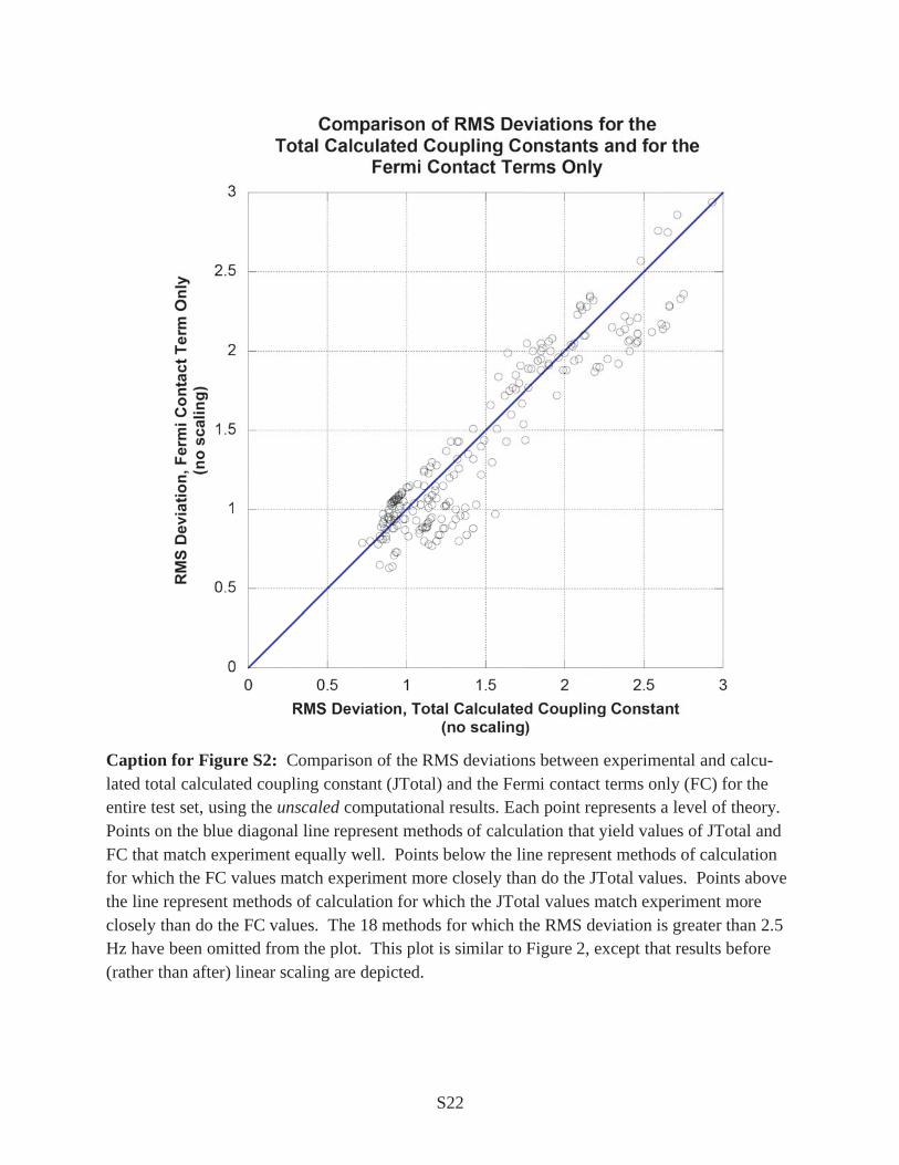
Caption for Figure S2: Comparison of the RMS deviations between experimental and calcu-lated total calculated coupling constant (JTotal) and the Fermi contact terms only (FC) for the entire test set, using the unscaled computational results. Each point represents a level of theory. Points on the blue diagonal line represent methods of calculation that yield values of JTotal and FC that match experiment equally well. Points below the line represent methods of calculation for which the FC values match experiment more closely than do the JTotal values. Points above the line represent methods of calculation for which the JTotal values match experiment more closely than do the FC values. The 18 methods for which the RMS deviation is greater than 2.5 Hz have been omitted from the plot. This plot is similar to Figure 2, except that results before (rather than after) linear scaling are depicted.

S23

Caption for Figure S3: Plot of computed Fermi contact terms versus computed total coupling constants, for the test set (166 total coupling constants), at B3LYP/6-31G(d,p). The calculations were performed in the gas phase, using the “mixed” option, and at the B3LYP/6-31G(d) optimi-zed geometries. The best fit line shown has a correlation coefficient of R2 0.9978, a slope of 1.012, and an intercept of 0.47 Hz. The point for formaldehyde (43.17 Hz, 43.81 Hz) has been omitted from the plot, since including it would compress all the other points on the plot substan-tially.

S24

Table S2a. Effect of including geometry reoptimization for the test set (deviations in Hz). a) Basis Set Jtotal b)

AAD d) Jtotal b)

RMSDe) Jtotal b)

MaxDf) FConly c)

AAD d) FConly c)

RMSDe) FConly c)

MaxDf)

6-31G(d,p) 0.02 0.03 0.18 0.02 0.03 0.20 6-31+G(d,p) 0.07 0.12 0.69 0.07 0.13 0.69 6-311G(d,p) 0.07 0.12 0.89 0.07 0.12 0.91 6-311++G(d,p) 0.07 0.12 0.86 0.07 0.13 0.91 cc-pVDZ 0.15 0.30 2.48 0.14 0.30 2.45 aug-cc-pVDZ 0.14 0.28 2.28 0.14 0.29 2.34 cc-pVTZ 0.10 0.14 0.56 0.10 0.13 0.59 aug-cc-pVTZ 0.10 0.14 0.59 0.10 0.14 0.64

a) calculations using the “mixed” procedure; deviations in calculated coupling constants relative to calculations using the B3LYP/6-31G(d) geometry; b) calculation of total coupling constants; c) calculation of Fermi-Contact terms only; d)AAD = average absolute deviation; e)

RMSD = root mean square deviation; f)MaxD = maximum (absolute) deviation.

Table S2b. Effect of including geometry reoptimization for the test set (deviations in Hz). a)

Basis Set Jtotal b)

AAD d) Jtotal b)

RMSDe) Jtotal b)

MaxDf) FConly c)

AAD d) FConly c)

RMSDe) FConly c)

MaxDf)

6-31G(d,p) 0.02 0.03 0.16 0.02 0.03 0.18 6-31+G(d,p) 0.06 0.10 0.59 0.06 0.11 0.60 6-311G(d,p) 0.06 0.09 0.71 0.06 0.09 0.73 6-311++G(d,p) 0.06 0.10 0.72 0.06 0.10 0.77 cc-pVDZ 0.11 0.21 1.79 0.10 0.21 1.75 aug-cc-pVDZ 0.09 0.20 1.68 0.09 0.21 1.74 cc-pVTZ 0.08 0.11 0.54 0.08 0.11 0.58 aug-cc-pVTZ 0.09 0.12 0.59 0.08 0.12 0.64

a) calculations not using the “mixed” procedure; deviations in calculated coupling constants relative to calculations using the B3LYP/6-31G(d) geometry; b) calculation of total coupling constants; c) calculation of Fermi-Contact terms only; d)AAD = average absolute deviation; e)

RMSD = root mean square deviation; f)MaxD = maximum (absolute) deviation.

S25

Table S3a. Effect of including chloroform as solvent on calculated coupling constants for the test set (deviations in Hz). a)

Basis Set Jtotal b)

AAD d) Jtotal b)

RMSDe) Jtotal b)

MaxDf) FCony c)

AAD c) RMSDe) FConly c)

FConly c)

MaxDf) 6-31G(d,p) 0.10 0.22 1.63 0.10 0.22 1.63 6-31+G(d,p) 0.10 0.22 1.59 0.10 0.22 1.60 6-311G(d,p) 0.11 0.24 1.63 0.11 0.24 1.65 6-311++G(d,p) 0.10 0.21 1.52 0.10 0.22 1.54 cc-pVDZ 0.07 0.17 1.30 0.07 0.17 1.31 aug-cc-pVDZ 0.08 0.17 1.28 0.08 0.17 1.29 cc-pVTZ 0.09 0.21 1.50 0.09 0.21 1.52 aug-cc-pVTZ 0.10 0.23 1.65 0.10 0.23 1.67

a) calculations using the “mixed” procedure, and not including geometry reoptimization; deviations in calculated coupling constants relative to a corresponding gas-phase calculation; b) calculation of total coupling constants; c) calculation of Fermi-Contact terms only; d)AAD = average absolute deviation; e) RMSD = root mean square deviation; f)MaxD = maximum (absolute) deviation.

Table S3b. Effect of including choroform as solvent on calculated coupling constants for the test set (deviations in Hz). a)

Basis Set JTotal b)

AAD d) JTotal b)

RMSDe) JTotal b)

MaxD f) FC c)

AAD c) FC c)

RMSDe) FC c)

MaxD f)

6-31G(d) 0.10 0.24 1.85 0.10 0.23 1.83 6-31G(d,p) 0.10 0.23 1.81 0.10 0.23 1.81 6-31+G(d,p) 0.11 0.25 2.12 0.11 0.25 2.11 6-311G(d,p) 0.10 0.22 1.54 0.10 0.22 1.56 6-311++G(d,p) 0.10 0.23 1.68 0.10 0.23 1.69 cc-pVDZ 0.08 0.20 1.71 0.08 0.20 1.70 aug-cc-pVDZ 0.08 0.19 1.59 0.08 0.19 1.59 cc-pVTZ 0.10 0.23 1.73 0.10 0.23 1.75 aug-cc-pVTZ 0.10 0.24 1.82 0.10 0.24 1.83

a) calculations using the “mixed” procedure, and including geometry reoptimization; deviations in calculated coupling constants relative to a corresponding gas-phase calculation; b) calculation of total coupling constants; c) calculation of Fermi-Contact terms only; d)AAD = average absolute deviation; e) RMSD = root mean square deviation; f)MaxD = maximum (absolute) deviation.

S26

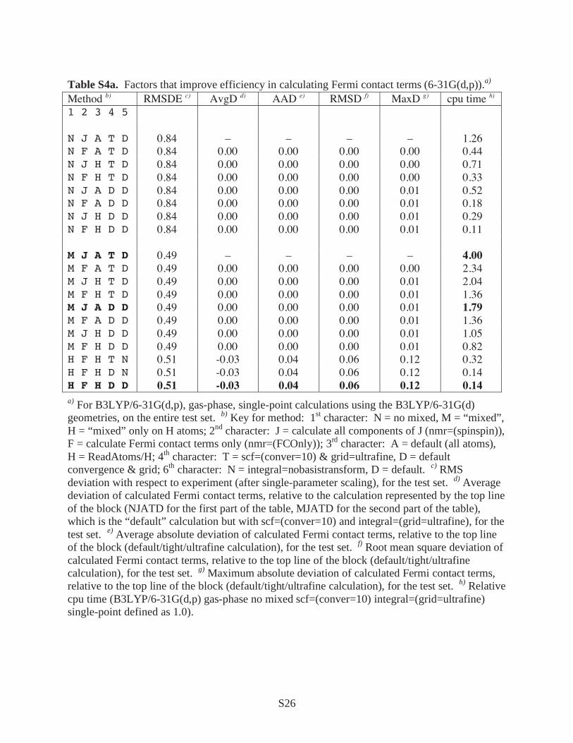
Table S4a. Factors that improve efficiency in calculating Fermi contact terms (6-31G(d,p)).a) Method b) RMSDE c) AvgD d) AAD e) RMSD f) MaxD g) cpu time h) 1 2 3 4 5 N J A T D 0.84 – – – – 1.26 N F A T D 0.84 0.00 0.00 0.00 0.00 0.44 N J H T D 0.84 0.00 0.00 0.00 0.00 0.71 N F H T D 0.84 0.00 0.00 0.00 0.00 0.33 N J A D D 0.84 0.00 0.00 0.00 0.01 0.52 N F A D D 0.84 0.00 0.00 0.00 0.01 0.18 N J H D D 0.84 0.00 0.00 0.00 0.01 0.29 N F H D D 0.84 0.00 0.00 0.00 0.01 0.11 M J A T D 0.49 – – – – 4.00 M F A T D 0.49 0.00 0.00 0.00 0.00 2.34 M J H T D 0.49 0.00 0.00 0.00 0.01 2.04 M F H T D 0.49 0.00 0.00 0.00 0.01 1.36 M J A D D 0.49 0.00 0.00 0.00 0.01 1.79 M F A D D 0.49 0.00 0.00 0.00 0.01 1.36 M J H D D 0.49 0.00 0.00 0.00 0.01 1.05 M F H D D 0.49 0.00 0.00 0.00 0.01 0.82 H F H T N 0.51 -0.03 0.04 0.06 0.12 0.32 H F H D N 0.51 -0.03 0.04 0.06 0.12 0.14 H F H D D 0.51 -0.03 0.04 0.06 0.12 0.14 a) For B3LYP/6-31G(d,p), gas-phase, single-point calculations using the B3LYP/6-31G(d) geometries, on the entire test set. b) Key for method: 1st character: N = no mixed, M = “mixed”, H = “mixed” only on H atoms; 2nd character: J = calculate all components of J (nmr=(spinspin)), F = calculate Fermi contact terms only (nmr=(FCOnly)); 3rd character: A = default (all atoms), H = ReadAtoms/H; 4th character: T = scf=(conver=10) & grid=ultrafine, D = default convergence & grid; 6th character: N = integral=nobasistransform, D = default. c) RMS deviation with respect to experiment (after single-parameter scaling), for the test set. d) Average deviation of calculated Fermi contact terms, relative to the calculation represented by the top line of the block (NJATD for the first part of the table, MJATD for the second part of the table), which is the “default” calculation but with scf=(conver=10) and integral=(grid=ultrafine), for the test set. e) Average absolute deviation of calculated Fermi contact terms, relative to the top line of the block (default/tight/ultrafine calculation), for the test set. f) Root mean square deviation of calculated Fermi contact terms, relative to the top line of the block (default/tight/ultrafine calculation), for the test set. g) Maximum absolute deviation of calculated Fermi contact terms, relative to the top line of the block (default/tight/ultrafine calculation), for the test set. h) Relative cpu time (B3LYP/6-31G(d,p) gas-phase no mixed scf=(conver=10) integral=(grid=ultrafine) single-point defined as 1.0).

S27

Table S4b. Factors that improve efficiency in calculating Fermi contact terms (6-311G(d,p)).a) Method b) RMSDE c) AvgD d) AAD e) RMSD f) MaxD g) cpu time h) 1 2 3 4 5 N J A T D 0.84 – – – – 2.15 N F A T D 0.84 0.00 0.00 0.00 0.00 0.70 N J H T D 0.84 0.00 0.00 0.00 0.00 1.09 N F H T D 0.84 0.00 0.00 0.00 0.00 0.41 N J A D D 0.84 0.00 0.00 0.00 0.01 0.83 N F A D D 0.84 0.00 0.00 0.00 0.01 0.28 N J H D D 0.84 0.00 0.00 0.00 0.01 0.47 N F H D D 0.84 0.00 0.00 0.00 0.01 0.17 M J A T D 0.53 – – – – 4.70 M F A T D 0.53 0.00 0.00 0.00 0.00 3.19 M J H T D 0.53 0.00 0.00 0.00 0.01 2.95 M F H T D 0.53 0.00 0.00 0.00 0.01 1.81 M J A D D 0.53 0.00 0.00 0.00 0.01 2.27 M F A D D 0.53 0.00 0.00 0.00 0.01 1.73 M J H D D 0.53 0.00 0.00 0.00 0.01 1.34 M F H D D 0.53 0.00 0.00 0.00 0.01 1.08 H F H T N 0.53 0.01 0.01 0.02 0.12 0.74 H F H D N 0.53 0.01 0.01 0.02 0.12 0.23 H F H D D 0.53 0.01 0.01 0.02 0.12 0.31 a) For B3LYP/6-311G(d,p), gas-phase, single-point calculations using the B3LYP/6-31G(d) geometries, on the entire test set. b) Key for method: 1st character: N = no mixed, M = “mixed”, H = “mixed” only on H atoms; 2nd character: J = calculate all components of J (nmr=(spinspin)), F = calculate Fermi contact terms only (nmr=(FCOnly)); 3rd character: A = default (all atoms), H = ReadAtoms/H; 4th character: T = scf=(conver=10) & grid=ultrafine, D = default convergence & grid; 6th character: N = integral=nobasistransform, D = default. c) RMS deviation with respect to experiment (after single-parameter scaling), for the test set. d) Average deviation of calculated Fermi contact terms, relative to the calculation represented by the top line of the block (NJATD for the first part of the table, MJATD for the second part of the table), which is the “default” calculation but with scf=(conver=10) and integral=(grid=ultrafine), for the test set. e) Average absolute deviation of calculated Fermi contact terms, relative to the top line of the block (default/tight/ultrafine calculation), for the test set. f) Root mean square deviation of calculated Fermi contact terms, relative to the top line of the block (default/tight/ultrafine calculation), for the test set. g) Maximum absolute deviation of calculated Fermi contact terms, relative to the top line of the block (default/tight/ultrafine calculation), for the test set. h) Relative cpu time (B3LYP/6-31G(d,p) gas-phase no mixed scf=(conver=10) integral=(grid=ultrafine) single-point defined as 1.0).

S28

Table S4c. Factors that improve efficiency in calculating Fermi contact terms (cc-pVTZ).a) Method b) RMSDE c) AvgD d) AAD e) RMSD f) MaxD g) cpu time h) 1 2 3 4 5 N J A T D 0.51 – – – – 8.55 N F A T D 0.51 0.00 0.00 0.00 0.00 3.03 N J H T D 0.51 0.00 0.00 0.00 0.00 5.28 N F H T D 0.51 0.00 0.00 0.00 0.00 2.01 N J A D D 0.51 0.00 0.00 0.00 0.01 4.87 N F A D D 0.51 0.00 0.00 0.00 0.01 1.52 N J H D D 0.51 0.00 0.00 0.00 0.01 3.00 N F H D D 0.51 0.00 0.00 0.00 0.01 1.04 M J A T D 0.51 – – – – 22.99 M F A T D 0.51 0.00 0.00 0.00 0.00 12.03 M J H T D 0.51 0.00 0.00 0.00 0.01 13.81 M F H T D 0.51 0.00 0.00 0.00 0.01 8.04 M J A D D 0.51 0.00 0.00 0.00 0.01 11.50 M F A D D 0.51 0.00 0.00 0.00 0.01 8.22 M J H D D 0.51 0.00 0.00 0.00 0.01 8.00 M F H D D 0.51 0.00 0.00 0.00 0.01 5.57 H F H T N 0.51 0.00 0.00 0.01 0.03 3.39 H F H D N 0.51 0.00 0.00 0.01 0.03 1.34 H F H D D 0.51 0.00 0.00 0.01 0.03 1.30 a) For B3LYP/cc-pVTZ, gas-phase, single-point calculations using the B3LYP/6-31G(d) geometries, on the entire test set. b) Key for method: 1st character: N = no mixed, M = “mixed”, H = “mixed” only on H atoms; 2nd character: J = calculate all components of J (nmr=(spinspin)), F = calculate Fermi contact terms only (nmr=(FCOnly)); 3rd character: A = default (all atoms), H = ReadAtoms/H; 4th character: T = scf=(conver=10) & grid=ultrafine, D = default conver-gence & grid; 6th character: N = integral=nobasistransform, D = default. c) RMS deviation with respect to experiment (after single-parameter scaling), for the test set. d) Average deviation of calculated Fermi contact terms, relative to the calculation represented by the top line of the block (NJATD for the first part of the table, MJATD for the second part of the table), which is the “default” calculation but with scf=(conver=10) and integral=(grid=ultrafine), for the test set. e) Average absolute deviation of calculated Fermi contact terms, relative to the top line of the block (default/tight/ultrafine calculation), for the test set. f) Root mean square deviation of calculated Fermi contact terms, relative to the top line of the block (default/tight/ultrafine calculation), for the test set. g) Maximum absolute deviation of calculated Fermi contact terms, relative to the top line of the block (default/tight/ultrafine calculation), for the test set. h) Relative cpu time (B3LYP/6-31G(d,p) gas-phase no mixed scf=(conver=10) integral=(grid=ultrafine) single-point defined as 1.0).