Quantum and Thermal Phase Escape in Extended Josephson Systems · Quantum and Thermal Phase Escape...
170
Quantum and Thermal Phase Escape in Extended Josephson Systems Den Naturwissenschaftlichen Fakult¨ aten der Friedrich-Alexander-Universit¨ at Erlangen-N ¨ urnberg zur Erlangung des Doktorgrades vorgelegt von Alexander Kemp aus Montreal (Kanada)
Transcript of Quantum and Thermal Phase Escape in Extended Josephson Systems · Quantum and Thermal Phase Escape...

Quantum and Thermal PhaseEscape in Extended Josephson
Systems
Den Naturwissenschaftlichen Fakultaten derFriedrich-Alexander-Universitat Erlangen-Nurnberg
zurErlangung des Doktorgrades
vorgelegt vonAlexander Kemp
aus Montreal (Kanada)

Als Dissertation genehmigt von den Naturwissenschaftlichen Fakultaten derUniversitat Erlangen-Nurnberg
Tag der mundlichen Prufung: 12.7.2006
Vorsitzender der Promotionskommission: Prof. Dr. D.-P. Hader
Erstberichterstatter: Prof. Dr. A. V. Ustinov
Zweitberichterstatter: Prof. Dr. N. Pedersen

i

ii

Contents
Preface vii
1 Introduction and Theory 11.1 Superconductivity . . . . . . . . . . . . . . . . . . . . . . . . . 11.2 Small Josephson Junctions . . . . . . . . . . . . . . . . . . . . 41.3 Quasiparticles and the Gap . . . . . . . . . . . . . . . . . . . . 61.4 The RCSJ Model . . . . . . . . . . . . . . . . . . . . . . . . . 81.5 The Two-Dimensional Sine-Gordon Equation . . . . . . . . . . 101.6 Long Josephson Junctions . . . . . . . . . . . . . . . . . . . . 12
1.6.1 Soliton Solutions . . . . . . . . . . . . . . . . . . . . . 151.6.2 Small Wave Excitations . . . . . . . . . . . . . . . . . 151.6.3 Idle Region Effects . . . . . . . . . . . . . . . . . . . . 17
1.7 Annular Junctions . . . . . . . . . . . . . . . . . . . . . . . . . 181.7.1 Perturbation Theory: Vortex Effective Potentials . . . . 221.7.2 Vortex Dynamics . . . . . . . . . . . . . . . . . . . . . 23
2 Experimental Technique and data evaluation 272.1 Measurement Scheme . . . . . . . . . . . . . . . . . . . . . . . 272.2 Vortex Injection . . . . . . . . . . . . . . . . . . . . . . . . . . 282.3 Escape Field Distributions . . . . . . . . . . . . . . . . . . . . 322.4 Thermal Escape in a Washboard Potential . . . . . . . . . . . . 372.5 Damping Regimes . . . . . . . . . . . . . . . . . . . . . . . . 382.6 Parameter Estimation . . . . . . . . . . . . . . . . . . . . . . . 412.7 Conclusion . . . . . . . . . . . . . . . . . . . . . . . . . . . . 42
3 Metastable Vortex States 453.1 Metastable Vortex States . . . . . . . . . . . . . . . . . . . . . 45
iii

3.2 Spectroscopy on an Annular Junction . . . . . . . . . . . . . . 473.3 On Classical Resonances and Quantum Transitions . . . . . . . 503.4 Thermal Activation of a Vortex . . . . . . . . . . . . . . . . . . 543.5 From the Low Damping Regime to the Quantum Regime . . . . 573.6 Crossover to the Small Junction Case . . . . . . . . . . . . . . . 613.7 Conclusion . . . . . . . . . . . . . . . . . . . . . . . . . . . . 68
4 Phase Escape In Extended Systems 714.1 Harmonic Approximation . . . . . . . . . . . . . . . . . . . . . 724.2 VAV Dissociation . . . . . . . . . . . . . . . . . . . . . . . . . 764.3 RF Induced Decay . . . . . . . . . . . . . . . . . . . . . . . . 794.4 Thermal Activation and Quantum Regime . . . . . . . . . . . . 824.5 Conclusion . . . . . . . . . . . . . . . . . . . . . . . . . . . . 85
5 Double-Well Potentials 875.1 Parasitic Potentials . . . . . . . . . . . . . . . . . . . . . . . . 895.2 Lithographic Microshorts . . . . . . . . . . . . . . . . . . . . . 95
5.2.1 Bistable States in Microshort Junctions . . . . . . . . . 995.2.2 Readout . . . . . . . . . . . . . . . . . . . . . . . . . . 1005.2.3 State Preparation . . . . . . . . . . . . . . . . . . . . . 1045.2.4 Experimental Test of State Preparation and Readout . . 1045.2.5 Symmetry of the Patterns . . . . . . . . . . . . . . . . . 1085.2.6 Thermal Activation over a Suppressed Barrier . . . . . . 1095.2.7 Second Order Perturbation . . . . . . . . . . . . . . . . 114
5.3 Discussion . . . . . . . . . . . . . . . . . . . . . . . . . . . . . 117
6 Discussion, conclusions and outlook 119
Summary 121
Zusammenfassung 123
A Biasing 125A.1 Biasing Scheme . . . . . . . . . . . . . . . . . . . . . . . . . . 126A.2 Power Dissipation of the Biasing System . . . . . . . . . . . . . 127
B Electronics 131B.1 Computer Control . . . . . . . . . . . . . . . . . . . . . . . . . 131B.2 Noise Estimation of the Ramp-Type Experiments . . . . . . . . 132
iv

C Table of Samples and Measurements 137C.1 Samples Used . . . . . . . . . . . . . . . . . . . . . . . . . . . 137C.2 Table of Measurements . . . . . . . . . . . . . . . . . . . . . . 137
D Table of variables 141
Bibliography 147
Acknowledgements 155
Curriculum Vitae 159
v

vi
Preface
Since the description of the phenomena on coupled superconductors by Joseph-son [1], the dynamics of the quantum mechanical phase across a Josephson junc-tion (JJ) has been studied extensively. A well known application of these effectsis the superconducting quantum interferometer, which is a sensitive measure-ment device. The JJ in a SQUID is completely described by this single macro-scopic variable, which behaves as a single degree of freedom. In the resistively-capacitively shunted junction model, a resistance acts as a damping element onthis degree of freedom, while the capacitive part represents an effective mass.Because of the nonlinearity of the Josephson element, metastable states can ex-ist. Fluctuations by thermal noise current in the resistive state of the junctionwere described by Dahm et al. [2] Due to this noise current metastable states in asmall junction have a finite lifetime, examined by Fulton et al. [3] and Kukijarviet al. [4]. Recently, Josephson junctions received attention in the context ofquantum computation. The basis for this was set long ago [5, 6, 7] by observingmacroscopic quantum behaviour of the superconducting phase difference.
In long Josephson junctions the soliton solution of the governing sine-Gordon equation corresponds to a circulating vortex of supercurrent. In thiswork thermal, quantum limited and RF induced activation from metastable statesin long, annular Josephson junctions are presented. It is a continuation of the re-search on fluctuation induced activation in annular Josephson junctions done byA. Wallraff [8] which resulted in the experimental observation of macroscopicquantum tunneling of a vortex in sub-µm junctions, described in Ref. [9]. At thisstage, a classical two-state system, formed by heart-shaped Josephson junctionswas demonstrated [10, 11, 12], the use of which as a quantum bit was proposedin Ref. [13]. Hence another direction of research was open at the beginning ofthe work on this thesis.
Quantum tunneling in reproducible µm scale annular junctions is observed,similar to the results given in Ref. [9]. The samples used were of low critical cur-
vii
rent density, and therefore physically shorter, and may behave as short Joseph-son junctions. The measurements presented here answer the following question:May the phase variable in a long Josephson junction tunnel homogeneously,even if it is twisted by a trapped quantum of magnetic flux? Depending on tem-perature and magnetic field a range of behaviours, like thermal vortex activation[14], thermal small junction activation [3], and quantum tunneling [5, 6, 7, 9] isobserved. I interpret the results using a newly developed approximation of thephase distribution in the junction, derived from the one given in Ref. [15], butadapted to a single flux quantum trapped in a short annular Josephson junctionlimit. From the activated escape of the phase I proceed to another type of activa-tion from a metastable state. The vortex-antivortex nucleation process, discussedby Fistul et al. [16], is another approximation of what is described for a shortjunction in Ref. [15].
Of major importance for applications, the parasitic barrier created by thetwo dimensional design of the heart-shaped Josephson junctions was to be de-termined by the means of thermal activation between bistable states. Only thecalculations given in Ref. [17] explain the failure to observe any thermal activa-tion. A changed vortex rest mass, a parasitic effect at strongly curved regions inthe samples used, prohibited any systematic observation of thermal activation inheart-shaped Josephson junctions.
Although this leaves some perspective for an enhanced design of heart-shaped Josephson junctions, another bistable system, namely a microshort junc-tion, seems more attractive. This kind of junction was examined before theo-retically in Ref. [18]. The realization was prevented by the trilayer technologygenerally used for the production of the junctions, which allows for only a singlecritical current density. As a conclusion and a way ahead, we propose a novelproduction technique for microshorts, namely a width modulated junction. Theuse of this mechanism for potential engineering was discussed by Goldobin etal. [19]. The concept of this approach is that a small longitudinal region of thejunction repels the vortex because of its enhanced width. The advantages of thisapproach are, besides the simplicity of the concept, the steepness of the poten-tials generated. Furthermore, it does not require sub-µm sample production, butonly sub-µm level size control, which is within the limits of visible light photo-lithography. Results, including state preparation and readout protocol, will bepublished elsewhere in Ref. [20] and form the last experimental chapter of thisthesis. Measurements done in collaboration with A. Price lead to the observationof quantum tunneling of a vortex through a barrier in a photo-lithographicallyproduced 1 kA/cm2 sample, which will be published elsewhere [21].
viii
Chapter 1
Introduction and Theory
1.1 SuperconductivitySuperconductors were discovered in 1911 by Heike-Kamerlingh Onnes. Belowa critical temperature the resistance of superconductors drops to zero. This effectcould not be explained until Bardeen, Cooper and Schrieffer [22] interpreted thisas electrons of opposite spin1 bound together by phonons, the composite particlebeing similar to a boson. These are formed if the average thermal energy of theelectron bath is low enough and condense into a collective ground state, loweringthe total energy of the system. Any Fermi sea is unstable against this pair for-mation, given an arbitrarily small attractive force between the particles. At finitetemperature elementary excitations on the whole system, called quasiparticlescoexists to the Cooper pairs.
Because this collective ground state behaves as a single quantum particle,it is described by a macroscopic wavefunction. In a bulk superconductor, thereexists no excitation other than a modulation of the phase of this wavefunction2.Thus the system is governed by
Ψ = Ψ0eiφ(~x,t), (1.1)
where |Ψ0|2 is the amplitude of the ground-state wavefunction. The field φ(~x, t)1Superconductors with Cooper pairs of spin 1 exist, called heavy-fermion superconductors.
Cooper pairs in high TC superconductors are also suspected to have another pairing mechanism.2For one and two dimensional superconducting structures, oscillations of the order parameter are
possible, resulting in the existence of phase slip centers in thin wires [23] or phase slip lines in thinfilms [24]
1

2 CHAPTER 1. INTRODUCTION AND THEORY
is the only degree of freedom, if the energy is lower than the energy gap of the su-perconductor. For niobium, the superconductor used in the experiments reportedin this thesis, the energy a single quasiparticle needs to acquire is 1.4 meV. If,at a Josephson junction the available energy per electron exceeds this value, aCooper pair is removed from the ground state wavefunction and broken intoquasiparticles. The amplitude of this wavefunction has a certain value |Ψ0| inthe bulk superconductor, which decays exponentially outside the superconductorwith the coherence length ξ, as shown in Fig. 1.1. Besides the lack of resistance
|Ψ22|
x
| ~H|
λLζ
Figure 1.1: Inside a superconductor, the magnetic field decreases exponentiallyas a function of coordinate x, while outside of the superconductor the amplitudeof the wavefunction decreases exponentially.
there are two features of superconductors deserving a closer look, namely theMeissner effect and the fluxoid quantization.
Magnetic flux is expelled from a bulk piece of superconductor, illustrated inFig. 1.1. This state is called the Meissner state. It turns out that only a thin sur-face layer of the London penetration depth λL carries a current, which compen-sates the external magnetic field inside of the bulk superconductor. Combiningthe second London equation,
~h = −cΛ∇× ~Js, (1.2)
with Ampere’s law yields
∇2 ~Hs =~Hs
λL2 , (1.3)
where ~Js is the density of the supercurrent and the phenomenological parameterΛ given by
Λ =4πλL
c2. (1.4)
1.1. SUPERCONDUCTIVITY 3
Solving this leads to an exponential decay of the magnetic field ~Hs inside thesuperconductor.
The Ginzburg-Landau theory, essentially an expansion of the free energyin the superconductor, describes the essential thermodynamic properties of thesuperconducting-normal phase transition. It can be used to predict that the differ-ence between the coherence length and the London penetration depth determinesthe surface energy between the superconducting and the normal phase inside asuperconductor. While a positive surface energy makes the minimal surface theequilibrium state, a negative surface energy supports the existence of normalconducting regions, separated from each other. These regions appear as separatetreads of magnetic flux through the superconductor, Abrikosov vortices[25]. Su-perconductors with negative surface energy are called type-II superconductors.Niobium, the superconductor, which was used in the experiments presented inthis work, is a type-II superconductor. Without careful magnetic shielding thesuperconductor is not in the Meissner state, but in a mixed state, a state firstobserved by Shubnikov et al.[26].
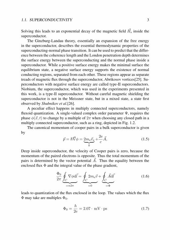
A peculiar effect happens in multiply connected superconductors, namelyfluxoid quantization. A single-valued complex order parameter Ψ, requires thephase φ(~x, t) to change by a multiple of 2π when choosing any closed path in amultiply connected superconductor, such as a ring, depicted in Fig. 1.2.
The canonical momentum of cooper pairs in a bulk superconductor is givenby
~p = ~~∇φ = 2me~vs︸ ︷︷ ︸0
+2ec
~A, (1.5)
Deep inside superconductor, the velocity of Cooper pairs is zero, because themomentum of the paired electrons is opposite. Thus the total momentum of thepairs is determined by the vector potential ~A. Thus the equality between theenclosed flux Φ and the integral value of the phase gradient,
Φ0
2π
∮C
∇φd~l︸ ︷︷ ︸=n2π
=∮
C
2me~v︸ ︷︷ ︸=0
+∮
C
~Ad~l︸ ︷︷ ︸=Φ
(1.6)
leads to quantization of the flux enclosed in the loop. The values which the fluxΦ may take are multiples Φ0.
Φ0 =h
2e= 2.07 · mV · ps (1.7)

4 CHAPTER 1. INTRODUCTION AND THEORY
C
Φ = Φ0n
Figure 1.2: Themagnetic flux Φin a closed super-conducting loopof a thicknessmuch larger thanthe coherencelength ξ of thesuperconductoris restricted to amultiple of Φ0.
1.2 Small Josephson Junctions
The Josephson effect was first predicted in 1962 by Josephson [1], and observedby Anderson and Roswell [27]. It occurs in a tunnel junction, in which the cur-rent across the tunneling barrier is carried by a supercurrent of Cooper pairs.Ambegaokar and Baratoff[28] analysed the tunneling processes including thetemperature dependence and a relation between the normal resistance and thecritical current of a tunnel barrier. Different types of weak links, such as nar-row superconducting bridges between superconductors, or thin layers of normalmetal or an insulator can act as barrier to Cooper pairs. In the experiments re-ported in this thesis only the latter type of junction was used. The wavefunctionsof the two electrodes extend beyond the length scale of the coherence length ofthe order parameter, illustrated in Fig. 1.3.
There are two important relations, which relate the difference ϕ = φ1−φ2 ofthe phases of the superconducting wavefunctions to the current and to the voltageacross the barrier. In calculating the overlap integral explicitly, the coupling

1.2. SMALL JOSEPHSON JUNCTIONS 5
Superconductor
Insulator
Superconductor|Ψ22|
I
|Ψ21| Figure 1.3: Over-
lap of the wave-functions Ψ1 andΨ2 causes a fi-nite coupling en-ergy. A currentI would cause aphase differencebetween the twoelectrodes.
energy is written as
HJ = −∫
Ω
[(Ψ∗1Ψ2 + Ψ∗
2Ψ1)]dΩ, (1.8)
where Ω is the region of overlapping wavefunctions.This yields the phase dependent coupling energy
HJ = −EJ cos ϕ (1.9)
where EJ is the coupling energy for zero phase difference. From this[29], theDC Josephson relation
I = IC sinϕ (1.10)
can be derived. The critical current IC of the weak link is proportional to thecoupling energy:
IC = EJ2π
Φ0. (1.11)
If transport current exceeds the critical current, a voltage drop appears across theweak link. The AC Josephson relation relates the time derivative ϕt to the DCvoltage V between the two electrodes:
V = ϕtΦ0
2π. (1.12)
Combining this with Eq. (1.10), yields a time dependent supercurrent
I = IC sin(
ϕ0 + tV2π
Φ0
). (1.13)

6 CHAPTER 1. INTRODUCTION AND THEORY
The frequency ν is given by
ν = V1
Φ0. (1.14)
A real Josephson junction is described by the RCSJ model, discussed below, inwhich the ac current causes an ac voltage across the junction.
1.3 Quasiparticles and the Gap
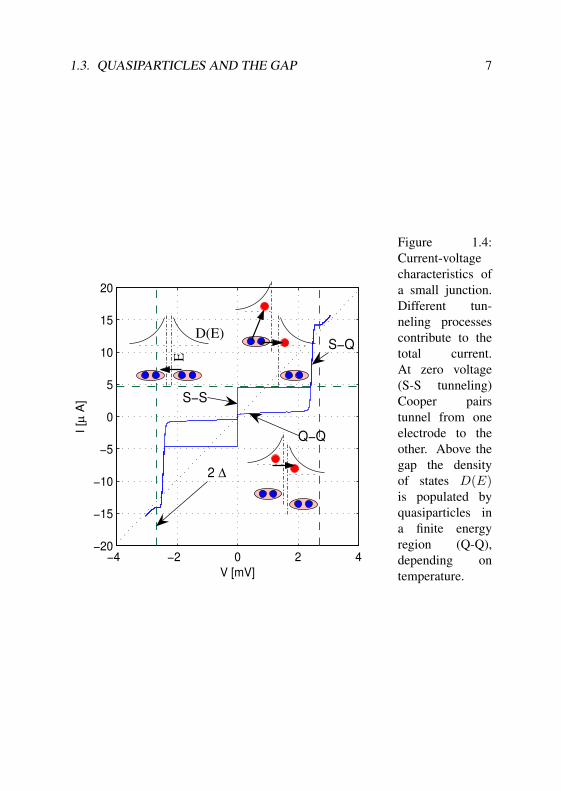
The current-voltage characteristics for both, zero and non-zero voltage is plottedin Fig. 1.4. In Ref. [30] the different processes leading to this picture are dis-cussed on a microscopic model. In the zero-voltage state the current is carriedby the non-resistive Cooper pair tunneling. At 2∆G enough energy is availableto break a Cooper pair and inject one of the generated quasiparticles into theother electrodes quasiparticle band. At voltages below 2∆G only quasiparticlesalready excited by temperature are available to carry the current. Setting up theequations of motion for ϕ is done using the resistively-capacitively shunted junc-tion (RCSJ) model shown in Fig. 1.5, where a Josephson junction is representedby a Josephson element fulfilling the DC Josephson relation, a capacitor repre-senting the junction capacitance and a resistor, which represents the dissipativequasiparticle current.
The quasiparticle resistance plays a fundamental role in the thermal activa-tion processes discussed later. It is the schematic, lumped element representa-tion of the coupling of the superconducting order parameter to the heat bath.Around zero voltage (same chemical potential for quasiparticles on both sides)quasiparticles are only excited by the thermal energy. This follows the simpleexponential behavior:
Rj = R0 exp∆G(T )TkB
, (1.15)
R0 being the normal resistance, when all current is carried by quasiparticles. Atlow temperatures, ∆G can be assumed constant, otherwise approximated[28, 31]by different phenomenological formulas resembling the value calculated fromthe BCS theory.
1.3. QUASIPARTICLES AND THE GAP 7
−4 −2 0 2 4−20
−15
−10
−5
0
5
10
15
20
V [mV]
I [µ
A] S−S
S−Q
Q−Q
2 ∆
E
D(E)
Figure 1.4:Current-voltagecharacteristics ofa small junction.Different tun-neling processescontribute to thetotal current.At zero voltage(S-S tunneling)Cooper pairstunnel from oneelectrode to theother. Above thegap the densityof states D(E)is populated byquasiparticles ina finite energyregion (Q-Q),depending ontemperature.
8 CHAPTER 1. INTRODUCTION AND THEORY
I
φ1
φ2
UCR IJ
(1)
(2)
ϕ
m
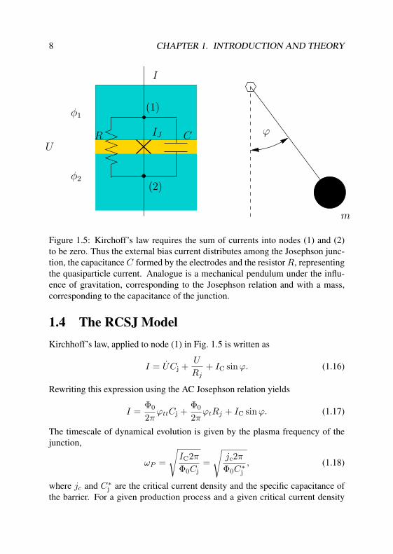
Figure 1.5: Kirchoff’s law requires the sum of currents into nodes (1) and (2)to be zero. Thus the external bias current distributes among the Josephson junc-tion, the capacitance C formed by the electrodes and the resistor R, representingthe quasiparticle current. Analogue is a mechanical pendulum under the influ-ence of gravitation, corresponding to the Josephson relation and with a mass,corresponding to the capacitance of the junction.
1.4 The RCSJ ModelKirchhoff’s law, applied to node (1) in Fig. 1.5 is written as
I = UCj +U
Rj+ IC sinϕ. (1.16)
Rewriting this expression using the AC Josephson relation yields
I =Φ0
2πϕttCj +
Φ0
2πϕtRj + IC sinϕ. (1.17)
The timescale of dynamical evolution is given by the plasma frequency of thejunction,
ωP =
√IC2π
Φ0Cj=
√jc2π
Φ0C∗j
, (1.18)
where jc and C∗j are the critical current density and the specific capacitance of
the barrier. For a given production process and a given critical current density
1.4. THE RCSJ MODEL 9
the plasma frequency is independent of the junction size. Using ωP , Eq. (1.17)is rewritten to
−ϕtt1
ωP2
= sinϕ− γ + α1
ωPϕt, (1.19)
as equation of motion for ϕ, where γ = I/IC and α = 1/(RjCjωP ). The roleof the current I is a driving force on the variable ϕ; α is a damping parame-ter. Johnson noise is omnipresent in resistive electrical circuits [32, 33, 34]as a consequence of the dissipation-fluctuation theorem. Therefore the parallelresistance to the junction also acts as a Gaussian current noise source. It can bedefined most intuitively by the relation between resistance, temperature, obser-vation bandwidth and RMS value.
In =
√4kBTνBW
Rj(1.20)
The time scale can be normalized as
t = tωP−1, (1.21)
so that Eq. (1.19) takes the form
−ϕtt = sinϕ− γ + αϕt. (1.22)
Neglecting the quasiparticle damping by setting α to zero, this system is aHamiltonian system with the equivalent Hamiltonian
H = (1− cos ϕ) +12ϕt
2 − γϕ (1.23)
The energy scale EJ of this Hamiltonian is given by Eq. (1.11)The dynamics of a small junction in presence of quantum or thermal fluc-
tuations, is more conveniently described after defining ~j = ~ωP /EJ to be thenormalized Planck constant and kB,j = kB/EJ to be the normalized Boltzmannconstant. Rewriting ~j in terms of jc and the junction area A,
~j =~A
√(2π
Φ0
)3 1jcC∗
j
(1.24)
shows that for a given junction fabrication process, the only way to increase ~j
is to decrease the junction area.

10 CHAPTER 1. INTRODUCTION AND THEORY
1.5 The Two-Dimensional Sine-Gordon Equation
In an extended junction, such as illustrated in Fig. 1.6, supercurrent flows par-allel to the Josephson barrier in the presence of a magnetic field. Taking intoaccount that the magnetic flux in an inductive region corresponds to the productof the inductance and the current flowing, we use Eq. (1.6) and follow the dashedpath, in Fig. 1.6. The phase gradient from points (1) to (2) and points (3) to (4)does not play a role due to the small thickness of this layer. If the path is chosendeep inside the electrodes we find the identity
(φ1 − φ2)− (φ3 − φ4) =2π
Φ0(Φext − L∗~jinp(x2 − x1)), (1.25)
where L∗ denotes the sheet inductance
L∗ = µ0d′, (1.26)
~jinp the in-plane supercurrent density (Unit is A/m) in the x-direction, and Φext
the externally applied magnetic flux. The magnetic thickness d′ is given byd′ = tJ + 2λL, where tJ is the thickness of the insulating barrier. Lettingthe distance over which the integration is carried out go to zero yields the firstderivative ϕx
ϕx =2π
Φ0(Hextµ0d
′ − L∗~jinp) (1.27)
Generalizing this to two dimensions, where ~Hext,V consists of two in-plane com-ponents of the external magnetic field yields,
∇ϕ =2π
Φ0((~z × ~Hext,V)µ0d
′ − L∗~jinp). (1.28)
The supercurrent in the plane is given by
L∗~jinp = (~z × ~Hext,V)µ0d′ − Φ0
2π∇ϕ. (1.29)
Without an additional source of current, charge conservation in the sheet requiresthat
L∗ ÷~jinp = ∇(~z × ~Hext,V)µ0d′ − Φ0
2π∇2ϕ = 0. (1.30)

1.5. THE TWO-DIMENSIONAL SINE-GORDON EQUATION 11
φ2
φ1
φ3
φ4
2λL + tJ
~x
~y
dΦ
γ
~z
Figure 1.6: In a two-dimensional Josephson junction, the Josephson current andthe displacement current act as local sources in the superconducting plane. Thethickness of the barrier (bright) is not to scale. The dotted lines indicate the mag-netic thickness, which is the barrier thickness plus twice the London penetrationdepth.
Using Kirchhoff’s current law, the Josephson current, the displacement cur-rent, the quasiparticle current, and the external bias current γjc are added3 to thecurrent corresponding to Eq. (1.30). This yields:
Φ0
2π
1L∗∇2ϕ+∇(~z× ~Hext,V) = jc sinϕ+
Φ0
2πC∗
j ϕtt +γjc +1
R∗Φ0
2πϕt, (1.31)
where R∗ is the specific quasiparticle resistance.This equation has a characteristic length scale, the Josephson length λJ ,
which is given by
λJ =
√Φ0
2πL∗jc. (1.32)
Normalizing the spatial coordinates to λJ by defining the normalized co-ordinate x = x/λJ and the time as in Eq. (1.21) yields the two-dimensionalsine-Gordon equation in normalized units
∆ϕ− ϕtt = sinϕ− γ + ∇~hext,V + αϕt, (1.33)
3The surface impedance term, related to the AC voltage induced along the Josephson junction,only plays a role for high fluxon velocities and is neglected here.

12 CHAPTER 1. INTRODUCTION AND THEORY
where ∆ and ∇ denote the corresponding operators acting on normalized units,and hext is the normalized magnetic field, defined by
~hext,V = (~z × ~Hext,V)/H0, H0 =Φ0
2πd′λJµ0. (1.34)
Typical values for H0 are on the order of one gauss for the samples used. (seeAppendix appendix C). Eq. (1.33) can be solved numerically or in the spe-cial case of a long junction be reduced to an one-dimensional model, where allproperties of the junction are described as a function of the position along thejunction. The electromagnetic wave propagation velocity (Swihart velocity) isgiven by
c =λJ
ωP(1.35)
1.6 Long Josephson JunctionsIf the transverse dimension is smaller that the Josephson length λJ and the lon-gitudinal dimension is larger than the Josephson length, then we are dealing withthe special case of a long junction. Long Josephson junctions (LJJ) have receiveda lot of attention as an ideal model system for the one-dimensional sine-Gordonequation. Comprehensive overviews are given in Refs. [35, 36, 37, 38].
The reduction of the dimensionality takes place by assuming that ∆ϕ canbe replaced by ϕxx, where x denotes the coordinate along the junction, alongthe vector ~x, furthermore that ∇~hext,V can be replaced by ∂hy/∂x. This isjustified, if the width in y-direction is sufficiently smaller than the Josephsonlength. In this limit, the currents perpendicular to the longitudinal axis are as-sumed to be zero. This results in a one-dimensional transmission line model, asshown in Fig. 1.7, where the junction electrode is represented by a inductance.Furthermore this approximation requires that the functional determinant of thetransformation from the junction coordinate system to the laboratory system isclose to one, which essentially limits this approximation to junctions where thecurvature of longitudinal axis is sufficiently small[17]. This condition is violatedin the heart-shaped Josephson junctions[13], as discussed in sec. 5.1. After thesimplifications, the one-dimensional sine-Gordon equation takes the form:
ϕxx − ϕtt = sinϕ− γ +∂hext
∂x− αϕt. (1.36)
For the α = 0 case the system is Hamiltonian. The case of zero bias current and

1.6. LONG JOSEPHSON JUNCTIONS 13
IL ∝ ϕx
ϕ(x1) ϕ(x2) ϕ(x3) ϕ(x4)
Figure 1.7: An equivalent lumped element electrical circuit is for a long Joseph-son junction. The central assumption is, that the phase difference in Fig. 1.6between the upper and lower electrode is the equal at both transversal edges ofthe junction y1 and y2. Hence the system can then represented by a inductance-Josephson transmission line along the JJ, carrying a current proportional to thelongitudinal phase gradient.
zero external magnetic field
ϕxx − ϕtt = sinϕ (1.37)
is called the unperturbed sine-Gordon equation.The Hamiltonian consists of the Josephson energy,
HJ =∫ w
0
∫ l
0
(1− cos ϕ) dxdy, (1.38)
the inductive energy
HL =∫ w
0
∫ l
0
12ϕx
2 dxdy, (1.39)
the capacitive energy,
HC =∫ w
0
∫ l
0
12ϕt
2 dxdy, (1.40)
an energy term describing the driving force of the bias current
Hγ = −∫ w
0
∫ l
0
ϕγ dxdy (1.41)

14 CHAPTER 1. INTRODUCTION AND THEORY
and the interaction with the magnetic field
HH =∫ w
0
∫ l
0
ϕ∂hext
∂xdxdy. (1.42)
The total Hamiltonian
H(ϕ, ϕt) = HJ +HL +HC +Hγ +HH (1.43)
can be used for deriving effective potentials using perturbation theory. Assumingconstant width w, Eq. (1.43) is written as4
H(ϕ, ϕt) = w(hext(0)ϕ(0)− hext(l)ϕ(l))+
w
∫ l
0
(12ϕx
2 +12ϕt
2 + ϕγ + ϕxhext − cos ϕ
)dx (1.44)
If the assumption of a homogeneous junction is weakly violated, but the widthof the junction is smaller than λJ it is possible to assume ϕ to be constant in they direction. I use this later to derive the potentials for changing width and finiteradii.
The energy scale E0 of this Hamiltonian is given by
E0 =Φ0
2πwλJ = EJ
1l, (1.45)
the Josephson energy of a small junction of width w and length λJ . Togetherwith the time normalization, this results in a normalized Planck’s constant for aLJJ Hamiltonian
~ =~E0
ωP = ~jl (1.46)
and a normalized Boltzmann constant
kB =kB
E0= kB,jl. (1.47)
The difference from Eq. (1.24) is that reducing the minimum feature size in alithographic process only reduces the width, while the length scale is set by theJosephson length. Therefore the minimum feature size enters in the power −1instead of −2.
4Integration by parts

1.6. LONG JOSEPHSON JUNCTIONS 15
1.6.1 Soliton SolutionsFor the time-independent (static) case without magnetic field and bias currentEq. (1.36) is reduced to the Ferrell-Prange equation:
ϕxx = sinϕ. (1.48)
For infinitely long systems there exist soliton solutions
ϕf(x, x0) = ±4 arctan(ex−x0
), (1.49)
where x0 is the center of mass position of the excitation. The correspondingphase profile is plotted in Fig. 1.8a. A two-dimensional plot of the energy densityof the position and phase dependent terms of Eq. (1.43), as depicted in Fig. 1.9visualizes that the solution ϕf corresponds to a chain connecting one Peierlsvalley [39] to another.
1.6.2 Small Wave ExcitationsSmall amplitude perturbations around a static state ϕ0(x) are possible. Theansatz
ϕ(x, t) = ϕ0(x) + ϕδ(x, t), (1.50)
placed in Eq. (1.36) yields, at zero dissipation:
ϕ0xx + ϕδxx − ϕδtt = sin(ϕ0 + ϕδ). (1.51)
For small amplitude fluctuations ϕδ this takes the form
ϕ0xx + ϕδxx − ϕδtt = sinϕ0 + ϕδ cos ϕ0, (1.52)
which after subtracting the Ferrel-Prange equation reads
ϕδxx − ϕδtt = ϕδ cos ϕ0. (1.53)
Rewriting leads to
−ϕδtt = ϕδ cos(ϕ0)− ϕδxx. (1.54)
Since this is a linear differential equation, the general solution takes the form
ϕδ =N∑
i=1
Ai exp(ωit)ϕδi(x), (1.55)
ϕδi being the eigenmodes of Eq. (1.54) and Ai the amplitude of the small waves.

16 CHAPTER 1. INTRODUCTION AND THEORY
0
0.5
1
1.5
2
ϕ/π
(a)
−10 −5 0 5 100
0.5
1
1.5
2(b)
Position xϕ
x
Figure 1.8: (a) The phase profile of a vortex located at xN = 0, (b) the magneticfield in the barrier (normalized).
Plasmons
Small waves in a homogeneous long Josephson junctions are called plasmons.The constant choice ϕ0 = 0 yields
ϕδxx − ϕδtt = ϕδ, (1.56)
an inhomogeneous wave equation. The solutions
ϕδ(k, ω0(k)) = exp(ı(kx− ω0(k)t)) (1.57)
of this are small amplitude sinusoidal waves. The dispersion relation ω02(k) =
1 + k2 is graphed in Fig. 1.10 for an infinitely long Josephson junction. Modesof frequencies ω < 1 correspond to evanescent modes in a waveguide or lowfrequency waves reflected upon incidence with a plasma. The transmission ofenergy via such modes drops exponentially with the length of the system, asknown from textbooks[40], with a damping constant of αplasma = 2ωP
c . Innormalized units, αplasma = 2, corresponding to an attenuation of 8.7dB per

1.6. LONG JOSEPHSON JUNCTIONS 17
−10
−5
0
5
10
0
1
−1
0
1
2
Position x
Peierls valley Nr.
H
Figure 1.9: The vortex phase profile connects Peierls valley 0 with Peierls valley1. For infinite or annular systems, this defines the solution sector topologically.
Josephson length. For a homogeneously biased Josephson junction ϕ0 takesthe value arcsin γ, and the cutoff frequency as well as the damping constantare changed. Nonlinear PDE simulations of LJJs embedded in superconductingcircuits[41], to evaluate the use as tunable filters for qubit control, verify thescaling of the filter properties with the bias current.
1.6.3 Idle Region Effects
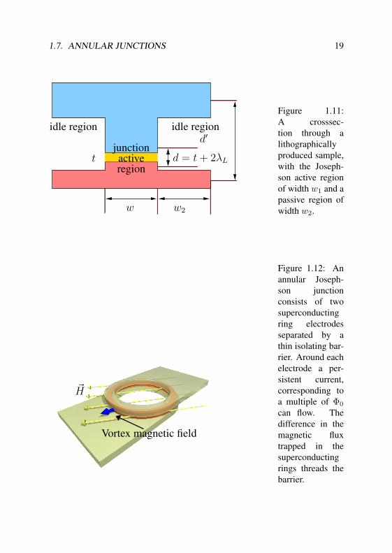
The long junctions used in this work were produced using trilayer technology.Due to limited resolution of photo lithography the junctions have a passive re-gion, as depicted in Fig. 1.11. The junction itself has an active region of widthw, and electrodes outside the junction of width w2. Such junctions have beendiscussed in Refs. [42, 43]. The effective inductance per unit length is in this

18 CHAPTER 1. INTRODUCTION AND THEORY
0 5 100
2
4
6
8
10
k
ω0/ω
P Figure 1.10: Thespectrum ω0(k)for plasmon ex-citations. Thecase k = 0 cor-responds to ahomogeneouslyoscillating junc-tion.
case not given by the sheet inductance, divided by the width but rather by
L∗eff = L∗1
2w2dwd′ + 1
. (1.58)
A detailed experimental investigation of these effects was presented in Ref. [44].The idle region leads to an increase of the Josephson length λJ to an effectivevalue of
λeff = λJ
√1 + 2
w2d
wd′. (1.59)
1.7 Annular JunctionsOne particular geometry of Josephson junctions is the annular geometry, illus-trated in Fig. 1.12 and schematized in Fig. 1.13. The flux quantization allowsthe change of the superconducting phase ϕ around an annular junction circum-ference to be a multiple of 2π only. This imposes a special kind of boundarycondition on annular junctions. The difference in the number of trapped fluxquanta in the upper and lower superconducting ring is called the vorticity nv. Interms of nv the boundary conditions between the phases at position 0 and l takethe form
2πnv = ϕ(l)− ϕ(0) (1.60)
1.7. ANNULAR JUNCTIONS 19
d = t + 2λL
d′
w w2
idle regionidle region
activeregion
junctiont
Figure 1.11:A crosssec-tion through alithographicallyproduced sample,with the Joseph-son active regionof width w1 and apassive region ofwidth w2.
~H
Vortex magnetic field
Figure 1.12: Anannular Joseph-son junctionconsists of twosuperconductingring electrodesseparated by athin isolating bar-rier. Around eachelectrode a per-sistent current,corresponding toa multiple of Φ0
can flow. Thedifference in themagnetic fluxtrapped in thesuperconductingrings threads thebarrier.
20 CHAPTER 1. INTRODUCTION AND THEORY
P
nv2π
· · ·
· · ·
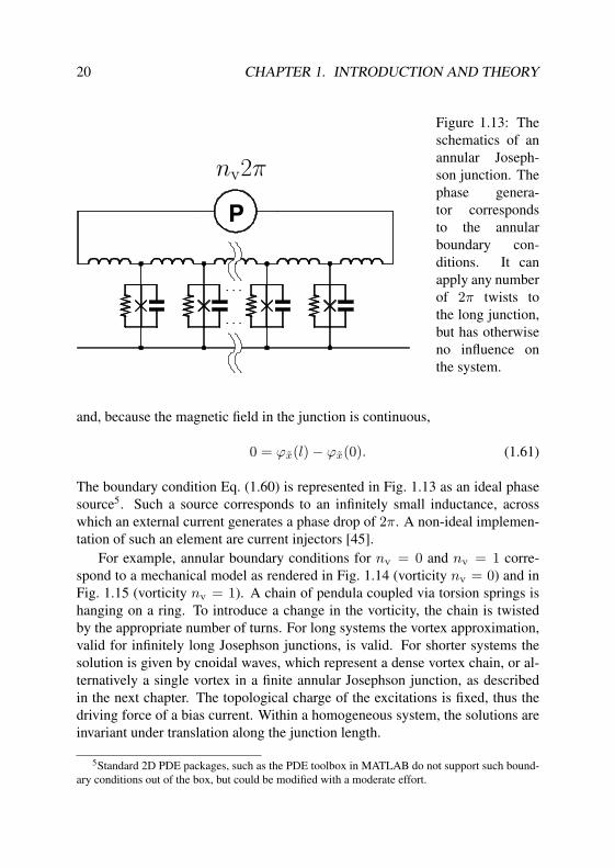
Figure 1.13: Theschematics of anannular Joseph-son junction. Thephase genera-tor correspondsto the annularboundary con-ditions. It canapply any numberof 2π twists tothe long junction,but has otherwiseno influence onthe system.
and, because the magnetic field in the junction is continuous,
0 = ϕx(l)− ϕx(0). (1.61)
The boundary condition Eq. (1.60) is represented in Fig. 1.13 as an ideal phasesource5. Such a source corresponds to an infinitely small inductance, acrosswhich an external current generates a phase drop of 2π. A non-ideal implemen-tation of such an element are current injectors [45].
For example, annular boundary conditions for nv = 0 and nv = 1 corre-spond to a mechanical model as rendered in Fig. 1.14 (vorticity nv = 0) and inFig. 1.15 (vorticity nv = 1). A chain of pendula coupled via torsion springs ishanging on a ring. To introduce a change in the vorticity, the chain is twistedby the appropriate number of turns. For long systems the vortex approximation,valid for infinitely long Josephson junctions, is valid. For shorter systems thesolution is given by cnoidal waves, which represent a dense vortex chain, or al-ternatively a single vortex in a finite annular Josephson junction, as describedin the next chapter. The topological charge of the excitations is fixed, thus thedriving force of a bias current. Within a homogeneous system, the solutions areinvariant under translation along the junction length.
5Standard 2D PDE packages, such as the PDE toolbox in MATLAB do not support such bound-ary conditions out of the box, but could be modified with a moderate effort.

1.7. ANNULAR JUNCTIONS 21
Figure 1.14: The mechanical analog of an annular Josephson junction [46] withvorticity nv = 0. The pendula (black) correspond to a section of the Josephsonjunction. The springs between the pendula are represent a torsion coupling be-tween the pendula. The situation depicted corresponds to a junction bias closeto γ = 1 under a small applied magnetic field.
Figure 1.15:The mechanicalanalog of an an-nular Josephsonjunction, vor-ticity nv = 1.The junctionlength is 20λJ
(three pendulaper Josephsonlength). Thejunction is unbi-ased and at zeromagnetic field.
22 CHAPTER 1. INTRODUCTION AND THEORY
1.7.1 Perturbation Theory: Vortex Effective PotentialsThe application of perturbation theory[47] treats statics and dynamics of LJJ vor-tex states. In this section, effective potentials for a conservative vortex equationof motion are derived. This is based on the field Hamiltonian of the system, in-cluding the bias current and the external magnetic field. The effect of dissipationis discussed in the next section.
For an annular Josephson junction, the external magnetic field term takes theform
hext(x) = hext cos(x/r), (1.62)
with r being the normalized radius of the junction, and hext the externally ap-plied magnetic field.
For annular junctions Eq. (1.44) can be rewritten as
H(ϕ, ϕt) =∫ l
0
(12ϕx
2 +12ϕt
2 − γϕ + ϕx cos(x/r)hext − cos ϕ
)dx
(1.63)The first term of Eq. (1.44) is independent on ϕ and therefore removed.
Solutions have to fulfill the boundary conditions (1.60) and (1.61). Aftersetting hext and γ to 0, the system is totally homogeneous. In the derivationof the effective potentials it is assumed that neither hext nor γ can change thesolutions of the unperturbed sine-Gordon equation, Eq. (1.37). A necessary,but not sufficient condition for this, is that for a given unperturbed solution theenergy change of the total system due to these terms is small in comparison tothe rest energy of the solution itself.
A static solution ϕf of Eq. (1.37) is generalized by Lorentz transformationto a set of solutions
ϕ(x, t) = ϕf
(x− x0 − vt√
(1− v2)
). (1.64)
In the non relativistic limit (v2 1), the only effect of the transformation is aspatial translation of the solution.
ϕ(x, v) = ϕf(x− x0 − vt). (1.65)
The time derivative ϕt is given by
ϕt(x, t) = vϕf,x(x− x0 − vt). (1.66)

1.7. ANNULAR JUNCTIONS 23
The varying terms of the Hamiltonian are given by
H(ϕ, ϕt) = lnvγ +∫ l
0
12ϕf,t
2dx︸ ︷︷ ︸12 v2m
+
∫ l
0
−γϕf,xxdx︸ ︷︷ ︸−γx0nv2π
+∫ l
0
ϕf,x cos(x/r)hextdx︸ ︷︷ ︸κf cos(x0/r)hext
(1.67)
with κf being the first Fourier component of ϕf . In general, the last term inEq. (1.67), is a convolution of the local magnetic field. For the solution definedby Eq. (1.49), corresponding to the magnetic profile
ϕf,x(x, x0) = 2sech (x− x0) , (1.68)
κf = 2πsech(π2/l
)is found [48], resulting in the potential Uh(x0)
Uh = −hext2πsech(π2/l) cos(x0/r) = −2πh cos(x0/r), (1.69)
where h = κhext.
1.7.2 Vortex DynamicsThe equation of motion for x0 is given by
mvt = 2πγ − ∂Uh
∂x0, (1.70)
where the mass m, associated with a translation of the excitation is given by
m =∫ l
0
ϕx2dx. (1.71)
For the solution given by Eq. (1.49) in an infinite junction,
m =∫ ∞
−∞ϕf,x
2(x)dx = 8. (1.72)
To take into account the effects of the dissipative quasiparticle term inEq. (1.36), the corresponding Rayleigh dissipation function[49] can be con-structed. which describes the power dissipated in the system and, therefore,

24 CHAPTER 1. INTRODUCTION AND THEORY
the change in the total energy of the modified Hamiltonian system. For the gen-eralized force, given by
γα = −αϕt, (1.73)
the Rayleigh dissipation function F is then given by
F =∫ l
0
12αϕt
2dx. (1.74)
After inserting ϕf,x, the dissipated energy is given by
F = α12v2
∫ l
0
ϕx2dx︸ ︷︷ ︸
m
. (1.75)
The vortex equation of motion Eq. (1.70) is modified to
mvt = −dUh(x0)dx0
− 2πγ − mαv. (1.76)
Any excitation residing in a small or large Josephson junction, for which thelocal expression is given by Eq. (1.19), in especial any excitation discussed inthis thesis obtains dynamical mass by the capacitive energy, which is governedby the same term as the Rayleigh dissipation function. It is therefore not a co-incidence that the mass term appears on the RHS of Eq. (1.76). The normalizeddamping η is determined by η = α, as long as the resistance Rj is the onlysource of dissipation.
The average voltage at a chosen point of the junction is proportional to thechange of the flux in the barrier. A vortex with the limiting Swihart velocity c ofelectromagnetic waves in the junction generates voltage V0, given by
V0 =cΦ0
2πr(1.77)
The specific shape of the current-voltage characteristics is determined by per-turbation theory developed by McLaughlin and Scott [47]. Perturbation theoryresults and experiments are compared in detail in Ref. [50]. In the relativisticlimit, the friction force is related to the equilibrium velocity v∞ by
F = 8v∞√
1− v∞2
(α +
β
2− (1− v∞2)
), (1.78)

1.7. ANNULAR JUNCTIONS 25
where β is the surface impedance damping parameter. Since bias current γ ex-erts a force of 2π on the vortex, Eq. (1.78) defines the current-voltage charac-teristics of a long junction. An example current-voltage characteristic for vor-ticity nv = 1 is plotted in Fig. 1.16. Residual pinning due to nearby trappedAbrikosov vortices causes a finite zero-voltage current. For a perfectly homoge-neous annular Josephson junction a zero depinning current is expected. Voltagecorresponding to the Swihart velocity c is only a fraction of the gap voltageof the superconductor. Inhomogeneities in the system cause the vortex to emitelectromagnetic waves, which cause the system to generate additional vortex-antivortex pairs. In this limit the single vortex approximation is not suitable anymore.

26 CHAPTER 1. INTRODUCTION AND THEORY
−50 0 50−8
−6
−4
−2
0
2
4
6
8
(2)
(1)
U [µV]
I [m
A]
Sample: AJJ-INJ
Figure 1.16: Acurrent-voltagecharacteristic fora vortex trappedin an annularJosephson junc-tion. At point(1) the vortexis depinned, atpoint (2) thevortex solutionbecomes unstableand the wholejunction switchesto the resistivestate. The dashedline shows a fitof Eq. (1.78) tothe experimentaldataset. The ver-tical dotted linesshow the voltagecorrespondingto the Swihartvelocity.

Chapter 2
Experimental Technique anddata evaluation
2.1 Measurement Scheme
The most typical electric measurement scheme schematized in Fig. 2.1. Thecircuit consists of a voltage-controlled current source, and a low-noise pream-plifier (high dc impedance), which together form a four wire measurement. Atthe maximum sensitivity of the setup, differential resistances on the order of mΩcan be determined without lock-in techniques. Details on the filtering circuitsand electronic error estimates are described in appendix A.
For measurements of the current voltage characteristics, the voltage outputand current monitor signals are measured by an AD converter and the controlvoltage for the current source is generated by a DA converter. Both are locatedon a buffered synchronous data acquisition card[51, 52, 53] in the controllingcomputer. Time-series of both current and voltage are measured and evaluatedby software. This allows the definition of complex waveforms, which can beused to test state preparation and readout schemes.
An alternative mode of operation of the setup allows for the control voltageto be generated by an analog function generator. The voltage signal is comparedto a threshold value, chosen to detect the transition of the system from the super-conducting (zero-voltage) state to the running (finite voltage) state by triggers.The time delay between the trigger edges of the current and the voltage trigger isacquired by a high-precision time interval counter [54]. A detailed description of
27

28CHAPTER 2. EXPERIMENTAL TECHNIQUE AND DATA EVALUATION
Voltage Amplifier
Current source
Super
con
duct
ing p
art
(2)
(1)
(4)
(3)
Figure 2.1: Sim-plified electricalmeasurementscheme. A fourwire measure-ment where thevoltage (1,2)and current (3,4)leads are con-nected at thesuperconductingelectrode. Filtersin the leads areleft out for clar-ity, for details seeappendix A .
the predecessor setup (Ref. [55]) and appendix B describe the noise properties ofthe room-temperature data acquisition equipment, while appendix A describesthe Johnson noise in the biasing resistors.
2.2 Vortex InjectionVortices in annular Josephson junctions may be trapped during the transitionof the superconducting electrodes through the critical temperature. Another,more controllable and reversible way of introducing the vortices into an annularjunction is to use a pair of current injectors which form a local current dipole[45, 56].
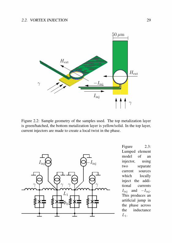
The geometry of the annular Josephson with injectors is illustrated inFig. 2.2. The corresponding lumped element model1 is schematized in Fig. 2.3.In addition to the current source homogeneously biasing the Josephson junction,two local current sources inject positive and negative current of the same ampli-tude to two neighboring nodes. According to the lumped element model, thiscell can be biased to contain an additional quantum of magnetic flux. This cor-
1This scheme represents the situation used in our experiments presented in this chapter. Insteadof an isolated current source [45], two current sources of opposite polarity are utilized. From theviewpoint of electronics, this offers significant advantages, see appendix B for a detailed explanation.
2.2. VORTEX INJECTION 29
γ
−Iinj
Hext
Hext
γ
Iinj
50 µm
Figure 2.2: Sample geometry of the samples used. The top metalization layeris green/hatched, the bottom metalization layer is yellow/solid. In the top layer,current injectors are made to create a local twist in the phase.
Φ0
L1
Iinj
γ
−Iinj
γ γ γ
Figure 2.3:Lumped elementmodel of aninjector, usingtwo separatecurrent sourceswhich locallyinject the addi-tional currentsIinj and −Iinj.This produces anartificial jump inthe phase acrossthe inductanceL1.

30CHAPTER 2. EXPERIMENTAL TECHNIQUE AND DATA EVALUATION
−50 0 50−8
−6
−4
−2
0
2
4
6
8
U [µV]
I [m
A]
Sample: AJJ-INJ
Figure 2.4:Current-voltagecharacteristicsof an injectedvortex (red,solidline) and a vortextrapped duringcooldown (black,dashed line).The subgap volt-age varied dueto unintendedtemperaturefluctuations.
responds to a phase jump of 2π over the element L1 in Fig. 2.3. Since the totalvorticity of the junction is conserved, the the phase difference of−2π distributesalong the rest of the junction. This corresponds to the phase drop induced bythe annular boundary conditions. A formed vortex can move freely along theJosephson junction. Thus, by injecting an appropriate current, the vorticity ofthe annular Josephson junction state can be changed without leaving the super-conducting state. If the distance between the injectors is on the order of a λJ orless, the net current flowing perpendicular through the junction is negligible.
The statics and dynamics of injected vortices are very similar to that of vor-tices trapped during cooldown. A comparison of the current-voltage character-istics of both is displayed in Fig. 2.4. In the zero voltage state additional pin-ning at the locations of the injectors is observed. Figure 2.5 compares the two-dimensional IC(H) patterns[10] for both types of vortices, acquired on sampleAJJ-INJ (see appendix C). Since the injected current generates magnetic flux inthe junction barrier, an additional pinning occurs at the injectors.

2.2. VORTEX INJECTION 31
−1.5 −1 −0.5 0 0.5 1 1.5−1.5
−1
−0.5
0
0.5
1
1.5
Hx [G]
Hy [G
]
(1)
(2)
(3)
I c [mA
]
0
1
2
3
4
5
6
7
8
Sample: AJJ-INJ
Figure 2.5: Comparison of the depinning current of a vortex trapped duringcooldown (dashed white lines) and an artificially inserted one (density plot,black contour). Current difference between isolines is 0.5 mA. At location (1)the patterns deviate due to parasitic pinning by the magnetic flux by the barrierat the injectors, while at (2) and (3) the critical currents coincide.

32CHAPTER 2. EXPERIMENTAL TECHNIQUE AND DATA EVALUATION
2.3 Escape Field DistributionsUnder applied bias current the zero voltage state of a Josephson junction is ametastable state. To examine fluctuations of the escape current due to thermalexcitations or quantum mechanical effects, we use the well known[3, 4, 5] tech-nique of repeatedly ramping the bias field with an analog function generator.A common model for the activation is the depinning of a point-like particle ofmass meff from a potential well, depicted in Fig. 2.6. It is convenient to definethe reduced bias field ε = (1 − γ/γcr). Thermal or quantum fluctuations causethe lifetime, defined as the inverse of the escape rate Γesc, of the trapped state tobe finite. For a wide class of potentials, both the thermal and quantum escaperates are modelled as a function of ε by the general form
Γesc(ε) = Aεa+b−1 exp(−Bεb). (2.1)
The type of activation and the damping limit of the system determines a and b,while andA and B depend on sample parameters, temperature and external fieldor current biases. In the case of thermal activation B is the ratio of the unbiasedbarrier height, and the thermal energy
B =U
kBT, (2.2)
and b = 3/2. The meaning of A and a is specific to the different dampingregimes, as discussed in the next section. In the experiments the bias current γis increased at the constant normalized ramp rate γt
γ = γtt. (2.3)
The normalized ramp rate is related to the derivative of the bias current Ib as
γt =Ib
IC
1ωP
, (2.4)
where IC and ωP are not necessarily known to a high precision. Ideally both aredetermined using spectroscopy. Otherwise both are estimated by a measurementof the critical current (density) and an estimation of the junction capacitance.The values for γt are in our setup typically on the order of 10−10 · · · 10−7. Dueto this slow ramp the system remains in equilibrium, as opposed to the inten-tional excitation technique used by Silvestrini et al. [57]. Here Γesc(t) is definedby Eq. (2.1) or more generally as a function of γ(t) only.

2.3. ESCAPE FIELD DISTRIBUTIONS 33
0 0.5−3.5
−3
−2.5
−2
−1.5
−1
−0.5
0
0.5
1
1.5
ǫ = 0.0
ǫ = 0.5
ǫ = 1.0
U/h
q
ω0
ωB
U0
Figure 2.6: Potentials depending on reaction coordinate q (curves are offset forvisibility), for different reduced bias fields ε. The dot denotes the stable mini-mum position. If ε reaches zero, the potential has no stable position any more.In a stable minimum, the particle oscillates with the small oscillation frequencyω0. For the unbiased potential, the potential barrier height U0 is indicated.
34CHAPTER 2. EXPERIMENTAL TECHNIQUE AND DATA EVALUATION
When the system is activated, the junction switches to the voltage state. Thetime interval between the moment of the bias current Ib to be zero and of thistransition to the voltage state is recorded and the bias current is set to zero.The ensemble of these time intervals forms the observations of a decay from anoccupation probability P = 1 for zero time (all members of the ensemble inzero voltage state), which decays to zero close to the critical current2.
Solving the differential equation
P = −PΓesc(γ(t)), (2.5)
with the initial value P (0) = 1, yields the cumulative distribution function(CDF). The probability distribution function (PDF) is then given by −P . In thisthesis the specific solution of Eq. (2.5) for a thermal escape is referred to as theKurkijarvi-Fulton-Dunkelberger (KFD) [3, 4] distribution. Dividing Eq. (2.5)by −P and substituting P by 1−
∫ t
τ=0P (τ)
Γesc(γ(t)) =P (t)(
1−∫ t
τ=0P (τ)dτ
) (2.6)
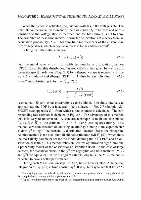
is obtained. Experimental observations can be binned into finite intervals toapproximate the PDF by a histogram like displayed in Fig. 2.7 (Sample AJJ-SHORT (see appendix C)), from which a rate estimate is calculated. The cor-responding rate estimate is depicted in Fig. 2.8. The advantage of this methodthat it is easy to understand. A standard technique is to fit the rate modelΓesc(a, b,A,B) to the estimate [3, 5, 6, 8] using least-squares fitting. Thismethod leaves the freedom of choosing an arbitrary binning to the experimenteras does χ2 fitting of the probability distribution function [58] to the histogram.Another method is the maximum likelihood estimation (MLE) [59], which findsthe most likely parameter set for the model defining the KFD PDF and an ob-servation ensemble. This method relies on iterative optimization algorithms anda probability model of the observations distribution itself. In the case of largedatasets, the statistical errors in the χ2 are negligible and both methods (MLEand χ2) are equivalent. If the histogram exhibits long tails, the MLE method isexpected to have a better performance.
During each MLE iteration step, Eq. (2.5) has to be integrated. A numericalintegration of Eq. (2.5) is time consuming3. It is quite easy to see that Eq. (2.5)
2For very high ramp rates the decay takes place (in a classical picture) after crossing the criticalforce, equivalent to having a finite population at ε = 0.
3Typical iteration counts are on the order of 100. Integration using an adaptive Runge-Kutta ODE
2.3. ESCAPE FIELD DISTRIBUTIONS 35
14.9 14.95 15 15.05 15.1 15.150
0.01
0.02
0.03
0.04
0.05
0.06
0.07
0.08
0.09
0.1
Ic[µA]
Pro
babi
lity
/ Bin
50mK300mK
Sample: AJJ-SHORT
Figure 2.7: His-tograms (1200samples) fortwo differenttemperatures.At the highertemperature thehistograms iswider due to thelower Arrheniusexponent.
is a homogeneous differential equation, where the solution takes the simple form
P (t) = 1− exp (s) . (2.7)
The persistence probability exponent s is given by
s(t) = −∫ t
0
Γescdt. (2.8)
For rates of the form of Eq. (2.1) the persistence probability s can be devel-oped into a series4 if the PDF is negligible small everywhere besides ε 1.Using s, the PDF and CDF (Cumulative distribution function) can be derived asclosed form expressions, which are suitable for MLE fitting. The series devel-oped for by Garg [60] is the following:
s(ε) =A|γt|
γcrεa χB
Bb
(1 +
a
bχ +
a(a− b)b2B2
χ2 + O(χ3))
, (2.9)
solver to an acceptable precision requires on the order of several MegaFlops per solution, while themethod used here needs roughly 100 Flops per observation and iteration.
4By partial integration.

36CHAPTER 2. EXPERIMENTAL TECHNIQUE AND DATA EVALUATION
14.9 14.95 15 15.05 15.1 15.15
103
104
105
I [µA]
Esc
ape
Rat
e / H
z
50mK300mK
Sample: AJJ-SHORT
Figure 2.8: Ratesextracted fromthe histogramsshown in Fig. 2.7.In the rate pic-ture, the Arrhe-nius exponent Bdetermines theslope.
where χ = exp(ε−b). In our experiments B 1 always holds. The physicalmeaning of this is that an unbiased or moderately biased system is not activatedwith any measurable rate. Using terms up to the first order in χ in Eq. (2.9), themean value of the reduced bias field at which the system switches is given by
〈ε〉b =B
B, (2.10)
with B given by
B = log(
γcr
γt
A 1bB(1+a/b)
). (2.11)
At the mean escape current, B1/b is the exponent in Γesc. The standard deviationis given by
σ2 =16
(B(−2+ 2
b )
B2/bb2
). (2.12)

2.4. THERMAL ESCAPE IN A WASHBOARD POTENTIAL 37
2.4 Thermal Escape in a Washboard PotentialIn the following all escapes are treated for a one dimensional washboard poten-tial. A washboard potential is an effective potential expressed as a function of ageneralized coordinate q in the form
U = −U cos(q
r
)− γq, (2.13)
where U is the potential barrier height at zero bias current, and r sets the lengthscale of the potential well. In our systems r is either the normalized radius ofan annular junction, or r equal to one in the case of a small junction. In thispotential, a metastable state exists as long as the condition γ < γcr remainsfulfilled, with γcr given by
γcr = U 1r. (2.14)
After determining the equilibrium position, the potential barrier at a given biascurrent is calculated to be
U0 = U
√1−
(γ
γcr
)2
. (2.15)
A cubic approximation (O(3) in q) of U0 around γ = γcr, i.e. ε = 0, yields
U0 = Uε3/2 (2.16)
where U = U√
22/3. The coefficient is due to the cubic approximation of thecosinusoidal potential. The equation of motion with friction is given by
qtt =Uq − γ
meff− ηqt, (2.17)
where meff is the effective mass associated with q. This equation of motion leadsto a small oscillation frequency ω0 in the metastable state
ω0 = Ω0
(1−
(γ
γcr
)2)1/4
, (2.18)
where Ω0 is given by
Ω0 =1r
√U
meff. (2.19)

38CHAPTER 2. EXPERIMENTAL TECHNIQUE AND DATA EVALUATION
Eq. (2.18) can be developed to the first order around ε = 0:
ω0 = Ω0ε1/4. (2.20)
Classical and quantum escape dynamics are, for a single event, modelled[61] using the variable parameters ω0 and U0, and the constant temperature T ,damping η and mass meff . Thermal fluctuations cause an escape rate from ametastable well which depends exponentially on the negative inverse of the tem-perature T . This is due to the probability of finding an instance of the thermalensemble at the barrier energy. Thus,
Γesc = A exp(− U0
kBT
)= A exp
(− U
kBTε3/2
)= A exp
(−Bε
3/2)
, (2.21)
where A is the Arrhenius factor of the system, which depends on damping, asdiscussed below. Physically B = U/kBT corresponds to the Arrhenius exponentof the unbiased system, and the exponent for use in Eq. (2.1) b = 3/2.
2.5 Damping RegimesThere are different damping limits, as realized already by Kramers.
1. The simple transition state theory (TST) neglects damping and assumes athermalized occupation of phase space. In this case a particle on a givenphase space trajectory arrives one time per small oscillation at its highestpotential energy. A phase space diagram without damping is plotted inFig. 2.10a. If the thermal energy exceeds the barrier height, the particleescapes from the well. In this case the prefactor A in Eq. (2.21) is givenby the attempt frequency (the small oscillation frequency)
A =ω0
(2π), (2.22)
equivalent to (see Eq. (2.20)):
A =Ω0
2πε1/4 = Aε
1/4, (2.23)
with A = Ω0/2π and a = −1/4.
2. The low damping limit is very similar to the first case discussed above,but it is necessary to reconsider the condition of thermal equilibrium of

2.5. DAMPING REGIMES 39
the ensemble. For low damping, the system is nearly Hamiltonian. Ther-malization happens by a fluctuating force, which in electrical circuits oc-curs due to the Johnson noise (see Eq. (1.20)), existent according to thedissipation-fluctuation theorem. In the limit of high resistance (low damp-ing) the escape is limited by the transport in the energy direction, becauseduring a single small oscillation period the noise current does not redis-tribute the particle state in the well, but only causes a slow diffusion in theenergy direction. This was already recognized by Kramers [61]. For thevery low damping limit ηU0/kBT 1
A =185π
ηBε3/2, (2.24)
resulting in A = 185π ηB and a = 1.
3. In the strong damping limit, the momentum of the particle, needed to over-come the barrier, is larger because of the friction. For the same startingpoints as in Fig. 2.10a, Fig. 2.10b shows the strong damping case. Theexpected flux over the barrier (integrating over all trajectories from thesaddle point to infinite momentum, weighted by the thermal ensemble)is reduced by the damping. This case is not relevant for the experimentsdescribed in this thesis.
These three cases correspond to a transport in the phase space limited in differentways. In the moderate damping regime, the limit the transport of an ensembleof along the bound phase space trajectories - the noise is strong enough to redis-tribute the particles after some oscillations. In the low damping limit, the noisecan not redistribute an ensemble across all bound states after a small number ofoscillations. The coefficients for the different cases are listed in Table 2.1.
Calculating the PDF for the corresponding cases shows that for typical pa-rameters in our experiments, only the weak damping limit imposes a severechange on the distribution, compared to the TST case. For the same value ofU , with a ramp rate of γt = 10−11, Fig. 2.9 shows the calculated distributions.Relevant to the experiments presented here are the weak and the moderate (TST)damping regimes. These cases are bridged in Ref. [62]. The TST expressionholds for a moderate damping, but a constant correction to the escape rate hasto be carried out. According to Ref. [62], the correction to the TST rate (A) isgiven by
Γesc
Γesc(TST )=√
1 + 4αΥ−1 − 1√1 + 4αΥ−1 + 1
Υ, (2.25)
40CHAPTER 2. EXPERIMENTAL TECHNIQUE AND DATA EVALUATION
Mechanism Damping A B a b
Thermal Low 18η5π Bth Bth 1 3/2
Thermal Moderate Ω02π Bth −1/4 3/2
Thermal High Ω02
2πη Bth 0 3/2
Quantum None(
30Bquπ
)1/2
Ω0 Bqu 5/8 5/4
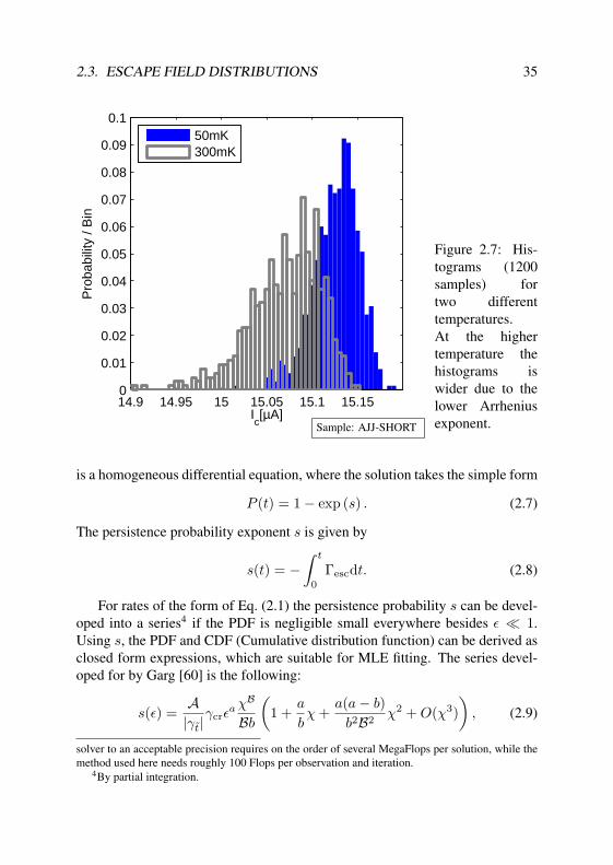
Table 2.1: Coefficients (table taken from Ref. [60]) for the three damping limitsfor thermal activation and the quantum limit. In the thermal limit, the threedifferent regimes correspond to the following situations: Escape rate over thebarrier depletes the phase space, because the coupling to the bath does nowallow for a thermalization (low damping). System thermalizes on the order ofthe expected lifetime of the metastable state (moderate damping). The dampinghinders the system to escape over the barrier (high damping). In the vortex case,
the Bth and Bqu are given by Bth = UkBT
= 4πh 23
√2
kBT, Bqu = 36U
5Ω0~ = 365
4π√
8h
~ .
00.0020.0040.0060.0080.01−0.01
0
0.01
0.02
0.03
0.04
0.05
0.06
0.07
ǫ
∂P
(ǫ)/
∂ǫ
TSTη=1e−07η=1
Figure 2.9:Comparison ofthree differentswitching cur-rent distributionsfor the samepotential, thesame ramp rateof γt = 10−11,but two differentvalues of thedamping η andfor the TST re-sult, respectively.

2.6. PARAMETER ESTIMATION 41
where α is a constant of order 1 and Υ is given by
Υ =ηSb
kBT=
3 · 25/4
10ηS0
kBTε5/4, (2.26)
where Sb is the action of the path from the top of the barrier to the bottom andback for a given value of ε. S0 is the action of this path at ε = 1. For thewashboard potential, S0 = 16
√meffU [62, Eq. 2.9].
2.6 Parameter EstimationIt is not possible to determine the a priori unknowns (η,IC,Ω0,U) as independentparameters. Ideally, γcr is determined independently from a spectroscopic mea-surement. If this is unavailable5, it is suitable (in the small JJ case) to proceedas follows:
1. Estimate Ω0 from the nominal sample parameters.
2. Perform MLE fitting of datasets from different temperatures, using A asfixed and B and γcrIC as free parameters. Take the ratio of the barrierheight B in units of the thermal energy to the Josephson energy given byEq. (1.11) for the corresponding IC. For moderate damping the BT/IC
ratio matches the TST value.
3. Fit the datasets with A as a free parameter using the assumption of a fixedBT/IC ratio. Compare to the theory by Buttiker et al.[62]. The resultof this procedure can be seen in Fig. 2.11, where the analytical line wasdrawn using Eq. (2.25), for the 1 kA sample SJJ-DAMP (see appendix C).Neglecting the strong and weak damping regimes leads to an underesti-mation of the barrier height6. It must be stressed that leaving IC and Bas free independent parameters in any TST-like fit can compensate for nottaking the change of A into account and still lead to acceptable fits, sincethe freedom to shift and scale the distribution reproduced the effect of achanged damping .
5On some of the experiments presented, the coupling between the antenna and the sample wasnot sufficiently flat.
6This leads either to an overestimation of the escape temperature, which may be an alternativeexplanation for [8, Fig. 6.28(b), Fig. 6.22], or an underestimated standard deviation, which mayinfluence the interpretation of [63, Fig. 3]

42CHAPTER 2. EXPERIMENTAL TECHNIQUE AND DATA EVALUATION
−2 0 2−3
−2
−1
0
1
2
3
Position q
Mom
entu
m p
(a) No damping (Hamiltonian) case
−2 0 2−3
−2
−1
0
1
2
3
Position qM
omen
tum
p
(b) Strong damping
Figure 2.10: Phase space of a damped particle in a cubic well. Phase space tra-jectories for both cases were integrated starting from the position at the bottomof the well (q = −1), and momenta p, which fill the well and a range of mo-menta, chosen for illustration, lying on unbound trajectories in the Hamiltoniancase (a). While in (a) all instances which lie outside the separatrix (black) lineescape over the barrier (q = 1), in (b) some of these cross the separatrix andremain within the well.
2.7 Conclusion
Two dimensional IC(Hx,Hy) patterns[10] were used to examine injected vor-tices. A comparison of the injected vortex IC(Hx,Hy) pattern to the pattern ofa vortex trapped during cool down shows the locality of the residual potentialcreated by current injector [45, 56]. This demonstrates that in extended circuits,a vortex injector does not influence the vortex behavior at distances substantiallylarger than the Josephson penetration depth λJ .
To prove the setups performance we use the well known experimental tech-nique of ramping the bias current and determine the critical current and thedamping parameter of a small Josephson junction. A turnover from the moder-ate to the weak friction regime is observed, and the dependence of the dampingon temperature agrees qualitatively with earlier observations [58], despite of adifferent data evaluation scheme, based on a direct maximum likelihood esti-

2.7. CONCLUSION 43
1 2 3 4 5 6 70
0.5
1
T[K]
I c[mA
]
10−2
10−1
100
ATST
Sample: SJJ-DAMP
Figure 2.11: Bottom: MLE fitting result using TST scaling for critical currentfor experimental data from 1 kA/cm2 SJJ of area 100 µm2. The only free param-eters where A and IC. Using Eq. (1.11), B = Φ0
2πkBT IC. The critical currentdensity using the temperature dependent superconducting gap for the calcula-tion of the critical current density using the Ambegaokar-Baratoff theory andapproximated temperature-dependence of the gap [28, 31], with a critical tem-perature of Tc = 6.6 K, which fitted for unknown reasons the experimental data.Top: The prefactor A represents the normalized plasma frequency ωP , modifiedby weak-to-moderate damping. The solid line represents the scaling of A, ac-cording to Eq. (2.25) (evaluated at the average value of ε) and Eq. (1.15), wherethe resistance was put to be approximately 102 times smaller than the value ex-pected from the normal resistance (compares well to Ref. [58]). The data pointsat the highest temperatures were subjected to a fluctuation of the temperature,and not taken into account.

44CHAPTER 2. EXPERIMENTAL TECHNIQUE AND DATA EVALUATION
mation of escape events. We observe a shunting resistance to be significantlysmaller than the predicted quasiparticle resistance. This is most likely due to theinfluence of the finite impedance of the electromagnetic environment [64].

Chapter 3
Metastable Vortex States
States of vorticity nv = 1 with a single flux quantum trapped between the su-perconducting rings of an annular Josephson junctions were first investigatedexperimentally in Ref. [65]. The experimental results presented in this chap-ter where achieved during the investigation of the escape of vortices from ametastable state formed by magnetic field and bias current. For this, ramp-typeensemble measurements are used, in the same way as in [9, 8] and described inthe previous chapter. The predicted scaling of the small oscillation frequencywith magnetic field and bias current is verified by resonant spectroscopy. In thischapter, spectroscopic measurements on intermediate length (l ≈ 10λJ ) andthermal activation measurements on short (l ≈ 4λJ ) junctions are presented.Both junctions are µm-scaled and were produced using photo-lithography at acommercial foundry[66]. The question of how far the elementary excitations inthis finite systems coincide with soliton excitations in infinite junctions is treatedin terms of a harmonic model, which coincides for short junction lengths withthe cnoidal wave solution, (see e.g. [67, 68, 69]).
3.1 Metastable Vortex States
A single, resting Josephson vortex can undergo a transition from a static, pinnedstate (zero-voltage) to a dynamic, moving state (finite voltage). This process isequivalent to the activation of a small junction, but the activated variable is notthe phase difference, but the center of mass position of a vortex .
The fluctuation-free depinning current γcr, is found by equating the magnetic
45

46 CHAPTER 3. METASTABLE VORTEX STATES
field force Fh maximum
Fh = −2πh
rsin(x0/r) (3.1)
to the bias current driving force 2πγcr. In the fluctuation free case the metastablestate vanishes at
γcr =h
r, (3.2)
and the system switches to the voltage state as discussed in sec. 1.7.2. In thepresence of finite temperature or quantum fluctuations, the escape happens froma metastable state, as depicted in Fig. 2.6, with the vortex coordinate x as the dy-namic variable. In addition to the minimum x0 a potential maximum at positionx1 exists as a metastable equilibrium point. The positions of these are given by
x0,1 = r
(π ± π
2∓ arcsin
(γr
h
)). (3.3)
The minima for different bias currents are marked in Fig. 2.6 by a dot.In the region of validity of the vortex perturbation theory, the critical current
is linear in the magnetic field. In order to describe the dynamics of the systemin the presence of fluctuations, the barrier height U0 and the small oscillationfrequency in the well ω0, indicated in Fig. 2.6, suffice to describe the dynamicsof the system. Evaluating the potential at the positions calculated in Eq. (3.3)results in the barrier height
U0 = 4πh︸︷︷︸U
√1−
(γ
γcr
)2
. (3.4)
The small oscillation frequency (in normalized units), is given by
ω0 = 2π1r
√h
m︸ ︷︷ ︸Ω0(h)
4
√1−
(γ
γcr
)2
. (3.5)
This relation is verified by resonant spectroscopy in the next section, where foreach given magnetic field, N measurements (ω0iωP , γiIC), i = 1..N form theset of observed values 1 with a model parameter vector (Ω0ωP , ICγcr). The
1Independent variable: ω0iωP , dependent variable: γiIC. In real experiments in the next sectionthere exists the power of the resonant probing as a hidden variable, which is not modelled.

3.2. SPECTROSCOPY ON AN ANNULAR JUNCTION 47
scaling of Ω0ωP is predicted to be proportional to (ICγcr)1/2, explicitly:
Ω0ωP
(ICγcr)1/2=
ωP√IC
Ω0√γcr
(3.6)
This is expressed in physical units as
Ω0ωP
(ICγcr)1/2=
√1
2πwr
√2π
Φ0C∗j
√1
lmeff(3.7)
Thus, without knowing h, a self-consistent analysis can be carried out. It isinstructive to more closely analyze what parts of Eq. (3.6) contribute in whichway. The first term,
ωP√IC
=
√2π
Φ0C∗j
√1
2πwr, (3.8)
is related to the capacitive charging energy only, while the second term,
Ω0√γcr
=√
1lmeff
∝ jc−1/4, (3.9)
is related to the rest mass of the solution. It might seem counterintuitive thatthe critical current density jc of the Josephson junction enters as a power of1/4. This is understood when taking into account that a change of the Josephsonlength causes the vortex solution to change its scale. This is different to the caseof a small Josephson junction, in which the relationship Ω0 ∝ jc
1/2 is observed.
3.2 Spectroscopy on an Annular JunctionThe dependence of ω0 on the bias current can be verified by adding an rf biasto the dc bias and observing the rate of decay as a function of the bias current,a technique applied earlier to small junctions [70], and to vortices in narrowJosephson junctions [9]. In the classical interpretation, small oscillations of thevortex position are excited [71, 72]. The amplitude of these depends on thedetuning of the rf from the small oscillation frequency of the system, and theapplied power. At a single value of ε, the small oscillation frequency correspondsto the externally applied frequency ν
ν = ω0/2πε1/4 (3.10)

48 CHAPTER 3. METASTABLE VORTEX STATES
00.050.10
5
10
15
20
25
Cou
nts
ǫ
resonant
thermal fluctuation
Sample: AJJ-MS2
Figure 3.1: Asingle histogramin the presenceof an rf drive(13 GHz). Non-resonant escapeoccurs at reducedbias fields ε closeto zero with theaid of thermalfluctuations.Resonant escapetakes place at alarger value of ε.
and the oscillation amplitude reaches its maximum.For frequencies small in comparison to Ω0, a rate enhancement is observed,
given by the ratio of the decay rate with rf bias to the decay rate of the dc onlybiased system. A Lorentzian peak in the rate enhancement (Γesc,rf−Γesc)/Γesc,where Γesc is the decay rate without rf bias and Γesc,rf is the decay rate with rfbias, is expected to be centered around the resonant frequency. In the measure-ments presented next, high frequencies were used. In this case the resonant peakis clearly separated from the ground state peak, as shown in Fig. 3.1, acquired onsample AJJ-MS2 (see appendix C). In this limit a double peak in the switchingcurrent distribution is observed. Although the theoretical criterion for selectingthe rf amplitude is arbitrary, the automated data acquisition software used for themeasurments presented in this chapter chooses the power such that both peakshave approximately the same probability.
A typical resonance curve of the depinning process in the annular junctionAJJ-MS2 (see appendix C)can be seen in Fig. 3.2. When changing the frequencythe position of the resonant peak shifts. The maximum of the resonant peak isdetermined; so that a relation between the bias current an the frequency can bedetermined. At this point, γcr is still unknown, as well as the unbiased small

3.2. SPECTROSCOPY ON AN ANNULAR JUNCTION 49
oscillation frequency Ω0. So it is a priori impossible to determine the value of ε.Since the relation ω0 = Ω0(1− (γ/γcr))
1/4 is a nonlinear one, γcrIC, as well asΩ0ωP can be interpreted as free fitting parameters. This fitting was carried outin Fig. 3.2 to find the most likely parameters. The resulting resonance curve isindicated by the dashed line. After the fluctuation free depinning current γcrIC
is known, it is possible to determine the corresponding values of the reduced biasfield, plotted on the y-axis in Fig. 3.2. In Fig. 3.2, there are some systematic de-viations, and some random outliers. In order to understand these, it must be keptin mind that the rf amplitude varies strongly with frequency. A clear distinctionmust be made: the rf amplitude varies due to the electric environment of thesystem, and the rf amplitude required for the vortex escape from the metastablestate also varies. The latter depends on the height of the barrier to be surpassed,and thus on the frequency. In Fig. 3.2, the effects of both power variations areevident. Around 13 GHz, the coupling to the junction of the generator variedstrongly. Another pronounced structure is the transition at 10 GHz. This maybe attributed to a effect of the finite temperature at 150 mK. The crossover tem-perature [73] T ∗ = ~ν/kBT is calculated to be 72 mK. Whether the step in themean switching current is step is bound up with T ∗ could be verified by mea-surements at different temperatures. The mechanism by which such a step couldbe explained is that the escape from the resonant peak is supported by thermalfluctuations down to the crossover temperature, lowering the required power,while below the crossover temperature, thermal activation is suppressed, so therf amplitude must be increased in order to drive the vortex resonantly over thebarrier. But at small values of the reduced bias field, the frequency, and thereforethe crossover temperature drops to zero. Hence non-resonant activation dependson the rf signal and the thermal noise.
When repeating the procedure several times at different magnetic fields, therelation Eq. (3.6) between the depinning current and the small oscillation fre-quency at zero bias is found experimentally. In this experiment three differentmagnetic field amplitudes and three angles of magnetic field are chosen. Foreach a series of histograms exhibiting a double peak was acquired for differentfrequencies. By fitting to this data the fluctuation free depinning current γcrIC
and the unbiased small oscillation frequency are determined. In Fig. 3.3 the re-sult of this procedure is compared to the theoretical prediction. The slope of theindicated line was chosen to fit the data.

50 CHAPTER 3. METASTABLE VORTEX STATES
8 10 12 140
0.05
0.1
0.15
ν [GHz]
ǫ
Sample: AJJ-MS2
Figure 3.2:Switching currentprobability as afunction of thebias current. Thesmall oscillationfrequency rela-tion ν(γ, h) =ε1/4ν(γ = 0, h)is fitted to themedian currentof the resonantpeak. Thishistogram wasacquired at atemperature of150 mK. Themain peak isnon-resonantlyshifted by the rfcurrent.
3.3 On Classical Resonances and Quantum Tran-sitions
The number of levels in a well is determined by ε, which in turn is determined bythe resonant frequency νtrans. In a well of potential depth U and small oscillationfrequency ω0 we find approximately n quantum levels
n =U0
~ω0
, (3.11)
assuming the dynamics of a harmonic oscillator. Rewriting in terms of the re-duced bias field, and the potential height U and small oscillation frequency Ω0
at zero bias yields
n =Uε3/2
~Ω0ε1/4
=U
~Ω0
ε5/4. (3.12)

3.3. ON CLASSICAL RESONANCES AND QUANTUM TRANSITIONS 51
0 0.01 0.02 0.03 0.040
5
10
15
20
25
30
35
Ic1/2(A1/2)
ν 0(GH
z)
90o
180o
270o
Theory
Sample: AJJ-MS2
Figure 3.3: Several measurements on sample AJJ-MS2 (see appendix C), at dif-ferent angles of the applied magnetic field for three different magnetic field am-plitudes. The two independent fitting parameters, obtained from measurmentsas presented in Fig. 3.2, are plotted. The expected dependence, estimated fromspecific capacitance (chosen to match the threshold voltage of a vortex step), andcritical current density (approximated by the maximum switching current in theabsence of field at nv = 0), is indicated by the dashed line.
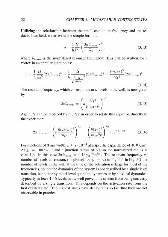
52 CHAPTER 3. METASTABLE VORTEX STATES
Utilizing the relationship between the small oscillation frequency and the re-duced bias field, we arrive at the simple formula
n =1~UΩ0
(2πνtrans
Ω0
)5
, (3.13)
where νtrans is the normalized resonant frequency. This can be written for avortex in an annular junction as:
n =1~U
Ω06 (2πνtrans)5 =
1~
U√U
meffr
6 (2πνtrans)5 =(meffr)3
~U2(2πνtrans)5
(3.14)The resonant frequency, which corresponds to n levels in the well, is now givenby
2πνtrans =
(n
~U2
(meffr)3
)1/5
(3.15)
Again, U can be replaced by γcrr2π in order to relate this equation directly tothe experiment.
2πνtrans =
(n
~(2πγcr)2
meff3r
)1/5
=
(~(2π)2
meff3r
)1/5
γcr2/5n
1/5 (3.16)
For junctions of 3 µm width, ~ ≈ 7 · 10−4 at a specific capacitance of 40 fF/µm2.At jc = 100 A/cm2 and a junction radius of 50 µm the normalized radius isr = 1.3. In this case 2πνtrans = 0.13γcr
2/5n1/5. The resonant frequency vsnumber of levels at resonance is plotted for γcr = 2/3 in Fig. 3.4 In Fig. 3.2 thenumber of levels in the well at the time of the activation is large for most of thefrequencies, so that the dynamics of the system is not described by a single leveltransition, but either by multi-level quantum dynamics or by classical dynamics.Typically, at least 4−5 levels in the well prevent the system from being correctlydescribed by a single transition. This depends on the activation rate from thefirst excited state. The highest states have decay rates so fast that they are notobservable in practice.
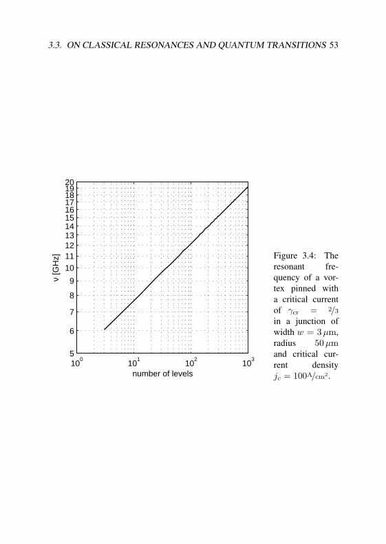
3.3. ON CLASSICAL RESONANCES AND QUANTUM TRANSITIONS 53
100
101
102
103
5
6
7
8
9
1011121314151617181920
ν [G
Hz]
number of levels
Figure 3.4: Theresonant fre-quency of a vor-tex pinned witha critical currentof γcr = 2/3
in a junction ofwidth w = 3 µm,radius 50 µmand critical cur-rent densityjc = 100A/cm2.

54 CHAPTER 3. METASTABLE VORTEX STATES
3.4 Thermal Activation of a VortexWhen varying the external magnetic field strength, the effective potential bar-rier height for a vortex is changed. This means that it is possible to change theArrhenius factor B without changing the temperature. So it is possible to inde-pendently examine the influence of both quantities on the standard deviation.
The standard deviation of the critical force of a depinning process from abiased washboard potential, as discussed in sec. 2.3, is given by
σ2 =16
(B(−2+ 2
b )
B2/bb2
). (3.17)
While the specific role of B depends on the damping, to be discussed below, band B have the same meaning for all thermal activation process, namely B =2U/kBT , and b = 2/3 being the exponent of the potential ε for ε 1. Thecubic approximation sets U = 2/3
√2U , where U is the unbiased potential barrier
height. Explicitly, this means that unless B depends significantly on B, a simplepower law scaling holds between the standard deviation of the reduced bias fieldat the time of activation and the potential height. The magnetic field generatedpotential Uh in a long Josephson junction is given by
Uh = 2πh, (3.18)
which can be written as a function of the junction radius
Uh = 2πγcrr. (3.19)
The Arrhenius factor B is then given by
B = γcr
4/3π√
2r
kBT. (3.20)
If the reduced bias field ε is small, the mean value of the switching currentsin a single histogram is a good approximation for γcrIC. If the normalizedBoltzmann constant kB, the normalized junction radius r, and B are known,it is possible, without any further information, to compare the expected stan-dard switching current distribution width to the experiment. The quantities rand kB can be estimated from the critical current density jc of the junction. Fig-ure 3.5 contains such a comparison. For arbitrary values of B the scaling ofthe switching current distribution width is indicated by a dashed lines. The ex-perimental data, consisting of datasets containing 1200 switching events, was

3.4. THERMAL ACTIVATION OF A VORTEX 55
acquired on an annular junction of width w = 2µm, radius 50 µm, and criticalcurrent density 25 A/cm2 at temperatures from 300 mK to 3.5 K. The values ofB are indicated on the dashed line. Before the different regimes are discussed,it is necessary to consider the dependence of σ on B. The factor of 5 betweenB = 2 and B = 10 corresponds to approximately the same factor in σ as to tothe 1000-fold increase between B = 10 and B = 10000. For thermal activation,σ scales as σ ∝ B−1/2. This means that for large arguments of the logarithmin Eq. (2.11), the specific value of B cannot be determined by such a technique,since it becomes exponentially imprecise. The numeric value of B is found by
B = log(
γcr
γt
A 1bB(1+a/b)
), (3.21)
where b = 3/2 for thermal activation, γt is the normalized ramp rate, A has themeaning from table 2.1. Solving Eq. (3.20) for γcr yields
γcr = B kBT
4/3√
2πr. (3.22)
Hence, Eq. (3.21) can also be written as
B = log
(kBT
4/3π√
2rγt
A 1bB(a/b)
). (3.23)
It is now obvious that B changes with B, but this change is normally small inhigh temperature limit.
The prefactorA is listed from the different cases in Table 2.1, which is takenfrom [60]. Using the prefactor for the moderate damping, B is determined to beB = log(2.8 · 10−6), for γt = 10−9,B = 103, r = .55 and kB = 1/800 K−1
and T = 3.5 K. This fits to Fig. 3.5. To match the low-temperature datasets, thelow-damping regime is appropriate. At a damping of η = 10−4, T = 300mKand B = 2 · 103, B = log(17). The agreement in Fig. 3.5 is acceptable, tak-ing into account that the standard deviation is systematically increased by theexperimental noise.

56 CHAPTER 3. METASTABLE VORTEX STATES
103
104
10−3
10−2
log(100000)log(1000)
log(10)
log(2)
log(1.2)
3..1.5K300mK
U0
kBT
σ(ε)
Sample: AJJ-SHORT
Figure 3.5: Logarithmic plot of the standard deviation of the reduced biasfield ε vs. B, which was estimated from the mean switching current and theestimated junction length (3.5λJ ). The datasets were obtained at differenttemperatures (3.5, 3, 2.5, 2, 1.5, .3) K. Within each dataset the potential bar-rier height was varied by varying the external magnetic field. The dashedlines indicates the scaling of the standard deviation for five values of B =(log(1.2), log(2), log(10), log(1000), log(10000)), as indicated on the line.

3.5. FROM THE LOW DAMPING REGIME TO THE QUANTUM REGIME57
3.5 From the Low Damping Regime to the Quan-tum Regime
The damping in the low temperature limit, is assumed not to be dominated bythe quasiparticle tunneling given by Eq. (1.15). In this limit, the dominatingsources of damping are the real part of the environments admittance at the smalloscillation frequency of the system [64] or the dielectric loss in the insulatinglayer of the window region. Decoherence considerations [74] and later spec-troscopic measurements were brought into agreement by Martinis et al. [75]with dielectric loss measurements by microwave absorbtion [76], where bathis formed of two-level systems (TLS) formed by defects in the dielectric. SinceTLSs can be saturated, the temperature and power dependence of this dissipationsource is nontrivial (see Figure. 1 of [76]), exhibiting a saturation. Spectroscopicmeasurements on small Josephson junctions [75], where only a few polarizableresonators reside in the junction barrier and window region can provide explicitstatistics of two level systems in the barrier. The specific method of depositionof the dielectric has significant influence of the behavior of the TLS [75, 77].In the experiments presented in this work, no system was designed for a highisolation [64] from the environment at high frequencies, needed to observe reso-nances with a low frequency splitting, so that no direct estimation of η at in thislimit is possible.
In Fig. 3.6, measurements carried out at temperatures on AJJ-SHORT (seeappendix C)between 28 mK and 302 mK are presented and compared to thelow-damping thermal escape calculations. The datasets are restricted to the lim-its of validity of the vortex approximation, see sec. 3.6. At a damping value ofη = 4 · 10−4 the predicted standard deviation at a temperature of 200 mK and302 mK matches to the experimental results. The Josephson energy is extrap-olated from the high-temperature regime. The barrier height is estimated fromthe mean switching current and the junction radius. Both are estimated from thecritical current density. The scaling for the thermal activation measurement, isindicated as solid lines for the two temperatures. What is most interesting inFig. 3.6 is that for the two datasets at a temperature of 133 mK and 28 mK thescaling (slope in the logarithmic plot) is changed in comparison to the other twodatasets. To verify that we are dealing with a crossover to the quantum regime,we examine this regime closer. The usual criterion[78, 79], in the TST regimefor the crossover is
T ∗ =~ωB
2πkB, (3.24)

58 CHAPTER 3. METASTABLE VORTEX STATES
2000 5000 10000 20000 50000 100000 200000
50
60
70
80
90
100
110
B = U0/kBT
σ(I
c)[
nA
]
302 mK
200 mK
133 mK
28 mK
Sample: AJJ-SHORT
Figure 3.6: Standard deviation of switching current vs. B (thermal) plotted onlogarithmic axes. The datasets were limited to a single magnetic field polar-ity and switching current values IC from 30 µA (standard deviation limited byelectronic noise) to 80 µA (validity of vortex approximation). Lines and sym-bols correspond to set temperatures of 28, 133, 200, 302 mK, as indicated. Solidlines indicate the low-damping limit thermal activation prediction. Dashed linesindicate the predicted ground state quantum tunneling distribution widths; tomatch the data, the latter ones are scaled by a constant.

3.5. FROM THE LOW DAMPING REGIME TO THE QUANTUM REGIME59
where ωB is the oscillation frequency in the flipped over barrier potential. In thecubic potential ωB = ω0 this condition is equivalent to the thermal energy beingsmall in comparison to the energy level spacing.
Experimentally quantum tunneling causes a saturation of the standard devia-tion of the switching current distribution for low temperatures. This is equivalentto a saturation of the mean of the switching current, thus the reduced bias fieldε. Due to 1/f noise in the electronics, the saturation of the distribution width iseasier to observe (see appendix B). As a matter of fact, both conditions are quiteeasily related by comparing Eq. (2.10) and Eq. (2.12). This yields a relationbetween 〈ε〉 and σ(ε):
σ(ε) = 〈ε〉B−1 π
b√
6(3.25)
Thus, if b ≈ 1 for all processes involved and the value of B is similar for thequantum and the thermal process activation, a larger value of σ(ε) is associatedwith a larger value of 〈ε〉. It is necessary to keep in mind that B is given byEq. (2.11), using the low-damping value for A in the thermal case, while theWKB approximation is used in the quantum case,
B = log
(γcr
γt
√30π
Ω0
Bqu
), (3.26)
where Bqu is given by
Bqu =36U5Ω0~
=365
4π√
8h
~. (3.27)
In the WKB approximation Bqu is proportional to the action of the trajectoryfrom the bottom of the well to the top of the well. In order to determine the tem-perature and magnetic field of the crossover for a given ramp rate and damping,〈ε〉 is compared for the quantum and the thermal case:
〈ε〉qu
〈ε〉th=
Bqu4/5
Bth2/3︸ ︷︷ ︸
log γcrγ
t
30π
~meff r
log γcrγ
t
18η5π
23 ( kBT
U )3/2
· Bth2/3
Bqu4/5︸ ︷︷ ︸
U2/15 ( 536 ~Ω0)
4/5
(kBT)2/3
(3.28)
The first factor diverges at very low temperatures, indicating that the thermalescape breaks down, and approximation by Garg Eq. (2.12) does not hold any

60 CHAPTER 3. METASTABLE VORTEX STATES
more. In the limit of low ramp rates and high damping the change of the loga-rithmic factor may be negligible. In our the term ηkBU/T dominates, and thelogarithm in the denominator changes rapidly. For a damping of η = 10−5 thesaturation temperature is approximately 150 mK. In Fig. 3.6 the change of thescaling takes place between 133 mK and 200 mK. The temperature calculatedabove for the crossover lies between these temperatures. The scaling of the ex-pected standard deviation, calculated using Bqu, Bqu, and ~ using Eq. (2.12) isindicated using dashed lines in Fig. 3.6. Yet the absolute standard deviation inthe quantum case is roughly 7 times lower than the observed one. There areseveral different possible explanations for that; the most simple one, which iscommonly used as an alibi for unaccounted results is to claim that the resolu-tion of the experimental setup limits the minimum distribution width acquired.Obviously, Fig. 3.6 shows the scaling for data points of all plotted standard devi-ations; the measurement noise for this ramp rate is on the order of 40 nA. Thereis the possibility of a saturation of the bath temperature (due to the changing crit-ical current and dissipated power), which would have a strong dependence on thebias current, but not on temperatures below the crossover. Yet this hypothesishas to be excluded fully in future experiments. Another, more sophisticated ex-planation is based the constant temperature of parts of the filtering system (seeappendix A for details). If a part of the Johnson (white) noise spectrum is notfiltered on the way to the junction, it biases the junction with colored, broadbandnoise. This effect can not be measured in terms of standard deviation, but wouldappear as an additional heat source to the junction. One alternative explanationcould be given by the fact that the vortex is not a localized particle, but, in ourcase distributed along the whole junction.This may be taken into account usingnonlocal models of the system [80], or by adopting to the short junction limitthe path integral approach used previously for the long junction limit [81, 82] .A simpler possible explanation is, that the experiments show quantum tunnel-ing, where not only the ground state is populated. External sources can be heldresponsible for this, e.g. the finite ramp rate, or colored noise from the biasingcircuitry. A likely reason for the discrepancy is neglecting the influence of tem-perature and damping at the time of escape. This can be explained in a handwaving approach by the fact that the standard deviation caused by the thermalfluctuations is changed. The physical reason for this is a non-thermal distributionof energies in the well in the low-damping limit. This non-thermal distributionis equivalent in the quantum limit to a non-thermal occupation probability of thestates - in a way that the upper states are populated stronger than they shouldbe. For an explanation of a possible way to go I refer the reader to section IX.D,IX.E, and Fig. 43 of reference [78] and [83].

3.6. CROSSOVER TO THE SMALL JUNCTION CASE 61
3.6 Crossover to the Small Junction CaseSolutions of Eq. (1.36) for systems of finite length are found as cnoidalwaves[67, 69],
ϕc(x, x0) = π − 2 arccos(
cn(
x− x0
k, k
)). (3.29)
For a given separation l between the vortices an elliptic modulus k is determinedby the implicit equation 2K(k)k = l. The corresponding phase profile and themagnetic flux density is plotted in Fig. 3.7. For a single vortex in an annularjunction, the distance corresponds to the junction length. By inserting ϕc intoEq. (1.67) perturbation theory yields, the magnetic field coupling coefficient κand the effective mass meff in Eq. (1.67).
Numerical integration yields these coefficients displayed in Fig. 3.8 as afunction of the junction length. Junctions shorter than 2π exhibit, in contrast tothe fluxon model Eqs. (1.71,1.69), a strong change of both meff and κ. Whereaseffective mass meff decreases below the fluxon value of meff = 8 with decreas-ing junction length, the coupling coefficient κ increases.
It can be understood intuitively that the vortex solution does not fulfill theannular boundary conditions for junctions of finite size, and does not vary thephase as strongly as would be required to make up for the total phase jumpof 2π along the junction length. At the junction length of the the experimentspresented in this chapter l = 3.5, the mass meff is reduced to approximately 7.5,and the coupling coefficient κ is increased by 25%.
At high magnetic fields, the perturbation approach based on the collectivecoordinate x0 as the single degree of freedom breaks down, and a crossover tophase-activated “small junction” like behavior is visible. This behavior is ex-plained in terms of Fig. 3.9. A bias current drives the string towards a higherphase. For a long junction, the potential landscape of which is depicted inFig. 3.9(b) it is favorable for the string to overcome the barrier formed by themagnetic field in the x direction, since otherwise it would have to be lifted overa large length from the Peierls valley. For the short junction potential shown inFig. 3.9(a) the energy cost of this transition is much lower. The introduction of asecond degree of freedom in the perturbation approach, namely a “phase offset”b, can be used to describe this effect quantitatively. The phase is given by
ϕ(x, x0, b, a) =2π
lnv(x− x0) + ϕharm(x− x0, a) + b, (3.30)
with a as an inner degree of freedom, which is chosen in such a way that the totalenergy for a v = 0 is minimized. Eq. (3.30) is the general form of the harmonic

62 CHAPTER 3. METASTABLE VORTEX STATES
0
0.5
1(a)
ϕ/2π
−2 −1 0 1 20.5
1
1.5
2
ϕx
x0
(b)
Figure 3.7: (a) Comparison of the phase profile and (b) magnetic field profile(b) of the cnoidal wave solution (solid) and the vortex solution (dashed) for ajunction of length l = 3.5
approach[15]. A harmonic function ϕharm fulfills the boundary conditions ofthe system. The term 2πnv/l cancels the necessity to describe the twist ϕ. Thenon-constant terms of the Hamiltonian in this case take the form
H =∫ l
0
2πnv
lϕharm,x(x, a) +
12ϕharm,x
2(x, a)
+ ϕharm(x− x0, a)hext(x)
− cos(
2πnv
lx + ϕharm(x, a) + b
)dx
− γb− 2πγnvx0. (3.31)
A few harmonic components suffice to approximate ϕharm in the short junction(l < 2π) limit. For the junction studied (length l = 3.5), the approximation by a

3.6. CROSSOVER TO THE SMALL JUNCTION CASE 63
2 4 6 8 100
5
10
m
l
(c)
0.8
1
1.2
κ cn /
κ f, κha
rm /
κ f,
(b)1.5
2
2.5
3
max
(F)/
h
(a)
Figure 3.8: Dependence on the normalized length of: (a) the maximum pinningforce per magnetic field unit of the cnoidal wave solution (κcn/r). (b) the ratioof the the magnetic field coupling coefficient κ calculated numerically for thecnoidal wave solution to the coupling of a vortex solution (solid), the ratio ofκ calculated numerically using the harmonic approximation (Eq. (3.30)) to cou-pling of a the vortex solution (dashed), and (c) the effective mass of the cnoidalwave approximation (solid) and the harmonic approximation (dashed).
single harmonic component yields satisfactory results.
ϕharm(x, a) = a sin(x/r). (3.32)
While the magnetic field energy takes a trivial form, the Josephson energy term

64 CHAPTER 3. METASTABLE VORTEX STATES
(a) x
ϕ/2/π
−2 −1 0 1 2
−0.2
−0.1
0
0.1
0.2
0.3
0.4
0.5
0.6
0.7
0.8
(b) x
ϕ/2/π
−5 0 5
0
0.1
0.2
0.3
0.4
0.5
0.6
0.7
0.8
0.9
1
Figure 3.9: Thepotential land-scape in a junc-tion of l = 4λJ
(subplot (a)) andl = 10λJ (b) ,with magneticfield applied. Thestring (indicatedas a line withcircles) resem-bles a vortex inan infinite junc-tion. The contourrepresents thepotential (white:maximum), andthe circles repre-sent the phase inthe annular JJ.

3.6. CROSSOVER TO THE SMALL JUNCTION CASE 65
is expressed as
∫ l
0
− cos(
2π
lx + a sin(x/r) + b
)dx =
cos(b)∫ l
0
cos(
a sin(
x
r
)+
x
r
)dx =
cos(b)r∫ 2π
0
cos(a sin(x) + x)dx︸ ︷︷ ︸J1(a)
. (3.33)
The integral, defined in terms of the Bessel function J1(a), depends on the singleparameter a only. In total, the potential energy as a function of x, b and a is givenby
H =12
πa2
r+ hexta sin
x0
rπ − (br + x0)γ2π − r cos bJ1(a). (3.34)
Fixing b to 0 results in a potential resembling Eq. (1.69) as a function of x0
U(x0) = 2π
(12hexta sin
x0
r− x0γ
). (3.35)
In the small field limit, a is determined by
π
r2a = J1(a)′. (3.36)
From this the field coupling κ is derived
κ = aπ (3.37)
In Fig. 3.8 ((b), dashed line), the correction to the fluxon model to field couplingκ is plotted versus the junction length.
The cnoidal wave solution is valid for any junction length. For a lengthbelow ≈ 2π the single harmonic approximation is valid, above ≈ 2π the solitonsolution is valid. The calculation of the mass in Fig. 3.8 ((c), dashed line) showsa larger deviation from the cnoidal wave approximation (solid line). While thehigher harmonics do not play a role in the coupling of the vortex to the magneticfield, each harmonic neglected in the estimation of the rest mass meff contributesto the mass of the particle. This is easily seen by the fact that the rest mass term is
66 CHAPTER 3. METASTABLE VORTEX STATES
quadratic, so that the integral over the products of different harmonics are zero.All products of a specific harmonic with itself are positive. That means thatno matter how high the harmonic is, it will still contribute and, since all termsare zero or positive there is no possibility for a negative term compensating theincrease in this term. The used junction AJJ-SHORT (see appendix C)is in theshort junction limit.
Stable phase string configurations pinned in the potential described byEq. (3.35), vanish at the depinning current γcr. The simplest conditions foran activation is that, for one of the two variables x0 or b, the maximum pinningforce exerted in this direction is overcome. This simple possibilities exist forthe activation: The phase string is driven either in the spatial direction along thejunction or the total junction is driven in the phase direction. Fig. 3.10 comparesthe potential Eq. (3.35) for two different magnetic fields as a function of x0 andb The potential was minimized in respect to a, which does not change signifi-cantly. The limits of a string being pinned in the phase direction, or by magneticfield are found by deriving Eq. (3.35). The condition for the activation in thespatial direction at a fixed phase offset b is
γ < γcr =12a(hext = 0)hext, (3.38)
which is just the depinning condition of a vortex. Activation in the phase direc-tion is given by
γ < γcr =J1(a(hext))
2π, (3.39)
equivalent to the case of a small junction of with Josephson energy lEJ,reduced,where EJ,reduced = J1(a(hext)) is the reduced Josephson energy. If either of theconditions Eq. (3.38), Eq. (3.39) is violated, the system enters into the runningstate. For lower magnetic fields it is favorable to move over the saddle pointin the spatial (x0) direction, but for higher fields the pinning potential in thisdirection is so strong that state moves in the phase direction. In Fig. 3.10(a)this corresponds to the phase offset b slipping from the potential minimum at(b ≈ 1, x0 ≈ .5) to larger, where b passes the saddle point to the right. InFig. 3.10(b) the vortex position x0 slipping from the potential minimum at (b ≈0.7, x0 ≈ .5) to a smaller value of x0 and passes the saddle point toward thebottom of the plot.
These conditions are compared in Fig. 3.11(a) with experimentally acquiredmean switching currents on sample AJJ-SHORT (see appendix C)at a singletemperature. The linear lobe corresponds to the condition given in Eq. (3.38),the curved lobe corresponds to Eq. (3.39). The lesser of the two is indicated

3.6. CROSSOVER TO THE SMALL JUNCTION CASE 67
(a)
x 0
b
(min)
−1 0 1 2 3
−0.5
0
0.5
1
1.5
(b)
x 0
(min)
−0.5
0
0.5
1
1.5
Figure 3.10: (a).High-field case:Potential forhext = 2π · 0.6.The saddlepoint is lyingin the positiveb-direction fromthe minimum.Subfigure (b).Low-field case:Potential forhext = 2π · 0.4.The saddle pointis lying in thenegative x0-direction fromthe minimum.Minima are indi-cated by (min).
68 CHAPTER 3. METASTABLE VORTEX STATES
by the solid line. In the region where Eq. (3.38) is violated the particle startsto move in the spatial direction. In the region shaded in gray, beyond the fieldhcrossover, where Eq. (3.39) is violated before Eq. (3.38), the activation happensin the direction of the phase.
The measured critical current varies smoothly, in contrast to the simple pre-diction made here. In Fig. 3.11(b) an experimentally determined standard devia-tion is plotted. The scales in Fig. 3.10 are the canonical ones, namely the spatialoffset and the phase offset.
The potential barrier height in the phase direction is given by
U0 = 2lEJ,reduced
√1−
(γ
γcr
)2
, (3.40)
When writing an equation of motion in this variable
ϕttmph = −Ux, (3.41)
comparing the coefficients in the Hamiltonian Eq. (3.31) yields the effectivemass mph in the phase direction to be mph = l This results in a reduced plasmafrequency
ω0 =
√EJ,reduced
l4
√1−
(γ
γcr
)2
, (3.42)
of the junction, because the effective Josephson energy in Eq. (3.33) is reduced,while the mass is not.
3.7 ConclusionExperiments using the methods demonstrated in the previous chapter andmicrowave spectroscopy on vortex-like metastable states in macroscopic(314 µm × 2/3 µm) annular Josephson junctions of low critical current density(30 A/cm2, 100 A/cm2), show underdamped thermal activation and quantumtunneling. The spectroscopic results agree quantitatively with the predicted scal-ing of the small oscillation frequency with the determined depinning current. Weobserve thermal activation in a temperature range from 200 mK to 3.5 K, whereat each temperature the scaling is as predicted by the TST theory, which assumesa thermalized population of the phase space. However, the prefactor between thedatasets clearly changes. In the low temperature limit, this change is attributedto a low damping value. At and below temperature of 133 mK a transition from
3.7. CONCLUSION 69
underdamped thermal activation to quantum tunneling is observed, as was be-fore on sub-µm wide Josephson junctions[9]. The experiments presented in thischapter show, for the first time, the crossover of a experimentally determinedfluctuation scaling exponent for a junction width larger than 1 µm. The prefac-tor of the tunneling rate leaves open questions for a nonlocal model of the stringescape or an extended model of the non equilibrium distribution of states in themetastable well.

70 CHAPTER 3. METASTABLE VORTEX STATES
0.00 0.25 0.50 0.75 1.00 1.25 1.50 1.750
0.10.20.30.40.50.6
h/π
γ cr
(b)
0 13 27 40 54 67 80
<I c>
[µA
]
0.0 0.2 0.4 0.6 0.8 1.0 1.2 1.4
60
80
100
120
B [G]
σ(I c)
[nA
]
(a)
Sample: AJJ-SHORT
Figure 3.11: (a) Standard deviation of experimentally obtained ensemble of crit-ical currents. (b) Comparison of the experimental IC(h) pattern (dots) to thefluxon approximation (linear lobe) and the small junction limit of a twisted phase(curved) lobe. The solid line is the analytical prediction for the depinning cur-rent, normalized units on the left axis/bottom, physical units on the right axis.Gray region indicates phase escape. The dotted lines indicate the escape crite-rion with the higher depinning current.
Chapter 4
Phase Escape In ExtendedSystems
The escape of a one dimensional string pinned in a single valley of a sine-Gordonpotential into either a neighboring Peierls valley, or the escape from a metastablestate has received considerable theoretical attention. It can be used to describecharge-density waves, and it is important to understand the escape of the phasein a LJJ under the influence of an external bias. Even though nearly all regimesimportant for the treatment of long Josephson junctions have been discussed,experiments on this field are rare. Most of the treatments deal with localized es-cape via the nucleation of vortex-antivortex pairs in an infinite system. Amongthe theoretically treated regimes are the nucleation by thermal fluctuations in theoverdamped regime [84, 85], dissipative tunneling under the influence of largedamping[86], dissipative tunneling in general [73], and tunneling between sta-ble states at negligible damping [87]. These references assume a homogeneoussystem, which is clearly not the case in an annular Josephson junction under theinfluence of a magnetic field. Non homogeneous systems were considered inthe case of negligible damping for the thermal and quantum limits [88, 89, 16].Refs. [88, 89] discuss a point-like inhomogeneity, which could be examined us-ing a system similar to the microshort junctions presented in chapter 5. Thespecific case of an inhomogeneous bias created by a homogeneous magneticfield acting on an AJJ was discussed in [16].
While fluctuation free statics and dynamics of states with vorticity nv = 0were examined theoretically and experimentally in Refs. [90, 91, 92, 93], the
71

72 CHAPTER 4. PHASE ESCAPE IN EXTENDED SYSTEMS
first fluctuation measurements of ensembles of critical currents on such stateswere presented in [16]. The experimental results therein were interpreted asfluctuation induced nucleation of vortex-antivortex (VAV) pairs.
In this chapter the method of RF induced phase activation is applied to along junction in order to probe for the small oscillation frequency of the phasefield in a junction biased close the critical current. The results of this werealso presented in[94]. This enables examination of the scaling of the criticalnucleus size with magnetic field and bias current. The scaling is predicted to besignificantly different from the small junction case and the vortex case.
Another issue treated in this chapter is the application of a harmonic approx-imation as discussed in[15]to calculate the small oscillation frequency, as wellas the characteristic barrier height at depinning for short to intermediate lengthjunctions. Similar schemes have been used earlier[90, 91, 92], but without ex-tracting the parameters of interest for the fluctuation induced escape.
4.1 Harmonic ApproximationThe short junction limit can be treated using the harmonic approximation [91].Ref. [15] extends the approximation to the problems discussed here.
Inserting the harmonic ansatz (see Eq. (3.30)), into the long Josephson junc-tion Hamiltonian (Eq. (1.44)), and setting nv = 0 yields the potential energyas a function of two variables, the first harmonic a and the phase offset b of thephase profile at a constant x0 = r2π/4.
U =a2
2r2+ ah− 2bγ − 2J0(a) cos(b) (4.1)
We are interested in configurations (a, b) with a vanishing potential gradient inrespect to both variables, since these are the equilibrium positions. This trans-lates to the following two equations,
hext + a1r2
+ 2J1(a) cos(b) = 0 (4.2)
andγ = J0(a) sin(b). (4.3)
Each of the (a, b) tuples fulfilling Eq. (4.3) and Eq. (4.2) corresponds to either alocal minimum in the potential energy, a local maximum in the potential energy,or a saddle point. Each minimum represents a stable state, around which the

4.1. HARMONIC APPROXIMATION 73
system performs small oscillations. These small oscillations approximate a cer-tain eigenmode of the phase profile. To find the small oscillation frequency andthe eigenmodes of the small oscillations, the Hessian matrix of second partialderivatives (Uaa, Uba, Uab, Ubb), is used. Writing the eigenvalue equation
0 =∣∣∣∣( Uaa Uab
Uba Ubb− λjE
)∣∣∣∣ , (4.4)
where E denotes the identity matrix, we find the set of eigenvalues λj . At aminimum, all λj are positive, while at a saddle point, one of the eigenvalues isnegative, denoting an instable dimension. The dynamics relevant to the phaseescape of the system are now mapped to a one dimensional model. In this modelit is assumed that a local minimum together with a nearby saddle form a one-dimensional line, along which the system escapes. Without any fluctuations, thesystem escapes from the metastable state when the local minimum it is trappedin, meets with the corresponding saddle point. This happens when the smallesteigenvalue λ1 at the minimum and the single negative eigenvalue at the saddlebecome zero. This yields an additional equation by setting setting λ = 0 inEq. (4.4), namely the determinant of the Hessian being zero:
0 =∣∣∣∣ Uaa Uab
Uba Ubb
∣∣∣∣ . (4.5)
After inserting the second derivatives, the following equation is found
0 = −4J1(a)2+2J0(a) cos(b)k2+(2J0(a)2 − 2J2(a)J0(a) + 4J1(a)2
)cos2(b).
(4.6)The critical current γcr is found by numerically solving the system of equa-tions defined by Eq. (4.3), Eq. (4.2) and Eq. (4.6). A experimentally acquiredIC(Hext) pattern on sample AJJ-VAV (see appendix C)without a vortex trappedis plotted in Fig. 4.1. The system of equations formed Eq. (4.3), Eq. (4.2) andEq. (4.6) was solved numerically for a normalized radius of r = 10.5/2π, and theresulting critical bias γcr was multiplied by the critical current of the junction.The shape of the innermost lobe of the IC(Hext) pattern is reproduced by the nu-merical calculation to high precision. Fig. 4.1 indicates that the harmonic modelworks quite well for moderate junction lengths. There are more findings whichcan be extracted using this method. In order to estimate the rate of escape inthe case of quantum or thermal fluctuations, the same properties of the potentialhave to be examined in the limit of small ε. The small oscillation frequency canagain be written as a power law
ω0 = Ω0ε1/4. (4.7)

74 CHAPTER 4. PHASE ESCAPE IN EXTENDED SYSTEMS
−3 −2 −1 0 1 2 3−400
−300
−200
−100
0
100
200
300
400
I c [µ A
]
H [Oe]Sample: AJJ-VAV
Figure 4.1: Ex-perimentally ac-quired IC(Hext)pattern on sampleAJJ-VAV . Com-pares the criticalcurrent (dots,greater spacingfor positive biascurrent polarity)with the predic-tion the harmonicapproximation[15]for junc-tion lengthL = 10.5 λJ
(compareFig. 4.3).
This implies that in the vicinity of of the critical point, at the critical bias γcr thecubic approximation holds, i.e. that the fourth derivative is sufficiently small.In the case of Eq. (4.1) the exponent of 1/4 can be either derived by symboliccalculations, or checked numerically. This is done by selecting a set of smallreduced bias fields, using
γ = (1− ε)γcr, (4.8)
and solving Eq. (4.3) and Eq. (4.2) to find the static positions.At the chosen ε, the small oscillation frequency is calculated from the small-
est eigenvalue λ1 found using Eq. (4.4) at a minimum. The small oscillationfrequency is then given by the relation
ω0 =√
λ1
meff(4.9)
For the same ε, the one-dimensional line of activation along the minimumand the saddle point is found, and the potential barrier height is determined andfound to have the form
U0 = Uε3/2. (4.10)
4.1. HARMONIC APPROXIMATION 75
Due to the nonlinear nature of the potential there is no a priori equivalencebetween the Ω0 and the real small oscillation frequency at zero current, and Uand the physical potential height at zero current. The most definite experimen-tal result presented in this chapter is the non-trivial scaling of Ω0. For a smallJosephson junction, the term a/r2 in Eq. (4.3) dominates the LHS. Specifically,the last term on the LHS of Eq. (4.3) has a maximum slope of 2, at a = 0, b = 0.If 1/r2 is much larger than 2, then a does not change significantly with smallvariations of b around zero. Physically this means that the phase is twisted muchmore strongly than could be achieved by the force exerted by the Josephson cou-pling; in the language of the mechanical model this corresponds to an externaltorque which far exceeds the gravitational torque of the pendula. Thus, a is, forall b, close to its value for b = 0, which is found to be
|hext| = a1r2
+ 2J1(a). (4.11)
Equation 4.3 determines the critical current by setting b = π/2, the location ofthe maximum of sin(b):
γcr = J0(a). (4.12)
On the other hand, reordering Eq. (4.3), and adding the inertial force , the equa-tion of motion is easily found to be
btt = −J0(a) sin(b)− γ. (4.13)
Comparing Eq. (4.12) and Eq. (4.13) that Eq. (4.13) describes a washboardpotential of potential height −J0(a). Because the critical current is linear in−J0(a), as is the curvature of the unbiased potential, the small oscillation fre-quency at zero bias is proportional to the square root of the critical normalizedcurrent; Since a is assumed to be constant under variation of the bias current,the small oscillation frequency behaves just as in the case of the one dimen-sional washboard potential, and the small oscillation frequency derived at thecritical current matches the scales as it scales at zero bias current. Thus a smalljunction behavior is expected if 1/r > 2.
The expected scaling of Ω0 versus magnetic field, calculated by the harmonicapproach for a short (l = 4λJ ) AJJ is graphed in Fig. 4.2. In Fig. 4.2(a) the crit-ical bias, determined numerically in the harmonic approximation is comparedto that of a small junction. The dependence of the critical current on magneticfield is nearly the same for both cases. The small oscillation frequency, deter-mined by the harmonic approach is plotted in Fig. 4.2(b), and compared to aΩ0 ∝ γcr
12 and a Ω0 ∝ γcr
14 scaling. The first one is expected for an SJJ. For

76 CHAPTER 4. PHASE ESCAPE IN EXTENDED SYSTEMS
small magnetic fields, the AJJ curve resembles the SJJ scaling, while for largemagnetic fields it shows a considerable deviation. The same type of plot for aintermediate length (l = 10λJ ) junction is shown in Fig. 4.3. The scaling ofthe small oscillation frequency in Fig. 4.3(b) clearly agrees with the Ω0 ∝ γcr
14
scaling, where the prefactor was chosen arbitrarily. The Ω0 ∝ γcr14 was derived
in Ref. [63] to hold in the limit of a long junction. While it is valid to assume theSJJ scaling of the small oscillation frequency for junctions of a length smallerthan 2πλJ , for longer junctions the scaling of Ω0 ∝ γcr
14 is verified in sec. 4.3.
4.2 VAV DissociationIf r is larger than unity, system does not escape homogeneously, but rather be-gins escaping in a localized region: for the case of an infinitely extended sine-Gordon system, discussed in [84, 85], there exists a small amplitude nucleus,which provides the energetically most favorable path through the barrier. Thesize of this nucleus scales with the unbiased potential barrier height separatingthe Peierls Valleys. A similar form of nucleus for a inhomogeneously biasedsine-Gordon field in the case of an AJJ was presented in[16]. The essence ofthis reference is that for the specific case (moderate magnetic field) under con-sideration a bias current applied to an annular Josephson junction drives thephase homogeneously close to the critical point ϕZ = π/2. Therefore the po-tential can be developed into a Taylor series. At ϕ0 = π/2, the first-order termin Eq. (1.52) vanishes. The nonlinearity caused by the second order term hasto be taken into account. Including the magnetic field perturbation and the biascurrent, the sine-Gordon equation can be reformulated for a small variable partϕδ:
ϕδ,tt − ϕδ,xx −ϕδ
2
2= −(1− γ)− hext cos
(x
r
), (4.14)
corresponding to a cubic potential with a spatially varying bias force.The particular solution ansatz chosen in Ref. [16] supposes a pinned VAV
pair in this cubic potential, approximated by
ϕδ,vav(|x−x0|, a) =√
2√
1− γ
3
cosh2(|x−x0|+a
2
)(γcrε)1/4
− 1
. (4.15)
The effective coordinate a represents the separation between the vortex and theantivortex.

4.2. VAV DISSOCIATION 77
0
0.25
0.5
0.75
1
γcr
(a)
0 0.2 0.4 0.6 0.8 10
0.25
0.5
0.75
1
Ω0
h/h(γcr = 0)
(b)
4 λJ
SJJ
Figure 4.2: (a)For junctionlength 4 λJ, theswitching currentγcr predicted bythe harmonicapproach[15]is compared tothat for a SJJ.(b) The unbiasedsmall oscillationfrequency Ω0
as a function ofmagnetic field.Dashed linesindicate a γcr
1/4
and a γcr1/2
scaling
Spatially the center of this VAV-pair nucleus is located at x0, where the po-tential barrier height is lowest. For a constant magnetic field orientation, x0 isconstant, since the driving force of the bias current on the vortex and the an-tivortex are of equal size, but opposite polarity. Thus the net force is zero, andthe VAV pair center is fixed by the magnetic field. By inserting ϕδ,vav intoEq. (1.44), the total energy is obtained as[16]
H = (a, a) =meff(a)
2a2 + U(a), (4.16)
where the effective mass meff(a) is given by
meff(a) = 18(1− γ)3/2
∫ a
−∞
sinh2(x 4√
1/8 4√
1− γ)cosh6(x 4
√1/8 4√
1− γ). (4.17)
The potential U(a) is found to be
U(A) = meff(a)− 12 4√
2 4√
1− γh tanh(a 4√
1/84√
1− γ). (4.18)
Without fluctuations, the critical value of a at a given bias γ is defined by
sinh((2(1− γ))1/4a/2) = 1. (4.19)

78 CHAPTER 4. PHASE ESCAPE IN EXTENDED SYSTEMS
0
0.25
0.5
0.75
1
γcr
(a)
0 0.2 0.4 0.6 0.8 10
0.25
0.5
0.75
1
Ω0
h/h(γcr = 0)
(b)
10 λJ
SJJ
Figure 4.3: (a)For junctionlength 10 λJ, theswitching currentγcr predicted bythe harmonicapproach[15]is compared tothat for a SJJ.(b) The unbiasedsmall oscillationfrequency Ω0
as a function ofmagnetic field.Dashed linesindicate a γcr
1/4
(black line) anda γcr
1/2 (red line)scaling. Theγcr
1/4 was scaledto fit for highfields
If the separation of the vortex pair is larger, it is not a bound state. In the next sec-tion, we examine the transition from such a bound state by means of microwavespectroscopy. For that, we are interested in the specific dependence of the smalloscillation frequency. Of greatest experimental interest is the behavior close tothe switching bias γcr. The critical current can be found by minimizing E and isapproximated by γcr = 1− 2h/3. The potential can be expanded around a0 andγcr to yield an equation of motion for the small variable part aδ:
E(a) =χh5/4aδ
2
2+
33/2√
h
2γcrεaδ −
h2
6a3
δ , (4.20)
with χ being a constant coefficient of order one.Fluctuations can now be treated by considering the dynamics of this small
variable part only, yielding a potential barrier U0, whose form is equivalent toEq. (2.16)
U0 = 2 · 35/4h−1/4γcr
2/3ε2/3, (4.21)

4.3. RF INDUCED DECAY 79
and a small oscillation frequency in the form of Eq. (2.18)
ω0(γ, h) = Ω0(h)ε1/4. (4.22)
The small oscillation frequency Ω0 is approximated by
Ω0 = ωP33/8
√χ
γcr1/4. (4.23)
4.3 RF Induced DecayIn Ref. [94] we presented measurements of the small oscillation frequency ver-sus magnetic field for a Josephson junction of length l = 10.5 λJ (sample AJJ-VAV (see appendix C)). We apply rf to the sample to induce small oscillations ofthe phase. As for the vortex case, (see Fig. 3.1) when the rf frequency matcheswith the small oscillation frequency, the amplitude of the small oscillation in-creased due to the resonance. The system is activated at this current with ahigher probability than elsewhere. For different values of magnetic field, wemeasured the dependence of the current at which the resonace occurs on the ap-plied rf frequency. Experimental data for zero magnetic field and H = 0.2 Oe,are displayed in Fig. 4.4. They compare well to Eq. (4.22). Least-squares fitsof Eq. (4.22) as the model equation for each magnetic field to the data to yieldsboth Ic(H) and Ω0(H).
The experimentally determined magnetic field dependence of the zero biasoscillation frequency Ω0(H) is fitted to Eq. (4.23) in Fig. 4.5. We determinethe characteristic frequency 33/8ω0/(2π
√χ) from the least-squares fits to be
74.7 GHz. The field dependence of the zero bias oscillation frequency extractedfrom experimental data is in good agreement with the predictions based on themodel for VAV dissociation. This model also agrees with the harmonic modelconcerning the scaling Ω0 ∝ γcr
1/4 for this junction length. The expected os-cillation frequency for small junction like escape of the phase (dotted line inFig. 4.5) clearly disagrees with the experimental data, which emphasizes therelevance of our long-junction approach.
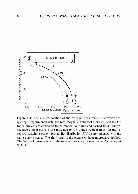
80 CHAPTER 4. PHASE ESCAPE IN EXTENDED SYSTEMS
520 530 540 550 56010
20
30
40
Resonance Current [µA]
Res
onan
t fre
quen
cy ω
0 ωP /
(2 π
)[G
Hz]
0 Oe
0.2 Oe I c(0
Oe)
I c(0.2
Oe)
I
P(I
)
ν=36GHz, H=0
Sample: AJJ-VAV
Figure 4.4: The current position of the resonant peak versus microwave fre-quency. Experimental data for zero magnetic field (solid circles) and 0.2 Oe(open circles) are compared to the model (solid line and dashed line). The re-spective critical currents are indicated by the dotted vertical lines. In the in-set two switching-current probability distribution P (Isw) are indicated with thesame current scale. The right peak is the escape without microwave applied.The left peak corresponds to the resonant escape at a microwave frequency of36 GHz

4.3. RF INDUCED DECAY 81
−4 −2 0 2 445
50
55
60
65
70
75
magnetic field H [Oe]
Ω0 ω
P/ (
2 π)
[GH
z]
Sample: AJJ-VAV
Figure 4.5: Fielddependence ofzero bias oscil-lation frequencyΩ0 extractedform measureddata (error bars),Ω0(H) calculatedfrom Ic(h) usingthe VAV model(dashed line) andΩ0(H) of thesmall-junctionmodel (dottedline).

82 CHAPTER 4. PHASE ESCAPE IN EXTENDED SYSTEMS
4.4 Thermal Activation Measurements on ShortRings and the Crossover to the QuantumRegime
We performed phase escape distribution measurements on sample AJJ-SHORT(see appendix C). The switching current, calculated numerically using the har-monic approximation method compares well to the experimentally determinedmean switching current in Fig. 4.6. The corresponding standard deviation, forfields up to 200 µT is plotted in Fig. 4.7, where the scaling versus the mag-netic field is compared to the values of B found by the harmonic approximation.Foe low temperatures the scaling predicted for the thermal activation deviatesstrongly from the experimental results, indicating the crossover to the quantumregime. The absolute experimental values however required a correction to Bby a factor of approximately three. It may be supposed that the deviations aredue to either neglecting the two-dimensional nature of the potential, neglectingan additional degree of freedom by fixing the position of the localized phaseescape, or quantum corrections to the escape rate.
The procedure described in sec. 4.1 can be used to calculate the prefactorand the exponent of the potential scaling in Eq. (4.10) numerically. In the limitof a small Josephson junction, a scaling like that of the vortex case is expected.Whereas in the vortex case, the junction radius enters into the ratio of the poten-tial barrier height and the depinning current
Uγcr
=23
√2E02r2π (4.24)
in the small junction case, we find using Eq. (1.11)
U = 2EJ23
√2 = 2IC
23
√2Φ0
2π. (4.25)
Yet, the relation2πrE0 = EJ (4.26)
holds, too. When using this on Eq. (4.24) to rewrite the potential barrier in termsof EJ, we find
U = γcr2EJ23
√2 = 2γcrIC
23
√2Φ0
2π. (4.27)
Since γcrIC is nothing else but the switching current, a junction with a vortextrapped resembles Eq. (4.25) from the viewpoint of the relation between the po-tential barrier height and the switching current. The difference between the cases

4.4. THERMAL ACTIVATION AND QUANTUM REGIME 83
Figure 4.6: Themeasured meanswitching cur-rent on sample(AJJ-SHORT(see appendix C))as used in theprevious chapterfor the vortexactivation mea-surements. Alength of 3.5λJ
was assumedto calculate theline using theharmonic ap-proximation; anoffset in the fieldand a self-fieldcorrection factorwere chosen tomatch the data.
−200 −100 0 100 2000
50
100
150
B[µT]
I switch
[µA
]
Sample: AJJ-SHORT
is the small oscillation frequency, which is influenced by the junction length. Theother parameters (normalized ramp rate, damping) are the same be the same asfor the vortex case, and B which depends logarithmically on these parameters, isthe same. Hence it is possible to compare the ratio of the saturation temperaturefor the vortex case, discussed in sec. 3.5 directly to the saturation temperatureof the small junction case. The ratio of the unbiased potential barrier U and thesmall unbiased small oscillation frequency suffices for comparing the secondfactor in Eq. (3.28). The small oscillation frequency of a vortex is given by
Ω0 =1r
√2π
8γ
γcr, (4.28)
of a SJJ by
Ω0 =√
γ
γcr. (4.29)
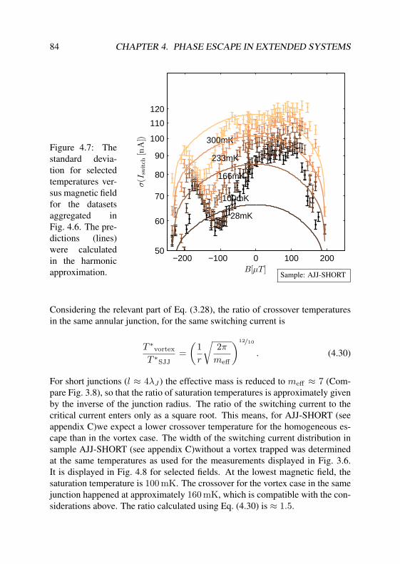
84 CHAPTER 4. PHASE ESCAPE IN EXTENDED SYSTEMS
Figure 4.7: Thestandard devia-tion for selectedtemperatures ver-sus magnetic fieldfor the datasetsaggregated inFig. 4.6. The pre-dictions (lines)were calculatedin the harmonicapproximation.
−200 −100 0 100 20050
60
70
80
90
100
110
120
B[µT]
σ(I
switch
[nA
])
28mK
100mK
166mK
233mK
300mK
Sample: AJJ-SHORT
Considering the relevant part of Eq. (3.28), the ratio of crossover temperaturesin the same annular junction, for the same switching current is
T ∗vortex
T ∗SJJ
=(
1r
√2π
meff
)12/10
. (4.30)
For short junctions (l ≈ 4λJ ) the effective mass is reduced to meff ≈ 7 (Com-pare Fig. 3.8), so that the ratio of saturation temperatures is approximately givenby the inverse of the junction radius. The ratio of the switching current to thecritical current enters only as a square root. This means, for AJJ-SHORT (seeappendix C)we expect a lower crossover temperature for the homogeneous es-cape than in the vortex case. The width of the switching current distribution insample AJJ-SHORT (see appendix C)without a vortex trapped was determinedat the same temperatures as used for the measurements displayed in Fig. 3.6.It is displayed in Fig. 4.8 for selected fields. At the lowest magnetic field, thesaturation temperature is 100 mK. The crossover for the vortex case in the samejunction happened at approximately 160 mK, which is compatible with the con-siderations above. The ratio calculated using Eq. (4.30) is ≈ 1.5.
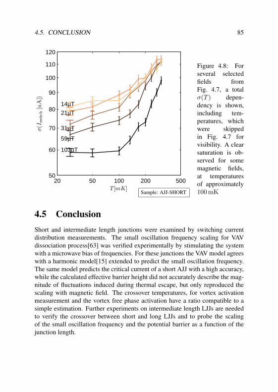
4.5. CONCLUSION 85
20 50 100 200 50050
60
70
80
90
100
110
120
T[mK]
σ(I
switch
[nA
])
14µT
21µT
31µT
59µT
103µT
Sample: AJJ-SHORT
Figure 4.8: Forseveral selectedfields fromFig. 4.7, a totalσ(T ) depen-dency is shown,including tem-peratures, whichwere skippedin Fig. 4.7 forvisibility. A clearsaturation is ob-served for somemagnetic fields,at temperaturesof approximately100 mK
4.5 ConclusionShort and intermediate length junctions were examined by switching currentdistribution measurements. The small oscillation frequency scaling for VAVdissociation process[63] was verified experimentally by stimulating the systemwith a microwave bias of frequencies. For these junctions the VAV model agreeswith a harmonic model[15] extended to predict the small oscillation frequency.The same model predicts the critical current of a short AJJ with a high accuracy,while the calculated effective barrier height did not accurately describe the mag-nitude of fluctuations induced during thermal escape, but only reproduced thescaling with magnetic field. The crossover temperatures, for vortex activationmeasurement and the vortex free phase activation have a ratio compatible to asimple estimation. Further experiments on intermediate length LJJs are neededto verify the crossover between short and long LJJs and to probe the scalingof the small oscillation frequency and the potential barrier as a function of thejunction length.

86 CHAPTER 4. PHASE ESCAPE IN EXTENDED SYSTEMS

Chapter 5
Double-Well Potentials inLong Josephson Junctions
One of the objectives of this work is to examine the possibility of creating adouble-well potential for vortices. Such a potential should be suitable for creat-ing a qubit based on spatially distinct vortex states. The realization of a double-well potential in a long Josephson junction requires a method to create a lo-calized potential barrier. During the qubit operation both, barrier height andsymmetry of the potential must be tunable independently.
A crucial point is that the quantum state of a system decoheres due to dissi-pation, which manifests as a rapidly increasing degree of entanglement with theoscillators forming the heat bath. The criteria for coherent evolution depend ondamping and temperature. In a quartic double well potential with ohmic dissipa-tion, the minimum requirement for observing any coherent effect is given [95],[73, P. 322] by
αc =meffη∆x0
2π~<
12, (5.1)
where ∆x0 is the separation between the classical equilibrium positions of theparticle in the double well. The value αc is a dimensionless coupling strengthof the system to the bath. In the case of long Josephson junctions, this conditiontranslates to a simple criterion for a working qubit
∆x0 ~η. (5.2)
87
88 CHAPTER 5. DOUBLE-WELL POTENTIALS
The simple relation in Eq. (5.1) is replaced by the stronger criterion in Eq. (5.2),since Eq. (5.1) corresponds to the condition of observing any coherent effect,(including a single coherent oscillation), while for a working quantum computa-tion system, many coherent oscillations are required.
Since the bath is not only entangling with the qubit, but subjected to a ther-mal distribution of its own state, there also exists a condition on temperature.This condition is related to the level splitting ∆0 of the lowest energy eigen-states in the double well and the average thermal energy kBT of a fluctuator inthe bath
αckBT
∆0 1. (5.3)
In a hand-waving interpretation, Eq. (5.1) determines how quickly quantum in-formation leaks to the heat bath, while Eq. (5.3) determines how much quantuminformation per unit time is transferred from the heat bath to the qubit. It isstriking that the different factors in Eq. (5.1) and Eq. (5.3) depend on differentsteps of the production of the qubit. The damping η is set by the quality of thedielectric in the junction and its surroundings, ~ is set by the lithographic res-olution. The energy scale kBT by the cryogenic equipment. So it is up to thedesigner of the potential, and the experimenter, to set δx0 and ∆0 appropriately.In order to fulfill Eq. (5.1) it is essential that both δx0 and ∆0 are controlled atthe time of the experiment. To operate a qubit, it must be prepared in the clas-sical regime by intentionally violating Eq. (5.1) while reducing of the coupling,thereby projecting the state. The operation frequency of the control circuit is setby the coherent oscillation period τcoh = ~/∆0. During a time considerablysmaller than τcoh, the control circuit changes the qubit’s potential from a regimefulfilling Eq. (5.1) and Eq. (5.3) to a regime where Eq. (5.1) is violated and ∆0
vanishes, projecting the qubit state to a classical state. When reading out theclassical state to which the original qubit’s state has been projected it is essentialthat no thermal activation takes place in the meantime1.
In long Josephson junctions there exist several independent ways of gener-ating potentials for vortices. Among the terms in Eq. (1.43) we group HJ andHL, which both contribute to the vortex rest mass and HH, the external mag-netic field interaction energy. The first energy term HJ +HL is parametrized asby the junction width, the critical current density jc and the junction curvature.Variation of the rest mass along the junction can be used to form a potentialfor the vortex. Previously microshorts, small areas of increased critical currentand microresistors, small areas of decreased critical current, density were the-
1Due to possibly different time scales, this condition is independent from Eq. (5.3).

5.1. PARASITIC POTENTIALS 89
oretically discussed in relation to this [96, 82]. Although it is difficult to varythe critical current density jc as a function of the position using a standard tri-layer process, microshort qubits based on this microshorts have been proposed[18]. Relaxation and decoherence times for vortex qubits based on microresis-tors were estimated [97], considering the 1
f fluctuations of the critical currentand effect of temperature.
An alternative approach is based on varying the junction width [19, 98]. Thisthesis presents the first results of experiments studying the effect of localizedwidth changes designed to produce a double-well potential.
The HH term is parametrized by the local external magnetic field. A lo-calization can be created either by generating a local magnetic field, or an ex-ternal homogeneous field, where the vortex-field interaction is defined by theangle between the junction’s centerline and the external magnetic field. To cre-ate a double-well potential using this method, heart-shaped Josephson junctions[13, 10, 11, 12] have been proposed. It is worth mentioning that a curvaturechange causes parasitic potential barriers in heart-shaped junction. This is dis-cussed briefly using a model for a curved Josephson junction in Ref. [17] in thelimit of junction widths smaller than a Josephson length.
The bias current interaction term Hγ in Eq. (1.43) can be used to tilt thepotential. To observe coherent quantum effects, a particularly well controlledpotential tilt is needed, since its fluctuations determine the speed of the quantummechanical phase evolution.
5.1 Parasitic Potentials in Heart-Shaped Joseph-son Junctions
One possibility to shape a controllable double well potential is to engineer thedirection of the centerline of the junction such that the vortex interaction withthe external magnetic field depends on vortex position. Bending the junction di-rection changes the mutual inductances of the junction segment with each of theorthogonal (x,y) external in-plane magnetic field components. Bistable statesin heart-shaped Josephson junctions have been demonstrated in Ref. [11, 12].Regrettably, the spatial separation between the classical states in the two poten-tial minima, is set at production time by the geometry and critical current of thejunction[10], which is imprecisely produced. For a normalized Plancks constant~ on the order of 10−4 to 10−3 ,corresponding to junctions of µm to moderatesub-µm width, it seemed reasonable to create a systematic spread of the junctionparameters at design time to manufacture an acceptable yield of junctions fulfill-
90 CHAPTER 5. DOUBLE-WELL POTENTIALS
ing Eq. (5.1) and simultaneously capable of considerable tunneling rates[10]. Aelectron beam micrograph of a junction designed for a test in the thermal regimeis shown in Fig. 5.1.
The potential created by a curved segment in a long Josephson junction with-out magnetic field is derived in Ref. [17]. If the junction width is smaller than asingle Josephson length, the effect of the curvature is described by first order per-turbation theory, equivalent to the interaction of a vortex with a magnetic field.The parasitic potential is generated by the variation of the energies associatedwithHJ andHL. The static vortex solution does not only fulfill the sine-Gordonequation, but also stores equal energy densities in the Josephson coupling andthe magnetic field. Since both energy density distributions contribute equally tothe rest mass, and are proportional to the junction width, it is possible to definethe “rest mass profile” µ of a static vortex at position x0 as:
µ(x0) = 4sech2(x0). (5.4)
Using this, the vortex rest mass m takes the form of a simple convolution
m(x0) = µ(x) ∗ µ(x− x0), (5.5)
where µ(x) is the mass density per unit length and per squared magnetic fieldunit, normalized to E0
µ(x) =
∫ w
012ϕx
2 + (1− cos ϕ)dy∫ w0
012ϕx
2 + (1− cos ϕ)dy. (5.6)
Compared to the case of convolution of the magnetic field with the magnetic fieldsech-kernel [48, 99, 10], the rest mass convolution sech2-kernel is narrower,corresponding to a higher curvature for the same potential barrier height. Acomparison between both kernels is shown in Fig. 5.2.
The rest mass density µ is determined by the junction shape. This is due tothe deformation of the fluxon in comparison to the one dimensional sine Gor-don equation model. For the heart-shaped Josephson junctions discussed in thisthesis, only a small part of the junction has a radius small enough to changethe potential energy considerably. In the micrograph in Fig. 5.1, all parts of thejunction except for the bend in the enlarged region are assumed to have infiniteradius. In this case [17], the local rest mass density of the field in normalizedunits takes the form
µ(x) =(
R
wlog
2R + w
2R− w− 1)
︸ ︷︷ ︸µc
Θ(a + x) + Θ(a− x)2
+ 1, (5.7)

5.1. PARASITIC POTENTIALS 91
Bottom electrode
junction definition
top electrode
(2)(1)
Hext
β
Figure 5.1: Micrograph of a sample AJJ-HEART2 (see appendix C). The ex-ternal magnetic field orientation and the designed vortex states (1) and (2) areindicated. The enlarged region is intended to provide a magnetic field dependentbarrier. The inset shows an enlarged region, in which the junction curvature ishigh.
where x = −a is the beginning, and x = a the end of the curved region. InFig. 5.1, a = rβ, the. The convolution of the sech2 kernel with the step-functioncan be carried out analytically (since the integral of the kernel is known), yield-ing the first-order perturbation potential
U(x0) = µctanh(x0 − a)− tanh(x0 + a)
2. (5.8)
In the junctions AJJ-HEART1, AJJ-HEART2, AJJ-HEART3 (see appendix C),R = 2 µm, w = 3.5 µm, and λJ = 14 µm, for angles β of 26,37, and43. The influence of lateral vortex deformation[17] is neglected by setting thevariation parameter B from[17] to zero. To determine whether a lateral variationof the phase should be considered, the deformation energy for a vortex[17, seeEq.27] is calculated to first order by
U =4π4
24w2B2, (5.9)

92 CHAPTER 5. DOUBLE-WELL POTENTIALS
−5 0 50
0.1
0.2
0.3
0.4
0.5
0.6
0.7
0.8
0.9
1
x −x0
µ(x−x0)
sech
sech2
Figure 5.2: Thesech2(x) con-volution kernel(dashed line), tobe convolutedwith the vortexmass profile iscompared to thesech(x)-kernel,associated withthe vortex mag-netic field profile.
where B is the first harmonic component of the lateral deformation[17]. Thismeans that the the vortex shape remains unperturbed, and B = 0 is an adequateapproximation. If w < 1, the energy attributed to this deformation is high.
Fig. 5.3 contains measured depinning currents, minimized by varying exter-nal magnetic fields as well as the depinning current obtained from the convolutedpotential Eq. (5.8) as a function of the angle β.
Some measurements not included in Fig. 5.3 contain other pinning sourceslike Abrikosov vortices. These are identified by too large zero field pinning cur-rent, or a changing zero-field depinning current during repeated measurements.These measurements were carried out without injecting vortices. Theory andexperiment agree acceptably, considering that neither the effect of the irregu-lar finite idle region at this location on the magnetic field distribution is knownnor the mask alignment error, which causes an asymmetry in the idle regionwidth(see Fig. 5.1, enlarged region) is taken into account. Both effects couldgive rise to a moderate change in the total inductance along the junction. Usingthe same parameters as in Fig. 5.3, the potential barrier height at zero field canbe derived. The result is shown in Fig. 5.4. For a junction of width 3.5 µm,jc = 1 kA/cm2 and radius of curvature 2 µm, this barrier dominates the mag-

5.1. PARASITIC POTENTIALS 93
25 30 35 40 450
100
200
300
400
500
600
β [o]
min
(Ic [µ
A])
Figure 5.3: Theminimal pin-ning currents,determined with-out active statepreparation, forjunctions of dif-ferent bendingangle β. The lineis the predictionfor the pinningcurrent usingthe estimationgiven Ref. [17],a radius of 2 µmand a junctionwidth of 3.5 µmat a critical cur-rent density ofjc = 1 kA/cm2.Dots/open circlescorrespond todifferent currentpolarities.
netic field induced barrier even at moderate fields. This parasitic barrier makesit impossible to observe thermal activation in any of the produced junctions. Toachieve a working qubit, barrier heights on the order of one Kelvin were in-tended. Thus the the possibility of characterizing the magnetic field inducedbarrier in the thermal regime on junctions with a spatial scale achievable usingphoto-lithography is excluded. While this hinders systematic progress on devel-oping a working vortex qubit based on a barrier formed by magnetic field, theconcept may still work in the limit of very narrow junctions. Evaluating Eq. (5.7)for different junction widths shows that, for a fixed radius of 2 µm at a criticalcurrent density of jc = 1 kA/cm2, the relative size of the effect is reduced by twoorders of magnitude for a junction of a width of ≈ .2 µm.

94 CHAPTER 5. DOUBLE-WELL POTENTIALS
25 30 35 40 451100
1200
1300
1400
1500
1600
1700
1800
1900
2000
2100
Bar
rier
heig
ht [K
]
β [o]
Figure 5.4: Thepotential barrierheight in Kelvin,caused by thecurvature only,versus angle β.

5.2. LITHOGRAPHIC MICROSHORTS 95
5.2 Lithographic MicroshortsA microshort is a small area in a long junction, which has an increased criticalcurrent density. In a one-dimensional model, this means that the critical currentdensity along the length of the junction is modulated. Usually this is thought tobe caused by a variation of the barrier thickness, as sketched in Fig. 5.5. In thesimple case that the modulation has a spatial extent which is small in comparisonto λJ , it can be described by a δ-like inhomogeneity of the critical current:
jc(x) = (1 + µδ(x− xµ))jc0 (5.10)
Here xµ is the position of the microshort and jc0 is the unperturbed criticalcurrent density. µ describes the relative strength of the microshort, which is theproduct of the change in the critical current density with the spatial extent ofthis change. Such inhomogeneities contribute a perturbation to the sine-Gordonequation
ϕxx − ϕtt = (1 + µδ(x− xµ)) sin(ϕ), (5.11)
which was discussed in the perturbation theory of Ref. [47]. For the motion of avortex the effective potential was derived in to be
U = 2µsech2(x− xµ). (5.12)
If µ is negative it corresponds to an increased thickness of the barrier, and alocal decrease of the critical current density. The whole perturbation is calleda microresistor in this case. Few instances of long Josephson junctions witha spatially artificially modulated critical current density have been previouslyrealized experimentally [100, 101]. All previous experimental realizations ofmodulated critical current density involved regions of zero critical current den-sity created by replacing the trilayer with an insulating barrier (insulator-typemicroresistors). Fluctuation induced activation on an annular junction contain-ing a single insulator-type microresistor to create a vortex pinning potential werereported in [8]. A very relevant result of Ref. [8] is the fact that the capacitancechange of an insulator-type microresistor is considerable and plays a role in theexperiment. At the structuring resolutions available (on the order of 1 µm for anreliable insulation), one finds the minimal potential depth of the well to be onthe order of 500 K for jc = 1 kA/cm2 . Still, since the potential is convolutedwith the fluxon shape, the use of spatially close insulator-type microresistors tocreate a small barrier in between could be feasible. This would result in a dou-ble well potential, however up to now the preparation and readout of bistablestates in such a structure has not been demonstrated. Without considering the

96 CHAPTER 5. DOUBLE-WELL POTENTIALS
jc1
xjc2
Figure 5.5: Aside view of astandard mi-croshort. In astandard mi-croshort thebarrier thicknessis spatially mod-ulated to changethe overlap of theorder parametersbelonging to eachelectrode.
experimental realization, the observation of quantum effects on microshorts asbarriers was theoretically described earlier [81]. Specifically the tunneling of avortex through a single barrier and the resonant tunneling through a double bar-rier formed by two microshorts was considered there. Using a long Josephsonjunction containing a microshort in an external magnetic field as a qubit wasproposed in Ref. [18]. No trilayer process allowing the reproducible productionof microshort junctions is available. The difficulty is that the trilayer is formedby oxidation, a process very sensitive to external parameters, especially the par-tial pressure of oxygen. Hence it is difficult to perform the lithographic step,required for spatially defining the areas of increased or reduced critical currentdensity.
The rest of this chapter examines an alternative approach to the problem offorming a well defined microshort-like structure with which to build a vortexqubit. We use local variation of the junction width to create a localized barrier.Such width modulation was considered before [19], with the intention of creat-ing a microscopic ratchet potential in one-dimensional Josephson junctions. Tothe authors knowledge no working realization of width modulated junctions waspresented. Our junction design is laid out in Fig. 5.6. In the subsequent sectionssuch width modulated junctions are discussed and the first experimental resultsare presented.
The width variation is defined by ∆w(x) = w(x) − w0, where w0 denotesthe unperturbed width. In the junction designs tested experimentally ∆w(x) was

5.2. LITHOGRAPHIC MICROSHORTS 97
~H
y
x
(2)(1)
Figure 5.6: Anannular Joseph-son junctionsactive area, withlaterally appliedmagnetic field.The finite re-gion of largerwidth, used toform the doublewell potential,is enlarged. Thestable positionsof the fluxonswith applied ex-ternal magneticfield are indicatedby (1) and (2).
defined by a step function
w(x) = w0 + wmsΘ(|x| − lms/2), (5.13)
where wms is the extra width at the step, and lms the length of the microshort.The complete layout is shown in detail in Fig. 5.7. In our case, wms = 0.5 µm,and lms = 2µm, and w0 = 3µm. If the maximum width of the junction issmaller than λJ , the phase is laterally constant ϕ(x, y) = ϕ(x). Hence thecomplete model is still defined by a one-dimensional field equation of motion.
The most important difference in the derivation of the field equation of mo-tion for a long junction including a microshort is that the whole Lagrangian ismultiplied by a single factor
L =(
1 +∆w(x)
w0
)(12ϕx
2 + (1− cos ϕ)− ϕt) . (5.14)
A perturbed equation of motion is found by applying the Lagrangian formalism
wx(x)w(x)
ϕx = sinϕ− ϕxx + ϕtt (5.15)

98 CHAPTER 5. DOUBLE-WELL POTENTIALS
wms = 0.5 µmlms = 2 µm
w0 = 3 µmFigure 5.7: Thespecific layout ofthe microshort re-gion for the junc-tion used in theexperiments.
It is striking that the LHS of this equation of motion has the same function asa bias current perturbation to a SGE. The physical meaning is obvious: Thecurrent flowing trough the junctions electrode is proportional to its width andthe phase gradient. It is easy to perform the thought experiment of connectingseveral identical junctions in parallel, each threaded by the same magnetic field.If the magnetic field at a given point changes smoothly, this means that at aninductance change the lateral current along the electrode will change; since theKirchhoff law holds, this means that current flows through the junction. Suchparametric inductance changes in sine-Gordon systems have been consideredbefore [69, 19]. Usually it is assumed that the change is slow in comparison tothe characteristic length. In this case the first-order perturbation theory equiva-lent to [47] can be applied. The derivative of the junction width wx(x) is in ourdesign is as sharp as the production process allows. It was not possible to ex-amine the final junction using electron beam microscopy, since the dimensionsof the lithographic microshort were on the order of the thickness of the metal-ization and insulation layers above, so that the real wx(x) is unknown. Hencethe data needed to determine if wx(x) is small enough to ignore the influenceof the perturbation on the fluxon shape is lacking. Assuming that the phase pro-file of a vortex located at x0 is unchanged by the perturbation (equivalent toassuming a small wx(x)) it can be substituted it into the changed energy den-sity H = H0w(x)/w0. Again, from the relevant terms in Eq. (1.43) we groupHJ and HL, which are the only two terms which play a role for an unbiased,magnetic field-free Josephson junction.
Since lms is shorter than the Josephson length the effect of the modulation is

5.2. LITHOGRAPHIC MICROSHORTS 99
approximated in first order perturbation theory by
w(x)w0
= 1 + δ(x)µms, (5.16)
where µms is the total junction area in the extra region. For this case the potentialpredicted by the perturbation theory is given by
U(x0) = 4µmssech2(x0) (5.17)
5.2.1 Bistable States in Microshort JunctionsThis potential can be added to the effective potential described by Eq. (1.69),created by a magnetic field of strength ~hext,V in the vertical direction and ~hext,H
in the horizontal direction, and a driving bias current term γ, resulting in thepotential
U(x0) = 4µmssech2x0 − 2π
(γx0 − cos
(x0
r
)~hext,V + sin
(x0
r
)~hext,H
).
(5.18)The position of the microshort is set to be x0 = 0. If a vertical magnetic field(oriented as in Fig. 5.6) is applied, Eq. (5.18) a double-well potential is created.For various vertical magnetic fields the resulting potential is plotted in Fig. 5.8.The barrier height of this potential is predetermined during design time by themicroshort strength µms. When a vertical magnetic field magnetic field is ap-plied, the barrier is reduced. In order to determine the criterion for zero barrierheight, it must be determined whether the potential given by Eq. (5.18) has aminimum or a maximum at x = 0. Obviously the slope at this point is 0, if~hext,H = 0. The criterion for a minimum or a maximum is given by the totalcurvature at this point; so the curvature of the magnetic field created potentialand the microshort created potential are added. We define the orientation ofthe vertical field so that ~hext,V > 0 for the orientation of the magnetic field inFig. 5.6. The criterion for the two curvatures adding to zero is thus given by
2π~hext,V
r2= 8µms. (5.19)
The critical magnetic field strength hext,cr at which the potential vanishes isgiven by
hext,cr =r28µms
2π(5.20)
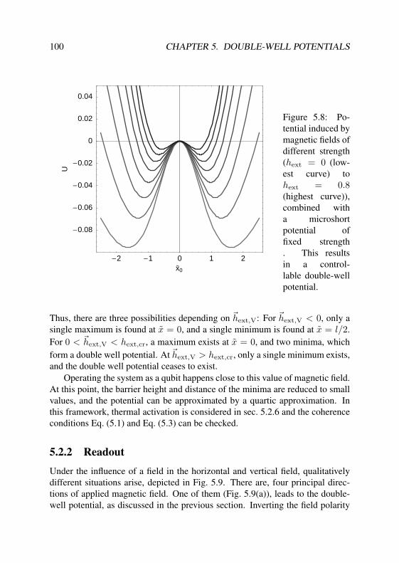
100 CHAPTER 5. DOUBLE-WELL POTENTIALS
-2 -1 0 1 2x0
-0.08
-0.06
-0.04
-0.02
0
0.02
0.04
U
Figure 5.8: Po-tential induced bymagnetic fields ofdifferent strength(hext = 0 (low-est curve) tohext = 0.8(highest curve)),combined witha microshortpotential offixed strength. This resultsin a control-lable double-wellpotential.
Thus, there are three possibilities depending on ~hext,V: For ~hext,V < 0, only asingle maximum is found at x = 0, and a single minimum is found at x = l/2.For 0 < ~hext,V < hext,cr, a maximum exists at x = 0, and two minima, whichform a double well potential. At ~hext,V > hext,cr, only a single minimum exists,and the double well potential ceases to exist.
Operating the system as a qubit happens close to this value of magnetic field.At this point, the barrier height and distance of the minima are reduced to smallvalues, and the potential can be approximated by a quartic approximation. Inthis framework, thermal activation is considered in sec. 5.2.6 and the coherenceconditions Eq. (5.1) and Eq. (5.3) can be checked.
5.2.2 Readout
Under the influence of a field in the horizontal and vertical field, qualitativelydifferent situations arise, depicted in Fig. 5.9. There are, four principal direc-tions of applied magnetic field. One of them (Fig. 5.9(a)), leads to the double-well potential, as discussed in the previous section. Inverting the field polarity

5.2. LITHOGRAPHIC MICROSHORTS 101
Figure 5.9: Thestable positionsin a microshortjunction, indi-cated by arrowsfor the four prin-cipal directionsof the magneticfield.
(Fig. 5.9(b)) leads to the situation where the magnetic field is repulsive at the po-sition of the microshort. So only a single stable position exists. Applying a fieldin the perpendicular direction (Fig. 5.9(c,d)) leads to the situation, where onestable position is (for a long Josephson junction) the magnetic field induced one.The microshort is far away, and its influence is practically zero. A second stableposition does exist, which is more obvious when comparing the correspondingpotentials depicted in Fig. 5.10. If the microshort pinning is strong enough, itcan locally compensate for the slope of the magnetic field induced potential andcreate a second minimum. Under horizontal field the potential shows neither anpoint-like symmetry nor an mirror symmetry. Still under the inversion of themagnetic field polarity the potential is mirrored, so that the situations (c) and (d)in Fig. 5.10 and Fig. 5.9 are equivalent, if the junction coordinate is reversed.This is more closely discussed in sec. 5.2.5.
Now we examine the depinning process further. The simplest situation is thesymmetric double well potential, plotted in Fig. 5.11. The figure also indicatesthe points of the maximum slope of the potential. If a vortex is trapped in eitherminimum, a bias current with a magnitude smaller than max(Ux/(2π)), where

102 CHAPTER 5. DOUBLE-WELL POTENTIALS
-10 -5 0 5 10x
-0.5
-0.25
0
0.25
0.5
0.75
1
U
HaL HcL HdL
HbL
Figure 5.10: Po-tentials for thefour magneticfield directionsindicated inFig. 5.9. Thecurves are des-ignated withthe correspond-ing letters fromFig. 5.9. Thejunction lengthis 20λJ , the mi-croshort strengthµms = 0.033.
max denotes the closest maximum in the positive direction is needed to free thevortex. If the bias current exceeds this value, the vortex is driven beyond thispoint. From there the vortex is accelerated by the bias current. This accelera-tion gives a rise to the kinetic energy of the vortex. The increase in velocity isproportional to the driving force and the distance the vortex travelled since de-pinning. So the total energy of the vortex is given by a straight line, which startsat the potential energy at the position of depinning and rises with a slope equalto the depinning force. Thus the tangent to the potential at the location of max-imum slope represents the total energy of the depinned vortex as a function ofposition. If this tangent does not intersect the potential a second time, the vortexovercomes all maxima of the potential, since its energy is the sum of its startingpotential energy and the energy gained from the driving force. Otherwise, thevortex is pinned again at the next maximum. Fig. 5.11 shows a situation, whereneither of the tangents cuts the potential again. A a vortex in either well is lib-erated at the corresponding current. Since the two critical currents are different,this can be used for readout of the state.
The two critical currents, corresponding to the microshort pinning potentialand the magnetic field induced pinning potential can be found numerically. Forthe case of zero magnetic field, the microshort depinning current can be calcu-

5.2. LITHOGRAPHIC MICROSHORTS 103
-7.5 -5 -2.5 0 2.5 5 7.5 10x
0
0.5
1
1.5
2
2.5U
Figure 5.11: De-pinning positionsin a symmetricpotential (dots).The lines are thetangents to thepotential in thesepoints. None ofthe tangents cutthe potential asecond time inthe direction ofdepinning.
lated analytically 2 to be
γcr = − 42π
µms
8√(
1− 2√5
) (1 + 2√
5
)5
. (5.21)
If the particle is trapped at the magnetic field barrier, it is depinned at
γcr = hext/r (5.22)
At small magnetic field, the two depinning currents differ strongly. Since themicroshort barrier disappears at the magnetic field determined by Eq. (5.19), ofthe corresponding well is reduced to zero at this field. There is no closed-formexpression for the depinning from this well as a function of magnetic field, but itis a monotonous function, so at some magnetic field the field induced depinningcurrent overcomes the microshort induced depinning current.
2Remove the root sech2 from the second derivative to find the equation for the positions of theabsolute maxima of the force sech(x0) = 2 tanh(x0).

104 CHAPTER 5. DOUBLE-WELL POTENTIALS
5.2.3 State Preparation
State preparation can be performed by the “shaker” method. This method makesuse of the fact that in general the retrapping of the system, after turning off thebias current, happens stochastically. A current is chosen to have a magnitude be-tween the microshort induced depinning current and the magnetic field induceddepinning current. A biascurrent pulse train, switching between zero current andthis current is applied to the junction (phase (1) in Fig. 5.12). If the system re-sides in the state of the lower pinning current, the vortex is depinned, otherwiseno switching happens. If retrapping happens stochastically, the vortex settles af-ter each pulse to the state of the higher depinning current with some probability.Thus, the probability of being in the state associated with the lower depinningcurrent decreases exponentially with the number of pulses.
5.2.4 Experimental Test of State Preparation and Readout
The overall experimental biasing sequence is depicted in Fig. 5.12. After thepreparation of the system in phase (1), phase (2) changes the magnetic fieldto suppress the potential. This is the phase where experiments are carried out.Before proceeding to these experiments, a test of the preparation and readoutscheme is done. The readout is done at the end of the sequence in phase (3)in Fig. 5.12 by a current ramp. If the magnetic field is chosen correctly, thesituation is as in Fig. 5.11, where the two pinned states of the vortex differ inthe depinning current, and can be read out. In order test the state preparationand readout, the pulse height in phase (2) is set to zero, and the magnetic field invertical direction is swept.
The result of this preparation and readout, without the suppression pulse, isdisplayed in Fig. 5.13, where the different symbols denote the polarity of theshaker pulses. The potential without bias current is symmetric around the mi-croshort position; inverting the polarity of the shaker pulses just tilts the potentialin the other direction. The same applies to the readout. A state pinned by themicroshort under positive bias current polarity is the same state, as appears tobe pinned by magnetic field under negative bias polarity. Using shaker pulsesand reading out in the same bias current polarity we will find the higher of bothdepinning currents, while, when reading out in the opposite polarity we expectto find the lower depinning current. Qualitatively the predicted existence of thebistable states for the positive field polarity is verified in Fig. 5.13, including therelations between the polarity of readout and shaker pulses. This identifies themicroshort-like depinning on one polarity to be associated with the same state
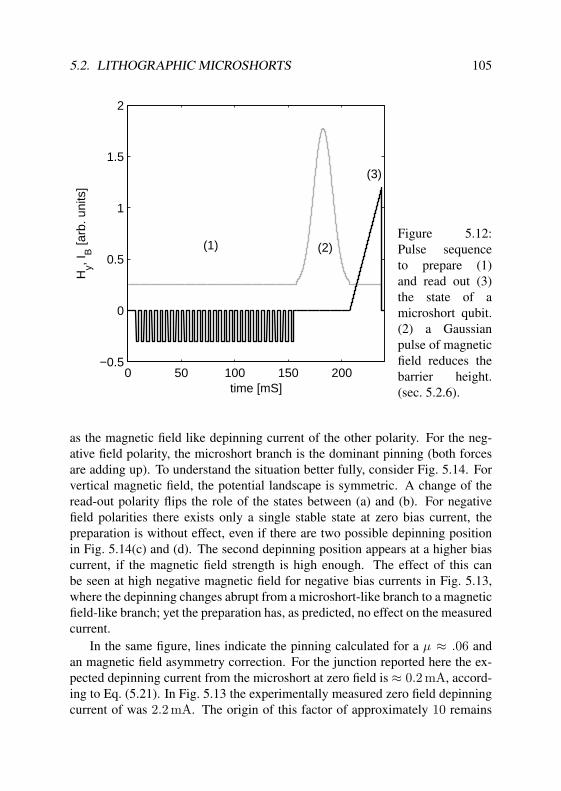
5.2. LITHOGRAPHIC MICROSHORTS 105
0 50 100 150 200−0.5
0
0.5
1
1.5
2
time [mS]
Hy, I
B [a
rb. u
nits
]
(1) (2)
(3)
Figure 5.12:Pulse sequenceto prepare (1)and read out (3)the state of amicroshort qubit.(2) a Gaussianpulse of magneticfield reduces thebarrier height.(sec. 5.2.6).
as the magnetic field like depinning current of the other polarity. For the neg-ative field polarity, the microshort branch is the dominant pinning (both forcesare adding up). To understand the situation better fully, consider Fig. 5.14. Forvertical magnetic field, the potential landscape is symmetric. A change of theread-out polarity flips the role of the states between (a) and (b). For negativefield polarities there exists only a single stable state at zero bias current, thepreparation is without effect, even if there are two possible depinning positionin Fig. 5.14(c) and (d). The second depinning position appears at a higher biascurrent, if the magnetic field strength is high enough. The effect of this canbe seen at high negative magnetic field for negative bias currents in Fig. 5.13,where the depinning changes abrupt from a microshort-like branch to a magneticfield-like branch; yet the preparation has, as predicted, no effect on the measuredcurrent.
In the same figure, lines indicate the pinning calculated for a µ ≈ .06 andan magnetic field asymmetry correction. For the junction reported here the ex-pected depinning current from the microshort at zero field is ≈ 0.2 mA, accord-ing to Eq. (5.21). In Fig. 5.13 the experimentally measured zero field depinningcurrent of was 2.2 mA. The origin of this factor of approximately 10 remains
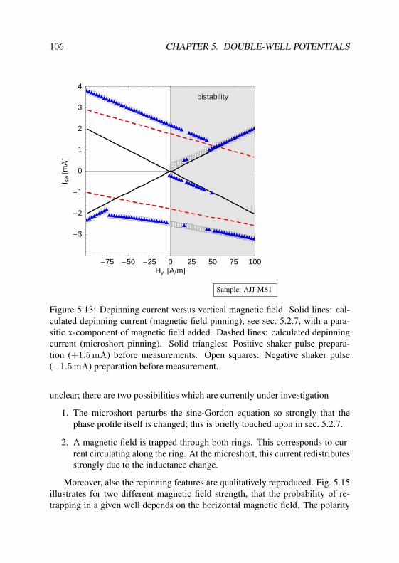
106 CHAPTER 5. DOUBLE-WELL POTENTIALS
-75 -50 -25 0 25 50 75 100Hy @AmD
-3
-2
-1
0
1
2
3
4
I sw@m
AD
bistability
Sample: AJJ-MS1
Figure 5.13: Depinning current versus vertical magnetic field. Solid lines: cal-culated depinning current (magnetic field pinning), see sec. 5.2.7, with a para-sitic x-component of magnetic field added. Dashed lines: calculated depinningcurrent (microshort pinning). Solid triangles: Positive shaker pulse prepara-tion (+1.5 mA) before measurements. Open squares: Negative shaker pulse(−1.5 mA) preparation before measurement.
unclear; there are two possibilities which are currently under investigation
1. The microshort perturbs the sine-Gordon equation so strongly that thephase profile itself is changed; this is briefly touched upon in sec. 5.2.7.
2. A magnetic field is trapped through both rings. This corresponds to cur-rent circulating along the ring. At the microshort, this current redistributesstrongly due to the inductance change.
Moreover, also the repinning features are qualitatively reproduced. Fig. 5.15illustrates for two different magnetic field strength, that the probability of re-trapping in a given well depends on the horizontal magnetic field. The polarity

5.2. LITHOGRAPHIC MICROSHORTS 107
Figure 5.14: Depinning positions in a microshort Josephson junction. The yel-low arrows mark the driving bias force. Note that for magnetic field pinningthe fluxon is depinned at a point a quarter of the junction length away from thelocation of the unbiased minimum. The depinning from the microshort happensat a comparatively constant location, nearly independent of the magnetic fieldstrength. The signature of a localized pinning potential is the symmetry of theobserved depinning process. While for vertical field direction (parallel to thesymmetry axis) the same absolute values of depinning currents are expected forthe different bias current polarities (a) and (b), in the case of the horizontal mag-netic field, an opposite bias current requires the magnetic field polarity also tobe reversed to achieve the same absolute value of depinning current, like forthe pair (e)-(h). The situations (a),(b),(e),(h) correspond to observable bistablestates. In (g) and (f) only a single stable state exists. For (c) and (d) the distancebetween the location of depinning from the magnetic field induced potential istoo close to the next maximum, which is not overcome.

108 CHAPTER 5. DOUBLE-WELL POTENTIALS
-5 0 5 10 15 20x
-0.75
-0.5
-0.25
0
0.25
0.5
0.75
1
U
Figure 5.15: For two dif-ferent horizontal magneticfield strengths, the poten-tials are plotted (offset forgreater visibility), includingthe vortex energy trajecto-ries. The depinning de-pends on the strength of themagnetic field, since at thelower magnetic field the mi-croshort created maximumis not overcome. Hence onlythe depinning from the mi-croshort can be observed be-low a certain field threshold.In order to visualize the peri-odicity, the potential is drawbeyond the junction bound-ary.
chosen is equivalent to situations (e) and (h) in Fig. 5.14. The opposite polarities(f) and (g) in the same figure are shown in Fig. 5.17. In cases (f) and (g) thewell from which the vortex escapes is more shallow, so that a vortex depinnedfrom the microshort will be repinned in the magnetic field potential well. Theseconsiderations agree with the observations of bistable states inFig. 5.16.
5.2.5 Symmetry of the Patterns
As done in the previous section, the depinning processes can be also understoodqualitatively for the horizontal magnetic field direction. The expected approxi-mate depinning positions for all four field directions are illustrated in Fig. 5.14.Under reversal of both the bias current polarity and the horizontal magnetic fieldpolarity, the depinning current stay the same. When viewing at the horizontalmagnetic field pattern in Fig. 5.16 to the schematic situations, one finds that thesymmetry is matched.

5.2. LITHOGRAPHIC MICROSHORTS 109
-75 -50 -25 0 25 50 75 100Hx @AmD
-3
-2
-1
0
1
2
3
4
I sw@m
AD
HeL
HhL HfL
HgL
Sample: AJJ-MS1
Figure 5.16: De-pinning currentsversus horizontalmagnetic field.The line stylesand symbolstyles have thesame meaningas in Fig. 5.13.Gray diamondsare from anunprepared mea-surement.
5.2.6 Thermal Activation over a Suppressed BarrierTo examine the thermal and quantum activation over the bistable potential wellat zero bias current, a quartic approximation to the potential is used. This isderived from the Taylor series of the magnetic field potential, and the microshortpotential, respectively. At hext ≈ hext,cr (see Eq. (5.20)) the potential is wellapproximated by a quartic polynomial.
U = ax20 + bx4
0 − 2πγx0 (5.23)
where for the case of the (zeroth order) microshort potential, a =2π 1
2r2 (−hext +hext,cr) and b = 23µms. The unbiased barrier height evaluates to
U =a2
4b=
(−hext + hext,cr)2π2
4r4µms(5.24)
and the small oscillation frequency inside a single well to
Ω0 =√
2a
meff= 2
√π
√hext,cr
meffr2
√1− hext
hext,cr. (5.25)

110 CHAPTER 5. DOUBLE-WELL POTENTIALS
-5 0 5 10 15
0
0.2
0.4
0.6Figure 5.17: In anpotential, equiva-lent to Fig. 5.15,but with oppo-site magneticfield polarity thepinning well isslightly moreshallow, allow-ing only theobservation ofthe microshort-pinned state. Inorder to visualizethe periodicity,the potential isdraw beyondthe junctionboundary.
For a fixed value of b = 0.03, both expressions are plotted in Fig. 5.18 for smalla.
As a function of the control parameter a, the thermal switching rate of thesystem across the well in one direction is estimated in the underdamped limit as
Γth = Bη exp(−B), (5.26)
where B = U/kBT In Fig. 5.19 the result for parameters, similar to those forthe experiments is shown for an assumed damping of η = 10−5 and a temper-ature of 100 mK. To perform thermal activation between the wells a Gaussianmagnetic field pulse (see phase (2) in Fig. 5.12) suppresses the barrier. Thespecific parameters cannot be determined, as no matching analytic formula forthe potential is known. Substituting the rate (Fig. 5.19) into Eq. (2.5) and inte-grating numerically yields the probability of the particle to pass over the barrier.Depending on temperature, for a damping of η = 10−5, Fig. 5.20 displays thecalculated and the experimentally determined probability of the system havingswitched on the Gaussian height for temperatures between 100 mK and 900 mK.Depending on the temperature , the particle is activate with a certain probability
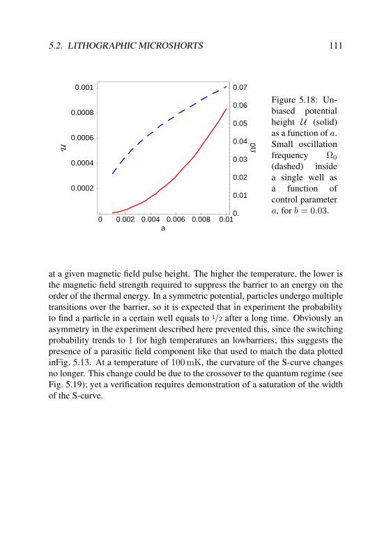
5.2. LITHOGRAPHIC MICROSHORTS 111
0 0.002 0.004 0.006 0.008 0.01a
0.0002
0.0004
0.0006
0.0008
0.001
U
0.
0.01
0.02
0.03
0.04
0.05
0.06
0.07
W0
Figure 5.18: Un-biased potentialheight U (solid)as a function of a.Small oscillationfrequency Ω0
(dashed) insidea single well asa function ofcontrol parametera, for b = 0.03.
at a given magnetic field pulse height. The higher the temperature, the lower isthe magnetic field strength required to suppress the barrier to an energy on theorder of the thermal energy. In a symmetric potential, particles undergo multipletransitions over the barrier, so it is expected that in experiment the probabilityto find a particle in a certain well equals to 1/2 after a long time. Obviously anasymmetry in the experiment described here prevented this, since the switchingprobability trends to 1 for high temperatures an lowbarriers; this suggests thepresence of a parasitic field component like that used to match the data plottedinFig. 5.13. At a temperature of 100 mK, the curvature of the S-curve changesno longer. This change could be due to the crossover to the quantum regime (seeFig. 5.19); yet a verification requires demonstration of a saturation of the widthof the S-curve.

112 CHAPTER 5. DOUBLE-WELL POTENTIALS
0.001 0.00150.002 0.003 0.005 0.007 0.01a
10000
1.´106
1.´108
1.´1010
G@H
zD
Figure 5.19: The ther-mal activation rate Γ forT = 100 mK (dashedline) and the quantumtunneling rate estimatedfrom the WKB approxi-mation vs. the quadraticcomponent a of the quar-tic potential. The nor-malized Planck’s con-stant ~ and Boltzmannconstant kB were esti-mated from the nominaljunction parameters ofthe tested junction, anda quartic component ex-pected from the first or-der perturbation theory.

5.2. LITHOGRAPHIC MICROSHORTS 113
0.992 0.994 0.996 0.9980
0.1
0.2
0.3
0.4
0.5
0.6
0.7
0.8
0.9
1
100 mK
311 mK
500 mK
700 mK
Suppression pulse height
Pro
babi
lity
Sample: AJJ-MS1
Figure 5.20: After preparing the system in state (1) the magnetic field was, de-creased to suppress the barrier using a Gaussian magnetic field pulse. Plotted isthe probability of finding the system in the state in which it was prepared versusthe height of the magnetic field pulse, for different temperatures. It obtained byaveraging 10 discrete events per point. A higher temperature enables the systemto overcome a higher barrier, so the suppression pulse is smaller. The symbolsand error bars on the solid lines denote the experimental data, while the dashedlines are calculated theoretically The theoretical curves where shifted to matchthe critical field.

114 CHAPTER 5. DOUBLE-WELL POTENTIALS
5.2.7 Second Order PerturbationEven if there is some uncertainty in the production process, it is much smallerthan the strong discrepancy between the experimental results and the first orderperturbation theory. In particular the discrepancy between the expected depin-ning current and the experimentally determined depinning current, which is afactor of approximately ten can not be explained by lack of precision during thedefinition of the area of the lithographic microshort. One explanation might bethe influcence of flux trapped through the holes in both electrodes, which corre-sponds to a screening current. Experiments to verify or exclude this argumentare ongoing. Meanwhile I propose an second order perturbation scheme, whichmay be helpful in explaining the data. I remind the reader what approximationswere made in order to calculate the depinning current, and what they physicallymean.
• The width of the junction is much smaller than the characteristic length:so the system is described by a one dimensional model.
• The extension of the microshort is small, so that it is described by a Diracdelta function.
• The change of the width happens slowly: this means that at all local pointthe LHS of Eq. (5.15) is much smaller than one.
The last condition may have been violated during the experiments. The max-imum normalized phase gradient induced by the vortex is 2, at the center ofthe vortex. this means that per Josephson length λJ a relative junction widthchange of 0.5 is the maximum rate of change, at which the first-order pertur-bation scheme holds. At a Josephson length of λJ = 14 µm, this correspondsto
wx(x)w(x)
= 0.0361/µm. (5.27)
Assuming that the junction patterning process has a resolution of 0.125µm, therelative junction width step of 0.5 µm/3.0 µm results in a local current densitythrough the junction of γ(x = lms/2) = 1.33. Since the current distributionin the microshort is likely to be influenced by the junction width, this is themaximum estimate for the local current and most likely a gross overestimation.The details can only be determined by a 2D-PDE solution of the problem at thelithographic microshort. Still a qualitative model can be deduced, even withoutknowing the exact current distribution. The microshort consists of two widthchanges of opposite polarity. So a constant phase gradient induces a current

5.2. LITHOGRAPHIC MICROSHORTS 115
dipole. Since the dipole has a finite spatial extent, there is, if the phase gradientis not constant, a difference in the magnitude of the locally induced currentsof opposite polarity. This difference is proportional to the change in width atthis point and, for small distances, proportional to the product of the spatialderivative of the phase gradient. The force exerted on the vortex is proportionalto the local magnetic field at the position of this monopole. So that the net forceis proportional to
F ∝ µϕxxϕx, (5.28)
a result consistent with the potential Eq. (5.17) derived above. In this approachthe strength of the induced current dipole is forgotten and only the monopole,existing due to a non-vanishing second derivative of the phase profile, is takeninto account. But if the dipole is strong enough it can induce a local phase twistat the microshort, , which causes a linear distribution of the phase over a smalldistance. This corresponds to a local magnetic field.
A straightforward extension is a perturbation approach where not only thecenter of mass position is allowed to vary, but also an additional phase field inclose vicinity of the microshort. The ansatz
ϕ(x, t) = ϕf(x− x0) + ϕ1(x), (5.29)
is substituted into Eq. (5.15), yielding a boundary value problem for the pertur-bation ϕ1(x) similar to Eq. (1.51). For large distances from the microshort, theboundary condition ϕ1 = 0 is set. This corresponds to the perturbative effect ofthe microshort being localized. In Fig. 5.21 the numerically calculated3 secondorder magnetic field profile perturbation ϕ1,x is plotted for a vortex at a distanceof 1.5λJ from the microshort center . At the microshort a strong magnetic fieldof positive polarity appears, while in the rest of the junction, a opposite mag-netic field compensates this one. The parameters are chosen in such a way thatthe experimental results are reproduced at least qualitatively. Realistic changesof the microshort length and width are assumed, which result in a relative changeof the microshort strength of 2.5. Using this microshort strength, the zero fielddepinning current is reproduced. The zero field depinning current is found bysubstituting the resulting total phase profile back into Eq. (1.43) and calculatingthe effective potential. This potential is compared to the first order potential inFig. 5.22 for the same microshort strength. The second order perturbation phaseprofile is even narrower than the sech2 profile. It is striking that the potential bar-rier height itself is not modified strongly. Yet the force, and thus the depinning
3The build-in boundary value problem solver in Mathematica[102] was used.

116 CHAPTER 5. DOUBLE-WELL POTENTIALS
-1 -0.5 0 0.5 1x
-0.02
0
0.02
0.04
j1
Figure 5.21:Magnetic fieldprofile perturba-tion ϕ1,x exertedon a vortex by amicroshort fromx0 = .06 tox0 = .12, with awidth change of∆w/w0 = 1/4.The current at thewidth changeswas assumed tobe distributedover 0.01λJ .
current is increased considerably. Imagining this on the pendula chain-model isdone by making a few pendula heavier and the connections between them morestiff. Before these turn over when one end of the chain is twisted the twist out-side this region becomes stronger. So energy is stored in the twist, which is laterreleased. Using this effective potential, a numerical calculation of the depin-ning current was carried out and compared to the experimental data in Fig. 5.13Fig. 5.16. While the horizontal field polarity IC(Hextx) pattern matches theexpected symmetry of exchanging bias current polarity and field polarity[10],the IC(Hexty) pattern violates the expected symmetry. In the case of the y-field a parasitic x-field component must be assumed. Later measurements [103]performed after cycling the system through the critical temperature, show moresymmetric results. This indicates that an Abrikosov vortex was trapped nearby.

5.3. DISCUSSION 117
-2 -1 0 1 2x0
-0.1
0
0.1
0.2
0.3
U
Figure 5.22:(dashed line):the effectivepotential for thevortex, withoutfirst order per-turbation. (solidline): numeri-cally calculatedpotential energy,including firstorder correction.
5.3 Discussion
In this chapter two systems were discussed, which can be used to generate alocalized barrier.
Heart-shaped junctions showed zero-field depinning currents, correspondingto parasitic potentials. The order of magnitude of these potentials is comparableto the one predicted by an analytic model [17], when applied to the bend of thesmallest radius in the junction. The potential heights expected suggest that thisapproach cannot be easily studies systematically, since even the characterizationof junctions in the thermal regime is difficult.
A new design for a vortex qubit is proposed, and first results, including statepreparation, readout, and thermal activation in the low temperature regime arepresented. A considerable difference between the expected depinning currentand the measured depinning current was found. This disagreement cannot beexplained by the production size margins of the junction. While one possibilityis the presence of a magnetic field trapped through both electrodes, another isthe neglect of the fact that the width change in this junction does not happen

118 CHAPTER 5. DOUBLE-WELL POTENTIALS
slowly. A numerical first order perturbation theory scheme was used to enhancethe agreement of the predicted depinning current with the experiment. Thisfirst order scheme brings a correction to the pinning force much stronger thanunity. Which of these possibilities causes the discrepancy is to be investigated byfurther experiments. At temperatures down to 100 mK thermal activation fromone bistable state to the other is observed, indicating good controllability of thepotential barrier height and the possibility to observe MQT.

Chapter 6
Discussion, conclusions andoutlook
In this thesis different mechanisms of generating potentials suitable for vortexqubits in long Josephson junctions have been examined in detail. Experimentallyescape current distributions from metastable states were acquired using A time-of flight measurement technique.
States in annular Josephson junctions of different topological charge (vor-ticity), critical current density and geometry for different temperatures and ap-plied magnetic fields were used. These distributions adhere to an extreme vari-ate statistic, with a certain critical current and a scaling parameter (distributionwidth). The scaling of both parameters with magnetic field and temperature iscompared with a theories for point-like particles in a one-dimensional wash-board potential, the effective potential of which is derived in a perturbation the-ory approach.
For vorticity one possible metastable escape process corresponds to the tran-sition (depinning) of a vortex pinned by any inhomogeneity in magnetic field orjunction geometry. This results in a tuneable potential for a vortex; a clear tran-sition from the thermally dominated escape to the quantum escape is observed.The identification of the latter escape mechanism happened by an changing ofthe scaling with magnetic field. While the exact prefactor needs attention, theobserved damping regime turnover in the thermal regime of the very systemsuggests that a refined treatment of the WKB rate is necessary; most likely anescape from the first excited state has to be considered. Further understanding
119

120 CHAPTER 6. DISCUSSION, CONCLUSIONS AND OUTLOOK
of this system is wished, while the understanding of the low-temperature scalingof the escape is a considerable progress. Quantum escape of a vortex has of forthe first time in a photolithographically manufactured (R = 50µm, w = 2µm),commercially available 1 junction.
A simple theory, describing a crossover from the escape of a magneticallypinned vortex in a short system of vorticity 1 to a small junction like phaseescape was developed.
For systems of vorticity 0, two different decay mechanisms have been stud-ied, and a crossover[88, 15] is observed. For short junctions and small magneticfields, the decay mechanism is identified to be a nearly homogeneous stringescape of the phase. Quantum tunneling is clearly observed. For high mag-netic field, a breakdown of the string escape model is found, and a SJJ-liketemperature scaling while the scaling with the mean switching current is unalikethe theory. For longer Josephson junctions the escape is described as a vortex-antivortex nucleation process. The small oscillation frequency is measured by aresonant decay. Extensive spectroscopy verifies quantitatively the predictions ofthe VAV-model, which turns out to be equivalent in respect to the small oscilla-tion frequency scaling to a model more suitable for short rings[15]. A saturationis observed here too, and the predictions of the thermal decay and the quantumregime match the observations, when parameter values estimated from the vortexactivation measurements are used. In particular, the correction of the prefactorfor the quantum escape is the same as for the vortex case.
The last part of the thesis describes measurements on potentials created byjunction inhomogeneities. For the heart-shaped junction a model of curved non-linear resonators [17] predicts the pinning current for heart-shaped Josephsonjunctions of different geometry correctly. The estimated potential heights wereuncontrolled by the junction design and higher than the allowed scale, whereforenegative results obtained on this junction design are explained. Preliminary testson one possible replacement system are shown. The first one uses an injectorfor generating a locally variable pinning potential shows satisfactory agreementfor the measured depinning current. The latter one, based on a width modulatedJosephson junction, acts quzalitatively as predicted, and is a well controllablesystem. For a quantitative descritpion it can only be stated, that first order per-turbation theory breaks down. A second order scheme, like [17], together with amore detailed analysis of the microshort geometry, probably would resolve thedifference in the pinning strength between experiment and theory.
1The junction clearly violated the design rules of [104]; the yield on the ordered samples was not100%. Hypres Inc. does not guarantee for junctions designed in this way.
Summary
In this work I examine phase escape in long annular Josephson tunnel junctions.The sine-Gordon equation governs the dynamics of the phase variable along thejunction. This equation supports topological soliton solutions, which correspondto quanta of magnetic flux trapped in the junction barrier. For such Josephsonvortices an effective potential is formed by an external magnetic field, while abias current acts as a driving force. Both together form a metastable potentialwell, which the vortex is trapped in. When the driving force exceeds the pinningforce of the potential, the vortex escapes and the junction switches to the voltagestate. At a finite temperature the driving force fluctuates. If the junction’s energyscale is small, the phase variable can undergo a macroscopic quantum tunneling(MQT) process at temperatures below the crossover temperature. Without avortex trapped, the metastable state is not a potential minimum in space, but apotential minimum at zero phase difference.
I present spectroscopic measurements for both cases, verifying the predictedsmall oscillation frequencies. In the vortex case a localized escape of a particlein a one dimensional potential is found. The escape without a trapped vortex ex-hibits a small oscillation frequency scaling with the magnetic field as predictedfor a nucleus of a variable size. I present for both cases, with and without avortex, measurements on 2 µm wide junctions showing macroscopic quantumtunneling. For the vortex case I demonstrate a change in the scaling of the mea-sured fluctuations as a function of magnetic field from a MQT like scaling to aBrownian motion like scaling. This change of the scaling takes place at the tem-perature predicted by theory. For high magnetic fields, I observe a crossover inthe measured fluctuations of the vortex depinning current. I attribute this, usinga simple model, to homogeneous escape of the system, as for a small Josephsonjunction.
In the last chapter I explain the negative results for the heart shaped Joseph-son junction. This geometry was a vortex qubit candidate by means of a parasitic
121

122 CHAPTER 6. DISCUSSION, CONCLUSIONS AND OUTLOOK
potential created by strong curvature changes of the junction centerline. I pro-pose and test a new type of vortex qubit, based on the lithographic fabrication ofmicroshort-like structures. Qualitatively the experiment verifies the existence ofbistable states and demonstrates their preparation and readout. Quantitatively,the depinning current from the lithographic microshort is not well understood.It differs by a factor of approximately 10 from the expected value. I suggest aperturbation theory approach to explain this. Additionally, a parasitic magneticfield component was observed. These disagreements between theory and experi-ments require further investigation. I verify thermal activation down to 300 mK,and thereby demonstrate control of the potential barrier height. I estimate theeffect of the bias control on the thermal decay of a prepared state and on thelevel splitting in this double well potential. It appears feasible to observe in-coherent quantum effects in this bistable system using the existing setup. Thedemonstration of coherent effects in this system seems to be a realistic goal forfuture experiments.

Zusammenfassung
Ich beschreibe in dieser Arbeit die Aktivierung der supraleitenden Phasenvari-able in langen Josephsonkontakten. Die Sinus-Gordon Gleichung bestimmt dassVerhalten dieser Variable. Die Solitonenlosung dieser Gleichung entspricht indiesem System einem lokalisierten Kreisstrom, der ein die Tunnelbarriere durch-dringendes magnetisches Flußquant einschliesst. Ein uber den Tunnelkontaktfliessender Vorspannstrom ubt eine treibende Kraft in Raumrichtung auf diesesVortex aus und ein externes Magnetfeld erzeugt eine Barriere. Beide gemein-sam stellen einen metastabilen Zustand fur das Vortex dar. Eine endliche Tem-peratur verursacht thermische Fluktuationen. Unterhalb einer Grenztemperaturist ein Ubergang zum makroskopischen Quantentunneln zu beobachten. Fallskein Flußquant in dem Tunnelkontakt topologisch eingeschlossen ist, existiertder metastabile Zustand nicht in der raumlichen Koordinate, sondern in der Ko-ordinate der supraleitenden Phasendifferenz.
In der Arbeit zeige ich Messungen, welche uber Anregung kleinerSchwingungen die Resonanzfrequenz bestimmen. Durch diese zeige ich, daß dieAktivierung eines Vortex als ein lokalisiertes Teilchen erfolgt, wogegen die Ak-tivierung des Systems ohne Vortex uber einen Nukleationskern variabler Großeerfolgt. In beiden Fallen zeige ich Messungen, in welchen die Aktivierungdurch Quantenfluktuationen dominiert wird. Im Falle der Aktivierung einesVortex zeige ich experimentell, daß die Skalierung des Prozesses mit der Poten-tialhohe fur tiefe Temperaturen durch dem fur makroskopisches Quantentunnelnerwarteten Exponenten beschrieben wird, wahrend fur hohe Temperaturen dieserExponent dem fur thermische Aktivierung entspricht. Quantitativ wird letztereAktivierungart durch das Regime niedriger Dampfung beschrieben. Hohe Mag-netfelder verursachen einen Ubergang von einer raumlichen Aktivierung desVortex zu einer homogenen Aktivierung der Phase wie in einem kleinen Joseph-sonkontakt.
Im letzten Kapitel erlautere ich die negativen experimentellen Ergebnisse
123

124 CHAPTER 6. DISCUSSION, CONCLUSIONS AND OUTLOOK
beim Test herzchenformiger langer Josephsonkontakte als Kandidaten fur Quan-tenbits. Hier zeigte sich ein unerwartet starker Einfluß einer sich anderndenKrummung der Mittellinie des Kontakts. Ich stelle eine neue Art Vortex Quan-tenbit vor, basierend auf einer lithographischen Definition einer “Microshort”Struktur. In einem ersten experimentellen Test konnte ich qualitativ das bista-bile Verhalten dieses Systems nachweisen. Quantitativ wich der zur Aktivierungnotige Vorspannstrom um einen Faktor von ungefahr 10 vom erwarteten ab.Ich schlage einen Storungsrechnungsansatz zur Erklarung vor. Weiterhin wardie erwartete Symmetrie des Systems im Experiment gebrochen. Diese Abwe-ichungen erfordern eine weitere Untersuchung. Ich zeige experimentell ther-mische Aktivierung von einem bistabilen Zustand zum anderen hinunter biszu einer Temperatur von 300 mK und demonstriere so eine gute Kontrolleder Barrierenhohe. In einer vorlaufigen Abschatzung der Auswirkungen desRauschens des Vorspannstroms und des externen Magnetfeldes zeigt sich, daßmit dem benutzten Setup inkoherente Quanteneffekte beobachtbar sein soll-ten. Die Beobachtung koharenter Quanteneffekte ist ein realistisches Ziel weit-erfuhrender Experimente.

Appendix A
Biasing
The presented experiments use customized analog electronics, which are batterypowered. Galvanic isolation, achieved by optical fibers in this setup, preventscurrents through ground loops in the signal processing electronics, which cancause low frequency, correlated offsets between the amplifier and the trigger andbetween the signal generators and the current source, respectively. In general,there are four kinds of noise sources in the setup, which have to be addressedseparately.
1. Electromagnetic interference (EMI)
2. Thermal noise in the biasing circuits
3. 1f noise in the biasing circuits (amplifier noise or noise from low qualityresistors).
4. Limited resolution in amplification and signal processing of high-levelsignals
In practice 4 is generated by 3 and 2, but since the dominant part comes fromamplifier noise, which is specified in the datasheets of the operational amplifiers,these circuits are considered as black boxes. For a description of the measure-ment limitations associated with the signal processing related electronics, seeappendix B, and Ref. [55]. EMI is, due to presence of a shielding room, not anissue the experiments.
The problem discussed in this appendix is the contribution intrinsic to thebiasing and measurement scheme on a physical level, when direct biasing via a
125

126 APPENDIX A. BIASING
current source and a resistive network. For given sample resistance (zero in thiscase) and an allowed power dissipation at a given temperature, a certain noisecurrent is expected.
A.1 Biasing Scheme
In Fig. A.1 the biasing circuit is schematized. The general scheme in the mea-surements consists of three levels of filtering. At room temperature, a π filter(feedthrough, 3 nF) with a cutoff frequency on the order of 10 MHz is used isused to block possible EMI from radio stations. Experience shows that this filterhas an considerable influence if the system is operated outside the shielded roomor if there are high-frequency noise sources present inside the shielded room, butnearly no effect otherwise. We always operate the system always with these fil-ters, since they do not limit the total bandwidth. The fact that these filters havea strong effect, even if the cutoff frequency of the following stages is lower, canbe attributed to crosstalk between lines in the cryostat, some which were notfiltered using RC-filters. These lines share lengths on the order of 1 m insidethe cryostat, corresponding to the frequency suppressed by the π-Filters. Higherfrequencies do not couple into these lines efficiently, and are filtered out usingfilters mounted at the mixing chamber. Lower frequencies,on the other hand, arenot susceptible to capacitive cross-talk. At the 1 K-pot a second stage of filters ismounted. These are standard RC-filters, referenced to the cryostat body at thatpoint. These filters limit the signal bandwidth to a maximum ≈ 10− 20 kHz. Itshould be mentioned that the RC filters on the voltage and current lines differ;while the voltage line filters have a relatively high resistance of 1 kΩ, the currentlines use a resistance of 220 Ω with a shunt resistor of 47 Ω. The effect of thecurrent divider is to reduce EMI from the outside by the corresponding resis-tance ratio. From here on the biasing scheme is single ended, using the cryostatbody as the current return path, whereas the voltage measurement scheme is dif-ferential. The local current for the current dipole in the LJJ is filtered using thesame scheme as the bias current. At the mixing chamber, resistive thermocoaxcoaxial line filters and copper-powder filters supress the high frequency rangebeyond 1 GHz. The advantage of the resistive coaxial line filters is their flattransmission characteristic. The disadvantage and the reason why these filtersare only used on the voltage lines, is that their resistivity of ≈ 50 Ω is too high.The critical currents of the junctions used range to several mA at which the heatload of these filters is too high for stable operation at the mixing chamber atlow temperatures. In this case we use copper powder filters, which consist of a

A.2. POWER DISSIPATION OF THE BIASING SYSTEM 127
1.8KMixingChamber
RoomTemperaturePrecision ramp
generator
Thermcoax
Current source
Voltagepreamplifier
Inner VacuumChamber
Trigger
Opt
ical
Fibe
rInt
erfa
ce
p-Filter RC-Filter
Sample
Copperpowder
Figure A.1:
considerable length of wire embedded in a suspension of copper powder in a var-nish suitable for low temperatures. Current passing along the wire induces eddycurrents in the copper grains, which decay. The advantage of copper powderfilters is that if correctly wound they are of low inductance and can be made outof superconducting wire which has zero resistance for DC signals. Their maindisadvantage is, that it is difficult to prevent resonances. A typical filter charac-teristic, acquired on one of the filters in cryostat, is depicted in Fig. A.2. Strongsuppression of the filtered signal starts at 1 GHz. As far as of noise calculationsare concerned it can be assumed that this filter does not attenuate signal below1 GHz, and blocks signals above this frequency.
A.2 Power Dissipation of the Biasing SystemThe maximum power loads at different stages of the cryostat are 10 − 200 µWon the mixing chamber depending on temperature and≈ 250 mW at the 1 K potstage, as verified by a test. The current dividers at the 1 K pot used to dividethe biasing signals limit the current which can be sent to the junction. While thebias current to the junction itself is usually low that the related dissipation doesnot play any significant role, the current injectors used to inject the vortex intothe junction are driven with a currents of up to 6 mA.
The current divider is schematized in Fig. A.3. A simple calculation of thedissipated power starts from the power dissipated in each resistor:
P = I2BR1 + I2
ShR2. (A.1)
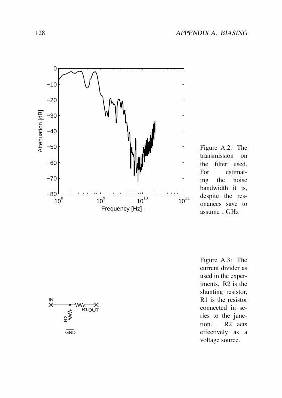
128 APPENDIX A. BIASING
108
109
1010
1011
−80
−70
−60
−50
−40
−30
−20
−10
0
Frequency [Hz]
Atte
nuat
ion
[dB
]
Figure A.2: Thetransmission onthe filter used.For estimat-ing the noisebandwidth it is,despite the res-onances save toassume 1 GHz
R2
R1
IN
OUT
GND
Figure A.3: Thecurrent divider asused in the exper-iments. R2 is theshunting resistor,R1 is the resistorconnected in se-ries to the junc-tion. R2 actseffectively as avoltage source.
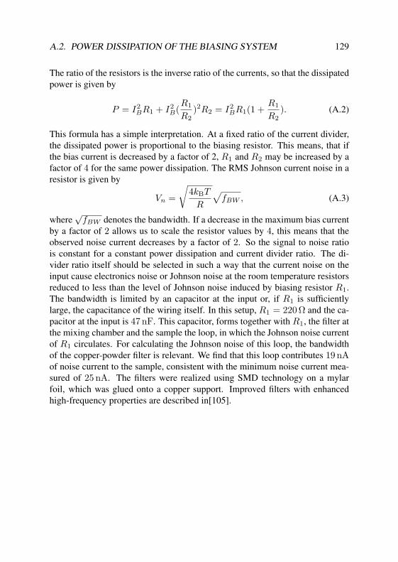
A.2. POWER DISSIPATION OF THE BIASING SYSTEM 129
The ratio of the resistors is the inverse ratio of the currents, so that the dissipatedpower is given by
P = I2BR1 + I2
B(R1
R2)2R2 = I2
BR1(1 +R1
R2). (A.2)
This formula has a simple interpretation. At a fixed ratio of the current divider,the dissipated power is proportional to the biasing resistor. This means, that ifthe bias current is decreased by a factor of 2, R1 and R2 may be increased by afactor of 4 for the same power dissipation. The RMS Johnson current noise in aresistor is given by
Vn =
√4kBT
R
√fBW , (A.3)
where√
fBW denotes the bandwidth. If a decrease in the maximum bias currentby a factor of 2 allows us to scale the resistor values by 4, this means that theobserved noise current decreases by a factor of 2. So the signal to noise ratiois constant for a constant power dissipation and current divider ratio. The di-vider ratio itself should be selected in such a way that the current noise on theinput cause electronics noise or Johnson noise at the room temperature resistorsreduced to less than the level of Johnson noise induced by biasing resistor R1.The bandwidth is limited by an capacitor at the input or, if R1 is sufficientlylarge, the capacitance of the wiring itself. In this setup, R1 = 220 Ω and the ca-pacitor at the input is 47 nF. This capacitor, forms together with R1, the filter atthe mixing chamber and the sample the loop, in which the Johnson noise currentof R1 circulates. For calculating the Johnson noise of this loop, the bandwidthof the copper-powder filter is relevant. We find that this loop contributes 19 nAof noise current to the sample, consistent with the minimum noise current mea-sured of 25 nA. The filters were realized using SMD technology on a mylarfoil, which was glued onto a copper support. Improved filters with enhancedhigh-frequency properties are described in[105].

130 APPENDIX A. BIASING

Appendix B
Electronics
B.1 Computer Control
All experiments are computer-controlled. Three different ways of interfacingthe measurement electronics with the computer are used in our setup. For char-acterization measurements, and for testing new pulse sequences like the shakerpreparation technique, National Instruments data acquisition cards[53] are used.These are capable of generating a timed triggered waveform output, and at thesame time perform buffered synchronized multi-channel data acquisition. TheRF-generator and the temperature controller are connected by an IEEE488-bus.In low-noise measurements serially interfaced 16-bit digital to analog DA con-verters [106] with galvanic isolation achieved by optical fibers [107]. Pulse-width modulation was used for the transfer of the digital data. Decoding to stan-dard serial programming interface (SPI) synchronous serial signals is done usingclockless logic [108]. Standard SPI daisy chaining is used share a single digitaltransmission channel for an arbitrary number of analog channels1. The temper-ature controller and the resistance measurement bridge are galvanically isolatedby an integrated optical fiber picobus interface[109]. The RF-generator outputis grounded to the shielding room feedthrough connector, but the rf ground andsignal are galvanically isolated by a DC break. The temperature controller isbattery powered like the analog electronics. A later test showed equivalent per-formance when using a properly filtered power supply unit.
1This is the functional description of the latest version of the DA, namely the triple DAmodule[108]. Earlier versions did not have the possibility of daisy chaining.
131

132 APPENDIX B. ELECTRONICS
B.2 Noise Estimation of the Ramp-Type Experi-ments
The resolution of the critical current measurements in ramp-type experiments islimited by several factors. The basic measurements involves current and voltage.Both are scaled, by either the monitor resistor in the current source or the voltagepreamplifier to a full-scale (−5 V . . . 5 V) signal for further signal processing.The noise of the voltage preamplifier and the current monitor amplifier are therelevant sources of noise at this point. In our standard measurement furthersignal processing consists of a trigger for each channel. This trigger is the onlynonlinear and hysteretic signal processing element. All white noise sources oneach channel can be summed up geometrically with the input noise of the trigger.At the trigger the analog input noise is translated into a timing error, known asjitter, which is proportional to the RMS input noise. The proportionality betweenthe jitter and the RMS noise value is given by the inverse slope of the input signalat the triggering point. Fig. B.1 illustrates the situation. This is equivalent to theusage of the error propagation formula for a single measured variable. We findthe relation of voltage noise to the jitter
σ(t) = σ(U)/U . (B.1)
A calculation of U is given below. The timing error itself translates to an errorin the detected switching current. For a constant slope of the current ramp, thetiming error is multiplied by the ramp rate:
σ(I) = σ(t)I . (B.2)
Thus we get a voltage signal processing path related current noise of
σ(I) =I
Uσ(U). (B.3)
It is obvious that if the voltage noise is the limitation on the current measur-ment precision, a change of the ramprate can remedy the problem at the costof longer measurment times. While a longer measurement time may be indesir-able, decreasing ramprate influences observable rates of escape. Since the rateof escape is directly related to the small oscillation frequency, a change in theramprate has the effect of shifting the measurement to another, non equivalent,bias point. On the signal path from the sample to the digital trigger output, dis-played in Fig. B.2, there are three elements which set the slew rate of the signal,

B.2. NOISE ESTIMATION OF THE RAMP-TYPE EXPERIMENTS 133
Utrig
U(t)Uin(t)
U(t)
σ(t)t
σ(U)
Figure B.1: A sketch of the error propagation of the voltage noise to the detectedtime of the switch. The red dash-dotted line represents the signal at the junction,while the black solid line represents the voltage at the trigger input. Projectingthe error in the voltage measurement onto the tangential of the voltage signalyields jitter.

134 APPENDIX B. ELECTRONICS
U_Trig
C+
R+ 2
16
V+ 7
V- 4
8
IC1
35
RG
C-
R-
GND
INA111P
GND GND
Figure B.2: The schematic of the total signal path from the Josephson junction(left) to the trigger (right). The input Utrig sets the threshold voltage.
or contribute to the noise. The resistors R+ and R− have a resistance of 1 kΩ.The Johnson noise voltage contribution from these resistors is negligible. TheRC time constant is measured to be 1/12 kHz, as measured. A voltage step ofV0 causes a maximum slope U at the time of the step, when the capacitor haszero voltage, so that V0 drives a current of I = V0/R through the resistor. Thisresults in a rate of voltage change across the capacitor of
U =1
RCV0. (B.4)
The preamplifier (INA111) contributes to the noise considerably. Its low-frequency noise contributes 1 µV peak to peak noise, and the white noise densityof ≈ 10 − 13 nV per
√Hz contributes up to ≈ 10 µV RMS noise at a gain of
1000 over the amplified band. The trigger has a input noise of 20 µV, whichcorresponds to 20 nV at the input of the amplifier. Putting in typical values forour setup 1
RC = 12 kHz, I = .02 A/s, and V0 = 2.5 mV, we find a voltageprocessing path related current noise of 8 nA. When detecting the jump to thevortex step V0 = 80µV, which would result in 250 nA of RMS noise,the outputbandwidth of this amplifier was limited to 20 kHz. For this value we find 35 nAof noise.
Estimating the noise of the current source, the relevant parts of which areschematized in Fig. B.3, is straightforward. Again the Johnson noise of themonitor resistor is negligible, due to the band selected by the RC-filters at the1 K-pot. Only the noise of the instrumentation amplifier monitoring the current

B.2. NOISE ESTIMATION OF THE RAMP-TYPE EXPERIMENTS 135
is relevant and the same as in the voltage path. Hence the noise is given by
σ(I) =σ(U)Rmon
, (B.5)
which yields approximately 10 nA for Rmon = 1kΩ. This noise is divided bythe cold current divider.

136 APPENDIX B. ELECTRONICS
V_in
2
16
V+7
V-4
8
IC1
35
R1
1
2
36
8
IC274
INA111P
OPA177P
GND
Figure B.3: The parts of the voltage controlled current source relevant for noisecalculations, including the monitor resistor R1, the feed-back loop on IC2, andthe instrumentation amplifier IC1.

Appendix C
Table of Samples andMeasurements
C.1 Samples Used
All samples investigated are manufactured using a tri-layer technology. In thistechnology, the junction barrier is not produced during the structuring unlikein the shadow evaporation technique. Instead a homogeneous bottom electrodefilm is grown on which a homogeneous barrier is formed, and a top electrode isdeposited. The advantages of this method are a high reproducibility and inde-pendence of the junction parameters and the structuring steps. Most of the inves-tigated samples, which are listed in table C.2, come from an external foundry,Hypres, which structures using photolithography. The design rules and restric-tions can be found in [66]. Only junction widths down to 3 µm are guarantiedby Hypres. However, a violation of the design rules yields working 2 µm widejunctions. For the sample SJJ-DAMP , the trilayer was produced by IPHT Jena,and the structuring was performed using e-beam lithography by Y. Koval. Thenominal trilayer critical current densities are listed in table C.1.
C.2 Table of Measurements
Table C.4 contains the measurements presented in this thesis. The measurementtype is either “Ensemble” (repeated measurement of IC as a function of parame-
137

138 APPENDIX C. TABLE OF SAMPLES AND MEASUREMENTS
Wafer Number Nominal critical current densityHypres KL700 30A/cm2
Hypres KL699 100A/cm2
Hypres KL698 1000A/cm2
Hypres KL519 1000A/cm2
Hypres KL366 100A/cm2
IPHT Jena, 200 A/cm2 200A/cm2
Table C.1: Trilayer identification, including the manufacturer. All trilayers pro-duced at Hypres are also structured there, while the trilayer provided at IPHTwas structured using e-beam lithography by Y. Koval.
Sample Wafer Width Radius (µm)AJJ-SHORT Hypres KL700 2 50AJJ-VAV IPHT Jena, 200 A/cm2 1 50AJJ-MS1 Hypres KL698 3 50AJJ-MS2 Hypres KL699 3 50AJJ-HEART1 Hypres KL519 3 50AJJ-HEART2 Hypres KL519 3 50AJJ-HEART3 Hypres KL519 3 50AJJ-INJ Hypres KL366 3 50SJJ-DAMP Hypres KL699 10x10 -
Table C.2: Dimensions of the junctions investigated. All samples besides SJJ-DAMP are topologically annular Josephson junctions, some which have a heart-shaped geometry or contain additional features, as listed in table C.3.
Sample Comments ChapterAJJ-SHORT Annular, Injectors 3,4AJJ-VAV E-beam lithography 4AJJ-MS1 Microshort 2 µm× 0.5 µm 5AJJ-MS2 Microshort 8 µm× 0.5 µm 3AJJ-HEART1 Heart β = 26o 5AJJ-HEART2 Heart β = 37o 5AJJ-HEART3 Heart β = 43o 5AJJ-INJ Injectors 2SJJ-DAMP Small junction 2
Table C.3: Details of the junctions investigated.

C.2. TABLE OF MEASUREMENTS 139
ters),“Spectroscopy” (Ensemble using RF-irradiation). The electronics are either“Tunnelelektronik-I” (TE-I) or “Tunnelelektronik-II” (TE-II), and can have thefollowing attributes: SR - shielded room; GND - ground-referenced signals inthe cryostat, CD - current dividers at 1K-pot, NIDAQ - waveform generationdirectly on the NIDAQ card; “NIDAQ - filtered” - waveform filtered by standardelectromagnetic interference suppression filters on the control signal. Commonto all measurements at temperatures below 4.2 K are copper-powder and highresistance coaxial line filters on the mixing chamber. All measurements not des-ignated by NIDAQ feature galvanic insulation of the analog electronics from thecomputer.

140 APPENDIX C. TABLE OF SAMPLES AND MEASUREMENTS
Sample Vorticity Measurementtype
Temp. [mK] Electronics
AJJ-SHORT 0 Ensemble(T, Hx) 28-400 TE-II (SR,GND, CD)
AJJ-SHORT 1I Ensemble(T, Hx) 28-400 TE-II (SR,GND, CD)
AJJ-INJ 1I, 1 IV, IC(H),IC(Hx, Hy)
4200 TE-I(NIDAQ)
AJJ-VAV 1 Ensemble(Hx, Hy),Spectr.1500 TE-I (SR)AJJ-VAV 0 Spectr. 28 TE-I (SR)AJJ-HEART1 1 IC(Hx, Hy),
IPC (Hx, Hy)
4200 TE-I(NIDAQ)
AJJ-HEART2 1 IC(Hx, Hy),IPC (Hx, Hy)
4200 TE-I(NIDAQ)
AJJ-HEART3 1 IC(Hx, Hy),IPC (Hx, Hy)
4200 TE-I(NIDAQ)
AJJ-MS2 1 Spectr. 150 TE-II (SR)AJJ-MS1 1 IC(Hy), bar-
rier suppression100-800,4200
TE-II (SR,GND, CD,NIDAQ-Filtered)
Table C.4: Measurements presented in this thesis.

Appendix D
Table of variables
Symbol Meaning Unit
Physical constantsΦ0 Magnetic flux quantum Vse Elementary charge Cµ0 Magnetic vacuum permeability N/A2
c Speed of light m/s
kB Boltzmann constant J/K
me Electron mass kg
Barrier propertiesC∗
j Specific (junction) capacitance F/m2
R∗ Specific resistance Ωm2
∆G Superconducting gap eVL∗ Inductance per square Hjc Critical current density A/m2
λJ Josephson length mλL London penetration depth md′ Magnetic thickness mtJ Barrier thickness mωP Plasma frequency Hzc Swihart velocity m/s
141

142 APPENDIX D. TABLE OF VARIABLES
Symbol Meaning UnitH0 Field normalization constant G
Junction propertiesEJ Josephson energy JIC Critical current ACj Junction capacitance FRj Quasiparticle resistance ΩR0 Ohmic resistance Ω
Experimental paramters and observablesν AC Josephson frequency HzΓesc Decay rate HzΓesc,rf Decay rate in presence of rf HzΓqu Quantum decay rate HzΓth Thermal decay rate HzT ∗ Crossover temperature KT Temperature K~Hext External magnetic field GHext External magnetic field amplitude GHext,cr External critical magnetic field am-
plitudeG
hext,cr External critical magnetic field am-plitude
norm.
Ib Bias current AIn RMS of Johnson/Nyquist noise cur-
rentA
IPC Critical current, determined after
state preparationA
Iinj Injected current AΦext External magnetic flux VsV Voltage VV0 Vortex step voltage V~jinp In plane supercurrent density A/m
ω0 Small oscillation frequency norm.
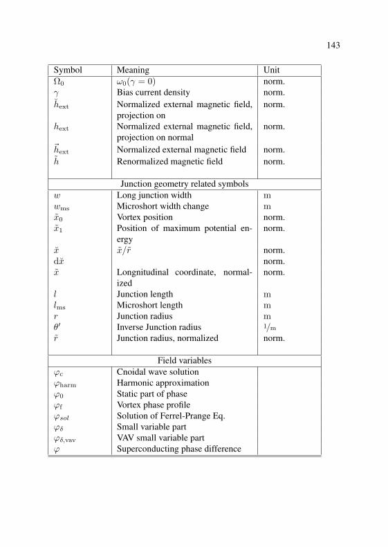
143
Symbol Meaning UnitΩ0 ω0(γ = 0) norm.γ Bias current density norm.hext Normalized external magnetic field,
projection onnorm.
hext Normalized external magnetic field,projection on normal
norm.
~hext Normalized external magnetic field norm.h Renormalized magnetic field norm.
Junction geometry related symbolsw Long junction width mwms Microshort width change mx0 Vortex position norm.x1 Position of maximum potential en-
ergynorm.
x x/r norm.dx norm.x Longnitudinal coordinate, normal-
izednorm.
l Junction length mlms Microshort length mr Junction radius mθ′ Inverse Junction radius 1/m
r Junction radius, normalized norm.
Field variablesϕc Cnoidal wave solutionϕharm Harmonic approximationϕ0 Static part of phaseϕf Vortex phase profileϕsol Solution of Ferrel-Prange Eq.ϕδ Small variable partϕδ,vav VAV small variable partϕ Superconducting phase difference
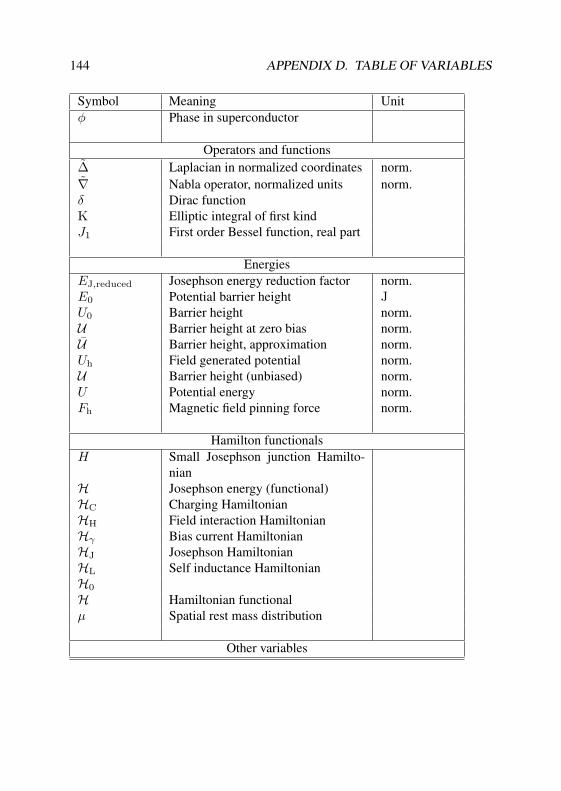
144 APPENDIX D. TABLE OF VARIABLES
Symbol Meaning Unitφ Phase in superconductor
Operators and functions∆ Laplacian in normalized coordinates norm.∇ Nabla operator, normalized units norm.δ Dirac functionK Elliptic integral of first kindJ1 First order Bessel function, real part
EnergiesEJ,reduced Josephson energy reduction factor norm.E0 Potential barrier height JU0 Barrier height norm.U Barrier height at zero bias norm.U Barrier height, approximation norm.Uh Field generated potential norm.U Barrier height (unbiased) norm.U Potential energy norm.Fh Magnetic field pinning force norm.
Hamilton functionalsH Small Josephson junction Hamilto-
nianH Josephson energy (functional)HC Charging HamiltonianHH Field interaction HamiltonianHγ Bias current HamiltonianHJ Josephson HamiltonianHL Self inductance HamiltonianH0
H Hamiltonian functionalµ Spatial rest mass distribution
Other variables
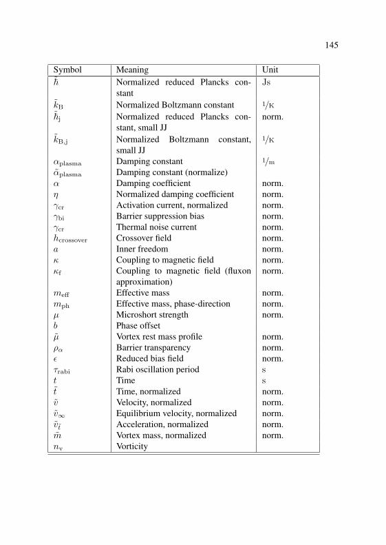
145
Symbol Meaning Unit~ Normalized reduced Plancks con-
stantJs
kB Normalized Boltzmann constant 1/K
~j Normalized reduced Plancks con-stant, small JJ
norm.
kB,j Normalized Boltzmann constant,small JJ
1/K
αplasma Damping constant 1/m
αplasma Damping constant (normalize)α Damping coefficient norm.η Normalized damping coefficient norm.γcr Activation current, normalized norm.γbi Barrier suppression bias norm.γcr Thermal noise current norm.hcrossover Crossover field norm.a Inner freedom norm.κ Coupling to magnetic field norm.κf Coupling to magnetic field (fluxon
approximation)norm.
meff Effective mass norm.mph Effective mass, phase-direction norm.µ Microshort strength norm.b Phase offsetµ Vortex rest mass profile norm.ρα Barrier transparency norm.ε Reduced bias field norm.τrabi Rabi oscillation period st Time st Time, normalized norm.v Velocity, normalized norm.v∞ Equilibrium velocity, normalized norm.vt Acceleration, normalized norm.m Vortex mass, normalized norm.nv Vorticity

146 APPENDIX D. TABLE OF VARIABLES
Symbol Meaning UnitAqu KFD quantum prefactorAth KFD thermal prefactorBqu KFD quantum exponentBth KFD thermal exponentA KFD prefactorA Arrhenius factorB KFD exponentSb Barrier action, see [62]S0 Barrier action at zero bias, see [62]q Reaction coordinateHs Magnetic field in superconductorχ Small amplitide nucleus sizeωB Unstable barrier frequencyU Signal slew rate, input referredσ(U) Signal rms noise, input referredσ(t) JitterI Current ramp rateσ(t) Current noise

Bibliography
[1] B. D. Josephson, Phys. Lett. 1, 251 (1962).
[2] A. J. Dahm, A. Denenstein, D. N. Langenberg, W. H. Parker, D. Rogovin,and D. J. Scalapino, Phys. Rev. Lett. 22, 1416 (1969).
[3] T. Fulton and L. Dunkelberger, Phys. Rev. B 9, 4760 (1974).
[4] J. Kurkijarvi, Phys. Rev. B 6, 832 (1972).
[5] R. Voss and R. A. Webb, Phys. Rev. Lett. 47, 265 (1981).
[6] M. Devoret, J. Martinis, and J. Clarke, Phys. Rev. Lett. 55, 1908 (1985).
[7] J. Martinis, M. Devoret, and J. Clarke, Phys. Rev. B 35, 4682 (1987).
[8] A. Wallraff, Fluxon Dynamics in annular Josephson juctions: From rela-tivistic strings to quantum particles, Ph.D. thesis, University of Erlangen-Nurnberg, Germany (2000).
[9] A. Wallraff, A. Lukashenko, J. Lisenfeld, A. Kemp, M. Fistul, Y. Koval,and A. V. Ustinov, Nature 425, 155 (2003).
[10] A. Kemp, Fluxon states in heart-shaped Josephson Junctions, Master’sthesis, FAU Erlangen-Nurnberg (2001).
[11] A. Kemp, A. Wallraff, and A. V. Ustinov, Physica C 368, 324 (2002).
[12] A. Kemp, A. Wallraff, and A. V. Ustinov, Phys. stat. sol. 233, 472 (2002).
[13] A. Wallraff, Y. Koval, M. Levitchev, M. V. Fistul, and A. V. Ustinov, J.Low Temp. Phys. 118, 543 (2000).
147
148 BIBLIOGRAPHY
[14] M. Castellano, G. Torrioli, C. Cosmelli, A. Costantini, F. Chiarello,P. Carelli, G. Rotoli, M. Cirillo, and R. Kautz, Phys. Rev B 54, 15417(1996).
[15] D. Gulevich and F. Kusmartsev, Physica C 435, 87 (2006).
[16] M. Fistul, A. Wallraff, Y. Koval, A. Lukashenko, B. A. Malomed, andA. V. Ustinov, Phys. Rev. Lett. 91, 257004 (2003).
[17] C. Gorria, Y. B. Gaididei, M. P. Soerensen, P. L. Christiansen, and J. G.Caputo, Phys. Rev. B 69, 134506, 134506 (10 pages) (2004).
[18] P. Shaju and V. Kuriakose, Phys. Lett. A 332, 326 (2004).
[19] E. Goldobin, A.Sterk, and D. Koelle, Phys. Rev. E 63 (2001).
[20] A. Kemp, A. Price, and A. V. Ustinov, Unpublished pp. – (2006).
[21] A. Price, A. Kemp, and A. V. Ustinov, In preparation pp. – (2006).
[22] J. Bardeen, L. Cooper, and J. Schrieffer, Phys. Rev. B 108, 1175 (1957).
[23] J. S. Langer and V. Ambegaokar, Phys. Rev. 164, 498 (1967).
[24] A. G. Sivakov, A. M. Glukhov, A. N. Omelyanchouk, Y. Koval, P. Muller,and A. V. Ustinov, Phys. Rev. Lett. 91, 267001, 267001 (4 pages) (2003).
[25] A. A. Abrikosov, Sov. Phys. JETP 5, 1174 (1957).
[26] L. V. Shubnikov and al, Zh. Eksp. Teor. Fiz 7, 221 (1937).
[27] J. Anderson and J. Rowell, Phys. Rev. Lett. 10, 230 (1963).
[28] V. Ambegaokar and A. Baratoff, Phys. Rev. Lett. 10, 486 (1963).
[29] M. Tinkham, Introduction to Superconductivity (McGraw-Hill Interna-tional Editions, 1996).
[30] V. Ambegaokar, U. Eckern, and G. Schon, Phys. Rev. Lett. 48, 1745(1982).
[31] T. Sheahen, Phys. Rev. 149, 368 (1966).
[32] J. Johnson, Phys. Rev. 32, 97 (1928).
[33] H. Nyquist, Phys. Rev. 32, 110 (1928).

BIBLIOGRAPHY 149
[34] W. Schottky, Annalen der Physik 23, 541 (1918).
[35] A. V. Ustinov, Physica D 123, 315 (1998).
[36] A. V. Ustinov, Solitons in Josephson Junctions : Physics of MagneticFluxons in Superconducting Junctions and Arrays (Hardcover) (John Wi-ley & Sons, 2005).
[37] N. Pedersen, Advances in Superconductivity (Plenum Press, New York,1982), chap. Solitons in long Josephson junctions.
[38] R. Parmentier, The new superconducting electronics (Kluwer, Dordrecht,1993), p. 221.
[39] R. Peierls, Proc. of the Phys. Soc. 52, 34 (Jan. 1940).
[40] J. D. Jackson, Classical electrodynamics (Wiley, New York, 1962), sec-ond edition ed., third edition does not contain plasma physics.
[41] V. S. Kaplunenko and A. V. Ustinov, Long Josephson junctions as filters:stopband calculation, personal communation.
[42] G. Lee and A. Barfknecht, IEEE Trans. Appl. Supercond. 2, 67 (1992).
[43] J. Caputo, N. Flytzanis, and M. Devoret, Phys. Rev. B 50, 6471 (1004).
[44] A. Franz, A. Wallraff, and A. V. Ustinov, J. Appl. Phys. 89, 471 (2001).
[45] A. Ustinov, APL 80, 3153 (2002).
[46] M. Cirillo, R. Parmentier, and B. Savo, Physica 3D 18, 565 (1981).
[47] D. McLaughlin and A. Scott, Phys. Rev. A 18, 1652 (1978).
[48] N. Grønbech-Jensen, P. Lomdahl, and M. Samuelsen, Phys. Lett. A 154,14 (1991).
[49] T. Fliessbach, Mechanik (Elsevier, 2003), 4th ed.
[50] N. F. Pedersen and D. Welner, Phys. Rev. B 29, 2551 (1984).
[51] National Instruments, PCI E Series User Manual.
[52] National Instruments, NI-DAQ Function Reference Manual for PC Com-patibles.
150 BIBLIOGRAPHY
[53] National Instruments, NI-DAQ User Manual for PC Compatibles.
[54] Stanford Research Systems, SR 620 universal time interval counter.
[55] A. Wallraff, A. Lukashenko, C. Coqui, A. Kemp, T. Duty, and A. V. Usti-nov, Rev. of Sci. Instr. 74, 3740 (2003).
[56] B. A. Malomed and A. V. Ustinov, Phys. Rev. B 69, 064502, 064502 (8pages) (2004).
[57] P. Silvestrini, V. Palmieri, B. Ruggiero, and M. Russo, Phys. Rev. Lett.79, 3046 (1997).
[58] P. Silvestrini, O. Liengme, and K. E. Gray, Phys. Rev. B 37, 1525 (1988).
[59] R. A. Fisher, Messenger of Math. 41, 155 (1912).
[60] A. Garg, Phys. Rev. B 51, 15592 (1995).
[61] H. Kramers, Physica 7, 284 (1940).
[62] M. Buttiker, E. Harris, and R. Landauer, Phys. Rev. B 28, 1268 (1983).
[63] M. Fistul, A.Wallraff, Y. Koval, A. Lukashenko, B. A. Malomed, andA. V. Ustinov, Phys. Rev. Lett. 93, 257004 (2003).
[64] D. Esteve, M. H. Devoret, and J. M. Martinis, Phys. Rev. B 34, 158(1986).
[65] A. Davidson, B. Dueholm, B. Kryger, and N. Pedersen, Phys. Rev. Lett.55, 2059 (1985).
[66] S. K. Tolpygo, elmsford, NY 10523, U.S.A.
[67] A. A. Golubov, B. A. Malomed, and A. V. Ustinov, Phys. Rev. B 54, 3047(1996).
[68] B. A. Malomed and A. Ustinov, Phys. Lett. p. 284 (1989).
[69] Y. Kivshar and B. Malomed, Rev. Mod. Phys. 61, 763 (1989).
[70] M. H. Devoret, D. Esteve, J. M. Martinis, A. Cleland, and J. Clarke, Phys.Rev. B 36, 58 (1987).

BIBLIOGRAPHY 151
[71] N. Grønbech-Jensen, M. Castellano, F. Chiarello, M. Cirillo, C. Cosmelli,L. Filippenko, R. Russo, and G. Torrioli, Phys. Rev. Lett. 93, 107002(2004).
[72] P. Jung and P. Hanggi, Phys. Rev. A 41, 2977 (March 1990).
[73] P. Hanggi, F. Marchesoni, and P. Riseborough, Europhysics Letters 13,223 (1990).
[74] R. Simmonds, K. Lang, D. A. Hite, S. Nam, D. P. Pappas, and J. M.Martinis, Phys. Rev. Lett. 93, 077003 (2004).
[75] J. M. Martinis, K. B. Cooper, R. McDermott, M. Steffen, M. Ansmann,K. D. Osborn, K. Cicak, S. Oh, D. P. Pappas, R. Simmonds, et al., Phys.Rev. Lett. 95, 210503 (2005).
[76] M. von Schickfus and S. Hunklinger, Phys. Lett. 64A, 144 (1977).
[77] B. Golding, M. v. Schickfus, S. Hunklinger, and K. Dransfeld, Phys. Rev.Lett. 43, 1817 (1979).
[78] P. Hanggi, P. Talkner, and M. Borkovec, Rev. Mod. Phys. 62, 251 (1990).
[79] U. Weiss, Quantum dissipative systems (World Scientific, 1999), 2nd ed.
[80] M. V. Fistul, V. M. Vinokur, A. Kemp, and A. V. Ustinov, unpub. pp. –(2006).
[81] A. Shnirman, E. Ben-Jacob, and B. Malomed, Phys. Rev. B 56, 14677(1997).
[82] T. Kato and M. Imada, J. Phys. Soc. Jpn. 65, 2963 (1996).
[83] P. Hanggi, Z. Physik B 68, 181 (1987).
[84] M. Buttiker and R. Landauer, Phys. Rev. A 23, 1397 (1981).
[85] P. Hanggi, F. Marchesoni, and P. Sodano, Phys. Rev. Lett. 60, 2563(1988).
[86] K. Hida and U. Eckern, Phys. Rev. B 30, 4096 (1984).
[87] B. I. Ivlev and Y. N. Ovchinnikov, Sov. Phys. JETP 66, 378 (1987).
[88] T. Kato, J. of the Phys. Society of Japan 69, 2735 (September 2000).

152 BIBLIOGRAPHY
[89] T. Kato, Phys. Rev. B p. submitted (2001), fig. 5.: Crossover length.
[90] C. Nappi, Phys. Rev. B 55, 82 (1997).
[91] N. Martucciello and R. Monaco, Phys. Rev. B 54, 9050 (1996).
[92] N. Martucciello, R. Monaco, and C. Soriano, Annular Josephson tunneljunctions in external magnetic field, (preprint).
[93] A. Franz, A. Wallraff, and A. V. Ustinov, Phys. Rev. B 62, 119 (2000).
[94] A. Kemp, M. Fistul, A. Wallraff, Y. Koval, A. Lukashenko, B. Mal-omed, and A. Ustinov, in B. Ruggiero, P. Delsing, C. Granata, Y. Pashkin,and P. Silvestrini, eds., Quantum Computation in Solid State Systems(Springer, Heidelberg, 2006).
[95] A. J. Leggett, S. Chakravarty, A. T. Dorsey, M. P. A. Fisher, A. Garg, andW. Zwerger, Rev. Mod. Phys. 59, 1 (1987).
[96] A. Shnirman, G. Schon, and Z. Hermon, Phys. Rev. Lett 79, 2371 (1997).
[97] J. H. Kim and R. P. Dhungana, to appear in Phys. Rev. B (2006), cond-mat/0604431.
[98] D. Gulevich, A. Kemp, A. Price, A. V. Ustinov, and F. Kusmartsev, un-published (2006).
[99] A. Ustinov, B. A. Malomed, and N. Thyssen, Phys. Lett. A 233, 239(1997).
[100] I. Serpuchenko and A. Ustinov, JETP Lett. 46, 435 (1987).
[101] V. Oboznov and A. V. Ustinov, Phys. Lett. A 139, 481 (1989).
[102] Wolfram Research Inc., Mathematica.
[103] A. Price, personal communication.
[104] S. K. Tolpygo, Design rules (2005), process #100-1000-2500-1, Revision22.
[105] D. Freitag and C. Gluth, SMD Filters, Lab course report, PI3, FAU (2006).
[106] Texas Instruments, DAC714 datasheet.

BIBLIOGRAPHY 153
[107] Agilent Technologies, HG2410 fiber optics transmission set.
[108] F. Schmitt, Beschreibung zu Glasfaser-Ubertragungsmodul.
[109] Picowatt, AVS47 II-B Manual.
[110] E. Goldobin, e. Goldobin, Goldexi,http://www.geocities.com/SiliconValley/Heights/7318/.
[111] M. Devoret, J. M. Martinis, D. Esteve, and J. Clarke, Phys. Rev. Lett. 53,1260 (1984).

154 BIBLIOGRAPHY

Acknowledgements
To Prof. Alexey Ustinov for giving me the opportunity to discover interestingphysics at a variety of interesting systems. To Prof. Paul Muller I thank for hisefforts to keep this institute a working and interesting place for research.
The group which was allowed to work in allowed me to gather inter-culturalexperiences, which I am sure I will profit from for the rest of my life. It isimpossible to mention all people who made my stay here interesting; yet therewere a few which contributed more to my work than others. Especially I have tothank to
• Astria Price for support of the measurements on shaped junctions and themicroshort junctions. She also proofread this thesis to make the Englishmore bearable.
• Dmitry Gulevich and Prof. Feodor Kusmartsev for efficient collaboration.
• Christian Coqui for invaluable help by the construction of the newshielded room and lot of electronics development and beeing a very nicecolleague.
• Dr. Andreas Wallraff for beeing the co-initiator, together with Prof. Usti-nov of the vortex qubit project; and sharing, while beeing the supervisorof my diploma thesis some important skills, which i am lacking.
• Dr. Koval for his patience and the production of samples.
• Dr. Kaplunenko for teaching me important things about RSFQ logics andprofessional software development.
• Hans Eglmeier for discussions on symmetry, logics and everything andfor using his incredible mechanical construction talent in our group.
155

156 ACKNOWLEDGEMENTS
• Prof. Hanggi for pointing out important references, which help me a lot inunderstanding the topic of soliton pair nucleation.
• Tobias Wirth for discussions on electronics and other interesting things.
• Dr. Abdufarrukh A. Abdumalikov for being very often complementary tomy “hand-waving” approach of physics - and by that teaching me some-times more than he probably suspects himself.
• Judith Pfeiffer for being a nice colleague.
• Dr. Goldobin for the interesting exchange of ideas.
• Dr. Lukashenko for sharing some of his profound low temperature engi-neering knowledge.
• Jurgen Lisenfeld for sharing parts of GPIB driver modules.
• The DAAD for funding a language course and PTU Tomsk for hospitality.
• The DAAD for funding a research visit and Prof. Ryazanov and his groupfor hospitality and introducing me to SQUID picovoltmeters.
• The DFG for funding in terms of the focused research program “Quanten-informationsverarbeitung”.
• NTT for hospitality during a summer school.
• Dr. Tim Duty for showing me MATLAB as a data acquisition system.
• The IPHT Jena, especially Dr. Kunert for the fabrication of samples.
• Prof. Fistul for theoretical support.
• Prof. Ken Matsuda for help in experiments during his visit.
• The members of the “Haustechnik”, which keep the institute building run-ning very well and helped me on everything I needed.
• The electronic workshop, especially Mr. Gretzbach, who is the main main-tainer and developers of the analog electronics.
• The mechanical workshop, where I could not only give the plans, but dis-cuss them, too.
156

ACKNOWLEDGEMENTS 157
• Our secretary, Mrs. Metze for the valuable work she does everyday; espe-cially for help in the fight against forms.
My personal acknowledgements go to
• My flatmates Anne, Caroline and Rhea for being an important balance inmy life.
• Alexander Grujic, Helmut Holzler, Tobias Kampfrath and Alexandra We-ichlein for discussions about physics and beeing friends.
• My father for supporting my studies.
157

158 ACKNOWLEDGEMENTS
158
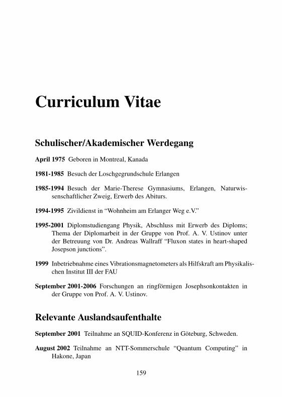
Curriculum Vitae
Schulischer/Akademischer WerdegangApril 1975 Geboren in Montreal, Kanada
1981-1985 Besuch der Loschgegrundschule Erlangen
1985-1994 Besuch der Marie-Therese Gymnasiums, Erlangen, Naturwis-senschaftlicher Zweig, Erwerb des Abiturs.
1994-1995 Zivildienst in “Wohnheim am Erlanger Weg e.V.”
1995-2001 Diplomstudiengang Physik, Abschluss mit Erwerb des Diploms;Thema der Diplomarbeit in der Gruppe von Prof. A. V. Ustinov unterder Betreuung von Dr. Andreas Wallraff “Fluxon states in heart-shapedJosepson junctions”.
1999 Inbetriebnahme eines Vibrationsmagnetometers als Hilfskraft am Physikalis-chen Institut III der FAU
September 2001-2006 Forschungen an ringformigen Josephsonkontakten inder Gruppe von Prof. A. V. Ustinov.
Relevante AuslandsaufenthalteSeptember 2001 Teilnahme an SQUID-Konferenz in Goteburg, Schweden.
August 2002 Teilnahme an NTT-Sommerschule “Quantum Computing” inHakone, Japan
159

160 CURRICULUM VITAE
September 2003-Oktober 2003 Forschungsaufenthalt im Rahmen eines DAAD-Stipendiums am Festkorperforschungsinstitut in Chernogolovka, Russ-land
Sonstige Konferenzbeitrage• DPG Fruhjahrstagung 2001, 2003, 2004, 2005, 2006 (Poster)
• Kryo Konferenz 2000, Intrinsic Konferenz 2002
• DFG QIV SPP Seminar 2002, 2004, 2005
160