Quantum Algorithmic Techniques for Fault-Tolerant Quantum ...
182
Quantum Algorithmic Techniques for Fault-Tolerant Quantum Computers by M´ aria Kieferov´ a A thesis presented to the University of Waterloo in fulfillment of the thesis requirement for the degree of Doctor of Philosophy in Physics (Quantum Information) Waterloo, Ontario, Canada, 2019 c M´ aria Kieferov´ a 2019
Transcript of Quantum Algorithmic Techniques for Fault-Tolerant Quantum ...

Quantum Algorithmic Techniquesfor Fault-Tolerant Quantum
Computers
by
Maria Kieferova
A thesispresented to the University of Waterloo
in fulfillment of thethesis requirement for the degree of
Doctor of Philosophyin
Physics (Quantum Information)
Waterloo, Ontario, Canada, 2019
c©Maria Kieferova 2019

Supervisor: Michele Mosca, Professor,Dept. of Combinatorics & Optimization,University of Waterloo
Supervisor (cotutelle): Dominic Berry, Assoc. Professor,Dept. of Physics & Astronomy,Macquarie University
Committee Member: Christine Muschik, Assist. Professor,Dept. of Physics & Astronomy,University of Waterloo
Committee Member: Daniel Gottesman, Professor,Dept. of Physics & Astronomy,(Perimeter Institute) University of Waterloo
Internal-External Examiner: Ashwin Nayak, Professor,Dept. of Combinatorics & Optimization,University of Waterloo
External Examiner: Ashley Montanaro, Reader,School of Mathematics,University of Bristol
ii

Author’s Declaration
This thesis is being submitted to Macquarie University and the Universityof Waterloo in accordance with the Cotutelle agreement dated February 10,2017.
This thesis consists of material all of which I authored or co-authored: seeStatement of Contributions included in the thesis.
I understand that my thesis may be made electronically available to thepublic.
Maria Kieferova
iii

Statement of Contributions
Chapter 1MK wrote this chapter as an introduction to the thesis.
Chapter 2Section 2.3 is based on part 4.1 of my publication [1] but has been extendedto cover Hamiltonian simulation techniques in more detail. The rest of thechapter was written by MK solely for this thesis.
• MK wrote the majority of Chapter 4 of [1] with inputs and revisionsfrom other authors, in particular Peter Johnson, Yudong Cao and IanKivlichan.
Chapter 3Chapter 3 is based on [2]. This chapter was edited and Sections 3.1 and 3.5added for completeness.
The project was proposed by Dominic Berry and Ryan Babbush.
• MK contributed to the antisymmetrization procedure in [2] with ideasand writing.• MK designed the parallelized quantum comparator with inputs from
Artur Scherer, Dominic Berry and Craig Gidney.
Chapter 4Chapter 4 is based on the publication [3]. This chapter was edited, andFig. 4.1 added for clarity.
The project was proposed by Dominic Berry.
• MK contributed to all parts of the project.• MK wrote the majority of the paper together with Artur Scherer and
Dominic Berry.
iv

Chapter 5Chapter 5 is based on [4]. This chapter was extensively edited, updatedfor new developments, and an introduction to Boltzmann machines wasadded. We also added multiple figures for clarity.
The project was proposed by Nathan Wiebe.
• MK contributed with ideas for defining a quantum training set.• MK contributed to the development of POVM and relative entropy
training.• MK performed the simulations in Sections 5.6.3 and 5.6.4 and the
comparison between Golden-Thompson and relative entropy trainingin 5.6.5.• MK proved Theorem 8.• MK contributed to the writing of the paper.
Chapter 7MK wrote this chapter as a conclusion for this thesis.
Appendix AMK wrote this appendix to provide additional background information forChapter 5.
v
Abstract
Quantum computers have the potential to push the limits of computationin areas such as quantum chemistry, cryptography, optimization, and ma-chine learning. Even though many quantum algorithms show asymptoticimprovement compared to classical ones, the overhead of running quan-tum computers limits when quantum computing becomes useful. Thus, byoptimizing components of quantum algorithms, we can bring the regimeof quantum advantage closer. My work focuses on developing efficientsubroutines for quantum computation. I focus specifically on algorithmsfor scalable, fault-tolerant quantum computers. While it is possible thateven noisy quantum computers can outperform classical ones for specifictasks, high-depth and therefore fault-tolerance is likely required for mostapplications. In this thesis, I introduce three sets of techniques that can beused by themselves or as subroutines in other algorithms.
The first components are coherent versions of classical sort and shuffle.We require that a quantum shuffle prepares a uniform superposition overall permutations of a sequence. The quantum sort is used within the shuffleand as well as in the next algorithm in this thesis. The quantum shuffle isan essential part of state preparation for quantum chemistry computationin first quantization.
Second, I review the progress of Hamiltonian simulations and give anew algorithm for simulating time-dependent Hamiltonians. This algo-rithm scales polylogarithmic in the inverse error, and the query complexitydoes not depend on the derivatives of the Hamiltonian. A time-dependentHamiltonian simulation was recently used for interaction picture simula-tion with applications to quantum chemistry.
Next, I present a fully quantum Boltzmann machine. I show that ouralgorithm can train on quantum data and learn a classical description of
vi

quantum states. This type of machine learning can be used for tomography,Hamiltonian learning, and approximate quantum cloning.
vii

Acknowledgement
This thesis would not be possible without a number of people supportingme throughout my PhD studies. I would first like to thank my supervisorsMichele Mosca, Dominic Berry and Gavin Brennen for all their time, adviceand encouragement. I cannot thank Michele enough for his guidance sincemy first internship at IQC in 2012. I would also like to thank Dominic foreverything I learned from him and his many comments on earlier drafts ofthis thesis.
I am very grateful to my advisory committee consisting of Daniel Gottes-man, Ashwin Nayak, and Roger Melko as well as additional examinersChristine Muschik, Ashley Montanaro, David Poulin and Jingbo Wang fortaking the time to read my thesis and for their helpful suggestions.
I want to thank Microsoft Research and Zapata Computing for givingme the opportunities to join them as an intern during my studies. Spendingtime in a corporate environment enriched my academic experience, and Ithoroughly enjoyed both of my internships.
I would also like to thank everyone involved in the FKS competitionfor opening the doors of physics for me, my former supervisor DanielNagaj for introducing me to quantum computing and Nathan Wiebe forhis ongoing mentorship. I am also thankful to my friends and colleaguesfor all the conversations that enriched me academically.
I would not be able to carry out the research in this thesis withoutmy collaborators Ryan Babbush, Yudong Cao, Matthias Degroote, CraigGidney, Peter D Johnson, Alan Aspuru-Guzik, Ian D Kivlichan, Guang HaoLow, Tim Menke, Jonathan Olson, Borja Peropadre, Sadegh Raeisi, JonathanRomero, Nicolas PD Sawaya, Sukin Sim, Yuval Sanders, Artur Scherer andLibor Veis. I thank Mike and Ophelia Lazaridis Fellowship, University ofWaterloo, Michele Mosca and Macquarie University for financial support.
viii

Lastly, I want to thank my parents for raising me, to Danielka for herfriendship since the day she was born and to Yuval for his love and caffeinesupply.
ix

Table of Contents
List of Figures xiv
List of Abbreviations xv
1 Introduction 1
1.1 Quantum Computing Hardware in 2019 . . . . . . . . . . . . 2
1.2 Quantum Computing Software in 2019 . . . . . . . . . . . . . 4
1.3 Overview . . . . . . . . . . . . . . . . . . . . . . . . . . . . . . 5
1.4 Notation . . . . . . . . . . . . . . . . . . . . . . . . . . . . . . 6
2 Background 8
2.1 Preliminaries . . . . . . . . . . . . . . . . . . . . . . . . . . . . 9
2.1.1 Quantum Gates and the Circuit Model . . . . . . . . 9
2.1.2 Complexity . . . . . . . . . . . . . . . . . . . . . . . . 11
2.1.3 Error Correction and the Threshold Theorem . . . . . 12
2.2 A Brief Overview of Quantum Algorithms . . . . . . . . . . 14
2.2.1 Coherent Classical Computation . . . . . . . . . . . . 15
2.2.2 Phase Estimation and Eigenstate Preparation . . . . . 16
2.2.3 Grover Search and Amplitude Amplification . . . . . 19
2.2.4 Oblivious Amplitude Amplification . . . . . . . . . . 22
2.3 Hamiltonian Evolution Simulation . . . . . . . . . . . . . . . 22
x

2.3.1 The Hamiltonian Oracles . . . . . . . . . . . . . . . . 24
2.3.2 Lower Bounds on Hamiltonian Simulation . . . . . . 26
2.3.3 Simulation Based on Trotterization . . . . . . . . . . . 28
2.3.4 Sparse Matrix Decomposition . . . . . . . . . . . . . . 29
2.3.5 The Quantum Walk Approach . . . . . . . . . . . . . 31
2.3.6 Hamiltonian Simulation with Linear Combination ofUnitaries . . . . . . . . . . . . . . . . . . . . . . . . . . 34
2.3.7 Quantum Signal Processing and Qubitization . . . . 36
2.3.8 Generalization of the Hamiltonian Simulation Problem 38
3 Quantum Sort and Shuffle 40
3.1 How to Shuffle a Deck of Cards . . . . . . . . . . . . . . . . . 41
3.2 Quantum Approach to a Shuffle . . . . . . . . . . . . . . . . . 43
3.3 Preparing a Uniform Superposition With the Quantum FYShuffle . . . . . . . . . . . . . . . . . . . . . . . . . . . . . . . 44
3.3.1 Initialization . . . . . . . . . . . . . . . . . . . . . . . . 47
3.3.2 FY Blocks . . . . . . . . . . . . . . . . . . . . . . . . . 48
3.3.3 Disentangling index from input . . . . . . . . . . . . 51
3.3.4 Complexity Analysis of the FY shuffle . . . . . . . . . 52
3.4 Symmetrization Through Quantum Sorting . . . . . . . . . . 53
3.4.1 Quantum Sorting Network . . . . . . . . . . . . . . . 55
3.4.2 Quantum Comparator . . . . . . . . . . . . . . . . . . 59
3.4.3 Analysis of ‘Delete Collisions’ Step . . . . . . . . . . . 65
3.4.4 Complexity Analysis of the Shuffle via Sorting . . . . 67
3.5 Applications . . . . . . . . . . . . . . . . . . . . . . . . . . . . 68
3.6 Conclusion . . . . . . . . . . . . . . . . . . . . . . . . . . . . . 70
xi

4 Simulation of Time-Dependent Hamiltonians 71
4.1 Unitary Evolution Under a Time-dependentHamiltonian . . . . . . . . . . . . . . . . . . . . . . . . . . . . 72
4.2 Framework . . . . . . . . . . . . . . . . . . . . . . . . . . . . . 73
4.2.1 Oracles . . . . . . . . . . . . . . . . . . . . . . . . . . . 73
4.2.2 Enabling Oblivious Amplitude Amplification . . . . 75
4.3 Algorithm Overview . . . . . . . . . . . . . . . . . . . . . . . 77
4.3.1 Evolution Discretization . . . . . . . . . . . . . . . . . 77
4.3.2 Linear Combination of Unitaries . . . . . . . . . . . . 81
4.4 Preparation of Auxiliary Registers . . . . . . . . . . . . . . . 84
4.4.1 Clock Preparation Using Compressed Rotation En-coding . . . . . . . . . . . . . . . . . . . . . . . . . . . 86
4.4.2 Clock Preparation Using a Quantum Sort . . . . . . . 88
4.4.3 Completing the State Preparation . . . . . . . . . . . 90
4.5 Complexity Requirements . . . . . . . . . . . . . . . . . . . . 95
4.5.1 Complexity for Scenario 1 . . . . . . . . . . . . . . . . 96
4.5.2 Complexity for Scenario 2 . . . . . . . . . . . . . . . . 98
4.6 Results . . . . . . . . . . . . . . . . . . . . . . . . . . . . . . . 99
4.7 Applications . . . . . . . . . . . . . . . . . . . . . . . . . . . . 100
4.8 Conclusion . . . . . . . . . . . . . . . . . . . . . . . . . . . . . 102
5 Training and Tomography with Quantum Boltzmann Machines 103
5.1 Quantum Machine Learning . . . . . . . . . . . . . . . . . . . 104
5.2 Boltzmann Machines . . . . . . . . . . . . . . . . . . . . . . . 105
5.3 Training Quantum Boltzmann Machines . . . . . . . . . . . . 110
5.3.1 Quantum Training Set . . . . . . . . . . . . . . . . . . 112
5.3.2 Golden-Thompson Training . . . . . . . . . . . . . . . 114
5.3.3 Commutator Training . . . . . . . . . . . . . . . . . . 116
xii
5.3.4 Relative Entropy Training . . . . . . . . . . . . . . . . 116
5.4 Complexity Analysis . . . . . . . . . . . . . . . . . . . . . . . 119
5.5 Preparing Thermal States . . . . . . . . . . . . . . . . . . . . 122
5.6 Numerical Results . . . . . . . . . . . . . . . . . . . . . . . . . 124
5.6.1 The Data Set and the Hamiltonian . . . . . . . . . . . 124
5.6.2 Parameters of QBM Training . . . . . . . . . . . . . . 125
5.6.3 Golden-Thompson Training Analysis . . . . . . . . . 126
5.6.4 Commutator Training Analysis . . . . . . . . . . . . . 127
5.6.5 Relative Entropy Analysis . . . . . . . . . . . . . . . 130
5.7 Conclusion . . . . . . . . . . . . . . . . . . . . . . . . . . . . . 130
6 Conclusion and Future Work 134
References 136
APPENDICES 158
A A Brief Introduction To Machine Learning 159
A1 Generative Modelling . . . . . . . . . . . . . . . . . . . . . . 160
A2 Artificial Neural Networks . . . . . . . . . . . . . . . . . . . . 161
xiii

List of Figures
1.1 Commercial NISQ chips . . . . . . . . . . . . . . . . . . . . . 3
2.1 A diagram of a quantum circuit . . . . . . . . . . . . . . . . . 10
2.2 A universal set of gates . . . . . . . . . . . . . . . . . . . . . . 11
2.3 A T-factory . . . . . . . . . . . . . . . . . . . . . . . . . . . . . 13
2.4 The Toffoli gate . . . . . . . . . . . . . . . . . . . . . . . . . . 15
2.5 Simulation of NAND . . . . . . . . . . . . . . . . . . . . . . . 16
2.6 Eigenvalue estimation circuit . . . . . . . . . . . . . . . . . . 17
2.7 Inverse Quantum Fourier Transform on 4 qubits. . . . . . . . 18
2.8 Hamiltonian decomposition based on edge coloring . . . . . 30
2.9 Phase kickback . . . . . . . . . . . . . . . . . . . . . . . . . . 37
2.10 Trotterization . . . . . . . . . . . . . . . . . . . . . . . . . . . 39
3.1 A naive shuffle . . . . . . . . . . . . . . . . . . . . . . . . . . 42
3.2 A tree diagram for the Fisher-Yates shuffle . . . . . . . . . . . 43
3.3 High-level overview of the quantum FY shuffle. . . . . . . . 46
3.4 Detail for the FY block . . . . . . . . . . . . . . . . . . . . . . 47
3.5 Circuit for preparing the choice register . . . . . . . . . . . . 49
3.6 Implementation of the two selected swaps . . . . . . . . . . . 50
3.7 Circuit for resetting choice . . . . . . . . . . . . . . . . . . . 51
3.8 Circuit implementing ‘decrement by 1’ . . . . . . . . . . . . . . 53
xiv
3.9 Example of symmetrization through sorting . . . . . . . . . . 56
3.10 A sorting network on 4 inputs . . . . . . . . . . . . . . . . . . 57
3.11 Quantum comparator . . . . . . . . . . . . . . . . . . . . . . . 57
3.12 Bitonic sort . . . . . . . . . . . . . . . . . . . . . . . . . . . . . 58
3.13 Implementation of COMPARE2 . . . . . . . . . . . . . . . . . 61
3.14 Parallelized bitwise comparison . . . . . . . . . . . . . . . . . 63
3.15 A circuit that determines if two bits are equal, ascending, ordescending . . . . . . . . . . . . . . . . . . . . . . . . . . . . . 64
3.16 Overview of energy estimation in the first quantization . . . 69
4.1 High-level overview of the truncated Dyson series algorithm 78
4.2 Linear combination of unitaries for the Dyson series . . . . . 85
5.1 Areas of QML . . . . . . . . . . . . . . . . . . . . . . . . . . . 105
5.2 Assigning an energy to a configuration . . . . . . . . . . . . . 106
5.3 Fully connected vs. restricted Boltzmann machine. . . . . . . 107
5.4 Overview of QBM training . . . . . . . . . . . . . . . . . . . . 118
5.5 Classical vs. quantum BM . . . . . . . . . . . . . . . . . . . . 127
5.6 Performance of QBMs with a range of numbers of visible units128
5.7 Commutator training . . . . . . . . . . . . . . . . . . . . . . . 129
5.8 Golden-Thompson training vs. relative entropy training . . 131
5.9 Tomography with a QBM . . . . . . . . . . . . . . . . . . . . 132
A.1 Generative model example . . . . . . . . . . . . . . . . . . . . 160
A.2 Examples of underfitting, good fit and overfitting. . . . . . . 162
A.3 Examples of ANN architectures. . . . . . . . . . . . . . . . . 163
xv

xvi
List of Abbreviations
ANN Artificial Neural Network
BM Boltzmann Machine
CG Conjugate Gradient
FY Fisher-Yates (shuffle)
GT Golden-Thompson
h.c. Hermitian conjugate
HHL Harrow, Hassidim, Lloyd (algorithm [5])
KL Kullback-Leibler (divergence)
LCU Linear Combination of Unitaries
NISQ Noisy Intermediate-Size Quantum
OAA Oblivious Amplitude Amplification
QAOA Quantum Approximate Optimization Algorithm
QBM Quantum Boltzmann Machine
xvii

QFT Quantum Fourier Transform
QSP Quantum Signal Processing
QSVT Quantum Singular Value Transformation
SVM Support Vector Machine
VQE Variational Quantum Eigensolver
xviii

“At the end of a miserable day, instead of grieving my virtual nothing, I canalways look at my loaded wastepaper basket and tell myself that if I failed, at least Itook a few trees down with me.”
David Sedaris (Me Talk Pretty One Day)
xix

1Introduction
“I don’t know what I think until I write it down.”
Joan Didion
The promise of quantum algorithms is a major force driving the devel-opment of quantum technologies. The beginning of quantum algorithmscan be traced back to Feynman [6], who suggested that quantum systemscould be used for solving difficult problems. The model of computing usingquantum systems was first formulated by David Deutsch and is known asthe quantum Turing machine [7]. Soon after, Deutsch and Jozsa [8] formu-lated a problem that can be provably solved faster on a quantum computerthan a classical one, Cerny showed that quantum systems can be used forsolving NP-complete problems [9] (albeit using an exponential amount ofenergy) and Bernstein and Vazirani [10], and Simon [11] developed theiralgorithms for oracular problems.
Three of the major results in the early years of quantum algorithmswere Shor’s algorithm [12] for factoring, Lloyd’s algorithm for simulatingquantum systems [13] and Grover’s search algorithm [14]. Over the years,
1

quantum algorithms research expanded and developed subfields suchas quantum walks [15–27], Hamiltonian simulation [28, 29, 29–37], andadiabatic quantum computation [28, 38–44]. The applications of quantumcomputing grew as well. Today, there are quantum algorithms for problemsranging from number theory [12, 45, 46] through simulation of quantumfield theories [47–49] to neural networks [50–53].
In the subsequent years, quantum algorithms became increasingly moresophisticated. Nowadays, quantum algorithms often employ multiple sub-routines such as Hamiltonian simulation, coherent simulation of classicalcomputation or state preparation.
In this thesis, we propose algorithmic techniques that can be usedby themselves or as procedures in more complex algorithms. We focusour effort on algorithms for gate-based quantum computers. All of thetechniques are also approximate, meaning that they are guaranteed toproduce an output within an error ε from the actual solution. Wheneverpossible, we quantify their resource requirements in terms of the size of theinput and this error.
At the time of the writing of this thesis, there were no known devicescapable of implementing the proposed algorithms. The current devicesare quite limited in the size of computation, but the number of availablequbits keeps increasing while the noise levels become lower and lower. Theholy grail of hardware development is decreasing the noise on a sufficientnumber of qubits below the threshold where the errors can be efficientlycorrected. We call these devices fault-tolerant, and we devised algorithmsfor them.
1.1 Quantum Computing Hardware in 2019
Today, we are arguably seeing the dawn of quantum computers. Accordingto John Preskill’s speech from December 2017, we are just entering theera of Noisy Intermediate-Scale Quantum (NISQ) devices [54]. This era ischaracterized by access to chips with 50-100 noisy qubits that run hybridalgorithms such as the variational quantum eigensolver (VQE) [55] orquantum approximate optimization algorithm (QAOA) [56]. The devicesin this era are not fault-tolerant and every component of computation
2
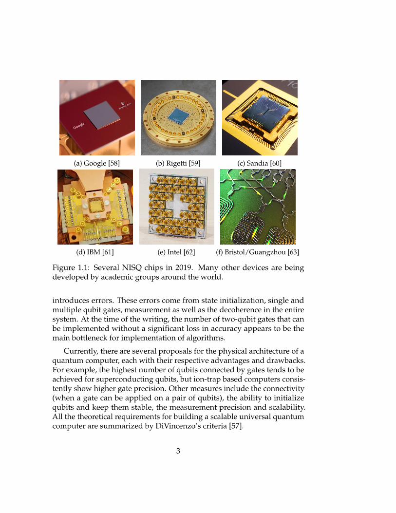
(a) Google [58] (b) Rigetti [59] (c) Sandia [60]
(d) IBM [61] (e) Intel [62] (f) Bristol/Guangzhou [63]
Figure 1.1: Several NISQ chips in 2019. Many other devices are beingdeveloped by academic groups around the world.
introduces errors. These errors come from state initialization, single andmultiple qubit gates, measurement as well as the decoherence in the entiresystem. At the time of the writing, the number of two-qubit gates that canbe implemented without a significant loss in accuracy appears to be themain bottleneck for implementation of algorithms.
Currently, there are several proposals for the physical architecture of aquantum computer, each with their respective advantages and drawbacks.For example, the highest number of qubits connected by gates tends to beachieved for superconducting qubits, but ion-trap based computers consis-tently show higher gate precision. Other measures include the connectivity(when a gate can be applied on a pair of qubits), the ability to initializequbits and keep them stable, the measurement precision and scalability.All the theoretical requirements for building a scalable universal quantumcomputer are summarized by DiVincenzo’s criteria [57].
3

On the superconducting front, companies such as Google [58], IBM [64],Intel [62] and Rigetti [65] are developing (or already developed) NISQ chips.We also see the renaissance of ion trap based computers with commercialefforts of ION-Q [66] and Honeywell [67]. Other architectures include pho-tonics, nuclear spins and NMR, analog quantum simulators and annealerssuch as the D-Wave machines.
It is not clear which hardware architecture is the most suitable for build-ing a quantum computer. It is also possible that future quantum computerswill consist of multiple types of quantum systems linked together. At thispoint, a quantum algorithm theorist such as myself can only speculate. Forthis reason, we focus on the development of hardware agnostic algorithms.
1.2 Quantum Computing Software in 2019
The capability of NISQ devices is in stark contrast with the requirements ofmost quantum algorithms. The quantum computing community works onclosing this gap from both sides – increasing the power of quantum devicesand decreasing the requirements of quantum algorithms.
The decline in the resource requirements of quantum algorithms hasbeen due to the developments in error correction, circuit synthesis, andquantum algorithms. As a consequence, the expected number of (physical)qubits required to break 2048-bit RSA was reduced from 1000 million in2012 [68] to 20 million while decreasing the overall computational time tounder 8 hours [69].
In this thesis, we focus on algorithmic improvements. One of the practi-cal applications we consider is the electronic structure problem in quantumchemistry. The goal is to efficiently estimate the ground state energy of agiven fermionic Hamiltonian given a description of the Hamiltonian and agood initial guess of the ground state (from an experiment or a mean-fieldcomputation). The problem stated this way has long been known to bepolynomially solvable on a quantum computer but it took over a decade ofresearch to decrease the powers of the polynomial [37, 70–74].
Code breaking (for example, factorization for breaking the RSA cryp-tosystem [75]) and quantum chemistry are two of the areas that can berevolutionized by quantum computing. We also expect improvements in
4
machine learning and optimization. All of the techniques in this thesiscan be used in one or more of these areas. We now proceed to give theiroverview.
1.3 Overview
During my PhD I co-authored the following publications.
• Sadegh Raeisi, Maria Kieferova, and Michele Mosca. Novel Tech-nique for Robust Optimal Algorithmic Cooling. Physical Review Letters,2019 [76].
• Maria Kieferova, Artur Scherer, and Dominic W Berry. Simulating thedynamics of time-dependent Hamiltonians with a truncated Dyson series.Physical Review A, 2019 [3]
• Yudong Cao, Jonathan Romero, Jonathan P Olson, Matthias Degroote,Peter D Johnson, Maria Kieferova, Ian D Kivlichan, Tim Menke, BorjaPeropadre, Nicolas PD Sawaya, Sukin Sim, Libor Veis, and AlanAspuru-Guzik. Quantum chemistry in the age of quantum computing.Chemical Reviews, 2018. [1].
• Dominic W Berry, Maria Kieferova, Artur Scherer, Yuval R Sanders,Guang Hao Low, Nathan Wiebe, Craig Gidney, and Ryan Babbush.Improved techniques for preparing eigenstates of fermionic Hamiltonian.npj Quantum Information, 2018 [2].
• Maria Kieferova and Nathan Wiebe. Tomography and generative trainingwith quantum Boltzmann machines. Physical Review A, 2017 [4].
• Maria Kieferova and Nathan Wiebe. On the power of coherently con-trolled quantum adiabatic evolutions. New Journal of Physics, 2014 [77]
Publications [2–4] constitute the research results presented this thesis.Publication [1] is a review of contemporary quantum computing techniquesfor quantum chemistry. Publication [77] came from my Master’s thesis andI finished it during the first months of my PhD. Publication [76] was an early
5

project unrelated to my other research and has been recently published inPhysical Review Letters.
This thesis is organized as follows. First, we review the existing algo-rithmic techniques in Chapter 2. Specifically, we review preliminaries inSection 2.1, give a brief overview of commonly used components of quan-tum algorithms in Section 2.2 and summarize the progress in Hamiltoniansimulation in Section 2.3.
The original research from my PhD is the content of Chapters 3 – 5.
Chapter 3 gives coherent versions of sorting and shuffling algorithms,including detailed circuits for their implementation. We also show that aninverse sort can be used as a shuffle. We then use the coherent shuffle forpreparation of a completely antisymmetric state in quantum chemistry.
Chapter 4 focuses on the simulation of time-dependent Hamiltonians.Such Hamiltonians arise whenever time-dependent fields or moving nucleiare involved, in simulations in the interaction picture and for digitallysimulating adiabatic evolution.
In Chapter 5 we introduce a quantum algorithm that can learn directlyfrom quantum data. We generalize the concept of a training set into a quan-tum context and show how to represent classical data in this framework.At the same time, our machine learning algorithm gives a new approach totomography. For readers unfamiliar with machine learning techniques weincluded a brief introduction in Appendix A.
I conclude this thesis by reviewing the results and presenting a list ofopen questions.
1.4 Notation
We now briefly review the notation used in this thesis:
• All logarithms are base 2 unless specified otherwise.
• We use the big-O notation to specify asymptotic upper bounds andΩstands for asymptotic lower bounds.
6
• As is customary in quantum computing, the symbol H can stand bothfor the Hadamard gate, in the context of quantum circuits, and aHamiltonian, if talking about the evolution of quantum systems. Thecorrect meaning of H should be clear from the context.
• We occasionally refer to complexity classes such asNP or BQP. Thedefinition of these classes can be found in standard textbooks or theComplexity Zoo [78].
7

2Background
“I love my computer and its software;I hug it often though it won’t care.I love each program and every file,I’d love them more if they worked a while.”
Dr. Seuss, The Lost Dr. Seuss Poem
In this chapter, I review the preliminaries and landmark results used inthe rest of the thesis. I start by introducing the circuit model, the notion ofcomplexity and fault-tolerance. Next, I review techniques used in my workincluding quantum simulation of classical computation, phase estimation,and amplitude amplification. The last section focuses on the developmentof Hamiltonian simulation that is heavily featured in my work. This re-view serves as a background for algorithms in Chapters 3-5 and is notintended for a quantum computing novice. For a pedagogical introductionto quantum computing and quantum algorithm please see [79–81] or referto quantum algorithm reviews [82–85].
8

2.1 Preliminaries
2.1.1 Quantum Gates and the Circuit Model
The first concept we need to introduce is a quantum bit, qubit. A classicalbit can be either in state 0 or 1. A qubit can be in any superposition of thesestates.
Qubit states are typically expressed either as vectors or in Dirac notation.
The “classical” states are assigned notation |0〉 :=
(10
)for state 0 and
|1〉 :=(
01
)for state 1 in Dirac and vector notation respectively. These states
form the computational basis on a 2-dimensional Hilbert space.
A general qubit state can be expressed as a linear combination α |0〉+β |1〉 where α,β are complex numbers and |α|2 + |β|2 = 1. In the vectorform, a qubit can be expressed as a normalized C2 vector
|ψ〉 =(α
β
). (2.1)
With two bits, the potential computational states are 00, 01, 10 and 11.The state on two qubits can be expressed as α |00〉+β |01〉+ γ |10〉+ δ |11〉for arbitrary α,β,γ and δ that satisfy the normalization condition |α|2 +
|β|2 + |γ|2 + |δ|2 = 1. A state on n qubits is a superposition over 2n basisstates.
Operations on qubits can be expressed using quantum circuits, de-scribed through diagrams as in Fig. 2.1. Quantum circuits show how apotentially complicated operation can be broken down into elementarycomponents, analogously to logic circuits. The components of quantumcircuits are simple unitary operations called gates and measurements.
One has a lot of freedom to pick a set of gates used in an algorithm.The choice of gates is often informed by the physical architecture (i.e.,superconducting qubits vs. trapped ions) and error-correcting code. Arequirement is that the chosen set of gates is universal.
9

•
••
Figure 2.1: A quantum circuit consists of wires (qubits, represented ashorizontal lines) and gates (unitary operations, represented as boxes). Thecircuit represents a sequence of operations with time going from left to right.Some of the gates can be controlled which means that they are executedonly if the control bit is in a given state. We use a black full circle to indicatethat an operation is applied only if the control qubit is |1〉 and we use anempty circle for |0〉. The operation can act in superposition, i.e. if the controlqubit is in state α |0〉+β |1〉, the (full circle) controlled unitary U will act onthe target state |ψ〉 as (α |0〉+β |1〉) |ψ〉 → α |0〉 |ψ〉+β |1〉U |ψ〉. The spacecost of this circuit is 8, the time cost is 17, and the depth is 7, see definitionsbelow.
A universal set of gates [86, 87] is a finite set of gates such that anyfinite-dimensional unitary operation can be implemented as a circuit con-sisting only of gates from this set. One such set is depicted in Fig. 2.2.According to the Solovay-Kitaev theorem [88], any two universal sets ofgates can simulate each other with at most polylogarithmic overhead. Forconvenience, we often add Pauli matrices, phase gate (denoted S and equalto T2, see Fig. 2.2) and multiply-controlled-NOTs into our available gateset. Synthesizing quantum operations into elementary gates is an activearea of research [86, 89] with immense implications for near-term quantumdevices.
Quantum computation often requires the use of additional qubits knownas ancillae. They play the same role as a working memory in classical com-puting; many calculations can be more efficient if there is more spaceavailable. At the same time, a large number of ancillae is prohibitive forpractical purposes.
10

H =1√2
(1 11 −1
)
(a) Hadamard gate
T =
(1 00 eiπ/4
)
(b) T-gate.
• =
1 0 0 00 1 0 00 0 0 10 0 1 0
(c) Controlled Pauli X,also known as controllednot or CNOT
Figure 2.2: A universal set of gates consisting of Hadamard, T gate anda C-NOT. This set of gates is arguably the most common in theoreticalquantum computing.
Quantum states are converted into classical information through a mea-surement. In principle, it is always possible to delegate measurements tothe end of the circuit. However, it is often advantageous in practice tomeasure as soon as possible [90, 91].
2.1.2 Complexity
We calculate the cost of computation in terms of the required resources asa function of the length of the input and other relevant parameters (forexample, the required precision of computation ε). As such, complexityshows how the “difficulty” of the computation scales when the inputgrows. The space complexity refers to the number of qubits, while the timecomplexity (often referred to only as the complexity) gives the numberof gates. Often, multiple gates can be executed in parallel. The depth ofthe circuit then refers to the number of rounds or layers when gates wereapplied (see Fig. 2.1).
The number of required gates can differ based on the gate set one workswith. However, a consequence of the Solovay-Kitaev theorem is that thisdifference is at most O (logc (1/ε)) for c > 1. In practice, not all gates arecreated equal. On near-term noisy devices (with no error correction) [54],two-qubit gates are the most common bottleneck. One may thus wish tominimize the number of two-qubit gates instead of gates in general. Forfault-tolerant computation based on the surface code [92], gates such as
11
T or Toffoli are several hundred times more expensive than Hadamard,Paulis, CNOT and other gates from Clifford group [93, 94].
Apart from gates, it is possible to include oracles (sometimes also calledblack boxes) in computation. An oracle is an abstract operation that canperform a given computation in a unit of time. We refer to the number ofqueries to the oracle as the query complexity. There are several reasonswhy one wants to include oracles in an algorithm. An oracle can repre-sent a separate computational primitive whose implementation can vary.For example of such oracles are common in Hamiltonian simulation; seeSubsection 2.3.1. An oracle can be given as a part of the definition of theproblem. In this case, one can have oracular access to a function, and ourgoal is to determine some properties of this function as in Deutsch-Joza [8]or Simon’s [11] algorithms. Finally, oracles are often used in the theoryof computational complexity to quantify the difficulty of tasks. One canconstruct a hierarchy of computational difficulty with respect to more andmore powerful oracles [95].
2.1.3 Error Correction and the Threshold Theorem
In the real world, neither the qubits nor the operations on them will beimplemented perfectly. There are a plethora of complications that comeinto engineering quantum devices, starting from the difficulty of fabricationthrough creating a well-isolated environment to the limited life of the qubits.Besides, all operations are imprecise, and the qubit-qubit interactions arethe obvious bottleneck for most implementations. These errors accumulatethroughout a computation, making a straightforward implementation ofan algorithm fail even for modestly sized circuits.
Fortunately for us, if the errors are below a given threshold, it is possibleto correct for them faster than they occur. The above statement is maderigorous in the quantum threshold theorem [96].
Theorem 1 (Quantum threshold theorem [96] , Theorem 10 in [97])There is a threshold error rate pT . Suppose we have a local stochastic error modelwith pi 6 p < pT
1. Then for any ideal circuit C, and any ε > 0, there exists
1Here pi is the probability of an uncorrelated error at a location Ci, see Definition 11in [97].
12

a fault-tolerant circuit C ′, which, when it undergoes the error model, producesan output which has statistical distance at most ε from the output of C. C ′ hasa number of qubits and a number of timesteps which are at most polylog(|C| /ε)times bigger than the number of qubits and timesteps in C, where |C| is the numberof locations in C.
Figure 2.3: Illustration of the difficulty of applying fault-tolerant T gatesfrom [73, Fig. 24]. The figure depicts a “T-factory” in surface code prepar-ing |T〉 states where |T〉 = cosβ |0〉+ eiπ/4 sinβ |1〉 and cos (2β) = 1√
3. One
|T〉 can be used for fault-tolerant implementation of one T gate [93]. Im-plementation of T (or different non-Clifford) gates are the bottleneck forfault-tolerant algorithms.
Several things need to be pointed out in the threshold theorem. Thefirst thing is the exact meaning of error rate and how would one estimate it;see [96, 98] for more detail. The second thing is the noise model. Makingassumptions about the noise, particularly its locality, is necessary. Thereis some evidence that error correction for a specific type of non-localizednoise might not be possible [99, 100]. In contrast, one can correct errorsmore effectively given additional promises about the error model. The lastand most commonly examined one is how would one go about devisingthe circuit C ′. Quantum error correction and fault-tolerant gadgets addressthis point.
The main idea is to use redundancy to encode a logical qubit into a
13
collection of physical qubits. The logical qubit is then encoded into non-local properties of the collection of physical qubits, making it resilient tolocalized errors. The first example of an error correcting code was Shor’s9-qubit code [101].
Currently, most of practical error correction uses topological codes [102,103], most prominently surface codes [68, 104, 105] with the stabilizer for-malism [94]. Broadly speaking, stabilizers allow us to detect errors withoutdisrupting the computation. Importantly, detecting and correcting errorscan be done efficiently.
Surface codes allow us to fault-tolerantly implement logical qubits intophysical qubits on a 2-D lattice, which makes them a prime candidate forerror correction in superconducting qubits. Even then, the typical ratiobetween physical and logical qubits can be of the order of thousands2.
Clifford gates (i.e., Paulis, H, S and CNOT) can be fault-tolerantly im-plemented in surface codes quite easily. However, it is necessary to includenon-Cliffords gates such as the T gate or Toffoli which are implementedusing magic states and fault-tolerant gadgets [93]. To illustrate the diffi-culty of implementing a T gate, we included a picture demonstrating itsimplementation in a surface code (see Fig. 2.3). Consequently, the cost ofcomputation is predominantly determined by the number of T gates.
We could not possibly give justice to fault-tolerance by such a briefoverview. For a more in-depth introduction to error correction see [68, 94]or any of the cited references.
2.2 A Brief Overview of Quantum Algorithms
The speedup in many algorithms stems from a smart application of severalquantum transformations. In this chapter, we give an overview of the mostused computing primitives and their applications.
2A recent result [69] uses 1568 physical qubits for each logical qubit. This estimate useslattice surgery and code distance d = 27.
14

••
=
1 0 0 0 0 0 0 00 1 0 0 0 0 0 00 0 1 0 0 0 0 00 0 0 1 0 0 0 00 0 0 0 1 0 0 00 0 0 0 0 1 0 00 0 0 0 0 0 0 10 0 0 0 0 0 1 0
Figure 2.4: The Toffoli gate, also known as doubly-controlled-NOT is uni-versal for classical computation and reversible.
2.2.1 Coherent Classical Computation
Before we move onto quantum algorithm primitives, let us review howa quantum computer can simulate classical computation. Examples ofclassical computation in quantum algorithms include logic, arithmetic orintegral evaluation. In this thesis, we propose coherent versions of classicalsorting and shuffling algorithms in Chapter 3.
Even though these algorithms do not provide a speedup comparedto their classical counterparts, they are often an unavoidable part of acomputation. For example, quantum chemistry algorithms such as theone in [73] require integral evaluation to compute matrix elements of theHamiltonian. Calculating them classically in advance and accessing themfrom a lookup table would asymptotically increase the complexity of thealgorithm; hence, the integrals are coherently evaluated on the quantumcomputer.
One of the inspirations for quantum computing was the work by Tof-foli [106], Fredkin [107], Landauer [108], Bennett [109, 110] and others onclassical reversible computation and its connection to thermodynamics andinformation theory. The reversible Toffoli gate (Fig. 2.4) is universal forclassical computation because it can simulate the NAND logic gate; seeFig. 2.5. As such, reversible computation is equivalent to classical compu-tation. Since the Toffoli can be also be implemented as a quantum gate,reversible computation gives us a way to construct classical computingprimitives in quantum circuits.
15

The downside of replacing NAND gates with Toffolis is the number ofadditional bits. The NAND logic gate takes two bits as inputs and outputsone bit, whereas the Toffoli has three qubits on both the input and output.This means that the number of ancillae would increase linearly with thenumber of gates in this naive construction. Such a construction quicklybecomes wasteful for large circuits or if space is limited. One can saveancillae by reversing the computation to uncompute the information savedin these registers [86, 111] and disentangle them from the output. Thesetechniques are crucial in algorithm design, and we use them in Chapter 4.
a • a
b • b
1 1⊕ (a∧ b) = a∧ b
Figure 2.5: A single Toffoli can replicate the NAND operation. The inputsof NAND stay unchanged and the result is encoded into an ancilla.
The space limitation is crucial for the practicability of near-term quan-tum computers; even modest constant factors can make a difference forimplementation on near-term hardware.
Several lines of research aim to make a quantum simulation of classicalcomputation. The use of additional gates, such as NOT or CNOT resultsin simpler circuits than a naive construction with only Toffolis [112–114].NOT and CNOT map computational basis states onto computational states;this means that they can be regarded as classical gates. Next, there has beensignificant effort to efficiently replicate classical computation using quan-tum components (such as Hadamards or T gates [115] ). Lastly, it is oftenpreferred to avoid arithmetic and classical computation altogether [116].
2.2.2 Phase Estimation and Eigenstate Preparation
Another widely used component of algorithms is phase estimation [117,118]. Given a unitary U and its eigenstate |ψθ〉 satisfying
U |ψθ〉 = ei2πθ |ψθ〉 , (2.2)
16

phase estimation can prepare with high probability the state |ψθ〉 |θ〉, whereθ is an m-digit approximation of θ. It can be shown that if we allowfor a failure rate at most ε, the algorithm requires n = m+
⌈log(2 + 1
ε
)⌉
additional qubits (not including the qubits needed to encode |ψ〉), 2n queriesto controlled U, and O
(n2) elementary gates. We assume that we are given
an oracle to implement controlled U. The circuit implementing phaseestimation is pictured in Fig. 2.6.
|0〉 H • . . .
QFT−1|0〉 H • . . .
|0〉 H . . . •
|ψ〉 U⊗2n−1U⊗2n−2 . . . U
Figure 2.6: Eigenvalue estimation circuit. The last block represents theinverse quantum Fourier transform depicted in Fig. 2.2.2.
Phase estimation starts by creating a uniform superposition on theancillary register by applying a Hadamard gate on each ancilla qubit.
|00 . . . 0〉 |ψ〉 → 1√2n
2n−1∑k=0
|k〉 |ψ〉 . (2.3)
In the next step, controlled U2j operations are applied.
1√2n
2n−1∑k=0
|k〉 |ψ〉 → 1√2n
2n−1∑k=0
|k〉Uk |ψ〉 (2.4)
=1√2n
2n−1∑k=0
|k〉 ei2πkθ |ψ〉 . (2.5)
The last part of phase estimation is the application of the inverse Fouriertransform (QFT−1, defined below). If θ can be expressed exactly in n bits, θ
17
would be equal to θ. Otherwise, θ is an m-digit approximation distributedaround θ.
The inverse quantum Fourier transform in the group Z2n (all we needin this case) is defined as
QFT−12n : |x〉 → 1√
2n
2n−1∑y=0
e−2πi x2n y |y〉 , (2.6)
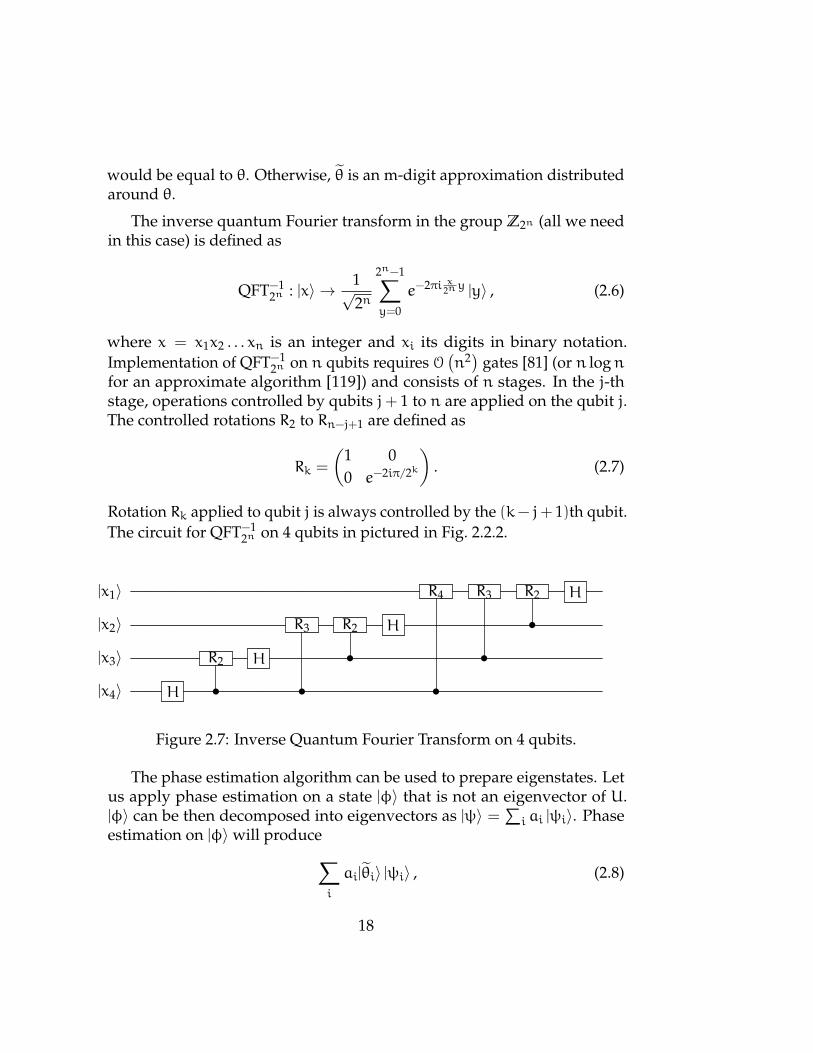
where x = x1x2 . . . xn is an integer and xi its digits in binary notation.Implementation of QFT−1
2n on n qubits requires O(n2) gates [81] (or n logn
for an approximate algorithm [119]) and consists of n stages. In the j-thstage, operations controlled by qubits j+ 1 to n are applied on the qubit j.The controlled rotations R2 to Rn−j+1 are defined as
Rk =
(1 00 e−2iπ/2k
). (2.7)
Rotation Rk applied to qubit j is always controlled by the (k− j+ 1)th qubit.The circuit for QFT−1
2n on 4 qubits in pictured in Fig. 2.2.2.
|x1〉 R4 R3 R2 H
|x2〉 R3 R2 H •
|x3〉 R2 H • •
|x4〉 H • • •
Figure 2.7: Inverse Quantum Fourier Transform on 4 qubits.
The phase estimation algorithm can be used to prepare eigenstates. Letus apply phase estimation on a state |φ〉 that is not an eigenvector of U.|φ〉 can be then decomposed into eigenvectors as |ψ〉 =∑i ai |ψi〉. Phaseestimation on |φ〉will produce∑
i
ai|θi〉 |ψi〉 , (2.8)
18
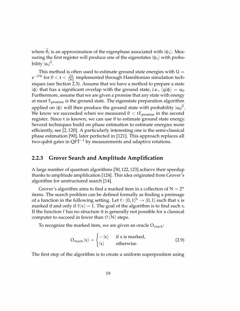
where θi is an approximation of the eigenphase associated with |ψi〉. Mea-suring the first register will produce one of the eigenstates |ψi〉 with proba-bility |ai|
2.
This method is often used to estimate ground state energies with U =e−iHt for 0 < t < 2π
‖H‖ implemented through Hamiltonian simulation tech-niques (see Section 2.3). Assume that we have a method to prepare a state|φ〉 that has a significant overlap with the ground state, i.e., 〈g|φ〉 = a0.Furthermore, assume that we are given a promise that any state with energyat most Epromise is the ground state. The eigenstate preparation algorithmapplied on |φ〉 will then produce the ground state with probability |a0|
2.We know we succeeded when we measured θ < tEpromise in the secondregister. Since t is known, we can use θ to estimate ground state energy.Several techniques build on phase estimation to estimate energies moreefficiently, see [2, 120]. A particularly interesting one is the semi-classicalphase estimation [90], later perfected in [121]. This approach replaces alltwo-qubit gates in QFT−1 by measurements and adaptive rotations.
2.2.3 Grover Search and Amplitude Amplification
A large number of quantum algorithms [50, 122, 123] achieve their speedupthanks to amplitude amplification [124]. This idea originated from Grover’salgorithm for unstructured search [14].
Grover’s algorithm aims to find a marked item in a collection ofN = 2n
items. The search problem can be defined formally as finding a preimageof a function in the following setting. Let f : 0, 1n → 0, 1 such that x ismarked if and only if f(x) = 1. The goal of the algorithm is to find such x.If the function f has no structure it is generally not possible for a classicalcomputer to succeed in fewer than O (N) steps.
To recognize the marked item, we are given an oracle Omark:
Omark |x〉 =− |x〉 if x is marked,|x〉 otherwise.
(2.9)
The first step of the algorithm is to create a uniform superposition using
19
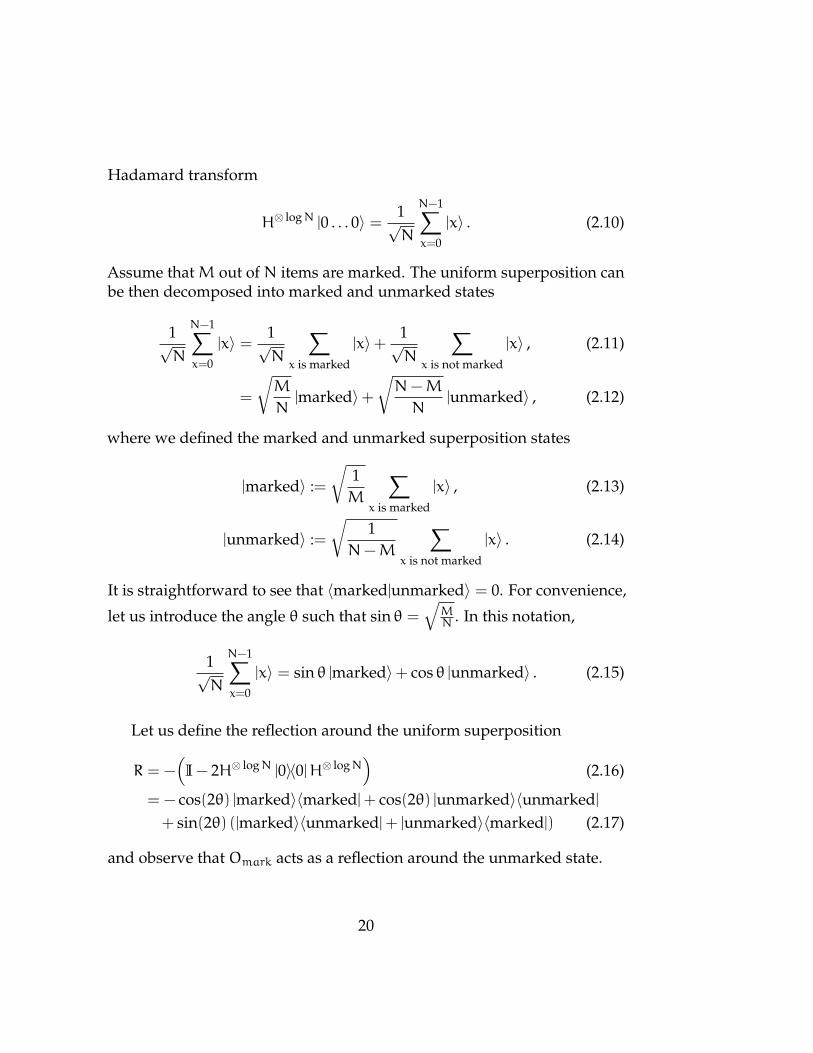
Hadamard transform
H⊗ logN |0 . . . 0〉 = 1√N
N−1∑x=0
|x〉 . (2.10)
Assume thatM out of N items are marked. The uniform superposition canbe then decomposed into marked and unmarked states
1√N
N−1∑x=0
|x〉 = 1√N
∑x is marked
|x〉+ 1√N
∑x is not marked
|x〉 , (2.11)
=
√M
N|marked〉+
√N−M
N|unmarked〉 , (2.12)
where we defined the marked and unmarked superposition states
|marked〉 :=√
1M
∑x is marked
|x〉 , (2.13)
|unmarked〉 :=√
1N−M
∑x is not marked
|x〉 . (2.14)
It is straightforward to see that 〈marked|unmarked〉 = 0. For convenience,
let us introduce the angle θ such that sin θ =√MN . In this notation,
1√N
N−1∑x=0
|x〉 = sin θ |marked〉+ cos θ |unmarked〉 . (2.15)
Let us define the reflection around the uniform superposition
R = −(
I − 2H⊗ logN |0〉〈0|H⊗ logN)
(2.16)
= − cos(2θ) |marked〉〈marked|+ cos(2θ) |unmarked〉〈unmarked|+ sin(2θ) (|marked〉〈unmarked|+ |unmarked〉〈marked|) (2.17)
and observe that Omark acts as a reflection around the unmarked state.
20

We can show show that the operation G = ROmark acts as a rotation byan angle 2θ on the subspace span|marked〉 , |unmarked〉. Let us apply Gon an arbitrary state |ψ〉 = sinα |marked〉+ cosα |unmarked〉:
G |ψ〉 = ROmark(
sinα |marked〉+ cosα |unmarked〉)
(2.18)
= R(− sinα |marked〉+ cosα |unmarked〉
)(2.19)
= sinα(cos(2θ) |marked〉− sin(2θ) |unmarked〉)− cosα(− cos(2θ) |unmarked〉− sin(2θ) |marked〉) (2.20)
= sin (α+ 2θ) |marked〉+ cos (α+ 2θ) |marked〉 (2.21)
It can be shown that span|marked〉 , |unmarked〉 is closed under theapplication of G. Thus, G rotates the initial state towards |marked〉. Assum-
ing that√
NM 1, this requires approximately π
4
√MN applications of G. In
the case where M N, Grover’s algorithm achieves quadratic speedupover any classical algorithm.
Grover search can be generalized to amplitude amplification. Ampli-tude amplification can be used to boost the success amplitude for a widevariety of quantum computations. Let us take a unitary U that prepares astate that has λ overlap with the desired state |good〉 and can be thereforewritten as
U |0 . . . 0〉 = sin θ |good〉+ cos θ |bad〉 , (2.22)
where 〈good|bad〉 = 0. In this notation, θ = π2 means that we reached the
desired state |good〉 with certainty. Given reflections around the zero stateR0 = I − 2 |0〉〈0| and the correct state Rgood = I − 2 |good〉〈good| we canthen construct the operatorG = UR0U
−1Rgood. The operatorG is analogousto Grover’s operator – the same type of calculation can be used to provethe correctness of the algorithm. Reaching a high probability of successrequires approximately π
4θ applications of G.
The presented versions assume that the fraction of marked items MN
and the initial overlap is known. The initial amplitude can be estimatedusing quantum amplitude estimation [79]. Alternatively, a more technicalversion of amplitude amplification can be used instead [125] to avoidover-rotating. Another extension of amplitude amplification is obliviousamplitude amplification which we discuss in the next section.
21
2.2.4 Oblivious Amplitude Amplification
Oblivious amplitude amplification (OAA) extends the framework of am-plitude amplification by relaxing the requirement on the reflection. Whileamplitude amplification reflects around the good state, |good〉, OAA re-flects only around a control system, leaving the target system untouched.OAA then allows us to turn a probabilistic implementation of an opera-tion [77, 126] into a nearly perfect one without an exponential overhead.
Suppose thatW probabilistically implements U such as
W |0〉flag |ψ〉data = sin θ |0〉flagU |ψ〉data + cos θ |bad〉 , (2.23)
where(|0〉〈0|flag ⊗ Idata
)|bad〉 = 0. In other words, if we measure the
ancilla in state |0〉, Uwas properly applied on |ψ〉data.
Berry et al. showed in [34] thatWRW†R acts as a rotation(WRW†R
)kW |0〉 |ψ〉 = sin ((2k+ 1)θ) |0〉U |ψ〉+ cos ((2k+ 1)θ) |bad〉 ,
(2.24)where R is the reflection around all zero in the flag register R = 2 |0〉〈0|⊗ I−I. Note that oblivious amplitude amplification differs from amplitude am-plification in that R is not a reflection around the initial state. Nevertheless,using a different reflection is in this case sufficient.
In addition, one can show that it is sufficient to constrain ourselvesto span|0〉U |ψ〉 , |bad〉. Success amplitude sin((2k+ 1)θ) can be then beboosted arbitrarily close to 1.
So far we assumed that U is a unitary operation. It turns out thatoblivious amplitude amplification is robust, meaning that it can handleoperations that is only ε close to a unitary [34]. At the same time, W isstill a unitary operator. Amplification will in this case not be performedperfectly, but the error is at most O(ε).
2.3 Hamiltonian Evolution Simulation
This section focuses on the problem of simulating the dynamics of a quan-tum system. Given an initial state of a system |ψ(0)〉 and a Hamiltonian H,
22

our aim is to simulate the time evolution |ψ(0)〉 → e−iHt |ψ(0)〉. The goalof Hamiltonian simulation is to design a circuit U consisting of gates andoracles that approximates the time evolution up to an error ε such that
∥∥∥U− e−iHt∥∥∥
2< ε, (2.25)
where ‖·‖2 is the spectral norm3. We predominantly focus on the querycomplexity of Hamiltonian simulation.
In Chapter 4 we present a simulation algorithm for a time-dependentHamiltonian which is an extension of the above-stated problem. Here wepresent techniques used or related to those in Chapter 4.
Quantum systems are fundamentally difficult to simulate; dynamicsof quantum systems is a BQP-hard (or BQP complete for Hamiltonianswith natural restrictions) [6, 28, 128]. Even though there are certain cases,such as Clifford circuits [129], when a classical simulation is possible, thecomplexity of simulating the evolution generally grows exponentially withthe number of qubits.
As such, simulation of quantum dynamics is a field where we believequantum computers can quickly outperform classical ones. In fact, the timeevolution of quantum systems was the original application for quantumcomputers suggested by Feynman in his seminal paper [130] and Lloyd’salgorithm [13] from 1996 was one of the early quantum algorithms withexponential speedup.
We start this section by defining the formalism and establishing simula-tion lower bounds. Then, we follow the chronological progress of Hamil-tonian simulation research, starting by Lloyd’s [13] paper and follow-upapproaches based on Lie-Trotter formula, often referred to as Trotterizationor product formulae.
Early Hamiltonian simulation algorithms assumed that the simulatedHamiltonians are given in the formH =
∑mj=1Hj, where eachHj is local and
3Spectral norm is the correct measure even for algorithms that involve measurementson ancillae. In this case, the diamond norm
∥∥U− e−iHt∥∥3
would be an appropriatemeasure but it can be bounded by 4
∥∥U− e−iHt∥∥
2 [127]. The proof involves writing thesimulation algorithm as a channel where the desired operation (to be applied after post-selection on a measurement outcome) is one of the Kraus operators. The diamond norm isthen bounded using norm inequalities and strong convexity.
23

e−iHjt can be implemented directly for arbitrary t. The complexity of thesealgorithms was then generally measured by the number of exponentialsneeded for the simulation [29]. Nowadays, we do not take these assump-tions for granted and instead only assume that the Hamiltonian is a sparseHermitian matrix and its elements can be accessed through oracles, seeSec. 2.3.1. Non-local Hamiltonians appear in quantum chemistry [131, 132]and applications outside of physics such as digital simulation of adiabaticcomputation [133] and systems of linear equations [5, 134]. The complexityof a simulation algorithm is then measured predominantly in terms oforacle queries and then in terms of additional gates [31, 33, 127]. This willbe the convention we follow in this thesis. Of course, there are exceptionsto this rule, particularly if the authors are interested in a more specializedclass of Hamiltonians.
Simultaneously with the development of Trotterization algorithms,Childs suggested a simulation algorithm based on quantum walks [126]. In2014, a seminal paper by Berry et al. [135] achieved exponential improve-ment in the error scaling and was subsequently improved upon in [34, 136].In the last few years, approaches based on singular value processing [35]and qubitization [137] achieved the optimal query complexity.
Let us note that Hamiltonian simulation is often used as a subroutine ofa more complex algorithm, for example in phase estimation (described inSection 2.2.2) or for solving linear equations [5, 134].
This section is based on part 4.1 of Quantum Chemistry in the Age ofQuantum Computing [1] but it has been significantly extended and altered.It aims to provide an overview of the existing results from the conceptionof Hamiltonian simulation to the most recent results. To the best of ourknowledge, there are no current surveys covering recent techniques suchas quantum signal processing and linear combinations of unitaries (LCU)methods. The older reviews of Hamiltonian simulations include Berry etal. [138] and Georgescu et al. [139].
2.3.1 The Hamiltonian Oracles
In this section, we explain how one can grant access to a Hamiltonian.The oracular representation allows us to work with Hamiltonians thatare not necessarily local, for example in adiabatic computation [133] or
24
quantum chemistry [140]. Storing the Hamiltonian as a full matrix wouldnot be practical because storing such a representation would necessarilyrequire an exponential overhead. Instead, oracles often provide access tothe Hamiltonian as an abstraction for computing the matrix elements asdiscussed in Section 2.1.2.
One type of oracular access is particularly common when the Hamil-tonian (in a computational basis) is given by a sparse matrix. We say aHamiltonian is row-d-sparse if each row has at most d non-zero entries. Ifthere is an efficient procedure to locate these entries we moreover say thatthe Hamiltonian is row-computable. In this case, one can efficiently constructoracles
Oloc |r,k〉 = |r,k⊕ l〉 (2.26)Oval |r, l, z〉 = |r, l, z⊕Hr,l〉 . (2.27)
OracleOloc locates the position l of the k-th non-zero element in row r. Theoracle Oval then gives the value of the matrix element Hr,l. We computethe cost of algorithms in terms of the number of queries to these oracles.
It is possible to construct different oracles. Any Hermitian matrix canbe decomposed into a sum of unitaries
H =
L−1∑l=0
αlHl, (2.28)
where for each l, αl 6 0 and Hl is a unitary matrix ‖Hl‖ = 1. This decom-position can be efficiently implemented for sparse Hamiltonians [34]. Thecoefficients αl and unitaries Hl can be accessed through oracles
Oα |l, z〉 = |l, z⊕αl〉 (2.29)OHl |l,ψ〉 = Hl |l,ψ〉 , (2.30)
or, in some cases, described classically.
Berry et al. introduced the decomposition (2.28) in [135] and showedthat for d-sparse Hamiltonians, L can be chosen as L = O
(d2 ‖H‖max /γ
),
where γ is the precision with which the Hamiltonian matrix entries areapproximated. Furthermore, oracles (2.29) and (2.30) can be simulated byoracle queries to (2.26) and (2.27) with constant overhead.
25
Lastly, Low and Chuang [137] introduced a representation of a Hamilto-nian through a signal oracle U such that for a signal state defined as |G〉,H = 〈G|U |G〉. In other words,
U |G〉 |ψ〉 = |G〉H |ψ〉+√
1 − |H |ψ〉|2 |G⊥〉 , (2.31)
where(|G〉〈G|⊗ I
)|G⊥〉 = 0. This approach is based on the Hamiltonian
representation in the linear combination of unitaries (LCU) approach [135].This model is used heavily in algorithms based on quantum signal pro-cessing [36]. Low and Chuang [137] showed that the oracle (2.31) can beimplemented with O(1) queries to (2.29) and (2.30). This results allows us touse QSP with LCU [137] instead of the relying on an earlier implementationusing quantum walks [35].
Other models in quantum simulation include the fractional query model[135], representation of the Hamiltonian via a density matrix [141], or datastructures for non-sparse Hamiltonians [135], but do not appear in thealgorithms mentioned in this thesis.
2.3.2 Lower Bounds on Hamiltonian Simulation
Before describing any quantum algorithms, let us first establish what is thebest complexity we could hope for. All but one of the lower bounds in thissection are stated in the query complexity model. The first lower bound onHamiltonian simulation is known as the no-fast forwarding theorem [29]. Itestablishes that no quantum computer can simulate Hamiltonian evolutionfor time t with complexity sublinear in ‖H‖ t.
Berry, Ahokas, Cleve and Sanders (BACS) [29] proved the no-fast-forwarding theorem by reduction to the parity problem [142, 143]. Thework on the parity problem established that the parity of B bits cannotbe determined with fewer than B/2 queries (a query outputs a single bit)with 1/4 error. The authors [29] explicitly construct a 2-sparse Hamiltonianwhose sublinear simulation would imply a parity algorithm that uses fewerthan N/2 queries. However, there are still possible speedups for denseHamiltonians in other parameters besides time.
There were two important lower bounds following the landmark [29]result. Childs and Kothari [144] proved the restrictions for simulating dense
26
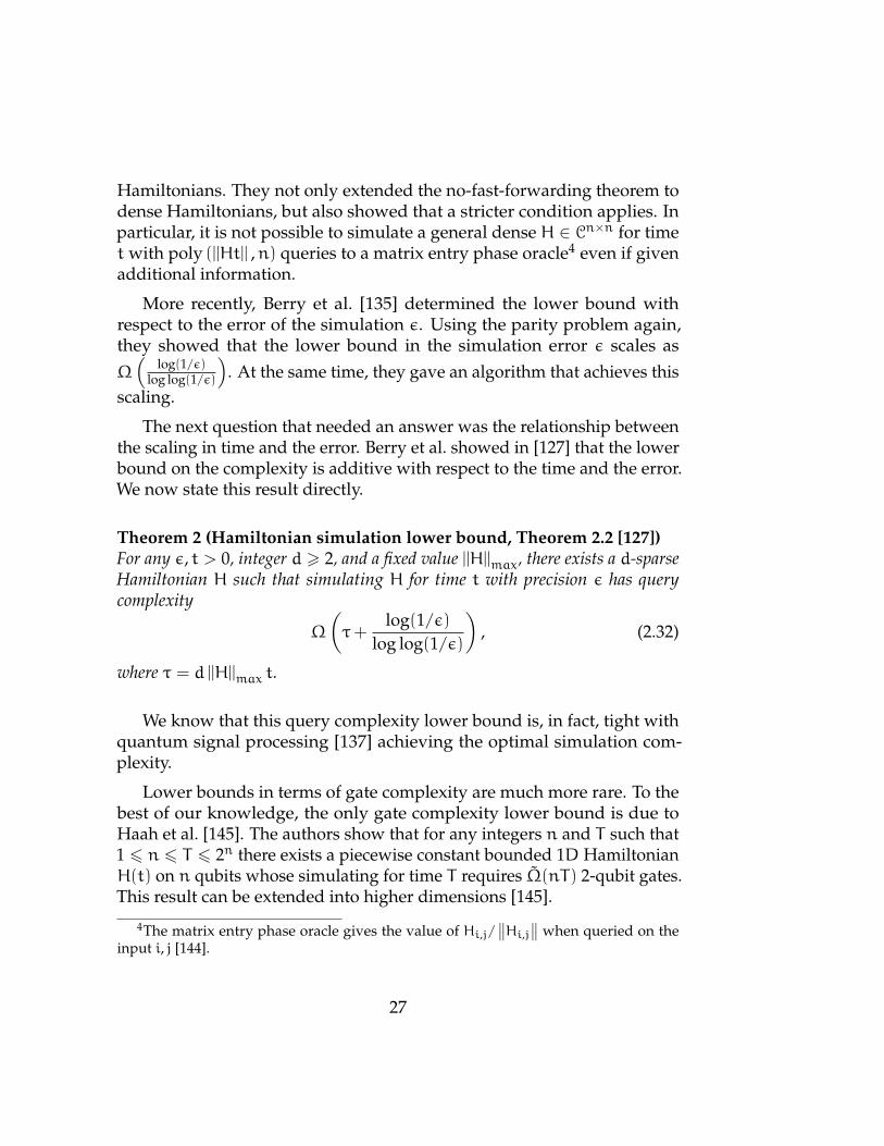
Hamiltonians. They not only extended the no-fast-forwarding theorem todense Hamiltonians, but also showed that a stricter condition applies. Inparticular, it is not possible to simulate a general dense H ∈ Cn×n for timetwith poly (||Ht|| ,n) queries to a matrix entry phase oracle4 even if givenadditional information.
More recently, Berry et al. [135] determined the lower bound withrespect to the error of the simulation ε. Using the parity problem again,they showed that the lower bound in the simulation error ε scales asΩ(
log(1/ε)log log(1/ε)
). At the same time, they gave an algorithm that achieves this
scaling.
The next question that needed an answer was the relationship betweenthe scaling in time and the error. Berry et al. showed in [127] that the lowerbound on the complexity is additive with respect to the time and the error.We now state this result directly.
Theorem 2 (Hamiltonian simulation lower bound, Theorem 2.2 [127])For any ε, t > 0, integer d > 2, and a fixed value ||H||max, there exists a d-sparseHamiltonian H such that simulating H for time t with precision ε has querycomplexity
Ω
(τ+
log(1/ε)log log(1/ε)
), (2.32)
where τ = d ||H||max t.
We know that this query complexity lower bound is, in fact, tight withquantum signal processing [137] achieving the optimal simulation com-plexity.
Lower bounds in terms of gate complexity are much more rare. To thebest of our knowledge, the only gate complexity lower bound is due toHaah et al. [145]. The authors show that for any integers n and T such that1 6 n 6 T 6 2n there exists a piecewise constant bounded 1D HamiltonianH(t) on n qubits whose simulating for time T requires Ω(nT) 2-qubit gates.This result can be extended into higher dimensions [145].
4The matrix entry phase oracle gives the value of Hi,j/∥∥Hi,j
∥∥ when queried on theinput i, j [144].
27

2.3.3 Simulation Based on Trotterization
The first quantum simulation algorithms relied on the lowest-order Lie-Trotter formula
eA+B = limr→∞
(eA/reB/r
)r. (2.33)
Lloyd [13] first showed how to use the Lie-Trotter formula for Hamilto-nian simulation. Assuming that the Hamiltonian of interest can be decom-posed into a sum of of simpler Hamiltonians5 Hj such that H =
∑mj=1Hj,
one can decompose the evolution with respect to H into the evolution withrespect to each Hj as
U =(e−iH1t/re−iH2t/r . . . e−iHmt/r
)r. (2.34)
If each e−iHjt/r can be efficiently implemented, one can simulate Hamil-tonian evolution using O (poly logN) steps as opposed to O (polyN) for aclassical simulation.
This approach can be extended to sparse matrices given through theoracles defined in (2.26) and (2.27). Aharonov and Ta-Shma [133] firstshowed that a sparse Hermitian matrix can be decomposed as H =
∑jHj,
where each eiHjt can be implemented directly. Then, using the Lie-Trotterformula, d-sparse Hamiltonians can be simulated with O(poly(N,d)(τ2/ε))complexity.
Two types of improvements were made since the first Trotterization-based simulations. A series of works by Berry, Wiebe, and others [29, 30]used more sophisticated Lie-Trotter-Suzuki decompositions [146]. Theseapproximations allow for the approximation error to be an inverse of apolynomial of arbitrary order by devising high-order formulae that betterapproximate an exponential of a sum. For illustration, the symmetricTrotter formula
e(A+B)∆t ≈ eA∆t/2eB∆teA∆t/2 (2.35)
suppresses O(∆t2) errors [30]. These higher-order formulae can be obtainedusing the recursion relation
S2k(δ) = [S2k−2(pkδ)]2 S2k−2((1 − 4pk)δ) [S2k−2(pkδ)]
2 , (2.36)5For example, if H is a sum of local terms as in the Ising model.
28
where
S2(δ) =
m∏j=1
eHjδ/21∏
j ′=m
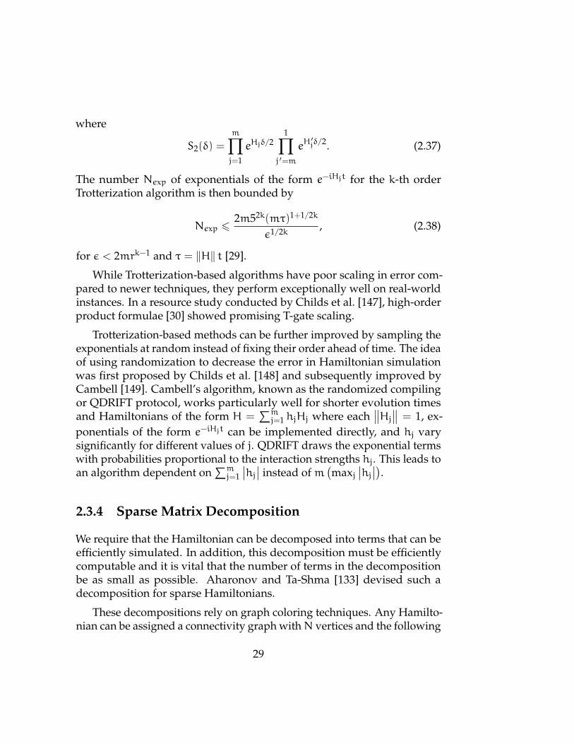
eH′jδ/2. (2.37)
The number Nexp of exponentials of the form e−iHjt for the k-th orderTrotterization algorithm is then bounded by
Nexp 62m52k(mτ)1+1/2k
ε1/2k , (2.38)
for ε < 2mrk−1 and τ = ‖H‖ t [29].
While Trotterization-based algorithms have poor scaling in error com-pared to newer techniques, they perform exceptionally well on real-worldinstances. In a resource study conducted by Childs et al. [147], high-orderproduct formulae [30] showed promising T-gate scaling.
Trotterization-based methods can be further improved by sampling theexponentials at random instead of fixing their order ahead of time. The ideaof using randomization to decrease the error in Hamiltonian simulationwas first proposed by Childs et al. [148] and subsequently improved byCambell [149]. Cambell’s algorithm, known as the randomized compilingor QDRIFT protocol, works particularly well for shorter evolution timesand Hamiltonians of the form H =
∑mj=1 hjHj where each
∥∥Hj∥∥ = 1, ex-
ponentials of the form e−iHjt can be implemented directly, and hj varysignificantly for different values of j. QDRIFT draws the exponential termswith probabilities proportional to the interaction strengths hj. This leads toan algorithm dependent on
∑mj=1∣∣hj∣∣ instead ofm
(maxj
∣∣hj∣∣).
2.3.4 Sparse Matrix Decomposition
We require that the Hamiltonian can be decomposed into terms that can beefficiently simulated. In addition, this decomposition must be efficientlycomputable and it is vital that the number of terms in the decompositionbe as small as possible. Aharonov and Ta-Shma [133] devised such adecomposition for sparse Hamiltonians.
These decompositions rely on graph coloring techniques. Any Hamilto-nian can be assigned a connectivity graph withN vertices and the following
29

12 3
4
567
8
9 10 11 12
1314
. 1 . . . . . . 11 . . . .1 . 1 . . . . . . . 1 . . 1. 1 . 1 . . . . . . 111 .. . 1 . 1 . . . . . . 1 . .. . . 1 . 1 . . . . . . 1 .. . . . 1 . 1 . . . . . 11. . . . . 1 . 111 . . . 1. . . . . . 1 . 11 . . . .1 . . . . . 11 . 1 . . . .1 . . . . . 111 . . . . 1. 11 . . . . . . . . 111. . 111 . . . . . 1 . 1 .. . 11 . 1 . . . . 11 . .. 1 . . . 11 . . 11 . . .
=
. 1 . . . . . . . . . . . .1 . . . . . . . . . . . . .. . . . . . . . . . . . 1 .. . . . . . . . . . . . . .. . . . . 1 . . . . . . . .. . . . 1 . . . . . . . . .. . . . . . . . . 1 . . . .. . . . . . . . . . . . . .. . . . . . . . . . . . . .. . . . . . 1 . . . . . . .. . . . . . . . . . . . . 1. . . . . . . . . . . . . .. . 1 . . . . . . . . . . .. . . . . . . . . . 1 . . .
+
. . . . . . . . 1 . . . . .
. . . . . . . . . . . . . .
. . . . . . . . . . . 1 . .
. . . . . . . . . . . . . .
. . . . . . . . . . . . . .
. . . . . . . . . . . . 1 .
. . . . . . . . . . . . . 1
. . . . . . . . . . . . . .1 . . . . . . . . . . . . .. . . . . . . . . . . . . .. . . . . . . . . . . . . .. . 1 . . . . . . . . . . .. . . . . 1 . . . . . . . .. . . . . . 1 . . . . . . .
+
. . . . . . . . . 1 . . . .
. . 1 . . . . . . . . . . .
. 1 . . . . . . . . . . . .
. . . . 1 . . . . . . . . .
. . . 1 . . . . . . . . . .
. . . . . . 1 . . . . . . .
. . . . . 1 . . . . . . . .
. . . . . . . . 1 . . . . .
. . . . . . . 1 . . . . . .1 . . . . . . . . . . . . .. . . . . . . . . . . 1 . .. . . . . . . . . . 1 . . .. . . . . . . . . . . . . .. . . . . . . . . . . . . .
+
. . . . . . . . . . . . . .
. . . . . . . . . . 1 . . .
. . . 1 . . . . . . . . . .
. . 1 . . . . . . . . . . .
. . . . . . . . . . . . . .
. . . . . . . . . . . . . 1
. . . . . . . . . . . . 1 .
. . . . . . . . . 1 . . . .
. . . . . . . . . . . . . .
. . . . . . . 1 . . . . . .
. 1 . . . . . . . . . . . .
. . . . . . . . . . . . . .
. . . . 1 . . . . . . . . .
. . . . . 1 . . . . . . . .
+
. . . . . . . . . . . . . .
. . . . . . . . . . . . . .
. . . . . . . . . . 1 . . .
. . . . . . . . . . . . . .
. . . . . . . . . . . . . .
. . . . . . . . . . . . . .
. . . . . . . . 1 . . . . .
. . . . . . . . . . . . . .
. . . . . . 1 . . . . . . .
. . . . . . . . . . . . . 1
. . 1 . . . . . . . . . . .
. . . . . . . . . . . . 1 .
. . . . . . . . . . . 1 . .
. . . . . . . . . 1 . . . .
+
. . . . . . . . . . . . . .
. . . . . . . . . . . . . 1
. . . . . . . . . . . . . .
. . . . . . . . . . . 1 . .
. . . . . . . . . . . . . .
. . . . . . . . . . . . . .
. . . . . . . 1 . . . . . .
. . . . . . 1 . . . . . . .
. . . . . . . . . 1 . . . .
. . . . . . . . 1 . . . . .
. . . . . . . . . . . . . .
. . . 1 . . . . . . . . . .
. . . . . . . . . . . . . .
. 1 . . . . . . . . . . . .
Figure 2.8: An example of Hamiltonian decomposition based on edgecoloring. The entire graph corresponds the full, black, matrix. The coloredmatrices then represent edges of a given color. Note that each coloredmatrix is only 1-sparse.
30
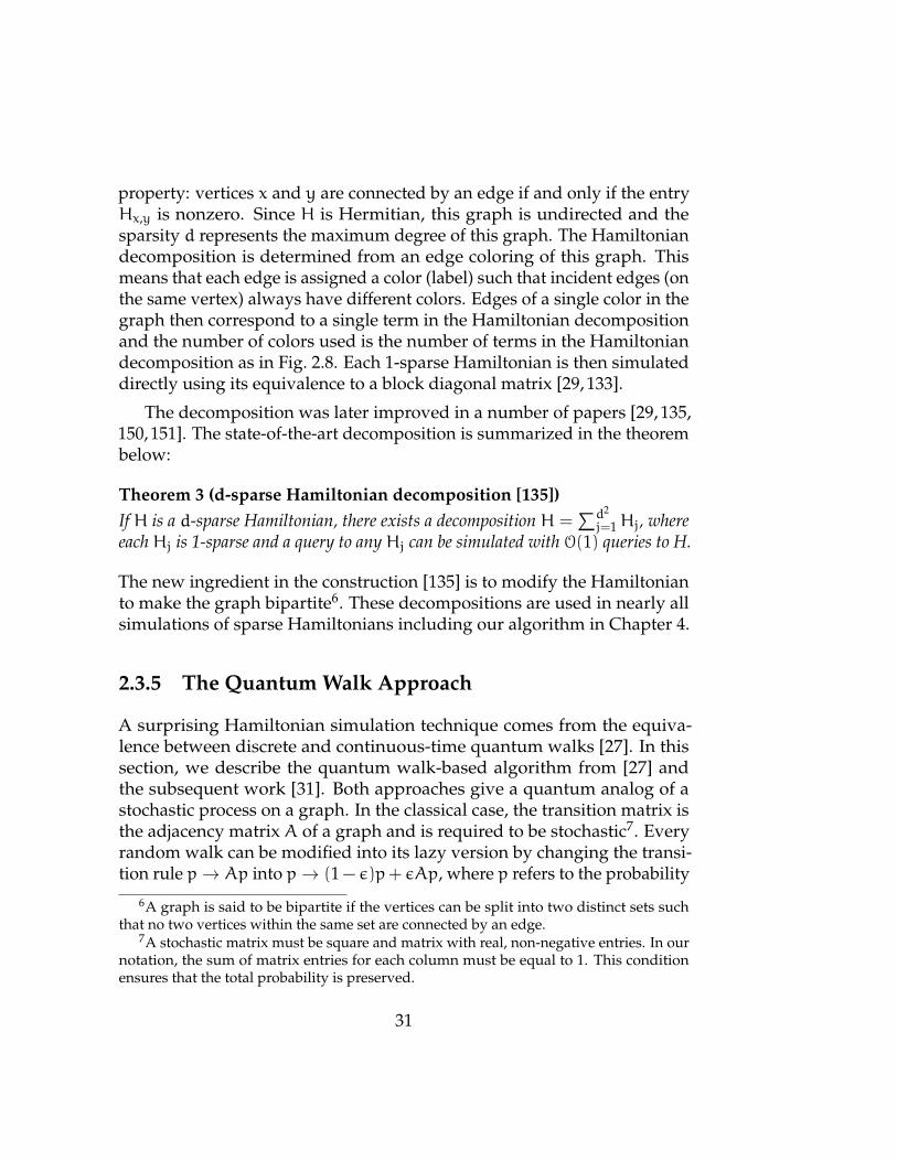
property: vertices x and y are connected by an edge if and only if the entryHx,y is nonzero. Since H is Hermitian, this graph is undirected and thesparsity d represents the maximum degree of this graph. The Hamiltoniandecomposition is determined from an edge coloring of this graph. Thismeans that each edge is assigned a color (label) such that incident edges (onthe same vertex) always have different colors. Edges of a single color in thegraph then correspond to a single term in the Hamiltonian decompositionand the number of colors used is the number of terms in the Hamiltoniandecomposition as in Fig. 2.8. Each 1-sparse Hamiltonian is then simulateddirectly using its equivalence to a block diagonal matrix [29, 133].
The decomposition was later improved in a number of papers [29, 135,150, 151]. The state-of-the-art decomposition is summarized in the theorembelow:
Theorem 3 (d-sparse Hamiltonian decomposition [135])If H is a d-sparse Hamiltonian, there exists a decomposition H =
∑d2
j=1Hj, whereeach Hj is 1-sparse and a query to any Hj can be simulated with O(1) queries to H.
The new ingredient in the construction [135] is to modify the Hamiltonianto make the graph bipartite6. These decompositions are used in nearly allsimulations of sparse Hamiltonians including our algorithm in Chapter 4.
2.3.5 The Quantum Walk Approach
A surprising Hamiltonian simulation technique comes from the equiva-lence between discrete and continuous-time quantum walks [27]. In thissection, we describe the quantum walk-based algorithm from [27] andthe subsequent work [31]. Both approaches give a quantum analog of astochastic process on a graph. In the classical case, the transition matrix isthe adjacency matrix A of a graph and is required to be stochastic7. Everyrandom walk can be modified into its lazy version by changing the transi-tion rule p→ Ap into p→ (1− ε)p+ εAp, where p refers to the probability
6A graph is said to be bipartite if the vertices can be split into two distinct sets suchthat no two vertices within the same set are connected by an edge.
7A stochastic matrix must be square and matrix with real, non-negative entries. In ournotation, the sum of matrix entries for each column must be equal to 1. This conditionensures that the total probability is preserved.
31

distribution on the graph and ε ∈ (0, 1). Taking the limit ε → 0 and aninfinitesimally short length of each step, one can obtain the continuoustime limit of a random walk
p(t) = eAtp0, (2.39)
which can be interpreted as the diffusion equation.
A continuous-time quantum walk [152] is obtained by replacing (2.39)by the Schrodinger equation
|ψ(t)〉 = e−iAt |ψ0〉 , (2.40)
with the adjacency matrix as the Hamiltonian. The Hamiltonian is Hermi-tian if the graph is undirected.
Discrete-time quantum walks take a very different approach. The con-struction by Szegedy [15] translates any Markov chain on a graph to aquantum process on a quadratically larger Hilbert space. Discrete-timequantum walks are typically defined on symmetric graphs but the construc-tion can be generalized to any N×NHamiltonian H. Using the notationfrom [27], define
∣∣ψj⟩=
1√‖abs(H)‖
N∑k=1
√H∗j,k
dkdj
|j,k〉 (2.41)
for every pair of graph vertices j,k where abs(H) stands for entry-wiseabsolute value of H and |d〉 =
∑j dj |j〉 is the principal eigenvector of
abs(H). This construction allows us to make the quantum walk unitary. Astate |k, j〉 can be assigned to an edge between k and j; j being the vertexwhere the walker starts in a particular step and k the vertex the walker ismoving towards. Let S be the swap operation of these registers
S |j,k〉 = |k, j〉 . (2.42)
Next, define an isometry T mapping the states of the graph onto thestates of enlarged Hilbert space
T =
N∑j=1
∣∣ψj⟩〈j| . (2.43)
32

One step of the walk can be implemented using iS(2TT † − I); see [15].Taking the eigenvalues of the Hamiltonian H
‖abs(H)‖ |λ〉 = λ |λ〉, it can beshown [153] that the eigenvectors of U = iS(2TT † − I) are
|µ±〉 =1 − e±i arccos λS√
2(1 − λ2)T |λ〉 (2.44)
and corresponding eigenvalues µ± = ±e±i arcsin λ [27].
Discrete-time quantum walks are already formulated in terms of querycomplexity. The framework of quantum walks [21], can be applied to avariety of classical randomized algorithms and gives a number of provablespeedups [15, 21, 154–156].
The relationship between discrete and continuous random walks trans-lates to a correspondence between discrete and continuous time quantumwalks. Childs quantified this correspondence devising an algorithm forsimulating continuous-time walks using discrete time quantum walks.Since discrete-time quantum walks can be easily translated into the gatemodel [157, 158], this result de facto gave a new algorithm for simulatingHamiltonian evolution [31].
Let us take |Θ〉 to be an eigenstate of a discrete time quantum walk withan eigenvalue e−iΘ. Furthermore, define P to be an operation that performsphase estimation on the walk and records the outcome in an additionalregister
P |Θ〉 =∑φ
aφ|Θ |Θ,φ〉 . (2.45)
Next, define a unitary Ftsin that computes the sine function and appliesan appropriate phase
Ftsin |Θ,φ〉 = e−it sinφ |Θ,φ〉 . (2.46)
Childs showed in [27] that Hamiltonian evolution can be closely ap-proximated using discrete-time quantum walk techniques
〈ψ|eiHtT †P†FtsinPT |ψ〉 > 1 −93t2
M2 , (2.47)
33

where M denotes the number of calls to quantum walk unitary U. Equa-tion (2.47) shows that the fidelity between states produced by the quantumwalk algorithm and time evolution is high. TakingM = O
(t√δ
), Hamilto-
nian evolution for time t can be simulated using O(∥∥∥abs(H)t/
√δ∥∥∥)
stepsof a discrete-time quantum walk.
Reference [27] just considered the complexity in terms of the steps of thisdiscrete quantum walk, without showing how to implement them. Berryand Childs [31] provided methods to implement the discrete quantum walkin terms of the oracles for matrix entries of the Hamiltonian (2.26), (2.27),thus providing a complexity that could be compared to the prior workbased on Trotterization. Quantum-walk simulation techniques have querycomplexity linear in simulation time compared to superlinear complexityfor Trotterization methods [29].
2.3.6 Hamiltonian Simulation with Linear Combination ofUnitaries
We now present a Hamiltonian simulation algorithm [34] that achievesa logarithmic scaling in the inverse error. This algorithm requires theHamiltonian to be either
√L sparse and row-computable or a sum of at most
L Pauli operators. In these two cases, the Hamiltonian can be decomposedinto a linear combination of unitaries Hl, as
H =
L∑l=0
αlHl. (2.48)
This decomposition together with oblivious amplitude amplification isresponsible for the speedup compared with previous techniques.
The goal of the algorithm is to implement the unitary
U(t) = e−iHt =
∞∑k=0
(−iHt)k
k!(2.49)
given the time t and access to the unitary decomposition of the HamiltonianH (2.48).
34

First, we divide the evolution into r segments, each of them t/r long.Each segment is then approximated by a Taylor series truncated at the K-thorder
K∑k=0
(−iHt/r)k
k!. (2.50)
To limit the error to O(ε) by the end of evolution, each segment must haveerror at most O(ε/r), giving the bound on K = O
(log(r/ε)
log log(r/ε)
)provided that
‖H‖ t/r < 1. Note that the operator coming from this approximation is nolonger a unitary.
Plugging the decomposition (2.48) into (2.50), we obtain
U =
K∑k=0
(−it/r)k
k!
∑l1
∑l2
· · ·∑lk
αl1αl2 . . .αlkHl1Hl2 . . .Hlk , (2.51)
where U is an approximation of U and no longer a unitary operation.In (2.51), we expressed U as a sum of unitaries. Each unitary here is aproduct of Vl1Vl2 . . .Vlk and the coefficients depend on the coefficientsin Taylor series and unitary decomposition. Without loss of generality,Eq. (2.51) can be written in the form U =
∑m−1j=0 βjVj where all βj > 0 and
unitaries Vj are products of Hamiltonian terms Hl and (−i) factors.
The algorithm frist prepares the superposition state 1√s
∑m−1j=0
√βj |j〉,
where s =∑m−1j=0 βj, through a circuit denoted B. Implementation of B
can be complicated (see [159]) but it does not require any queries to theHamiltonians.
Next, we need to able to implement each Vj controlled by the value j.Define
select(V) |j〉 |ψ〉 = |j〉Vj |ψ〉 , (2.52)
for each j. Since each Vj consists of a product of at most K terms in theHamiltonian decomposition, the complexity of implementing select(V) isK times the complexity of applying Hl.
Let us now introduce
W =(B† ⊗ I
)select(V) (B⊗ I) . (2.53)
35
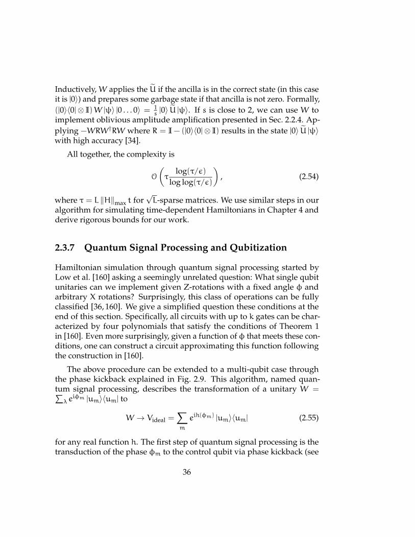
Inductively, W applies the U if the ancilla is in the correct state (in this caseit is |0〉) and prepares some garbage state if that ancilla is not zero. Formally,(|0〉〈0|⊗ I)W |ψ〉 |0 . . . 0〉 = 1
s |0〉 U |ψ〉. If s is close to 2, we can use W toimplement oblivious amplitude amplification presented in Sec. 2.2.4. Ap-plying −WRW†RW where R = I − (|0〉〈0|⊗ I) results in the state |0〉 U |ψ〉with high accuracy [34].
All together, the complexity is
O
(τ
log(τ/ε)log log(τ/ε)
), (2.54)
where τ = L ‖H‖max t for√L-sparse matrices. We use similar steps in our
algorithm for simulating time-dependent Hamiltonians in Chapter 4 andderive rigorous bounds for our work.
2.3.7 Quantum Signal Processing and Qubitization
Hamiltonian simulation through quantum signal processing started byLow et al. [160] asking a seemingly unrelated question: What single qubitunitaries can we implement given Z-rotations with a fixed angle φ andarbitrary X rotations? Surprisingly, this class of operations can be fullyclassified [36, 160]. We give a simplified question these conditions at theend of this section. Specifically, all circuits with up to k gates can be char-acterized by four polynomials that satisfy the conditions of Theorem 1in [160]. Even more surprisingly, given a function of φ that meets these con-ditions, one can construct a circuit approximating this function followingthe construction in [160].
The above procedure can be extended to a multi-qubit case throughthe phase kickback explained in Fig. 2.9. This algorithm, named quan-tum signal processing, describes the transformation of a unitary W =∑λ eiφm |um〉〈um| to
W → Videal =∑m
eih(φm) |um〉〈um| (2.55)
for any real function h. The first step of quantum signal processing is thetransduction of the phase φm to the control qubit via phase kickback (see
36

• = Rz(φm)
|ψm〉 U |ψm〉
Figure 2.9: Application of a controlled unitary acting on an eigenstate actsas a rotation on the control qubit. Let |ψm〉 be an eigenstate of U associ-ated with eigenvalue eiφm . Applying the circuit above on an initial state(α |0〉+β |1〉) |ψm〉 results in
(α |0〉+ eiφmβ |1〉
)|ψm〉. This is equivalent to
applying Rz(φm) =(
1 00 eiφm
)on the first qubit.
Fig. 2.9). Then, single qubit rotations are used to synthesize the desiredfunction as in the above control problem.
Quantum signal processing can be used together with a quantum walkoracle [27, 31]. Recall that the quantum walk operator has eigenvalues±e±i arcsinφm where φm is an eigenvalue of the Hamiltonian. Using thefunction h(θ) = −τ sin (θ) gives the proper time evolution. This functioncan be approximated by the Jacobi-Anger expansion in a manner similarto [31]. Importantly, Jacobi-Anger results in an achievable transformation(satisfying the criteria in [160]) and converges exponentially fast whichgives logarithmic scaling in error. In their next work, Low and Chuang [137]presented qubitization. Qubitization allows one to use quantum signalprocessing beyond the limitations of the signal oracle. Given access to theHamiltonian as H = 〈G|U |G〉 (see Subsection 2.3.1), one can construct a“qubiterate” to compute powers of H [137]. The name qubitization refersto decomposition into 2-dimensional invariant subspaces isomorphic toqubits. Qubitization allows one to combine quantum signal processingwith LCU methods and other techniques.
Gilyen et al. [36] later simplified and generalized these methods to atechnique called quantum singular value transformation (QSVT). We nowstate their version of quantum signal processing:
37
Theorem 4 (Quantum Signal Processing [36])Let k ∈ N; there exists Θ = θ0, θ1, . . . , θk ∈ Rk+1 such that for all x ∈ [−1, 1]:
eiθ0σz
k∏j=1
(W(x)eiθjσz
)=
[P(x) iQ(x)
√1 − x2
iQ(x)∗√
1 − x2 P∗(x)
]
where
W(x) =
[x i
√1 − x2
i√
1 − x2 x
]= ei arccos (x)σz
if and only if P,Q ∈ C[x] such that
• deg(P) 6 k and deg(Q) 6 k− 1
• P has parity (k mod 2) and Q has parity (k− 1 mod 2)
• ∀x ∈ [−1, 1] : |P(x)|2 + (1 − x2)|Q(x)|2 = 1
Simply put, Theorem 4 (Theorem 3 in [36]) states the conditions on thepolynomials that can be implemented through quantum signal processingcircuits. The proof of this theorem is constructive, giving an algorithmfor computing the angles from polynomials. In addition, if P or Q are notknown entirely, they can be completed following the proofs of Theorems3-5 of [36].
2.3.8 Generalization of the Hamiltonian Simulation Prob-lem
In the last subsection of the Background, we discuss several lines of researchclosely related to Hamiltonian simulation but extend it in various ways.
The first generalization is using a Hamiltonian that depends on time.Techniques for simulating time-dependent Hamiltonians based on theLie-Trotter-Suzuki decomposition were developed in [161–163], but thecomplexity scales polynomially with the error. Poulin et al. [163] gave analgorithm whose quantum complexity does not depend on the derivativesof the Hamiltonian because of their use of Monte Carlo integration.
38

More recent advances providing complexity logarithmic in the error[34,135] mention that their techniques can be generalized to time-dependentscenarios, but do not analyze this case. The most recent algorithms [35,137]are not directly applicable to the time-dependent case. Here we presentan explicit algorithm for simulating time-dependent Hamiltonians withcomplexity logarithmic in the allowable error, matching the complexity ofthe algorithms for the time-independent case in [34, 135], though not thosein [35, 137]. Low and Wiebe [37] independently achieved similar results.
Figure 2.10: The continuous-time evolution is discretized into shorttimesteps. The state in each step is then evolved with a time-independentHamiltonian.
Another avenue of research is the simulation of open quantum systems.An open quantum system can always be embedded into a closed one as aconsequence of Stinespring dilation [164]. As such, Hamiltonian simulationtechniques can also be used for the evolution of an open quantum system.However, extending a quantum system according to Stinespring dilation isprohibitively costly for practical simulations.
If the open system is Markovian, it is possible to simulate the LinblandMaster equation directly. Kliesch et al. [165] laid the basis for simulation ofMarkovian systems by showing that it can be simulated with complexitypolynomial in the evolution time and polylogarithmic in the dimension ifthe Lindbladian is k-local (see [165] for a formal definition) using Trotteri-zation. Childs and Li [166] extended this algorithm to sparse Lindbladians.Recently, Cleve and Wang proposed an algorithm logarithmic in inverseerror [167], extending LCU techniques to Markovian dynamics.
39

3Quantum Sort and Shuffle
“The order that our mind imagines is like a net,or like a ladder, built to attain something. Butafterward you must throw the ladder away,because you discover that, even if it was useful, itwas meaningless.”
Umberto Eco, The Name of the Rose
Randomness is an essential resource for many classical algorithms usedeverywhere from casinos to traffic route optimization. An example of acommon randomized subroutine is a shuffle. Given objects marked 1 to k,the shuffle produces a sequence of these objects uniformly at random.
In this section, we present a quantum version of the above task: preparean equal superposition of all permutations of k objects efficiently. Creatinga superposition is a natural extension of a shuffle because measurement inthe computational basis would reproduce an outcome of a classical shuffle.Note that we are strictly concerned by permutations without repetitions.
We present two different approaches to a quantum shuffle. The first oneis a quantization of a classical algorithm, the Fisher-Yates (FY) shuffle. The
40

second one approaches shuffle as the opposite of a sort. Indeed, if the origi-nal list of items is sorted, a sort can be seen as reverting the application of ashuffle. We extend classical sorting algorithms to the quantum frameworkby providing a reversible version with no asymptotic overhead.
Clearly, neither sort nor shuffle is reversible. We define shuffle as anoperation that takes a list in increasing order and outputs a symmetricsuperposition. A sort is then the inverse operation to the shuffle in thesense that a uniform superposition over possible permutations can besorted in increasing order.
This chapter is based on the paper Improved techniques for preparingeigenstates of fermionic Hamiltonians [2] which includes sort and shuffle assubroutines. I participated in the discussion, contributed with ideas, andwas involved in the writing process. Since I was primarily engaged inimproving antisymmetrization procedure utilizing a quantum sort or ashuffle, I decided to focus this chapter only on these techniques. My maincontributions were optimizing the algorithm for logarithmic depth and de-composing the components into elementary gates. Section 3.5 explains howone can use a sort or a shuffle in quantum chemistry as well as additionalapplications of our work. For instance, the algorithm in Chapter 4 uses thequantum sort as a subroutine.
3.1 How to Shuffle a Deck of Cards
Consider the following problem. We are given m cards, for simplicitylabeled from 1 tom. We want to shuffle them, i.e., output any ordering ofthe cards with equal probability. What random swaps should we performto shuffle the cards efficiently?
Intuitively, we could pick random pairs of cards and swap them, but wewould need to perform much more than n swaps to guarantee a genuinelyrandom permutation as can be seen in Fig. 3.1. Another strategy wouldbe to pick the first card deterministically and exchange its place with arandom card. Unfortunately, a naive approach based on this strategy doesnot produce uniform probabilities for all permutations.
A successful algorithm that requiresm swaps ensures that each card isdeterministically chosen only once. Note that a card can be swapped with
41
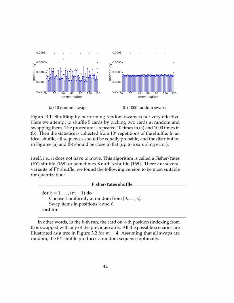
0 20 40 60 80 100 120permutation
0.0075
0.0080
0.0085
0.0090
0.0095
pro
babili
ty
(a) 10 random swaps
0 20 40 60 80 100 120permutation
0.0075
0.0080
0.0085
0.0090
0.0095
pro
babili
ty(b) 1000 random swaps
Figure 3.1: Shuffling by performing random swaps is not very effective.Here we attempt to shuffle 5 cards by picking two cards at random andswapping them. The procedure is repeated 10 times in (a) and 1000 times in(b). Then the statistics is collected from 107 repetitions of the shuffle. In anideal shuffle, all sequences should be equally probable, and the distributionin Figures (a) and (b) should be close to flat (up to a sampling error).
itself, i.e., it does not have to move. This algorithm is called a Fisher-Yates(FY) shuffle [168] or sometimes Knuth’s shuffle [169]. There are severalvariants of FY shuffle; we found the following version to be most suitablefor quantization:
Fisher-Yates shuffle
for k = 1, . . . , (m− 1) doChoose ` uniformly at random from 0, . . . ,k.Swap items in positions k and `.
end for
In other words, in the k-th run, the card on k-th position (indexing from0) is swapped with any of the previous cards. All the possible scenarios areillustrated as a tree in Figure 3.2 for m = 4. Assuming that all swaps arerandom, the FY shuffle produces a random sequence optimally.
42

1 4 6 71 4 7 61 7 6 47 4 6 11 6 4 71 6 7 41 7 4 6
1 4 6 7
7 6 4 16 4 1 76 4 7 16 7 1 4
4 1 64 1 6 74 1 7 64 7 6 17 1 6 2
1 6 4 7
4 1 7
4 1 6 7
4 6 1 74 6 7 14 7 1 6
6 1 46 1 4 76 1 7 46 7 4 17 1 4 6
4 6 1
6 1 4 7
1 4 6 7
4 1 6 7
1 4 6 7
k=3k=2k=1
76
77
Figure 3.2: A tree diagram for the FY shuffle demonstrates all the movesthat the algorithm can make. The blue boxes identify the array entries thathave been swapped at each stage of the shuffle. In the first step, the item“2” is moved, in the next one item “3” and item “4” is moved last. Note thatthe blue boxes also label the largest value in the array truncated to positionk.
3.2 Quantum Approach to a Shuffle
The FY algorithm presented above is not a unitary transformation and assuch, cannot be directly implemented on a quantum computer. Instead,we propose an algorithm that prepares a uniform superposition of allsequences, analogously to a classical shuffle.
Here we present our algorithm that implements a shuffle in superposi-
43

tion, i.e. performs the transformation
|r1 · · · rm〉 7→∑σ∈Sm
|σ (r1, · · · , rm)〉 , (3.1)
where σ iterates over possible permutations. Note that the choice of thestate is not unique; adding arbitrary phases eiφσ1 to the states |σ (r1, · · · , rm)〉would still fall within the definition of a quantum shuffle. In particular, thetransformation needed in [2] for fermionic state preparation was
|r1 · · · rm〉 7→∑σ∈Sm
(−1)π(σ) |σ (r1, · · · , rm)〉 (3.2)
where π(σ) is the parity of the permutation σ, and we require for the initialstate that rp < rp+1 (necessary for this procedure to be unitary). This meansthat we are solving a restricted version of the problem where the input isalways sorted in increasing order.
Although we describe the procedure for a single input |r1 · · · rm〉, ouralgorithm may be applied to any superposition of such states. We assumethat there are no repetitions among the shuffled items (this assumptionholds for fermions in the application of the shuffle in [2]) and the arraystarts ordered.
We first present a quantum extension of FY shuffle. Unfortunately,its complexity is worse than that of its classical counterpart. Then weshow an alternative algorithm utilizing sorting. As a part of the algorithm,we develop a quantum approach to sorting based on sorting networksand synthesize all the components down to elementary gates. This workpresents an exponential improvement in depth compared to the prior state-of-art [170].
3.3 Preparing a Uniform Superposition With theQuantum FY Shuffle
In this Section, we present a quantum version of FY shuffle that givesan intuitive approach to antisymmetrization. Assuming that we need to
1Of course, some functions φσ can be difficult to implement
44

shuffle m numbers between 0 and N− 1, the size- and depth-complexityare O(m2 logN).
Two key steps turn the FY shuffle into a quantum algorithm. First, ourquantum implementation of the shuffle replaces the random selection ofswaps with a superposition of all possible exchanges. Unfortunately, thisstep presents an overhead compared to the classical FY shuffle. To achievethis superposition, the random variable is replaced by an equal-weightsuperposition 1√
k+1
∑k`=0 |`〉 in an ancillary register (called choice).
Second, we must reset the choice register at the end of each step. Toaccomplish this, we introduce an additional index register, which initiallycontains the integers 0, . . . ,m − 1. We shuffle both the length-m input
register and the index register, and the simple form of index enables us toeasily reset choice. The resulting state of the joint input⊗ index registeris still highly entangled; however, provided input was initially sorted inascending order, we can disentangle index from input.
As we explained in our paper, the quantum FY shuffle consists 6 steps.The high level overview of FY shuffle is illustrated in Fig. 3.3, and Fig. 3.4provides additional detail. We now briefly review these steps and thenexplain each in detail.
1. Initialization. Prepare the choice register in the state |0〉. Prepare theindex register in the state |0, 1, . . . ,m− 1〉. Also set a classical variablek = 1.
2. Prepare choice. Transform the choice register as
|0〉 → 1√k+ 1
k∑`=0
|`〉 . (3.3)
3. Execute swap. Swap element k of input with the element specifiedby choice. Also swap element k of index with the element specifiedby choice. If preparing an antisymmetric superposition, apply a −1phase to the input register if a non-trivial swap was executed (i.e. ifchoice does not encode k).
4. Reset choice. For each ` = 1, . . . ,k, subtract ` from the choice registerif position ` in index is equal to k. The resulting state of choice is |0〉.
45

5. Repeat. Increment k by one. If k < m, go to Step 2. Otherwise,proceed to the next step.
6. Disentangle index from input. For each k 6= ` = 0, 1, . . . ,m − 1,subtract 1 from position ` of index if the element at position k ininput is greater than the element at position ` in input. The resultingstate of index is |0, 0, . . . , 0〉, which is disentangled from input.
|0〉⊗η
FY1
. . .
FYη−1
|0〉⊗m
|0〉⊗mdlogme / INIT . . .
DETANGLE
|0〉⊗mdlogme
input / . . . SYMM(input)
Figure 3.3: High-level view of the FY shuffle as it appeared in [2]. Theprocedure acts on registers labeled (top to bottom) choice, index and input.The first step block represents Initialization and the FYk blocks consist ofsteps Prepare choice, Execute swap and Reset choice, see Fig. 3.4, fork between 1 and m− 1. The last block aims to Disentangle index frominput.
After the DETANGLE procedure, the ancillary registers choice and index
are reset to their initial all-zero states and the input register has beensymmetrized. The structure of FY blocks is depicted in Fig. 3.4. Eachblock starts with the preparation operator Πk to choice, then we applyselected swaps between choice and index and between choice and input.We conclude each block by applying a phase conditioned on choice toinput, and resetting the choice register. These procedures are applied atotal of m− 1 times (for each of k = 1, . . . ,m− 1). Their gate counts andcircuits depths are then multiplied by (m− 1). Disentangling index andinput is the most expensive component, but it is executed only once, so itcontributes only an additive cost to the overall resource requirement.
46
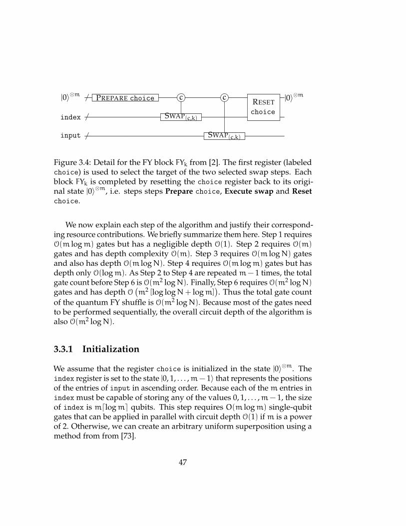
|0〉⊗m / PREPARE choice c cRESETchoice
|0〉⊗m
index / SWAP(c,k)
input / SWAP(c,k)
Figure 3.4: Detail for the FY block FYk from [2]. The first register (labeledchoice) is used to select the target of the two selected swap steps. Eachblock FYk is completed by resetting the choice register back to its origi-nal state |0〉⊗m, i.e. steps steps Prepare choice, Execute swap and Resetchoice.
We now explain each step of the algorithm and justify their correspond-ing resource contributions. We briefly summarize them here. Step 1 requiresO(m logm) gates but has a negligible depth O(1). Step 2 requires O(m)gates and has depth complexity O(m). Step 3 requires O(m logN) gatesand also has depth O(m logN). Step 4 requires O(m logm) gates but hasdepth only O(logm). As Step 2 to Step 4 are repeatedm− 1 times, the totalgate count before Step 6 is O(m2 logN). Finally, Step 6 requires O(m2 logN)gates and has depth O
(m2 [log logN+ logm]
). Thus the total gate count
of the quantum FY shuffle is O(m2 logN). Because most of the gates needto be performed sequentially, the overall circuit depth of the algorithm isalso O(m2 logN).
3.3.1 Initialization
We assume that the register choice is initialized in the state |0〉⊗m. Theindex register is set to the state |0, 1, . . . ,m− 1〉 that represents the positionsof the entries of input in ascending order. Because each of them entries inindex must be capable of storing any of the values 0, 1, . . . ,m− 1, the sizeof index is mdlogme qubits. This step requires O(m logm) single-qubitgates that can be applied in parallel with circuit depth O(1) ifm is a powerof 2. Otherwise, we can create an arbitrary uniform superposition using amethod from from [73].
47
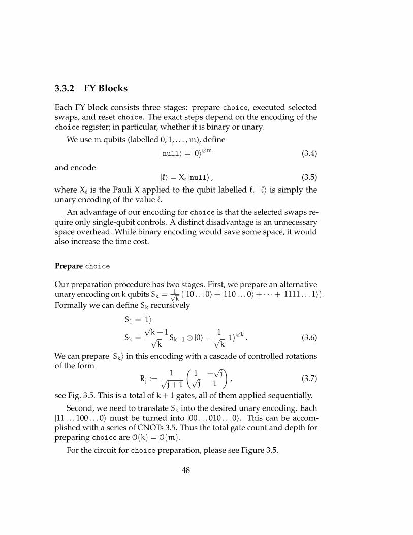
3.3.2 FY Blocks
Each FY block consists three stages: prepare choice, executed selectedswaps, and reset choice. The exact steps depend on the encoding of thechoice register; in particular, whether it is binary or unary.
We usem qubits (labelled 0, 1, . . . ,m), define
|null〉 = |0〉⊗m (3.4)
and encode|`〉 = X` |null〉 , (3.5)
where X` is the Pauli X applied to the qubit labelled `. |`〉 is simply theunary encoding of the value `.
An advantage of our encoding for choice is that the selected swaps re-quire only single-qubit controls. A distinct disadvantage is an unnecessaryspace overhead. While binary encoding would save some space, it wouldalso increase the time cost.
Prepare choice
Our preparation procedure has two stages. First, we prepare an alternativeunary encoding on k qubits Sk = 1√
k(|10 . . . 0〉+ |110 . . . 0〉+ · · ·+ |1111 . . . 1〉).
Formally we can define Sk recursively
S1 = |1〉
Sk =
√k− 1√kSk−1 ⊗ |0〉+ 1√
k|1〉⊗k . (3.6)
We can prepare |Sk〉 in this encoding with a cascade of controlled rotationsof the form
Rj :=1√j+ 1
(1 −
√j√
j 1
), (3.7)
see Fig. 3.5. This is a total of k+ 1 gates, all of them applied sequentially.
Second, we need to translate Sk into the desired unary encoding. Each|11 . . . 100 . . . 0〉 must be turned into |00 . . . 010 . . . 0〉. This can be accom-plished with a series of CNOTs 3.5. Thus the total gate count and depth forpreparing choice are O(k) = O(m).
For the circuit for choice preparation, please see Figure 3.5.
48

0 X . . .
1 Rk • . . . •2 Rk−1 . . . •...
. . .. . .
k − 1 . . . •k . . . R1 •
Figure 3.5: Circuit for preparing the choice register at the beginning ofblock FYk from [2]. See Eq. (3.7) for the definition of R`. First we prepareSk state (3.6) using a cascade of controlled rotations. Then we turn it into aunary encoding through a series of CNOTs.
Selected Swap
The next step is to implement the selected swap operation:
SELSWAPk :=
k−1∑c=0
|c〉〈c|⊗ SWAP(c,k), (3.8)
where the swapped states are either in the index or the input registersand controlled by the choice register. The unary encoding of c the choice
register allows for a simple implementation of SELSWAP; see Fig. 3.6.
Observe that only the first k+1 subregisters are involved of each choice,index and input. For each i = 0, 1, . . . ,k, index[i] is of size dlogmewhereasinput[i] is of size dlogNe. Hence, the circuit consists of kdlogme+kdlogNeordinary 3-qubit controlled-SWAP gates that for the most part must be ex-ecuted sequentially, see Fig. 3.6. This is the operation responsible for theoverhead compared to a classical swap. While the randomized FY algo-rithm requires only one (random) swap of registers, the coherent SELSWAPkhas complexity O (m logN) for both gate count and depth.
49
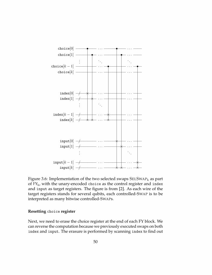
choice[0] • . . . • . . .
choice[1] • . . . • . . .
.... . .
. . .choice[k − 1] . . . • . . . •
choice[k] . . . . . .
index[0] / × . . . . . .
index[1] / × . . . . . ....
. . .
index[k − 1] / . . . × . . .
index[k] / × × . . . × . . .
input[0] / . . . × . . .
input[1] / . . . × . . ....
. . .
input[k − 1] / . . . . . . ×input[k] / . . . × × . . . ×
Figure 3.6: Implementation of the two selected swaps SELSWAPk as partof FYk, with the unary-encoded choice as the control register and index
and input as target registers. The figure is from [2]. As each wire of thetarget registers stands for several qubits, each controlled-SWAP is to beinterpreted as many bitwise controlled-SWAPs.
Resetting choice register
Next, we need to erase the choice register at the end of each FY block. Wecan reverse the computation because we previously executed swaps on bothindex and input. The erasure is performed by scanning index to find out
50
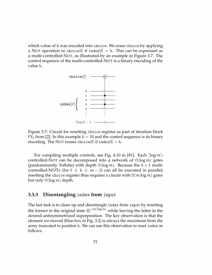
which value of kwas encoded into choice. We erase choice by applyinga NOT operation to choice[`] if index[`] = k. This can be expressed asa multi-controlled-NOT, as illustrated by an example in Figure 3.7. Thecontrol sequence of the multi-controlled-NOT is a binary encoding of thevalue k.
choice[`]
0
1 •2
index[`]
3 •4...
...
dlog ηe − 1
Figure 3.7: Circuit for resetting choice register as part of iteration blockFYk from [2]. In this example k = 10 and the control sequence is its binaryencoding. The NOT erases choice[`] if index[`] = k.
For compiling multiple controls, see Fig. 4.10 in [81]. Each dlogme-controlled-NOT can be decomposed into a network of O(logm) gates(predominantly Toffolis) with depth O(logm). Because the k+ 1 multi-controlled-NOTs (for ` 6 k 6 m − 1) can all be executed in parallel,resetting the choice register thus requires a circuit with O(m logm) gatesbut only O(logm) depth.
3.3.3 Disentangling index from input
The last task is to clean up and disentangle index from input by resettingthe former to the original state |0〉⊗mdlogme while leaving the latter in thedesired antisymmetrized superposition. The key observation is that theelement we moved (blue box in Fig. 3.2) is always the maximum from thearray truncated to position k. We can use this observation to reset index asfollows.
51
We compare the value carried by each of the m subregisters input[`](labeled by position index ` = 0, 1, . . . ,m− 1) with the value of each othersubregister input[` ′] (` ′ 6= `), thus requiring m(m − 1) comparisons intotal. Note that these subregisters of input have all size dlogNe. Each timethe value held in input[`] is larger than the value carried by any other ofthe remaining m− 1 subregisters input[` ′], we decrease the value of thecorresponding `th subregister index[`] of index by 1. If the value carried byinput[`] is smaller than input[` ′], we do not decrement the value of index[`].This way we identify the original position of the number currently encodedat input[`] at thus the value in index[`] subregister. After accomplishingall the m(m − 1) comparisons within the input register and controlleddecrements, we have reset the index register state to |0〉⊗mdlogme whileleaving the input register in the antisymmetrized superposition state.
The comparisons between the values of two subregisters of input (eachof size dlogNe) can be performed with O(logN) gates and O(log logN)depth using a quantum comparison from Section 3.4.2. The oracle’s outputis used to control the ‘decrement by 1’ operation, after which the oracle isused again to uncompute the ancilla holding its result.
Decrementing the value of the dlogme-sized index subregister index[`](for any ` = 0, 1, . . . ,m− 1) by the value 1 can be achieved by a circuitdepicted in Figure 3.8.
Each decrement consists of a total of dlogme multi-controlled-NOTs.Each multi-controlled-NOT involves n = dlogme− 1, . . . , 0 controls plusthe control on the qubit holding the result of the comparison. These gatescan be decomposed into O(n) Toffoli gates (see [81]), but the majority ofthe involved Toffoli gates for different values of n will effectively canceleach other out. The resulting cost is then O (logm) gates and no ancillaesince we can reuse qubits from choice register.
3.3.4 Complexity Analysis of the FY shuffle
Putting everything together, the overall circuit size for this step amounts toO (m(m− 1) [logN+ logm]) predominantly Toffoli gates, which can thenbe further decomposed into CNOTs and single-qubit gates (including Tgates) in well-known ways. Becausem 6 N, we thus report O(m2 logN) for
52

(a) (b)0 0
1 1
2 = 2
3 3
4 4
5 5
|0〉 • • • |0〉|0〉 • • • |0〉|0〉 • |0〉
Figure 3.8: Circuit implementing ‘decrement by 1’ operation, applied toindex[`] subregisters of size dlogme from [2]. (a) Example form = 64. (b)Decomposition into a network of O (logm) Toffoli gates using O (logm)ancillae.
the overall gate count for this step, while its circuit depth is O(m2 log logN+m2 logm).
3.4 Symmetrization Through Quantum Sorting
Our second approach to (anti)symmetrization uses a sorting algorithm.Classically, sorting is not used as a part of a shuffle, because the FY shuffleis more efficient. The situation is different for quantum algorithms, makingan approach utilizing a sort more appealing. Sadly, most well-knownclassical algorithms are not well-suited for quantization. Quicksort’s worstcase runtime, m2 applies every time if run in superposition. A standardrecursive application of merge sort requires a large space overhead. Otheralgorithms, for example, heapsort, implement operations whose positiondepends on values stored in the registers. This overhead is analogical
53

to selected swaps in FY shuffle. In this Section, we show that sortingnetworks are well-suited for quantum algorithms and give detailed circuitsto implement them.
Quantum sort can speed up the preparation of a symmetrization andantisymmetrization of sequences. Sorting for antisymmetrization wasoriginally proposed in [170], but has complexity O(m2 logN) and is notoptimized for depth.
The algorithm that we describe now has the complexity O(m logm logN)and depth O(logm log logN). We first review the four main steps and thenexplain them in detail:
1. Prepare seed. Let η > m2. In this step, we prepare an ancillaryregister called seed in an even superposition of all possible length-mstrings of the numbers 0, 1, . . . ,η − 1 in binary encoding. If η is apower of two, preparing seed consist of the Hadamard transform.
2. Sort seed. Sort seed using a quantum sorting network. This requires amodification of a sorting network that encoded the performed swapsin a second ancillary register called record. Comparing numbers isalso performed coherently and can be parallelized. There are severalknown sorting networks with polylogarithmic runtime, as we discussbelow.
3. Delete collisions from seed. At this point, we need to remove re-peated entries from seed. Due to the choice of η, repetitions arerare as a consequence of the birthday paradox. As we consider onlypermutations without repetition, we need to identify and delete the re-peats. We further prove that the resulting state of seed is disentangledfrom record, meaning seed can be discarded after this step.
4. Apply the reverse of the sort to target. Using the comparator valuesstored in record, we apply each step of the sorting network in reverseorder to the sorted array target. The resulting state of target is anevenly weighted superposition of each possible permutation of theoriginal values. If we wish to include a −1 phase for each permutation,we can apply a Z gate after each swap.
54
Step 4 is the key step for preparing a symmetric superposition. Havingprepared (in Step 1-Step 3) a record of the in-place swaps needed to sort asymmetrized, collision-free array, we undo each of these swaps in turn onthe sorted target. We demonstrate the algorithm on an example in Fig. 3.9.
In the next Section, we explain sorting networks and their implementa-tion on a quantum computer. Then, we show how to compare two numberscoherently, which is an elementary operation necessary in sorting. In thenext Subsection 3.4.3, we explain Step 3, Delete collisions. We concludethis section by connecting all the components and computing the complex-ity of our algorithm.
We employ a sorting network, a sorting method used in hardware,because sorting networks have comparisons and swaps at a fixed sequenceof locations.
3.4.1 Quantum Sorting Network
Sorting networks are logical circuits that consist of wires carrying valuesand comparator modules applied to pairs of wires, that compare valuesand swap them if they are not in the correct order, see Fig. 3.10. Theywere developed for sorting on a hardware level. Sorting networks aredata-oblivious, meaning that performed operations do not depend on theinput which makes them ideal for implementation in quantum computers.
Wires represent bit strings (integers stored in binary) in classical sortingnetworks and qubit strings in their quantum analogs. A classical compara-tor2 is a sort on two numbers. In other words, on an ordered pair of inputsA and B, a comparator implements the transformation
comparator ([A,B]) = [min(A,B), max(A,B)] , (3.9)
producing an ordered pair of A, B in increasing order. A quantum com-parator is its reversible version where we record whether the items werealready sorted (ancilla state |0〉) or the comparator needed to apply a swap(ancilla state |1〉); see Figure 3.11.
2The name comparator can be somehow misleading because this step involves aconditional step in addition to the comparision. Nevertheless, this is is the term used inthe literature.
55

Steps Prepare seed, Sort seed, and Delete collisions from seed
→ |0〉 |0〉 → |0〉 |0〉 |no swap〉 → ((((((((|0〉 |0〉 |no swap〉
→ |0〉 |1〉 → |0〉 |1〉 |no swap〉 → |0〉 |1〉 |no swap〉→ |0〉 |2〉 → |0〉 |2〉 |no swap〉 → |0〉 |2〉 |no swap〉→ |0〉 |3〉 → |0〉 |3〉 |no swap〉 → |0〉 |3〉 |no swap〉→ |1〉 |0〉 → |0〉 |1〉 | swap 〉 → |0〉 |1〉 | swap 〉→ |1〉 |1〉 → |1〉 |1〉 |no swap〉 → ((((((((
|1〉 |1〉 |no swap〉→ |1〉 |2〉 → |1〉 |2〉 |no swap〉 → |1〉 |2〉 |no swap〉→ |1〉 |3〉 → |1〉 |3〉 |no swap〉 → |1〉 |3〉 |no swap〉
|0〉 |0〉 → |2〉 |0〉 → |0〉 |2〉 | swap 〉 → |0〉 |2〉 | swap 〉→ |2〉 |1〉 → |1〉 |2〉 | swap 〉 → |1〉 |2〉 | swap 〉→ |2〉 |2〉 → |2〉 |2〉 |no swap〉 → ((((((((
|2〉 |2〉 |no swap〉→ |2〉 |3〉 → |2〉 |3〉 |no swap〉 → |2〉 |3〉 |no swap〉→ |3〉 |0〉 → |0〉 |3〉 | swap 〉 → |0〉 |3〉 | swap 〉→ |3〉 |1〉 → |1〉 |3〉 | swap 〉 → |1〉 |3〉 | swap 〉→ |3〉 |2〉 → |2〉 |3〉 | swap 〉 → |2〉 |3〉 | swap 〉→ |3〉 |3〉 → |3〉 |3〉 |no swap〉 → ((((((((
|3〉 |3〉 |no swap〉
The resulting state onseed and record.
(|0〉 |1〉+ |0〉 |2〉+ |0〉 |3〉+ |1〉 |2〉+ |1〉 |3〉+ |2〉 |3〉
)⊗(|swap〉+ |no swap〉
)
Step Apply the reverseof the sort to target.
(|4〉 |7〉
)(|swap〉+ |no swap〉
)→(|4〉 |7〉+ |7〉 |4〉
)|0〉
Figure 3.9: Example of the symmetrization by sorting for N = 4 and m = 2.Steps 1-3 operate only on ancillary registers seed and record and aim toprepare the desired superposition in record. In step 4 (last box), we userecord and a reverse sort to symmetrize the data stored in target.
The key feature of sorting networks is that the positions of comparatorsare predetermined. Therefore, they cannot depend on the inputs, unlike the
56
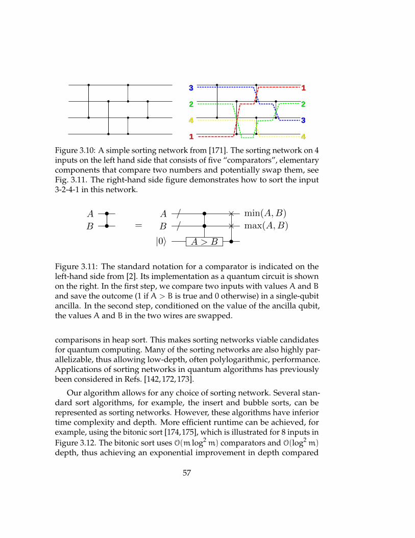
3
4
2
1
3
2
4
1
Figure 3.10: A simple sorting network from [171]. The sorting network on 4inputs on the left hand side that consists of five “comparators”, elementarycomponents that compare two numbers and potentially swap them, seeFig. 3.11. The right-hand side figure demonstrates how to sort the input3-2-4-1 in this network.
A • A / • × min(A,B)
B • = B / • × max(A,B)
|0〉 A > B •
Figure 3.11: The standard notation for a comparator is indicated on theleft-hand side from [2]. Its implementation as a quantum circuit is shownon the right. In the first step, we compare two inputs with values A and Band save the outcome (1 if A > B is true and 0 otherwise) in a single-qubitancilla. In the second step, conditioned on the value of the ancilla qubit,the values A and B in the two wires are swapped.
comparisons in heap sort. This makes sorting networks viable candidatesfor quantum computing. Many of the sorting networks are also highly par-allelizable, thus allowing low-depth, often polylogarithmic, performance.Applications of sorting networks in quantum algorithms has previouslybeen considered in Refs. [142, 172, 173].
Our algorithm allows for any choice of sorting network. Several stan-dard sort algorithms, for example, the insert and bubble sorts, can berepresented as sorting networks. However, these algorithms have inferiortime complexity and depth. More efficient runtime can be achieved, forexample, using the bitonic sort [174,175], which is illustrated for 8 inputs inFigure 3.12. The bitonic sort uses O(m log2m) comparators and O(log2m)depth, thus achieving an exponential improvement in depth compared
57

to conventional sorting techniques. Similar performance can be obtainedusing an odd-even mergesort [174].
• • • • • •• • • • • •• • • • • •• • • • • •• • • • • •• • • • • •• • • • • •• • • • • •
Figure 3.12: Example of a classical bitonic sort on 8 inputs from [2]. Com-parators in each dashed box can be applied in parallel for depth reduction.A quantum version of of the bitonic sort uses the same order of swaps withcomparators defined in Fig. 3.11.
The asymptotically best sorting networks have depth O(logm) andcomplexity O(m logm), though there is a large constant which means theyare less efficient for realistic m [176, 177]. There is also a sorting networkwith O(m logm) complexity with a better multiplicative constant [178],though its depth is O(m logm) (so it is not logarithmic).
For a small number of inputs to be sorted (up to m = 20), very tightbounds have been derived for optimized circuit depth as well as the overallnumber of comparators. Knuth [169] and later Codish et al. [179] gavenetworks for sorting up to 17 numbers that were later shown to be optimalin depth, and up to m 6 10 also optimal in the number of comparators.Optimizations for up to 20 inputs have recently been achieved, see Table 1in [179]. For illustration, the best known sorting networks for 20 numbersrequire depth 11 and 92 comparators, with lower bounds reported as 10and 73 respectively. More extensive sorting networks can be built up byan in-place merging of smaller sorting networks, but the construction issub-optimal.
Assume that a quantum sorting network hasm wires, where each wirerepresents a quantum register with d qubits (i.e., d = logN). We can obtainthe resource requirements for a quantum sort by taking a (classical) sortingnetwork and multiplying its resources in terms of comparators by those
58

needed for a quantum comparator. A quantum comparator consists of aprocedure for comparing two numbers explained in Section 3.4.2 and acontrolled swap on registers of size d, see Fig. 3.11.
3.4.2 Quantum Comparator
Here we describe how to reversibly implement the comparison of the valueheld in one register with the value carried by a second equally-sized register,and store the result (larger or not) in a single-qubit ancilla.
We need to use it for implementing the comparator modules of quantumsorting networks as well as in our antisymmetrization approach based onthe quantum FY shuffle. We first explain a straightforward method forcomparison with depth linear in the length of the involved registers. In thesecond step, we then convert this prototype into an algorithm with depthlogarithmic in the register length using a divide and conquer approach.
Let us compare two values A and B encoded as binaries in two equallysized registers, A and B. Intuitively, we can compare the registers in a bit-by-bit fashion, starting with their most significant bits and going down to theirleast significant bits. At the very first occurrence of an i such that A[i] 6= B[i],i.e., either A[i] = 1 and B[i] = 0 or A[i] = 0 and B[i] = 1, we know that A > Bin the first case and A < B in the second case. If A[i] = B[i] for all i, thenA = B.
If we are performing this comparison in superposition, we no longerhave the option of stopping once we found the point of difference. Hence,we employ two ancillary registers denoted A ′ and B ′, that each consist ofd qubits initialized |0〉⊗d. These registers will encode the results of thecomparison. All the bitwise comparisons except for the first one will beconditioned on the values stored in A ′ and B ′. Once we found the mostsignificant bit where A[i] 6= B[i], we flip the bit into 1 in A ′ if A > B or flipthe bit into 1 in B ′ if B > A. This means that the results of all remainingcomparisons is insignificant and should not be recorded. Instead, we carrythe result of the comparison of the most significant bits all the way to theleast significant bit and use it for reading the result.
We illustrate the naive comparison protocol on an example in Table 3.1.While this algorithm works, it has the drawback that the bitwise compari-
59

Register i=0 i=1 i=2 i=3 i=4 i=5 i=6 i=7 i=8A 0 1 0 0 1 0 1 0 1B 0 1 0 0 0 1 1 1 0A ′ 0 0 0 0 1 1 1 1 1B ′ 0 0 0 0 0 0 0 0 0
Table 3.1: Example illustrating the idea of reversible bitwise comparison.The index i labels the bits of the registers. At i = 0 we compare the mostsignificant bits A[0] and B[0], and write 1 into ancilla A ′[0] if A[0] > B[0],or write 1 into ancilla B ′[0] if A[0] < B[0]. In our example, the ancillasremain as 0. While both A ′[i− 1] and B ′[i− 1] are zero, we keep comparingthe numbers bit by bit encoding the result into A ′[i] and B ′[i]. The firstoccurrence of A[i] 6= B[i] is for i = 4, at which stage the value of ancilla A ′[4]is switched to 1, as A[4] > B[4]. For the remaining steps, the remaining bitsof A and B will not be compared anymore. Instead, in each step we flipeach remaining bit of A ′ to 1, whereas all bits of B ′ remain 0. Thus, the lastbit of A ′ will be 1 while B ′[8] is 0, implying A > B.
son is conducted sequentially, which results in circuit-depth scaling O(d). Italso uses more ancilla qubits than necessary.
We can reduce the number of ancillae and the depth of the algorithmwith a divide-and-conquer approach. Let us split the register A into twoparts: A1 consisting of the first approximately d/2 bits and A2 consisting ofthe remaining approximately d/2 bits. Split register B in the very same wayinto subregisters B1 and B2. We can then determine which number is larger(or whether both are equal) for each pair (A1,B1) and (A2,B2) separatelyin parallel (using an unspecified method) and record the results of the twocomparisons in ancilla registers (A ′1, B ′1), (A
′2, B ′2). The least significant bits
of these four ancilla registers can be then used to deduce whether A > Bor A < B or A = B with just a single bitwise comparison. Thus, we effec-tively halved the depth by dividing the problem into smaller problems andmerging them afterward. This approach can be also be used for comparingsubregisters, giving a recursive algorithm. We now explain its bottom-upimplementation.
First, slice A and B into pairs of bits – the first slice contains A[0] andA[1], the second slice consists of A[2] and A[3], etc., and in the very same
60
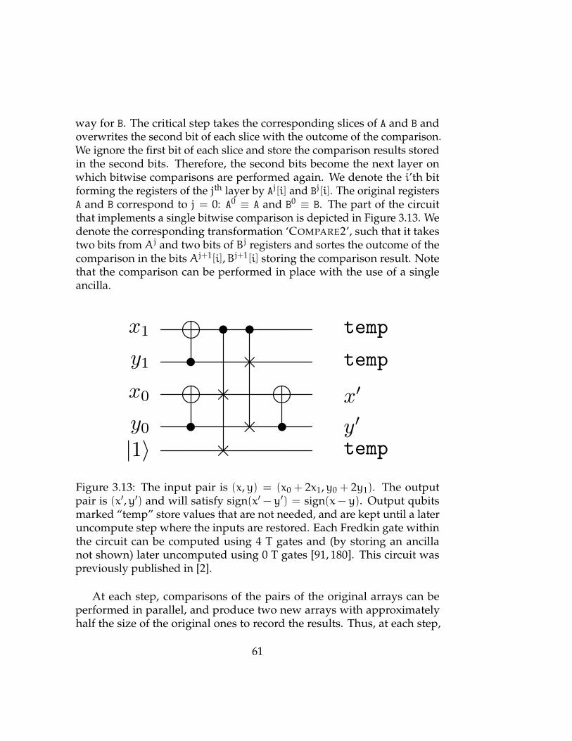
way for B. The critical step takes the corresponding slices of A and B andoverwrites the second bit of each slice with the outcome of the comparison.We ignore the first bit of each slice and store the comparison results storedin the second bits. Therefore, the second bits become the next layer onwhich bitwise comparisons are performed again. We denote the i’th bitforming the registers of the jth layer by Aj[i] and Bj[i]. The original registersA and B correspond to j = 0: A0 ≡ A and B0 ≡ B. The part of the circuitthat implements a single bitwise comparison is depicted in Figure 3.13. Wedenote the corresponding transformation ‘COMPARE2’, such that it takestwo bits from Aj and two bits of Bj registers and sortes the outcome of thecomparison in the bits Aj+1[i],Bj+1[i] storing the comparison result. Notethat the comparison can be performed in place with the use of a singleancilla.
x1 • • temp
y1 • × temp
x0 × x′
y0 • × • y′
|1〉 × temp
Figure 3.13: The input pair is (x,y) = (x0 + 2x1,y0 + 2y1). The outputpair is (x′,y′) and will satisfy sign(x′ − y′) = sign(x− y). Output qubitsmarked “temp” store values that are not needed, and are kept until a lateruncompute step where the inputs are restored. Each Fredkin gate withinthe circuit can be computed using 4 T gates and (by storing an ancillanot shown) later uncomputed using 0 T gates [91, 180]. This circuit waspreviously published in [2].
At each step, comparisons of the pairs of the original arrays can beperformed in parallel, and produce two new arrays with approximatelyhalf the size of the original ones to record the results. Thus, at each step,
61

we approximately halve the size of the problem, while using a constantdepth for computing the results. The basic idea is illustrated in Figure 3.14.This procedure is repeated for dlogde steps until registers Afin := Adlogde andBfin := Bdlogde both of size 1 have been prepared.
The parallelized algorithm is perfectly suited for comparing arrayswhose length d is a power of 2. If d is not a power of 2, we can eitherpad A and B with 0s prior to their most significant bits without alteringthe result, or introduce comparison of single bits (using only the first twogates from the circuit in Figure 3.13 with targets on Aj+1 and Bj+1 registersrespectively).
Formally, we can express our comparison algorithm as follows, hereassuming d to be a power of 2:
Low-depth comparison
for j = 0, . . . , logd− 1 dofor i = 0, . . . , size(Aj)/2 − 1 do(
Aj+1[i],Bj+1[i])= COMPARE2(Aj[2i],Bj[2i],Aj[2i+ 1],Bj[2i+ 1])
end forend forreturn (Alogd−1[0],Blogd−1[0])
The key feature of this algorithm is the parallelization of all the op-erations of the inner loop. Since one application of COMPARE2 requiresonly constant depth and a constant number of operations, our comparisonalgorithm requires only depth O(logd).
The above-constructed comparison algorithm can be used to output aresult that distinguishes between A > B, A < B and A = B. Its reversibleexecution results in the ancillary single-qubit registers Afin and Bfin generatedin the very last step of the algorithm holding information about whichnumber is larger or whether they are equal. Indeed, Afin[0] = Bfin[0] impliesA = B, Afin[0] < Bfin[0] implies A < B, and Afin[0] > Bfin[0] implies A > B.The three cases are separated into three control qubits by using the circuitshown in Figure 3.15. These individual control qubits can be used to controlfurther conditional operations that depend on the result of the comparison.
After the output bit has been produced, we reverse the comparison
62
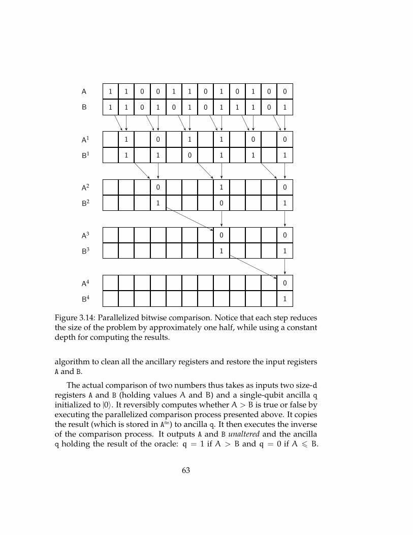
1 1 0 0 1 1 0 1 0 1 0 0
1 1 0 1 0 1 0 1 1 1 0 1
1 0 1 1 0 0
1 1 0 1 1 1
0 1 0
1 0 1
0 0
1 1
0
1
A
B
A1
B1
A2
B2
A3
B3
A4
B4
Figure 3.14: Parallelized bitwise comparison. Notice that each step reducesthe size of the problem by approximately one half, while using a constantdepth for computing the results.
algorithm to clean all the ancillary registers and restore the input registersA and B.
The actual comparison of two numbers thus takes as inputs two size-dregisters A and B (holding values A and B) and a single-qubit ancilla q
initialized to |0〉. It reversibly computes whether A > B is true or false byexecuting the parallelized comparison process presented above. It copiesthe result (which is stored in Afin) to ancilla q. It then executes the inverseof the comparison process. It outputs A and B unaltered and the ancillaq holding the result of the oracle: q = 1 if A > B and q = 0 if A 6 B.
63

x • x
y • • x=y
|0〉 • x<y
|0〉 x>y
Figure 3.15: A circuit that determines if two bits are equal, ascending, ordescending from [2]. When the comparison is no longer needed, the resultsare uncomputed by applying the circuit in reverse order.
As shown, this oracle has circuit size O(d) but depth only O(logd) and aT-count of 8d+O(1).
The second part of the comparator consists of conditional swaps on tworegisters of size d. Since all the single-bit swaps are conditioned on the sameancilla qubit, it may appear that these swaps should be applied sequentially,which would imply depth scaling O(d). However, the conditional swapscan also be parallelized by first copying the bit of the ancilla holding theresult of the comparison to additional ancillae initialized in |0〉 states. Suchan expansion of the result to d copies can be attained with a parallelizedarrangement of O(d) CNOTs but with circuit depth only O(logd). Aftercopying, all the d controlled elementary swaps can then be executed in par-allel (by using the additional ancillae) with circuit depth only O(1). Next,the d− 1 additional ancillae used for holding the copied result of compari-son are uncomputed again, by reversing the copying process. While thisprocedure requires O(d) ancillary space overhead, it optimizes the depth.The overall space overhead of the quantum comparator is also O(d).
Taking d = dlogNe (the largest registers used in Step 4 of our sort-based antisymmetrization algorithm), conducting the quantum bitonic sort,for instance, thus requires O(m log2(m) logN) elementary gates but onlyO(log2(m) log logN) circuit depth.
64

Similar scaling can be achieved using an algorithm from Draper etal. [181]. As presented, our work uses slightly fewer Toffoli gates andancillae compared to [181]. However, the number of CNOTs and overalldepth are larger.
3.4.3 Analysis of ‘Delete Collisions’ Step
In this Section, we explain how repeated items (collisions) can be deletedfrom seed. This step is non-deterministic and involves a measurement.We have to show that our algorithm is highly likely to succeed becausecollisions are relatively rare for a given set of parameters. If this part fails,we can restart the algorithm and repeat steps 1-3. We require that thechance of failure is at most 1
2 ; therefore, the expected number of runs ofsteps 1-3 is at most 2. Additionally, because we want to uncompute record
during the final step of our algorithm, we have to show that the resultingstate of seed is disentangled from record.
Let us first look at the state of seed after Step 1
1ηm/2
η−1∑`0,...,`m−1=0
|`0, . . . , `m−1〉 . (3.10)
The state (3.10) can be decomposed into a part with no repetitions andone when repetitions occur. Clearly, these two subspaces are mutuallyorthogonal.
To show that the probability of success is high, we need to compute thesupport of (3.10) on the subspace with no repetitions. This task is exactlyopposite to the birthday problem [182]; we want the likelihood of `i = `jfor any i 6= j to be small.
Comparing the number of permutations without and with repetitions(just as for the generalized birthday problem), we can show that the normof the projection onto the repetition-free subspace is
m!ηm
(η
m
). (3.11)
65
Using Proposition A.1 in [182], the probability of success is lowerbounded as
Pr(success) =m!ηm
(η
m
)> 1 −
m(m− 1)2η
, (3.12)
which is more than 1/2 for η > m2.
To detect the repetitions in our algorithm, we need to compare thevalues of `i in seed. It is advantageous to perform the comparisons inStep 3 after sorting the registers because then it is only necessary to checkadjacent entries. Sorting does not affect whether there are repetitions. Therepetition-free outcome can be achieved after fewer than two attempts onaverage. One can improve the success probability by using a larger η or byusing amplitude amplification.
We are left to show that seed is not entangled with record after Step3. After Step 1, the state of seed⊗ record projected to the repetition-freesubspace is proportional to∑
06`0<...<`m−1<η
∑σ∈Sm
|σ (`0, . . . , `m−1)〉seed |ι〉record . (3.13)
The register record will encode the performed permutation, in terms ofperformed swaps, applied to seed. At this stage, record is initialized to theidentity permutation denoted as ι.
In Step 2, we sorted seed by applying a series of swaps σ1, . . . ,σT whichwe recorded in record. Since the swaps were intentionally chosen to orderthe elements in seed, we effectively uncompute the initial permutation σ.Formally,
σT · · · σ1 = σ−1. (3.14)
Note that the repetitions-free subspace is closed under sorting. There-fore, we do not need to consider repeated elements in this analysis.
All together, Steps 1-2 transform seed⊗record projected on the repetition-free subspace as
∑06`0<...<`m−1<eta
∑σ∈Sm
|σ (`0, . . . , `m−1)〉seed |ι〉record (3.15)
→∑
06`0<...<`m−1<η
|`0, . . . , `m−1〉seed∑σ∈Sm
|σ1, . . . ,σT 〉record (3.16)
66

In Step 3, we can flag and eliminate repetitions which leaves us withthe state in Eq. (3.16). Notice that the states in registers seed and record
are not entangled. Since we only need the state in record, see Fig. 3.9, wecan safely discard seed.
3.4.4 Complexity Analysis of the Shuffle via Sorting
We now give the complexity of the shuffle via sorting by collecting the com-plexities of its components. Assuming we use an asymptotically optimalsorting network, the circuit depth for our algorithm is O(logm log logN)and the gate complexity is O(m logm logN). The dominant cost of thealgorithm comes from Step 2 and Step 4, each of which has O(m logm)comparators that can be parallelized to ensure the sorting network ex-ecutes only O(logm) comparator rounds. Each comparator for Step 4has a complexity of O(logN) and a depth of O(log logN), as we show inSec. 3.4.2. The comparators for Step 2 have complexity O(logm) and depthO(log logm), which is less because m < N. Thus Step 2 and Step 4 eachhave gate complexity O(m logm logN) and runtime O(logm log logN).
The other two steps in our algorithm have smaller cost. Step 1 has con-stant depth and O(m logm) complexity. Step 3 requires O(m) comparisonsbecause be only need to compare adjacent registers on seed after sorting.These comparisons can be parallelized over two rounds, with complexityO(m logm) and circuit depth O(log logm). Then the result for any of theregisters being equal is computed in a single qubit, which has complexityO(m) and depth O(logm). Thus the complexity of Step 3 is O(m logm)and the total circuit depth is O(logm). Thus, our algorithm has an expo-nential improvement in depth over the proposal in Refs. [170, 183]. We alsohave a quadratic improvement in gate complexity, which is O(m) for ouralgorithm but O(m2) for Refs. [170, 183].
The depth of our algorithm is likely optimal for symmetrization, atleast in terms of the m scaling. Symmetrization takes a single computa-tional basis state and generates a superposition ofm! computational basisstates. Each single-qubit operation can increase the number of states inthe superposition by at most a factor of two, and two-qubit operationscan increase the number of states in the superposition by at most a factorof four. Thus, the number of one- and two-qubit operations is at least
67

log2(m!) = O(m logm). In our algorithm, we need this number of opera-tions between the registers. If that is true in general, then m operations canbe parallelized, resulting in minimum depth O(logm).
Our quoted asymptotic runtime and gate complexity scalings assumethe use of sorting networks that are asymptotically optimal. However,these algorithms have a large constant overhead making it more practicalto use an odd-even mergesort, leading to depth O(log2m log logN). Notethat is possible to obtain complexity O(m logm logN) with a better scalingconstant using the sorting network of Ref. [178] but worse depth. Alltogether, we can summarize our results in the theorem below:
Theorem 5 (Quantum shuffle)Define a quantum shuffle as the transformation
|r1 · · · rm〉 →∑σ∈Sm
|σ (r1, · · · , rm)〉 , (3.17)
where 0 < r1 < r2 · · · < rm < N are encoded in binary and σ iterates over thepermutations. The quantum shuffle can be performed using O(m log2m logN)gates and depth O(logm log logN).
3.5 Applications
The need for a quantum shuffle arises in the state preparation problem inquantum chemistry with first quantization as outlined in Fig. 3.16.
State preparation is the first step for eigenstate (and particularly groundstate) preparation algorithms. The goal of this step is to prepare a state thathas a significant overlap with the ground state. The state is specified bylisting the orbital for each fermion. Note that we described the algorithm asworking on a state in the computational basis but a superposition of statesis also possible. We can index the orbitals as 0 toN1. Since the number oforbitals is typically much larger than the number of fermions m, we canperform the Delete collisions step correctly. Since it represents fermions, thestate must be completely antisymmetric (exchanging two fermions leads toa (−1) phase). As a result, no two fermions can occupy the same state.
68
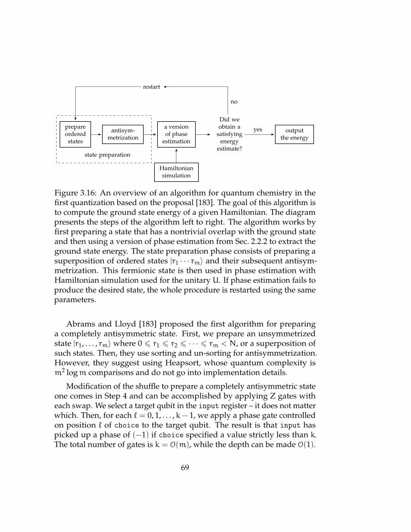
prepareordered
states
antisym-metrization
a versionof phase
estimation
Hamiltoniansimulation
Did weobtain a
satisfyingenergy
estimate?
outputthe energy
restart
no
yes
state preparation
Figure 3.16: An overview of an algorithm for quantum chemistry in thefirst quantization based on the proposal [183]. The goal of this algorithm isto compute the ground state energy of a given Hamiltonian. The diagrampresents the steps of the algorithm left to right. The algorithm works byfirst preparing a state that has a nontrivial overlap with the ground stateand then using a version of phase estimation from Sec. 2.2.2 to extract theground state energy. The state preparation phase consists of preparing asuperposition of ordered states |r1 · · · rm〉 and their subsequent antisym-metrization. This fermionic state is then used in phase estimation withHamiltonian simulation used for the unitary U. If phase estimation fails toproduce the desired state, the whole procedure is restarted using the sameparameters.
Abrams and Lloyd [183] proposed the first algorithm for preparinga completely antisymmetric state. First, we prepare an unsymmetrizedstate |r1, . . . , rm〉 where 0 6 r1 6 r2 6 · · · 6 rm < N, or a superposition ofsuch states. Then, they use sorting and un-sorting for antisymmetrization.However, they suggest using Heapsort, whose quantum complexity ism2 logm comparisons and do not go into implementation details.
Modification of the shuffle to prepare a completely antisymmetric stateone comes in Step 4 and can be accomplished by applying Z gates witheach swap. We select a target qubit in the input register – it does not matterwhich. Then, for each ` = 0, 1, . . . ,k− 1, we apply a phase gate controlledon position ` of choice to the target qubit. The result is that input haspicked up a phase of (−1) if choice specified a value strictly less than k.The total number of gates is k = O(m), while the depth can be made O(1).
69
Quantum sort and comparison has applications beyond symmetrizationand antisymmetrization. We utilized a quantum search in Chapter 4 toproduce a time ordering. A quantum comparison procedure introducedhere is essential for a black-box state preparation algorithm [116]. We useda similar technique in Chapter 4.
3.6 Conclusion
To conclude this Section, we have presented an algorithm for symmetriz-ing (or antisymmetrizing) a sorted, repetition-free quantum register. Wepropose two algorithms to accomplish this case. The first one is a quantumversion of FY shuffle. While FY shuffle is classically optimal, its quantumversion requires linear overhead to replace random swaps with preparingsuperposition over all possible swaps.
The second approach implements a shuffle by reversing a sort. Thechoice of a sort presents the dominant cost of this algorithm. We suggestusing sorting networks for sorting in quantum hardware and devise circuitsfor highly efficient sorting and comparison. The resulting asymptoticalgate count complexity and depth are, respectively, O(m logm logN) andO(logm log logN). This constitutes a polynomial improvement in the firstcase and exponential in the second case over previous work in Refs. [170,183]. As in Ref. [183], our algorithm can be used for state preparation of afermionic wavefunction in first quantization.
Our algorithm requires that the input is always sorted in increasing or-der. This assumption is easy to satisfy for the purposes for state preparationbut one may ask whether it is necessary. It is easy to see that our algorithmfails if the input is not ordered – we will not be able to clean record.
We can modify our sort based shuffling algorithm to allow for differenttypes of ordering provided that the input is still in strict order and wecan construct an alternative comparator for this order. Then we can applythe reverse sort in Step 4 with respect to this new order. We can easily(anti)symmetrize input in decreasing order with the same complexity butthe complexity with respect toNmight be different for different encodings.
70
4Simulation of Time-Dependent
Hamiltonians
“Every moment before this one depends on thisone.”
Jonathan Safran Foer (Extremely Loud andIncredibly Close)
This chapter is based on the paper [3] and significantly overlaps withits text. I contributed to all parts of the projects including the majority ofthe writing.
71
4.1 Unitary Evolution Under a Time-dependentHamiltonian
The Schrodinger equation
id
dt|ψ(t)〉 = H |ψ(t)〉 (4.1)
is one of the most famous equations in all of physics. It describes the timeevolution of a closed quantum system. We described in detail how tosolve it on a quantum computer in Section 2.3. The standard process ofanalytically solving (4.1) (albeit exactly possible only for a few special cases)is to find the eigenvalues Ej and eigenvectors
∣∣φj⟩
of the Hamiltonian andexpress the evolution for a time period T as
|ψ(T)〉 =∑j
〈φj|ψ(0)〉e−iEjt∣∣φj⟩
(4.2)
While solving the Schrodinger equation classically is almost always verydifficult, using a time-dependent Hamiltonian is even more complicated. Itis possible to find the instantaneous eigenvalues and the eigenvectors; theseare however different for each time and Eq. (4.2) no longer applies.
The formal solution of the evolution under a time-dependent Hamilto-nian can be written as
U(t0, t0 + T) = T exp
(−i
∫ t0+Tt0
dτH(τ)
), (4.3)
where T is the time ordering operator. Equation (4.3) can be interpreted asthe limit
U(t0, t0 + T) = limM→∞T
M−1∏n=0
exp−iT
MH
(t0 +
nT
M
). (4.4)
Solving the time-dependent Schrodinger equation analytically is inpractice almost always impossible. Dynamics of even a small system,say a 1
2-spin, can exhibit rich behavior that depends on the change of
72
the Hamiltonian. Many theoretical approaches have been developed toapproximate the evolution under a time-dependent Hamiltonian. Theadiabatic approximation [184, 185] can be used when the change of theHamiltonian is slowly varying.
Other approximations include the diabatic approximation and rotatingwave approximation. Nevertheless, the evolution under a general time-dependent Hamiltonian is a computationally difficult problem that can beonly solved through numerical simulation (for a small system), or simulatedon a quantum computer. Let us first define the problem of simulating timedependent Hamiltonians:
Problem 1 (The time-dependent Hamiltonian simulation problem)Let H be a time-dependent Hamiltonian that can be expressed as a time-de-pendent linear combination of unitaries as either H(t) =
∑L−1l=0 αl(t)Hl or
H(t) =∑L−1l=0 αlHl(t), where L is polylogarithmic in the dimension of the Hilbert
space of H. Given an initial state |ψ〉 at time t0, we aim to prepare
T exp
(−i
∫ t0+Tt0
dτH(τ)
)|ψ〉 (4.5)
for a finite time T , such that the maximum error in the final state, as quantified bythe trace distance, does not exceed ε.
4.2 Framework
4.2.1 Oracles
We consider two different representations of H(t): Hamiltonians that aregiven by a d-sparse time-dependent Hermitian matrix (scenario 1) andHamiltonians that are time-dependent linear combinations of some time-independent unitaries (scenario 2). While scenario 2 is already in the formrequired by Problem 1, we show that scenario 1 can be expressed as alinear combination of unitaries as well. The second scenario is also moregeneral than the first one but it can help us to benefit from an additionalstructure of the Hamiltonians. For example, Hamiltonians in quantum
73

chemistry, which is one of the main applications of quantum simulations,fall into the second scenario because they are commonly expressed as linearcombinations of tensor products of Pauli matrices.
Our algorithms for both scenarios rely on the ability to express thetime-dependent Hamiltonian as a linear combination of efficiently imple-mentable unitaries, similarly to [34]. Unlike [34], we need to include thetime-dependence in the decomposition. We can choose to add it either inthe coefficients or the unitaries. We show that either choice is possible andthe preferred approach depends on the structure of the Hamiltonian.
For d-sparse matrices we need compute the decomposition of the Hamil-tonian into a sum of unitaries. As such, it is more practical to take theunitaries to be time-dependent while making the coefficients in the decom-position constant. In contrast, for cases where the Hamiltonian is alreadygiven in the form of a sum of unitaries, we take the unitaries to be constant,and the time dependence is solely in the coefficients. This form is naturalfor applications such as quantum chemistry or adiabatic algorithms.
Let us now describe the oracles for both cases in more detail. In the firstscenario, access to a d-sparse Hamiltonian is provided through the oracles
Oloc |j, s〉 = |j,ν(j, s)〉 , (4.6)
Oval |t, i, j, z〉 =∣∣t, i, j, z⊕Hij(t)
⟩, (4.7)
where ⊕ represents a bitwise XOR. The above equations are a time-depen-dent analog of oracles (2.26) and (2.27) defined in Section 2.3. Here, ν(j, s)gives the position of the s’th element in row j of H(t) that may be nonzeroat any time. Note that the oracle Oloc does not depend on time but Oval
does. Oracle Oval yields the values of non-zero elements at each instant oftime.
Furthermore, we say that a time-dependent HamiltonianH(t) is d-sparseon the interval if the number of entries in any row or column that may benonzero at any time throughout the interval is at most d. This definition isdistinct from the maximum sparseness of the instantaneous HamiltoniansH(t), because some entries may go to zero while others become nonzero.(This definition of sparseness upper bounds the sparseness of instantaneousHamiltonians.)
74

4.2.2 Enabling Oblivious Amplitude Amplification
Our algorithm for d-sparse matrices builds on the unitary decomposition ofa Hermitian matrix into equal-sized 1-sparse self-inverse parts introducedin Lemma 4.3 in Ref. [135] that we explained in Sec. 2.3.4. The HamiltonianH(t) can be decomposed using the technique of Ref. [135] for any individualtime, giving
H(t) = γ
L−1∑`=0
H`(t), (4.8)
where the H`(t) are 1-sparse, unitary and Hermitian. The matrix entriesin H`(t) can be determined using O(1) queries according to Lemma 4.4 ofRef. [135]. The single coefficient γ is time-independent, and so is the sum ofcoefficients λ := Lγ in the decomposition. The value of γ should be chosenas (see Eq. (24) in [135])
γ ∈ Θ(ε/(d3T)) (4.9)
to give a contribution to the error that is O(ε). The unitary decomposition(4.8) can be computed with a number of Hamiltonians scaling as
L ∈ O(d2Hmax/γ
). (4.10)
Here we defined
Hmax = maxt∈[t0,t0+T ] ‖H(t)‖max . (4.11)
We also define a norm for the derivative of the Hamiltonian
Hmax = maxt∈[t0,t0+T ] ‖dH(t)/dt‖ , (4.12)
where ‖ · ‖ indicates the spectral norm and ‖ · ‖max the max-norm.
In the second scenario, we assume that the Hamiltonian already has theform of a unitary decomposition with time-dependent coefficients:
H(t) =
L−1∑`=0
α`(t)H` . (4.13)
In this scenario, the H` are all unitary and time-independent, while eachα`(t) is assumed to be a real-valued differentiable function with modulus
75

upper bounded by a known constant αmax > |α`(t)| for t ∈ [0, T ] and all` ∈ 0, . . . ,L− 1.
The condition α`(t) ∈ R can always be attained by decomposing anycomplex-valued coefficient into its real and imaginary parts and includingthe complex phase factor ±i in the associated unitary H`.
As in the first scenario, access to the Hamiltonian is provided throughoracles. We assume there is an efficient procedure to implement an oracleOunit that applies a single unitary from the decomposition (4.13) to thesystem state according to
Ounit |`〉a |Ψ〉s = |`〉aH` |Ψ〉s . (4.14)
The particular unitary H` is selected by the index value ` held in an ancillaregister state |`〉a. In one important example, the H` are composed of tensorproducts of Pauli matrices, in which case each such oracle query can beimplemented with O(L(n+ logL)) elementary gates; see [34]. However,we do not bind ourselves to a specific implementation and quantify thecomplexity only in terms of the number of oracle calls and the number ofadditional gates. Furthermore, we assume access to the time-dependentcoefficients through a coefficient oracle defined as
Ocoeff |`, t, z〉 = |`, t, z⊕α`(t)〉 . (4.15)
More precisely, the oracle returns a truncated version of the target coef-ficients as z⊕ α(ν)
` (t), where z is a ν-bit integer encoded into a ν-qubitregister, and α(ν)
` (t) := b2να`(t)c is a ν-bit fixed-point approximation to thereal value of α`(t).
The sum of the coefficients, λ(t) :=∑L−1`=0 α`(t), in the decomposition
(4.13) generally depends on time, which appears to be a problem for imple-menting oblivious amplitude amplification [34]. Successful implementationof oblivious amplitude amplification for a given interval requires that theintegral of λ(t) over that interval should be equal to ln 2. If we were toperform oblivious amplitude amplification on this decomposition directly,we would need to integrate λ(t) to find an appropriate length of the time in-terval, which would increase the computational complexity. How could weavoid this complication? In our construction, we alter the unitary decompo-sition (4.13) such that the sum of the new coefficients is time-independent
76
but corresponds to the same Hamiltonian. One option to create such adecomposition is
H(t) =
L−1∑`=0
αmax +α`(t)
2H` +
L−1∑`=0
αmax −α`(t)
2(−H`)
=
2L−1∑`=0
α`(t)H`, (4.16)
where
α`(t) :=
αmax+α`(t)
2 for ` = 0, . . . ,L− 1
αmax−α`−L(t)2 for ` = L, . . . , 2L− 1
(4.17)
H` :=
H` for ` = 0, . . . ,L− 1
−H`−L for ` = L, . . . , 2L− 1 .(4.18)
This new decomposition has 2L terms and the sum of its coefficients is byconstruction time-independent and equal to λ = Lαmax. This allows us tosatisfy the condition that is sufficient for achieving the oblivious amplitudeamplification procedure globally for the entire time interval [t0, t0 + T ].
4.3 Algorithm Overview
Our algorithm consists of the following steps summarized in the dia-gram 4.1.
4.3.1 Evolution Discretization
Our goal is to simulate the action of U in Eq. (4.3) within error ε. First,we divide the total simulation time T into r time segments of length T/r.Without loss of generality, we analyze the evolution induced within thefirst segment and set t0 = 0. The simulation of the evolution within
77
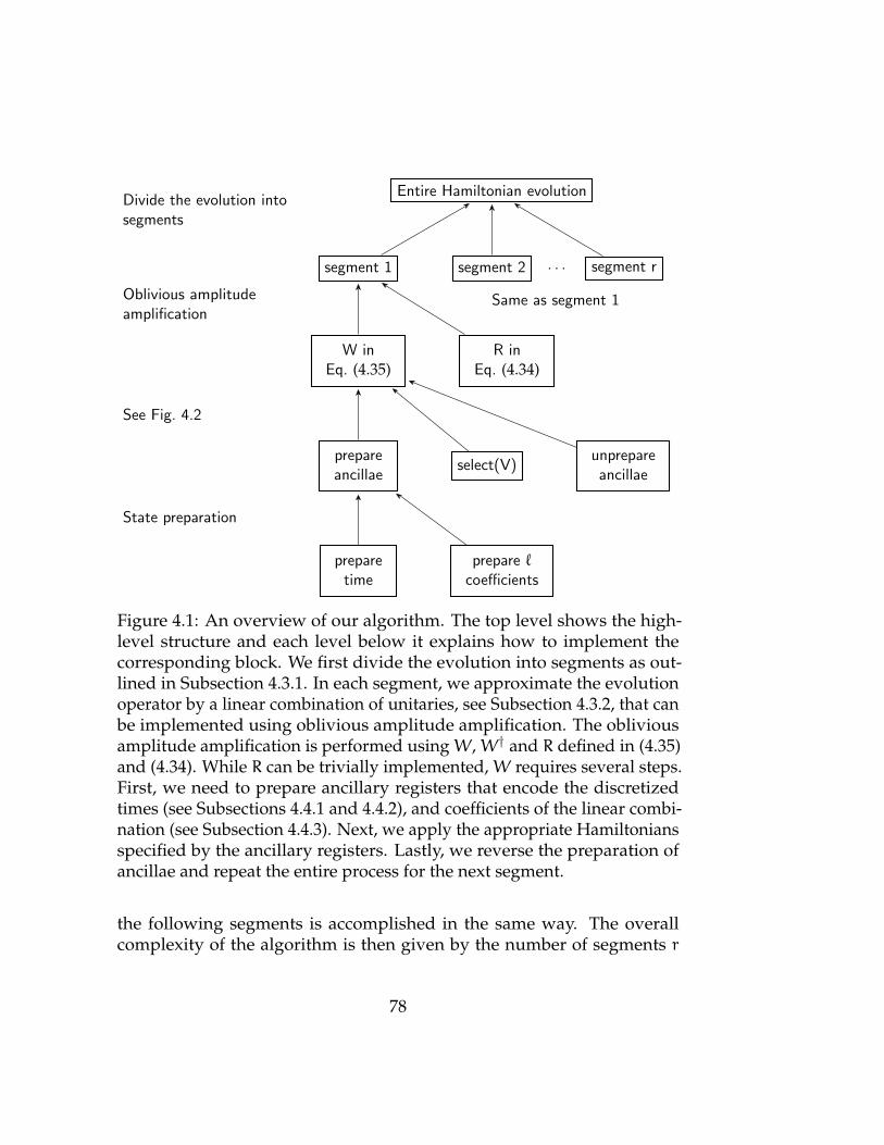
Entire Hamiltonian evolutionDivide the evolution intosegments
Oblivious amplitudeamplification
See Fig. 4.2
State preparation
Same as segment 1
segment 2segment 1 segment r
W inEq. (4.35)
R inEq. (4.34)
prepareancillae
select(V)unprepare
ancillae
preparetime
prepare `coefficients
. . .
Figure 4.1: An overview of our algorithm. The top level shows the high-level structure and each level below it explains how to implement thecorresponding block. We first divide the evolution into segments as out-lined in Subsection 4.3.1. In each segment, we approximate the evolutionoperator by a linear combination of unitaries, see Subsection 4.3.2, that canbe implemented using oblivious amplitude amplification. The obliviousamplitude amplification is performed usingW,W† and R defined in (4.35)and (4.34). While R can be trivially implemented,W requires several steps.First, we need to prepare ancillary registers that encode the discretizedtimes (see Subsections 4.4.1 and 4.4.2), and coefficients of the linear combi-nation (see Subsection 4.4.3). Next, we apply the appropriate Hamiltoniansspecified by the ancillary registers. Lastly, we reverse the preparation ofancillae and repeat the entire process for the next segment.
the following segments is accomplished in the same way. The overallcomplexity of the algorithm is then given by the number of segments r
78

times the cost of simulation for each segment. To upper bound the totalsimulation error by ε, we require the error of simulation for each segment tobe at most ε/r. By using an LCU technique, we can choose these segmentslonger than for Trotterization algorithms [161].
We need a set of qubits to encode the time over the entire time interval[0, T ]. It is convenient to take r to be a power of two, so there will be one setof qubits for the time that encodes the segment number, and another setof qubits that gives the time within the segment. The qubits encoding thesegment number are only changed by incrementing by 1 between segments,which gives complexity O(r log r). If it is not possible to take r as a powerof two, one can choose the last segment to be shorter and use an ancilla toperform oblivious amplitude amplification as in [135].
Let us now explain the key steps for decomposing the evolution into alinear combination of unitaries. We approximate the evolution within thefirst segment by a Dyson series up to K-th order:
U(0, T/r) ≈K∑k=0
(−i)k
k!T
∫T/r0dtH(tk) . . .H(t1) , (4.19)
where, for each k-th term in the Dyson series, T∫T/r
0 dt (·) represents inte-gration over a k-tuple of time variables (t1, . . . , tk) while keeping the timesordered: t1 6 t2 6 · · · 6 tk. It is straightforward to show that the error of
this approximation is O(HK+1
max(K+1)!
(Tr
)K+1)
.
Next, we discretize the integral over each time variable and approximateit by a sum withM terms. For convenience, we may choose to takeM to bea power of two. The time-dependent Hamiltonian is thereby approximatedby its values atM uniformly separated times jT
rM identified by an integerj ∈ 0, . . . ,M− 1. Approximating an integral with its Riemann sum yields
∫T/r0H(t)dt =
M−1∑j=0
∫ tj+1
tj
H(t)dt
≈M−1∑j=0
(T
rM
)H(tj), (4.20)
79
where t0 = 0 and tM = T/r. The incurred error can be then bounded by∑M−1j=0∫tj+1tj
∥∥H(t) −H(tj)∥∥dt .
In each of the time intervals [tj, tj+1] of length T/(rM) we have
‖H(t) −H(tj)‖ 6T
rMmaxz
∥∥∥∥dH(z)
dz
∥∥∥∥
6THmax
rM, (4.21)
where maxz indicates a maximum over that time interval.
Hence, the overall error of approximation in the integral over time T/r
is O((T/r)2Hmax
M
). That is, the error in the k = 1 term for U, and the error
for terms with k > 1, are higher order. The error for all r segments is thenO(T2HmaxrM
). We remark that a slightly tighter bound in terms of a time-
average of H(t) rather than in terms of Hmax is possible, as was achievedin [37]. Replacing all integrals by sums in expression (4.19) thus yields thefollowing approximation of the time-evolution operator within the firstsegment:
U :=
K∑k=0
(−iT/r)k
Mkk!
M−1∑j1,...,jk=0
TH(tjk) . . .H(tj1). (4.22)
The overall error of the obtained approximation is thus
‖U−U(0, T/r)‖ ∈ O
((HmaxT/r)
K+1
(K+ 1)!+
(T/r)2Hmax
M
). (4.23)
Provided that r > HmaxT , the overall error can be bounded by ε/r if wechoose
K ∈ Θ(
log (r/ε)
log log (r/ε)
)and M ∈ Θ
(T2Hmax
εr
). (4.24)
This expansion is analogous to truncated Taylor series explained inSection 2.3.6. Unlike in the time-independent algorithm [127] presented inSection 2.3.6, we need to preserve the correct order of Hamiltonians. We
80

achieve this by introducing an additional multi-qubit control register calledtime. This ancillary register is prepared in a certain superposition state(depending on which approach we take). We use this register to samplethe Hamiltonian at different times in superposition while respecting timeordering.
4.3.2 Linear Combination of Unitaries
Substituting the unitary decomposition, as defined in (4.8) or (4.16), into(4.22), the approximation of the time-evolution operator takes the formU =
∑j∈J βjVj. The index j is a multi-index and the coefficients βj comprise
information about both the time discretization and the unitary decomposi-tion weightings as well as the order k within the Taylor series. Explicitly,we define
β1
(k,`1,...,`k,j1,...,jk) :=(γ T/r)k
Mkk1!k2! . . . kσ!θk (j1, . . . , jk) , (4.25)
V 1
(k,`1,...,`k,j1,...,jk) := (−i)k H`k(tjk) . . .H`1(tj1) , (4.26)
when dealing with Hamiltonians given by a sparse matrix (scenario 1)giving decomposition (4.8), and
β2
(k,`1,...,`k,j1,...,jk) :=(T/r)k
Mkk1!k2! . . .kσ!θk (j1, . . . , jk) α`k(tjk) . . . α`1(tj1),
(4.27)
V 2
(k,`1,...,`k,j1,...,jk) := (−i)k H`k . . .H`1 , (4.28)
when dealing with scenario 2 Hamiltonians given by decomposition (4.13),where θk (j1, . . . , jk) = 1 if j1 6 j2 6 . . . 6 jk, and zero otherwise. Thequantity σ is the number of distinct values of j, and k1,k2, . . . ,kσ are thenumber of repetitions for each distinct value of j. That is, we have theindices j for the times sorted in ascending order, and we have multipliedby a factor of k!/(k1!k2! . . . kσ!) to take account of the number of unorderedsets of indices which give the same ordered set of indices. The multi-indexset J is defined as
J1 := (k, `1, . . . , `k, j1, . . . , jk) : k ∈ 0, . . . ,K, `1, . . . , `k ∈ 0, . . . ,L− 1,j1, . . . , jk ∈ 0, . . . ,M− 1, (4.29)
81
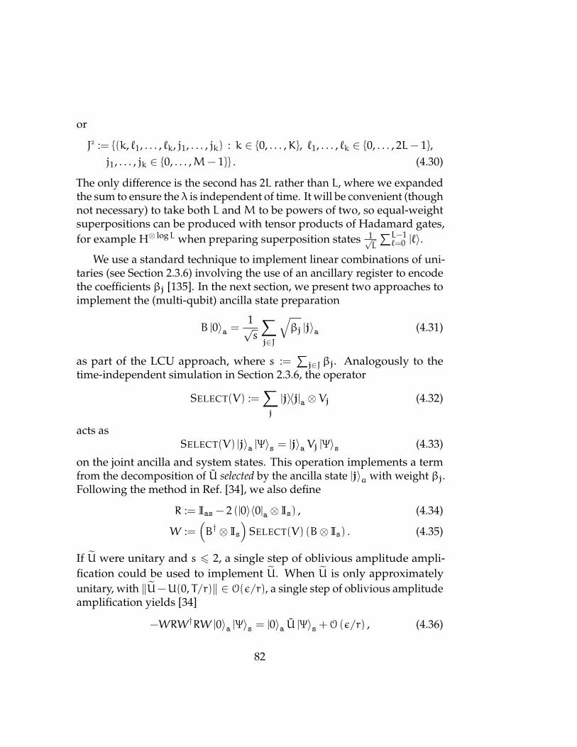
or
J2 := (k, `1, . . . , `k, j1, . . . , jk) : k ∈ 0, . . . ,K, `1, . . . , `k ∈ 0, . . . , 2L− 1,j1, . . . , jk ∈ 0, . . . ,M− 1 . (4.30)
The only difference is the second has 2L rather than L, where we expandedthe sum to ensure the λ is independent of time. It will be convenient (thoughnot necessary) to take both L andM to be powers of two, so equal-weightsuperpositions can be produced with tensor products of Hadamard gates,for example H⊗ logL when preparing superposition states 1√
L
∑L−1`=0 |`〉.
We use a standard technique to implement linear combinations of uni-taries (see Section 2.3.6) involving the use of an ancillary register to encodethe coefficients βj [135]. In the next section, we present two approaches toimplement the (multi-qubit) ancilla state preparation
B |0〉a =1√s
∑j∈J
√βj |j〉a (4.31)
as part of the LCU approach, where s :=∑
j∈J βj. Analogously to thetime-independent simulation in Section 2.3.6, the operator
SELECT(V) :=∑j
|j〉〈j|a ⊗ Vj (4.32)
acts asSELECT(V) |j〉a |Ψ〉s = |j〉a Vj |Ψ〉s (4.33)
on the joint ancilla and system states. This operation implements a termfrom the decomposition of U selected by the ancilla state |j〉a with weight βj.Following the method in Ref. [34], we also define
R := Ias − 2 (|0〉〈0|a ⊗ Is) , (4.34)
W :=(B† ⊗ Is
)SELECT(V) (B⊗ Is) . (4.35)
If U were unitary and s 6 2, a single step of oblivious amplitude ampli-fication could be used to implement U. When U is only approximatelyunitary, with ‖U−U(0, T/r)‖ ∈ O(ε/r), a single step of oblivious amplitudeamplification yields [34]
−WRW†RW |0〉a |Ψ〉s = |0〉a U |Ψ〉s +O (ε/r) , (4.36)
82
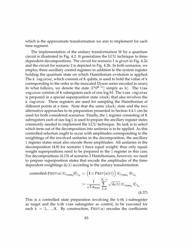
which is the approximate transformation we aim to implement for eachtime segment.
The implementation of the unitary transformation W by a quantumcircuit is illustrated in Fig. 4.2. It generalizes the LCU technique to time-dependent decompositions. The circuit for scenario 1 is given in Fig. 4.2aand the circuit for scenario 2 is depicted in Fig. 4.2b. In both scenarios, weemploy three auxiliary control registers in addition to the system registerholding the quantum state on which Hamiltonian evolution is applied.The k register, which consists of K qubits, is used to hold the value of kcorresponding to the order in the truncated Dyson series encoded in unary.In what follows, we denote the state
∣∣1k0K−k⟩
simply as |k〉. The time
register consists of K subregisters each of size logM. The time register
is prepared in a special superposition state |clock〉 that also involves thek register. These registers are used for sampling the Hamiltonian atdifferent points at a time. Note that the same |clock〉 state and the twoalternative approaches to its preparation presented in Section 4.4.1 can beused for both considered scenarios. Finally, the l register consisting of Ksubregisters each of size logL is used to prepare the ancillary register statescommonly needed to implement the LCU technique. Its task is to selectwhich term out of the decomposition into unitaries is to be applied. As thiscontrolled selection ought to occur with amplitudes corresponding to theweightings of the involved unitaries in the decomposition, the ancillaryl register states must also encode those amplitudes. All unitaries in thedecomposition (4.8) for scenario 1 have equal weight; thus only equal-weight superpositions need to be prepared in the l register in this case.For decompositions (4.13) of scenario 2 Hamiltonians, however, we needto prepare superposition states that encode the amplitudes of the time-dependent weightings α`(t) according to the unitary transformation
controlled-PREP(α) |t〉timek|0〉lk :=(
I⊗ PREP(α(t)
))|t〉timek |0〉lk
:=1√Lαmax
2L−1∑`=0
√α`(t) |t〉timek |`〉lk .
(4.37)
This is a controlled state preparation involving the k-th l-subregisteras target and the k-th time subregister as control, to be executed foreach k = 1, . . . ,K. By construction, PREP(α) encodes the coefficients
83

of the altered (but equivalent) decomposition (4.16). These coefficientshave been introduced to achieve a time-independent sum of coefficients,λ =∑2L−1`=0 α`(t) = Lαmax for all t ∈ [0, T ], in order to fulfill the condition
for oblivious amplitude amplification. While the new decomposition (4.16)has twice as many coefficients as the original decomposition (4.13), the costof implementing the LCU method for the altered decomposition raises onlyby one additional ancilla qubit, as the selection ranges ` = 0, . . . ,L− 1 and` = L, . . . , 2L− 1 can be differentiated by conditioning on just a single qubit.
The SELECT(V) operation is implemented by a series of K controlled-SELECT(H) transformations, whose action is given by
controlled-SELECT(H) |b〉kk |t〉timek |`〉lk |Ψ〉s:= |b〉kk |t〉timek |`〉lk (−iH`(t))
b |Ψ〉s (4.38)
for decompositions (4.8) corresponding to scenario 1, and by
controlled-SELECT(H) |b〉kk |`〉lk |Ψ〉s := |b〉kk |`〉lk (−iH`)b |Ψ〉s (4.39)
for decompositions (4.16) corresponding to scenario 2. Note that the controlon the timek register is only necessary in the case of sparse-matrix decom-positions, but not for scenario 2 type Hamiltonians, since in the latter casethe individual unitaries H` in the decomposition are all time-independent.The phase factor (−i)b has to be implemented separately by applying thephase gate S† := |0〉〈0|+ (−i) |1〉〈1| to each qubit of the k register. Since thevalue of k is encoded in unary, applying S on all K wires of the k registerresults in the overall factor (−i)k.
4.4 Preparation of Auxiliary Registers
The algorithm relies on efficient implementation of the unitary transfor-mation B, which acts on the composite ancilla registers k⊗ time⊗ l andprepares a joint superposition state given in Eq. (4.31). This state prepa-ration includes encoding the Dyson order k (in register k), the valuesj1 6 · · · 6 jk specifying the ordered time instances (in register time), andthe index values `1, . . . , `k specifying the terms in the Hamiltonian decom-positions (in register l), in superposition over all possible combinations of
84

k1
prepare|clock〉
• . . . . . . S†
reverseprepare|clock〉
...kk . . . • . . . S†
...kK . . . . . . • S†
t1 / • . . . . . ....
tk / . . . • . . ....
tK / . . . . . . •
|0 . . . 0〉 / . . . . . .
`1 / Had⊗ logL • . . . . . . Had⊗ logL
...`k / Had⊗ logL . . . • . . . Had⊗ logL
...`K / Had⊗ logL . . . . . . • Had⊗ logL
|Ψ〉s / H`1(t) . . . H`k(t) . . . H`K (t)
︸ ︷︷ ︸B⊗s
︸ ︷︷ ︸Select(V )
︸ ︷︷ ︸B†⊗s
(a) Hamiltonian is given as a time-dependent sparse matrix (scenario 1)k1
prepare|clock〉
• . . . . . . S†
reverseprepare|clock〉
...kk . . . • . . . S†
...kK . . . . . . • S†
t1 / • . . . . . . •...tk / • . . . . . . •
...tK / • . . . . . . •
|0 . . . 0〉 / . . . . . .
`1 / Prep(α) • . . . . . . Prep(α)†...`k / Prep(α) . . . • . . . Prep(α)†
...`K / Prep(α) . . . . . . • Prep(α)†
|Ψ〉s / H`1. . . H`k
. . . H`K
︸ ︷︷ ︸B⊗s
︸ ︷︷ ︸Select(V )
︸ ︷︷ ︸B†⊗s
(b) Hamiltonian is given as a time-dependent linear combination of time-independent unitaries (scenario 2).
Figure 4.2: Quantum circuit implementing the unitary transformationW (see definition in Eq. (4.35)) for the two alternative scenarios from [3].In both cases, W is composed of a SELECT(V) operation consisting of aseries of K controlled-SELECT(H) transformations sandwiched between theoperations B and B† for the preparation and its reverse of the auxiliaryregister states required for implementing the LCU technique. The boxedsubroutine “prepare |clock〉” acting on k⊗ time is implemented either bythe compressed encoding approach outlined in Subsection 4.4.1, or byusing a quantum sorting network described in Subsection 4.4.2. Bothapproaches require additional ancillae indicated by |0 . . . 0〉. The phase gateS† = |0〉〈0|+ (−i) |1〉〈1| is used to implement the factor (−i)k as part of thek-th order term of the Dyson series.
85

the values, and with amplitudes that are the square roots of the weightingsβ1
(k,`1,...,`k,j1,...,jk)or β2
(k,`1,...,`k,j1,...,jk). As noted above, the main difficulty of
simulating time-dependent Hamiltonian dynamics is the implementationof time ordering. This is achieved by a weighted superposition namedclock prepared as the joint state in the composite auxiliary control registerk⊗ time, which has been introduced in addition to the ancilla register lused to implement the LCU technique in the time-independent case. Itsmain purpose and task are to control sampling the Hamiltonian for differ-ent instances of time in superposition in a way that respects the correct timeorder. We here present two alternative approaches to efficient preparationof such clock states in the composite k⊗ time register.
The first approach is based upon generating the intervals betweensuccessive times according to an exponential distribution, in a similar wayas in Ref. [136]. These intervals are then summed to obtain the times.Our second approach starts by creating a superposition over k and thena superposition over all possible times t1, . . . , tk for each k. The times arethen reversibly sorted using quantum sorting networks [2, 142, 172] andused to control ` as in the previous approach.
4.4.1 Clock Preparation Using Compressed Rotation Encod-ing
To explain the first approach, it is convenient to consider a conceptually sim-ple but inefficient representation of the time register. An ordered sequenceof times t1, . . . , tk is encoded in a binary string x ∈ 0, 1M with Hammingweight |x| = k, where 0 6 k 6 K. That is, if mj is the j’th value of m suchthat xm = 1, then tj = mjT/(rM). This automatically forces the orderingt1 < t2 < · · · < tk, omitting the terms when two or more Hamiltonians actat the same time. The binary string x then would be encoded intoM qubitsas |x〉.
Now consider these M qubits initialized to |0〉⊗M, then rotated by a
86

small angle, to give
(α |0〉+β |1〉)⊗M =∑x
αM−|x|β|x| |x〉
=∑x,|x|6K
αM−|x|β|x| |x〉+∑x,|x|>K
αM−|x|β|x| |x〉
=√
1 − µ2 |Ω〉+ µ∣∣Ω⊥
⟩, (4.40)
where α :=√
rMλT+rM and β :=
√λT
λT+rM . The state |Ω〉 encodes the se-quences of times when the Hamiltonians are applied in Eq. (4.22) in thediscretized Dyson series up to the K-th order with the weighting as inEq. (4.25)
|Ω〉 = 1√S
∑|x|6K
(λT
rM
)|x|/2
|x〉 , (4.41)
with S :=∑
|x|6K
(λTrM
)|x|. Recall that the Hamming weight |x| corresponds
to the order 0 6 k 6 K within the truncated Dyson series. The states |Ω〉and
∣∣Ω⊥⟩
are normalized and orthogonal. The state∣∣Ω⊥
⟩is analogous
to the higher-order terms omitted in the Dyson series. The amplitude µsatisfies (as shown in [136]):
µ2 = O
((λT/r)K+1
(K+ 1)!
). (4.42)
We choose K as in Eq. (4.24), and the choice r > λT implies µ2 = O(ε/r).
Since |Ω〉 includes only Hamming weights up to K, it contains highlycompressible strings. The lengths of the strings of zeros between successiveones are stored in order to compress the string x. That is, a string x =0s110s210s3 . . . 0sk10σ can be represented by the integers s1s2 . . . sk. Thereis always a total of K+ 1 entries, regardless of the Hamming weight. Inaddition, we encode the Hamming weight k in an additional register. Thus,our encoding converts x into
Ξ |0s110s210s3 . . . 0sk10σ〉 = |s1 + 1〉 |s1 + s2 + 2〉 . . .
|s1 + s2 + · · ·+ k+ 1〉∣∣junkx
⟩|k〉 , (4.43)
87

where∣∣junkx
⟩is a remnant of the construction as well as a padding for a
string with Hamming distance smaller than K. For example, for K = 4,the state |001000001000〉 would be encoded as |2, 5〉
∣∣junkx⟩|2〉. Following
Eq. (17) from [136], we define a more complex encoding BKM as
BKM |x〉 = |s1, . . . , sk〉
q−σ−1∑j=0
αjβ |j+ σ〉+αq−σ |q〉
|φq〉⊗(K−k) , (4.44)
where |φq〉 =∑q−1s=0 βα
s |s〉+ αq |q〉 and we need to take q = M for theencoding here. According to Theorem 3 in [136],
|φq〉⊗K+1 =∑x,|x|6K
αM−|x|β|x|BKM |x〉+ µ∣∣Ω ′⟩
. (4.45)
The idea is that one prepares the state |φq〉K+1 (see Eq. (13) of [136])which gives an exponential distribution. Encoding BKM |x〉 includes spacingbetween consecutive ones, the term in the bracket representing
∣∣junkx⟩
andthe necessary padding of |φq〉⊗(K−k). However, we require the absolutetimes, rather than the differences between the times, as well as an additionalregister encoding k. The state BKM |x〉 can be converted into Ξ |x〉 followingthe steps 1 and 2 of Section 4.4 in [136]. First, one computes the absoluteposition of 1’s by computing the prefix sums. Then, it is possible to identifythe register k+ 1 by finding the first register larger thanm using the termin the bracket as an indicator of overflow following the same steps asin [136]. The Hamming weight k is then recorded in an additional register.Unlike [136], there is no need to clean the
∣∣junkx⟩
register or uncomputethe Hamming weight.
4.4.2 Clock Preparation Using a Quantum Sort
In this section, we explain an alternative approach to implementing thepreparation of the |clock〉k⊗time state, which establishes time ordering viaa reversible sorting algorithm. This approach first creates a superposi-tion over all Dyson series orders k 6 K with amplitudes proportional to(ζk/k!
)1/2, where ζ := λT/(rM). It then generates a superposition over all
88

possible k-tuples of times t1, . . . , tk for each possible value of k. To achievetime-ordered combinations, sorting is applied to each of the tuples in thesuperposition using a quantum sorting network algorithm.
The clock preparation requires logM qubits to encode each value tj(via the integer j). As k 6 K, the time register thus consists of K logMancilla qubits. The value of k is encoded in unary into K additional qubitsconstituting the k-register. Additionally, further O (Kpoly(logK)) ancillaeare required to reversibly perform a quantum sort. The overall spacecomplexity thus amounts to O (K logM+Kpoly(logK)).
Specifically, in the first step we create a superposition over the allowedvalues of k in unary encoding by applying the following transformation toK qubits initialized to |0〉:
PREPARE(k) |0〉⊗K :=1N
K∑k=0
√ζkMk
k!
∣∣∣1k0K−k⟩
, (4.46)
where the constant N :=[∑K
k=0ζkMk
k!
]1/2accounts for normalization. This
transformation can be easily implemented (see Section 4 of Ref. [72] fordetails) using a series of O(K) controlled rotations, namely, by first rotatingthe first qubit followed by rotations applied to qubits k = 2 to K controlledby qubit k− 1. We use it to determine which of the times tj satisfy thecondition j 6 k.
Next, we wish to create an equal superposition over the time indices j.The preparation can be performed via the Hadamard transforms H⊗ logM
on all K subregisters of time (each of size logM) to generate the superposi-tion state
1N
K∑k=0
√ζkMk
MKk!|k〉
M−1∑j1=0
M−1∑j2=0
· · ·M−1∑jK=0
|j1, j2, . . . , jK〉 (4.47)
using O(K logM) gates. At this stage, we have created all possible K-tuplesof times without accounting for time-ordering. Note that this superpositionis over all possible K-tuples of times, not only k 6 K of them. We have afactor ofMk/MK, but for any k in the superposition we ignore the times insubregisters k+ 1 to K. Hence the amplitude for |j1, j2, . . . , jk〉 is ∝
√ζk/k!.
89
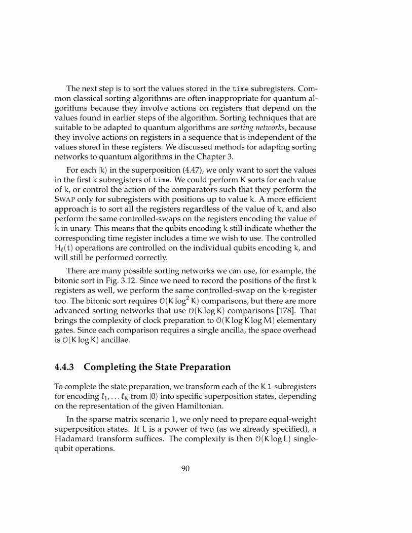
The next step is to sort the values stored in the time subregisters. Com-mon classical sorting algorithms are often inappropriate for quantum al-gorithms because they involve actions on registers that depend on thevalues found in earlier steps of the algorithm. Sorting techniques that aresuitable to be adapted to quantum algorithms are sorting networks, becausethey involve actions on registers in a sequence that is independent of thevalues stored in these registers. We discussed methods for adapting sortingnetworks to quantum algorithms in the Chapter 3.
For each |k〉 in the superposition (4.47), we only want to sort the valuesin the first k subregisters of time. We could perform K sorts for each valueof k, or control the action of the comparators such that they perform theSWAP only for subregisters with positions up to value k. A more efficientapproach is to sort all the registers regardless of the value of k, and alsoperform the same controlled-swaps on the registers encoding the value ofk in unary. This means that the qubits encoding k still indicate whether thecorresponding time register includes a time we wish to use. The controlledH`(t) operations are controlled on the individual qubits encoding k, andwill still be performed correctly.
There are many possible sorting networks we can use, for example, thebitonic sort in Fig. 3.12. Since we need to record the positions of the first kregisters as well, we perform the same controlled-swap on the k-registertoo. The bitonic sort requires O(K log2 K) comparisons, but there are moreadvanced sorting networks that use O(K logK) comparisons [178]. Thatbrings the complexity of clock preparation to O(K logK logM) elementarygates. Since each comparison requires a single ancilla, the space overheadis O(K logK) ancillae.
4.4.3 Completing the State Preparation
To complete the state preparation, we transform each of the K l-subregistersfor encoding `1, . . . `K from |0〉 into specific superposition states, dependingon the representation of the given Hamiltonian.
In the sparse matrix scenario 1, we only need to prepare equal-weightsuperposition states. If L is a power of two (as we already specified), aHadamard transform suffices. The complexity is then O(K logL) single-qubit operations.
90

In scenario 2, the target superposition states for the l-subregisters to beencoding `1, . . . `K are given by (4.37). We propose preparing the requiredtarget superposition states using a similar approach as in Ref. [116], namelyby transducing the computed values α`(t)/αmax (using the output of oracleOcoeff) into quantum amplitudes
√α`(t)/αmax via ‘inequality testing’. Ac-
cording to that approach, the state preparation requires the use of severalregisters. For each k = 1, . . . ,K, in addition to the lk subregister for en-coding the index value `k to identify the coefficients in the decomposition(4.16) and the timek subregister for encoding a particular time tk as partof the |clock〉 state, we introduce two further registers named ‘coeffk’ and‘refk’, each consisting of ν qubits. Here, ν is the number of bits used for theν-bit fixed-point approximations α[ν]
` (t) := b2να`(t)/αmaxc. Finally, an ad-ditional single-qubit ancilla called ‘flag’ is required to distinguish betweenthe two index ranges ` = 0, . . . ,L− 1 and ` = L, . . . , 2L− 1, and thus indicate
which of the corresponding two alternative amplitudes(αmax+α`(t)
2
)1/2and
(αmax−α`(t)
2
)1/2has been generated.
The state preparation by inequality testing can be outlined as follows.For more details, see Ref. [116]. We first create uniform superpositionsin both the lk and the refk register. We then compute a ν-bit fixed-pointapproximation α[ν]
` (t) of the modified coefficient α`(t)/αmax at time t speci-fied by the timek subregister. We obtain the value α[ν]
` (t) by querying theoracle Ocoeff defined in Eq. (4.15) and save it in register coeffk. These firsttwo steps can be formalized by the following state transformations:
|0〉lk |t〉timek |0〉coeffk |0〉refk |0〉flagkH⊗(ν+logL)|·〉lk |·〉refk−−−−−−−−−−−−−→ 1√
L√
2ν
L−1∑`=0
2ν−1∑x=0
|`〉lk |t〉timek |0〉coeffk |x〉refk |0〉flagk
Ocoeff |·〉lk |·〉timek |·〉coeffk−−−−−−−−−−−−−−−−→ 1√L√
2ν
L−1∑`=0
2ν−1∑x=0
|`〉lk |t〉timek∣∣∣α[ν]` (t)
⟩coeffk
|x〉refk |0〉flagk .
(4.48)
Creating the uniform superpositions in the first step requires only ν+ logLelementary gates. Computing α[ν]
` (t) requires only one query to oracle
91
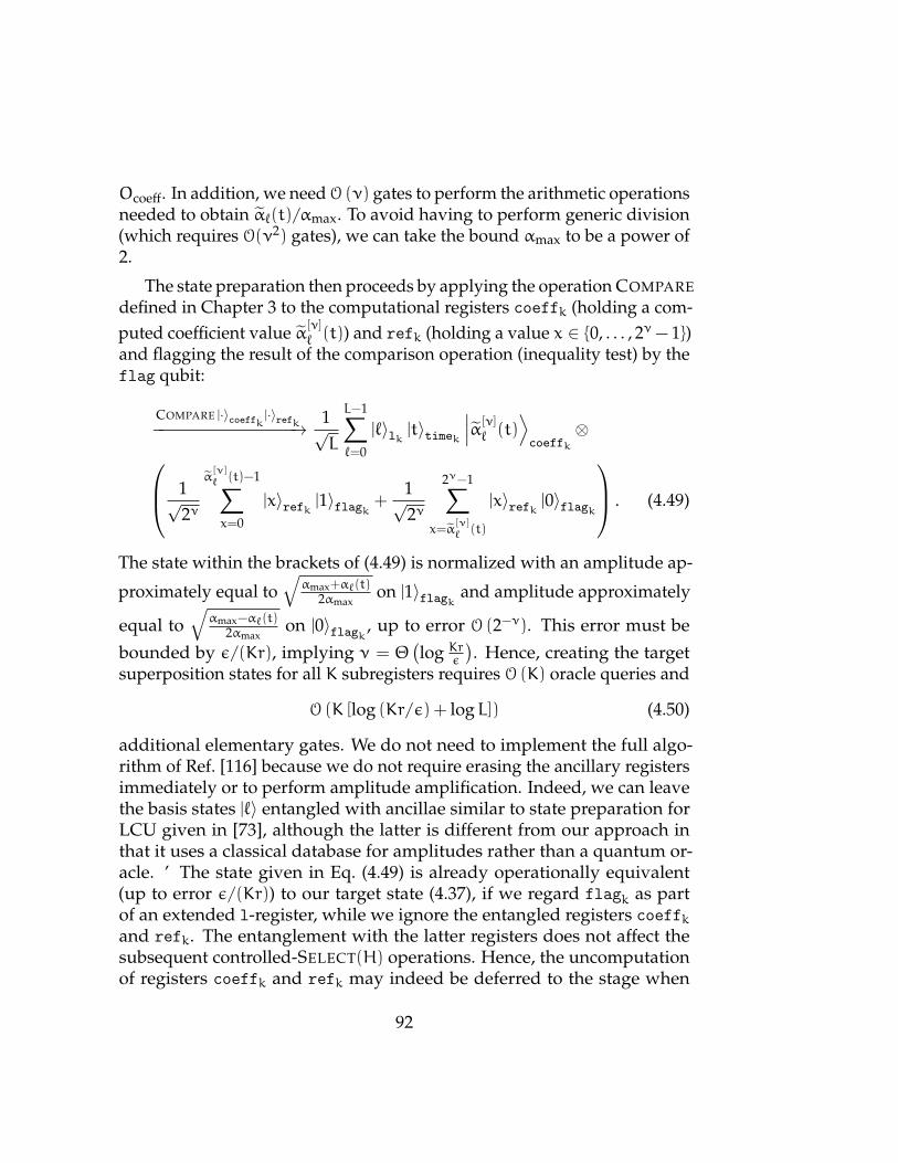
Ocoeff. In addition, we need O (ν) gates to perform the arithmetic operationsneeded to obtain α`(t)/αmax. To avoid having to perform generic division(which requires O(ν2) gates), we can take the bound αmax to be a power of2.
The state preparation then proceeds by applying the operation COMPAREdefined in Chapter 3 to the computational registers coeffk (holding a com-puted coefficient value α[ν]
` (t)) and refk (holding a value x ∈ 0, . . . , 2ν− 1)and flagging the result of the comparison operation (inequality test) by theflag qubit:
COMPARE |·〉coeffk |·〉refk−−−−−−−−−−−−−−−→ 1√L
L−1∑`=0
|`〉lk |t〉timek∣∣∣α[ν]` (t)
⟩coeffk
⊗ 1√
2ν
α[ν]` (t)−1∑x=0
|x〉refk |1〉flagk +1√2ν
2ν−1∑x=α
[ν]` (t)
|x〉refk |0〉flagk
. (4.49)
The state within the brackets of (4.49) is normalized with an amplitude ap-
proximately equal to√αmax+α`(t)
2αmaxon |1〉flagk and amplitude approximately
equal to√αmax−α`(t)
2αmaxon |0〉flagk , up to error O (2−ν). This error must be
bounded by ε/(Kr), implying ν = Θ(log Kr
ε
). Hence, creating the target
superposition states for all K subregisters requires O (K) oracle queries and
O (K [log (Kr/ε) + logL]) (4.50)
additional elementary gates. We do not need to implement the full algo-rithm of Ref. [116] because we do not require erasing the ancillary registersimmediately or to perform amplitude amplification. Indeed, we can leavethe basis states |`〉 entangled with ancillae similar to state preparation forLCU given in [73], although the latter is different from our approach inthat it uses a classical database for amplitudes rather than a quantum or-acle. ’ The state given in Eq. (4.49) is already operationally equivalent(up to error ε/(Kr)) to our target state (4.37), if we regard flagk as partof an extended l-register, while we ignore the entangled registers coeffkand refk. The entanglement with the latter registers does not affect thesubsequent controlled-SELECT(H) operations. Hence, the uncomputationof registers coeffk and refk may indeed be deferred to the stage when
92
reversing the above state preparation as part of B† after completing theSELECT(V) operation.
Next, let us consider the states prepared as a result of these procedures.In the first case, where we prepare the superposition of times by the com-pressed rotations, we first prepare the state |φq〉⊗K+1, which contains theseparations between successive times, then add these to obtain the times.The state is therefore
√1 − µ2
S
K∑k=0
ζk/2 |k〉∑
j1<j2...<jk
|j1, . . . , jk〉+ µ∣∣ν ′′⟩
. (4.51)
The preparation of the registers encoding `1, . . . `K gives a factor of 1/LK/2
for both considered Hamiltonian models. For k < K, the registers past kare not used, and the effective amplitude factor is thus 1/Lk/2. We obtainthe indices j1 to jk in sorted order without repetitions. This means thatthe weightings of the terms in the sum are (γT/(rM))k/2 for scenario 1 and(αmaxT/(rM))k/2 for scenario 2. In Eq. (4.25), when there are no repetitionsthe k1, . . . ,kσ are all 1. Therefore we have approximately the desired statepreparation from Eq. (4.31) with the correct weightings, and with s =S/(1 − µ2). There is imprecision of O(ε/r) due to the additional termweighted by µ, as well as imprecision due to the omitted repetitions, whichare bounded in Section 4.5 below.
For amplitude amplification to take one step, we require
s = S/(1 − µ2) 6 2. (4.52)
Note that it can be less than 2, and oblivious amplitude amplification canstill be performed in a single step using an ancilla qubit, as noted in theSegment Lemma of Ref. [135]. To bound the value of S,
S =∑|x|6K
ζ|x|
=
K∑k=0
(M
k
)ζk
<
∞∑k=0
Mkζk
k!
= eMζ = eλT/r. (4.53)
93
Therefore, by choosing r > λT/ ln[2(1 − µ2)] we can ensure that s 6 2, anda single step of amplitude amplification is sufficient. The value of µ2 isO(ε/r), and therefore r = Θ(λT).
In the second case, where we obtain the superposition over the timesvia a sort, the state is as in Eq. (4.47) except sorted, with information aboutthe permutation used for the sort in an ancilla. When there are repeatedindices j, the number of initial sets of indices that yield the same sortedset of indices is k!/(k1!k2! . . . kσ!), using the same notation as in Eq. (4.25).That means for each sorted set of j there is a superposition over this manystates in the ancilla with equal amplitude, resulting in a multiplying factorof√k!/(k1!k2! . . . kσ!) for each sorted set of j.
As noted above, because the times tk+1 to tK are ignored, the factors ofM in the amplitude cancel. Similarly, when we prepare the state for theregisters encoding `1, . . . `K, we obtain a factor of 1/Lk/2. Including thesefactors, and the factor for the superposition of states in the ancilla, we ob-tain amplitude (γT/(rM))k/2/
√k1!k2! . . .kσ! for scenario 1 and amplitude
(αmaxT/(rM))k/2/√k1!k2! . . . kσ! for scenario 2. Hence we have the desired
state preparation from Eq. (4.31) with the correct amplitudes, and the sames.
We require s 6 2 for oblivious amplitude amplification to take one step.We can bound s via
s =
K∑k=0
Mkζk
k!
<
∞∑k=0
Mkζk
k!
= eMζ = eλT/r. (4.54)
Therefore, by choosing r > λT/ ln 2 we can ensure that s 6 2, and a singlestep of amplitude amplification is sufficient. Note that it is convenientto take r to be a power of two, so the qubits encoding the time may beseparated into a set encoding the segment number and another set encodingthe time within the segment. Hence, in either case we choose r = Θ(λT).
94

4.5 Complexity Requirements
We now summarize the resource requirements of all the components ofthe algorithm and provide the overall complexity. We start with elementsthat are necessary for both scenario 1 sparse matrices and quantum type 2Hamiltonians and then discuss the complexities of their unique parts.
The full quantum circuit consists of r successively executed blocks, onefor each of the r time segments. Since we took r = Θ(λT) for obliviousamplitude amplification, the overall complexity is multiplied by a factor ofλT .
Each segment requires one round of oblivious amplitude amplification,which includes two reflections R, two applications ofW and one applicationof the inverse W†, as in Eq. (4.36). The cost of reflections is negligiblecompared to that ofW. Hence, the overall cost of the algorithm amounts toO(r) times the cost of transformationW, whose quantum circuit is depictedin Fig. 4.2. For scenario 1, implementing W requires the procedure toprepare the |clock〉 state and its inverse, 2K applications of H⊗ logL and Kcontrolled applications of unitaries H`(t). For scenario 2, implementingW requires likewise preparing the |clock〉 state and the reverse of thatprocedure, 2K applications of the controlled-PREP(α) subroutine, and Kcontrolled applications of unitaries H`.
Choosing K as in Eq. (4.24) yields error due to truncation for eachsegment scaling as O(ε/r), and therefore total error due to truncationscaling as O(ε). Taking r = Θ(λT), K is chosen as
K = Θ
(log(λT/ε)
log log(λT/ε)
). (4.55)
Note that λ > Hmax implies that the condition r > HmaxT is satisfied, whichwas required for deriving Eq. (4.24). Recall that λ = Lγ in scenario 1 andλ = Lαmax in scenario 2.
In the case where the |clock〉 state is prepared using the compressedform of rotations, the operation that is applied is a little different thandesired, because all repeated times are omitted. For each k, the proportionof cases with repeated times is an example of the birthday problem and isapproximately k(k− 1)/(2M). Therefore, denoting by Uunique the operation
95

corresponding to U but with repeated times omitted, we have
‖U− Uunique‖ .K∑k=2
(T/r)k
k!k(k− 1)
2MHkmaxspec
=
K∑k=0
(T/r)k+2
k!1
2MHk+2
maxspec
<T2H2
maxspec
2r2MeTHmaxspec/(rM), (4.56)
where Hmaxspec := maxt ‖H(t)‖. The error over r segments due to omittingrepeated times is upper bounded by
r‖U− Uunique‖ .T2H2
maxspec
2rMeTHmaxspec/(rM) . (4.57)
Using r ∈ Θ(λT) and λ > Hmaxspec, we should then choose
M = Ω
(TH2
maxspec
ελ
). (4.58)
Therefore, when the repeated times are omitted, we would take
M = Θ
(T
ελ(H2
maxspec + Hmax)
). (4.59)
Next we consider the gate complexity for the |clock〉k⊗time state prepa-ration. In the case of the compressed rotation encoding, the complexity isO (K logM), where we have used r ∈ Θ(λT). In the case where |clock〉k⊗timeis prepared with a quantum sort, the complexity is O (K logM logK).
4.5.1 Complexity for Scenario 1
Let us now consider the complexity of simulation of a Hamiltonian givenas a sparse matrix. The preparation of the registers `1, . . . , `k requires onlycreating an equal superposition. As we discussed in Section 4.4.3, theHadamard transform in this stage requires O (K logL) elementary gates.
96

Next, one needs to implement the controlled unitaries H`. Each con-trolledH` can be implemented with O (1) queries to the oracles that give thematrix entries of the Hamiltonian [135]. Since the unitaries are controlled byO (logL) qubits and act on n qubits, each control-H` requires O (logL+n)gates. Scaling withM does not appear here, because the qubits encodingthe times only serve as input to the oracles. As there are K controlled oper-ations in each segment, the complexity of this step for a segment is O (K)oracle queries and O (K(logL+n)) additional gates.
As the total cost for the entire simulation is obtained by multiplying thecost per segment by the number r of all segments, the overall oracle querycomplexity thus amounts to
O(λTK) . (4.60)
Here λ = Lγ and L is chosen as in Eq. (4.10) as Θ(d2Hmax/γ), so λ ∈O(d2Hmax). In addition, K is given by Eq. (4.55), giving the total querycomplexity
O
(d2HmaxT
log(dHmaxT/ε)
log log(dHmaxT/ε)
). (4.61)
The overall complexity in terms of the additional gates is larger, anddepends on the scheme used to prepare the state |clock〉k⊗time. In thecase where the preparation is performed via the compressed encoding, weobtain the complexity
O (λTK[logL+ logM+n]) . (4.62)
Regardless of the preparation approach, γ is chosen as in Eq. (4.9) asΘ(ε/(d3T)). Moreover, L ∈ Θ(d5HmaxT/ε), whereas the first term in thescaling forM in Eq. (4.59) is O(d2HmaxT/ε). This means that the first termin Eq. (4.59) can be ignored in the overall scaling due to the logL, and weobtain an overall scaling of the gate complexity as
O
(d2HmaxT
log(dHmaxT/ε)
log log(dHmaxT/ε)
[log(dHmaxT
ε
)+ log
(HmaxT
εdHmax
)+n
]).
(4.63)There is also complexity of O(r log r) for the increments of the registerrecording the segment number, but it is easily seen that this complexity isno larger than the other terms above.
97

In the case where |clock〉k⊗time is prepared using a sorting network, weobtain complexity
O (λTK(logL+ logM logK+n)) , (4.64)
withM given by Eq. (4.24).
Technically, this complexity is larger than that in Eq. (4.63), because ofthe multiplication by logK. Nevertheless, preparation by a sorting networkmay turn out to sometimes be advantageous in practice because the firstpreparation requires a larger value ofM. This is because the compressedencoding approach does not contain repeated times whereas the approachby sorting networks does.
4.5.2 Complexity for Scenario 2
Let us now consider the cost of simulating the time evolution generated byscenario 2 Hamiltonians. For each single time segment, we have 3× (2K)applications of the controlled-PREP(α) operation as part of B and B† whenimplementing W (or W†), which in turn must be applied three times forachieving oblivious amplitude amplification. This requires O (K) queries toOcoeff. Furthermore, we have 3K controlled-SELECT(H) operations as partof the SELECT(V) transformation that is involved three times in obliviousamplitude amplification, which thus require O (K) queries to Ounit. Notethat the mentioned query complexities for Ocoeff and Ounit are additive.Hence, the overall query complexity for the entire simulation over all r timesegments amounts to O (rK), which, by using r ∈ Θ(λT) and λ = Lαmax aswell as the choice for K given in Eq. (4.55), becomes
O
(LαmaxT
log(LαmaxT/ε)
log log(LαmaxT/ε)
). (4.65)
For each time segment, preparation of the auxiliary l-register statesrequires O (K(logL+ log (rK/ε)) additional elementary gates, as displayedearlier in Eq. (4.50). Furthermore, we need O(K) gates to implement the mi-nus signs given in Eq. (4.18) as well as the the (−i)k factors occurring in theDyson series. Additional gate complexity comes from the preparation of the
98

|clock〉k⊗time state, which is the same as for scenario 1. Preparation via com-pressed encoding thus requires in total O
(λTK
[logL+ logM+ log
(λTKε
)])
gates, where we have repeatedly used r ∈ Θ(λT). Using once moreλ = Lαmax and Eqs. (4.55) and (4.59) together with Hmax 6 Lαmax, thisfinally yields
O
(αmaxLT
log (αmaxLT/ε)
log log (αmaxLT/ε)
[log(αmaxLT
ε
)+ log
(HmaxT
εαmaxL
)
+ log(
log (αmaxLT/ε)
log log (αmaxLT/ε)
)+ logL
])(4.66)
as the overall gate complexity in this case, where we again ignored the firstterm in Eq. (4.59) in the overall scaling due to the occurrence of the largerlog (αmaxLT/ε) term. Observe that the last two additive terms logK andlogL in the brackets of Eq. (4.66) are also much smaller compared to the firstterm; they have also been ignored in the formulation of Theorem 2. Simi-larly, we obtain the gate complexity O
(λTK[logL+ logM logK+ log
(λTKε
)])
for implementations based on quantum sorting networks, which is slightlylarger due to the additional logK factor in the second term.
Scaling with n (i.e. with the number of system qubits) does not appearin Eqs. (4.65) and (4.66), because the system qubits are just used as inputto the oracle Ounit (defined in Eq. (4.14)) as part of controlled-SELECT(H)operations. The scaling with n is therefore hidden in the gate cost ofimplementing that oracle.
4.6 Results
Let us summarize the results by stating the theorems for both scenarios.
Theorem 6 (Time-dependent Hamiltonian simulation for sparse matrices)For a Hamiltonian H(t) given by a time-dependent d-sparse matrix, the generatedtime evolution of a quantum system can be simulated for time T and within errorε using a number of oracle queries scaling as
O
(d2HmaxT
log(dHmaxT/ε)
log log(dHmaxT/ε)
), (4.67)
99

and a number of additional elementary gates scaling as
O
(d2HmaxT
log(dHmaxT/ε)
log log(dHmaxT/ε)
[log(dHmaxT
ε
)+ log
(HmaxT
εdHmax
)+n
]).
(4.68)
Theorem 7 (Time-dependent Hamiltonian simulation for LCU)For a HamiltonianH(t) given by a time-dependent linear combination of L unitaryterms, the generated time evolution of a quantum system can be simulated for timeT and within error ε using a number of oracle queries scaling as
O
(LαmaxT
log(LαmaxT/ε)
log log(LαmaxT/ε)
)(4.69)
and a number of additional elementary gates scaling as
O
(LαmaxT
log (LαmaxT/ε)
log log (LαmaxT/ε)
[log(LαmaxT
ε
)+ log
(HmaxT
εLαmax
)]),
(4.70)where αmax denotes a known global upper bound on the modulus of each of the Ltime-dependent coefficients in the decomposition, implying Lαmax > Hmax.
4.7 Applications
Our algorithm can be used for a range of problems that require simulatingdynamics under a time-dependent Hamiltonian. We now outline severalspecific applications.
Low and Wiebe recently proposed a new Hamiltonian simulation al-gorithm in the interaction picture [37]. This algorithm uses simulationof a time-dependent Hamiltonian as a subroutine. Taking a HamiltonianH = A+ B and the Schrodinger equation i∂t |ψ(t)〉 = (A+ B) |ψ(t)〉, wecan formulate the simulation problem in the interaction picture as
HI(t) = eiAtBe−iAt, (4.71)
|ψI(t)〉 = eiAt |ψ(t)〉 , (4.72)
i∂t |ψI(t)〉 = eiAtBe−iAt |ψI(t)〉 , (4.73)
100

where HI is the interaction picture Hamiltonian, |ψI(t)〉 a state in the in-teraction picture and (4.73) the interaction picture Schrodinger equation.Solving (4.73) requires time-dependent Hamiltonian simulation. Low andWiebe [37] proposed an approach for simulating time-dependent Hamilto-nians simultaneously with us. They use a simpler method of preparing thestate representing the times by discarding times rather than sorting them.This simplification results in a multiplicative factor in the gate complexity.
Interaction picture simulation is useful when ‖A‖ ‖B‖ and e−iAt isstraightforward to implement. Using the interaction picture then allowsus to reduce the complexity in terms of the norm of the Hamiltonian. Thisapproach is particularly useful for quantum chemistry where it allows fora simulation with complexity sublinear in the number of orbitals [74].
The second application of time-dependent simulations is adiabatic com-puting and quantum annealing. Adiabatic computation is performed bypreparing the ground state |ψ〉 of an “easy” Hamiltonian H0 and thenevolved under a slowly changing Hamiltonian
H(t) = tH1 + (1 − t)H0, (4.74)
where H1 is the Hamiltonian whose ground state we wish to prepare [186].If the evolution is slow enough to satisfy the conditions of the adiabatictheorem [187], one has a a good chance of preparing the ground state ofH1. These approaches are favored for heuristics for optimization problems.Implementing them on a fault-tolerant circuit-based quantum computercan allow for a higher accuracy than using an analog quantum annealer.This implementation would simply consist of simulating the evolutionunder a time-dependent Hamiltonian.
Our work can also be applied to state preparation. Adiabatic statepreparation is a popular choice for initializing quantum chemistry algo-rithms [71]. In this case, one prepares an eigenstate of a simple Hamiltonianand slowly (adiabatically) changes the Hamiltonian to the one of interest.
Lastly, there are many time-dependent phenomena that our algorithmcan simulate. One example is evolution of states under a time-dependentelectromagnetic field. In quantum chemistry and material science, we canaccount for nuclear movement by describing the system of electrons by atime-dependent Hamiltonian.
101

4.8 Conclusion
We have provided a quantum algorithm for simulating the evolution gen-erated by a time-dependent Hamiltonian that is either given by a genericd-sparse matrix or by a time-dependent linear combination of some effi-ciently implementable unitary terms. For both scenarios, the complexity ofthe algorithm scales logarithmically in both the dimension of the Hilbertspace and the inverse of the error of approximation ε. Our work presentsan exponential improvement in error scaling compared to techniques basedon Lie-Trotter-Suzuki expansion. We utilize the truncated Dyson series,which is based on the truncated Taylor series approach by Berry et al. [34].It achieves similar complexity, in that it has T times a term logarithmic in1/ε. Interestingly, the complexity in terms of queries to the Hamiltonian isindependent of the rate of change of the Hamiltonian.
For the complexity in terms of additional gates, the complexity is some-what larger and depends logarithmically on the rate of change of the Hamil-tonian. The complexity also depends on the scheme that is used to preparethe state to represent the times. If one uses the scheme as in Ref. [136],which corresponds to a compressed form of a tensor product of small ro-tations, then there is an additional error due to the omission of repeatedtimes. Alternatively, one could prepare a superposition of all times and sortthem, which eliminates that error, but gives a multiplicative factor in thecomplexity. This trade-off means that different approaches may be moreefficient with different combinations of parameters.
Simultaneously with the publication of our algorithm, Low and Wiebe [37]developed a similar algorithm for time dependent Hamiltonians also basedon LCU. Their algorithm is slower than ours by a multiplicative factor.Even more recently, Berry et al. [188] came up with a new algorithm thatimproved the dependence on the norm of the Hamiltonian. Their workbuilds onto [149] and can provide more efficient algorithm for simulationHamiltonians whose norm significantly changes over time, for example inscattering problems.
An interesting open question is whether the complexity could be im-proved such that the factor of log(1/ε) is additive rather than multiplica-tive, as in Ref. [35] for time-independent Hamiltonians. However, thoseapproaches do not appear directly applicable to the time-dependent case.
102

5Training and Tomography withQuantum Boltzmann Machines
“What I cannot create, I do not understand.”
Richard Feynman
Machine learning (ML) has earned a prominent role in the tech industryfor its ability to train computers for complicated tasks without the need ofgiving them explicit instructions. ML performs exceptionally well on taskswith complex structure such as speech recognition [189–191], computervision [192–194] or even playing the board game Go [195–197]. Given itsimportance for computing, it is natural to ask what can arise from theconfluence of ML and quantum computing.
In this chapter, we focus on quantum algorithms that learn from quan-tum data. This chapter is based on our paper [4] and significantly over-laps with it. I altered the text to suit an audience mostly unfamiliar withBoltzmann machines. I included the Theorems 9 and 10 proved by myco-authors but without the full statements of the proofs. My co-author also
103

carried out the numerical analysis for tomography using relative entropyin Section 5.6.5.
It should be noted that the success of a particular ML algorithm isseldom determined by theoretical analysis alone. Instead, ML algorithmsare compared by running against each other on benchmark sets or by theirusefulness for practical tasks. Since we do not have quantum hardwarethat can run QML algorithms, our situation is similar to the one of artificialintelligence in the 60s. At the same time, the foundations of AI laid backbefore ML became “practical” were crucial for guiding our thinking aboutalgorithm development. Similarly, there is value in foundations research inQML.
5.1 Quantum Machine Learning
ML and quantum physics can overlap in several ways. There are manyresults that apply (classical) ML techniques on quantum problems incondensed-matter physics [198], quantum control [199] or discoveringphysical concepts [200]. In these applications, ML is used to uncover theproperties of physical systems or devise models for complex phenomena.
Another avenue of research explores the implementation of ML algo-rithms on quantum hardware. A number of results showed that quantumcomputing can provide significant speedups for problems such as sup-port vector machines (SVM) [201], nearest neighbor classification [202, 203],boosting [204, 205] and many others [206–210]. However, loading and ac-cessing large data sets in a quantum computer is problematic [211–213].Nevertheless, there are still applications with polynomial speedup andunexplored ways of combining ML with quantum computing techniques.
The last possible way of combining quantum computing and ML isinventing quantum machine learning (QML) algorithms that run on aquantum computer and are designed to process quantum data. In this setup,quantum states are fed into a quantum computer for analysis directly froman experiment or another quantum device. This area has a lot of potentialfor speedups. To analyze the data classically, one needs to first performtomography whose complexity scales exponentially with the size of thesystem. Quantum machine learning on quantum data might allow us
104

to extract features from the system without performing full tomography.While we do not expect universal exponential speedups in this area, it islikely that using quantum machine learning will assist in quantum systemcharacterization and Hamiltonian learning [214, 215] for problems thatexhibit some structure. We summarize the types of quantum machinelearning in the table below.
The data isclassical quantum
Thealgorithmruns on a
classicalcomputer Classical ML
ML onexperimental
dataquantumcomputer
QML for SVM,clustering, fitting . . . This chapter
Figure 5.1: Different areas of QML. Our focus is on quantum algorithmsable to process quantum data. However, since classical data are a specialcase of quantum ones, we show how to learn on them as well.
5.2 Boltzmann Machines
As the name of this chapter implies, we are interested in a particular neuralnetwork called a Boltzmann machine (BM). The Boltzmann machine isa physically motivated framework capable of generating new examples“similar” to the training data [216], i.e. generative, unsupervised trainingintroduced in Appendix A1. The inspiration for Boltzmann machinescomes from statistical physics, particularly the Boltzmann distribution.For readers unfamiliar with machine learning we recommend readingAppendix A first and then continuing with this section.
Hinton [217] defines a Boltzmann machine as “a network of symmet-rically connected, neuronlike units that make stochastic decisions aboutwhether to be on or of.” This network has two key features – a graph (or ahypergraph1) and an energy function. Just as for general neural networks,
1A hypergraph is a generalization of a graph. While an edge in a graph connects twovertices, a hyperedge in a hypergraph can connect any number of vertices.
105

the information vector x is encoded in the vertices (called units) xi that cantake on values ±1. The units of a BM consist of visible units and optionalhidden units, similarly to other artificial neural networks.
The edges of the graph have been assigned weights such that an edgeconnecting nodes i and j has weightWij. Missing edges automatically haveweight 0. We also allow for self-loop like terms, biases bi. This energyfunction
E(x) = xTWx + bTx (5.1)
can be shown to be equivalent to (A.1) where we added one bit to x with afixed value of 1. We demonstrate how to compute an energy for a givenconfiguration in Fig. 5.2.
3 -2
5-2 3
-1
1 -1
1
Figure 5.2: Each configuration can be assigned an energy value. In thisexample, the assigned configuration E = (−1)·1 + (−2)·1 + 3·(−1) + 3· 1·1 + (−2)·1·(−1) + 5·1·(−1) = −6.
Common choices of the graph include the complete graph and thebipartite graph (see Fig. 5.2) with connections only between visible andhidden units. A BM defined on a bipartite graph is called a RestrictedBoltzmann Machine (RMB). RBMs are favored by the ML communitybecause they can be trained using an efficient method called contrastivedivergence [218].
A properly trained BM generates new data. Outputs similar to thetraining set should be generated with high probability while data that isvery different than the training set should be very unlikely to appear. Todo this, we assume that there is a distribution P(v) that the model learnsand the training data are sampled from it. A BM accomplishes this byoutputting data from its probability distribution Q(v), defined by weightsand biases, that should be close to the distribution P(v). We accomplish
106

(a) A fully-connected Boltzmannmachine. The connections be-tween units form a completegraph.
(b) Restricted Boltzmann Ma-chine. Each hidden unit is con-nected to each visible unit butnot to other hidden units andvice versa. The connections forma bipartite graph.
Figure 5.3: Fully connected vs. restricted Boltzmann machine.
this by teaching the BM to approximately reproduce the training data2. Inparticular, the probabilityQ(x) for a configuration x (i.e. on both the visibleand the hidden units) is defined as:
Q(x) =exp (−E(x))∑x exp (−E(x))
. (5.2)
This is the Boltzmann distribution for the energy E(x) defined in (5.1) wherewe set kT = 1. The state x consists of the state on the hidden units h andvisible units v, so x = (v, h). The probability of a state on the visible unitscan be obtained by summing over all configurations on the hidden units
Q(v) =∑
h exp (−E(v, h))∑v,h exp (−E(v, h))
. (5.3)
But how do we get the weights and biases required for computing (5.1)and (5.3)? We train the algorithm to make Q close to P using the train-ing data. The “closeness” of two distributions is measured by Kullback-Leibler (KL) divergence. Formally, the KL divergence quantifies the in-formation loss occurring if the distribution generated from the model Q
2We want to be able to model the training data but not overfit them.
107
replaces the underlying distribution of data P:
DKL(P‖Q) =∑
vP(v) log
P(v)Q(v)
. (5.4)
Since P is fixed, minimizing DKL(P‖Q) is equivalent to maximizing thelog-likelihood
L =∑
vP(v) logQ(v). (5.5)
While computing DKL(P‖Q) (and the log-likelihood) is exponentially dif-ficult in the number of units, it is possible to estimate its gradients withrespect to bi andWi,j. A straightforward computation yields
∂biL =∑
vP(v)
[−
∑h xi exp (−E(v, h))∑
h exp (−E(v, h))+
∑v ′,h xi exp (−E(v ′, h))∑
v ′,h exp (−E(v ′, h))
]
(5.6)for biases and
∂Wi,jL=∑
vP(v)
[−
∑h xixj exp (−E(v, h))∑
h exp (−E(v, h))+
∑v ′,h xi exp (−E(v ′, h))∑
v ′,h exp (−E(v ′, h))
]
(5.7)for weights. However, we do not have direct access to the probabilitydistribution P(v). Instead, we estimate the gradients as
∂Wi,jL =1s
∑v∈training set
[−
∑h xixj exp (−E(v, h))∑
h exp (−E(v, h))+
∑v ′,h xi exp (−E(v ′, h))∑
v ′,h exp (−E(v ′, h))
]
(5.8)
where s is the number of training vectors. Here we approximated theunderlying distribution P(v) using the training data which we treat assamples from P(v). We estimate the gradients of the biases in the sameway. The expression (5.8) consists of expectations values of xixj in twodifferent types of states. The first term in (5.8) is the expectation valuewhen the visible units are “clamped” to a particular training vector v (i.e.fixed to a given configuration) while the hidden units model a thermaldistribution. We first estimate these expectation values through samplingfor each training vector, and then we average them over the data set. The
108

second term in (5.8) does not depend on the training data, thus we need to
compute it only once for each update of weights. The term∑
v,h xi exp (−E(v,h))∑v,h exp (−E(v,h))
is sampled from a thermal distribution on all units. The steps of the trainingare summarized at the end of this section.
Hinton and Sejnowski [219] proposed the first machine learning al-gorithm that evaluates the gradient in Eq. (5.8). However, this learningwas not efficient because it required many samples from a thermal dis-tribution. There have been many approaches to improve the speed oflearning [220, 221, 221–223]. Most notably, the first term in (5.8) can be com-puted exactly for RBMs and the second term can be roughly approximatedusing a method called contrastive divergence. Surprisingly, this very roughapproximation works exceptionally well [217, 218, 224].
We train a BM using stochastic gradient ascent. We start by initializ-ing the weights and biases to random values and keep updating them toincrease L (and therefore decrease DKL(P‖Q)). Many techniques can beused to speed up the convergence of gradient descent, including changingthe gradient step and including momentum3. This process is repeated fora fixed number of epochs. If the number of epochs is too small, P andQ might not be close. On the other hand, if we trained for too long, it ispossible that the BM overfits the data. Since L is impossible to estimate forreal-world data sets, the quality of the model is in practice estimated usingcross-validation data.
We will conclude this section with an overview of the training and thegenerating algorithms. Once we settle on a graph (i.e., the number of visibleand the hidden units and the connections between them) for the BM, thealgorithm proceeds as follows:
3Momentum often helps accelerate gradient descent. The name is inspired by mechan-ics and suggests that instead of following the direction of the gradient (acceleration), weshould follow the direction of velocity. In each step, the new momentum pi+1 is calculatedas a linear combination of momentum in the previous step pi and freshly computedgradient ai+1. The new momentum is pi+1 = (1 −α)pi +αai+1 where α ∈ [0, 1].
109

Boltzmann machine training
generate starting weights and biasesconstruct the energy functionfor the number of epochs do
create an approximation of the thermal distribution on all unitsevaluate the expectation values of xixj and xi in this configurationfor all training vectors do
clamp visible units to a training vectorcreate an approximation of the thermal state on hidden unitsevaluate the expectation values xixj and xi in this configuration
end forcompute gradientsupdate weights and biasesupdate the energy function
end for
Once the algorithm is trained, we can generate new data:
Sampling from a Boltzmann machine
create an approximation of the thermal state on all unitssample from the visible units
5.3 Training Quantum Boltzmann Machines
There are two main reasons why it is worth introducing Boltzmann ma-chines to quantum mechanics. First, classical BMs may require many hid-den units to model complicated datasets. We know that quantum mechan-ics can produce distributions that are difficult to sample from classically.It is possible that quantum Boltzmann machines will be more space effi-cient than classical ones. Second, we want to perform generative learningon quantum data. We will now introduce several approaches for quan-tizing BMs and compare them between each other and to their classicalcounterparts.
A quantum Boltzmann machine (QBM) was first introduced by Aminet al. [225]. The QBM was defined as a generalization of a classical Boltz-
110
mann machine to the quantum regime. Classical binary units are replacedby qubits and the energy function by a Hamiltonian. Amin et al. con-strained their Hamiltonians to the transverse Ising model.
This choice was made to satisfy the hardware abilities; this algorithmwas designed to run on a D-Wave machine. While such models are trainableand can outperform classical BMs, the training procedure proposed thereinsuffers two drawbacks. First, the transverse field cannot be learned bygradient descent from classical data. These terms must be found throughbrute force techniques which makes finding the full Hamiltonian muchmore difficult. Second, the transverse Ising models considered are widelybelieved to be efficiently simulatable using quantum Monte-Carlo methodsand therefore do not provide a clear quantum advantage. The state of theQBM can be then described by the density matrix corresponding to thethermal state of the Hamiltonian
σ =e−H
Tr [e−H](5.9)
and the state on the visible units
σv = Trh [σ] =Trh[e−H
]
Tr [e−H], (5.10)
where we traced over the hidden units. Amin et al. further defined quan-tum log-likelihood for training QBMs on classical states. In this chapter, wegeneralize their version of the QBM in more than one way.
We explicitly design QBMs to process quantum data and work withmodels that exhibit the full power of quantum computing. The gener-alization of Boltzmann Machine training into the quantum setting is notunique. We propose three methods that we refer to as POVM-based Golden-Thompson training4, commutator training, and state-based Relative En-tropy training. These approaches present different quantum analogs of thetraining set and the objective function. We now review the possible realiza-tions of a quantum training set. Next, we follow up with our proposal for anew objective function.
4POVM stands for a positive-operator valued measure. This is the most generalmeasurement.
111

5.3.1 Quantum Training Set
In the classical setting, the training set is a set of vectors representing thedata. As a part of the training of classical Boltzmann Machines (BMs), wehave to ability to fix (clamp) the visible units to a particular training vector.Additionally, we assume that the training set is sampled from an underlyingdistribution P(v) over the visible units. The training set was first translatedto the quantum world as a set of projectors [225] on computational states.This choice makes it indeed possible to clamp visible units on any desiredconfiguration. The goal of the training is then to learn the probability ofeach projector.
We propose two ways of generalizing the training set to include quan-tum as well as classical data. Our first suggestion is that there is no needto constrain ourselves to projectors on computational states. We realizedthat POVMs provide a natural way to express the training set. Formally,we define the training set to be the following.
Let H := HV ⊗HH be a finite-dimensional Hilbert space and let HV
and HL be subsystems corresponding to the visible and hidden units ofthe QBM. The probability distribution pv and POVM Λ = Λv, comprise atraining set for QBM training if
1. there exists a bijection between the domain of pv and Λ and
2. the domain of each Λv is H, and it acts non–trivially only on subsys-tem HV .
Note that unlike P(v), pv corresponds only to the relative frequencies ofeach outcome in the training set and not necessarily to the expectationvalues of each Λv in the underlying state (although we assume that theyshould be close).
This means that if we are training on quantum data, we can take a setof measurements and the frequencies of their corresponding outcomes asour training examples. We can also use POVM training on classical data bypretending that they were sampled from a quantum state.
As a method for generalizing classical data, the choice of POVMs givesa lot of freedom. Let us clarify the freedom of choosing the POVM on
112

an example. Suppose that we wish to train a model that generates evennumbers between 1 and 16 (this was an arbitrary choice) given a set ofsamples that are all even numbers5. Then a sensible training set would be
Λn = |2n〉 〈2n| for 1 6 n 6 8
Λ0 = I −
8∑n=1
Λn, pv = (1 − δv,0)/8. (5.11)
The following equivalent training set can also be used
Λ1 =18(|2〉+ · · ·+ |16〉
)(〈2|+ · · ·+ 〈16|
),
Λ0 = I −Λ1, pv = δv,1. (5.12)
This ambiguity about the form of the training set reveals that the POVM forquantum Boltzmann training can be non-trivial even when a single trainingvector is used. This allows us to circumvent problems with the Golden-Thompson method that arose in [225] by using inherently non-diagonalPOVM elements. POVM training allows for clamping the visible units inthe same way as in the classical case. Just as with classical training data,we assume to have a full knowledge about the data set. We know whichPOVM we measured as well as how often we obtained each outcome6.What we do not know is the underlying quantum state that the outcomeswere sampled from.
The second option is to train directly from quantum states. This isequivalent to a quantum algorithm sampling from a density matrix. Notethat a single density matrix is sufficient since a linear combination of densitymatrices is a density matrix as well. Since learning a description of aquantum state is the goal of tomography, QBM training can be considereda tomographic tool. The training state is then described by a Hamiltoniansuch that the thermal state of this Hamiltonian is close to the training state.
These generalizations give very different notions of what a quantumtraining set really is. While our POVM approach focuses on the general-ization of obtaining (measuring) the training examples, the density matrix
5This is a very simple example where the training set provides all the necessary infor-mation about the concept we are trying to learn without any noise.
6It might be possible to relax this assumption and only assume to have oracular accessto POVM elements.
113
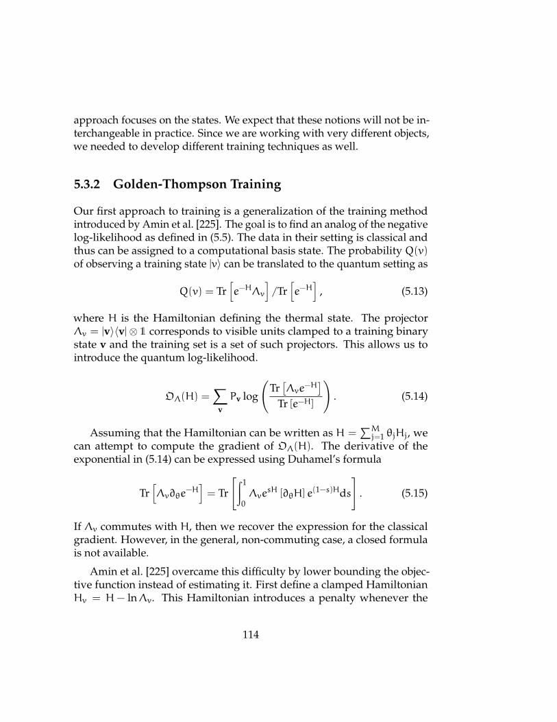
approach focuses on the states. We expect that these notions will not be in-terchangeable in practice. Since we are working with very different objects,we needed to develop different training techniques as well.
5.3.2 Golden-Thompson Training
Our first approach to training is a generalization of the training methodintroduced by Amin et al. [225]. The goal is to find an analog of the negativelog-likelihood as defined in (5.5). The data in their setting is classical andthus can be assigned to a computational basis state. The probability Q(v)of observing a training state |v〉 can be translated to the quantum setting as
Q(v) = Tr[e−HΛv
]/Tr
[e−H
], (5.13)
where H is the Hamiltonian defining the thermal state. The projectorΛv = |v〉〈v|⊗ 1 corresponds to visible units clamped to a training binarystate v and the training set is a set of such projectors. This allows us tointroduce the quantum log-likelihood.
OΛ(H) =∑
vPv log
(Tr[Λve
−H]
Tr [e−H]
). (5.14)
Assuming that the Hamiltonian can be written as H =∑Mj=1 θjHj, we
can attempt to compute the gradient of OΛ(H). The derivative of theexponential in (5.14) can be expressed using Duhamel’s formula
Tr[Λv∂θe
−H]= Tr
[∫1
0Λve
sH [∂θH] e(1−s)Hds
]. (5.15)
If Λv commutes with H, then we recover the expression for the classicalgradient. However, in the general, non-commuting case, a closed formulais not available.
Amin et al. [225] overcame this difficulty by lower bounding the objec-tive function instead of estimating it. First define a clamped HamiltonianHv = H − lnΛv. This Hamiltonian introduces a penalty whenever the
114

visible units are not settled on v. Then, they use the Golden-Thompsoninequality
Tr[eAeB
]> Tr
[eA+B
](5.16)
on expression (5.14), leading to an objective function lower bound
OΛ(H) > OboundΛ (H) =
∑vPv log
(Tr[e−Hv
]
Tr [e−H]
). (5.17)
The components of the gradient of OboundΛ (H) are
∂OboundΛ (H)
∂θj=∑
vPv
(−
Tr[e−Hv∂θjH]Tr[e−Hv ]
+Tr[e−H∂θjH]
Tr[e−H]
). (5.18)
A downside of this approximation is that when Tr[e−Hv∂θjH] = 0, themodel does not learn because the gradient of the Golden-Thompson ap-proximation is zero. However, this does not mean that the gradient of thelog-likelihood is zero as well. Instead, it shows that the upper bound givenby the Golden-Thompson inequality is not always tight. As a consequence,Amin et al. in [225] were not able to use this form of training to learnnon-diagonal terms of the Hamiltonian.
Our work presents two improvements over [225]. First, our formal-ism avoids the problem of Tr[e−Hv∂θjH] = 0 by explicitly designing non-diagonal POVM elements. We can always see a classical distribution asbeing sampled from pure states. This allows us to always pick non-diagonalΛv.
This freedom allows us to choose a POVM that always produces anon-zero gradient because Λv does not commute with H. This avoids theproblems in [225] with the transverse Ising model and a training set similarto (5.11).
Second, our algorithm is not constrained by the transverse Ising model.A general Hamiltonian that is a smooth function of its parameters is indeedpossible. In our numerical analysis, we used an electronic Hamiltonianwhich is 4-local. A choice of a 2-local Hamiltonian is preferred becausesuch a Hamiltonian can be represented on a graph instead of a hypergraph.
115

5.3.3 Commutator Training
Our second approach to POVM training avoids the use of the Golden–Thompson inequality. Instead, we approximate the derivative in the ex-pression (5.14) as a commutator series. If H and Λv commute, we recoverthe classical gradient exactly. In general, if the Hamiltonian is a sum ofbounded Hamiltonian terms the expectation value can be written as acommutator series; we have Tr[Ce−H] for
C := Λv
(∂θjH+
[H,∂θjH]2!
+[H, [H,∂θjH]]
3!+ · · ·
). (5.19)
Thus, the gradient of the average log-likelihood becomes
OΛ(H)
∂θj=∑
vPv
(−
Tr[e−HC]Tr[e−H]
+Tr[e−H∂θjH]
Tr[e−H]
). (5.20)
Next, we truncate the series at a low order. This makes the commutatorseries tractable and we will not incur substantial error if ‖[H,∂θjH]‖ 1. Commutator training is therefore expected to outperform Golden-Thompson training in the presence of L2 regularization on the quantumterms. However, computing higher-order commutators is computationallymore expensive than estimating the gradient from formula (5.18). Lastly,our numerical examples showed that commutator training can be numer-ically unstable. While it might work for certain data sets or be used forfine-tuning a model trained using the Golden-Thompson approach, we didnot find the commutator training to be broadly applicable.
5.3.4 Relative Entropy Training
The relative entropy is the quantum equivalent of KL divergence and assuch, represents a natural extension for the learning of quantum states.Relative entropy is defined as
S(ρ‖σ) = Tr(ρ log ρ− ρ logσ), (5.21)
where ρ is the data distribution and σ = e−βH/Z is the thermal state gener-ated by QBM. For simplicity, we take β = 1. Similarly to KL divergence,
116

the first part of (5.21) is independent of the parameters of the QBM. Hence,our goal is to maximize the new objective function
Oρ(H) = Tr[ρ log
(e−H
Tr[e−H]
)]. (5.22)
Minimization of Oρ(H) allows us to train on quantum data, i.e. copies of ρ.We can express the derivatives of Oρ(H) with respect to the parameters ofthe Hamiltonian θ as
∂Oρ(H)
∂θj= −Tr[ρ∂θjH] + Tr[e−H∂θjH]/Tr[e−H]. (5.23)
We can use the expression (5.23) for gradient ascent. We can computean approximation of the gradient by estimating both terms in (5.23). Thefirst term can be obtained by measuring expectation values on the train-ing state and the corresponding expectation values on the approximationof the thermal state created by a simulation. Furthermore, maximizingOρ(H) guarantees that the generated data is close to the training data be-cause S(ρ||e−H/Z) > ‖ρ− e−H/Z‖2/2 ln(2) if ρ is positive definite. Thus ifS(ρ||e−H/Z)→ 0 then e−H/Z→ ρ.
Training by minimizing the relative entropy has two main advantages.First, unlike Golden-Thompson training, no approximations are needed forcomputing tomography. Second, relative entropy can be used for directlylearning quantum states. Given enough copies of the training state ρ andsufficient computing time, relative entropy training provides a classicaldescription of the training state ρ in the form of the parameters θj of aHamiltonian such that ρ ≈ e−H
Tr[e−H] . This provides a novel approach to partialtomography. Unlike tomography, QBM provides a direct description ofthe state but might be more efficient for high-dimensional states exhibitingclear structure. Additionally, QBM has the ability to create additionalapproximate copies of ρ and therefore perform approximate cloning. Wealso propose using QBM as a candidate for a quantum memory (QRAM).
We compare training and generation of Golden-Thompson and relativeentropy QBMs in the diagram 5.4.
117
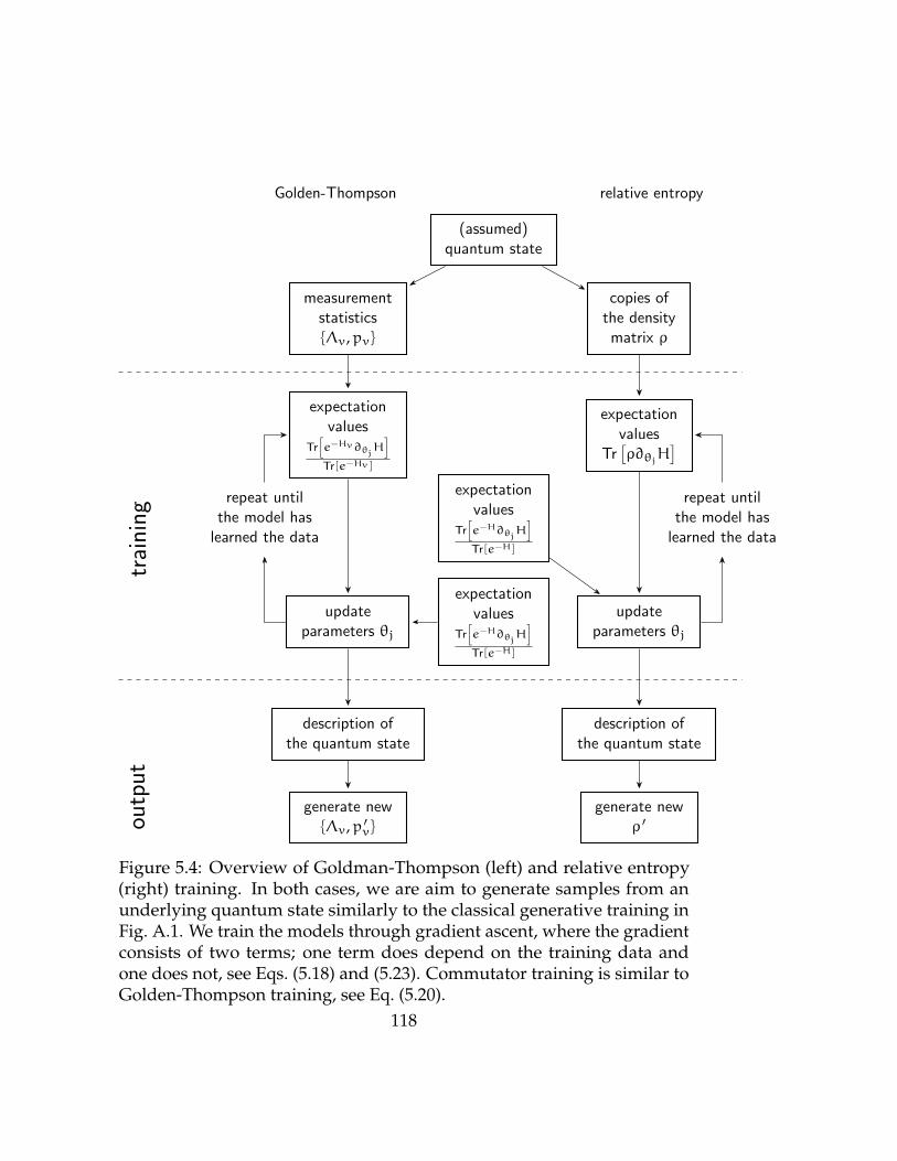
(assumed)quantum state
measurementstatisticsΛv,pv
copies ofthe density
matrix ρ
expectationvalues
Tr[e−Hv∂θjH
]
Tr[e−Hv ]
expectationvalues
Tr[ρ∂θjH
]
expectationvalues
Tr[e−H∂θjH
]
Tr[e−H]
expectationvalues
Tr[e−H∂θjH
]
Tr[e−H]
updateparameters θj
updateparameters θj
repeat untilthe model has
learned the data
repeat untilthe model has
learned the data
description ofthe quantum state
description ofthe quantum state
training
generate newΛv,p ′v
generate newρ ′ou
tput
relative entropyGolden-Thompson
Figure 5.4: Overview of Goldman-Thompson (left) and relative entropy(right) training. In both cases, we are aim to generate samples from anunderlying quantum state similarly to the classical generative training inFig. A.1. We train the models through gradient ascent, where the gradientconsists of two terms; one term does depend on the training data andone does not, see Eqs. (5.18) and (5.23). Commutator training is similar toGolden-Thompson training, see Eq. (5.20).
118

5.4 Complexity Analysis
In this section, we bound the complexity of QBM training. While we areable to obtain several analytic results, the speed of QBM training and thenumber of copies of the training data must be ultimately determined bybenchmarking. In the thesis, we present only the proof of the theoremproved by the author. The theorems proved by our co-author are includedfor completeness and their proofs can be found in [4].
Let us start by explaining the cost model. We give the complexity of ouralgorithm as a query complexity with respect to several oracles. We do notexplicitly estimate the gate complexity in this work.
The oracle FH(εH) takes the weights and biases of a quantum Boltzmannmachine (or equivalently a parameterization of a Hamiltonian) and outputsan approximation σ of the thermal state such that ‖σ− e−H/Z‖tr 6 εH forεH > 0. Note that we use this oracle for approximating thermal states of Hvas well as H. In Section 5.5, we review several methods for implementingFH(εH). We do not assume that we have the ability to prepare exact thermalstates; this would immediately yield an unrealistic computing model likelymore powerful than a quantum computer.
For relative entropy training, we also assume we have access to thetraining data states ρ through an oracle Fρ. We take the cost of both oraclesto be equal.
Finally, we assume that the POVM elements can be prepared with aconstant sized circuit. Therefore, we do not assign a cost to implement them.We do this for two reasons. First, incorporating a cost for POVM elementswould affect the implementation of oracle FH which would force us tospecialize to particular state preparation methods. In this sense, the costfor the preparation of POVM elements is incorporated in FH. Second, thePOVM examples are likely to be projectors or similarly simple terms. Theircomplexity would be therefore comparable to implementing a Hamiltonianterm. It might be possible to relax this requirement and only consideroracular implementation of the POVM; we leave this question open forfurther research.
We first show how the error in approximating the thermal state affectsthe complexity of POVM training.
119

Theorem 8 Let H =∑Mj=1 θjHj with ‖Hj‖2 = 1 ∀ j be the Hamiltonian for
a quantum Boltzmann machine. For notational simplicity, the terms Λv areincluded in the Hamiltonian for POVM-based training. Furthermore, assume thatthe approximation σ of the thermal states are always accessed through the oracleFH(εH) such that ‖e−H/Z− σ‖tr 6 εH. Let G be an approximation to∇O whereO is the training objective function for either POVM based or relative entropytraining. If ε >
√MεH then there exist training algorithms that approximate the
gradient using
O
(M
ε2 −Mε2H
)
queries to FH(εH) and the training set times per epoch, where the approximationerror E(‖G−Gtrue‖2
2) 6 ε2.
We prove this theorem by considering the approximate gradients givenby the methods described in this chapter. The algorithms estimate thegradient by sampling the expectation values of local Hamiltonians in theapproximate thermal states yielded by FH(εH). Each expectation value isevaluated from n samples. As such, we have a sampling error as well as anerror due to using a slightly different state.
The true gradientGtrue is the vector of expectation values of local Hamil-tonians using thermal states ∇OboundΛ or ∇Oρ(H); see Eqs. (5.8) and (5.23).We evaluate the difference between Gtrue and our estimates G. Since thegradients are vectors, we compute the 2-norm of their difference as
E(‖G−Gtrue‖22) =
M∑j=1
E((Gj −Gjtrue)
2)
=
M∑j=1
[E((Gj)2
)− 2E
(GjG
jtrue
)+ E
((Gjtrue)
2)]
=
M∑j=1
[V(Gj)+ E
(Gj)2
−Gjtrue2E(Gj)+ (Gjtrue)
2]
=
M∑j=1
[V(Gj)+(
E(Gj)−Gjtrue
)2]
. (5.24)
120

Next, we bound the gradient component E(Gj)= Tr
(Hjσ
)where σ is
an approximation of the thermal state e−H/Z. We are guaranteed that σ isclose to the thermal state such that
∥∥σ− e−H/Z∥∥
tr 6 εH. Using standardproperties of the trace norm we can bound
∥∥∥Hje−H/Z− σHj
∥∥∥tr6∥∥∥e−H/Z− σ
∥∥∥tr‖Hj‖2 6 εH. (5.25)
Thus |Gjtrue − E(Gj)| 6 εH under the assumption that ‖Hj‖2 6 1 for all j.
Next, we estimate the term V(Gj)
for both relative entropy and POVMtraining.
For relative entropy training, the components of approximate gradientGj are estimated using formula (5.23). Assuming ‖Hj‖2 6 1, we can boundthe variance of the components
V(Gj) ∈ O
(1n
max
Tr[ρHj
], Tr[σHj
])∈ O (1/n) , (5.26)
where ρ is the density matrix corresponding to the ensemble of trainingvectors. The factor 1/n is due to sampling the expectation value n timesand Tr(ρHj) and Tr(σHj) are both O(1).
Similarly, we can estimate the variance for Golden-Thompson gradientbased on Eq. (5.18). Taking σv to be an approximation of the thermal statee−Hv/Tr[e−Hv ] within trace distance εH, we compute the variance
V(Gj) ∈ O
(1n
max
Tr[Hj∑v
pvσv
], Tr[Hjσ
])∈ O (1/n) . (5.27)
Note that in this context we have implicitly allowed the POVM elements tobe considered as Hamiltonian terms in the Boltzmann machine. Thus wecan prepare the clamped thermal states e−Hv/Zv within trace distance εHusing one query to FH(εH). Thus in both cases the sample variance of eachcoordinate of the gradient vector has the same upper bound.
We can plug these results back into (5.24) and bound the error
E(‖G−Gtrue‖22) = O
(M
n
)+Mε2
H. (5.28)
121
Thus if we wish to take E(‖G − Gtrue‖22) 6 ε2 it suffices to take n =
O[M/(ε2 −Mε2
H)]. This also places a bound on the precision of gradi-
ent estimation in terms of precision of the density matrix preparation asε >√MεH.
This analysis shows that the gradient can be efficiently estimated bysampling from an imperfect approximation of the gradient. However, weare not able to analytically estimate the number of steps (epochs) neededfor the convergence of gradient descent/ascent algorithms. We do notexpect that the number of training epochs will scale polynomially withthe system size in the worst case scenario. This situation is analogous toclassical machine learning, which is often used on NP-complete problemsand excel for instances that exhibit additional structure. We will exploreconvergence on small instances numerically in Section 5.6.
Let us state the additional theorems as they appear in our work. Thefirst result that we show is a lower bound based on tomographic boundsthat shows that quantum Boltzmann training cannot be efficient in generalif we wish to provide a highly accurate generative model for the trainingdata.
Theorem 9 The number of queries to Fρ which yields copies of rank r stateoperator ρ ∈ CD×D required to train an arbitrary quantum Boltzmann machineusing relative entropy such that the quantum state generated by the Boltzmannmachine are within trace distance ε ∈ (0, 1) of ρ, and with failure probabilityΘ(1), is inΩ(Dr/[ε2 log(D/rε)]).
The second result states the limitation for training. This result can beproven by Grover’s search to Boltzmann training.
Theorem 10 There does not exist a general purpose POVM-based training algo-rithm for quantum Boltzmann machines on a training set such that |pv : pv >0| = N can prepare a thermal state such that Tr([
∑v pvΛv]e
−H/Z) > 1/∆ thatrequiresM queries to pv where ∆ ∈ O(
√N) andM ∈ O(
√N).
5.5 Preparing Thermal States
An essential part of Boltzmann machine training is sampling from the ther-mal distribution. Sadly, preparing the thermal state is NP-hard. Classical
122
algorithms circumvent this problem by approximating it using contrastivedivergence [216]. Additional solutions have been proposed in [50, 226–228]. A high-precision approximation can be obtained using the methodsfrom [91, 229]. We now briefly review a few of these methods.
The method of Chowdhury and Somma is strongly related to the meth-ods in [50, 226, 227]. The main difference between these methods is thattheir approach uses an integral transformation to allow the exponential tobe approximated as a LCU and implemented using Hamiltonian simulationtechniques as in Section 2.3.6. The complexity of preparing a thermal stateρ ∈ CN×N within error ε, as measured by the 2–norm, is from [229]
O
(√N
Zpolylog
(1ε
√N
Z
)), (5.29)
for inverse temperature β = 1, partition function Z and cases where H isexplicitly represented as a linear combination of Pauli operators.
Recently, Gilyen et al. [36] improved the above method by using QSVTinstead of LCU. This consists of first approximating the transformation bya polynomial series that is probabilistically implemented through QSVT.The success probability is amplified arbitrarily close to 1 with amplitude
amplification. If N is the dimension of the Hilbert space, O(√
NZ
)rounds
of amplitude amplification are required.
Yung and Aspuru-Guzik [227] proposed an alternative approach forthermal state preparation based on a quantum walk. In particular, theMetropolis algorithm can be implemented in the quantum setting using aSzegedy walk operator. The complexity of this approach depends on thedifference of energies between the ground state and the lowest excited state.These eigenvalues are computed using phase estimation. The number ofapplications of a controlled walk operator required by phase estimation is
O(‖H‖2
ε√δ
log(‖H‖2
ε2
)), where δ is the gap of the transition matrix that defines
the quantum walk, and ε is the error in the preparation of the thermal state.In addition, one needs to consider the complexity of applying the walkoperator. As such, it is not known which out of the described algorithmswould be preferable.
Additionally, there are promising empirical methods for preparing ther-mal states. Recently, Anschuetz and Cao [230] suggested that a QBM can
123

be trained using the Eigenstate Thermalization Hypothesis [231,232]. Al-ternatively, one can achieve an approximation of the thermal state with aquantum annealer [225, 233]. However, this method is applicable only forlimited types of Hamiltonians. Lastly, there are thermal state preparationtechniques based on QAOA and VQA [234, 235]. Unlike the techniquesreviewed in the previous paragraphs, all of these techniques can be imple-mented on near-term hardware.
5.6 Numerical Results
Now we present our numerical results. We performed two types of simula-tions. The first type used a fermionic Hamiltonian to learn a classical dataset encoded in a quantum state. The second type of simulation performstomography on a 2-qubit density matrix. We will now discuss the first typeof simulation and compare the results to classical training.
5.6.1 The Data Set and the Hamiltonian
Given the limitations of classical computers, we could examine the perfor-mance of QBMs only on a small number of units. Even though we wereable to simulate only very small QBMs, up to 9 units in total, we performeda thorough sweep through the parameters of the simulation in order tocompare the best performance of different models. Since the model wassmall, we were able to analytically compute the thermal state and the nega-tive log-likelihood. This allowed us to directly assess the performance ofthe QBM instead of using a validation data set.
We chose a simple data set composed of strings starting with somenumber of 0s followed by 1s, the step function. We also added noise to thetraining vectors; each bit had a 5% chance of a flip. We then encoded thedata into a single quantum state |ψ〉 as in Eq. (5.12). For POVM training,we constructed the projectors to be Λ1 = |ψ〉 〈ψ| and Λ0 = I − |ψ〉 〈ψ|.
To capture the full power of quantum computing (instead of constrain-ing ourselves to stoquastic Hamiltonians), we used a fermionic Hamiltonian
124

for training from [236]:
H = H1 +12H2 +
12H4 , (5.30)
where
H1 =∑p
hp (ap + h.c.) , (5.31)
H2 =∑pq
hpq
(a†paq + h.c.
), (5.32)
H4 =∑pqrs
hpqrs
(a†pa
†qaras + h.c.
). (5.33)
Here ap and a†p are fermionic creation and annihilation operators, whichcreate and destroy fermions at the QBM unit p. They have the propertiesthat a† |0〉 = |1〉, a† |1〉 = 0 and a
†paq + aqa
†p = δpq. The Hamiltonian
here corresponds to the standard Hamiltonian used in quantum chemistrymodulo the presence of the non-particle conserving Hp term.
Note that the y-axes in this section depict negative objective values. Thisis because the objective values (5.17) and (5.22) are both upper bounded byzero.
5.6.2 Parameters of QBM Training
When using any of the training methods outlined in this chapter, one is stillleft with a freedom to choose a number of additional parameters.
The first one is the number of hidden units. Classically, using hiddenunits is almost always necessary and a Boltzmann machine with all visibleunits has limited expressive power. We were changing the number of hid-den units for our quantum model between 0 and 2. We found out that ourQBMs required much fewer hidden units than their classical counterparts.
The next parameter is the step size within gradient descent/ascent, alsocalled the learning rate. Often, one starts with fairly large steps and keepsdecreasing them as the model learns. However, this can give a false senseof convergence which was the case in our earlier simulations. Instead,
125
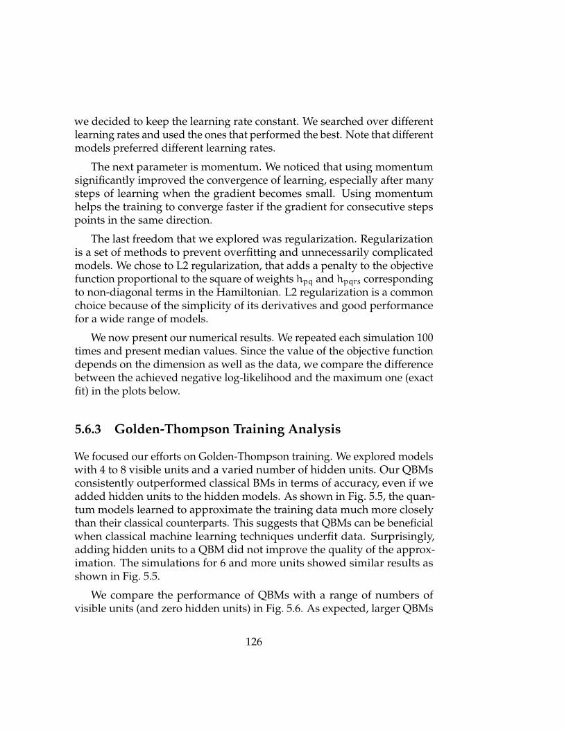
we decided to keep the learning rate constant. We searched over differentlearning rates and used the ones that performed the best. Note that differentmodels preferred different learning rates.
The next parameter is momentum. We noticed that using momentumsignificantly improved the convergence of learning, especially after manysteps of learning when the gradient becomes small. Using momentumhelps the training to converge faster if the gradient for consecutive stepspoints in the same direction.
The last freedom that we explored was regularization. Regularizationis a set of methods to prevent overfitting and unnecessarily complicatedmodels. We chose to L2 regularization, that adds a penalty to the objectivefunction proportional to the square of weights hpq and hpqrs correspondingto non-diagonal terms in the Hamiltonian. L2 regularization is a commonchoice because of the simplicity of its derivatives and good performancefor a wide range of models.
We now present our numerical results. We repeated each simulation 100times and present median values. Since the value of the objective functiondepends on the dimension as well as the data, we compare the differencebetween the achieved negative log-likelihood and the maximum one (exactfit) in the plots below.
5.6.3 Golden-Thompson Training Analysis
We focused our efforts on Golden-Thompson training. We explored modelswith 4 to 8 visible units and a varied number of hidden units. Our QBMsconsistently outperformed classical BMs in terms of accuracy, even if weadded hidden units to the hidden models. As shown in Fig. 5.5, the quan-tum models learned to approximate the training data much more closelythan their classical counterparts. This suggests that QBMs can be beneficialwhen classical machine learning techniques underfit data. Surprisingly,adding hidden units to a QBM did not improve the quality of the approx-imation. The simulations for 6 and more units showed similar results asshown in Fig. 5.5.
We compare the performance of QBMs with a range of numbers ofvisible units (and zero hidden units) in Fig. 5.6. As expected, larger QBMs
126

101 102 103
epoch
0.01
0.1
1
−∆O
Λ(m
edia
n)
q, hidden = 0q, hidden = 1q, hidden = 2c, hidden = 0c, hidden = 1c, hidden = 2
Figure 5.5: Comparison of classical and quantum Boltzmann machines(with Golden-Thompson training) for 5 visible units. This figure firstappeared in [4]. The vertical axis shows the difference between asymptoticvalue of the objective function and the objective function for the learnedmodel in a given epoch.
require longer to learn. We were not able to determine how the complexityof QBM training scales with the number of visible units. Presumably,this can heavily depend on the training data and in some cases growexponentially.
5.6.4 Commutator Training Analysis
We examine the performance of commutator training for an all-visible Boltz-mann machine with 4 visible units and compare it with Golden-Thompsontraining. We immediately noticed that this type of the training is not nu-merically stable. In particular, we were not able to use commutator trainingat all when the learning rate or the gradient were too large – the learning
127
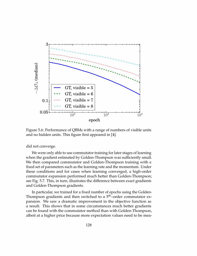
102 103 104
epoch
0.05
0.1
3
−∆O
Λ(m
edia
n)
GT, visible = 5GT, visible = 6GT, visible = 7GT, visible = 8
Figure 5.6: Performance of QBMs with a range of numbers of visible unitsand no hidden units. This figure first appeared in [4].
did not converge.
We were only able to use commutator training for later stages of learningwhen the gradient estimated by Golden-Thompson was sufficiently small.We then compared commutator and Golden-Thompson training with afixed set of parameters such as the learning rate and the momentum. Underthese conditions and for cases when learning converged, a high-ordercommutator expansion performed much better than Golden-Thompson;see Fig. 5.7. This, in turn, illustrates the difference between exact gradientsand Golden-Thompson gradients.
In particular, we trained for a fixed number of epochs using the Golden-Thompson gradients and then switched to a 5th–order commutator ex-pansion. We saw a dramatic improvement in the objective function asa result. This shows that in some circumstances much better gradientscan be found with the commutator method than with Golden-Thompson,albeit at a higher price because more expectation values need to be mea-
128

50 100 200 400
epoch
1.5
1.75
2
2.25
−O
Λ(m
edia
n)
commutator post-trainingcommutator post-trainingcommutator post-trainingoptimized GT training
Figure 5.7: Plot showing the accuracy of commutator training for all-visibleBoltzmann machines with 4 visible units. The top lines depict trainingwith Golden-Thompson at first and then switching to commutator trainingwhere we see a sudden increase in accuracy. We picked the parameters suchthat the commutator training is stable. The bottom line (dashed) showsthe performance of Golden-Thompson training with optimized learningrate and momentum. We always kept the learning rate constant during thetraining; changing the learning rate might improve the learning outcomebut introduces another degree of complexity. This figure first appearedin [4].
sured. In other words the gradients estimated from Golden-Thompson arenot always close to the gradients of the negative log-likelihood (withoutapproximation).
We also noticed that the optimal learning rate for this form of train-ing can substantially differ from the optimal learning rate for Golden-Thompson training. We compared our results from commutator trainingto the results with optimized learning rate for Golden-Thompson training.
129
We found out that the optimized version of Golden-Thompson trainingperformed much better. This version of Golden-Thompson training useda high learning rate that was incompatible with commutator training be-cause of numerical instabilities. As such, we could not find a case whencommutator training proved useful; it only showed an advantage whencompared to highly constrained Golden-Thompson training.
This shows that while commutator training can give more accurategradients, it does not necessarily require fewer gradient steps and its use isvery limited. In practice, the method could be used in the last few trainingepochs after Golden–Thompson training or other forms of approximatetraining to reach a local optimum, but its use is otherwise limited.
5.6.5 Relative Entropy Analysis
We can train the QBM with relative entropy training using the same classicaldata set as POVM training. We successfully reproduce results from GoldenThompson training and find out that two approaches converge similarly;see Fig. 5.8. We were not able to train QBMs with hidden units; however,including hidden units from QBMs was in general unnecessary for oursimple data.
Next, we train our QBM to reconstruct two-qubit states using relativeentropy training. This task demonstrates that QBMs can be used for to-mography. We trained QBMs on both pure and mixed states, and in allcases our model was able to reconstruct these states within graphical ac-curacy (i.e. the learned state is visually indistinguishable from the truestate) in 5 epochs as seen in Fig. 5.9. Since we chose our Hamiltonian toconsist of every two-qubit Pauli operator, we did not need to use hiddenunits. A limitation of this approach was the requirement of all visible units.Wossling and Wiebe [237] recently provided a method for training QBMswith hidden units.
5.7 Conclusion
In this chapter, we proposed methods to train quantum Boltzmann ma-chines on quantum data. We demonstrated that the models can successfully
130

102 103 104 105
epoch
10−2
10−1
−∆O
Λ(m
edia
n)
entropyq, hidden = 0
Figure 5.8: Comparison of performance of a QBM using Golden-ThompsonPOVM training and relative entropy training. In our experiments, the twoapproaches performed similarly. This figure first appeared in [4].
learn under idealized conditions, but more research is needed to prove theusefulness of QBM training.
The first open question is how well QBMs learn under realistic assump-tions. That is, in practice we will not have direct access to thermal states orprecise estimates of expectation values. When training classical BMs, theissue of Gibbs sampling is circumvented by using contrastive divergenceand explicitly computing certain expectation values. It is not clear howmany samples would be required for an accurate estimate of expectationvalues for gradient computation. Also, it would be interesting to explorewhether there is an analog of contrastive divergence for QBM training.
The second question is the inclusion of hidden units for relative entropytraining. Hidden units would be necessary for constructing deep quan-tum Boltzmann machines and for training only with local Hamiltonians.Recently, Wiebe and Wossnig [237] proposed methods for training such
131

432
1 Epochs
143
21
0
0.2
0.4
432
3 Epochs
143
21
0
0.2
0.4
432
5 Epochs
143
21
0
0.2
0.4
4
True Mixed State
32143
21
0
0.2
0.4
432
1 Epochs
143
21
0
0.2
0.4
432
3 Epochs
143
21
0
0.2
0.4
432
5 Epochs
143
21
0
0.2
0.4
4
True Mixed State
32143
21
0
0.2
0.4
432
1 Epochs
143
21
0
0.2
0.4
432
3 Epochs
143
21
0
0.5
1
432
5 Epochs
143
21
0
0.5
1
4
True Pure State
32143
21
0
0.5
1
432
1 Epochs
143
21
0.5
0
432
3 Epochs
143
21
0
0.2
0.4
432
5 Epochs
143
21
0
0.2
0.4
4
True Pure State
32143
21
0
0.2
0.4
Figure 5.9: Absolute values of tomographic reconstruction of two-qubitpure states and mixed states using relative entropy training with learningrate η = 1. This figure first appeared in [4].
QBMs.
We mostly avoided the topic of overfitting data. This is because charac-terizing quantum states is a resource-intensive task and having too muchquantum processing power is not likely to be an issue in the near future.Eventually, we will need to introduce methods to prevent us from learningsampling errors. One such method is L2 regularization that we incorpo-rated in our numerical experiments. It would be interesting to examinehow classical regularization techniques perform in the quantum setting,
132
as well as to develop new overfitting techniques. Additionally, we willeventually need to use separate data for validation of QML algorithms.
Lastly, the most important strength of QBMs is their ability to replacetomography for quantum states with structure. Since we require onlyapproximations of thermal states and computation of expectation values,relative entropy training is near ideally suited for near future experiments.We hope that combining ideas from quantum machine learning, quan-tum Hamiltonian learning, and state estimation will lead to more efficientmethods that will be eventually employed in practice.
133

6Conclusion and Future Work
“Full stories are as rare as honesty.”
Zadie Smith (White Teeth)
In this thesis, we presented several techniques for building efficientquantum algorithms. Our goal was to improve quantum algorithm perfor-mance for practical tasks, such as estimating energies in quantum chemistry.
The first set of techniques, quantum comparison, sort, and shuffle,are presented in Chapter 3 and based on our paper [2]. We developed aquantum shuffle to antisymmetrize fermionic states in first quantizationquickly. The components of one of our shuffling algorithms, comparisonand sort, later found applications in state preparation [116] and simulationof time-independent Hamiltonians [3].
Chapter 4 focused on our algorithm for simulating time-dependentHamiltonians. This algorithm has applications for simulating quantumchemistry with moving nuclei, a digital simulation of adiabatic computa-tion, and simulations in the interaction picture. The next step will be toestimate the resources of using this method for benchmark molecules in
134

quantum chemistry. Calculating gate counts will also determine which oneof our state preparation methods is more efficient.
Our last methods are for generative learning and tomography withquantum Boltzmann machines based on [4]. We demonstrate how to usequantum Boltzmann machines for training on quantum and classical data.We envision that quantum Boltzmann machines can be used for classicaldata that conventional algorithms underfit, or for partial tomography onquantum states.
Throughout this thesis, we raised many open questions. The first oneis what are the resource requirements of our algorithms. We quantifiedour algorithms in terms of their asymptotic scaling or through numericalsimulations for small examples. In particular, it would be interesting to seehow shuffling and truncated Dyson series algorithms perform on quantumchemistry problems. We plan to estimate the explicit gate counts for ourDyson series algorithm in the near future.
In Chapter 5, we showed that we can train quantum Boltzmann ma-chines on quantum data. However, there are many more steps needed toshow that such training is efficient. A method for relative entropy trainingwith hidden units [237] is one such step. Another one is creating approxi-mations of training states, aka quantum contrastive divergence. We willalso need to carefully examine the performance of QBMs with a growingnumber of units. Lastly, it would be interesting to investigate whether cre-ating additional layers and forming a deep quantum Boltzmann machinebrings any advantages.
Lastly, we would like to apply our techniques on a wider array ofproblems. Comparison and sort are simple routines with many applicationsin classical computing and we would like to use our efficient circuits forthem in other quantum algorithms. Similarly, we want to know the scopeof applications of QBMs for tomography, approximate cloning and possiblystate preparation. We hope that the techniques introduced in this thesiswill prove to be widely applicable.
135

References
[1] Yudong Cao, Jonathan Romero, Jonathan P Olson, Matthias Degroote,Peter D Johnson, Maria Kieferova, Ian D Kivlichan, Tim Menke, BorjaPeropadre, Nicolas PD Sawaya, et al. Quantum chemistry in the ageof quantum computing. Chemical Reviews, 2018.
[2] Dominic W Berry, Maria Kieferova, Artur Scherer, Yuval R Sanders,Guang Hao Low, Nathan Wiebe, Craig Gidney, and Ryan Babbush.Improved techniques for preparing eigenstates of fermionic Hamilto-nians. npj Quantum Information, 4:22, 2018.
[3] Maria Kieferova, Artur Scherer, and Dominic W Berry. Simulating thedynamics of time-dependent Hamiltonians with a truncated Dysonseries. Physical Review A, 99(4):042314, 2019.
[4] Maria Kieferova and Nathan Wiebe. Tomography and generativetraining with quantum Boltzmann machines. Physical Review A,96:062327, 2017.
[5] Aram W Harrow, Avinatan Hassidim, and Seth Lloyd. Quantumalgorithm for linear systems of equations. Physical Review Letters,103(15):150502, 2009.
[6] Richard P Feynman. Quantum mechanical computers. Foundations ofPhysics, 16(6):507–531, 1986.
[7] David Deutsch. Quantum theory, the Church–Turing principle andthe universal quantum computer. Proceedings of the Royal Society ofLondon. A. Mathematical and Physical Sciences, 400(1818):97–117, 1985.
136

[8] David Deutsch and Richard Jozsa. Rapid solution of problems byquantum computation. Proceedings of the Royal Society of London SeriesA, 439:553–558, 1992.
[9] Vladimır Cerny. Quantum computers and intractable (NP-complete)computing problems. Physical Review A, 48(1):116, 1993.
[10] Ethan Bernstein and Umesh Vazirani. Quantum complexity theory.SIAM Journal on Computing, 26(5):1411–1473, 1997.
[11] Daniel R Simon. On the power of quantum computation. SIAMJournal on Computing, 26(5):1474–1483, 1997.
[12] Peter W Shor. Polynomial-time algorithms for prime factorizationand discrete logarithms on a quantum computer. SIAM Review,41(2):303–332, 1999.
[13] Seth Lloyd. Universal quantum simulators. Science, 273(5278):1073–1078, 1996.
[14] Lov K Grover. A fast quantum mechanical algorithm for databasesearch. In Proceedings of the Twenty-Eighth Annual ACM Symposium onTheory of Computing, pages 212–219. ACM, 1996.
[15] Mario Szegedy. Quantum speed-up of markov chain based algo-rithms. In 45th Annual IEEE Symposium on Foundations of ComputerScience, pages 32–41. IEEE, 2004.
[16] Andris Ambainis. Quantum walk algorithm for element distinctness.SIAM Journal on Computing, 37(1):210–239, 2007.
[17] Andrew M Childs, Richard Cleve, Enrico Deotto, Edward Farhi, SamGutmann, and Daniel A Spielman. Exponential algorithmic speedupby a quantum walk. In Proceedings of the Thirty-Fifth Annual ACMSymposium on Theory of Computing, pages 59–68. ACM, 2003.
[18] Andrew M Childs and Jeffrey Goldstone. Spatial search by quantumwalk. Physical Review A, 70(2):022314, 2004.
[19] Andrew M Childs. Universal computation by quantum walk. PhysicalReview Letters, 102(18):180501, 2009.
137

[20] Andris Ambainis, Eric Bach, Ashwin Nayak, Ashvin Vishwanath,and John Watrous. One-dimensional quantum walks. In Proceedingsof the Thirty-Third Annual ACM Symposium on Theory of Computing,pages 37–49. ACM, 2001.
[21] Frederic Magniez, Ashwin Nayak, Jeremie Roland, and Miklos San-tha. Search via quantum walk. SIAM Journal on Computing, 40(1):142–164, 2011.
[22] Frederic Magniez, Ashwin Nayak, Peter C Richter, and Miklos Santha.On the hitting times of quantum versus random walks. Algorithmica,63(1-2):91–116, 2012.
[23] Stacey Jeffery, Robin Kothari, and Frederic Magniez. Nested quantumwalks with quantum data structures. In Proceedings of the Twenty-Fourth Annual ACM-SIAM Symposium on Discrete algorithms, pages1474–1485. Society for Industrial and Applied Mathematics, 2013.
[24] Neil B Lovett, Sally Cooper, Matthew Everitt, Matthew Trevers, andViv Kendon. Universal quantum computation using the discrete-timequantum walk. Physical Review A, 81(4):042330, 2010.
[25] Ashley Montanaro. Quantum walk speedup of backtracking algo-rithms. arXiv:1509.02374, 2015.
[26] Andrew M Childs, David Gosset, and Zak Webb. Universal compu-tation by multiparticle quantum walk. Science, 339(6121):791–794,2013.
[27] Andrew M Childs. On the relationship between continuous-anddiscrete-time quantum walk. Communications in Mathematical Physics,294(2):581–603, 2010.
[28] Dorit Aharonov, Wim van Dam, Julia Kempe, Zeph Landau, SethLloyd, and Odev Regev. Adiabatic Quantum Computation is Equiva-lent to Standard Quantum Computation. In 45th Annual IEEE Sympo-sium on Foundations of Computer Science. IEEE, 2004.
[29] Dominic W Berry, Graeme Ahokas, Richard Cleve, and Barry C.Sanders. Efficient quantum algorithms for simulating sparse Hamil-tonians. Communications in Mathematical Physics, 270(2):359–371, 2006.
138

[30] Nathan Wiebe, Dominic Berry, Peter Høyer, and Barry C Sanders.Higher order decompositions of ordered operator exponentials. Jour-nal of Physics A: Mathematical and Theoretical, 43(6):065203, 2010.
[31] Dominic W Berry and Andrew M Childs. Black-box Hamiltoniansimulation and unitary implementation. Quantum Information andComputation, 12:0029–0062, 2012.
[32] Dominic W Berry, Andrew M Childs, and Robin Kothari. Hamilto-nian simulation with nearly optimal dependence on all parameters.In Proceedings of the 56th IEEE Symposium on Foundations of ComputerScience (FOCS), pages 792–809, 2015.
[33] Dominic W Berry, Richard Cleve, and Rolando D Somma. Exponen-tial improvement in precision for Hamiltonian-evolution simulation.arXiv:1308.5424, 2013.
[34] Dominic W Berry, Andrew M Childs, Richard Cleve, Robin Kothari,and Rolando D Somma. Simulating Hamiltonian dynamics with atruncated Taylor series. Physical Review Letters, 114(9):090502, 2015.
[35] Guang Hao Low and Isaac L Chuang. Optimal Hamiltonian simula-tion by quantum signal processing. Physical Review Letters, 118:010501,2017.
[36] Andras Gilyen, Yuan Su, Guang Hao Low, and Nathan Wiebe. Quan-tum singular value transformation and beyond: exponential improve-ments for quantum matrix arithmetics. arXiv:1806.01838, 2018.
[37] Guang Hao Low and Nathan Wiebe. Hamiltonian simulation in theinteraction picture. arXiv:1805.00675, 2018.
[38] Edward Farhi, Jeffrey Goldstone, Sam Gutmann, and Michael Sipser.Quantum computation by adiabatic evolution. arXiv:0001106, 2000.
[39] Wim Van Dam, Michele Mosca, and Umesh Vazirani. How pow-erful is adiabatic quantum computation? In Proceedings 2001 IEEEInternational Conference on Cluster Computing, pages 279–287. IEEE,2001.
139

[40] Andrew M Childs, Edward Farhi, and John Preskill. Robustnessof adiabatic quantum computation. Physical Review A, 65(1):012322,2001.
[41] Jeremie Roland and Nicolas J Cerf. Adiabatic quantum search algo-rithm for structured problems. Physical Review A, 68:62312, 2003.
[42] Tameem Albash and Daniel A Lidar. Adiabatic quantum computa-tion. Reviews of Modern Physics, 90(1):015002, 2018.
[43] Rolando D Somma, Daniel Nagaj, and Maria Kieferova. Quan-tum Speedup by Quantum Annealing. Physical Review Letters,109(5):50501–50506, 2012.
[44] Rolando D Somma, Daniel Nagaj, and Maria Kieferova. Quantumspeedup by quantum annealing. Physical Review Letters, 109(5):050501,2012.
[45] Greg Kuperberg. A subexponential-time quantum algorithm for thedihedral hidden subgroup problem. SIAM Journal on Computing,35(1):170–188, 2005.
[46] Daniel J Bernstein, Stacey Jeffery, Tanja Lange, and Alexander Meurer.Quantum algorithms for the subset-sum problem. In InternationalWorkshop on Post-Quantum Cryptography, pages 16–33. Springer, 2013.
[47] Stephen P Jordan, Keith SM Lee, and John Preskill. Quantum al-gorithms for quantum field theories. Science, 336(6085):1130–1133,2012.
[48] Esteban A Martinez, Christine A Muschik, Philipp Schindler, DanielNigg, Alexander Erhard, Markus Heyl, Philipp Hauke, MarcelloDalmonte, Thomas Monz, Peter Zoller, et al. Real-time dynamics oflattice gauge theories with a few-qubit quantum computer. Nature,534(7608):516, 2016.
[49] Gavin K Brennen, Peter Rohde, Barry C Sanders, and SukhwinderSingh. Multiscale quantum simulation of quantum field theory usingwavelets. Physical Review A, 92(3):032315, 2015.
140
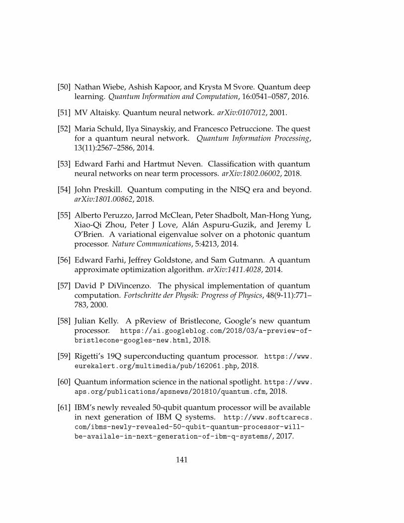
[50] Nathan Wiebe, Ashish Kapoor, and Krysta M Svore. Quantum deeplearning. Quantum Information and Computation, 16:0541–0587, 2016.
[51] MV Altaisky. Quantum neural network. arXiv:0107012, 2001.
[52] Maria Schuld, Ilya Sinayskiy, and Francesco Petruccione. The questfor a quantum neural network. Quantum Information Processing,13(11):2567–2586, 2014.
[53] Edward Farhi and Hartmut Neven. Classification with quantumneural networks on near term processors. arXiv:1802.06002, 2018.
[54] John Preskill. Quantum computing in the NISQ era and beyond.arXiv:1801.00862, 2018.
[55] Alberto Peruzzo, Jarrod McClean, Peter Shadbolt, Man-Hong Yung,Xiao-Qi Zhou, Peter J Love, Alan Aspuru-Guzik, and Jeremy LO’Brien. A variational eigenvalue solver on a photonic quantumprocessor. Nature Communications, 5:4213, 2014.
[56] Edward Farhi, Jeffrey Goldstone, and Sam Gutmann. A quantumapproximate optimization algorithm. arXiv:1411.4028, 2014.
[57] David P DiVincenzo. The physical implementation of quantumcomputation. Fortschritte der Physik: Progress of Physics, 48(9-11):771–783, 2000.
[58] Julian Kelly. A pReview of Bristlecone, Google’s new quantumprocessor. https://ai.googleblog.com/2018/03/a-preview-of-
bristlecone-googles-new.html, 2018.
[59] Rigetti’s 19Q superconducting quantum processor. https://www.
eurekalert.org/multimedia/pub/162061.php, 2018.
[60] Quantum information science in the national spotlight. https://www.aps.org/publications/apsnews/201810/quantum.cfm, 2018.
[61] IBM’s newly revealed 50-qubit quantum processor will be availablein next generation of IBM Q systems. http://www.softcarecs.
com/ibms-newly-revealed-50-qubit-quantum-processor-will-
be-availale-in-next-generation-of-ibm-q-systems/, 2017.
141

[62] Making the world’s first integrated quantum system.https://newsroom.intel.com/wp-content/uploads/sites/11/
2018/05/49-qubit-processor-tangle-lake-infographic.jpg,2018.
[63] Xiaogang Qiang, Xiaoqi Zhou, Jianwei Wang, Callum M Wilkes,Thomas Loke, Sean O’Gara, Laurent Kling, Graham D Marshall,Raffaele Santagati, Timothy C Ralph, et al. Large-scale silicon quan-tum photonics implementing arbitrary two-qubit processing. NaturePhotonics, 12(9):534, 2018.
[64] Making the world’s first integrated quantum system. https://www.research.ibm.com/ibm-q/system-one/, 2019.
[65] Chad Rigetti. The Rigetti 128-qubit chip and what it means forquantum. https://medium.com/rigetti/the-rigetti-128-qubit-chip-and-what-it-means-for-quantum-df757d1b71ea, 2018.
[66] The Rigetti 128-qubit chip and what it means for quantum. https://ionq.co/.
[67] The path to the world’s most powerful quantum computer.https://www.honeywell.com/en-us/newsroom/news/2019/01/the-
path-to-the-world-s-most-powerful-quantum-computer, 2019.
[68] Austin G Fowler, Matteo Mariantoni, John M Martinis, and An-drew N Cleland. Surface codes: Towards practical large-scale quan-tum computation. Physical Review A, 86(3):032324, 2012.
[69] Craig Gidney and Martin Ekera. How to factor 2048 bit RSA integersin 8 hours using 20 million noisy qubits. arXiv:1905.09749, 2019.
[70] Ivan Kassal, Stephen P Jordan, Peter J Love, Masoud Mohseni, andAlan Aspuru-Guzik. Polynomial-time quantum algorithm for thesimulation of chemical dynamics. Proceedings of the National Academyof Sciences, 105(48):18681–18686, 2008.
[71] Alan Aspuru-Guzik, Anthony D Dutoi, Peter J Love, and MartinHead-Gordon. Simulated quantum computation of molecular ener-gies. Science, 309(5741):1704, 2005.
142

[72] Ryan Babbush, Dominic W Berry, Ian D. Kivlichan, Annie Y. Wei,Peter J. Love, and Alan Aspuru-Guzik. Exponentially more precisequantum simulation of fermions in second quantization. New Journalof Physics, 18(3):033032, 2016.
[73] Ryan Babbush, Craig Gidney, Dominic W Berry, Nathan Wiebe, Jar-rod McClean, Alexandru Paler, Austin Fowler, and Hartmut Neven.Encoding electronic spectra in quantum circuits with linear t com-plexity. Physical Review X, 8(4):041015, 2018.
[74] Ryan Babbush, Dominic W Berry, Jarrod R. McClean, and HartmutNeven. Quantum simulation of chemistry with sublinear scaling tothe continuum. arXiv:1807.09802, 2018.
[75] Ronald L Rivest, Adi Shamir, and Leonard Adleman. A method forobtaining digital signatures and public-key cryptosystems. Commu-nications of the ACM, 21(2):120–126, 1978.
[76] Sadegh Raeisi, Maria Kieferova, and Michele Mosca. Novel tech-nique for robust optimal algorithmic cooling. Physical Review Letters,122:220501, Jun 2019.
[77] Maria Kieferova and Nathan Wiebe. On the power of coherentlycontrolled quantum adiabatic evolutions. New Journal of Physics,16(12):123034, 2014.
[78] Scott Aaronson, Greg Kuperberg, and Christopher Granade.The Complexity Zoo. https://complexityzoo.uwaterloo.ca/
Complexity_Zoo, 2005.
[79] Phillip Kaye, Raymond Laflamme, and Michele Mosca. An introduc-tion to quantum computing. Oxford University Press, 2007.
[80] Chris Ferrie. Quantum Computing for Babies. Jabberwocky, 2017.
[81] Michael A. Nielsen and Isaac L. Chuang. Quantum Computation andQuantum Information. Cambridge University Press, 2010.
[82] Stephen Jordan. Quantum Algorithm Zoo. https://math.nist.gov/quantum/zoo/.
143
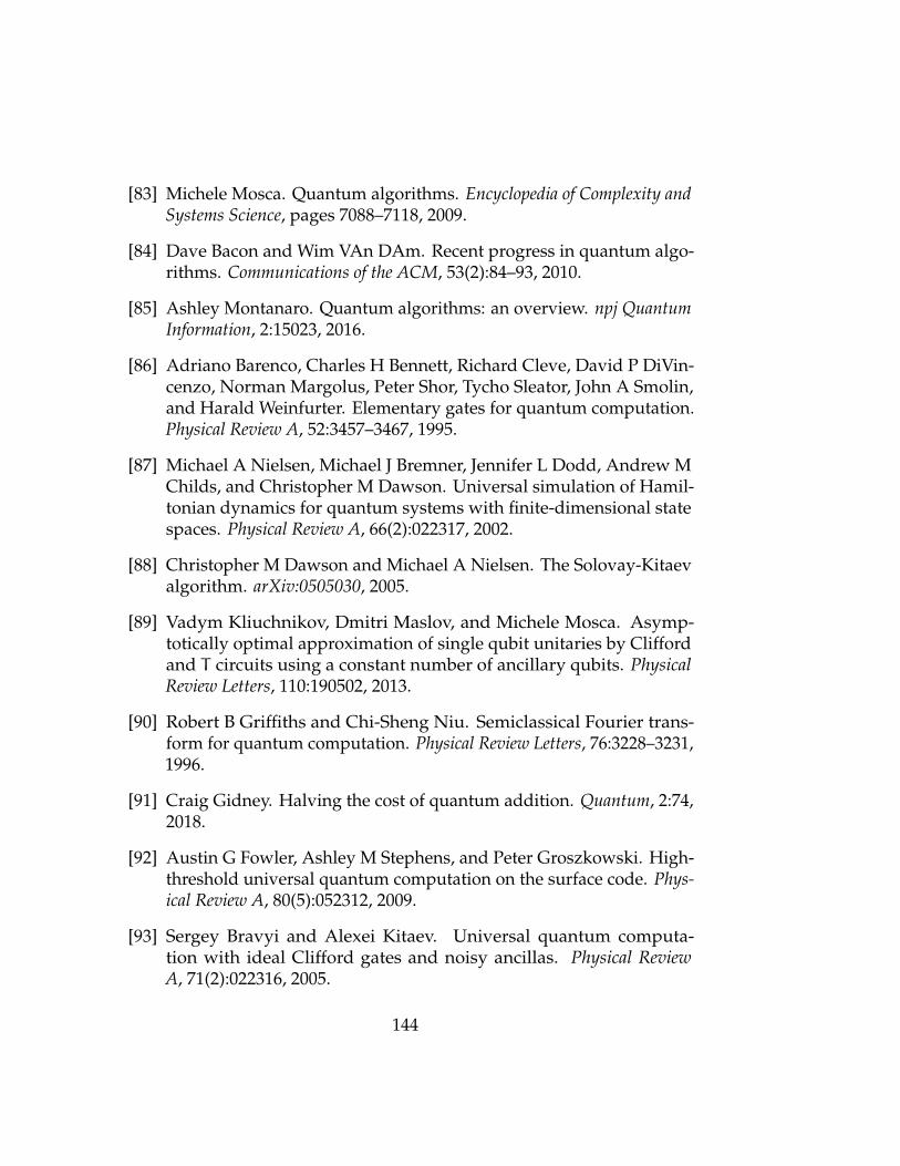
[83] Michele Mosca. Quantum algorithms. Encyclopedia of Complexity andSystems Science, pages 7088–7118, 2009.
[84] Dave Bacon and Wim VAn DAm. Recent progress in quantum algo-rithms. Communications of the ACM, 53(2):84–93, 2010.
[85] Ashley Montanaro. Quantum algorithms: an overview. npj QuantumInformation, 2:15023, 2016.
[86] Adriano Barenco, Charles H Bennett, Richard Cleve, David P DiVin-cenzo, Norman Margolus, Peter Shor, Tycho Sleator, John A Smolin,and Harald Weinfurter. Elementary gates for quantum computation.Physical Review A, 52:3457–3467, 1995.
[87] Michael A Nielsen, Michael J Bremner, Jennifer L Dodd, Andrew MChilds, and Christopher M Dawson. Universal simulation of Hamil-tonian dynamics for quantum systems with finite-dimensional statespaces. Physical Review A, 66(2):022317, 2002.
[88] Christopher M Dawson and Michael A Nielsen. The Solovay-Kitaevalgorithm. arXiv:0505030, 2005.
[89] Vadym Kliuchnikov, Dmitri Maslov, and Michele Mosca. Asymp-totically optimal approximation of single qubit unitaries by Cliffordand T circuits using a constant number of ancillary qubits. PhysicalReview Letters, 110:190502, 2013.
[90] Robert B Griffiths and Chi-Sheng Niu. Semiclassical Fourier trans-form for quantum computation. Physical Review Letters, 76:3228–3231,1996.
[91] Craig Gidney. Halving the cost of quantum addition. Quantum, 2:74,2018.
[92] Austin G Fowler, Ashley M Stephens, and Peter Groszkowski. High-threshold universal quantum computation on the surface code. Phys-ical Review A, 80(5):052312, 2009.
[93] Sergey Bravyi and Alexei Kitaev. Universal quantum computa-tion with ideal Clifford gates and noisy ancillas. Physical ReviewA, 71(2):022316, 2005.
144

[94] Daniel Gottesman. Stabilizer codes and quantum error correction.arXiv:9705052, 1997.
[95] Larry J Stockmeyer. The polynomial-time hierarchy. Theoretical Com-puter Science, 3(1):1–22, 1976.
[96] Dorit Aharonov and Michael Ben-Or. Fault-tolerant quantum com-putation with constant error rate. arxiv:9906129, 1999.
[97] Daniel Gottesman. An introduction to quantum error correction andfault-tolerant quantum computation. In Quantum information scienceand its contributions to mathematics, Proceedings of Symposia in AppliedMathematics, volume 68, pages 13–58, 2010.
[98] Yuval R Sanders, Joel J Wallman, and Barry C Sanders. Boundingquantum gate error rate based on reported average fidelity. NewJournal of Physics, 18(1):012002, 2015.
[99] John Preskill. Sufficient condition on noise correlations for scalablequantum computing. arXiv:1207.6131, 2012.
[100] Gil Kalai. Quantum computers: noise propagation and adversarialnoise models. arXiv:0904.3265, 2009.
[101] Peter W Shor. Scheme for reducing decoherence in quantum com-puter memory. Physical Review A, 52:R2493–R2496, 1995.
[102] Chenyang Wang, Jim Harrington, and John Preskill. Confinement-Higgs transition in a disordered gauge theory and the accuracythreshold for quantum memory. Annals of Physics, 303(1):31–58, 2003.
[103] Michael Freedman, Alexei Y Kitaev, Michael Larsen, and ZhenghanWang. Topological quantum computation. Bulletin of the AmericanMathematical Society, 40(1):31–38, 2003.
[104] Sergey B Bravyi and Alexei Y Kitaev. Quantum codes on a latticewith boundary. arXiv:9811052, 1998.
[105] Eric Dennis, Alexei Kitaev, Andrew Landahl, and John Preskill. Topo-logical quantum memory. Journal of Mathematical Physics, 43(9):4452–4505, 2002.
145

[106] Tommaso Toffoli. Reversible computing. In International Colloquiumon Automata, Languages, and Programming, pages 632–644. Springer,1980.
[107] Edward Fredkin and Tommaso Toffoli. Conservative logic. Interna-tional Journal of Theoretical Physics, 21(3-4):219–253, 1982.
[108] Rolf Landauer. Irreversibility and heat generation in the computingprocess. IBM Journal of Research and Development, 5(3):183–191, 1961.
[109] Charles H Bennett. Notes on the history of reversible computation.ibm Journal of Research and Development, 32(1):16–23, 1988.
[110] Charles H Bennett. Notes on Landauer’s principle, reversible com-putation, and Maxwell’s Demon. Studies In History and Philosophyof Science Part B: Studies In History and Philosophy of Modern Physics,34(3):501–510, 2003.
[111] Alex Parent, Martin Roetteler, and Michele Mosca. Improved re-versible and quantum circuits for Karatsuba-based integer multipli-cation. arXiv:1706.03419, 2017.
[112] Vivek V Shende, Aditya K Prasad, Igor L Markov, and John P Hayes.Synthesis of reversible logic circuits. IEEE Transactions on Computer-Aided Design of Integrated Circuits and Systems, 22(6):710–722, 2003.
[113] Mehdi Saeedi and Igor L Markov. Synthesis and optimization ofreversible circuits–a survey. ACM Computing Surveys (CSUR), 45(2):21,2013.
[114] D Michael Miller, Dmitri Maslov, and Gerhard W Dueck. A transfor-mation based algorithm for reversible logic synthesis. In Proceedings2003. Design Automation Conference (IEEE Cat. No. 03CH37451), pages318–323. IEEE, 2003.
[115] Mathias Soeken, Martin Roetteler, Nathan Wiebe, and Gio-vanni De Micheli. Logic synthesis for quantum computing.arXiv:1706.02721, 2017.
[116] Yuval R Sanders, Guang Hao Low, Artur Scherer, and Dominic WBerry. Black-box quantum state preparation without arithmetic. Phys-ical Review Letters, 122:020502, 2019.
146
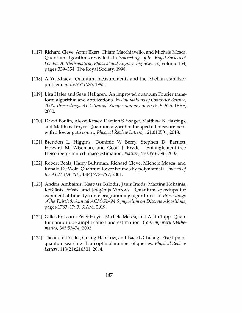
[117] Richard Cleve, Artur Ekert, Chiara Macchiavello, and Michele Mosca.Quantum algorithms revisited. In Proceedings of the Royal Society ofLondon A: Mathematical, Physical and Engineering Sciences, volume 454,pages 339–354. The Royal Society, 1998.
[118] A Yu Kitaev. Quantum measurements and the Abelian stabilizerproblem. arxiv:9511026, 1995.
[119] Lisa Hales and Sean Hallgren. An improved quantum Fourier trans-form algorithm and applications. In Foundations of Computer Science,2000. Proceedings. 41st Annual Symposium on, pages 515–525. IEEE,2000.
[120] David Poulin, Alexei Kitaev, Damian S. Steiger, Matthew B. Hastings,and Matthias Troyer. Quantum algorithm for spectral measurementwith a lower gate count. Physical Review Letters, 121:010501, 2018.
[121] Brendon L. Higgins, Dominic W Berry, Stephen D. Bartlett,Howard M. Wiseman, and Geoff J. Pryde. Entanglement-freeHeisenberg-limited phase estimation. Nature, 450:393–396, 2007.
[122] Robert Beals, Harry Buhrman, Richard Cleve, Michele Mosca, andRonald De Wolf. Quantum lower bounds by polynomials. Journal ofthe ACM (JACM), 48(4):778–797, 2001.
[123] Andris Ambainis, Kaspars Balodis, Janis Iraids, Martins Kokainis,Krisjanis Prusis, and Jevgenijs Vihrovs. Quantum speedups forexponential-time dynamic programming algorithms. In Proceedingsof the Thirtieth Annual ACM-SIAM Symposium on Discrete Algorithms,pages 1783–1793. SIAM, 2019.
[124] Gilles Brassard, Peter Hoyer, Michele Mosca, and Alain Tapp. Quan-tum amplitude amplification and estimation. Contemporary Mathe-matics, 305:53–74, 2002.
[125] Theodore J Yoder, Guang Hao Low, and Isaac L Chuang. Fixed-pointquantum search with an optimal number of queries. Physical ReviewLetters, 113(21):210501, 2014.
147
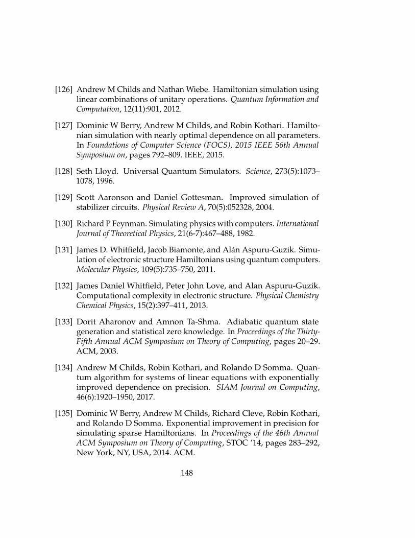
[126] Andrew M Childs and Nathan Wiebe. Hamiltonian simulation usinglinear combinations of unitary operations. Quantum Information andComputation, 12(11):901, 2012.
[127] Dominic W Berry, Andrew M Childs, and Robin Kothari. Hamilto-nian simulation with nearly optimal dependence on all parameters.In Foundations of Computer Science (FOCS), 2015 IEEE 56th AnnualSymposium on, pages 792–809. IEEE, 2015.
[128] Seth Lloyd. Universal Quantum Simulators. Science, 273(5):1073–1078, 1996.
[129] Scott Aaronson and Daniel Gottesman. Improved simulation ofstabilizer circuits. Physical Review A, 70(5):052328, 2004.
[130] Richard P Feynman. Simulating physics with computers. InternationalJournal of Theoretical Physics, 21(6-7):467–488, 1982.
[131] James D. Whitfield, Jacob Biamonte, and Alan Aspuru-Guzik. Simu-lation of electronic structure Hamiltonians using quantum computers.Molecular Physics, 109(5):735–750, 2011.
[132] James Daniel Whitfield, Peter John Love, and Alan Aspuru-Guzik.Computational complexity in electronic structure. Physical ChemistryChemical Physics, 15(2):397–411, 2013.
[133] Dorit Aharonov and Amnon Ta-Shma. Adiabatic quantum stategeneration and statistical zero knowledge. In Proceedings of the Thirty-Fifth Annual ACM Symposium on Theory of Computing, pages 20–29.ACM, 2003.
[134] Andrew M Childs, Robin Kothari, and Rolando D Somma. Quan-tum algorithm for systems of linear equations with exponentiallyimproved dependence on precision. SIAM Journal on Computing,46(6):1920–1950, 2017.
[135] Dominic W Berry, Andrew M Childs, Richard Cleve, Robin Kothari,and Rolando D Somma. Exponential improvement in precision forsimulating sparse Hamiltonians. In Proceedings of the 46th AnnualACM Symposium on Theory of Computing, STOC ’14, pages 283–292,New York, NY, USA, 2014. ACM.
148

[136] Dominic W Berry, Richard Cleve, and Sevag Gharibian. Gate-efficientdiscrete simulations of continuous-time quantum query algorithms.Quantum Information & Computation, 14(1-2):1–30, 2014.
[137] Guang Hao Low and Isaac L Chuang. Hamiltonian simulation byqubitization. Quantum, 3:163, 2019.
[138] Dominic W. Berry, Graeme Ahokas, Richard Cleve, and Barry C.Sanders. Quantum Algorithms for Hamiltonian Simulation. In LouisKauffman and Samuel J. Lomonaco, editors, Mathematics of QuantumComputation and Quantum Technology, Chapman & Hall/CRC AppliedMathematics & Nonlinear Science, pages 89–112. CRC Press, 2007.
[139] I M Georgescu, S Ashhab, and Franco Nori. Quantum simulation.Reviews of Modern Physics, 86(1):153–185, 2014.
[140] A. Aspuru-Guzik, A. Dutoi, P. J. Love, and M. Head-Gordon.Simulated quantum computation of molecular energies. Science,309(5741):1704–1707, 2005.
[141] Seth Lloyd, Masoud Mohseni, and Patrick Rebentrost. Quantumprincipal component analysis. Nature Physics, 10:631–633, 2014.
[142] Robert Beals, Stephen Brierley, Oliver Gray, Aram W Harrow, SamuelKutin, Noah Linden, Dan Shepherd, and Mark Stather. Efficientdistributed quantum computing. Proceedings of the Royal Society A,469(2153), 2013.
[143] Edward Farhi, Jeffrey Goldstone, Sam Gutmann, and Michael Sipser.Limit on the speed of quantum computation in determining parity.Physical Review Letters, 81(24):5442, 1998.
[144] Andrew M Childs and Robin Kothari. Limitations on the simulationof non-sparse Hamiltonians. arXiv:0908.4398, 2009.
[145] Jeongwan Haah, Matthew Hastings, Robin Kothari, and Guang HaoLow. Quantum algorithm for simulating real time evolution of latticehamiltonians. In 2018 IEEE 59th Annual Symposium on Foundations ofComputer Science (FOCS), pages 350–360. IEEE, 2018.
149

[146] Masuo Suzuki. Fractal decomposition of exponential operators withapplications to many-body theories and Monte Carlo simulations.Physics Letters A, 146(6):319–323, 1990.
[147] Andrew M Childs, Dmitri Maslov, Yunseong Nam, Neil J Ross,and Yuan Su. Toward the first quantum simulation with quantumspeedup. Proceedings of the National Academy of Sciences, 115(38):9456–9461, 2018.
[148] Andrew M Childs, Aaron Ostrander, and Yuan Su. Faster quantumsimulation by randomization. Quantum, 3:182, 2019.
[149] Earl Campbell. Random compiler for fast hamiltonian simulation.Physical Review Letters, 123(7):070503, 2019.
[150] Andrew M Childs. Quantum information processing in continuous time.PhD thesis, Massachusetts Institute of Technology, 2004.
[151] Andrew M Childs and Robin Kothari. Simulating sparse Hamiltoni-ans with star decompositions. In Conference on Quantum Computation,Communication, and Cryptography, pages 94–103. Springer, 2010.
[152] Andrew M Childs, Edward Farhi, and Sam Gutmann. An exam-ple of the difference between quantum and classical random walks.Quantum Information Processing, 1(1):35–43, 2002.
[153] Andris Ambainis, Andrew M Childs, Ben W Reichardt, Robert Spalek,and Shengyu Zhang. Any AND-OR formula of size N can be eval-uated in time N1/2+o(1) on a quantum computer. SIAM Journal onComputing, 39(6):2513–2530, 2010.
[154] Stacey Jeffery. Frameworks for Quantum Algorithms. PhD thesis, Uni-versity of Waterloo, 2014.
[155] Andris Ambainis. Quantum walks and their algorithmic applications.International Journal of Quantum Information, 1(04):507–518, 2003.
[156] Harry Buhrman, Christoph Durr, Mark Heiligman, Peter Hoyer,Frederic Magniez, Miklos Santha, and Ronald De Wolf. Quantumalgorithms for element distinctness. In Computational Complexity, 16thAnnual IEEE Conference on, 2001., pages 131–137. IEEE, 2001.
150

[157] Chen-Fu Chiang, Daniel Nagaj, and Pawel Wocjan. Efficient circuitsfor quantum walks. arXiv:0903.3465, 2009.
[158] T Loke and JB Wang. Efficient quantum circuits for szegedy quantumwalks. Annals of Physics, 382:64–84, 2017.
[159] Leonardo Novo and Dominic W Berry. Improved Hamiltonian simu-lation via a truncated Taylor series and corrections. arXiv: 1611.10033,2016.
[160] Guang Hao Low, Theodore J Yoder, and Isaac L Chuang. Method-ology of resonant equiangular composite quantum gates. PhysicalReview X, 6:041067, 2016.
[161] Nathan Wiebe, Dominic W Berry, Peter Høyer, and Barry C Sanders.Simulating quantum dynamics on a quantum computer. Journal ofPhysics A: Mathematical and Theoretical, 44(44):445308, 2011.
[162] David Poulin, Angie Qarry, Rolando Somma, and Frank Verstraete.Quantum simulation of time-dependent Hamiltonians and the con-venient illusion of Hilbert space. Physical Review Letters, 106:170501,2011.
[163] David Poulin, Angie Qarry, Rolando Somma, and Frank Verstraete.Quantum simulation of time-dependent Hamiltonians and the conve-nient illusion of hilbert space. Physical Review Letters, 106(17):170501,2011.
[164] W Forrest Stinespring. Positive functions on C*-algebras. Proceedingsof the American Mathematical Society, 6(2):211–216, 1955.
[165] Martin Kliesch, Thomas Barthel, Christian Gogolin, Michael Kasto-ryano, and Jens Eisert. Dissipative quantum Church-Turing theorem.Physical Review Letters, 107(12):120501, 2011.
[166] Andrew M Childs and Tongyang Li. Efficient simulation of sparsemarkovian quantum dynamics. arXiv:1611.05543, 2016.
[167] Richard Cleve and Chunhao Wang. Efficient quantum algorithms forsimulating Lindblad evolution. arXiv:1612.09512, 2016.
151
[168] Richard Durstenfeld. Algorithm 235: random permutation. Commu-nications of the ACM, 7(7):420, 1964.
[169] Donald Ervin Knuth. The art of computer programming, volume 3.Pearson Education, 1997.
[170] Daniel S Abrams and Seth Lloyd. Quantum algorithm providingexponential speed increase for finding eigenvalues and eigenvectors.Physical Review Letters, 83(2):5162–5165, 1999.
[171] Sorting network entry on Wikipedia. https://en.wikipedia.org/wiki/Sorting_network. Accessed: 2019-04-17.
[172] Sheng-Tzong Cheng and Chun-Yen Wang. Quantum switching andquantum merge sorting. IEEE Transactions on Circuits and Systems I:Regular Papers, 53(2):316–325, 2006.
[173] Michael J. Bremner, Ashley Montanaro, and Dan J. Shepherd. Achiev-ing quantum supremacy with sparse and noisy commuting quantumcomputations. Quantum, 1:8, April 2017.
[174] K E Batcher. Sorting networks and their applications. Communicationsof the ACM, 32:307–314, 1968.
[175] K J Liszka and K E Batcher. A generalized bitonic sorting network.International Conference on Parallel Processing, 1:105–108, 1993.
[176] M Ajtai, J Komlos, and E Szemeredi. An O(N logN) sorting network.In Proceedings of the Fifteenth Annual ACM Symposium on Theory ofComputing, STOC ’83, pages 1–9, New York, NY, USA, 1983. ACM.
[177] M S Paterson. Improved sorting networks with O(logN) depth.Algorithmica, 5:75–92, 1990.
[178] Michael T Goodrich. Zig-zag sort: A simple deterministic data-oblivious sorting algorithm running in O(N logN) time. In Proceed-ings of the Forty-sixth Annual ACM Symposium on Theory of Computing,STOC ’14, pages 684–693, New York, NY, USA, 2014. ACM.
[179] Michael Codish, Lus Cruz-Filipe, Thorsten Ehlers, Mike Muller, andPeter Schneider-Kamp. Sorting networks: To the end and back again.Journal of Computer and System Sciences, 2016.
152

[180] Cody Jones. Low-overhead constructions for the fault-tolerant Toffoligate. Physical Review A, 87(2):022328, 2013.
[181] Thomas G Draper, Samuel A Kutin, Eric M Rains, and Krysta M Svore.A logarithmic-depth quantum carry-lookahead adder. arXiv:0406142,2004.
[182] Mihir Bellare, Joe Kilian, and Phillip Rogaway. The security of the ci-pher block chaining message authentication code. Journal of Computerand System Sciences, 61(3):362 – 399, 2000.
[183] Daniel S Abrams and Seth Lloyd. Simulation of many-body Fermisystems on a universal quantum computer. Physical Review Letters,79:2586–2589, 1997.
[184] Donny Cheung, Peter Høyer, and Nathan Wiebe. Improved errorbounds for the adiabatic approximation. Journal of Physics A: Mathe-matical and Theoretical, 44(41):415302, 2011.
[185] Edward Farhi, Jeffrey Goldstone, Sam Gutmann, and Michael Sipser.Quantum computation by adiabatic evolution. arXiv:0001106, 2000.
[186] Edward Farhi, Jeffrey Goldstone, Sam Gutmann, and Michael Sipser.Quantum Computation by Adiabatic Evolution. MIT-CTP-2936, 2000.
[187] Donny Cheung, Peter Hoyer, and Nathan Wiebe. Improved errorbounds for the adiabatic approximation. Journal of Physics A: Mathe-matical and Theoretical, 44(41):415302, 2011.
[188] Dominic W Berry, Andrew M Childs, Yuan Su, Xin Wang, and NathanWiebe. Time-dependent Hamiltonian simulation with L1-norm scal-ing. arXiv:1906.07115, 2019.
[189] Geoffrey Hinton, Li Deng, Dong Yu, George Dahl, Abdel-rahman Mo-hamed, Navdeep Jaitly, Andrew Senior, Vincent Vanhoucke, PatrickNguyen, Brian Kingsbury, et al. Deep neural networks for acousticmodeling in speech recognition. IEEE Signal Processing Magazine, 29,2012.
[190] George E Dahl, Dong Yu, Li Deng, and Alex Acero. Context-dependent pre-trained deep neural networks for large-vocabulary
153

speech recognition. IEEE Transactions on Audio, Speech, and LanguageProcessing, 20(1):30–42, 2012.
[191] Alex Graves, Abdel-rahman Mohamed, and Geoffrey Hinton. Speechrecognition with deep recurrent neural networks. In 2013 IEEE In-ternational Conference on Acoustics, Speech and Signal Processing, pages6645–6649. IEEE, 2013.
[192] Simon J D Prince. Computer vision: models, learning, and inference.Cambridge University Press, 2012.
[193] Edward Rosten and Tom Drummond. Machine learning for high-speed corner detection. In European conference on computer vision,pages 430–443. Springer, 2006.
[194] Christian Szegedy, Vincent Vanhoucke, Sergey Ioffe, Jon Shlens, andZbigniew Wojna. Rethinking the inception architecture for computervision. In Proceedings of the IEEE Conference on Computer Vision andPattern Recognition, pages 2818–2826, 2016.
[195] David Silver, Aja Huang, Chris J Maddison, Arthur Guez, Lau-rent Sifre, George Van Den Driessche, Julian Schrittwieser, IoannisAntonoglou, Veda Panneershelvam, Marc Lanctot, et al. Masteringthe game of Go with deep neural networks and tree search. Nature,529(7587):484, 2016.
[196] David Silver, Julian Schrittwieser, Karen Simonyan, IoannisAntonoglou, Aja Huang, Arthur Guez, Thomas Hubert, Lucas Baker,Matthew Lai, Adrian Bolton, et al. Mastering the game of go withouthuman knowledge. Nature, 550(7676):354, 2017.
[197] Yutian Chen, Aja Huang, Ziyu Wang, Ioannis Antonoglou, JulianSchrittwieser, David Silver, and Nando de Freitas. Bayesian optimiza-tion in alphago. arXiv:1812.06855, 2018.
[198] Juan Carrasquilla and Roger G Melko. Machine learning phases ofmatter. Nature Physics, 13(5):431, 2017.
[199] Sandeep Mavadia, Virginia Frey, Jarrah Sastrawan, Stephen Dona,and Michael J Biercuk. Prediction and real-time compensation of
154

qubit decoherence via machine learning. Nature Communications,8:14106, 2017.
[200] Raban Iten, Tony Metger, Henrik Wilming, Lıdia Del Rio, and Re-nato Renner. Discovering physical concepts with neural networks.arXiv:1807.10300, 2018.
[201] Patrick Rebentrost, Masoud Mohseni, and Seth Lloyd. Quantumsupport vector machine for big data classification. Physical ReviewLetters, 113(13):130503, 2014.
[202] Esma Aımeur, Gilles Brassard, and Sebastien Gambs. Machine learn-ing in a quantum world. Advances in Artificial Intelligence, pages431–442, 2006.
[203] Nathan Wiebe, Ashish Kapoor, and Krysta M Svore. Quantumnearest-neighbor algorithms for machine learning. Quantum Informa-tion and Computation, 15, 2018.
[204] Kristen L Pudenz and Daniel A Lidar. Quantum adiabatic machinelearning. Quantum Information Processing, 12(5):2027–2070, 2013.
[205] Hartmut Neven, Vasil S Denchev, Geordie Rose, and William GMacready. Training a binary classifier with the quantum adiabaticalgorithm. arXiv:0811.0416, 2008.
[206] Patrick Rebentrost, Maria Schuld, Francesco Petruccione, and SethLloyd. Quantum gradient descent and Newton’s method for con-strained polynomial optimization. arXiv:1612.01789, 2016.
[207] Nathan Wiebe, Ashish Kapoor, and Krysta M Svore. Quantum per-ceptron models. arXiv:1602.04799, 2016.
[208] Iordanis Kerenidis and Anupam Prakash. Quantum recommendationsystems. arXiv:1603.08675, 2016.
[209] Alex Monras, Gael Sentıs, and Peter Wittek. Inductive supervisedquantum learning. Physical Review Letters, 118(19):190503, 2017.
[210] Maria Schuld, Ilya Sinayskiy, and Francesco Petruccione. Predictionby linear regression on a quantum computer. Physical Review A,94(2):022342, 2016.
155
[211] Vittorio Giovannetti, Seth Lloyd, and Lorenzo Maccone. Quantumrandom access memory. Physical Review Letters, 100(16):160501, 2008.
[212] Vittorio Giovannetti, Seth Lloyd, and Lorenzo Maccone. Architec-tures for a quantum random access memory. Physical Review A,78(5):052310, 2008.
[213] Srinivasan Arunachalam, Vlad Gheorghiu, Tomas Jochym-O’Connor,Michele Mosca, and Priyaa Varshinee Srinivasan. On the robust-ness of bucket brigade quantum RAM. New Journal of Physics,17(12):123010, 2015.
[214] Christopher E Granade, Christopher Ferrie, Nathan Wiebe, andDavid G Cory. Robust online Hamiltonian learning. New Journal ofPhysics, 14(10):103013, 2012.
[215] Jianwei Wang, Stefano Paesani, Raffaele Santagati, Sebastian Knauer,Antonio A Gentile, Nathan Wiebe, Maurangelo Petruzzella, Jeremy LO’Brien, John G Rarity, Anthony Laing, et al. Experimental quantumHamiltonian learning. Nature Physics, 13(6):551, 2017.
[216] Geoffrey E Hinton. Training products of experts by minimizingcontrastive divergence. Neural Computation, 14(8):1771–1800, 2002.
[217] Geoffrey Hinton. Boltzmann machines. Encyclopedia of MachineLearning and Data Mining, pages 1–7, 2014.
[218] Miguel A Carreira-Perpinan and Geoffrey E Hinton. On contrastivedivergence learning. In AISTATS, 2005.
[219] Geoffrey E Hinton and Terrence J Sejnowski. Analyzing cooperativecomputation. In Proceeding of the 5th Annual Congress of the CognitiveScience Society, 1983.
[220] Radford M Neal. Connectionist learning of belief networks. ArtificialIntelligence, 56(1):71–113, 1992.
[221] David H Ackley, Geoffrey E Hinton, and Terrence J Sejnowski.A learning algorithm for boltzmann machines. Cognitive Science,9(1):147–169, 1985.
156

[222] Ruslan Salakhutdinov and Geoffrey Hinton. Deep Boltzmann ma-chines. In Artificial Intelligence and Statistics, pages 448–455, 2009.
[223] Nitish Srivastava and Ruslan R Salakhutdinov. Multimodal learningwith deep boltzmann machines. In Advances in neural informationprocessing systems, pages 2222–2230, 2012.
[224] Geoffrey Hinton. A practical guide to training restricted Boltzmannmachines. Momentum, 9(1):926, 2010.
[225] Mohammad H Amin, Evgeny Andriyash, Jason Rolfe, BohdanKulchytskyy, and Roger Melko. Quantum Boltzmann machine. Phys-ical Review X, 8(2):021050, 2018.
[226] David Poulin and Pawel Wocjan. Sampling from the thermal quan-tum Gibbs state and evaluating partition functions with a quantumcomputer. Physical Review Letters, 103(22):220502, 2009.
[227] Man-Hong Yung and Alan Aspuru-Guzik. A quantum–quantumMetropolis algorithm. Proceedings of the National Academy of Sciences,109(3):754–759, 2012.
[228] Nathan Wiebe, Ashish Kapoor, Christopher Granade, and Krysta MSvore. Quantum inspired training for Boltzmann machines.arXiv:1507.02642, 2015.
[229] Anirban Narayan Chowdhury and Rolando D Somma. Quan-tum algorithms for Gibbs sampling and hitting-time estimation.arXiv:1603.02940, 2016.
[230] Eric R Anschuetz and Yudong Cao. Realizing quantum Boltzmannmachines through eigenstate thermalization. arXiv:1903.01359, 2019.
[231] J M Deutsch. Quantum statistical mechanics in a closed system.Physical Review A, 43:2046–2049, 1991.
[232] Mark Srednicki. Chaos and quantum thermalization. Physical ReviewE, 50:888–901, 1994.
[233] Misha Denil and Nando De Freitas. Toward the implementationof a quantum rbm. In NIPS Deep Learning and Unsupervised FeatureLearning Workshop, volume 5, 2011.
157
[234] Guillaume Verdon, Michael Broughton, and Jacob Biamonte. A quan-tum algorithm to train neural networks using low-depth circuits.arXiv:1712.05304, 2017.
[235] Jingxiang Wu and Timothy H Hsieh. Variational thermal quantumsimulation via thermofield double states. arXiv:1811.11756, 2018.
[236] James D Whitfield, Jacob Biamonte, and Alan Aspuru-Guzik. Simula-tion of electronic structure Hamiltonians using quantum computers.Molecular Physics, 2011.
[237] Nathan Wiebe and Leonard Wossnig. Generative training of quantumBoltzmann machines with hidden units. arXiv:1905.09902, 2019.
[238] Sandhya Samarasinghe. Neural networks for applied sciences and engi-neering: from fundamentals to complex pattern recognition. Auerbachpublications, 2016.
[239] Mohamad H Hassoun et al. Fundamentals of artificial neural networks.MIT press, 1995.
[240] Geoffrey Hinton. Neural networks and machine learning. https:
//www.cs.toronto.edu/~hinton/coursera_lectures.html.
158

AA Brief Introduction To Machine
Learning
Let us briefly introduce a few classical ML concepts that are essential for ourwork. ML algorithms can be divided into supervised, unsupervised, andreinforcement learning. In supervised learning, an algorithm has access toa database of examples with labels. Given enough training, the algorithmis then expected to assign correct labels to new data.
Our algorithm is an unsupervised one, which means that it gets onlya set of data with no labels. A canonical example of an unsupervisedalgorithm is clustering. The goal of the clustering algorithm is to group“similar data” together and divide the data set into two or more clusters.For example, a clustering algorithm can take a set of hand-written digitsand divide them into ten groups, one for each digit (without labels). In-tuitively, the algorithm learns a model that accurately represents the data.Reinforcement learning is a cross between supervised and unsupervisedlearning and is not relevant to this thesis.
159

A1 Generative Modelling
Machine learning algorithms can also be divided into discriminative andgenerative. In a discriminative model, the algorithm learns how to classifythe training samples (represented as binary vectors). After such an algo-rithm is trained, it is supposed to assign each vector to a group of “similar”vectors. In contrast, a generative algorithm learns a model that generatesthe training data. In this setting, the training data are seen as samples froman underlying distribution. A properly trained generative algorithm can beused for sampling from this distribution and to generate examples similarto the training data as in Fig. A.1.
Figure A.1: An example of generative modelling from [222]. The exampleson the left were used to train a deep Boltzmann machine (a restrictedBoltzmann machine with multiple layers). Then, the algorithm generatedthe images on the right-hand side.
If the model is not rich enough, it can underfit the data, i.e. not captureimportant properties of the distribution. Such a model can neither fit thetraining data nor generate new data.
In the other extreme, the model can also overfit data – capture anysampling errors. Such a model appears to perform very well on trainingdata – indeed, we can fit any data perfectly given enough parameters, but
160
it will not generalize. We demonstrate the problem of underfitting andoverfitting on an example in Fig. A.2.
A2 Artificial Neural Networks
Artificial neural networks (and their variants, deep nets) emerged as oneof the main ML tools. We will now briefly review them and introduce theterminology used in this chapter. Artificial neural networks are an MLframework inspired by biology. In biological neural networks, neuronsconnected by synapses are responsible for the activity in animals’ andhumans’ brains.
An artificial neural network (from now on referred to only as a neuralnetwork or ANN) is defined by its graph. The vertices of the graph (alsocalled units) represent neurons and store information as +1 or −1 states1.Some of the units also serve as input or output of the algorithms, and theseare called visible units. Remaining units are referred to as hidden units andcan provide additional complexity to the network. The edges of the graphrepresent connections between units and encode the relationship betweenthe bits of the information. In addition, one can define functions on thisgraph, such as the activation function or the energy function, that specifieshow the information propagates through the network.
It is possible to distinguish two types of ANNs based on the propertiesof the underlying graph structure. Oriented graphs correspond to feed-forward networks, where the information flows only in one direction, andthe graphs do not include cycles. Their counterparts are recurrent neuralnetworks that can include loops and undirected graphs.
From the physics perspective, neural networks with undirected graphsare particularly interesting because they allow defining “energy” as a bilin-ear function
E(x) = xTWx, (A.1)
where W is the adjacency matrix of the graph and the binary vector x isdefined on the units. A Boltzmann machine is an example of a neural
1Machine learning literature often prefers to use 0 and 1, but the notations are equiva-lent.
161
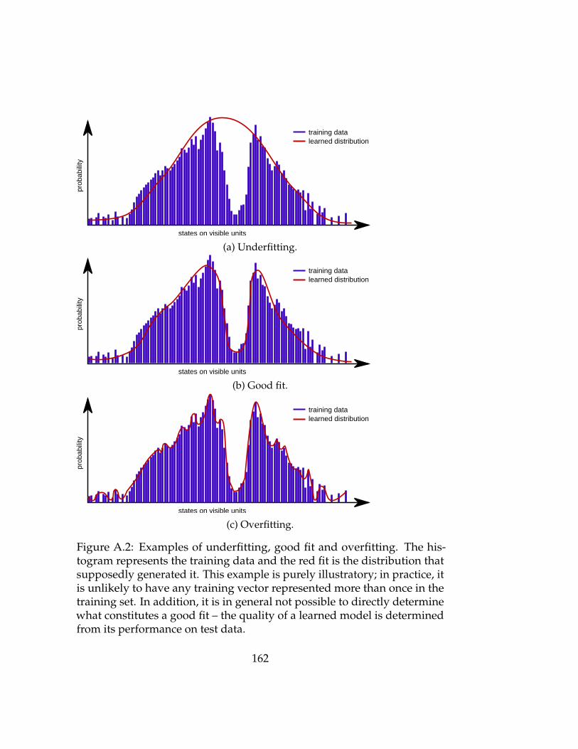
prob
abi
lity
states on visible units
training datalearned distribution
(a) Underfitting.
prob
abi
lity
states on visible units
training datalearned distribution
(b) Good fit.
prob
abi
lity
states on visible units
training datalearned distribution
(c) Overfitting.
Figure A.2: Examples of underfitting, good fit and overfitting. The his-togram represents the training data and the red fit is the distribution thatsupposedly generated it. This example is purely illustratory; in practice, itis unlikely to have any training vector represented more than once in thetraining set. In addition, it is in general not possible to directly determinewhat constitutes a good fit – the quality of a learned model is determinedfrom its performance on test data.
162

(a) Feed-forward ANN. (b) Recurrent ANN.
Figure A.3: Examples of ANN architectures.
network that can be trained using the energy function. For an introductionto neural networks see [238, 239] or this excellent lecture series by GeoffreyHinton [240].
163
![Quantum lattice gas algorithmic representation of gauge ... › ~yepez › papers › publications › pdf › 2… · uid dynamics [20].1 Quantum lattice gas models for many-body](https://static.fdocuments.us/doc/165x107/5f1391c4aec3a9438466543d/quantum-lattice-gas-algorithmic-representation-of-gauge-a-yepez-a-papers.jpg)