Quantum acoustics with superconducting qubits

Yiwen Chu1, Prashanta Kharel1, William H. Renninger1, Luke D. Burkhart1, Luigi Frunzio1, Peter

T. Rakich1, & Robert J. Schoelkopf1

1Department of Applied Physics, Yale University, New Haven, Connecticut 06511, USA and Yale

Quantum Institute, Yale University, New Haven, Connecticut 06520, USA

The ability to engineer and manipulate different varieties of quantum mechanical objects al-

lows us to take advantage of their unique properties and create useful hybrid technologies1.

Thus far, complex quantum states and exquisite quantum control have been demonstrated in

systems ranging from trapped ions2, 3 and solid state qubits4, 5 to superconducting microwave

resonators6, 7. Recently, there have been many efforts8, 9 to extend these demonstrations to

the motion of complex, macroscopic objects. These mechanical objects have important prac-

tical applications in the fields of quantum information and metrology as quantum memories

or transducers for measuring and connecting different types of quantum systems. In pur-

suit of such macroscopic quantum phenomena, mechanical oscillators have been interfaced

with quantum devices such as optical cavities and superconducting circuits10–12. In particu-

lar, there have been a few experiments that couple motion to nonlinear quantum objects13–15

such as superconducting qubits. Importantly, this opens up the possibility of creating, stor-

ing, and manipulating non-Gaussian quantum states in mechanical degrees of freedom. How-

ever, before sophisticated quantum control of mechanical motion can be achieved, we must

overcome the challenge of realizing systems with long coherence times while maintaining a

1

arX

iv:1

703.

0034

2v1

[qu

ant-

ph]

1 M

ar 2

017

sufficient interaction strength. These systems should be implemented in a simple and ro-

bust manner that allows for increasing complexity and scalability in the future. Here we

experimentally demonstrate a high frequency bulk acoustic wave resonator that is strongly

coupled to a superconducting qubit using piezoelectric transduction. In contrast to previous

experiments with qubit-mechanical systems13–15, our device requires only simple fabrication

methods, extends coherence times to many microseconds, and provides controllable access to

a multitude of phonon modes. We use this system to demonstrate basic quantum operations

on the coupled qubit-phonon system. Straightforward improvements to the current device

will allow for advanced protocols analogous to what has been shown in optical and microwave

resonators, resulting in a novel resource for implementing hybrid quantum technologies.

Measuring and controlling the motion of massive objects in the quantum regime is of great

interest for both technological applications and for furthering our understanding of quantum me-

chanics in complex systems. In some respects, the physics of phonons inside a crystal is similar

to that of photons inside an electromagnetic resonator, which are routinely treated as quantum me-

chanical objects. However, such mechanical excitations involve the collective motion of a large

number of atoms in the complex environment of a macroscopic object. Therefore, it remains an

open question whether mechanical objects can be engineered, controlled, and utilized in ways

analogous to what has been demonstrated in cavity16 or circuit QED6. By addressing this question,

we may be able to use mechanical systems as powerful resources for quantum information and

metrology, such as universal transducers or quantum memories that are more compact than their

electromagnetic counterparts8, 9, 17, 18. In addition, since any coupling of qubits to other degrees

2

of freedom can lead to decoherence, it is crucial to understand and control the interaction qubits

might have to their mechanical environments19.

In the field of quantum electro-mechanics, there has been a variety of experimental efforts

to couple mechanical motion to superconducting circuits. The majority of demonstrations have in-

volved megahertz frequency micromechanical oscillators parametrically coupled to gigahertz fre-

quency electromagnetic resonators11, 12. Because both electrical and mechanical modes are linear,

these systems only allows for the generation of Gaussian states of mechanical motion. Alterna-

tively, the creation of useful non-Gaussian states, including Fock states or Schrodinger cat states,

requires introducing a source of quantum nonlinearity, such as a qubit.

Demonstrations of mechanics coupled to superconducting qubits include interactions with

propagating surface acoustic waves15 and micromechanical resonators in both the dispersive14, 20

and resonant13 regimes. A central goal of these experiments is to reach the regime of quantum

acoustics, in which the ability to make, manipulate, and measure non-classical states of light in

cavity or circuit QED becomes applicable to mechanical degrees of freedom. This regime requires

the strong coupling limit, where the coupling strength g is much larger than the loss rates γ, κ of

both the qubit and the oscillator. Piezoelectric materials are natural choices for achieving large cou-

pling strengths between single electrical and mechanical excitations21. These coupling strengths

can be as large as tens of MHz, comparable to qubit-photon couplings possible in circuit QED.

Nevertheless, there has only been one demonstration of a nonlinear electromechanical system in

the strong coupling limit13. The outstanding question is how to simultaneously achieve coherences

3

and coupling strengths that would allow for sophisticated quantum operations in a robust and easily

implemented electromechanical system.

In this Letter, we address this question by experimentally demonstrating strong coupling

between a superconducting qubit and the phonon modes of a high-overtone bulk acoustic wave

resonator (HBAR). The system involves the straightforward incorporation of a piezoelectric trans-

ducer into a standard 3D transmon geometry22. The relatively simple fabrication procedure achieves

a qubit coherence of many microseconds and enables more advanced geometries in the future. We

are able to individually address many acoustic modes in our system. By performing basic quantum

operations with the qubit, we reach the mechanical ground state and observe long coherence times

(>10 µs) of single phonons. The cooperativity C = g2/κγ of our system is 260, comparable to

that of early circuit QED devices23 and more than an order of magnitude higher than previous qubit

coupled mechanical systems13.

Our quantum electromechanical device consists of a frequency-tunable aluminum transmon

qubit coupled to phonons in its non-piezoelectric sapphire substrate using a thin disk of c-axis

oriented aluminum nitride (AlN) (Figure 1a). We pattern the disk from a commercially purchased

wafer of AlN film on sapphire and fabricate the qubit directly on top using standard techniques

(see Supplementary Information). The substrate surfaces form a phononic Fabry-Perot resonator

that supports longitudinally polarized thickness modes (see Figure 1b), which are well studied in

the context of conventional HBAR technologies such as quartz resonators24. The piezoelectricity

of the AlN generates stress↔σ(~x) from the transmon’s electric field ~E(~x), which acts on the phonon

4

modes’s strain field↔s (~x). For simplicity, we consider only the dominant tensor components E ≡

E3, σ ≡ σ33, s ≡ s33, where the subscript 3 denotes the longitudinal direction perpendicular

to the substrate surface. Then the interaction energy between the qubit and the phonon mode is

given by H = −∫σ(~x)s(~x) dV , where σ(~x) = c33d33(~x)E(~x) and c33 and d33 are the stiffness

and piezoelectric tensor components, respectively. Quantizing the fields and equating this to the

Jaynes-Cummings HamiltonianHint = −~g(ab†+a†b), where a and b are the annihilation operators

for the qubit and phonon modes, respectively, we can estimate the coupling strength as ~g =

c33

∫d33(~x)E(~x)s(~x) dV (see Supplementary Information for details).

Having described the physics of the electromechanical coupling, we now introduce a sim-

ple picture that captures the essential character of the acoustic modes and allows us to estimate

coupling rates and mode frequencies. Because the acoustic wavelength is much smaller than the

diameter of the AlN disk, the transduced acoustic waves do not diffract significantly and remain

inside the cylindrical volume of sapphire underneath the AlN for a relatively long time. As shown

in Figure 1b, the spatial character and frequencies of the phonons can be approximated by consid-

ering the stationary modes of this cylindrical mode volume, which have strain field distributions

given by

sl,m(~x) = βl,msin(lπz

h

)J0

(2j0,mr

d

), (1)

where J0 is the zeroth order Bessel function of the first kind and j0,m is the mth root of J0. As

indicated in Figure 1b, h is the substrate thickness and d is the disk diameter. βl,m is a normalization

5

factor corresponding to the root-mean-squared strain amplitude of a single phonon at frequency

ωl,m =

√(lπ

h

)2

v2l +

(2j0,m

d

)2

v2t . (2)

Here vl and vt are the longitudinal and effective transverse sound velocities, respectively. Ac-

cording to this simplified model, we describe the qubit as coupling to discrete modes with distinct

longitudinal (l) and transverse (m) mode numbers. For example, the l = 503,m = 0 phonon mode

has a frequency of ∼6.65 GHz. We can obtain E(~x) from electromagnetic simulations of a qubit

at that frequency and estimate the coupling strength g to be on the order of 2π × 300 kHz.

In order to reach the strong coupling limit, g needs to be much larger than the mechani-

cal loss, which we expect to be dominated by diffraction out of the finite mode volume into the

semi-infinite sapphire substrate. To estimate this loss, we consider a second model that better ap-

proximates the actual physical system with a large cylindrical substrate with diameter a d. Now

the qubit can be seen as coupling to an almost continuous set of lossless modes s′l,m(~x), which are

also described by Equations 1 and 2, except with d replaced by a. The coherent temporal evolution

of these eigenmodes will conspire to reproduce the diffraction loss of the original strain profile

within a timescale ∼ a/vt. As shown in the Supplementary Information, we use this method to

estimate the phonon’s diffraction limited lifetime to be on the order of many microseconds. The es-

timated lifetime confirms the validity of using a simpler model of discrete modes with high quality

factors and indicates that our system should be in the strong coupling regime.

We see from these descriptions that the modes of our mechanical system are physically very

different from the micromechanical resonators used in other works13, 14. Even though the mechan-

6

ical excitations are not physically confined in all directions, they can nevertheless be described

using the well defined modes of a finite volume. We will show experimentally that, in accor-

dance with theoretical estimates, this geometric loss still results in a much higher quality factor

than previously demonstrated micromechanical resonators at the same frequency13. In addition, a

greater fraction of the mechanical energy in our system resides in an almost perfect crystal rather

than in potentially lossy interfaces and surfaces9. Combined with the lack of complex fabrication

processes that could further increase material dissipation, we expect our system to be a path to-

ward very low loss mechanical resonators, in analogy to the case of long-lived 3D electromagnetic

resonators25.

We now turn to experiments that explore the physics of the coupled qubit-phonon system.

The mechanically coupled qubit is placed inside a copper rectangular 3D cavity at νc = 9.16 GHz

with externally attached flux tuning coils. This device is mounted on the base plate of a dilution re-

frigerator and measured using standard dispersive readout techniques with a Josephson parametric

converter amplifier26.

By performing spectroscopy on the transmon qubit, we are able to observe the hallmarks of

strong coupling to the modes of the HBAR. First, as we perform saturation spectroscopy on the

qubit while varying its frequency with applied flux, we observe a series of evenly spaced anti-

crossings, which are consistent with phonons of different longitudinal mode numbers (Figure 2a).

These features occur every νFSR = vl/2h =13.2 MHz as we tune the transmon’s frequency by over

a gigahertz (see Supplementary Information). For a measured substrate thickness of 420 µm, νFSR

7

corresponds to the free spectral range of a HBAR with longitudinal sound velocity vl=1.11×104

m/s, which agrees well with previously measured values for sapphire. Finer features appear in

more detailed spectroscopy data, shown in Figure 2b and the inset to Figure 2a. We also observe

corresponding features in qubit T1 lifetime measurements (Figure 2c). Far away from the anticross-

ing point, we measure an exponential decay of the qubit excited state population with T1 = 6 µs.

Around the anticrossing, we observe clear evidence of vacuum Rabi oscillations. The oscillations

are distorted on the lower current (higher qubit frequency) side of the main feature, and there are

regions of what appears to be lower qubit T1’s. These fine features reproduce for all longitudinal

modes we investigated, though their shape and relative spacings change gradually with frequency.

The frequencies of these features indicate that they correspond to the modes sl,m(~x) with the same

l and different m. By simulating the experiments in Figure 2b and c using the first four transverse

mode numbers (see Supplementary Information), we find good agreement with the data and extract

a coupling constant for the m = 0 mode of g = 2π × (260 ± 10) kHz, which agrees reasonably

well with our prediction of 2π × 300 kHz.

Now that we have investigated and understood the electromechanical coupling in our device,

we show that it can be used to perform coherent manipulations and quantum operations on the

qubit-phonon system. The qubit’s interaction with each phonon mode can be effectively turned

on and off by tuning it on and off resonance with that mode. To perform useful quantum op-

erations this way, the tuning must be performed over a frequency range much larger than g and

on a timescale much faster than one vacuum Rabi oscillation period. This is difficult to achieve

using flux tuning, but can be easily accomplished by Stark shifting the qubit with an additional

8

microwave drive27. We apply a constant flux so that the qubit is at the frequency ωb indicated in

Figure 2b. In order to avoid coupling to the higher order transverse modes, we apply a drive 100

MHz detuned from the microwave cavity frequency νc with a constant amplitude that Stark shifts

the qubit to ωor. This is the off resonant frequency of the qubit where it is not interacting with any

phonons and can be controlled and measured as an uncoupled transmon. Decreasing the Stark shift

amplitude makes the interaction resonant, allowing for the exchange of energy between the qubit

and phonon.

To calibrate the Stark shift control, we reproduce the vacuum Rabi oscillations shown in

Figure 2c using a pulsed Stark drive. From this data, we can determine an amplitude and length

of the pulse, indicated by a white cross in Figure 3a, that constitutes a swap operation between the

qubit and phonon. This swap operation allows us to transfer a single electromagnetic excitation of

the nonlinear transmon into a mechanical excitation of the phonon and vice versa.

We first use our ability to perform operations on the qubit-phonon system to show that the

mechanical oscillator is in the quantum ground state. By using a protocol that measures the am-

plitude of Rabi oscillations between the e and f states of the qubit28, we find that it has a ground

state population of 92% (Figure 3b). Ideally, the qubit and phonon should be in their ground states

since both are in the regime of kBT << ~ω. If we first perform a swap operation between the

qubit and phonon, we find that the qubit’s ground state population increases to 98%. This value

is likely limited by the fidelity of the swap operation therefore represents a lower bound on the

phonon ground state population. This result indicates that that the phonons are indeed cooled to

9

the quantum ground state, in fact more so than the transmon qubit. The swap operation can be used

to increase the qubit polarization with the phonon mode, which can also be seen in an increased

contrast of g-e Rabi oscillations (Figure 3c).

To further verify that our system is indeed in the strong coupling regime, we now present

measurements of the phonon’s coherence properties. To measure the phonon T1, we excite the

qubit and then perform a swap operation, thus preparing the phonon in the n = 1 Fock state (Figure

4a). We then perform another swap after a variable delay and measure the qubit population in the

excited state. We find that the data is well described by an exponential decay with a time constant

of T1 = 17 ± 1 µs with the addition of a decaying sinusoid with frequency of 2π × (340 ± 10)

kHz, which corresponds approximately to the frequency difference between the m = 0 and m = 1

modes. We also measure a phonon T2 decoherence time of 27 ± 1 µs using a modified Ramsey

sequence (Figure 4b). In the Supplementary Information, we present additional data showing T1

measurements where an “imperfect” swap pulse is used, resulting in different decay lifetimes and

quantum interference between the qubit and phonon states.

The results presented here are the first demonstrations of an electromechanical system with

significant room for improvement. We have already shown that with simple modifications to a stan-

dard 3D transmon geometry, we can perform quantum operations on a highly coherent mechanical

mode. There are clear paths toward enhancing both the coherence and interaction strength of the

system to bring it further into the strong coupling regime. The most obvious improvement is to

increase the transmon T1, which is currently the limiting lifetime in the system. 3D transmons with

10

T1 ∼100 µs have been demonstrated on sapphire. It is unclear if AlN currently causes additional

dielectric loss, but tanδ ∼ 10−3 have been measured for AlN29. Given the simulated dielectric par-

ticipation ratio of our transducer, this places a limit on the qubit T1 of ∼1 ms. Another significant

improvement would be to modify the geometry so that the qubit couples more strongly to a single,

long-lived phonon mode. This can be done by shaping the surfaces of the substrate to create a

stable phonon resonator with transverse confinement30, 31. The AlN transducer can also be made

with a curved profile to minimize higher spatial Fourier components of the piezoelectric drive32.

These improvements will open up possibilities for more sophisticated quantum acoustics

demonstrations in the future. With stronger coupling and lower loss, we can treat the phonons

analogously to the modes of an electromagnetic resonator. For example, with tools that we have

already demonstrated, we will be able to create and read out higher phonon Fock states33. There is

also evidence that in our system, the phonons can be directly displaced into a coherent state with a

microwave drive, and it may be possible to reach the strong dispersive regime for the qubit-phonon

interaction. The combination of these abilities will allow us to create highly non-classical mechan-

ical states such as Schrodinger cat states34. In addition, phonons may offer distinct advantages over

photons as a quantum resource in cQED devices. Large quality factors of up to ∼ 108 have been

demonstrated in bulk acoustic waves resonators21, 30, 31, which is comparable to the longest lived 3D

superconducting cavities. However, the phonons can be confined to a much smaller mode volume

due to the difference in the speed of sound and light. Furthermore, this small volume supports a

large number of orthogonal longitudinal modes that can all be coupled to the qubit, resulting in a

multimode register for the storage of quantum information. In addition, our results indicate that

11

phonon radiation could be a loss mechanism for superconducting circuits if piezoelectric materials

are present19, 35. Finally, bulk acoustic waves have been shown to couple to a variety of other quan-

tum mechanical objects ranging from infrared photons to solid state defects30, 36. Therefore, our

device presents new possibilities for microwave to optical conversion and transduction in hybrid

quantum systems.

12

a

100 μm

Al2O3

AlSQUID

qubit electric field

AlN (piezoelectric)

phononmode

b

λ ~ 1.7 μm

d

h = 420 μm

d = 200 μm

a

Figure 1: Qubit with piezoelectric transducer. a, False color SEM image of a transmon qubit on

a sapphire substrate with one electrode covering an AlN transducer, which is ∼ 900 nm thick and

d = 200 µm in diameter. b. Schematic of piezoelectric coupling to the modes of a HBAR (not to

scale). The longitudinal part of the wavefunction given in Equation 1 is illustrated by a sinusoidal

profile with wavelength λ = 2h/l on the cylindrical mode volume defined by the transducer. The

transverse energy density profile of sl,0(~x) is plotted in 3D, showing the effective confinement of

energy inside the mode volume, while some energy leaks out due to diffraction. This also illustrates

that the sl,0(~x) mode is equivalent to the s′l,3(~x) mode of a larger volume with diameter a.

13

a

b c

l = lmax

l = lmax - 1

l = lmax - 2

l = lmax - 3

m = 0

m = 1

m = 2

νFSR= 13.2 MHz

ωb

ωor

14

Figure 2: Spectroscopy of qubit-phonon coupling. a, Qubit spectroscopy as a function of current

applied to flux tuning coil. White dashed lines indicate the locations of anticrossings for different

longitudinal wavenumbers. The highest accessible longitudinal mode is lmax = 505, assuming vl

is constant with frequency. Inset: Detailed spectroscopy around the l = 503 anticrossing, which

is also used in b and c, along with Figures 3 and 4. Blue dash-dot line shows the frequency of

the uncoupled qubit. Dashed white lines show the locations of anticrossings for m = 0, 1, 2,

whose transverse mode profiles are plotted to the left. The faint feature indicated by a yellow

arrow is due to multiphoton transitions to higher states of the Jaynes-Cummings level structure37.

b, c, Spectroscopy and qubit T1 measurements. Vertical arrows indicate locations of prominent

subfeatures. Horizontal arrows in b indicate frequencies used for Stark shift control, as described in

the text. The T1 measurement was performed using a 20 ns microwave pulse at the qubit frequency

followed by qubit state readout after a variable delay. Near the anticrossing, where the qubit

frequency is not well defined, the large pulse bandwidth ensures that the qubit component of the

hybridized states are excited.

15

qubit g-e

Stark drive

qubit g-e

Stark drive ( )

qubit g-e

Stark drive

qubit e-f

( )

a

b

c

( )

16

Figure 3: Quantum control of the qubit-phonon system. a, Vacuum Rabi oscillations measured

by varying the amplitude and duration of the Stark drive pulse after exciting the qubit while it is

off resonant from the phonons, as shown in the inset. The pulse is a decrease in the Stark drive

amplitude with a rise time of 50 ns, which is faster than 1/g but has a bandwidth less than the drive

detuning to avoid populating the microwave cavity. White cross shows the pulse amplitude and

duration for an optimal swap operation between the qubit and phonon. Axes labeled ”Population”

Figures 3 and 4 correspond to all populations not in the g state. b, Measurement of the excited state

populations of the qubit and phonon. In both cases, we first drive Rabi oscillations between the

qubit’s e and f states followed by a g-e π pulse28. This experiment is then repeated with a preceding

g-e π pulse. We plot the Rabi oscillations obtained in the first experiment normalized by the

sum of the fitted oscillation amplitudes from both experiments. The amplitude of the normalized

oscillations gives the population in the n = 1 Fock state of the phonon or the e state of the qubit,

depending on whether or not a swap operation is performed at the beginning. Black lines show

sinusoidal fits to the data. c, Rabi oscillations between the g and e qubit states, with and without

a preceding swap operation. We use the former to calibrate the qubit population measurements in

Figures 3 and 4.

17

qubit g-e

Stark drive

qubit g-e

Stark drive

a

b

Figure 4: Phonon coherence properties. a, Phonon T1 measurement. Black line is a fit to an

exponential decay plus a decaying sinusoid. b, Phonon T2 measurement. The phase of the second

π/2 pulse is set to be (ω0 + Ω)t, where t is the delay, ω0 is the detuning between the qubit and

phonon during the delay, and Ω provides an additional artificial detuning. Black line is a fit to an

exponentially decaying sinusoid with frequency Ω.

18

1. Kurizki, G. et al. Quantum technologies with hybrid systems. Proceedings of the National

Academy of Sciences 112, 3866–3873 (2015).

2. Debnath, S. et al. Demonstration of a programmable quantum computer module. Nature 536,

63–66 (2016).

3. Blatt, R. & Roos, C. F. Quantum simulations with trapped ions. Nat. Phys. 8, 277–284 (2012).

4. Waldherr, G. et al. Quantum error correction in a solid-state hybrid spin register. Nature 506,

204–7 (2014).

5. Zwanenburg, F. A. et al. Silicon quantum electronics. Rev. Mod. Phys. 85, 961–1019 (2013).

6. Wang, C. et al. A schrodinger cat living in two boxes. Science 352, 1087–1091 (2016).

7. Barends, R. et al. Digitized adiabatic quantum computing with a superconducting circuit.

Nature 534, 222–226 (2016).

8. Aspelmeyer, M., Kippenberg, T. J. & Marquardt, F. Cavity optomechanics. Reviews of Modern

Physics 86, 1391–1452 (2014).

9. Poot, M. & van der Zant, H. S. Mechanical systems in the quantum regime. Physics Reports

511, 273 – 335 (2012).

10. Xu, H., Mason, D. J., Jiang, L. & Harris, J. G. E. Topological energy transfer in an optome-

chanical system with exceptional points. Nature 537, 1–28 (2016).

11. Clark, J. B., Lecocq, F., Simmonds, R. W., Aumentado, J. & Teufel, J. D. Sideband cooling

beyond the quantum backaction limit with squeezed light. Nature 541, 191–195 (2017).

19

12. Fink, J. M. et al. Quantum Electromechanics on Silicon Nitride Nanomembranes. Nature

communications 7, 12396 (2015).

13. O’Connell, A. D. et al. Quantum ground state and single-phonon control of a mechanical

resonator. Nature 464, 697–703 (2010).

14. LaHaye, M. D., Suh, J., Echternach, P. M., Schwab, K. C. & Roukes, M. L. Nanomechanical

measurements of a superconducting qubit. Nature 459, 960–4 (2009).

15. Gustafsson, M. V. et al. Propagating phonons coupled to an artificial atom. Science 346,

207–211 (2014).

16. Reiserer, A. & Rempe, G. Cavity-based quantum networks with single atoms and optical

photons. Rev. Mod. Phys. 87, 1379–1418 (2015).

17. Schuetz, M. J. A. et al. Universal quantum transducers based on surface acoustic waves. Phys.

Rev. X 5, 031031 (2015).

18. Bochmann, J., Vainsencher, A., Awschalom, D. D. & Cleland, A. N. Nanomechanical coupling

between microwave and optical photons. Nature Physics 9, 712–716 (2013).

19. Ioffe, L. B., Geshkenbein, V. B., Helm, C. & Blatter, G. Decoherence in superconducting

quantum bits by phonon radiation. Phys. Rev. Lett. 93, 057001 (2004).

20. Rouxinol, F. et al. Measurements of nanoresonator-qubit interactions in a hybrid quantum

electromechanical system. Nanotechnology 27, 364003 (2016).

20

21. Han, X., Zou, C.-L. & Tang, H. X. Multimode strong coupling in superconducting cavity

piezoelectromechanics. Phys. Rev. Lett. 117, 123603 (2016).

22. Paik, H. et al. Observation of high coherence in Josephson junction qubits measured in a

three-dimensional circuit QED architecture. Phys. Rev. Lett. 107, 240501 (2011).

23. Wallraff, A. et al. Strong coupling of a single photon to a superconducting qubit using circuit

quantum electrodynamics. Nature 431, 162–167 (2004).

24. Zhang, H., Pang, W., Yu, H. & Kim, E. High-tone bulk acoustic resonators on sapphire, crystal

quartz, fused silica, and silicon substrates. Journal of Applied Physics 99, 124911 (2006).

25. Reagor, M. et al. Reaching 10 ms single photon lifetimes for superconducting aluminum

cavities. Applied Physics Letters 102, 192604 (2013).

26. Abdo, B., Schackert, F., Hatridge, M., Rigetti, C. & Devoret, M. Josephson amplifier for qubit

readout. Applied Physics Letters 99, 162506 (2011).

27. Leghtas, Z. et al. Quantum engineering. Confining the state of light to a quantum manifold by

engineered two-photon loss. Science 347, 853–7 (2015).

28. Geerlings, K. et al. Demonstrating a driven reset protocol for a superconducting qubit. Phys.

Rev. Lett. 110, 120501 (2013).

29. O‘Connell, A. D. et al. Microwave dielectric loss at single photon energies and millikelvin

temperatures. Applied Physics Letters 92, 112903 (2008).

21

30. Renninger, W. H., Kharel, P., Behunin, R. O. & Rakich, P. T. Bulk crystalline optomechanics

(in preparation).

31. Galliou, S. et al. Extremely low loss phonon-trapping cryogenic acoustic cavities for future

physical experiments. Scientific reports 3, 2132 (2013).

32. Park, S.-H., Jeon, H., Sung, Y.-J. & Yeom, G.-Y. Refractive sapphire microlenses fabricated

by chlorine-based inductively coupled plasma etching. Appl. Opt. 40, 3698–3702 (2001).

33. Hofheinz, M. et al. Generation of Fock states in a superconducting quantum circuit. Nature

454, 310–314 (2008).

34. Hofheinz, M. et al. Synthesizing arbitrary quantum states in a superconducting resonator.

Nature 459, 546–549 (2009).

35. Dai, S., Gharbi, M., Sharma, P. & Park, H. S. Surface piezoelectricity: Size effects in nanos-

tructures and the emergence of piezoelectricity in non-piezoelectric materials. Journal of

Applied Physics 110, 104305 (2011).

36. MacQuarrie, E. R., Gosavi, T. A., Jungwirth, N. R., Bhave, S. A. & Fuchs, G. D. Mechanical

spin control of nitrogen-vacancy centers in diamond. Phys. Rev. Lett. 111, 227602 (2013).

37. Bishop, L. S. et al. Nonlinear response of the vacuum Rabi resonance. Nature Phys. 5, 105–

109 (2008).

38. Wang, C. et al. Surface participation and dielectric loss in superconducting qubits. Applied

Physics Letters 107 (2015).

22

39. Johansson, J., Nation, P. & Nori, F. Qutip: An open-source python framework for the dynamics

of open quantum systems. Computer Physics Communications 183, 1760 – 1772 (2012).

Acknowledgements We thank Michel Devoret, Konrad Lehnert, Hong Tang, and Hojoong Jung for help-

ful discussions. We thank Katrina Silwa for providing the Josephson parametric converter amplifier. This re-

search was supported by the US Army Research Office (W911NF-14-1-0011). Facilities use was supported

by the Yale SEAS cleanroom, the Yale Institute for Nanoscience and Quantum Engineering (YINQE), and

the NSF (MRSEC DMR 1119826). L.D.B acknowledges support from the ARO QuaCGR Fellowship.

Correspondence Correspondence and requests for materials should be addressed to Y. Chu (email: yi-

wen.chu@yale.edu) or R. J. Schoelkopf (robert.schoelkopf@yale.edu ).

23

Supplementary information for:

Quantum acoustics with superconducting qubits

1 Fabrication procedures

As shown in Figure S1, we begin with commercially purchased double side polished 2” sapphire

wafers with a 1µm thick film of c-axis oriented AlN grown on one side (MTI Corporation, part

number AN-AT-50-U-1000-C2-US). We use a bilayer of photoresist (LOR 5A, 4000 rpm and

S1818, 4000 rpm) for liftoff patterning of a 300 nm thick e-beam deposited chromium hard mask.

After liftoff, circular regions of the AlN are masked by Cr, along with alignment markers for e-

beam lithography. Another layer of photoresist (S1818, 4000 rpm) is patterned to mask off the

regions with alignment markers so that they are protected during the the subsequent steps. We then

perform a reactive ion etch (RIE) in an Oxford 100 etcher to define the AlN disks (Cl2/BCl3/Ar

at 4/26/10 sccm, 8 mTorr, 70 W RF power, 350 W ICP power). Since the photoresist protecting

the alignment marks is not very robust against this etch, we also physically mask off the alignment

marks with silicon wafer chips. The Cr masking the AlN disks is removed using a wet etch (Cyan-

tek, Cr-7). The wafer is then placed back in the etcher to thin the AlN to∼ 900 nm. The sapphire is

also etched slightly with this RIE chemistry, but with a slower etch rate than the AlN. We slightly

over-etch the AlN to make sure that there is no AlN remaining on the rest of the substrate away

from the transducer disks.

The transmon qubit is fabricated using a standard e-beam lithography and Dolan bridge evap-

1

c-axis AlN on sapphire from MTI0.78 nm RMS roughness(002) XRD peak FWHM < 20 arcsec

Aluminum

Chromium

Photoresist

Aluminum Nitride

Sapphire

PhotolithographyLOR 5A + S1818

Cr mask deposition300 nm

LiftoffICP RIE in Oxford 10025.2/9.1/6.0 sccm Cl2/BCl3/Ar70 W RF, 350 W ICP

Strip Cr maskChrome Etch Cr-7

Typical sapphire qubit fabCr e-beam alignment marks

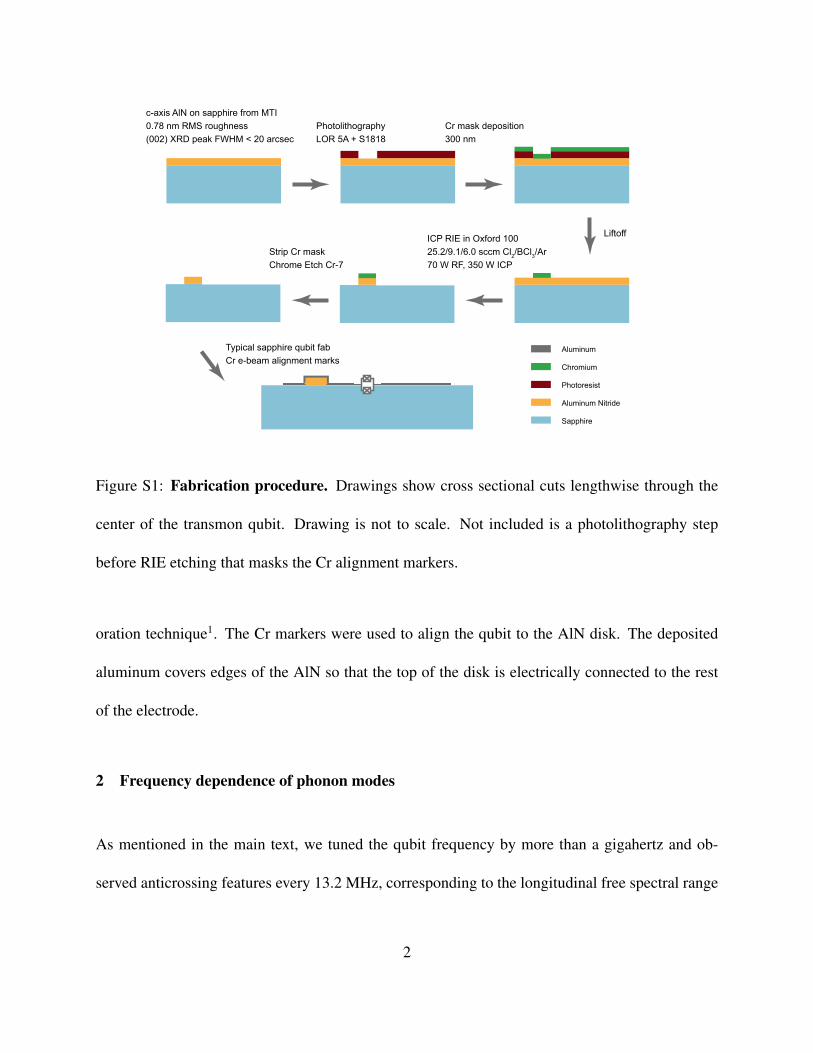
Figure S1: Fabrication procedure. Drawings show cross sectional cuts lengthwise through the

center of the transmon qubit. Drawing is not to scale. Not included is a photolithography step

before RIE etching that masks the Cr alignment markers.

oration technique1. The Cr markers were used to align the qubit to the AlN disk. The deposited

aluminum covers edges of the AlN so that the top of the disk is electrically connected to the rest

of the electrode.

2 Frequency dependence of phonon modes

As mentioned in the main text, we tuned the qubit frequency by more than a gigahertz and ob-

served anticrossing features every 13.2 MHz, corresponding to the longitudinal free spectral range

2

(FSR) of the phonon Fabry-Perot resonator. In Figure 2c and d of the main text, we presented spec-

troscopy and vacuum Rabi oscillations around the l = lmax − 2 = 503 longitudinal mode number.

In Figure S2a and c, we show results of the same experiments around l = lmax − 76 = 429. In

order to condense the information in Figure S2a, we take the maximum value in each horizontal

line and plot them in S2b. This maximum value plot highlights the substructure, including a dom-

inant anticrossing and a series of other features at higher frequencies. It is apparent in both the

spectroscopy and vacuum Rabi data that the substructure is qualitatively different from that of the

l = 503 data in Figure 2 of the main text.

We investigated nine different FSR’s to study this phenomenon. The frequency of the main

anticrossing feature, which corresponds to the deepest dip in the maximum value plots, is plotted in

S2d as function of FSR number. A linear fit gives a longitudinal phonon velocity of vl=1.11×104

m/s. In Figure S2e, we show the maximum value plots for each longitudinal mode number. Ac-

cording to Equation 2 in the main text, different values of l should only give rise to an overall

scaling of the relative frequencies of the transverse modes. We see, however, that the observed be-

havior is more complex, with the relative locations and intensities of the subfeatures changing with

l. This could be explained by the presence of the AlN, which provides some frequency-dependent

confinement for the phonons in the transverse directions.

3

! " #

$ %

!"#$%

&'("

)*l

Figure S2: Phonon modes at different frequencies. a, Spectroscopy around the l = 429 mode.

b, Maximum values from each horizontal line of a. From here on and in the text, we will call this

a maximum value plot. c, T1 and vacuum Rabi oscillations obtained using the same method as

Figure 2c in the main text. d, Frequency of the m = 0 transverse mode ωl,0 versus the longitudinal

mode number. The black line is a linear fit to the data. e, Maximum value plots for the longitudinal

modes shown in d after subtracting the frequency of them = 0 transverse mode for each. The plots

have been shifted vertically so that the background level for each curve approximately corresponds

to ωl,0 in gigahertz on the vertical axis.

4

3 Phonon T1 versus swap operation parameters

In Figure 4a of the main text, we presented phonon T1 data taken using an optimal swap pulse

between the phonon and qubit, whose length and amplitude are indicated by the white cross in

Figure 3a of the main text. However, since there is more than one phonon mode with different

transverse mode numbers, frequencies, and coupling strengths to the qubit, we investigated how

changing the swap pulse length and amplitude affects the measurement of phonon T1. The results

are presented in Figure S3. In Figure S3a and b, we see that, in addition to the slow oscillations

corresponding to the frequency difference between the m = 0 and m = 1 modes, there are fast

oscillations with a frequency of ∼ 3 MHz. This corresponds to the detuning between the qubit

during the swap pulse and when it is tuned away from the phonons during the delay. When the

swap pulse is imperfect, some population remains in the qubit during the delay period and evolves

at this detuning relative to the phonon. When the qubit is brought back into resonance with the

phonon for the second swap pulse, the populations interfere and give rise to the oscillations seen

in the data.

In Figure S3c, we show the effective T1 for each Stark pulse amplitude. We see that the T1

is maximum when the qubit population is most efficiently swapped into the phonon. Away from

these strongly coupled phonon modes, the T1 gradually reverts back to that of the uncoupled qubit.

The data in Figure S3 clearly shows that we are performing coherent operations between the qubit

and phonon, and that, in this case, the phonon can actually be used as a quantum memory that is

longer lived than the qubit.

5

a b

c

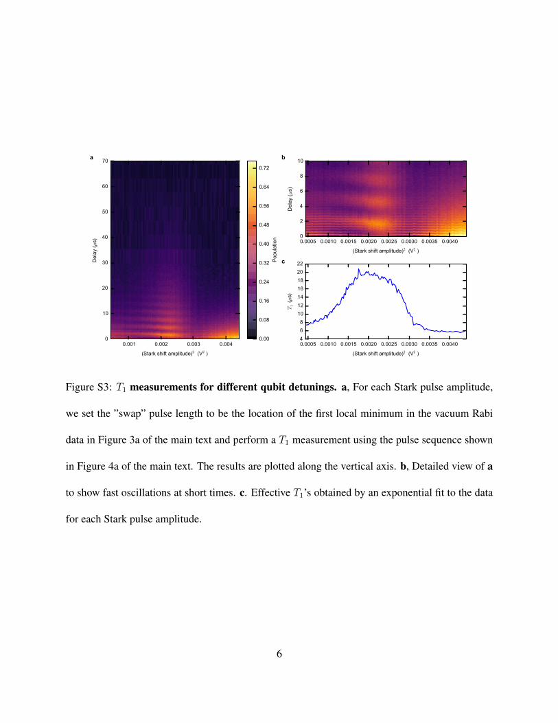
Figure S3: T1 measurements for different qubit detunings. a, For each Stark pulse amplitude,

we set the ”swap” pulse length to be the location of the first local minimum in the vacuum Rabi

data in Figure 3a of the main text and perform a T1 measurement using the pulse sequence shown

in Figure 4a of the main text. The results are plotted along the vertical axis. b, Detailed view of a

to show fast oscillations at short times. c. Effective T1’s obtained by an exponential fit to the data

for each Stark pulse amplitude.

6

4 Analysis of phonon modes

In the main text, we presented two complimentary ways to describe the mode structure and geo-

metric loss mechanisms of our system. Here, we explain these conceptual pictures in more detail

and give examples of how each can be used to analyze and understand different aspects of the sys-

tem. These descriptions are intended to give some physical intuition and qualitatively reproduce

the experimental results. We then present in the next section numerical simulations of a more exact

reproduction of the actual geometry.

Typically in cavity or circuit QED, we imagine an atom or superconducting qubit coupled

to a resonator, which is in turn coupled to the outside world through a partially reflecting mirror

or an evanescently coupled transmission line. We can describe the resonator as a photon box with

well-defined modes, and simplify the coupling to the modes of the surrounding environment into

a loss rate for each mode. There is, however, the opposite limit where the cavity is eliminated,

such as an antenna or an atom radiating into free space. In the case of the atom, for example, the

Wigner-Weisskopf theory of the spontaneous emission rate involves putting the atom in a large

fictitious box and considering its coupling to the semi-continuum modes of this box.

Physically, our system has features that resemble both a phonon box and a piezoelectric

transducer radiating into the “free space” of a bulk crystal. On the one hand, except for the 0.9 µm

disk of AlN protruding from one surface of the 420 µm thick substrate, there are no structures in

the transverse direction to confine the phonons. It is a phonon box with two ends but almost no

walls. The phonons are essentially free to propagate and diffract out of the box in the transverse

7

directions, which are semi-infinite due to the lossy boundaries of the sapphire. Therefore, as in the

case of the radiating atom, it seems reasonable to use the of modes of a semi-inifinite system to

calculate the diffraction loss of the phonons. On the other hand, if one considers the strain field

produced by the AlN transducer, one realizes that no transverse confinement is required to maintain

its energy for a long time inside the cylinder of substrate beneath the AlN. In other words, if we

consider this cylinder as our fictitious box, the strain field resembles a mode of this box with a

high quality factor. This is because the diameter of the AlN is ∼ 100 times larger than the phonon

wavelength. Therefore, the phonon mode undergoes very little diffraction as it propagates in the

longitudinal direction.

In order to model the phonon modes and their loss due to diffraction, we will use techniques

and concepts from both the lossy resonator and free space radiation pictures. We point out that, in

fact, any system with geometric or radiation loss can be simultaneously described in either picture,

depending on where one choses the boundaries of the system to be. In most cases, one of the

pictures is simply much more convenient for accurately modeling a particular aspect of the system

behavior.

Vacuum Rabi oscillations We first show two different ways of simulating the vacuum Rabi os-

cillations shown in Figure S2c and Figure 2c of the main text. The first method uses the modes

of a fictitious cylindrical box below the AlN, whose strain profiles are given in the main text and

reproduced here for convenience:

sl,m(~x) = βl,msin(lπz

h

)J0

(2j0,mr

d

). (S1)

8

J0 is the zeroth order Bessel function of the first kind and j0,m is the mth root of J0. h is the height

of the substrate and d is the diameter of the disk. βn,m is a normalization factor so that the total

energy of the mode equals ~ωq,m, where the mode frequency is given by

ωl,m =

√(lπ

h

)2

v2l +

(2j0,m

d

)2

v2t . (S2)

Here vl and vt are the longitudinal and effective transverse sound velocities, respectively. There-

fore, we have

βl,m =

√√√√√ ~ωl,m

πhc33

∫J0

(2j0,mr

d

)rdr

. (S3)

To find the coupling of these modes to the qubit, we can write the mechanical interaction en-

ergy as H = −∫σ(~x)s(~x) dV = −

∫c33d33(~x)E(~x)s(~x) dV . Here, σ(~x) is the stress, E(~x) is the

qubit’s electric field profile, and c33 and d33 are the stiffness and piezoelectric tensor components,

respectively. For simplicity, we are only considering the dominant tensor components perpendic-

ular to the surface of the substrate. Quantizing the qubit mode as E(~x)(a + a†) and the phonon

mode as s(~x)(b+ b†), we can use the rotating wave approximation to equate this interaction energy

to the Jaynes-Cummings Hamiltonian Hint = −~g(ab† + a†b). We then assume that the electric

field is a constant E0 throughout the transducer so that we maintain the cylindrical symmetry of

the problem. In reality, the electric field is slightly higher in the parts of the AlN that are closer to

the edges of the qubit electrode. In addition, by design, the thickness of the AlN is approximately

λa/2, where λa is the acoustic wavelength. Finally, making use of the fact that d33(~x) is a constant

d0 inside the AlN disk and zero elsewhere, we find

~gl,m = 2c33d0E0λaβl,m

∫ d/2

0

J0

(2j0,mr

d

)rdr (S4)

9

a b

0

1

2

0

1

2

Figure S4: Phonon modes and qubit coupling a, Qubit coupling strengths for the sl,m(~x) and

s′l,m(~x) modes for l = 503 as a function of mode frequency. Arrows and black crosses indicate

the modes plotted in b. For the sl,m(~x) modes, m = 0, 1, 2 are chosen. For the s′l,m(~x), we chose

m = 9, 33, 53, which correspond to the local extrema of the coupling strength. b. Comparison

of the radial parts of the phonon wavefunctions. By design, the sl,m(~x) modes go to zero at the

transverse boundary of the AlN disk, which has a radius of 100 µm. The s′l,m(~x), instead, go to

zero at r = 2 mm.

In Figure S4a, we show gl,m as a function of ωl,m for l = 503 and m from 0 to 3. Figure S4b

shows the m = 0, 1, 2 radial wavefunctions. The estimated value of g ∼ 2π × 300 kHz quoted in

the main text was obtained using the following constants in equations 2 and S4: vl = 1.11 × 104

m/s, vt = 8.78× 103 m/s, c33 = 390 GPa, d0 = 1 pm/V, and E0 = 2.9× 10−2 V/m. Note that the

value of vt is not simply the transverse sound velocity, but an effective value obtained by fitting

the acoustic dispersion surface2. The values of g shown in Figure S4a include an additional scale

factor to match the experimental data, as explained below.

We can now take gl,m and ωl,m as the qubit coupling strengths and frequencies of discrete

10

phonon modes and perform a full quantum mechanical simulation of vacuum Rabi oscillation

experiments. As in the experiment, the state is initialized with the qubit in the excited state and all

phonon modes in the vacuum state. It then evolves for a delay time according to the Hamiltonian

H = δqa†a+

∑m

δl,mb†l,mbl,m + gl,m(a†bl,m + ab†l,m), (S5)

where we are only summing over m and considering a single l since the longitudinal FSR is large

compared to the frequency range we’re interested in. a and bl,m are the annihilation operators for

the qubit and phonons, respectively. We have used the rotating frame at frequency ωl,0 so that δq and

δl,m are the detunings of the qubit and phonons from this frequency. We show the qubit population

at the end of this evolution in Figure S5a. The simulation were performed using the QuTip python

package3. To limit computation time, only the m = 0 to 3 modes were used. Along with the

experimentally measured qubit lifetime, phenomenological phonon lifetimes were introduced for

each phonon mode into the Lindblad master equation. We extract a coupling strength of gl,0 =

2π×260 kHz from our experimental data by applied an overall scaling to the coupling constants to

match the simulated results to the vacuum Rabi data. This is equivalent to multiplying the quantity

d0c33E0 by a factor of 0.85, which is justified since d0 and c33 are material constants have not been

independently measured for our materials at milikelvin temperatures, and E0 is an approximate

value taken from simulations. We see that the simulation results agree reasonably well with the

experimental data, indicating that the system can be modeled by a few discrete modes.

The introduction of phenomenological lifetimes for each phonon mode is necessary because

we chose a fictitious mode volume from which the energy is lost due to diffraction. Even though

the picture of discrete modes with loss rates seems to model the data quite well, energy loss due to

11

a b

Figure S5: Simulated Vacuum Rabi oscillations a, Results of full quantum simulation using the

sl,m(~x) modes for m = 0 to 3 and l = 503. The horizontal axis shows the qubit detuning from the

m = 0 phonon mode. b, Results of simulations using the s′l,m(~x) modes for l = 503, m = 0 to

80 and evolving the equations of motion for the mode amplitudes, as described in the text. White

cross indicates the frequency and duration of the swap operation used in calculations of phonon T1

and T2.

12

diffraction is not a Markovian process and we do not generally expect the time dynamics to follow

an exponential decay. For a more realistic model without any additional assumptions, we can

instead actually analyze the diffraction of phonons into a larger volume, say a cylinder with radius

a d. This can be done by finding the coupling of the qubit to the modes s′l,m(~x) of this large

cylinder, which have the same wavefunctions and frequencies as given in S4 and 2, except with d

replaced with a everywhere. In Figure S4a, we have plotted the coupling strength and frequencies

of the modes for a cylinder with a = 2 mm. We see that the s′l,m(~x) modes are much more

closely spaced in frequencies than the sq,m(~x) modes, as expected from the larger mode volume.

However, the shape of the transducer still determines the overall envelope of the coupling strengths

as a function of frequency, and we can identify local extrema that correspond to the sq,m(~x) modes.

To illustrate this correspondence, we have plotted the wavefunctions of the s′l,m(~x) at these extrema

in Figure S4b. We see that they resemble the wavefunctions of the sl,m(~x) modes.

In principle, we can now repeat the simulation of the vacuum Rabi oscillations in the same

way as for the sl,m(~x) modes. However, the more realistic picture comes at the cost of more

computational complexity. In the same frequency range, instead of four modes, we now have 80,

and full quantum mechanical calculation becomes impractical. However, if we start with the qubit

in the e state, the Hamiltonian in equation S5 only couples the initial state |1〉q|vac〉p to the states

|0〉q|l,m〉p, where the q subscript denotes the qubit and p denotes the phonon. |vac〉p denotes all

phonon modes in the vacuum state, and |l,m〉p denotes the s′l,m(~x) mode in the n = 1 Fock state

and all other modes in the vacuum state. Therefore, to reproduce the vacuum Rabi oscillations, we

13

can just solve the equations of motion for the amplitudes of these states:

cq(t) = (−γq + iδq)cq(t) +∑m

igl,mcl,m(t) (S6)

cl,m(t) = igl,mcq(t) + iδl,mcl,m(t) (S7)

Note that here, we have included the experimentally measured qubit decay rate, but the phonon

modes are lossless.

In Figure S5b, we plot |cq|2 as a function of interaction time for various δq with l = 503. We

see that it also approximately produces the main features of the vacuum Rabi data. Unlike Figure

S5a, these simulation results do not assume discrete phonon modes with phenomenological decay

rates. They show that the behavior of our system is well described by a first principles model of

phonon propagation and diffraction in a semi-infinite system.

The calculations above are valid for a resonator with two completely flat mirrors. In real-

ity, the AlN disk protrudes above the surface and provides some confinement for the phonons.

Therefore, our physical system is likely to be in an intermediate regime between the two models

described above, as evidenced by the qualitative change in the phonon spectrum as a function of

longitudinal mode number. Neither model completely captures the details the system dynamics,

and the more subtle characteristics need to be simulated using more sophisticated methods, es-

pecially if we want to use more complicated geometries such as curved surfaces to confine the

phonons and simplify the mode structure. We will demonstrate such a method in section 5. First,

however, we show how the semi-continuum model can be used to estimate the lifetime of phonons.

14

Phonon lifetime In this section, we present a way of estimating the diffraction limited lifetime

of the phonons, as measured in the T1 experiment presented in Figure 4a of the main text. In this

experiment, we initialize the phonons in some state s(~x, τ = 0) after a swap operation. In our

calculations, we decompose s(~x, τ = 0) into the s′l,m(~x) basis, with amplitudes cl,m obtained by

integrating the equation S7 for a time tswap. Just as in the experiment, we chose a qubit frequency

and tswap, indicated by a white cross in Figure S5b, which most efficiently transfers the qubit state

to the phonons. Since the s′l,m(~x) are eigenmodes of the system, we can simply calculate the state

of the phonons after diffracting for a time τ as

s(~x, τ) = cl,me−iωl,mτs′l,m(~x). (S8)

In the experiment, doing the second swap operation and measuring the state of the qubit corre-

sponds to measuring the overlap of the phonon state s(~x, τ) with the original state s(~x, τ = 0),

which we will call η(τ). Specifically, the measured signal is proportional to

|〈s(~x, τ = 0)|s(~x, τ)〉|2 = |η(τ)|2 (S9)

=

∣∣∣∣∣∑m

|cl,m|2 eiωl,mτ

∣∣∣∣∣2

(S10)

Similarly, one can find that the measured T2 signal has the form(1 +Re

[eiΩτη(τ)

])/2.

We plot the simulated T1 and T2 results in Figure S6. We see that the simulation qualitatively

reproduces the features of the data in Figure 4 of the main text, with a few deviations. First, we

see the effects of the finite mode volume at long times, when the simulated wavefunction starts to

reflect back from the boundaries. Second, the timescales are a few microseconds, which is on the

same order as but somewhat shorter than the experimentally measured values. This could be due

15

0 10 20 30 40 50Delay (µs)

0.0

0.1

0.2

0.3

0.4

0.5

0.6

0.7

0.8

0.9

Pop

ulat

ion

T1

T2

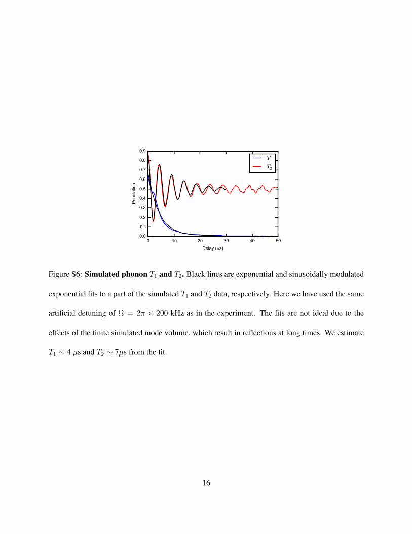
Figure S6: Simulated phonon T1 and T2. Black lines are exponential and sinusoidally modulated

exponential fits to a part of the simulated T1 and T2 data, respectively. Here we have used the same

artificial detuning of Ω = 2π × 200 kHz as in the experiment. The fits are not ideal due to the

effects of the finite simulated mode volume, which result in reflections at long times. We estimate

T1 ∼ 4 µs and T2 ∼ 7µs from the fit.

16

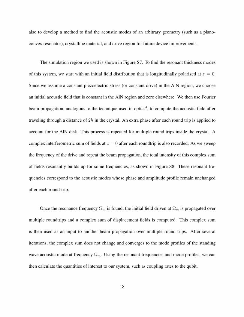
Absorbing layer 900 nm thick AlN

Sapphire 420 um

200um

1 mm

z=0

z=h

Figure S7: Simulation geometry including the AlN disk. We consider a cylindrical sapphire

substrate with two flat faces. The diameter of the cylindrical region is 1 mm and the height is 420

µm. An AlN disk of thickness 900 nm and diameter 200 µm protrudes from the center of one face.

An absorbing layer is added to mitigate unwanted reflection from the transverse boundaries and

simulate lossy boundaries of the sapphire. We use 11110 m/s and 6056 m/s as the longitudinal and

transverse velocities for sapphire, respectively. We use 11008 m/s for the longitudinal velocity of

sound in AlN.

to the confinement of the modes by the AlN in the physical system, which is not included in the

simulation. Finally, the initial populations in the simulated data are higher because qubit decay

during the second swap pulse is not included.

5 Beam propagation simulations: Finding acoustic modes with AlN

In this section, we use acoustic beam propagation and the method of resonant acoustic excitation to

determine acoustic modes of our system with the effects of AlN disk included2. We were motivated

to develop this simulation technique not just to understand any additional effects of the AlN, but

17

also to develop a method to find the acoustic modes of an arbitrary geometry (such as a plano-

convex resonator), crystalline material, and drive region for future device improvements.

The simulation region we used is shown in Figure S7. To find the resonant thickness modes

of this system, we start with an initial field distribution that is longitudinally polarized at z = 0.

Since we assume a constant piezoelectric stress (or constant drive) in the AlN region, we choose

an initial acoustic field that is constant in the AlN region and zero elsewhere. We then use Fourier

beam propagation, analogous to the technique used in optics4, to compute the acoustic field after

traveling through a distance of 2h in the crystal. An extra phase after each round trip is applied to

account for the AlN disk. This process is repeated for multiple round trips inside the crystal. A

complex interferometric sum of fields at z = 0 after each roundtrip is also recorded. As we sweep

the frequency of the drive and repeat the beam propagation, the total intensity of this complex sum

of fields resonantly builds up for some frequencies, as shown in Figure S8. These resonant fre-

quencies correspond to the acoustic modes whose phase and amplitude profile remain unchanged

after each round-trip.

Once the resonance frequency Ωm is found, the initial field driven at Ωm is propagated over

multiple roundtrips and a complex sum of displacement fields is computed. This complex sum

is then used as an input to another beam propagation over multiple round trips. After several

iterations, the complex sum does not change and converges to the mode profiles of the standing

wave acoustic mode at frequency Ωm. Using the resonant frequencies and mode profiles, we can

then calculate the quantities of interest to our system, such as coupling rates to the qubit.

18

6 7 8 90

20

40

60

80

Ampl

itude

(a.u

.)

l = 429l = 503

6 7 8 90

5

10

15

20

log

of In

tens

ity (a

.u.)

Measurement

Simulation

0 100-100-100

100

0

x(um)

y(um

)

0 100-100-100

100

0

x(um)

y(um

)

i)

ii)iii)

i) ii)

0

1

0 100-100-100

100

0

x(um)

y(um

)

iii)

a

b

c

Figure S8: Resonant frequencies and mode profiles including the effect of AlN. a. Maximum

value plot taken from the spectroscopy data for modes around l = 429 and l = 503. The amplitude

axis is inverted for ease of comparison with simulation results. b. Total acoustic intensity integrated

over the z= 0 plane showing the resonant frequencies from the beam propagation simulation for

l = 429 and l = 503 modes. c. Acoustic intensity profiles of the resonant acoustic modes around

l = 503. These mode profiles are cross-sections of the 3D acoustic modes taken at z = 0.

19

We compare the features in the maximum value plot obtained from the spectroscopy data

(See Figure S2) around the l = 429 and l = 503 modes with the resonant frequencies from

the simulation in Figure S8. Since the absolute frequencies of simulated modes depend on the

longitudinal sound velocity, which is not precisely known, we have lined up the m = 0 modes in

the maximum value plot for both l = 429 and l = 503 modes with their respective frequency values

from the simulation. This allows us to compare the relative spacings of the higher order transverse

modes. The dotted lines between Figure S8b and S8c suggests that the relative spacing between

the higher order modes in the simulation matches reasonably well with the measurement. The

simulations indicate that at lower longitudinal mode number l (corresponding to smaller phonon

frequencies), the separation between the higher order transverse modes increases as observed in

the experiment. It can be observed from the data that the ratios of separations also change, and this

is qualitatively reproduced by the simulations. We point out that the the maximum value plots are

not a direct measurement of the total field intensity of the acoustic modes and depends on more

complex aspects of the system such as the coupling to the qubit. Discrepancies between the data

and simulation can be attributed to this, along with other factors such as non-uniformities in the

electric field and uncertainties in the AlN thickness. Therefore we simply aim to compare the

frequency spacings of the modes and verify that our understanding of the experimentally observed

mode structure is valid with the inclusion of the AlN.

Once the resonant mode frequencies are found, we computed acoustic intensity profiles for

modes around l = 503 at z = 0 (See Figure S8 c)). These acoustic mode intensity plots show

that most of the acoustic energy for these modes is confined within the AlN region. These modes

20

nonetheless extend all throughout the simulation domain and suffer absorption losses at the simula-

tion boundaries. The leaky nature of these modes is also evident in the finite width of the resonant

spectrum in our simulation.

For future device improvements, we will use these simulation techniques to design resonators

with shaped boundaries, such as a plano-convex geometry. This should allow for lateral confine-

ment of thickness acoustic modes and result in a dramatic increase in phonon coherences. Addi-

tionally, these simulations will help us identify the correct shape for the AlN drive region so that

we can tailor the coupling to a single phonon mode.

1. Wang, C. et al. Surface participation and dielectric loss in superconducting qubits. Applied

Physics Letters 107, 162601 (2015).

2. Renninger, W. H., Kharel, P., Behunin, R. O. & Rakich, P. T. Bulk crystalline optomechanics

(in preparation).

3. Johansson, J., Nation, P. & Nori, F. Qutip: An open-source python framework for the dynamics

of open quantum systems. Computer Physics Communications 183, 1760 – 1772 (2012).

4. Fox, A. & Li, T. Computation of optical resonator modes by the method of resonance excitation.

IEEE Journal of Quantum Electronics 4, 460–465 (1968).

21