Quantitative Trading System

Denis Andrey Ignatovichdenis.ignatovich@mccombs.utexas.edu

May 5, 2006

Abstract

My interests are in the study of market microstructures, that is, howtrading takes place in the markets and how those markets are organized.Models are designed to describe aspects of these organizations and oneneeds flexible toolsets for model description and performance analysis.The current step in my research is an implementation of a quantitativetrading system. Not only is this a challenging systems engineering project,but also a powerful mechanism for data analysis and trade algorithmdescription.

Trading Model is defined as an investment tool comprised of buy andsell recommendations. These recommendations are much more complexthan simple price change forecasts. They must be taylored to the investorin terms of his/her risk exposure, past trading history, and the marketmicrostructure with its own constraints on the trade execution. A tradingmodel has three main components:

• Generation of the trading recommendations.

• Accounting of the simulated transactions and their price impacts.

• Generation of the model statistics by the performance calculator.

A Trading System is, in turn, an environment where users define and,through execution feedback, adjust their trading models. An essentialpart of the system is the user-interface: it must be eloquent enough toallow an ease-of-use and, at the same time, powerful to describe mostsophisticated trading algorithms. As in forecasting or other applications,trading models rely heavily on the quality of financial data. This con-straint on the Trading System, a supply of the tick-by-tick data, is just anexample of the multitude of requirements of a functional real-time tradingenvironment.

Thie following paper describes an implementation of a quantiativetrading system designed to incorporate features representative of a com-mercial grade trading environment. The system that I propose includesprogrammatic access to the underlying execution framework, powerfulPython-based algorithm description environment, real-time data support,and mathetmatical interfaces, including support for ARCH-based equityvolatility models.

This paper, in part, fulfills the degree requirement for Bachelor ofScience in Computer Sciences (Turing Scholars Option).

1

Contents

1 Introduction 2

2 System Model 3

3 System Architecture 43.1 Overview . . . . . . . . . . . . . . . . . . . . . . . . . . . . . . . 43.2 QuantWorld . . . . . . . . . . . . . . . . . . . . . . . . . . . . . . 53.3 Interface . . . . . . . . . . . . . . . . . . . . . . . . . . . . . . . . 53.4 Trading Model . . . . . . . . . . . . . . . . . . . . . . . . . . . . 83.5 Matrix . . . . . . . . . . . . . . . . . . . . . . . . . . . . . . . . . 93.6 ControlCenter . . . . . . . . . . . . . . . . . . . . . . . . . . . . . 103.7 Data Server . . . . . . . . . . . . . . . . . . . . . . . . . . . . . . 10

3.7.1 Functionality . . . . . . . . . . . . . . . . . . . . . . . . . 103.7.2 Database Schema . . . . . . . . . . . . . . . . . . . . . . . 11

3.8 Implementation . . . . . . . . . . . . . . . . . . . . . . . . . . . . 11

4 Application 114.1 Introduction . . . . . . . . . . . . . . . . . . . . . . . . . . . . . . 114.2 Optimal Risky Portfolios . . . . . . . . . . . . . . . . . . . . . . . 134.3 CMT & CAPM . . . . . . . . . . . . . . . . . . . . . . . . . . . . 144.4 Index Models . . . . . . . . . . . . . . . . . . . . . . . . . . . . . 164.5 Data Filtering and VWAP Calculation . . . . . . . . . . . . . . . 174.6 GARCH-based Volatility Calculation . . . . . . . . . . . . . . . . 174.7 Complete Algorithm . . . . . . . . . . . . . . . . . . . . . . . . . 18

5 Future Work 19

6 Acknowledgements 19

References 19

1 Introduction

Quant is an algorithmic trading system. Using Python, users define dataanalysis and trading algorithms. The destinction is that former operate on in-homogeneous time series (tick data) and publish results to trading algorithms,that make trade decisions for portfolios they are responsible for. Users createportfolios by specifying their descriptions and initial capital. A portfolio may bemanaged by the PortfolioManager (part of TradingModel, please see below) thatsimply updates portfolio positions with the user manually modifying their com-position weights. Alternatively, the user will assign a custom trading algorithmthat would make the decisions automatically upon receiving signals of new dataarrival. R-statistical environment provides the many necessary computationaltools for making informed decisions.

2

2 System Model

QuantWorld ’s synthetic trades Designing solution to an engineering prob-lem must start with analyzing the requirements in terms of input data, preci-sion/algorithm running complexity, and results’ presentation. In the case ofQuant, there is an important issue of quality data: real-world trading systemsrely on fast and precise trade information (and recently with the introductionof NYSE’s OpenBook, even the specialists’ books) for decision making. Lack ofaccess to this level of data forces numerous assumptions on the part of the traderdesigning the algorithms. Yahoo! Finance provides 20-minute delayed price in-formation distributed once per minute. It is the most commonly used source offinancial data outside of the commercial realm, and due to the economic con-straints of this project, it will service us with the foundation of our trade data.The necessary environment for the trade algorithm execution must provide themost up-to-date price information. The transition from Yahoo! Finance datato our algorithm environment (TradingModel) is supplied by QuantWorld, acomponent outside the trading system that simulates high-frequency data gen-eration. The simulation will result in synthetic ticks containing bid/ask, price,and volume information distributed according to the parameters set by the user.The necessity of this price generation is specific to the author’s use of the sys-tem, and therefore QuantWorld ’s residence outside of the system allows for ansubstitution of a pricing information feed accomodating purposes of anotheruser.

Data vs. Trading Algorithms Many operations performed by the users’algorithms would be quiet common data handling tasks. Thus, the decision toprovide two algorithmic interfaces was raised by the need to factor out redundanttasks. The Matrix runs data-analysis algorithms and publishes the results forthe trading algorithms.

UserInterface The UserInterface handles the task of informing the trader ofnot only the status and performance of his/her trading algorithms, but also pro-vides a flexible means of their manipulation and adjustment. From my personalexperiences in the industry, I have learned the ingenuity of Microsoft Excel ’sinterface. Many plug-ins to Excel form the foundation for decision making onWall Street, and in my opinion, a successful system would incorporate theseparadigms. At the same time, there are many tasks requiring programmaticaccessibility. For this purpose, I have adopted PyCute’s model of a QT built-incommand line parser for the interface. The control mechanism provided withthe command line (or shell) entails priority execution mechanism such that anyof the user commands vital to the system are executed before any data manip-ulation.

Summary The following are the main abstract goals of the system that servedme as guides for the implementation:

interchangable data feed

real-time execution

flexible algorithm environment

3

3 System Architecture

3.1 Overview

Considering the constraints of a real-time system, components working onindependant tasks must operate as individual threads. With this decision inmind, the next question was the method of facilitating communication betweenthem. The most simple solution was to provide each component with a mes-saging queue and provide all other components with a reference to that queue.Whenit produced stock data, for example, the Matrix would create a threadthat would wait for a notification of release of Trading Model ’s queue and theninsert the data. During the next iteration in the execution loop, Trading Modelwould wait on its queue and process the data. With the numerous referencesand deadlocks, I began to look for a different solution. After discussing the issuewith Dr. Lavender, he recommended a publisher/subscriber model. I researchedseveral implementations for Python and stopped on Netsvc for several reasons:for the most part, it is written in Python (no overhead code or installationsneeded with future deployment) and it has a very clean interface, yet enough tocover my requirements.

Netsvc package is used in two dimensions: (1) HTTP Daemon serves RemoteProcedure Calls between the User Interface and the ControlCenter, and (2)Message Dispatcher runs the Publisher/Subscriber model internal to the system.The components communicate via several channels separated on the type ofcommunication: data, messages, and commands. All messages sent within thesystem are of the following format:

(source, commType, args)

where:

source - string identifying component sending the message

commType - string indicating communication type (‘message’, ‘data’, or ‘com-mand’)

args - tuple to be further parsed by the receiver

Messages are published through instantiating an object of the class Netsvc.Serviceand calling its method, publish with the message content and the intended chan-nel. Components receive messages from a particular channel by, similarly, in-stantiating an object of the class Netsvc.Service and specifying the channels forsubscription and callback methods for message handling. The callback methodsinsert messages onto a thread-safe queue that the component polls in its threadloop.

Component Descriptions:

Broker - receives trade requests and simulates the ’price impact’ function.That is, user does not necessarily receive stocks at the price they arelisted. Trading algorithms must account for this. Parameters of the impactsimulator are set by the admin, similarly to the QuantWorld settings.

4

ControlCenter - the main component. It is responsible for starting/maintainingthe other modules and servicing user requests submitted via RPC. It alsoaggregates data for the GUI output: stock data, system messages, requestsresults, and debug information.

TradingModel - creates/loads/runs user trading algorithms. When an algo-rithm makes a trade request, the model checks the parameters againstcurrent positions (do not sell more than currently have, unless short posi-tions are allowed).

Matrix - ‘listens’ for the trade data submitted by QuantWorld, processes it,and performs additional user-specified operations, and then publishes re-sults onto the network. The goal was to factor out common data opera-tions used by several algorithms.

DataServer - stores trade data and any modifications to the current systemstate (new users, new algorithms, etc.)

Both the UI and QuantWorld were developed using QT’s Designer. It is agreat tool for constructing user interfaces that uses a middle language to describeforms in an implementation-independent way. After the Designer produces anXML description of the application, it is translated into Python class usingpyuic that is used to derive GUI applications. An issue came up with signalinterrupts for network communication while using QT’s main event loop andsignal handling methods. QT’s messaging mechanism was incompatible withother signal handling utilities, uncluding the Netsvc package. The bypass wasto simply rely on the Http RPC methodology. Trolltech is scheduled to releasea flexible interface for custom signal handlers in the upcoming QT version.However, due to the open source nature of the Python implementation of Qt,it is unlikely this feature would be available for Python users any time soon.

3.2 QuantWorld

QuantWorld provides the necessity of a trading system: access to real-timedata (synthetic). The user inserts companies he/she wishes to simulate, Quant-World then queries Yahoo! Finance for their information. Every two minutes,QuantWorld polls the latest price for every company in the list. Between theupdate-periods, a Monte Carlo simulation ‘produces’ trades based on the latestprice. The user can adjust both trade generation frequency and volatility. Thetrades are published onto the network for the Matrix to process. The frequencyranges from 1 to 120, or at maximum twice a second. A schedule is created ev-ery two minutes for each individual security in the list: based on the frequency,the times when a company will trade are randomly picked and marked in theschedule. For the next two minutes, the timer signal will call on a routine everyhalf second and would compare the current time against stocks’ schedules, andgenerate trades in cases of a match.

3.3 Interface

The User Interface connects to the system via HTTP, thus user can loginfrom any place in the world with an Internet connection. There are three main

5

Figure 1: Quant System Architecture6

Figure 2: QuantWorld v1.0

components: command shell, messaging window, and the display. Derived fromPython’s Cmd Class, command shell provides programmatic access to the sys-tem. Initially, only the login command is visible to the user. He/she may type‘help’ to view the full list of commands available. By typing ‘help’ followed byname of the comman, usage examples and detailed information are printed out.When the user enters a command, it is first parsed and checked for correct for-matting, and then sent to the system (through a central point in the interface)along with additional user information. After successfully logging in (request isverified with the database), user’s Workspace is initialized containing the stockshe/she is following on the display and the algorithms with respective portfo-lios loaded. Any changes to the Workspace are stored within the system, thusshould the connection fail, data will be recovered.

Messaging screen echoes messages within the system (debugging informa-tion, if the option is selected, and system warning messages) and prints resultsof commands that user submitted. UI has an internal timer that executes ev-ery half of a second. On the timer event, UI asks the ControlCenter for thelatest messages and resets the messaging queue in the system. For example,these include results of all portfolios’ listing (with their descriptions, algorithmsrunning it, current positions, etc.), the output will appear in the messagingwindow. System warnings and debug stream (if this option is set) are routedhere as well.

The display is split into three pages: the matrix, stock visualization, andstrategies’ screen. The Matrix is an Excel spread-sheet like form with continu-ously updated company information (latest price, moving average, transactionvolume, etc.), as well as results of any custom data analysis algorithms. The

7

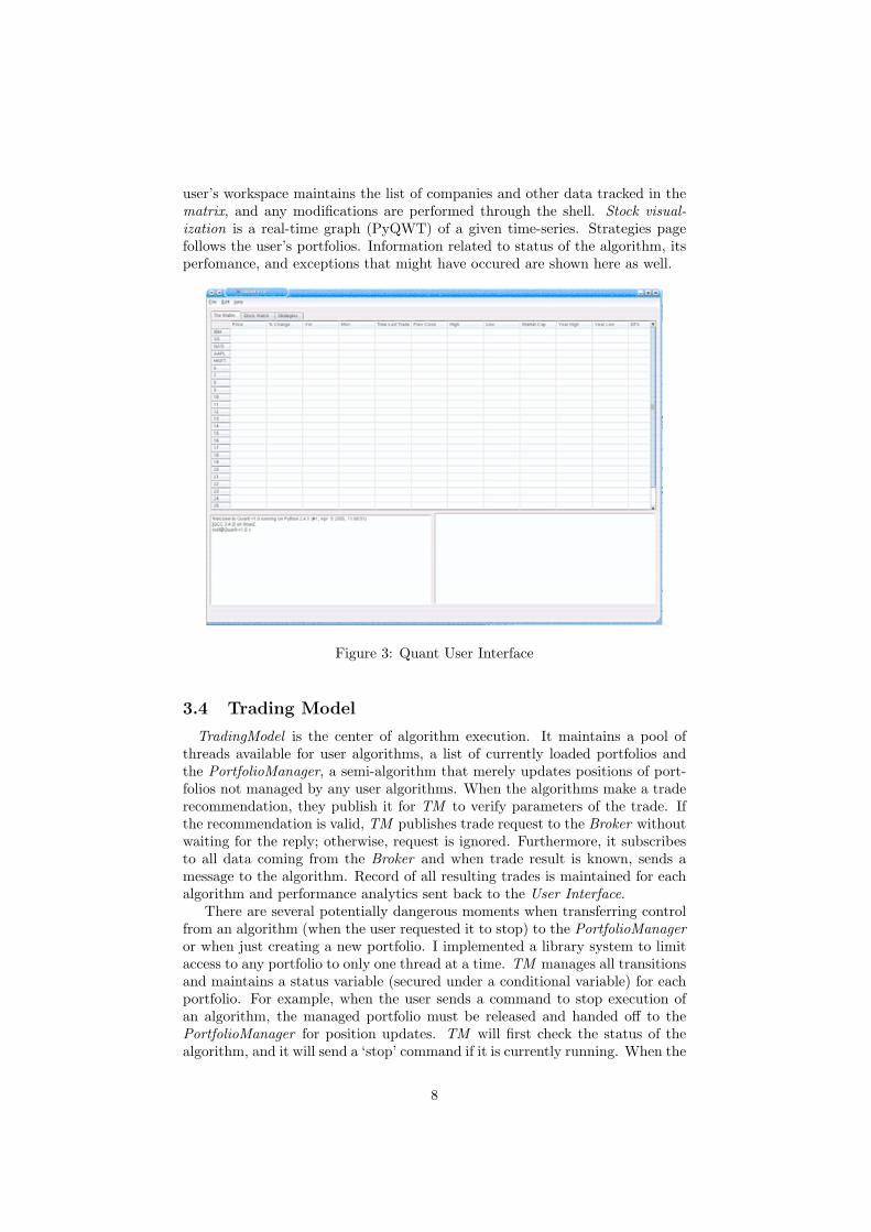
user’s workspace maintains the list of companies and other data tracked in thematrix, and any modifications are performed through the shell. Stock visual-ization is a real-time graph (PyQWT) of a given time-series. Strategies pagefollows the user’s portfolios. Information related to status of the algorithm, itsperfomance, and exceptions that might have occured are shown here as well.

Figure 3: Quant User Interface

3.4 Trading Model

TradingModel is the center of algorithm execution. It maintains a pool ofthreads available for user algorithms, a list of currently loaded portfolios andthe PortfolioManager, a semi-algorithm that merely updates positions of port-folios not managed by any user algorithms. When the algorithms make a traderecommendation, they publish it for TM to verify parameters of the trade. Ifthe recommendation is valid, TM publishes trade request to the Broker withoutwaiting for the reply; otherwise, request is ignored. Furthermore, it subscribesto all data coming from the Broker and when trade result is known, sends amessage to the algorithm. Record of all resulting trades is maintained for eachalgorithm and performance analytics sent back to the User Interface.

There are several potentially dangerous moments when transferring controlfrom an algorithm (when the user requested it to stop) to the PortfolioManageror when just creating a new portfolio. I implemented a library system to limitaccess to any portfolio to only one thread at a time. TM manages all transitionsand maintains a status variable (secured under a conditional variable) for eachportfolio. For example, when the user sends a command to stop execution ofan algorithm, the managed portfolio must be released and handed off to thePortfolioManager for position updates. TM will first check the status of thealgorithm, and it will send a ‘stop’ command if it is currently running. When the

8

algorithm parses that command, it will cease all operations and send a requestof transfer back to the TM. After processing the transfer request, the portfoliowill be added into the PortfolioManager ’s influence.

Figure 4: Trading Model UML

3.5 Matrix

As stated above, the Matrix processes trade data published by the Quant-World. Its structure is similar to the TradingModel : a listener object subscribesto the data feed and inserts trades onto the queue. The Matrix Thread thendistributes trade data among the data analysis algorithms that, in turn, processit and publish their results via ‘data’ channel. The format for submission is adictionary that contains two fields, ‘ticker’ and ‘type’, and an arbitrary numberof data values. As there are no shared objects, the implementation is fairlystraight forward. The interface for inserting/removing algorithms is similarto TM ’s. Specifically, commands are published with destination ‘Matrix’ thatspecify the Python code for the algorithm and the owner’s userId. A new thread

9

is created with access to the incoming data and the algorithm information isbacked into the database.

Figure 5: Matrix UML

3.6 ControlCenter

ControlCenter is the only component that is not derived from a thread. Itspurpose is to provide access to the system and maintain ‘sanity’ of the com-ponents. After it starts up the exchange server, messaging dispatcher, andthreads running the components, it communicates with them only via pub-lisher/subscriber architecture. On the side of UserInterface, it creates an Http-Daemon and exports several methods via RPC:

command (user, func, args) - central method that matches request with anoperation and dispatches command to the component

checkConnection (user) - returns status of the user within the system

setupWorkspace - initializes user’s workspace: loads the list of stocks trackedthrough UI, loads portfolios and algorithms

retrieveMessages - returns internal system messages and resets the messagingqueue

retrieveShellMessages - returns messages labeled for shell output (resultsfrom user requests to components) and also clears the queue

retrieveStockData - returns latest stock information as specified by the workspace

retrievePortData - returns user’s portfolio and algorithm information

3.7 Data Server

3.7.1 Functionality

The DataServer stores all changes to the system state into MySQL server.This includes all communication except system and shell messages. Since the

10

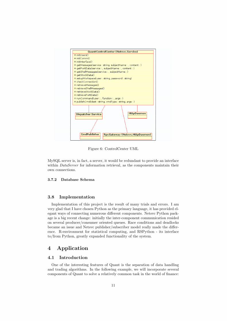
Figure 6: ControlCenter UML

MySQL server is, in fact, a server, it would be redundant to provide an interfacewithin DataServer for information retrieval, as the components maintain theirown connections.

3.7.2 Database Schema

3.8 Implementation

Implementation of this project is the result of many trials and errors. I amvery glad that I have chosen Python as the primary language, it has provided el-egant ways of connecting numerous different components. Netsvc Python pack-age is a big recent change: initially the inter-component communication residedon several producer/consumer oriented queues. Race conditions and deadlocksbecame an issue and Netsvc publisher/subscriber model really made the differ-ence. R-environment for statistical computing, and RSPython - its interfaceto/from Python, greatly expanded functionality of the system.

4 Application

4.1 Introduction

One of the interesting features of Quant is the separation of data handlingand trading algorithms. In the following example, we will incorporate severalcomponents of Quant to solve a relatively common task in the world of finance:

11

Figure 7: SQL Schema

12

portfolio optimization. Two data sources are available to us: (1) the historicalprices (courtesy of Yahoo! Finance) for volatility calculation, and (2) real-timetrade data supplied by QuantWorld for the current returns and correlations.Since we’re given heterogeneous (inhomongeneous) time series, i.e. irregularlyspaced, we will compute volume-weighted average price (VWAP) for normal-ization of each series (this will provide us with a common point of reference forall of the stocks in the portfolio). The next step would be to take the histor-ical prices and run Generalized Autoregressive Conditional Heteroskedasticity(GARCH) model to compute conditional variance (risk) for the series. Once wehave both of these results, we will run quadratic optimization to determine thebest weights’ allocation for our portfolio.

4.2 Optimal Risky Portfolios

Our goal is to efficiently construct a diversified portfolio of equity securities.By efficiently, we mean deriving the most out of the risk we infer from makingour investments. There are two sources of risk to our portfolio: market (orsystematic) and firm-specific. Every security has exposure to systematic risk, itis inherent to all stocks traded in the market. The effect of diversification, how-ever, is derived from combining securities whose firm-specific risks offset eachother. For example, when oil futures’ prices rise, an oil company’s stock pricewill rise, while high-tech’s may fall. This effect is the foundation of diversifica-tion and in the next several sections we will look at tools allowing us to describecomposition of portfolios such that we minimize the non-systematic risk and at-tain highest-possible return per unit of risk. The concept of diversification waspresented by Harry Markowitz in his “Portfolio Selection” article in Journal ofFinance, 1952 [15] as part of his Modern Portfolio Theory.

The model started out by making numerous unrealistic assumptions:[3]

1. Potential investments are derived from a probability distribution of ex-pected returns.

2. Wealth has a diminishing marginal utility.

3. Decisions are made based on expected return and risk.

4. Risk is a function of variance of past returns.

5. Investors are rational: from a set of investments at the same risk level,they will prefer one with the highest return.

We will now proceed by examining the basic units we will use to furtherdevelop our models. Average of the underlying stocks’ returns measures returnof the overall portfolio.

rp = w1r1 + w2r2

Non-linearity of the portfolio’s risk (as shown below for a two-asset portfolio)will provide us with the key for diversification:

σ2p = w2

1σ21 + w2

2σ22 + 2w1w2Cov(r1, r2)

13

The last term in the equation will be negative for stocks that historicallyoffset each other’s risks, that is, to some extend, they move in opposite direc-tions. Therefore, overall portfolio risk will be less than just the weighted averageof the two. The effect of their combination is illustrated in Figure: Effects ofDiversification, where there are several portfolio opportunity sets for differentlevels of correlation. In theoretical finance, the more risk an investment entails,the higher return the investor will seek and vice versa. The ratio of return torisk varies with different assets; that taken together will provide us with ratiofor our portfolio. Our goal is to derive weights, or fractions of overall capitalinvested in individual assets, such that we derive the most return per unit ofrisk. US Government Treasury Bills, or T-bills, are considered risk-free assets,and they symbolize the minimum absolute return an investor should seek. Wewill come back to this concept when we discuss CAPM, a model that addressedcombination of the risk-free asset and MPT’s efficient portfolio.

Efficient frontier is a set of portfolios, such that, for any risk level, theportfolio with the highest return is included in this set. “Alternatively, thefrontier is the set of portfolios that minimize the variance for any target expectedreturn” [4]. Given our set of securities, MPT suggests forming a portfolio thatwould lie on the efficient frontier.

One of the limitations of MPT is the reliance on expectation of securities’returns. The issue is the assumption of efficient markets. We do not have anyinformation that is not already available to the general public. Thus, only thehistorical data is available to us, but we must form expectations of the futurereturns.

Figure 8: Effects of diversification in a simple two-asset portfolio

4.3 CMT & CAPM

Capital Markets Theory was introduced by William Sharpe (Jack Treynor,John Litner, and Jan Mossin also arrived at the theory independently) in 1964and was based on Markowitz’s MPT of twelve years earlier. The model startsout with the same set of assumptions as MPT and adds severl others [3]:

1. Investors form their portfolios on the MPT’s efficient frontier.

14

Figure 9: Forming an efficient frontier

2. As noted above, there is an asset with zero risk (T-Bill), and investorsmay borrow and lend at its rate.

3. Investors have homogeneous expectations of future returns.

4. All investors share the same investment horizon.

5. The operating microstructure has no transaction costs.

6. The interest rates (that dictate, among other things, the risk-free rate)are constant.

7. All investments are properly priced (no arbitrage opportunities).

As stated above, MPT dictates that the only portfolios we would like toform are on the efficient frontier. But how would one account for the risk-freeasset that is visualized on the return (vertical) axis? As it turns out, if we thinkabout how portfolio variance and return are computed and combine our efficientportfolio with a risk-free asset, a new efficient frontier will form. Let i denoteour portfolio on the efficient frontier. If we combine it with a risk-free asset, thereturn will equal:

E(Rport) = wRF (RFR) + (1− wRF )E(Ri),and σ2

port = w2RF σ2

RF + 2wRF (1− wRF )rRFiσRF σi.

But, by definition, risk-free rate has zero variance and its covariance withany asset would be zero, we therefore derive the following definition:

σport = (1− wRF )(2)σ2i

This linear relationship provides us with means of stepping out of our ef-ficient frontier by shifting capital in/out of our efficient portfolio and invest-ing/leveragin the risk-free asset. We still have to keep in mind the return-to-riskratio. When we look at all of the possible lines or opportunities of combiningefficient portfolios with the risk-free asset, we will notice that there is one that

15

will dominate all others in terms of that ratio. This line is referred to as Cap-ital Market Line (CML) and is formed by two points: the risk-free rate andthe tangency portfolio on the efficient frontier. The latter is called the MarketPortfolio and since the markets are in equilibrium, it combines all assets in theworld (including those not traded).

If we wish to increase the return of our overall portfolio, we simply borrowat the risk-free rate and reinvest the proceeds into the Market Portfolio. Theresult will dominate the portfolio on the efficient frontier. Even though thisnotion of a portfolio combined of all assets in the world, and that is furthercomplicated by the assumption of markets in equilibrium, we will later use it toderive a model we can easily implement.

Capital Asset Pricing Model (CAPM) understands that every asset shouldbe as close to the CML as possible. And derives the source of risk of an assetas its measure of variances with the Market Portfolio, β.

E(ri = rf + βi[E(rM − rf ]where: β = Cov(ri, rM )/σ2

M

Beta can be viewed as a systematic measure of risk[3]. Since covariance of anasset with itself is just the variance, β of the Market Portfolio is 1. Assets withβ above 1 are considered more volatile than the market and vice versa. Thislinear relationship forms the Security Market Line and it provides a measureof the market-required rate of return. An analyst may compare this expectedreturn against his own expectations to determine whether the asset is pricedcorrectly. The importance of CAPM to our cause is the relationship betweenrisk and expected return of a security, and in the next section we will tie in pastreturns to arrive at a solution to our goal of portfolio optimization.

4.4 Index Models

Risk is probability that investor’s return will deviate from the expectation,as commonly measured by standard deviation of the returns. We will startout by discussing risk structure of an equity security. Under the Single-IndexSecurity (SIS) Model, risk is divided into two components: systematic and firm-specific. Fluctuations in the market (as measured by S&P500, for example) asa whole dictate performance of individual stocks. This relationship is describedas exposure to systematic risk and is part of an investment in every securityvarying with the measure of sensitivity, β. SIS seeks to derive an estimate ofexpected return for a given secruty by combining all macroeconomic factors intoone component, a measure of the market. The equation defines expected returnas a linear regression on the market measure (S&P 500).

Ri = αi + βiRM + ei

Ri - rate of return on security

αi - the stock’s expected return if the market is neutral, that is, its excessreturn is zero

βiRM - component of the excess return attributed to the overall market

ei - unexpected component due to events specific to this security only

16

This equation looks very similar to the one describing excess return usingCAPM. In fact, we can combine the two in order to form a model that woulduse the historical data. The results will be the necessary expected returns forthe Capital Market Theory.

We looked at the progression from MPT and its efficient portfolios intoCAPM. In our algorithm examples, we will demonstrate how to use our tradedata to derive optimal weights for the portfolio.

4.5 Data Filtering and VWAP Calculation

The trade information we receive from QuantWorld will contain 3 compo-nents: the purchase price, the number of shares purchased, and time of thetrade. The user may define custom algorithms that would process and thenpublish the results to the trading algorithms, that in turn use them to makedecisions. The following is an example of publishing custom information ontothe network, VWAP, specifically:

Figure 10: Data Analysis Algorithm

4.6 GARCH-based Volatility Calculation

Intuitively, even from a brisk examination of financial time series, such asS&P 500 returns, we understand that during some periods in time, investmentsin some assets contain greater risk than others. “That is, the expected valueof the magnitude of error terms at some times is greater than at others” ([14]).However the previously standard model of least squares dealt with homoskedas-ticity or assumption that “the expected value of all error terms, when squared,is the same at any given point” [14]. Our intuitive idea is the basis for the op-posite. Heteroskedasticity takes into account variance in the actual error terms(see Figure 5). Before the introduction of the ARCH model (1982), rollingstandard deviation was the primary tool for future return predictions based ondata of past 22 days (month’s work days). ARCH took that idea of equally-averaged squared residuals of the past month, and turned it into a processwhere the weights would be subject for an estimate. In 1986 Bollerslev, studentof Engle, proposed Generalized Autoregressive Conditional Heteroskedasticity(GARCH) model that changed the weighting scheme from the past month toone asymptotically approaching zero. The resuling model is easy to estimateand is an effective predictor of return variance. If we consider the regressionrt = mt +

√htεt, where rt is the current return, mt is the mean, ht is current

variance and ε is standard error, we can express the next period’s variance usingthe following equation (with constants ω, α, β to be estimated):

ht+1 = ω + α(rt −mt)2 + βht = ω + htε2t + βt

17

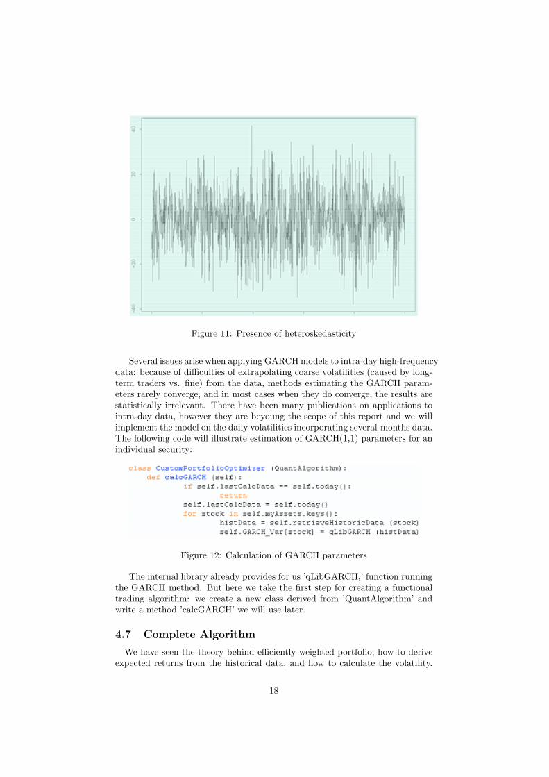
Figure 11: Presence of heteroskedasticity

Several issues arise when applying GARCH models to intra-day high-frequencydata: because of difficulties of extrapolating coarse volatilities (caused by long-term traders vs. fine) from the data, methods estimating the GARCH param-eters rarely converge, and in most cases when they do converge, the results arestatistically irrelevant. There have been many publications on applications tointra-day data, however they are beyoung the scope of this report and we willimplement the model on the daily volatilities incorporating several-months data.The following code will illustrate estimation of GARCH(1,1) parameters for anindividual security:

Figure 12: Calculation of GARCH parameters

The internal library already provides for us ’qLibGARCH,’ function runningthe GARCH method. But here we take the first step for creating a functionaltrading algorithm: we create a new class derived from ’QuantAlgorithm’ andwrite a method ’calcGARCH’ we will use later.

4.7 Complete Algorithm

We have seen the theory behind efficiently weighted portfolio, how to deriveexpected returns from the historical data, and how to calculate the volatility.

18

With GARCH calculation defined above, the following is an implementation ofa portfolio optimizing algorithm:

Figure 13: Portfolio Optimization

5 Future Work

There are several projects I am interested in pursuing after I finish Quant:(1) connecting Quant to an artificial stock market, such as the Santa Fe version,and (2) researching the formal description of financial contracts (options, swaps,etc.) using a functional approach and building an automated system to screenfor arbitrage opportunities.

6 Acknowledgements

I would like to thank Dr. Greg Lavender for his continuing guidance, ex-pertise, and support that made this project a possibility, and Deutsche Bank’sIndex Arbitrage and Quantitative Strategies Groups for the invaluable experi-ences.

References

[1] Lutz, Mark. Programming Python. Sebastopol, California: O’Reilly MediaInc., 2003.

[2] Dacorogna, Michel, Gencay, Ramazan, Mueller, Ulrich, Olsen, Richard,and Pictet, Olivier. Introduction to High Frequency Finance. San Diego,California: Academic Press, 2001.

[3] Reilly, Frank, and Brown, Keith. Investment Analysis & Portfolio Management.Mason, Ohio: Thompson South-Western, 2003.

[4] Bodie, Zvi, Kane, Alex, and Marcus, Alan. Investments. New York: Mc-Graw Hill, 2002.

[5] Harris, Larry. Trading and Exchanges. New York, New York: Oxford Uni-versity Press, 2003.

19

[6] Lutz, Mark and Ascher, David. Learning Python. Sebastopol, California:O’Reilly Media Inc., 2003.

[7] ASPN Python Cookbook. 05 May 2006.<http://aspn.activestate.com/ASPN/Cookbook/Python>

[8] Introduction to R Statistical Package. Venables, W. N. , and Smith, D.M.<http://cran.r-project.org/doc/manuals/R-intro.pdf>

[9] TSeries: Package for time series analysis and computational finance.Trapletti, Adrian, and Hornik, Kurt. <http://cran.r-project.org/src/contrib/Descriptions/tseries.html>

[10] MySQL Commands. 05 May 2006. <http://www.pantz.org/database/mysql/mysqlcommands.shtml>

[11] Insert GARCH material

[12] Probably some other r-package documentation

[13] Kendrick, David, Mercado, Ruben, and Amman, Hans.Computational Economics Modeling. Austin: UT Austin Press, 2005.

[14] Kritzman, Mark. Portable Financial Analyst. New York: Wiley Finance,2003.

[15] Engle, Robert. 2001. GARCH 101: The Use of ARCH/GARCH Models in Applied Econometrics.

[16] Markowitz, Harry. Portfolio Selection. The Journal of Finance, 1952.

20