To my family

List of Papers

This thesis is based on the following papers, which are referred to in the text by their Roman numerals.

I Morell, A., Ahlström, H., Schoenberg, S. O., Abildgaard, A.,

Bock, M., Bjørnerud, A. (2008) Quantitative renal cortical per-fusion in human subjects with magnetic resonance imaging us-ing iron-oxide nanoparticles: influence of T1 shortening. Acta radiologica, 49(8):955–962

II Jonsson*, O., Morell*, A., Zemgulis, V., Lundström, E., Tovedal, T., Myrdal Einarsson, G., Thelin, S., Ahlström, H., Bjørnerud, A., Lennmyr, F. (*equal contribution) (2011) Mini-mal safe arterial blood flow during selective antegrade cerebral perfusion at 20° centigrade. The annals of thoracic surgery, 91(4):1198-1205

III Morell, A., Jonsson, O., Tovedal, T., Zemgulis, V., Myrdal Einarsson, G., Thelin, S., Ahlström, H., Lennmyr, F., Bjørne-rud, A. Sensitivity of dynamic susceptibility contrast MRI to change in global flow rate. Manuscript

IV Morell, A., Lennmyr, F., Jonsson, O., Tovedal, T., Pettersson, J., Bergquist, J., Zemgulis, V., Myrdal Einarsson, G., Thelin, S., Ahlström, H., Bjørnerud, A. Influence of blood/tissue differ-ences in contrast agent relaxivity on tracer based MR perfusion measurements. Manuscript

Reprints were made with permission from the respective publishers.

Contents

Introduction ................................................................................................... 11 Magnetic resonance imaging .................................................................... 11 Spin relaxation .......................................................................................... 13 Contrast agents ......................................................................................... 15 Dynamic susceptibility contrast MRI ....................................................... 18 Tracer particle concentration .................................................................... 23 Laboratory animals ................................................................................... 26

Aim ............................................................................................................... 27 Primary aim .............................................................................................. 27 Specific aims ............................................................................................ 27

Materials and methods .................................................................................. 28 Study I ...................................................................................................... 28 Study II ..................................................................................................... 31 Study III ................................................................................................... 34 Study IV ................................................................................................... 37

Results ........................................................................................................... 42 Study I ...................................................................................................... 42 Study II ..................................................................................................... 43 Study III ................................................................................................... 45 Study IV ................................................................................................... 48

Discussion ..................................................................................................... 55 From signal intensity to relaxation rate .................................................... 56 From relaxation rate to concentration ...................................................... 56 From concentration curves to blood flow and volume ............................. 57

Conclusions ................................................................................................... 60

Acknowledgements ....................................................................................... 62

References ..................................................................................................... 65

Abbreviations

ADC Apparent diffusion coefficient AIF Arterial input function CA Contrast agent CPB Cardio pulmonary bypass DSC-MRI Dynamic susceptibility contrast MRI ECF Extracellular fluid FB Tissue blood flow (ml/100 g/min) or (ml/100 ml/min) GM Grey matter hct Hematocrit MR Magnetic resonance MRI Magnetic resonance imaging R1 Longitudinal relaxation rate, 1/T1 (s-1) r1 T1 relaxivity of contrast agent (s-1mM-1) R2 Transverse relaxation rate, 1/T2 (s-1) r2 T2 relaxivity of contrast agent (s-1mM-1) R2* Effective transverse relaxation rate, 1/T2* (s-1) r2* T2* relaxivity of contrast agent (s-1mM-1) Rapp Apparent relaxation rate (s-1), under influence of

secondary relaxation effects ROI Region of interest SNR Signal to noise ratio SVD Singular value decomposition T/R Transmit receive, type of coil T1 Longitudinal relaxation time (ms) T2 Transverse relaxation time (ms) T2* Effective transverse relaxation time (ms) TE Echo time, sequence parameter (ms) tm Mean transit time (s) TR Repetition time, sequence parameter (ms) USPIO Ultra-small particles of iron oxide, class of contrast

agents VB Tissue blood volume (ml/100 g) or (ml/100 ml) WM White matter

11

Introduction

Organ function, and ultimately cell survival, is dependent on adequate blood supply – the tissue perfusion. For pathologies where the perfusion is locally altered, for example stroke or tumors, a perfusion map is visually straight-forward and an intuitive tool for the radiologist. There are several methods to accomplish these regional perfusion maps and all of them are image based. Basically, the methods can be grouped by three principles; by dynamically monitoring the kinetics of a tracer, statically measuring the absorption of a tracer and collecting images sensitive to blood motion. The modalities avail-able to perform these measurements are computer assisted tomography, sin-gle photon emission computed tomography, positron emission tomography and magnetic resonance imaging (MRI). This work is focused on a method in which the perfusion is assessed by using MRI to observe the transport of a contrast agent bolus through the tissue of interest. The idea is that the ampli-tude and shape of the sampled tracer concentration curves from a feeding artery and the tissue of interest contains the perfusion properties of the tis-sue. This technique is called the first pass method or dynamic susceptibility contrast imaging (DSC-MRI). This sort of impulse response measurement to measure tissue perfusion is not unique for MRI but was in the late 1980’s to early 1990’s adapted to MRI [1-3] from nuclear medicine where it was known as the indicator dilution method [4, 5]. In general, measurements by which a dynamic system is characterized by its response to an impulse is applied in a wide variety of fields - from electric circuits, signal processing and control systems to vibration properties of buildings and geologic inves-tigations.

Magnetic resonance imaging MRI is a remarkable technique to visualize the interiors of the human body and the function of its organs. The success of the technique relies on the continuous efforts of thousands to develop and improve the MR methods, but its existence depends on two fundamental insights. The first, presented in 1946 [6, 7], is the behavior of the hydrogen nucleus, and other particles with a spin angular momentum, in a magnetic field – the magnetization precesses around the magnetic field lines with a frequency proportional to the magnet-

12

ic field. The second, presented in 1973 [8], is the idea to generate images by manipulating the magnetic fields around the hydrogen protons.

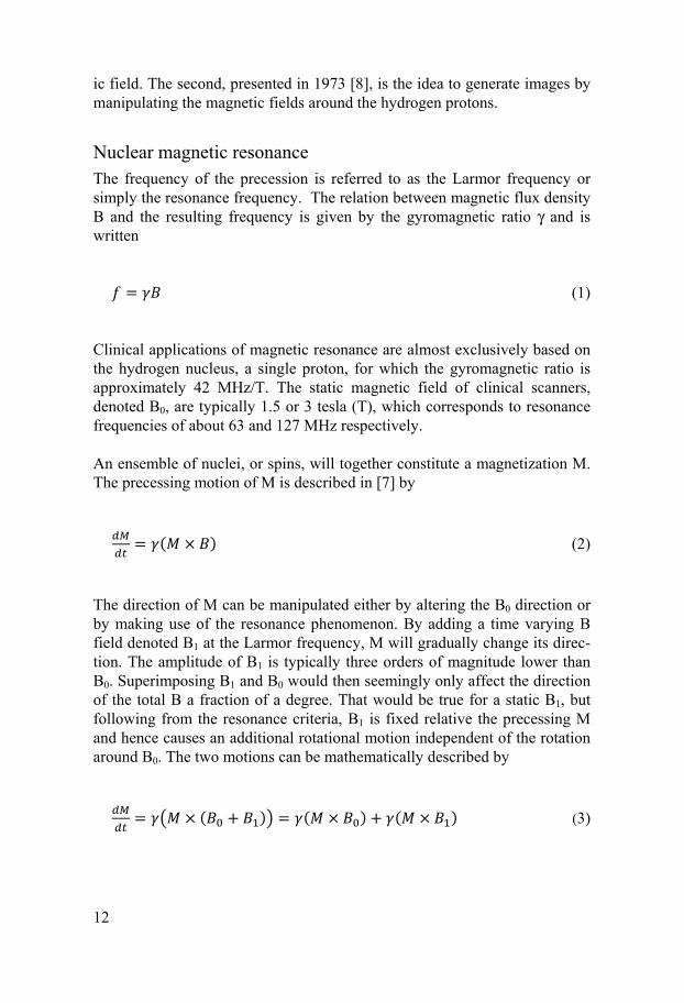
Nuclear magnetic resonance The frequency of the precession is referred to as the Larmor frequency or simply the resonance frequency. The relation between magnetic flux density B and the resulting frequency is given by the gyromagnetic ratio γ and is written

(1)

Clinical applications of magnetic resonance are almost exclusively based on the hydrogen nucleus, a single proton, for which the gyromagnetic ratio is approximately 42 MHz/T. The static magnetic field of clinical scanners, denoted B0, are typically 1.5 or 3 tesla (T), which corresponds to resonance frequencies of about 63 and 127 MHz respectively.

An ensemble of nuclei, or spins, will together constitute a magnetization M. The precessing motion of M is described in [7] by

( ) (2)

The direction of M can be manipulated either by altering the B0 direction or by making use of the resonance phenomenon. By adding a time varying B field denoted B1 at the Larmor frequency, M will gradually change its direc-tion. The amplitude of B1 is typically three orders of magnitude lower than B0. Superimposing B1 and B0 would then seemingly only affect the direction of the total B a fraction of a degree. That would be true for a static B1, but following from the resonance criteria, B1 is fixed relative the precessing M and hence causes an additional rotational motion independent of the rotation around B0. The two motions can be mathematically described by

( ) ( ) ( ) (3)

13

The resulting angle of M relative to B0 depends on the combination of ampli-tude and duration of B1. From a classical point of view, M becomes mag-netically “visible” if it has a component orthogonal to the axis of precession, which is parallel to B0. The transverse component of M is a miniature equiv-alent to the rotating magnet inside a generator which causes a fluctuating electromagnetic field. This emitted field is the magnetic resonance (MR) signal.

Image generation Since the resonance frequency depends on the magnetic flux density B, it is by introducing controlled spatial variations in B, magnetic field gradients, possible to select which protons to excite depending on their location. The same mechanism makes it possible to produce a spatial dependence of the frequency and phase of the excited protons. By applying these magnetic field gradients together with excitation pulses in an intelligent way it is possible to excite and spatially encode groups of protons and thus produce an image.

Spin relaxation As described above, MR images are acquired by manipulating the magnetic orientations of the hydrogen nuclei. Spin relaxation is the process by which the nuclei returns to the resting state after one or several excitation pulses, see Figure 1. The relaxation process is generally treated as two independent processes with one model describing the recovery of the longitudinal mag-netization and one describing the decay of the transverse magnetization.

Figure 1. Illustration of the relaxation processes following a 90 degree excitation pulse for a group of spins.

Longitudinal relaxation The longitudinal relaxation process is the recovery of the longitudinal mag-netization MZ along B0 after being tipped an angle α by an excitation pulse. If MR image sampling consisted of only one echo generated by a single ex-citation pulse, the initial amplitude of the signal would only depend on the spin density. However, since an image is constructed of numerous echoes evenly spaced by the repetition time of the sampling sequence, the rate of

14

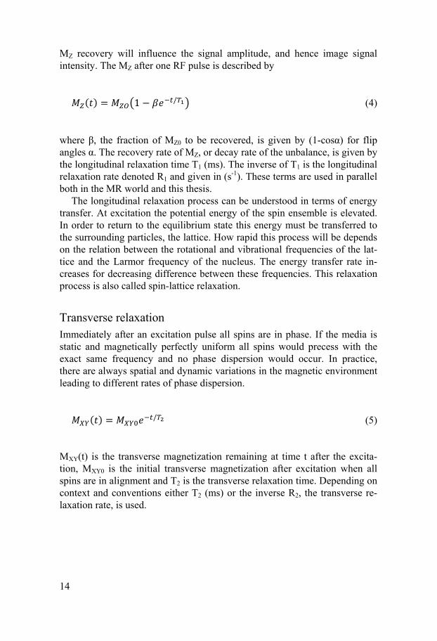
MZ recovery will influence the signal amplitude, and hence image signal intensity. The MZ after one RF pulse is described by

( ) 1 / (4)

where β, the fraction of MZ0 to be recovered, is given by (1-cosα) for flip angles α. The recovery rate of MZ, or decay rate of the unbalance, is given by the longitudinal relaxation time T1 (ms). The inverse of T1 is the longitudinal relaxation rate denoted R1 and given in (s-1). These terms are used in parallel both in the MR world and this thesis.

The longitudinal relaxation process can be understood in terms of energy transfer. At excitation the potential energy of the spin ensemble is elevated. In order to return to the equilibrium state this energy must be transferred to the surrounding particles, the lattice. How rapid this process will be depends on the relation between the rotational and vibrational frequencies of the lat-tice and the Larmor frequency of the nucleus. The energy transfer rate in-creases for decreasing difference between these frequencies. This relaxation process is also called spin-lattice relaxation.

Transverse relaxation Immediately after an excitation pulse all spins are in phase. If the media is static and magnetically perfectly uniform all spins would precess with the exact same frequency and no phase dispersion would occur. In practice, there are always spatial and dynamic variations in the magnetic environment leading to different rates of phase dispersion.

( ) / (5)

MXY(t) is the transverse magnetization remaining at time t after the excita-tion, MXY0 is the initial transverse magnetization after excitation when all spins are in alignment and T2 is the transverse relaxation time. Depending on context and conventions either T2 (ms) or the inverse R2, the transverse re-laxation rate, is used.

15

Contrast agents MR contrast agents are pharmaceutical substances injected intravenously in order to enhance, or generate, differences in signal intensity between tissues or regions in the MR image. This effect of the contrast agent molecules, themselves invisible in the MR image, is due to their power to accelerate the relaxation processes of surrounding native protons. Compared to the contrast agents used in X-ray applications, the mechanisms are fundamentally differ-ent – in an X-ray image the contrast agent itself is depicted. A contrast agent particle consists of a magnetically active component, such as a metal ion, and a carrier component. Together, these two components determine the relaxation properties and the biodistribution of the contrast agent.

The measure of how effectively the contrast agent alters the relaxation rate is described by its relaxivity rε, where ε is 1 or 2 for longitudinal and transverse relaxation respectively. The relaxivity defines how much the re-laxation rate Rε is altered per concentration unit and is written

(6)

R0 is the original relaxation rate in s-1, C the contrast agent concentration in mM and consequently the relaxivity r in s-1mM-1.

There are two mechanisms by which the contrast agent particles affect proton relaxation – dipolar and susceptibility induced relaxation. Dipolar relaxation refers to when a proton magnetically interacts directly with anoth-er particle. Susceptibility induced relaxation refers to the proton being influ-enced by variations in the magnetic field due to the presence of the contrast agent particle.

Chelated gadolinium agents This is the group of contrast agents most frequently used in the clinical set-ting; chelated gadolinium agents or paramagnetic ECF agents. ECF is the abbreviation for extracellular fluid, referring to the distribution volume of the agent in vivo. The size of the chelate enables it to leak out of the intra-vascular volume into the interstitium, except for regions with intact blood-brain barrier. Also due to the low molecular weight, these agents are elimi-nated by glomerular filtration.

Chelation is a form of molecular shield – a single atom, the gadolinium ion, is bound centrally inside a molecule, the ligand DTPA, preventing it to chemically react with the surrounding. Gadolinium(III) is a metal ion, be-longing to the group lanthanides, and it has three properties making it suita-

16

ble for this application. First, it has seven unpaired electrons, each having a magnetic moment of about 650 times that of a proton. Second, the frequen-cies of these electrons are close to the Larmor frequency of the protons lead-ing to effective dipolar relaxation. Third, it binds strongly to the carrier mol-ecule DTPA, an important property both because of the favorable biodistri-bution properties of DTPA but more importantly to reduce toxicity since gadolinium is toxic and must not be released inside the body. Paramagnetism is related to the magnetic susceptibility χ of the agent. For any compound positioned in a magnetizing field H, the induced magnetization M is given by the compounds magnetic susceptibility according to

(7)

For paramagnetic particles χ is positive – the magnetization M is parallel to H and the magnetic field is locally increased. However, when the particle no longer experiences the H field the magnetization M returns to zero.

USPIO blood pool agents USPIO stands for ultrasmall particles of iron-oxide. To qualify as ultrasmall the total particle size should be less than 50 nm. Larger particles, 50-200 nm, are categorized as small (SPIO). Blood-pool refers to the biodistribution – in contrast to the gadolinium ECF agents these particles are too large to leak into the interstitium. Instead they are contained in the intravascular volume. The size also affects the elimination process, instead of being filtrated by the kidneys the USPIO particles are eliminated by the reticuloendothelial system (liver, spleen, bone marrow). The iron oxide particles are crystals made up by thousands of iron ions (Fe2+ and Fe3+). Individually these iron ions are paramagnetic, but magnetically ordered in a crystal structure the magnetic field is “amplified” and the particle is categorized as superparamagnetic.

Dipolar relaxation For gadolinium based agents, the dipolar relaxation is described as three separate processes depending on the distance between the proton and the gadolinium ion – inner, second and outer sphere relaxation respectively. However, the contribution of the second sphere component is usually com-bined with the outer sphere component [9] and the relaxivity of a paramag-netic agent is written

17

(8)

Although the DTPA molecule effectively contains the gadolinium ion, there is one gadolinium correlation site, of totally nine, available for water mole-cules to “magnetically interact” with it. The resulting effect will depend on the relaxation rate of the protons of the correlated water molecule TεM, the residence time of the water molecule τM, the amount of paramagnetic parti-cles P (mole fraction) and correlation sites q [10] and can be mathematically described by

(9)

The term TεM is given by the Solomon-Bloembergen-Morgan equations, a formalism outside the scope of this text. There is an additional correlation process, when a hydrogen proton of the water molecule correlates with an atom of the surface of the ligand, leading to second sphere relaxation. How-ever, as mentioned above, the contribution of this process is usually not treated individually but incorporated the term for the outer sphere relaxation.

For the USPIO agent there is no inner sphere relaxation component due to the molecular design, the surface of the iron oxide core is completely cov-ered by the coating layer and there are no correlation sites available.

Outer sphere relaxation stems from the motion (diffusion) of the bulk wa-ter molecules relative to the contrast agent particle. The molecules are mod-eled as hard spheres and the components included in the calculations are the concentration of the gadolinium complex, the distance of closest approach and the diffusion constants of the molecules [11].

Relaxation due to susceptibility The models of dipolar relaxivity are developed for contrast agents in solu-tions – contrast agent particles surrounded by free bulk water molecules. However, once injected into biological tissue, the contrast agent will be compartmentalized – depending on the biodistribution of the particle and the tissue structure. It is this compartmentalization that gives rise to the suscep-tibility induced relaxation. As the particles are unevenly distributed there will be local spatial variations in the magnetic field. Recalling the fundamen-tal relationship described by Eq. (1), every B distribution results in a corre-sponding frequency distribution and, consequently, the phase dispersion

18

denoted susceptibility induced relaxation. It is a complicated situation to model and theoretical models, numerical simulations and experimental stud-ies have been presented in efforts to elucidate the matter [12-15].

Dynamic susceptibility contrast MRI The DSC-MRI method is basically an impulse response experiment and the system to be characterized is the tissue, or rather the vascular system of the tissue. The impulse is the arterial input function, a bolus of tracer particles, typically induced by venous injection of a gadolinium based MR contrast agent. By running a fast MRI sequence sensitive to the susceptibility effect of these tracer particles it is possible to sample the bolus transport both through the feeding arteries and the tissue. The signal intensity variation in the collected image series due to the contrast agent is converted into estimat-ed contrast agent concentration and are denoted CB(t) for the arterial blood and CT(t) for the tissue – typically one curve for each image pixel. There is a number of conditions that must be fulfilled in order for the method to be valid and below follows a selection;

1. The hemodynamic properties of the tracer particles should be identical to bulk blood, i.e. restricted to the intravascular space

2. Ability to accurately measure the tracer particle concentration. 3. The system must be closed, in the sense that any blood or tracer

particle entering the system must also eventually leave the system. 4. The system must be stationary, that is it must not change volume

or flow properties during the measurement

Condition 4 is generally considered fulfilled. Condition 3 and 1 are compli-cated since the major applications of perfusion studies is the study of region-al pathologies such as tumors or areas affected by infarction and it may well be that the vessels in these regions have a reduced quality and leaks tracer particles into the extravascular space. There are methods to estimate this leakage, but it is an inherent weakness of the method. Common to the condi-tions so far is that the fulfillment of them depends on the vascular system itself and is independent of modality. Condition 2 however is of a different kind, it is instead dependent on the measurement technique and concentra-tion measurements are classically a problematic area in MR applications. When performing DSC-MRI perfusion condition 2 is normally handled with the assumption of linear and identical contrast agent relaxivity in blood and all relevant tissues. The consequences of these assumptions are one of the main topics of this thesis and are treated in Study I and IV.

19

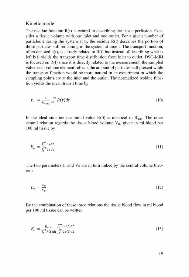
Kinetic model The residue function R(t) is central in describing the tissue perfusion. Con-sider a tissue volume with one inlet and one outlet. For a given number of particles entering the system at t0, the residue R(t) describes the portion of those particles still remaining in the system at time t. The transport function, often denoted h(t), is closely related to R(t) but instead of describing what is left h(t) yields the transport time distribution from inlet to outlet. DSC-MRI is focused on R(t) since it is directly related to the measurement, the sampled value each volume element reflects the amount of particles still present while the transport function would be more natural in an experiment in which the sampling points are at the inlet and the outlet. The normalized residue func-tion yields the mean transit time by

( ) (10)

In the ideal situation the initial value R(0) is identical to Rmax. The other central relation regards the tissue blood volume VB, given in ml blood per 100 ml tissue by

(11)

The two parameters tm and VB are in turn linked by the central volume theo-rem

(12)

By the combination of these three relations the tissue blood flow in ml blood per 100 ml tissue can be written

( ) ( )( ) (13)

20

Practically, the contrast agent particles are distributed in the blood plasma, so the fraction of the total intravascular volume available for the tracer parti-cles is (1-hct) where hct is the hematocrit. Since hct differs between large and small vessels, for which CB(t) and CT(t) are measured, this difference is corrected for by multiplying the right hand side of both Eq. (11) and Eq. (13) with the factor khct = (1-hctlarge) / (1-hctsmall).

The ideal arterial input function, which would be an impulse or Dirac function – a function of amplitude 1 and infinitesimal width – would pro-duce a tissue response identical to R(t). In practice however, the input func-tion have a spatial and temporal width and the observed tissue response CT(t) can mathematically be described as a convolution of the input and the resi-due functions ( ) ( ) ∗ ( ) ( ) ( ) (14)

The residue R(t) is extracted from CT(t) and CB(t) by a deconvolution opera-tion [16, 17].

Relative blood volume obtained at different locations in tissue supplied by the same AIF can be estimate directly from the tissue response as reduc-ing Eq. (11) to ∝ ( ) (15)

Similarly, relative perfusion is commonly estimated according to ∝ max ( ) (16)

under the assumption that the AIF is identical for all tissues of interest and further that the AIF has a sufficiently short duration allowing R(t) to be ap-proximated directly by CT(t).

Deconvolution methods The methods to perform the deconvolution can be divided into two groups depending on whether or not they use assumptions or a priori knowledge of the tissue vasculature.

21

Model dependent methods These methods rely on a priori knowledge or assumptions of the vascular system. It means that the mathematical solution is restricted to fit into a cer-tain set of boundaries - conditions that can guarantee a physiologically plau-sible solution. However, it is important to keep in mind that by defining the-se constraints, the quality of the result depends on how well the model corre-sponds to the actual vasculature. Abnormal signal behavior, which may be the result of pathology, may be forced into a normal physiologic pattern.

An example of such a model is to use one or a combination of several ex-ponential terms to describe the impulse response. One single exponential term corresponds to a single, instantaneously well mixed compartment.

Model independent methods Here a more strictly mathematical solution is produced. In principle it does not rely on any assumptions of the vascular structure or hemodynamics, but in practice some sort of condition must be included to promote “well be-haved” solutions, e.g. suppress oscillations and negative values.

The most widely used and established method in this group is the singular value decomposition method (SVD). The components of the convolution equation are written in matrix form and the equation is solved by linear alge-bra [17]. Eq. (14) is rewritten in matrix form;

(17)

Where A and b are the observed arterial and tissue responses

C (t ) 0C (t ) C (t ) … 0… 0⋮ ⋮C (t ) C (t ) ⋱ ⋮… C (t ) (18)

C (t )C (t )⋮C (t ) (19)

22

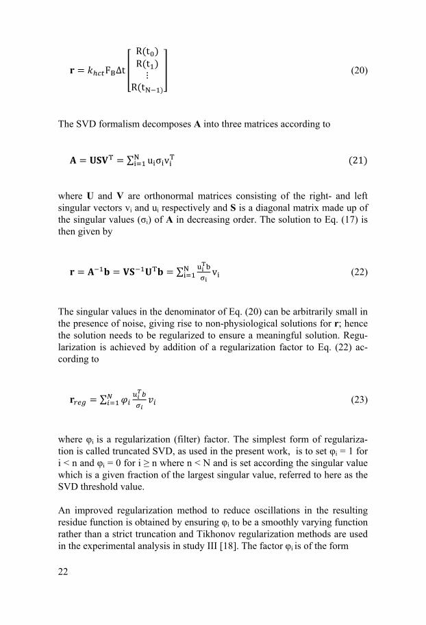
F ∆t R(t )R(t )⋮R(t ) (20)

The SVD formalism decomposes A into three matrices according to

∑ u σ v (21) where U and V are orthonormal matrices consisting of the right- and left singular vectors vi and ui respectively and S is a diagonal matrix made up of the singular values (σi) of A in decreasing order. The solution to Eq. (17) is then given by ∑ v (22)

The singular values in the denominator of Eq. (20) can be arbitrarily small in the presence of noise, giving rise to non-physiological solutions for r; hence the solution needs to be regularized to ensure a meaningful solution. Regu-larization is achieved by addition of a regularization factor to Eq. (22) ac-cording to

∑ (23)

where φi is a regularization (filter) factor. The simplest form of regulariza-tion is called truncated SVD, as used in the present work, is to set φi = 1 for i < n and φi = 0 for i ≥ n where n < N and is set according the singular value which is a given fraction of the largest singular value, referred to here as the SVD threshold value.

An improved regularization method to reduce oscillations in the resulting residue function is obtained by ensuring φi to be a smoothly varying function rather than a strict truncation and Tikhonov regularization methods are used in the experimental analysis in study III [18]. The factor φi is of the form

23

φ (24)

where λ is a regularization parameter controlling the relative weighting of each singular value.

A computationally less exhaustive approach is to mathematically transform the components into another domain in which the deconvolution operation is reduced to a much less complicated mathematical operation [16]. In the Fou-rier domain, for example, the equivalents of convolution and deconvolution are multiplication and division respectively.

Tracer particle concentration The DSC-MRI formalism requires dynamic tracer particle concentration measurements, both in arterial blood and in tissue. Converting observed sig-nal intensity variations S(t) into corresponding variation in contrast agent concentration C(t) is principally a two-step process.

∆ ( ) → ∆ ( ) → ∆ ( ) (25)

Assumptions and considerations regarding these two steps are given below.

From signal to relaxation rate The signal dependence for spoiled gradient echo sequences is written

( ) ∝ ∙ ( )∙ ∙ ( ) exp ∙ ′( ) (26)

The sequence parameters which defines the contrast properties of the ac-quired images are the repetition time TR, the echo time TE and flip angle α. R1(t) and R2’(t) denotes the longitudinal and transverse relaxation rates re-spectively. In principle, the signal depends on two components affected by R1 and R2’ respectively;

24

( ) ∝ sin ∙ ( ) ∙ ′( ) (27)

A contrast agent have both R1 and R2’ properties, and depending on choice of method one of them is considered the primary relaxation process while the other is secondary. This means that the MR acquisition is optimized to reflect the variation in the primary relaxation while the secondary is assumed to have negligible influence on the measurements. Considering Eq. (27) above either E1 or E2 is assumed constant.

For T1-based perfusion, a saturation recovery type sequence has been suggested as an alternative to gradient echo but the signal response can also be modeled by Eq. (26) by using α=90o and replacing TR with TD, the delay time between the initial 90° pulse and the center of k-space readout [19]. In T1-based perfusion analysis, the E2’(t) term is assumed to be negligible when converting change in signal intensity to change in R1 and the change in R1 is given by: ∆ ( ) ( )∙ ∙( )∙ (0) (28)

where ( )( ) ( )( ) (29)

Assuming negligible change in R2’ Eq. (29) is reduced to x = S(t) / S(0). In T2- and T2*-based perfusion analysis, the corresponding change in R2’ is given by:

Δ ′( ) ( )( ) ( )( ) (30)

∆R2’(t) is commonly estimated by assuming E1(t) ≈ E1(0), but for signifi-cant T1-effects E1(t) >> E1(0) so that ∆R2’(t) is under-estimated by a factor given by

( )( ) (31)

25

The error introduced due to neglecting the secondary relaxation effects will depend on both the sequence parameters and the CA concentration range.

From relaxation rate to CA concentration The second step regards translating the estimated ΔR(t) into ΔC(t). In tracer based perfusion measurements the relation between the observed change in relaxation rate and the underlying change in CA concentration is assumed to follow ∆R r ∆C (32) where Rε is one of the relaxation rates R1, R2 and R2* in s-1, rε is the corre-sponding CA relaxivities r1, r2 and r2* in s-1mM-1 and C the CA concentra-tion in mM. Eq. (32) is well suited to describe the observed effect in homo-geneous media such as aqueous solutions but it is well known that the tissue heterogeneity have a large influence on relaxation properties [12, 13]. Con-sidering the situation in impulse response perfusion measurements, the main assumption is not regarding the linearity but rather that blood and all tissues having identical relaxivity. The impact of non-identical relaxivities on perfu-sion measurements may be described by substituting the CA concentration C in the previously presented perfusion equations by the relaxation rate as giv-en by Eq. (32). Denoting blood and tissue relaxivity by rB and rT respective-ly, the tissue blood volume in Eq. (11) can be written

V ∆ ( )∆ ( ) ∆ ( )∆ ( ) (33)

Analogously, tissue blood flow in Eq. (13) can be written

( ) ∆∆ ( ) ∆∆ (34)

According to these relations, VB and FB are equally affected by this scaling factor. The mean transit time tm, being defined as the VB/FB is not affected at all. The tissue relaxivity as measured relative to blood concentration will be

26

denoted r while the relaxivity relative to tissue concentration is denoted by rT, or rbvc for blood volume corrected tissue relaxivity. It should be noted that R(t=0) may not coincide with Rmax due effective time shifts between the AIF and tissue response in a given tissue location. The influence of these time shifts on perfusion measurements have been described and there are strate-gies to correct for this effect [20, 21].

Laboratory animals A major part of the data presented in this thesis was generated in an experi-ment in which laboratory animals were used, in this case pigs. Using animals in medical research is a matter highly regulated by law and under supervi-sion from authorities. However, laws and formalism aside, it brings im-portant ethical dimensions to the research. All experiments involving labora-tory animals are formally reviewed regarding the three R’s which stand for Replacement, Reduction and Refinement. This principle was described in 1959 by Russell and Burch [22], it gained ground during the 1970’s and is today, although interpreted a bit differently, fundamental in all work regard-ing laboratory animals. In short, today the three R’s stand for

• Replacement, if possible animal experiment must be replaced with an alternative method.

• Reduction, the experiment must be performed with as few animals a possible.

• Refinement, the experiment must be designed to cause as little discomfort as possible to the animal.

The main objective of the current experiment was the clinical problems ob-served almost daily of patients suffering from neurological symptoms after surgical procedures involving cardio pulmonary bypass (study II). No animal in this study experienced any other intervention than the injection inducing anesthesia at arrival to the site. The two following studies in this thesis re-garding DSC-MRI properties and contrast agent dose response is based on data collected during the original experiment and did not lead to use of addi-tional animals or inflict any discomfort for the animals

27

Aim

Primary aim The primary aim of this work was to study the feasibility of obtaining quan-titative estimates of perfusion related parameters using tracer based MRI perfusion methods.

Specific aims Study I Study the feasibility of DSC-MRI for kidneys using an iron oxide based contrast agent and the influence of secondary relaxation effects on the DSC-MRI measurements.

Study II Implement and generate gadolinium based DSC-MRI data in pigs undergo-ing cardio pulmonary bypass procedure and study the influence of CPB blood flow rate on risk factors for developing cerebral ischemia.

Study III Study the ability of DSC-MRI to measure variations in global changes in blood flow by experimental measurements in pigs undergoing cardio pulmo-nary bypass procedure and through numerical simulations.

Study IV Study the in vivo relaxivity properties of a gadolinium based contrast agent and estimate the influence on tracer based MRI perfusion measurements of differences in blood/tissue relaxivity and secondary relaxation effects.

28

Materials and methods

Study I Study design The patients underwent one renal DSC-MRI with an iron oxide contrast agent. The study was performed at three different centers; DKFZ Heidel-berg, Germany (H), Rikshospitalet University Hospital, Oslo, Norway (O) and Uppsala University Hospital, Uppsala, Sweden (U). The study was part of a phase II clinical trial for the iron oxide contrast agent. The trial was approved by respective regional ethics committee and informed consent was obtained from all patients recruited for the study.

Population Ten patients with confirmed unilateral renal artery stenosis were included in this study; four of these were later excluded after examination of the MR images, see Results section for details. The ten patients were distributed among the centers as follows; H five patients, O one patient and U four pa-tients. The status of the renal arteries was determined by X-ray angiography and kidneys with no significant renal artery stenosis were considered normal.

MR imaging

A single slice double–echo gradient echo sequence with temporal resolution of 1 second was used, i.e. every second two images with different TE were generated for the same slice. The slice was oriented to include both kidneys and a section of the abdominal aorta. In order to eliminate the normal breath-ing induced motion of the kidneys, imaging was performed during breath-hold. A selection of imaging parameters: TR/TE1/TE2/flip/voxel size = 11.7 ms / 4.5 ms / 9.0 ms / 12° / 2.75 × 2.72 × 6.0 mm3 (H and O) and 11.8 ms / 3.4 ms /9.0 ms /12° / 1.37 × 1.37 × 6.0 mm3 (U). All imaging were per-formed on clinical 1.5 T MR-systems; Magnetom Vision Plus (Siemens Medical Solutions, Erlangen, Germany) (H and O) and ACS Intera (Philips Medical Systems, Best, The Netherlands) (U). The contrast agent was manu-ally injected as a rapid bolus at a dose of 1.25 mg Fe/kg body weight.

29

Contrast agent The contrast agent (NC100150 Injection, GE Healthcare, Oslo, Norway), is a superparamagnetic monocrystalline iron oxide particle based contrast agent. The contrast agent is cleared from the blood by the reticuloendothelial sys-tem, mainly in liver, spleen and bone marrow, with no uptake or filtration in the kidneys. The plasma half-life of the contrast agent is approximately 2.5 h in humans [23].

Data analysis Signal conversion The first step in the analysis was to convert the contrast agent induced signal change into corresponding change in R2* for all pixels. The R2* conversion was performed for both single and double echo data according to previously described methods assuming mono-exponential decay and a linear relation between contrast agent concentration and R2* [24]. For single echo data, assuming T1-effects to be negligible, the change in R2* is given by: ∆ ∗( ) ( )( ) (35)

S(0) and S(t) are the pixel signal intensities at baseline, when no contrast agent is present, and at time t respectively. For double echo data absolute R2* values were calculated by

∗ ( / )

(36)

S1 and S2 are the pixel signal intensities at echo times TE1 and TE2 respec-tively.

Perfusion parameters Regional blood flow, regional blood volume and mean transit time was cal-culated pixel-wise for both single and double echo data following the meth-od described in the introduction, Eqs. (11-13). The correction factor to ac-count for tissue density and the difference in hematocrit between large ves-sels and capillaries were set to 0.705 [16]. Deconvolution was performed with the SVD method with threshold value set to 0.2.

The AIF was sampled in single echo data only (TE1) in the visible section of the abdominal aorta and a gamma-variate fit was used in order to avoid

30

influence of recirculation. The AIF was visually inspected for signal satura-tion and if saturation was evident the data set was excluded.

In order to estimate the total cortical perfusion, the cortical tissue was segmented by manually defining maximum and minimum intensity thresh-olds in ΔR2* maps.

The perfusion parameters were measured in the normal kidneys. The breath-hold approach worked well and no motion correction was required.

All image processing was performed using a commercial software pack-age (nordicICE, NordicNeuroLab, Bergen, Norway).

Estimation of T1 influence on single echo AIF Due to the large difference in R2* effects in the aorta and the renal cortex only the first echo (TE1) was used to calculate ΔR2* for the AIF - for the second echo (TE2) the signal in the aorta was saturated at bolus peak concen-trations. This makes the sampled AIF susceptible to T1 influence, the impact on the R2* response was estimated by simulating the signal response to bo-luses with different peak concentrations.

The simulation consisted of three steps 1) Generate a gamma variate shaped concentration-time curve,

C(t), which simulates the actual bolus concentration 2) Calculate the corresponding signal intensity curves S(t) for a

spoiled gradient echo sequence with echo times TE1 and TE2. 3) Based on the S(t) curves from step (2), calculate and compare

the corresponding R2*(t) response curves for single and double echo acquisitions with Eq. (35) and Eq. (36) respectively.

The relative signal intensity was estimated using the standard expression for spoiled gradient echo sequences, see Eq. (26). The blood relaxation rates were calculated with Eq. (37) and Eq. (38) from in vivo measurements in pig [25].

∗ 111 114 17 (37)

13.9 (38)

R1 and R2* are given in s-1, Cp is plasma concentration in mM and is con-verted to blood concentration by C = (1-hct)·Cp. A baseline T1 in blood of 1 500 ms was used in the simulation. The simulation was performed for five different peak concentrations; 4, 3, 2, 1 and 0.5 mM.

31

Statistical analysis The difference between perfusion parameters based on single and double echo data was statistically analyzed with single sample t-test. Confidence intervals were calculated for 95% and differences yielding p-values of 0.05 or less were considered significant.

Study II Pigs were used to assess the consequence of lowering the blood flow during cardio pulmonary bypass procedure. Several markers of the status of the animals were continuously monitored during the experiment, one being the cerebral perfusion monitored by DSC-MRI.

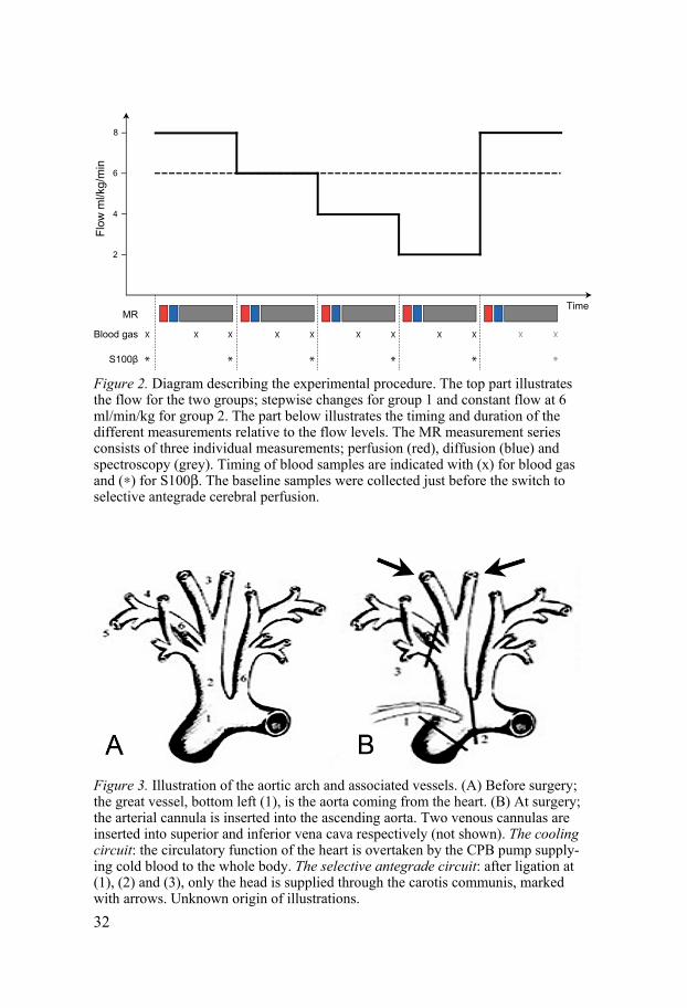
Study design The animals were divided into two groups; in group 1 (n=6) the blood flow was stabilized at blood flow levels 8, 6, 4, 2 and 8 ml/kg/min, where kg re-fers to body weight. In group 2 (n=5) the blood flow was kept constant at 6 ml/kg/min. At each flow level, and at corresponding times for group 2, a series of measurements was performed; MR perfusion, MR diffusion, MR spectroscopy, blood gas analysis and protein S100β. The time needed for each such measurement series was approximately 45 min, see Figure 2 for a schematic illustration of the experiment. The project was approved by the Uppsala Ethical Committee for Animal Research and human care was taken in compliance with the European Convention on Animal Care.

Animal model The pigs were of mixed breed of Hampshire, Yorkshire and Swedish land-race weighing 37.3±3 kg (32.5 – 42 kg). Two different cardio-pulmonary bypass circuits (CPB) were established, see Figure 3; one during preparation and one during the experiment. The first circuit included the whole body, the CPB pump and a blood cooler. The purpose of the first circuit was to effec-tively lower the temperature in the whole body in order to reduce the metab-olism to a minimum. When a core temperature of 20°C was reached, the circuit was modified to only include the head and the CPB pump, see illus-tration below. This circuit is called selective antegrade perfusion circuit. The procedure is common practice in the clinical situation.

The animals were anesthetized at arrival to the facility and the anesthesia was maintained continuously until sacrificed by an intravenous injection of potassium chloride at the end of the experiment.

32

Figure 2. Diagram describing the experimental procedure. The top part illustrates the flow for the two groups; stepwise changes for group 1 and constant flow at 6 ml/min/kg for group 2. The part below illustrates the timing and duration of the different measurements relative to the flow levels. The MR measurement series consists of three individual measurements; perfusion (red), diffusion (blue) and spectroscopy (grey). Timing of blood samples are indicated with (x) for blood gas and (∗) for S100β. The baseline samples were collected just before the switch to selective antegrade cerebral perfusion.

Figure 3. Illustration of the aortic arch and associated vessels. (A) Before surgery; the great vessel, bottom left (1), is the aorta coming from the heart. (B) At surgery; the arterial cannula is inserted into the ascending aorta. Two venous cannulas are inserted into superior and inferior vena cava respectively (not shown). The cooling circuit: the circulatory function of the heart is overtaken by the CPB pump supply-ing cold blood to the whole body. The selective antegrade circuit: after ligation at (1), (2) and (3), only the head is supplied through the carotis communis, marked with arrows. Unknown origin of illustrations.

Flow

ml/k

g/m

in

2

4

6

8

MR

Blood gas

S100β

Time

XX X X X X

*

X

*

X

*

X

*

X

*

X

*

33

MR imaging and spectroscopy MR imaging and spectroscopy was performed with a clinical 1.5T whole body scanner (NT-Intera, Philips Medical Systems, Best, The Netherlands) with a T/R head coil. The pigs were positioned supine in the scanner. For perfusion and diffusion imaging, as well as a set of morphological images, identical geometrical parameters were used in order to facilitate registration between the data sets; acquired voxel size and matrix were 1.67×1.67×4 mm3 and 96×96×12 respectively. The images were oriented to correspond to transverse images of the human brain.

MR perfusion Perfusion data sets were acquired using a gradient echo sequence with single shot EPI readout, temporal resolution 1.6 s and echo time 40 ms. A MRI compatible power injector (Spectris, Medrad, Warrendale, USA) was used for the contrast agent bolus injection (Gadodiamide, GE Healthcare AS, Oslo, Norway). It was connected to the distal end of the arterial cannula through a one-way valve. The contrast agent was diluted 1+1 with isotonic water and well mixed, injection volume 2 mL and flow rate 0.5 mL/s.

MR diffusion Diffusion data sets were acquired using a spin echo sequence with single shot EPI readout, diffusion encoding in three orthogonal directions and b-values 0 and 750 s/mm2.

MR spectroscopy For the single voxel spectroscopic data a PRESS pulse sequence was used to collect 16 non-water-suppressed and 128 water-suppressed scans with repeti-tion time 5000 ms, echo time 22 ms, typical voxel size 20×20×30 mm3, spectral bandwidth 1000 Hz, 1024 points and 16 phase cycle steps. The voxel was positioned central in the cerebrum, thus avoiding the cerebellum and skull bone.

MR image and spectroscopy analysis For each perfusion data set four sets of parametric images were calculated; relative blood flow, relative blood volume and mean transit time. The re-gional signal change during the contrast agent passage was transformed to relative concentration curves, assuming a linear response between contrast agent concentration and R2*. FB was assumed proportional to the maximum of this curve, VB to the area under the curve and tm to the quotient of VB/FB [24]. For each diffusion data set, parametric images of apparent diffusion coefficient (ADC) were calculated. For each subject, all parametric maps were co-registered to the first volume of the first perfusion data set. All par-

34

ametric images were visually inspected to detect any regions of deviating perfusion and diffusion developing during the experiment. tm was measured for the whole brain while ADC was measured for basal ganglia, cortex and whole brain. Image processing regarding perfusion, diffusion and co-registration was performed using a commercially available software package (nICE, NordicNeuroLab, Bergen, Norway). The spectroscopic data was pro-cessed by linear combination of model spectra (LCModel).

Physiologic and hemodynamic monitoring Blood gas Blood samples for venous oxygenation saturation (SvO2), arterial oxygena-tion saturation (SaO2), oxygen pressure PO2, pH, BE (base excess) and Hct were drawn twice during each measurement series – in the middle and at the end of the series plus one at baseline.

S100-beta Blood sample for protein S100β analysis was collected in the beginning of each measurement series, totally five samples per subject.

Blood lactate Lactate analysis performed on blood sample for blood gas.

Study III This study comprises both experimental measurements and numerical simu-lations. The experimental measurements are a subset of the measurements performed in Study II [26].

Experimental measurements In the present study, a subset of the collected perfusion data sets in study II was used where animals with identified pathologies or other physiologic abnormalities following the surgical intervention were excluded. Inclusion criteria were as follows: i) normally appearing perfusion pattern by visual inspection, i.e. laterally symmetric perfusion with no noticeable deviating regions, ii) identifiable AIF in approximately the same region for all animals and iii) AIF detectable in the same anatomical location (same artery) for the different flow levels for each animal. Following these criteria, the flow group was reduced to five subjects at CPB flow levels 8, 6 and 4 ml/kg/min. The control group was by the same criteria reduced to two subjects. The project was approved by the Uppsala Ethical Committee for Animal Re-

35

search and human care was taken in compliance with the European Conven-tion on Animal Care.

Image analysis Regional perfusion maps for FB, VB and tm were calculated with and without use of an AIF, denoted with prefixes q and r for quantitative and relative respectively. Without AIF, rVB and rFB were estimated by Eq. (15) and Eq. (16) and rtm as the ratio rVB/rFB. With AIF, qVB was estimated by Eq. (11) qFB by Eq. (13) and qtm by the ratio qVB/qFB. The quantitative maps were calculated with gamma variate curves fitted to both AIF and the tissue re-sponse. This was done in order to reduce sensitivity to noise and signal satu-ration in blood at high CA concentrations. Deconvolution was performed using singular value decomposition (SVD) with Tikhonov regularization and a fixed threshold of 0.2 [18]. The AIF was sampled with a square region of interest (ROI) with dimensions 2×2 pixels. The position of the AIF sampling ROI was manually adjusted between measurement series, a translational shift generally in the order of one pixel. The sampled AIF was corrected for partial volume effect by assuming equal integral values of an AIF and the corresponding venous outflow function [27]. The venous curves were also sampled with a 2×2 pixels ROI manually positioned in the sagittal sinus. Small variations in position between some of the measurement series were observed, probably due to a combination of surgical adjustments, table movements and the relatively long time between the perfusion measurements (up to 1 h). These variations were corrected for by registering all parametric maps of each subject to a subject specific geometric template – the first dy-namic volume of the first perfusion series. The brain was manually segment-ed with the same EPI template image that was used for registration. A vessel mask was created for each subject based on thresholding in the CBF maps from the first perfusion measurement (at 8 ml/kg/min) in combination with visual inspection of the corresponding dynamic calculated R2* data. The vascular threshold level was adjusted so that equal relative cerebral volume was excluded for all subjects (11.4-11.6%) assuming similar vascular struc-ture in the subjects. All experimental image analysis was performed with a commercially available software package (nordicICE, NordicNeuroLab AS, Bergen, Norway).

Simulated experiments A model was constructed to numerically simulate the process of monitoring a bolus transport through a vessel network.

36

Model design The model consisted of three main compartments in series; a single feeding artery, tissue containing a number of capillaries and a single draining vein. The vascular network had two nodes, one arterial and one venous, at which all capillaries were connected. For each of the three main compartments, a sampling window corresponding to an imaging slice was defined by position and width. The artery and the vein were defined by inner radius and length. The tissue compartment was defined by the number of capillaries and mean values for length and radii. Each capillary was defined by one radius and three sub-compartment lengths; before, within and after the sampling win-dow. The capillary radii and the three sub-segment lengths were randomized following Gaussian distributions given mean length and variance. The arteri-al flow was distributed among the capillaries by relative fluid resistance R calculated by Eq. (39) given by Poiseuille’s law. R (39)

The parameters r and λ are the capillary radius and length respectively. Fur-ther, the tissue sampling window was segmented into a number of sub-volumes, corresponding to image pixels. In the current study the tissue blood volume and flow were varied among the sub-volumes by applying a linear distribution of the number of capillaries with a 1:2 ratio. Tracer injection was defined by shape (modelled by a gamma variate function in the current study), injection duration and dose. The tracer was regarded as ideal point particles added to the blood as it passed the injection site. Plug flow was assumed, hence no dispersion effects were included apart from what resulted from capillary radius, length and flow distributions. The sampled signals were assumed ideal, in the sense that they accurately reflect particle concen-tration in blood and tissue. Hence no influence of relaxivity properties or other sequence related factors were taken into account. After construction of vessel paths and determination of flow distribution of capillary flow, the calculations consisted of following the stepwise transport of the tracer parti-cles. The spatial length of each step dxi of the particles in path i was defined by the global time increment step dt, the flow Fi and radius ri. Tracer particle distribution at the arterial node after an arterial injection was distributed in proportion to the blood flow.

Simulation settings In order to cover the experimental flow range, in which three CPB flow lev-els with ratios 4:6:8 were used, the simulations were performed at estimated corresponding levels 3:9. A total of 7 500 vessels, mean radius 0.2 mm and

37

mean length 160 mm within the sample window, were used. The variation in sample window vascular volume following from integer number of capillary volume elements within the sample window were below 0.1% (maximum difference to mean value).

Analysis of simulated data Relative simulated perfusion data rFB, rVB and rtm were analogously to the analysis of the experimental data acquired using Eq. (15), Eq. (16) and Eq. (12). qVB was calculated with both Eq. (11) and a combination of Eq. (10) and Eq. (12) for estimation of influence of the residue analysis and tm was as before calculated by Eq. (12). qFB was estimated from the maximum value of the tissue residue function obtained by deconvolving the AIF from arrival time adjusted tissue response curves with the truncated SVD deconvolution method. The calculations were performed with four different SVD threshold values; 0.01, 0.05, 0.1 and 0.2. Numerical simulations and analysis of simu-lation data sets were implemented in Matlab (The MathWorks Inc., Natick Massachusetts, USA).

Study IV The data in the current study was collected during the experimental proce-dure in study II [26] by performing steady state concentration level CA dose-response measurements at the end of the experiments in Study II in four animals. The project was approved by the Uppsala Ethical Committee for Animal Research and human care was taken in compliance with the Europe-an Convention on Animal Care.

Experimental design The contrast agent concentration was increased stepwise by repeated injec-tions into the blood circuit. After each injection, which was performed at two opposite sites of the blood circuit simultaneously in order to reach equilibri-um concentration quicker, there was a five minute waiting period before the relaxivity measurements were performed. For each concentration level, three relaxation measurement scans was performed to acquire data for R1, R2 and R2* analysis. In the middle of each scan, an arterial blood sample was col-lected from the arterial cannula in order to determine the absolute gadolini-um concentration in blood. The number of samples with different concentra-tion levels varied between the subjects (4, 5, 9, 9). The injection pattern was designed so the last measurement point corresponded to a total injection volume of 160 ml. One subject received two additional injections of 40 mL each, resulting in a total injected volume of 240 ml.

38

Contrast agent A standard gadolinium chelate (Gadodiamide, GE Healthcare, Oslo, Nor-way) was used. The agent is distributed to the whole extracellular fluid vol-ume with exception of cerebral tissue with intact blood brain barrier. The agent is normally eliminated by renal excretion through glomerular filtration.

MR imaging The MR data acquisitions were performed on a clinical 1.5T whole body scanner (NT-Intera, Philips Medical Systems, Best, The Netherlands) with a single channel T/R head coil. The pigs were positioned supine and the imag-es were oriented to correspond to transverse images of the human brain. All measurements of R1, R2 and R2* were performed with the same geometric parameters; a single slice through a central section of the brain, acquired voxel size was 1.67×1.67×4 mm3 with a 85% rectangular field of view of 160 mm. R1-analysis was performed using a Look-Locker sequence [28] with 70 phases; first inversion time 15 ms, then incrementally increased by 51.7 ms; TE 2.6 ms; TR 6 000 ms; flip angle 6°. R2-analysis was performed using a multi echo turbo spin echo sequence with uniform echo spacing ΔTE. For each measurement 10 images with different TE were acquired with TE = n×ΔTE ms for n = (1, 10) and ΔTE in the range from 30 to 12 ms; TR 2 000 ms and flip angle 90°. In order to acquire a rational sampling range relative to the signal decay curve, the ΔTE was adjusted throughout the experiment. The adjustments were based on the signal decay curve for a region of interest drawn in each image series at the scanner console. Analogous to the R2 measurement, the R2* signal decay curve was sampled by collecting a series of images with different TE with a gradient echo sequence with single shot EPI readout with shifted echo times. Six images were collected with TE = (3.4 + n×ΔTE) ms for n = (0 - 5) and ΔTE in the range from 30 to 3 ms; TR= 2 000 ms and flip angle 15°. The echo spacing was adjusted with increasing Gd concentration in the same way as for the R2 measurements.

Image analysis Relaxation rates were estimated pixel-wise from the respective image series using a non-linear least squares routine, resulting in quantitative R1, R2 and R2* maps at each CA concentration level. The brain was segmented by manual delineation in the baseline (pre-contrast) series. White matter (WM) and gray matter (GM) templates were defined by thresholding in the baseline R1-map, R1 intervals in s-1 for GM and WM were set to [0 - 0.90] and [1.10, max] respectively. Blood vessels were removed from the GM and WM tem-plates by a vessel template defined by R2* thresholding assuming equivalent

39

relative vascular volume. In series with a high and similar CA concentration level of approximately 18mM, a R2* threshold was set to discriminate 15% of the cerebral pixels with highest R2* values. For brain tissue analysis, the GM and WM templates were applied to registered relaxation rate maps. For blood relaxation analysis, a quadratic ROI of size 2×2 pixels, was manually placed in the sinus vein in each of the collected series And the signal intensi-ty curves for this ROI was then used to calculate R1, R2 and R2* values for blood. All image processing and analysis was performed with a dedicated commercial software package (nordicICE, NordicNeuroLab, Bergen, Nor-way).

CA concentration and relaxivity analysis Gd concentration in plasma samples was measured with a SpectrocirosCCD Inductive Coupled Plasma Atom Emission Spectrometer (ICP-AES). Argon was used as plasma and carrier gas at the following rates: plasma, 14 L/min; auxiliary, 0.9 L/min; nebulizer, 0.9 L/min. Applied nebulizer and torch were Mod. Lichte and Fassel respectively. Induction coil was set to a power of 1400 W. Sample flow rate was 1.5 mL/min. The Gd concentration values for each sample was determined from the mean of three measurements and the variation was consistently less than 1%. In order to reduce the risk for sys-tematic errors, four independent wavelengths were used (342.247, 335.047, 336.223, 335.862). The plasma samples were diluted 1 to 10 in MQ-filtered water before measurement and homogenized by means of a Vortex mixer. Plasma concentration values were converted to whole blood concentration by adjusting for hematocrit, CB = (1-hct)·CP.

From the measured CA concentrations in blood, relaxivity was estimated from the assumed linear relationship in Eq. (32). Blood volume corrected tissue relaxivity was obtained by assuming VB values of 4% and 2%, respec-tively for GM and WM [29-32].

Estimation of influence on perfusion measurements The influence of relaxation effects on perfusion measurements was estimated in two ways, first by measuring the rB/rT ratios as motivated by Eq. (33) and Eq. (34), and r/rB ratios providing steady state VB estimation. Estimations of VB GM/WM ratios were calculated for the three relaxation parameters by the r(GM)/r(WM) ratio. The second approach was to calculate the effects on simulated dynamic data and calculate corresponding perfusion parameters. The simulation method also includes the influences of secondary relaxation effects and choice of SVD threshold value. The peak concentration levels were set to 3 and 6 mM for T1 and T2’ perfusion respectively based on pub-lished data [19] [33] but extended to the double concentrations in the simula-

40

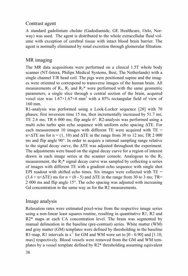
tion in order to cover most clinically relevant concentration levels. First, concentration curves CB(t), CGM(t) and CWM(t) corresponding to arterial input function and tissue response functions were calculated. The AIF CB(t) was defined by a gamma variate function

( ) ∙ / (40)

using a=3 and b =1.5. The resulting AIF was normalized to the peak concen-trations given in Table 1. The tissue response curves were obtained by con-volving CB(t) with an exponential residue function ( ) ∙ / (41)

Perfusion values for GM/WM were set to FB = 60/30 ml/100 ml/min, VB = 4/2 ml/100 ml and tm = 4/4 s. The concentration-time curves were then con-verted into signal intensity curves S(t) by Eq. (26) and Eq. (32) and the re-laxivities presented in Table 2 for the MR sequence parameters and peak concentrations given in Table 1. These S(t) curves, corresponding to ac-quired perfusion data were then translated into corresponding ΔRε(t) curves by applying the normal assumptions regarding negligible secondary relaxa-tion effects previously described. For each type of sequence weighting there were three sets of response curves; the actual concentration curves ΔC(t), the apparent ΔRapp(t) influenced by secondary relaxation effects and the ideally measured ΔRideal(t) not biased by secondary relaxation effects, but influenced by possible blood/tissue relaxation differences. These sets of data were then analyzed using Eq. (11), (13) and (10) to produce the parameters FB, VB and tm and error in the estimates of the three parameters relative to their true val-ues was estimated. In the deconvolution process needed to extract the resi-due function a truncated SVD algorithm was used [17] with two different threshold values: 0.002 and 0.2.

Table 1. Simulation parameters for each MR sequence weighting

T1 T2 T2*

TE (ms) 1.4 100 30TR (ms) 3.8 1 600 1 600Flip angle (°) 13 90 90Peak CB (mM) 3 & 6 6 & 12 6 & 12

41

Statistical analysis Non-parametric independent samples test was used to test for differences in relaxivity between blood, GM and WM for each of the three relaxivity pa-rameters. This test was perfumed both for blood concentration and estimated tissue concentration relaxivities. Differences between blood volume esti-mates based on the three relaxivity parameters was tested for GM and WM, as were differences in tissue blood volume quotient of GM to WM. Differ-ences with p<0.05 were considered statistically significant.

42

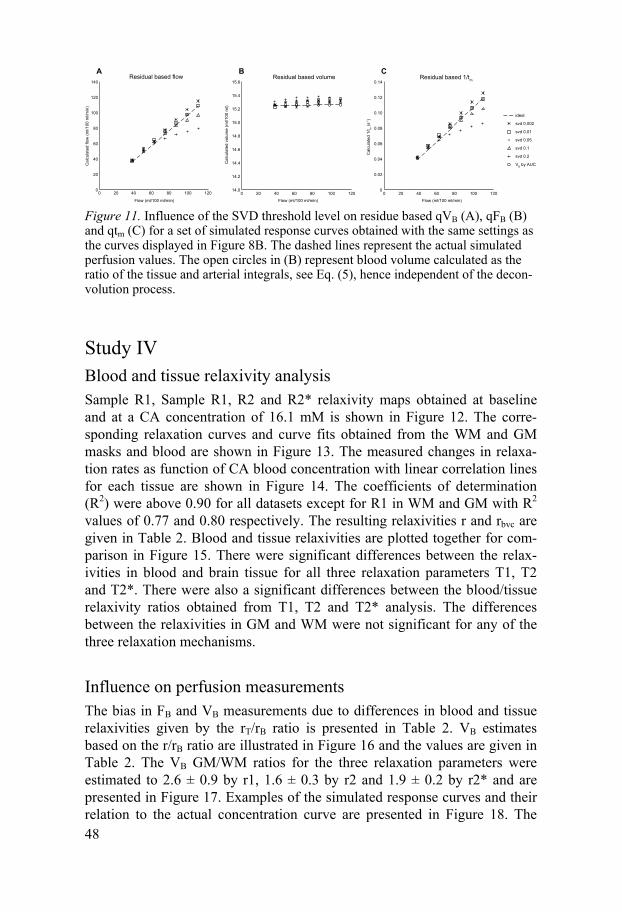
Results

Study I Renal perfusion parameters could be determined in 6 out of 10 patients. Three patients were excluded due to AIF saturation and one was excluded due to technical problems – substantial signal intensity oscillation through-out the data set.

Examples of resulting FB, VB and tm maps are shown in Figure 4. The mean values for cortical FB, VB and tm in the normal kidneys were measured to 339 ± 60 ml/min/100g, 41 ± 8 ml/100g and 7.3 ± 1.0 s respectively, all based on double echo data.

Using single echo instead of double echo data gave on average 25% lower cortical flow values compared to the double echo approach, illustrated in Figure 5.

Figure 4. Examples of regional perfusion maps generated using double echo data; (a) blood flow, (b) blood volume and (c) mean transit time.

43

Figure 5. Illustration of the results acquired using double echo (white) and single echo (grey) data.

Study II Feasibility and general findings Twelve pigs were successfully prepared and connected to CPB, eleven of which were included for further analysis. One pig was excluded because of SVC obstruction with pronounced venous congestion and undetectable cere-bral circulation obvious already at the first SACP levels.

Physiology and blood gas analysis The initial SACP flow was 290±23 ml/min (8ml/kg/min) in group 1 and 230±21 ml/min (6ml/kg/min) in group 2. The SvO2 decreased with reduced flow in group 1 with and significant difference between groups (-44±17% vs. -4±1%; p=0.001) at 2 ml/kg/min, see Figure 6F. The PO2 and SaO2 was normal or supranormal in all cases and flow levels while the pH, BE (base excess), pCO2 and Hct decreased in both groups from the start of CPB until the end of the experiment. No significant differ-ences were seen between groups. Similarly, the mean arterial pressure did not differ between the groups, see Figure 6E.

Metabolic changes Lactate Blood lactate concentrations in arterial blood increased through the experi-ment without significant difference between the groups, see Figure 6B. The retrieved MRS lactate peaks appeared as double peaks at 1.3 ppm as ex-

0

100

200

300

400

500

600

H1 H2 O1 U1 U2 U3Patient ID

Mea

n co

rtica

l blo

od fl

ow [m

l / m

in /

100g

]

44

pected. These peaks were normalized to the concomitant creatine peak at 3 ppm, generally considered constant over time in repeated spectra. At 2 ml/kg/min, the lactate to creatine ratio had increased significantly in group 1 compared with group 2 (167±76% vs. 38±12%; p<0.05), see Figure 6A.

Figure 6. Diagrams describing data collected during the experiment for group 1 (□) and group 2 (■), last data set at 8 ml/kg/min dashed grey. * = P<0.05.

Analysis of cerebral injury Diffusion-weighted imaging (DWI) Technically adequate ADC maps were obtained from each animal and scan-ning panel. No pig displayed regional changes indicative of focal ischemic injury. The regional analysis of the mean ADC in the basal ganglia, neocor-tex and entire hemispheres showed no difference between the groups.

Protein S100β The possible ischemic effects on protein S100β concentrations were assumed to appear less rapidly than venous saturation and lactate changes, and conse-quently, the last flow step of 8 ml/kg/min was included in the between-group comparison in order to detect effects on the 2 ml/kg/min level. No significant difference was present at baseline. A subtle tendency towards higher levels in group 1 could be seen at the start of SACP, however the values were close to baseline and no significant difference was seen between groups. At the flow level of 2 ml/kg/min, a marked increase in mean protein S100β levels was observed in group 1 but not in group 2, and after the return to 8 ml/kg/min, there was a statistically significant difference (115±66% vs.-35±26%; p<0.05) between groups Figure 6C.

Mean relative lactate creatine ratio Mean blood lactate

Blo

od la

ctat

e (m

mol

/L)

Mean relative S100β

Mean relative MTT of whole brain Mean arterial pressure Mean SvO2

Flow (ml/kg/min)

Rel

lact

ate/

crea

tine

ratio

Flow (ml/kg/min)

Flow (ml/kg/min) Flow (ml/kg/min)

Flow (ml/kg/min) Flow (ml/kg/min)

Rel

S10

0β (u

g/L)

Rel

MTT

MA

P (m

mH

g)

SvO

2 (%

)

4

468

3

2

2

*

8

1

0

4

3

2

1

0468 2 8

4

3

2

1

0

15

10

5

0

100

80

60

40

120

100

80

40

60

20

468 2 8

468 2 8 468 2 8

468Base 2 8

A B C

D E F

*

*

45

Perfusion Perfusion-weighted imaging The MTT maps were analyzed and showed globally increasing transit times in response to the stepwise reduced flow rate in group 1 Figure 6D. Relative to the flow of 8 ml/kg/min, the increase in global MTT was 26%±6%, 81%±38% and 220%±167% at flow levels 6, 4 and 2 ml/kg/min, respective-ly. On return to 8 ml/kg/min, MTT recovered accordingly. In group 2, the MTT was slightly prolonged at each step of the experiment, and at the last time point, the observed change reached +50±29% relative to baseline. Lat-eral perfusion asymmetry, defined as a hemispherical difference in CBF of 30% or more, was discovered in 12 of the total 55 perfusion scans and dis-tributed among five subjects; three in group 1 and two in group 2. Of the three subjects in group 1 with CBF asymmetry, occurrence of CBF asym-metry seemed to increase with CBF reduction; 1/6, 0/3, 1/3 and 3/3 at 8 (first and last steps), 6, 4 and 2 ml/kg/min respectively.

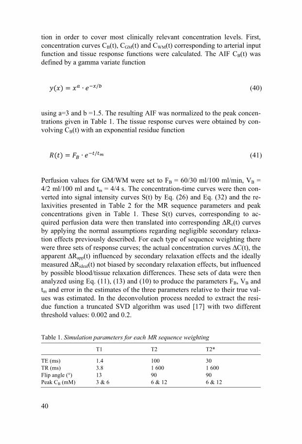
Study III Examples of calculated perfusion maps are given in Figure 7 where pixel-wise distributions of FB, VB and tm are given for the three CPB flow levels for one subject. In Figure 8 AIF and tissue response curves for the same subject are illustrated together with corresponding simulated curves. The behaviour of the quantitative and relative perfusion measurements as whole brain mean values are given in Figure 9 and Figure 10 respectively. For the experimental quantitative FB values the difference between the flow group and control group was not statistically significant. The mean slope for nor-malized qFB by CPB flow was 0.8±0.4 compared to expected 1 for ideal measurements, i.e. a change in FCPB of 100% resulted in a change in FB measured by DSC-MRI of 80%. The influence of the deconvolution regular-ization parameter was substantial for qFB based on noise free simulated data which is illustrated in Figure 11. As the regularization parameter was in-creased from 0.002 to 0.2 the calculated flow decreased by up to 25%, the underestimation being greater for higher flow levels. The simulated data agree fairly well with the experimental data, see Figure 9 and Figure 10.

46

Figure 7. Examples of perfusion maps calculated with the arterial input function for the three CPB flow levels 4, 6 and 8 ml/kg/min. Top row tissue blood flow, middle row tissue blood volume and bottom row mean transit time. CPB flow level increas-es from left to right.

Figure 8. Examples of experimental and simulated response curves for three global flow levels. (A) Experimental curves from subject F5. Arterial response was correct-ed with the venous signal and gamma variate fitted. The tissue curves from a ROI placed in a region with few visible large vessels. (B) Simulated curves for arterial and tissue response.

0

5

10

15

20

0 20 40 60 80 100 120 140 160 180

Sim

ulat

ed c

once

ntra

tion

(ml-1

)

Time (s)

Simulated signals

0

20

40

60

80

100

120

140

160

180

200

0 20 40 60 80 100 120

dR2*

(s-1)

Time (s)

Example experimental signals

4 ml/kg/min 6 ml/kg/min 8 ml/kg/min

A B

47

Figure 9. Quantitative perfusion results for whole brain based on experimental and simulated data. Top row (A, B, C) displays the results of the individual measure-ments in the order of acquisition – FCPB adjusted from 8 to 6 and 4 ml/kg/min. Data points for the flow group are connected with dashed lines and the control group with solid lines. Bottom row (D, E, F) displays normalized mean values ± one standard deviation of the flow group by FCPB together with two sets of corresponding simulat-ed values calculated with different SVD threshold values, 0.002 and 0.2. The solid lines represent ideal 1:1 linear relationship with FCPB and constant volume. The values were normalized to the mean value of the first acquired experimental data point with CPB flow level 8 ml/kg/min.

Figure 10. Relative perfusion results for whole brain based on experimental and simulated data. Top row (A, B, C) displays the results of the individual measure-ments in the order of acquisition – FCPB adjusted to 8, 6 and 4 ml/kg/min. Data points for the flow group are connected with dashed lines and the control group with solid lines. Bottom row (D, E, F) displays normalized mean values ± one standard deviation of the flow group by FCPB together with corresponding simulated values. From left to right rFB, rVB and rtm. The solid line in (F) represent ideal 1:1 linear relationship with FCPB and constant volume. Since tm is inversely proportional to flow 1/tm was plotted against flow in (F). The values were normalized to the mean value of the first acquired experimental data point, CPB flow level 8 ml/kg/min.

0

20

40

60

80

100

120

0 1 2 3

qFB (m

l/min

/100

g)

Measurement

qFB(n)

0

2

4

6

8

10

12

14

0 1 2 3

qtm (s

)

Measurement

qtm(n)

F1

F2

F3

F4

F5

C1

C2

0

20

40

60

80

100

120

140

0 2 4 6 8 10

nqF B

(au)

CPB flow (ml/kg/min)

nqFB(FCPB)

0

2

4

6

8

10

12

0 1 2 3

qVB (m

l/100

g)

Measurement

qVB(n)

0

20

40

60

80

100

120

0 2 4 6 8 10

nqV

B (a

u)

CPB flow (ml/min/kg)

nqVB(FCPB)

0

20

40

60

80

100

120

0 2 4 6 8 10

n(1/

qtm) (

au)

CPB flow (ml/min/kg)

n(1/qtm)(FCPB)

exp

sim svd 0.002

ideal

sim svd 0.2

A B C

D E F

0

5

10

15

20

25

0 1 2 3

rFB (a

u)

Measurement

rFB(n)

0

100

200

300

400

500

600

0 1 2 3

rVB (a

u)

Measurement

rVB(n)

0

5

10

15

20

25

30

0 1 2 3

rt m (a

u)

Measurement

rtm(n)

F1

F2

F3

F4

F5

C1

C2

0

20

40

60

80

100

120

0 2 4 6 8 10

n(1/

rFB) (

au)

CPB flow (ml/kg/min)

n(1/rFB)(FCPB)

0

20

40

60

80

100

120

0 2 4 6 8 10

n(1/

rVB) (

au)

CPB flow (ml/kg/min)

n(1/rVB)(FCPB)

0

20

40

60

80

100

120

0 2 4 6 8 10

n(1/

rt m) (

au)

CPB flow (ml/kg/min)

n(1/rtm)(FCPB)

exp

sim

ideal

A B C

D E F

48

Figure 11. Influence of the SVD threshold level on residue based qVB (A), qFB (B) and qtm (C) for a set of simulated response curves obtained with the same settings as the curves displayed in Figure 8B. The dashed lines represent the actual simulated perfusion values. The open circles in (B) represent blood volume calculated as the ratio of the tissue and arterial integrals, see Eq. (5), hence independent of the decon-volution process.

Study IV Blood and tissue relaxivity analysis Sample R1, Sample R1, R2 and R2* relaxivity maps obtained at baseline and at a CA concentration of 16.1 mM is shown in Figure 12. The corre-sponding relaxation curves and curve fits obtained from the WM and GM masks and blood are shown in Figure 13. The measured changes in relaxa-tion rates as function of CA blood concentration with linear correlation lines for each tissue are shown in Figure 14. The coefficients of determination (R2) were above 0.90 for all datasets except for R1 in WM and GM with R2 values of 0.77 and 0.80 respectively. The resulting relaxivities r and rbvc are given in Table 2. Blood and tissue relaxivities are plotted together for com-parison in Figure 15. There were significant differences between the relax-ivities in blood and brain tissue for all three relaxation parameters T1, T2 and T2*. There were also a significant differences between the blood/tissue relaxivity ratios obtained from T1, T2 and T2* analysis. The differences between the relaxivities in GM and WM were not significant for any of the three relaxation mechanisms.

Influence on perfusion measurements The bias in FB and VB measurements due to differences in blood and tissue relaxivities given by the rT/rB ratio is presented in Table 2. VB estimates based on the r/rB ratio are illustrated in Figure 16 and the values are given in Table 2. The VB GM/WM ratios for the three relaxation parameters were estimated to 2.6 ± 0.9 by r1, 1.6 ± 0.3 by r2 and 1.9 ± 0.2 by r2* and are presented in Figure 17. Examples of the simulated response curves and their relation to the actual concentration curve are presented in Figure 18. The

0

20

40

60

80

100

120

140

0 20 40 60 80 100 120

Cal

cula

ted

flow

(ml/1

00 m

l/min

)

Flow (ml/100 ml/min)

Residual based flow

14.0

14.2

14.4

14.6

14.8

15.0

15.2

15.4

15.6

0 20 40 60 80 100 120

Cal

cula

ted

volu

me

(ml/1

00 m

l)

Flow (ml/100 ml/min)

Residual based volume

ideal

svd 0.002

svd 0.01

svd 0.05

svd 0.1

svd 0.2

VB by AUC

0

0.02

0.04

0.06

0.08

0.10

0.12

0.14

0 20 40 60 80 100 120

Cal

cula

ted

1/t m

(s-1)

Flow (ml/100 ml/min)

Residual based 1/tm A B C

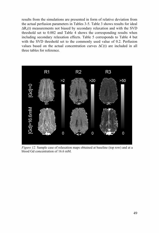
49

results from the simulations are presented in form of relative deviation from the actual perfusion parameters in Tables 3-5. Table 3 shows results for ideal ΔRε(t) measurements not biased by secondary relaxation and with the SVD threshold set to 0.002 and Table 4 shows the corresponding results when including secondary relaxation effects. Table 5 corresponds to Table 4 but with the SVD threshold set to the commonly used value of 0.2. Perfusion values based on the actual concentration curves ΔC(t) are included in all three tables for reference.

Figure 12. Sample case of relaxation maps obtained at baseline (top row) and at a blood Gd concentration of 16.6 mM.

50

Figure 13. Sample brain relaxation curves for T1-relaxation (A), T2-relaxation (C) and T2*-relaxation (D) with corresponding curve fits obtained at [Gd] = 16.6 mM. The curves were generated from the white- and grey matter masks shown in (B).

Figure 14. Measured relaxation rates plotted for blood, GM and WM together with lines representing the corresponding relaxivities. From right to left R1, R2 and R2* for all three tissues in the top row (A, B, C) and corresponding plots for GM and WM in bottom row (D, E, F). No R1 values for blood could be extracted from sam-pled data for concentrations exceeding approximately 15 mM. The line for blood relaxivity in (A) appears biased compared to the data points, this is due to that the line is constructed as the mean slope of all subjects and not a linear fit to all data points pooled together.

-80

-60

-40

-20

0

20

40

60

80

0 500 1000 1500 2000 2500 3000 3500

Sig

nal i

nten

sity

(au)

S

igna

l int

ensi

ty (a

u)

Sig

nal i

nten

sity

(au)

Inversion time (ms)

C

A

0

50

100

150

200

250

300

0 20 40 60 80 100

Echo time (ms)

WM

WM (fit) GM

0

20

40

60

80

100

120

0 10 20 30 40 50 60

Echo time (ms)

GM fit

D

B

0

10

20

30

40

0 5 10 15 20 25 30 35

dR1

(s-1)

dCblood(mM)

dR1(Cblood) for blood, GM and WM A B C

D E F

GM WM Blood

0

0.1

0.2

0.3

0.4

0 5 10 15 20 25 30 35

dR1

(s-1)

dCblood(mM)

dR1(Cblood) for GM and WM Lin GM Lin WM

0

40

80

120

160

0 5 10 15 20 25 30 35

dR2

(s-1)

dCblood(mM)

dR2(Cblood) for blood, GM and WM

Lin blood

0

1

2

3

0 5 10 15 20 25 30 35

dR1

(s-1)

dCblood(mM)

dR2(Cblood) for GM and WM

00

100

200

300

400

5 10 15 20 25 30 35

dR2*

(s-1)

dCblood(mM)

dR2*(Cblood) for blood, GM and WM

-10

0

10

20

30

40

50

60

0 5 10 15 20 25 30 35

dR2*

(s-1)

dCblood(mM)

dR2*(Cblood) for GM and WM

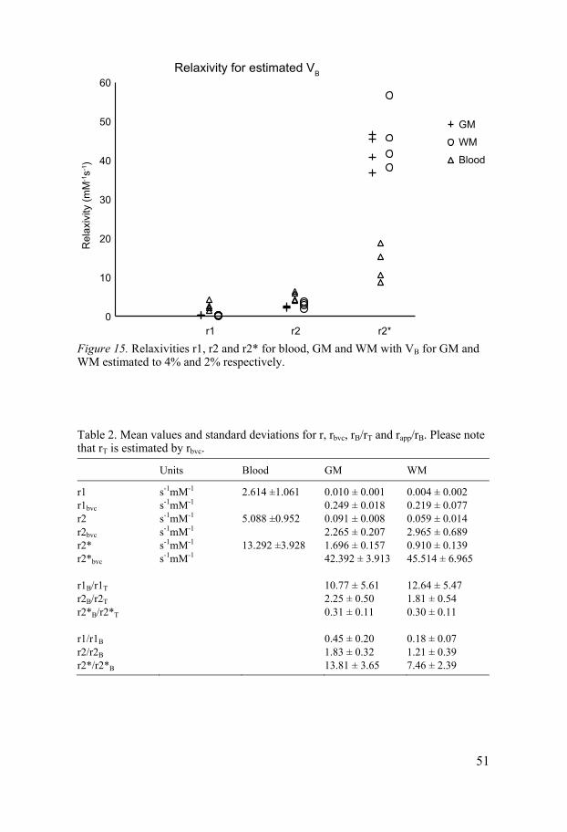
51

Figure 15. Relaxivities r1, r2 and r2* for blood, GM and WM with VB for GM and WM estimated to 4% and 2% respectively.

Table 2. Mean values and standard deviations for r, rbvc, rB/rT and rapp/rB. Please note that rT is estimated by rbvc.

Units Blood GM WM

r1 s-1mM-1 2.614 ±1.061 0.010 ± 0.001 0.004 ± 0.002 r1bvc s-1mM-1 0.249 ± 0.018 0.219 ± 0.077 r2 s-1mM-1 5.088 ±0.952 0.091 ± 0.008 0.059 ± 0.014 r2bvc s-1mM-1 2.265 ± 0.207 2.965 ± 0.689 r2* s-1mM-1 13.292 ±3.928 1.696 ± 0.157 0.910 ± 0.139 r2*bvc s-1mM-1 42.392 ± 3.913 45.514 ± 6.965 r1B/r1T 10.77 ± 5.61 12.64 ± 5.47 r2B/r2T 2.25 ± 0.50 1.81 ± 0.54 r2*B/r2*T 0.31 ± 0.11 0.30 ± 0.11 r1/r1B 0.45 ± 0.20 0.18 ± 0.07 r2/r2B 1.83 ± 0.32 1.21 ± 0.39 r2*/r2*B 13.81 ± 3.65 7.46 ± 2.39

0

10

20

30

40

50

60 R

elax

ivity

(mM

-1s-1

)

r1 r2 r2*

Relaxivity for estimated VB

GM

WM

Blood

52

Figure 16. Tissue blood volume fraction estimates based on the r/rB ratio for GM and WM for the three relaxation parameters.

Figure 17. GM to WM ratio of tissue blood volume for the three relaxivity parame-ters.

0

4

8

12

16

20

r1 r2 r2*

Tiss

ue V

B (%

)

Relaxivity parameter

VB estimates by tissue relaxivity

GM

WM

0

1

2

3

4

r1 r2 r2*

VB G

M to

WM

ratio

Relaxivity parameter

VB GM to WM ratio

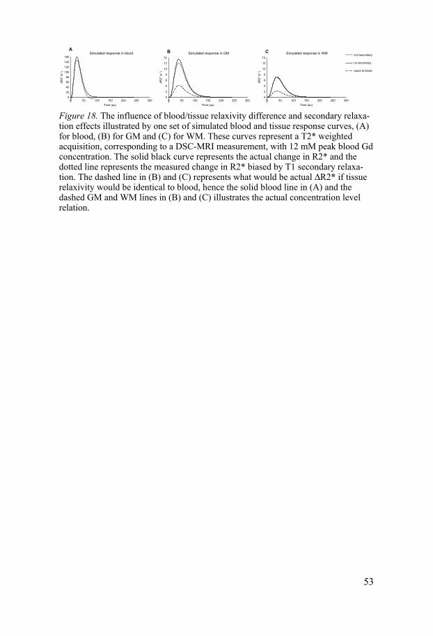
53

Figure 18. The influence of blood/tissue relaxivity difference and secondary relaxa-tion effects illustrated by one set of simulated blood and tissue response curves, (A) for blood, (B) for GM and (C) for WM. These curves represent a T2* weighted acquisition, corresponding to a DSC-MRI measurement, with 12 mM peak blood Gd concentration. The solid black curve represents the actual change in R2* and the dotted line represents the measured change in R2* biased by T1 secondary relaxa-tion. The dashed line in (B) and (C) represents what would be actual ΔR2* if tissue relaxivity would be identical to blood, hence the solid blood line in (A) and the dashed GM and WM lines in (B) and (C) illustrates the actual concentration level relation.

0

20

40

60

80

100

120

140

160

0 50 100 150 200 250 300

dR2*

(s-1)

Time (au)

Simulated response in blood A B C

0

2

4

6

8

10

12

14

0 50 100 150 200 250 300

dR2*

(s-1)

Time (au)

Simulated response in GM

0

2

4

6

8

10

12

14

0 50 100 150 200 250 300

dR2*

(s-1)

Time (au)

Simulated response in WM incl secondary

no secondary

equal to blood

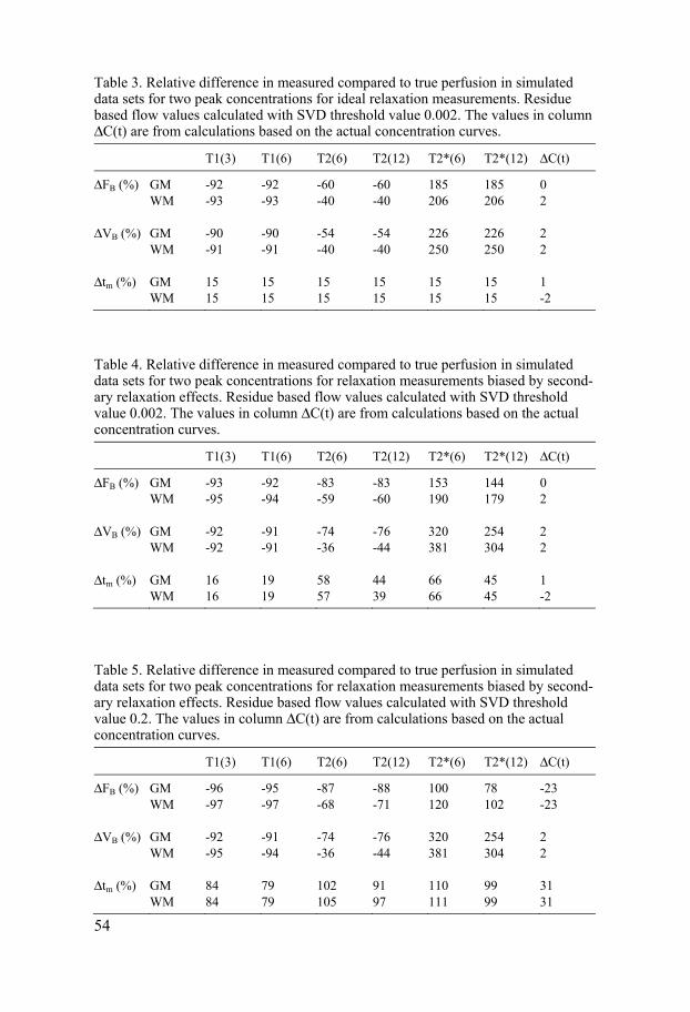
54

Table 3. Relative difference in measured compared to true perfusion in simulated data sets for two peak concentrations for ideal relaxation measurements. Residue based flow values calculated with SVD threshold value 0.002. The values in column ΔC(t) are from calculations based on the actual concentration curves.

T1(3) T1(6) T2(6) T2(12) T2*(6) T2*(12) ΔC(t)

ΔFB (%) GM -92 -92 -60 -60 185 185 0 WM -93 -93 -40 -40 206 206 2 ΔVB (%) GM -90 -90 -54 -54 226 226 2 WM -91 -91 -40 -40 250 250 2 Δtm (%) GM 15 15 15 15 15 15 1 WM 15 15 15 15 15 15 -2

Table 4. Relative difference in measured compared to true perfusion in simulated data sets for two peak concentrations for relaxation measurements biased by second-ary relaxation effects. Residue based flow values calculated with SVD threshold value 0.002. The values in column ΔC(t) are from calculations based on the actual concentration curves.

T1(3) T1(6) T2(6) T2(12) T2*(6) T2*(12) ΔC(t)

ΔFB (%) GM -93 -92 -83 -83 153 144 0 WM -95 -94 -59 -60 190 179 2 ΔVB (%) GM -92 -91 -74 -76 320 254 2 WM -92 -91 -36 -44 381 304 2 Δtm (%) GM 16 19 58 44 66 45 1 WM 16 19 57 39 66 45 -2

Table 5. Relative difference in measured compared to true perfusion in simulated data sets for two peak concentrations for relaxation measurements biased by second-ary relaxation effects. Residue based flow values calculated with SVD threshold value 0.2. The values in column ΔC(t) are from calculations based on the actual concentration curves.

T1(3) T1(6) T2(6) T2(12) T2*(6) T2*(12) ΔC(t)

ΔFB (%) GM -96 -95 -87 -88 100 78 -23 WM -97 -97 -68 -71 120 102 -23 ΔVB (%) GM -92 -91 -74 -76 320 254 2 WM -95 -94 -36 -44 381 304 2 Δtm (%) GM 84 79 102 91 110 99 31 WM 84 79 105 97 111 99 31

55

Discussion

Tissue perfusion assessment by DSC-MRI is in many clinics standard-issue among the battery of clinical MR procedures available. The image acquisi-tion is fairly straight forward and can be performed at any clinical MR scan-ner and for tracer particles the usual gadolinium contrast agents are used. Regarding data analysis there are commercial products enabling fast calcula-tion of perfusion maps in formats compatible with the clinical presentation and archiving systems. The colorful parametric maps displaying the pixel wise distribution of tissue perfusion properties are in many ways very intui-tive for the radiologist, and actually quite beautiful compared to much of the otherwise grey scale dominated material at the radiological departments. In addition, DSC-MRI is often labeled as a quantitative method which yield results in absolute units. However, as illustrated in the studies included in this thesis, there are issues to consider and these also apply to variants of the method in which the response curves are based on change in T1 or T2 in-stead of T2*. The kinetic model, described in the Introduction, can provide accurate absolute flow values but only if the response curves represent the true tracer particle concentration. From a causality point of view, the events following after an intravenous injection of a dose of MR contrast agent into a system with given perfusion properties are described by

, , → ∆ ( ) → ∆ ( ) → ∆ ( ) (42)

The actual tracer particle concentration variation over time in a specific vol-ume of tissue will cause corresponding variations in blood and tissue relaxa-tion properties which in turn causes signal intensity variations in the ac-quired MR images. From the observer’s point of view, the task is to follow this chain of events the other way, and hopefully arrive at a set of parameters truthfully reflecting the perfusion properties of the tissue of interest; ∆ ( ) → ∆ ( ) → ∆ ( ) → , , (43)

56

The first task is to transform the recorded variation in MR image signal in-tensity into the underlying change in relaxation rate. The second is to esti-mate the actual variation in contrast agent concentration based on the as-sessed variation in relaxation rate. The third step is to by use of the indicator dilution model translate the calculated arterial and tissue concentration curves into hemodynamic parameters.

The studies included in this thesis cover sources of error associated with these three steps and how the calculated hemodynamic variables are influ-enced by choice of measurement technique, assumptions and calculation process variables.

From signal intensity to relaxation rate Contrast agents have mixed relaxation effects, and what effect will dominate depends on concentration level and choice of MR sequence parameters, typi-cally TE, TR and flip angle. Image data collected with conventional MR sequences, i.e. single echo acquisitions, is inherently more or less susceptible to secondary relaxation.

For the iron oxide based contrast agent used in study I, the influence of secondary T1 relaxation on DSC-MRI perfusion values were substantial leading to underestimations of tissue blood flow and volume in the order of 30% as estimated by single/double echo data. Corresponding effect for the gadolinium based contrast agent in study IV was estimated to about 10% from numerical simulations based on the measured in vivo relaxivity values. In another study the effect was estimated to an underestimation of 40% [34].

From relaxation rate to concentration In order to translate the (estimated) variation in relaxation rate into underly-ing variation in tracer particle concentration it is normally assumed that the contrast agent relaxivities in blood and tissue are identical and linear. In study IV the in vivo T1, T2 and T2* relaxivities for a clinically used gado-linium based contrast agent (Gadodiamide, GE Healthcare, Oslo, Norway) were measured in blood and cerebral tissue in pig. While the acquired data showed linear relaxation rate dependence for all three relaxation mechanisms the differences between blood and cerebral tissue relaxivity were substantial. The measured values for r2* for blood and cerebral tissue agree well with previously published values based on ex vivo measurements [35] and numer-ical simulations [15], see Figure 19.

The influence of observed blood/tissue relaxivity differences on DSC-MRI measurements was assessed by tissue to blood relaxation ratios and

57

numerical simulations of response curves to approximately three-fold over-estimations for blood flow and volume. In a study by Jochimsen et al [36] regarding systematic errors in DSC-MRI a four-fold overestimation of blood flow and volume was attributed to differences in blood and tissue relaxivi-ties.

From concentration curves to blood flow and volume The principles of the indicator dilution model is independent of choice of modality and for ideal computation processes the accuracy of the calculated hemodynamic parameters is only limited by the precision of the input con-centration curves. Numerical simulations in study III and IV based on “per-fect” noise free data indicated that the SVD threshold level have a substan-tial effect on the blood flow values. The bias introduced by the SVD thresh-old displayed a distinct flow level dependency – the underestimating effect was markedly stronger for increasing flow levels, see Figure 11. This behav-ior indicates that the bias due to the SVD threshold is not only an issue re-garding the overall accuracy or potential for truly quantitative perfusion measurements by DSC-MRI but also for the clinically common intra-subject comparisons between different regions. One should be aware of the risk that the measured flow in regions with high flow will be underestimated relative to regions with lower flow.

Arterial input function properties Besides the influence of tissue/blood relaxivity differences, secondary relax-ation and SVD threshold level covered in studies I, III and IV there are sev-eral other sources of error that should be considered. By inspection of Eq. (11) and Eq. (14) in the Introduction section it is evident that the precision of the AIF is crucial. Critical issues are saturation and partial volume effects but also bolus delay and dispersion [20, 21, 37, 38]. Delay regards the timing difference between the AIF and the tissue response and there are established methods to account for this effect which otherwise may lead to significant errors. Dispersion regards the modulation of the arterial bolus during transport from the AIF sampling site to the tissue. Since the effect depends on the structure and flow properties of the vascular tree between the two sampling sites, a correction strategy for dispersion is a complicated matter

Perfusion estimation without arterial input function The basic prerequisites for DSC-MRI are essentially a sampled arterial input function and corresponding tissue responses. Considering the dependence of

58

the quality of the AIF it would be of interest if some perfusion properties could be extracted from the tissue response only. From a signal analysis point of view the tissue response appear more stable than the corresponding AIF, although with lower dynamic range. A tissue region of interest would typically consist of tens to hundreds of pixels effectively averaging out much of the noise inherent to the rapid imaging techniques needed for the high temporal resolution. Directly related to the temporal resolution is the number of sampling points available to define the arterial and tissue curves. The AIF, being both shorter and higher, is more susceptible for erroneous estimation of its true shape and true peak amplitude than the slower tissue response having a more favorable temporal width compared to the sampling rate. In study II, in which repeated perfusion acquisitions were made at different total flow levels in a number of pigs, it proved impossible to obtain repro-ducible arterial input functions in all subjects. A relative measure of tm was used instead, based exclusively on the tissue response; ( )( ) (44)

This relation seemed to reflect the expected changes in global flow level in a reasonable manner during the analysis in study II. In study III, the mean transit time was calculated with and without AIF deconvolution. By inspec-tion of the results illustrated in Figure 9F and Figure 10F it seems that the relative measure actually agrees to a slightly higher degree with the ideal response to a change in global flow level. However, the good agreement may be incidental and due to favorable relations between the width of the AIF and the tissue perfusion properties following from the specific experimental setup. There are several alternative perfusion parameters, in the sense being acquired without using an AIF, and in a study by Perthen et al [39] a number of these, such as full width at half maximum and time to peak, were studied. Their conclusion was that these parameters must be used with caution since none of the parameters tested were independent of the AIF. However, con-sidering the challenges associated with first acquiring a correct AIF and then deconvolving it successfully from the tissue response it may seem tempting to further investigate the potential of perfusion analysis based on tissue re-sponse curves alone.

59

Figure 19. Comparison of experimental results for r2* in blood and tissue with pre-viously published data; in vitro blood curve from van Osch [35] (dashed) and simu-lated cerebral tissue from Kjølby [15] (solid). Experimental curves for blood (solid), GM (dotted) and WM (dot-dashed). Estimated tissue blood volume fractions, in order to obtain blood volume corrected relaxivities, were 4% for GM and 2% for WM.

0

100

200

300

400

500

600

700

800

0 5 10 15 20

dR2*

(s-1)

Gd concentration (mM)

Comparison to selected published values

Blood van Osch

Blood exp

Tissue Kjølby GM exp

WM exp

60

Conclusions

Perfusion measurements in kidneys by DSC-MRI using an iron oxide based blood pool agent were shown to be feasible. The influence of secondary relaxation effects proved to be substantial leading to underestimation of tis-sue blood flow and volume. It was further demonstrated that the secondary relaxation effect can be corrected for by using a double echo sequence.

Based on careful planning and execution it is possible to monitor the cere-bral perfusion during an experimental cardio pulmonary bypass procedure by MRI. The results indicated an ischemic threshold level at a CPB blood flow rate of approximately 6 ml/kg/min.

Calculations based on experimental- and simulated data supports that DSC-MRI can discriminate between different global flow levels in the same sub-ject given that all other parameters are kept constant. However, the calcula-tions also indicate that the calculated perfusion values are highly sensitive to the specific parameters used during the arterial deconvolution procedure necessary to estimate perfusion from the measured tissue response.

Contrary to the common assumption, the ratio between blood and tissue re-laxivity is not unity and not independent of relaxation mechanism used. For conventional scanning techniques the situation is further complicated by secondary relaxation effects which depend on the sequence parameters, trac-er concentration, type of tissue and tissue blood volume. In T2*-based perfu-sion analysis, using regularization as part of the deconvolution procedure appears to partly counteract the overestimation in perfusion induced by dif-ference in blood/tissue relaxivity.

In general, for contrast agents with an intravascular distribution, DSC-MRI is a versatile method to investigate tissue perfusion related parameters, providing estimates of regional distributions of tissue blood flow and vol-ume. However, the fundamental assumption of equal blood and tissue relax-ivity is experimentally shown to be invalid and the influence of this discrep-ancy substantial. There are several other factors contributing to measurement errors including secondary relaxation and choice of deconvolution parame-ters, both addressed in the present work, and several other factors previously

61

addressed by others. A combination of these factors can incidentally lead to additive errors or error cancellation based on a variety of experimental and analysis conditions. However, given that the substantial differences in blood/tissue relaxivity cannot readily be accounted for in a clinical setting, absolute perfusion quantification by tracer based MRI remains challenging if not impossible.

62

Acknowledgements

Main supervisor professor Atle Bjørnerud, for sharing your understanding of MRI and its applications, having an open mind for all questions and ideas and your kind way. I really enjoyed the discussions during my visits to Oslo and I hope we will continue working together. Supervisor professor Håkan Ahlström, for general guidance regarding scien-tific writing, plenty of scanner hours and a fair amount of gadolinium. Fredrik Lennmyr, Ove Jonsson and Thomas Tovedal, for true teamwork, it has been a pleasure. Fredrik, I trust there is more to come! Gunnar, Stefan and Vitas at the department of Thoracic surgery and Anne, Agneta, Eva-Maria and Karin at the Hedenstierna laboratory for keeping the positive atmosphere during the long experiments. All co-authors for good collaboration. Lars Johansson for sharing your expertise in experimental MRI and Anders Lundberg teaching me to pilot old faithful. Christl Richter-Frohm for help with administrative issues regarding the postgraduate studies and Håkan Pettersson for preparation of all those figures. My colleagues and friends at Medical Physics, especially the radiology group; Karin, Lasse, Malin, Per-Erik and Ragge for the friendly environ-ment. Superiors Lars Jangland and Anders Montelius for prioritizing this project and allowing dedicated time in the final stages, it would never have been completed otherwise. Karin for taking care of the clinical and project support during the research periods and Majsan for keeping Majsans fik al-ways open. Britt-Marie Bolinder, when I came to Uppsala University Hospital almost 10 years ago I had no idea how little I knew about MRI… Thank you for shar-ing your knowledge and experience. Tomas Bjerner, your positive energy is simply outstanding.

63

Colleagues and friends at BFC; Agneta, Ali, Andreas Anne-Marie, Annelie, Carro, Claudia, Elna-Marie, Erik, Eva B, Eva N, Gunilla, Helen, Irfan, Jo-han, Kenneth, Lillemor, Maggan F, Maggan W, Malin, Martin, Per P, Raili, Sara-Lisa, Tomas H et al and colleagues and friends at MIT radiology; Erik, Håkan, Manne, Martin, Niklas, Per, Thomas, and Åke. Small talk and smiles make the world go around. Friends and teammates in URFC, for blood, sweat and beers. My parents Margaretha & Carl Johan and parents-in-law Britt & Kent for all help with babysitting. My wife Eva and my children Tyra, Axel and Elsa. You have been extreme-ly patient and supportive during the final intense months and I look forward to the best summer ever. Yes, the laptop will stay at the office… :-)

64

65

References

1. Belliveau, J.W., et al., Functional cerebral imaging by susceptibility-contrast NMR. Magn Reson Med, 1990. 14(3): p. 538-46.

2. Larson, K.B., et al., Tracer-kinetic analysis for measuring regional cerebral blood flow by dynamic nuclear magnetic resonance imaging. J Theor Biol, 1994. 170(1): p. 1-14.

3. Villringer, A., et al., Dynamic imaging with lanthanide chelates in normal brain: contrast due to magnetic susceptibility effects. Magn Reson Med, 1988. 6(2): p. 164-74.

4. Meier, P. and K.L. Zierler, On the theory of the indicator-dilution method for measurement of blood flow and volume. J Appl Physiol, 1954. 6(12): p. 731-44.

5. Zierler, K.L., Equations for Measuring Blood Flow by External Monitoring of Radioisotopes. Circ Res, 1965. 16: p. 309-21.

6. Purcell, E.M., H.C. Torrey, and R.V. Pound, Resonance absorption by nuclear magnetic moments in a solid. Physical Review, 1946. 69(1-2): p. 2.

7. Bloch, F., Nuclear induction. Physical Review, 1946. 70(7-8): p. 15. 8. Lauterbur, P.C., Image Formation by Induced Local Interactions: Examples

Employing Nuclear Magnetic Resonance. Nature, 1973. 242: p. 2. 9. Lauffer, R.B., Paramagnetic metal complexes as water proton relaxation agents

for NMR imaging: Theory and design. Chemical Review, 1987. 87: p. 27. 10. Caravan, P., et al., Gadolinium(III) Chelates as MRI Contrast Agents: Structure,

Dynamics, and Applications. Chem Rev, 1999. 99(9): p. 2293-352. 11. Freed, J.H., Dynamic effects of pair correlation functions on spin relaxation by

translational diffusion in liquids. II. Finite jumps and independent T1 processes. Journal of Chemical Physics, 1978. 68(9): p. 4.

12. Boxerman, J.L., et al., MR contrast due to intravascular magnetic susceptibility perturbations. Magn Reson Med, 1995. 34(4): p. 555-66.

13. Weisskoff, R.M., et al., Microscopic susceptibility variation and transverse relaxation: theory and experiment. Magn Reson Med, 1994. 31(6): p. 601-10.

14. Frohlich, A.F., L. Ostergaard, and V.G. Kiselev, Theory of susceptibility-induced transverse relaxation in the capillary network in the diffusion narrowing regime. Magn Reson Med, 2005. 53(3): p. 564-73.

15. Kjolby, B.F., L. Ostergaard, and V.G. Kiselev, Theoretical model of intravascular paramagnetic tracers effect on tissue relaxation. Magn Reson Med, 2006. 56(1): p. 187-97.

16. Rempp, K.A., et al., Quantification of regional cerebral blood flow and volume with dynamic susceptibility contrast-enhanced MR imaging. Radiology, 1994. 193(3): p. 637-41.

17. Ostergaard, L., et al., High resolution measurement of cerebral blood flow using intravascular tracer bolus passages. Part I: Mathematical approach and statistical analysis. Magn Reson Med, 1996. 36(5): p. 715-25.

66

18. Calamante, F., D.G. Gadian, and A. Connelly, Quantification of bolus-tracking MRI: Improved characterization of the tissue residue function using Tikhonov regularization. Magn Reson Med, 2003. 50(6): p. 1237-47.

19. Larsson, H.B., et al., Dynamic contrast-enhanced quantitative perfusion measurement of the brain using T1-weighted MRI at 3T. J Magn Reson Imaging, 2008. 27(4): p. 754-62.

20. Wu, O., et al., Effects of tracer arrival time on flow estimates in MR perfusion-weighted imaging. Magn Reson Med, 2003. 50(4): p. 856-64.

21. Wu, O., et al., Tracer arrival timing-insensitive technique for estimating flow in MR perfusion-weighted imaging using singular value decomposition with a block-circulant deconvolution matrix. Magn Reson Med, 2003. 50(1): p. 164-74.

22. Russell, W.M.S. and R.L. Burch, The principles of humane experimental technique1959, London,: Methuen. 238 p.

23. Rydland, J., et al., New intravascular contrast agent applied to dynamic contrast enhanced MR imaging of human breast cancer. Acta Radiol, 2003. 44(3): p. 275-83.

24. Bjornerud, A., L.O. Johansson, and H.K. Ahlstrom, Renal T(*)(2) perfusion using an iron oxide nanoparticle contrast agent--influence of T(1) relaxation on the first-pass response. Magn Reson Med, 2002. 47(2): p. 298-304.

25. Bjornerud, A., et al., Assessment of T1 and T2* effects in vivo and ex vivo using iron oxide nanoparticles in steady state--dependence on blood volume and water exchange. Magn Reson Med, 2002. 47(3): p. 461-71.

26. Jonsson, O., et al., Minimal safe arterial blood flow during selective antegrade cerebral perfusion at 20 degrees centigrade. Ann Thorac Surg, 2011. 91(4): p. 1198-205.

27. Knutsson, L., et al., Absolute quantification of cerebral blood flow in normal volunteers: correlation between Xe-133 SPECT and dynamic susceptibility contrast MRI. J Magn Reson Imaging, 2007. 26(4): p. 913-20.

28. Deichmann, R. and A. Haase, Quantification of T1 values by SNAPSHOT-FLASH NMR imaging. J Magn Reson, 1992. 96: p. 5.

29. Kuppusamy, K., et al., In vivo regional cerebral blood volume: quantitative assessment with 3D T1-weighted pre- and postcontrast MR imaging. Radiology, 1996. 201(1): p. 106-12.

30. Lin, W., A. Celik, and R.P. Paczynski, Regional cerebral blood volume: a comparison of the dynamic imaging and the steady state methods. J Magn Reson Imaging, 1999. 9(1): p. 44-52.

31. Newman, G.C., et al., Cerebral blood volume measurements by T*2-weighted MRI and contrast infusion. Magn Reson Med, 2003. 50(4): p. 844-55.

32. Ito, H., et al., Database of normal human cerebral blood flow, cerebral blood volume, cerebral oxygen extraction fraction and cerebral metabolic rate of oxygen measured by positron emission tomography with 15O-labelled carbon dioxide or water, carbon monoxide and oxygen: a multicentre study in Japan. Eur J Nucl Med Mol Imaging, 2004. 31(5): p. 635-43.

33. Bjornerud, A. and K.E. Emblem, A fully automated method for quantitative cerebral hemodynamic analysis using DSC-MRI. J Cereb Blood Flow Metab, 2010. 30(5): p. 1066-78.

34. Calamante, F., E.J. Vonken, and M.J. van Osch, Contrast agent concentration measurements affecting quantification of bolus-tracking perfusion MRI. Magn Reson Med, 2007. 58(3): p. 544-53.

67

35. van Osch, M.J., et al., Measuring the arterial input function with gradient echo sequences. Magn Reson Med, 2003. 49(6): p. 1067-76.

36. Jochimsen, T.H., et al., Identifying systematic errors in quantitative dynamic-susceptibility contrast perfusion imaging by high-resolution multi-echo parallel EPI. NMR Biomed, 2007. 20(4): p. 429-38.

37. Calamante, F., Bolus dispersion issues related to the quantification of perfusion MRI data. J Magn Reson Imaging, 2005. 22(6): p. 718-22.

38. Calamante, F., D.G. Gadian, and A. Connelly, Delay and dispersion effects in dynamic susceptibility contrast MRI: simulations using singular value decomposition. Magn Reson Med, 2000. 44(3): p. 466-73.

39. Perthen, J.E., et al., Is quantification of bolus tracking MRI reliable without deconvolution? Magn Reson Med, 2002. 47(1): p. 61-7.