Quantitative Standards for Absolute Linguistic...

Cognitive Science (2013) 1–21Copyright © 2013 Cognitive Science Society, Inc. All rights reserved.ISSN: 0364-0213 print / 1551-6709 onlineDOI: 10.1111/cogs.12088

Quantitative Standards for Absolute Linguistic Universals

Steven T. Piantadosi,a Edward Gibsonb

aDepartment of Brain and Cognitive Sciences, University of RochesterbDepartment of Brain and Cognitive Sciences, MIT

Received 10 February 2011; received in revised form 11 October 2012; accepted 4 January 2013

Abstract

Absolute linguistic universals are often justified by cross-linguistic analysis: If all observed lan-

guages exhibit a property, the property is taken to be a likely universal, perhaps specified in the

cognitive or linguistic systems of language learners and users. In many cases, these patterns are

then taken to motivate linguistic theory. Here, we show that cross-linguistic analysis will very

rarely be able to statistically justify absolute, inviolable patterns in language. We formalize two

statistical methods—frequentist and Bayesian—and show that in both it is possible to find strict

linguistic universals, but that the numbers of independent languages necessary to do so is gener-

ally unachievable. This suggests that methods other than typological statistics are necessary to

establish absolute properties of human language, and thus that many of the purported universals in

linguistics have not received sufficient empirical justification.

Keywords: Linguistic universals; Typology; Statistical methods; Statistical model

1. Introduction

One of the primary goals of cognitive science is to characterize the mental representa-

tions and processes that are shared across all humans. Universal features of cognition are

interesting in part because they lead to plausible candidates for genetically encoded repre-

sentations and processes, and in many cases characterize the uniquely human features of

thought. In cognition, universals have been proposed in nearly every domain, ranging

from color naming (Kay & Regier, 2003) to high-level domains such as moral reasoning

(Mikhail, 2007), geometrical intuitions (Dehaene, Izard, Pica, & Spelke, 2006), folk biol-

ogy (Atran et al., 1998), and numerical reasoning (Pica, Lemer, Izard, & Dehaene, 2004),

among others. Perhaps the most well-developed theories of cognitive universals come

from the domain of language typology, which has long attempted to characterize the

Correspondence should be sent to Steven T. Piantadosi, Department of Brain and Cognitive Sciences, Uni-

versity of Rochester, NY 14627. E-mail: [email protected]

range of possible human linguistic systems. An understanding of the breadth—or lack

thereof—of human languages is key for making sense of human thought and communica-

tion. For instance, the science of language should aim to uncover whether all languages

have properties such as recursion, lexical categories, or principles of binding theory.

These types of linguistic features have motivated substantial cognitive theories about the

representations learners bring to acquisition (e.g., Hauser, Chomsky, & Fitch, 2002; Wex-

ler & Culicover, 1983; Wexler & Manzini, 1984, among others). Here, we study the

amount of evidence necessary to make reasonable statistical inferences about such univer-

sals. While we focus on linguistic universals, our methods and general approach are also

applicable to cognitive domains outside of language.

In linguistic typology, core universal representations have long been hypothesized.

Greenberg (1963) described two different classes of universal patterns in languages (for

discussion, see Bickel, 2007a). First, there are violable statistical tendencies, patterns

which hold with higher than chance frequency across language. We refer to these as typi-cality universals.1 An example is Greenberg’s (1963) first universal that subjects tend to

precede objects in simple declarative sentences. This is not true of all the world’s

languages, but it is evidenced in the non-uniform distribution of word orders across

languages. Typology also formalizes absolute constraints, meaning ones which strictly

constrain the space of humanly possible languages. While nearly all instances of absolute

constraints are contested (see Evans & Levinson, 2009), prototypical examples include

the presence of linguistic features such as WH-movement and auxiliaries (Pinker &

Bloom, 1990) or recursion (Hauser et al., 2002). There are also implicational absolutes,

such as Greenberg’s (1963) universal that languages with VSO word order are always

prepositional. Though some have argued that typicality universals are more informative

and useful than absolute ones (Bickel, 2007b; Cysouw, 2005a; Dryer, 1997; Nichols,

1992) or that typological data are not relevant to universal grammar (Haspelmath, 2004;

Newmeyer, 1998, 2004), we believe that the most substantive and interesting theories

about cognition would come from absolute universals. Such universals—if any exist—would delineate necessary properties of human languages and thus characterize hard con-

straints on cognitive capacities. They also provide hypotheses about what knowledge or

constraints humans bring to the problem of language learning—what makes humans dis-

tinctively human.

Statistical methods for typicality universals have been extensively developed and dis-

cussed previously (for an excellent review, see Cysouw, 2005a). A basic challenge with

testing typicality universals is that the set of existing languages may not form a represen-

tative sample in the space of all possible human languages. For instance, if it is observed

that SOV word order is more frequent than OVS, this might be due to chance rather than

biology: Perhaps SOV languages just happened to be the ones that survive to the present

day. However, the problem is more serious than just the effects of random chance. The

processes of language change and contact create languages with correlated features (e.g.,

Dunn, Greenhill, Levinson, & Gray, 2011), meaning that some features will be over-rep-

resented much more than would be expected just by pure random sampling.2 Many

authors have proposed addressing this problem using a sample of languages which is as

2 S. T. Piantadosi, E. Gibson / Cognitive Science (2013)

independent as possible, for instance looking at stratified samples (e.g., Tomlin, 1986),

languages in distinct genera (Dryer, 1989, 1991, 1992), distinct geographical regions

(Dryer, 2000; Maslova, 2000), or with distinct linguistic features (Perkins, 1989; Rijkhof

& Bakker, 1998; Rijkhoff, Bakker, Hengeveld, & Kahrel, 1993). Such statistical tests are

not clearly applicable to absolute universals, since they are designed to compare relative

frequencies, not to determine when the true frequency of a feature is zero.

Indeed, absolute universals provide an interesting puzzle for scientific methodology:

The presence of an absolute constraint can only be inferred from what has not yet been

observed. But, as is often pointed out by typologists, it is always possible that an excep-

tion to a universal constraint might be observed with one additional language (Bell, 1978;

Bickel, 2001; Dryer, 1989). Dryer (1989) describes the problem as

... no matter how many languages we examine and find conforming to an absolute

universal, we can never know that there is not another language that fails to confirm to

the universal, either one that was once spoken or a hypothetical language that is possi-

ble but never actually spoken due to historical accident. What this means is that abso-

lute universals are never testable.3 ... No amount of data conforming to the

generalization provides any reason to believe that there are no languages that do not

conform. And no evidence from attested languages can provide any basis for believing

that exceptions are not possible.

For Dryer, this is both the logical problem of induction, and a statistical puzzle of how

we can know whether features are low probability or zero probability. Bickel (2001) goes

so far as to say that cross-linguistic analysis “cannot in principle contribute” to the dis-

covery of what is possible and impossible in human languages since “a probabilistic

statement is not, and cannot be converted into, a possibility statement.” He recounts

examples of linguistic phenomena that were previously—and erroneously—thought to be

universally impossible, including for instance syntactic ergativity without morphological

ergativity, and pronoun borrowing.

Dryer and Bickel—and before them, Bell—are correct in a strict logical sense:

Observed languages can never conclusively show that an unobserved feature is impossi-

ble. However, the point of this article is to argue that nonetheless, absolute universals are

still valid terrain for inductive scientific inferences. In particular, we develop two methods

for inferring when an absolute constraint is probably true—for when a reasonable induc-

tive scientist should conclude that there is likely to be a cognitive constraint on possible

languages. We first present a method centered around the frequentist idea of keeping a

low false positive rate of proposing linguistic universals. Then, we develop a formal

mathematical model that computes the degree of belief one should have that property of

language is impossible, given a set of sampled languages. We explore the bounds pro-

vided by the formal tools we develop. We will argue that the amount of statistical

evidence required to justify absolute universals will typically be much more than is

achievable with the present set of languages in existence. This is unfortunate for anyone

seeking to justify universals by cross-linguistic comparison. But the real importance of

S. T. Piantadosi, E. Gibson / Cognitive Science (2013) 3

this result is that apparently absolute typological patterns are themselves poor motivations

for linguistic theories. For instance, even if every language in existence exhibited a

feature such as recursion, movement, or auxiliaries, that alone would not be enough to

justify these as cognitively required properties of all possible human languages.

Following Tily and Jaeger (2011), we argue, instead, that other sources of evidence such

as learning experiments are necessary.

This challenge of inferring restrictions based on what is not observed is faced much

more broadly in cognitive and linguistic research. A key example is a classic learnability

problem, the subset problem (Wexler & Manzini, 1984), which holds that learners may

incorrectly hypothesize an under-restrictive linguistic system (e.g., grammar), and never

receive contradictory evidence. For instance, learners might incorrectly guess that certain

types of unobserved and ungrammatical sentences actually are grammatical; if learners

only change hypotheses when they hear counterexamples, their over-generalization will

never be corrected. This problem appears in many areas of language acquisition, includ-

ing syntax (Berwick, 1985; Wexler & Manzini, 1984), phonology (Hale & Reiss, 2003;

Smolensky, 1996), and the learning of compositional sentence structures (Crain, Ni, &

Conway, 1994). Our case is analogous: We want to know whether certain unobserved

features are truly impossible. Like good learners of language, we would like to avoid

both (a) positing necessary restrictions on human language, and (b) missing good general-

izations about what is truly disallowed. Perhaps unsurprisingly, the statistical tools we

use are closely related to statistical models that provide sensible and rational solutions to

the subset problem in language learning (Perfors, Tenenbaum, & Regier, 2011b; Piantad-

osi, Goodman, & Tenenbaum, 2013; Xu & Tenenbaum, 2007).

The outline of this article is as follows: In the next section, we formalize a frequentist

framework for testing absolute universals. After presenting a case study on word order

which demonstrates several important methodological points, we apply a bootstrapping

techniques to 138 features from the World Atlas of Linguistic Structures (Haspelmath,

Dryer, Gil, & Comrie, 2005) and show that incorrect absolutes are often inferred by

drawing fewer than around 500 independently sampled languages. We then present a

Bayesian statistical model for this problem and apply it to studying Greenberg’s Univer-

sal 20 (Cinque, 2005; Cysouw, 2010a; Hawkins, 1983; Rijkhoff, 1990, 1998, 2002), con-

cerning the order of elements in a noun phrase. This example illustrates both the

difficulty of justifying this universal, and ways in which formal modeling can nonetheless

lead to non-trivial findings. In the conclusion, we discuss alternative approaches to dis-

covering universals.

2. Bootstrapping word order

In this article, we focus on making inferences about the absolute constraints on some

observed feature of language F. We suppose that F has N particular values that any

language could exhibit, which exhaust the space of logically possible feature values.4 For

instance, F might be a language’s word order, a language’s preferred linear order of


subject, verb, and object. For word order, there are seven different possible values for

F: SVO, SOV, OSV, OVS, VSO, VOS, and ND (no dominant word order).

Much work in linguistics attempts to find suspicious gaps of feature values that do not

appear in language. Here, we focus on limiting the rate at which we think that observed

gaps are indicative of impossible features. A complementary problem is that of limiting

the number restrictions that are mistakenly thought to be possible (false negatives), but we

do not address that here. In reasoning from observed instances to hypothesized restrictions,

one might incorrectly infer a restriction on features (a false positive error). For instance, if

fewer languages had survived to the present day, we might not have seen a language with

OSV word order, and might have thought that this order was somehow impossible with

human cognitive systems. Our first way of dealing with potential false positives is to con-

trol them—to estimate the rate at which we would falsely posit absolute universals if we

examined a given number of languages. It is impossible to entirely avoid false positives;

instead, we choose a method to keep the false positive probability below a bound, perhaps

0.05, the standard for publication in psychology. This means that 1 in 20 findings of uni-

versal constraints with this method will be false positives. However, for what are essen-

tially non-repeatable experiments (since there are only finitely many languages to test),

one may actually desire a much smaller false positive rate of 0.01 or 0.001.

It is useful to focus on the example of word orders in order to illustrate the logic of our

approach. We can imagine that a naive scientist observed L human languages and posited that

any word orders unobserved in their sample were probably disallowed by cognitive mecha-

nisms. Such a conclusion, we know, would be a false positive error since all seven word orders

actually are allowed. Through simulation (c.f. Haspelmath & Siegmund, 2006) we can deter-

mine what false positive rate this method would give as the number of languages observed,

L, varies. A simple version of this computation was performed by Bell (1978). Ideally, to

compute this, we would assume the scientist sampled L languages from the true distribution of

possible human language.5 However, we do not know the true distribution of word orders.

Instead, we can use a trick known as bootstrapping (see Davison & Hinkley, 1997), where we

approximate the true distribution with the empirically observed distribution. In our case, we

sample word orders from the distribution of word orders in a large database, treating this large

sample as a “good enough” approximation to the real thing. Here, for simplicity, we sample

from the empirically observed distribution in the World Atlas of Linguistic Structures (WALS)

(Dryer, 2005). Importantly, the sampling is done with replacement in order to simulate

sampling from the infinity of possible human languages.

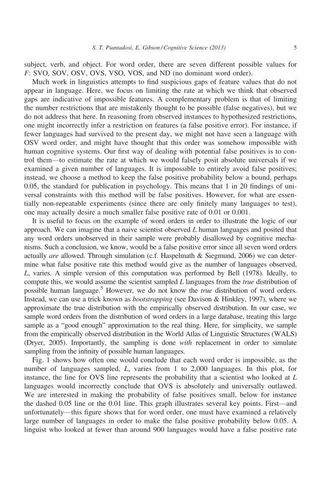
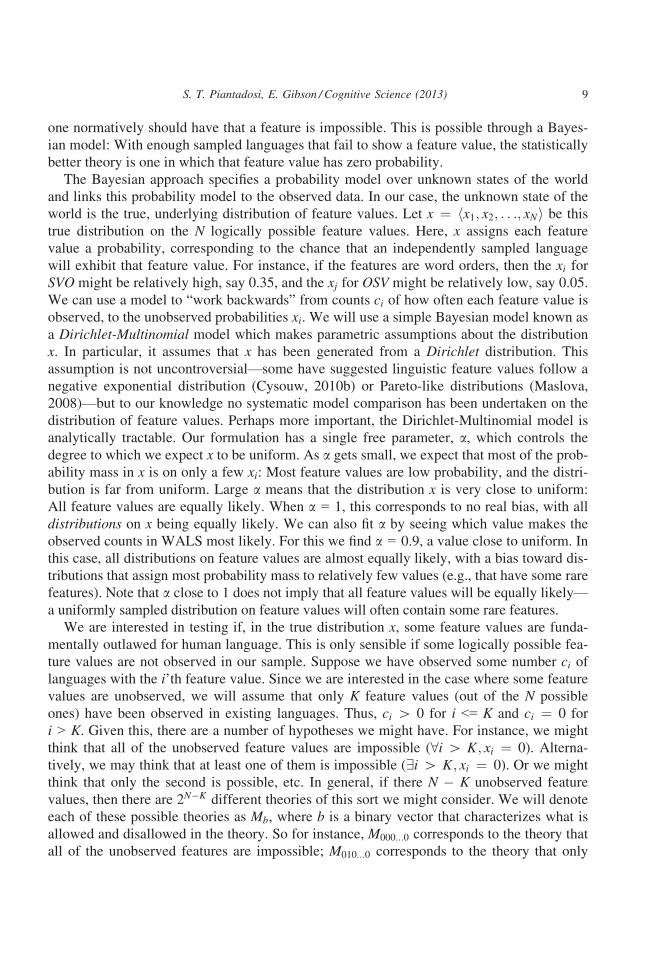
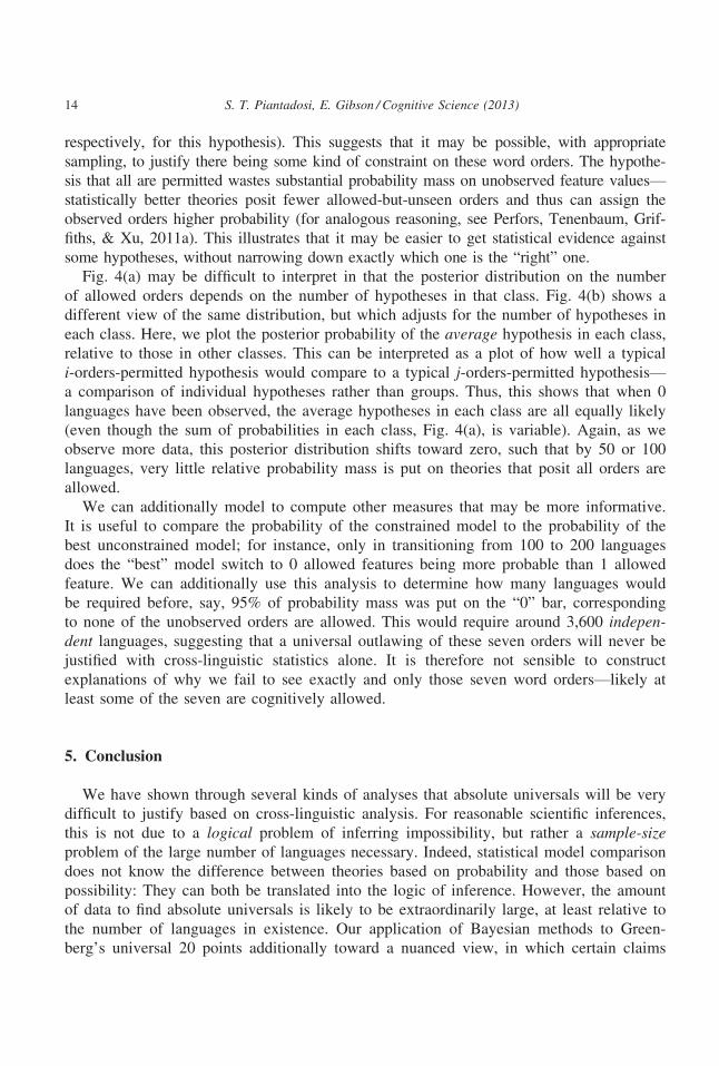
Fig. 1 shows how often one would conclude that each word order is impossible, as the

number of languages sampled, L, varies from 1 to 2,000 languages. In this plot, for

instance, the line for OVS line represents the probability that a scientist who looked at Llanguages would incorrectly conclude that OVS is absolutely and universally outlawed.

We are interested in making the probability of false positives small, below for instance

the dashed 0.05 line or the 0.01 line. This graph illustrates several key points. First—and

unfortunately—this figure shows that for word order, one must have examined a relatively

large number of languages in order to make the false positive probability below 0.05. A

linguist who looked at fewer than around 900 languages would have a false positive rate


of greater than 0.05 of thinking that OSV is an impossible word order. To make the rate

less than 0.01, one would have to look at around 1,400 languages. For our purposes, these

are even slightly conservative6 estimate since we may be interested in the probability of

any feature value rendering a false positive, not just the least frequent one.

Second, this graph illustrates that finding the least frequent feature values is hardest.

This is because they are least likely to be drawn on any individual sample, and so are the

most likely not to occur in a collection of L samples. This should be intuitive, and it

illustrates an often discussed problem for typology: Rare feature values are more difficult

to find, so it is never clear whether a feature value is impossible—or rare and simply not

yet observed (see Cysouw, 2005b, 2010a,b; Wohlgemuth & Cysouw, 2010a, b). In gen-

eral, then, our degree of belief in an absolute universal should depend on how likely the

rarest feature values are.

3. Bootstrapping features from WALS

The analysis in the previous section raises two interesting issues. First, since the false

positive rate depends on how rare the rarest features are, it is not clear that findings based

on the distribution of word orders generalize to other features linguists might care about.

It may be that rare word orders are much rarer than other typical features one would

study, for instance. To address this, we study 138 features from WALS,7 not just word

order. Keeping the false positive rate low across this broader range of features should

provide good guidelines for how to keep the false positive rates low for future linguistic

features which are similar to those already in WALS.

Second, it is not clear that the raw distribution of features in observed languages pro-

vides a good estimate of the true distribution. Many of the languages in WALS are genet-

0 500 1000 1500 2000

0.00

0.05

0.10

0.15

0.20

0.25

Number of languages observed

P(n

ot o

bser

ving

wor

d or

der)

OSVOVSVOSVSOND

SVOSOV

Fig. 1. The probability of thinking that each word order is impossible, as a function of the number of lan-

guages observed.


ically and historically related, meaning that accidents of linguistic history may be driving

the overall distribution of word orders (e.g., Dunn et al., 2011). This means that when we

model sampling from the observed distribution, we are not correctly approximating the

“true” distribution of word orders, and thus not approximating the correct false positive

rate. Here, we consider four methods of approximating the true distribution:

1. Flat sampling—This uses the raw distribution of feature values observed in WALS.

2. Family stratified— Sampling from the true distribution is done by first sampling a

language family uniformly at random, and then sampling a language within that

family uniformly at random.

3. Genus stratified—Sampling from the true distribution is done by first sampling a

language genus uniformly at random, and then sampling a language within that

genus uniformly at random.

4. Independent sample—This method constructs a set of languages which share as

few features as possible, and treats sampling from the true distribution as sampling

from that set of approximately independent languages.

The flat sampling method is the one used in the previous section, using just the raw

feature counts from WALS. The family stratified method attempts to correct for the fact

that imbalances in the number of languages observed in each language family are likely

due to historical accidents (though see Maslova, 2000). We can partially correct for these

historical accidents by increasing the probability with which we sample languages from

language families with fewer languages; we do this by first sampling a family and then

sampling a language in a family. The genus stratified sampling does the same thing, but

at the level of genera rather than families.8 The independent subsample method is meant

to approximate the true distribution by the distribution of features in a sample of

languages whose features are as uncorrelated as possible (see Perkins, 1989; Rijkhof &

Bakker, 1998; Rijkhoff et al., 1993). This also attempts to remove artifacts of history but

does it by finding a sample of languages which is as independent as possible in their

feature values. To do this, we used a simple greedy algorithm to find a diverse subset of

languages.9 We ran this algorithm to produce a set containing 255 and 639 languages,

respectively, 10% and 25% of languages mentioned in WALS.

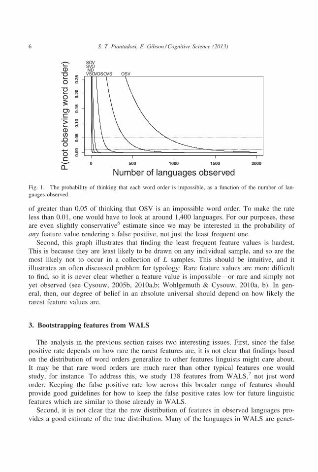
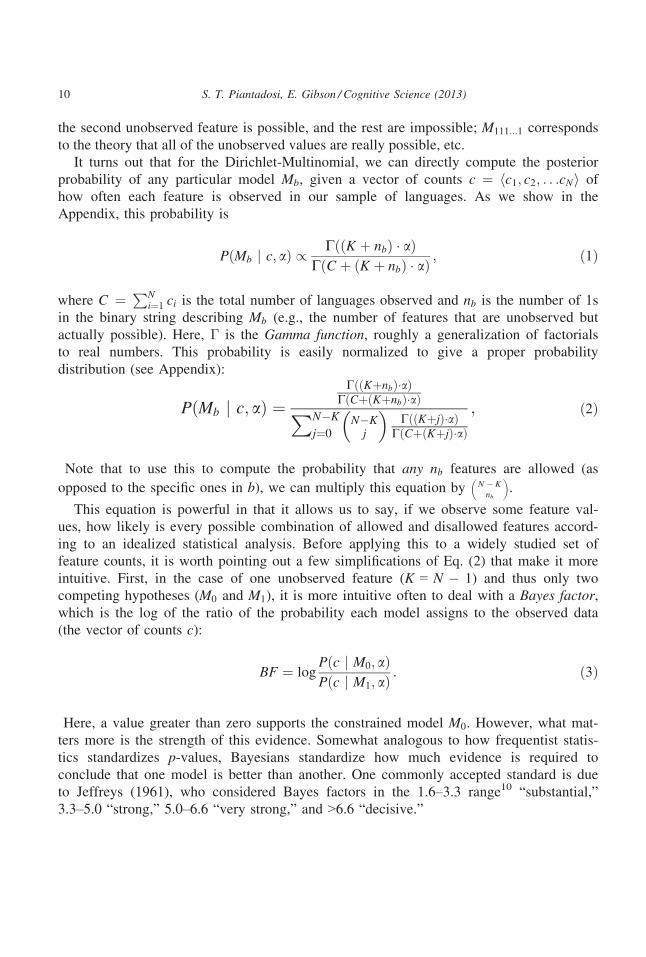
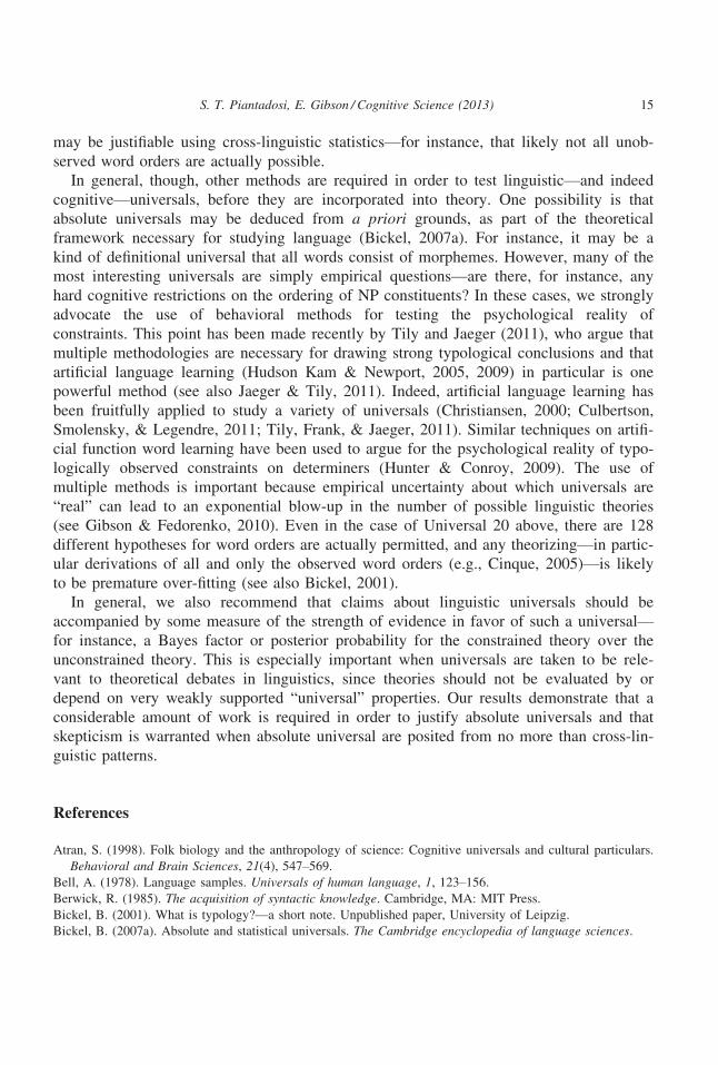
With each of these sampling methods, we used a dynamic programming algorithm to

compute the probability of making a false positive error, averaging across 138 features from

WALS (Fig. 2). Fig. 2 shows the mean false positive rate for various L. The resulting value

can be interpreted as the expected false positive rate for a new feature, given that the new

feature we study is similar to the typical feature already included in WALS (e.g., similar

number and distribution of feature values). This figure demonstrates that the number of lan-

guages necessary to achieve a false positive rate of 0.05 varies from around 250 to nearly

1,500, depending on which sampling method is used to approximate the true distribution.

The most optimistic curve, “Independent sample 10%,” drops below a false positive rate of

0.01 only after 500 languages; some of the others do not make it there even after 2,000 sam-

ples. A rough heuristic one could draw from these plots, then, is that absolute universals are

only likely to truly reflect strong cognitive constraints when they have been examined in at


least 500 independent languages. Note that this provides only a statistical argument of the

impossibility of a feature—a scientist who concluded it was impossible after examining 500

languages would tend to have a reasonably low false positive rate of positing universals.

It is important to emphasize one aspect of this analysis. The sampling procedure we

use assumed independent samples from the true distribution. This means that what is

really required is 500 independent languages, not 500 languages overall. For instance,

Spanish and Italian do not count as two separate languages in this analysis since they are

genetically related. This means that the real number of languages necessary may be much

larger than 500 when sampling uses non-independent languages. Correlated samples will

probably increase the number of samples needed to stay below a given false positive rate.

Note, though, that the languages need not be independent in all respects: They need only

be independent with respect to the relevant feature, which may be possible in some cases.

To the best of our knowledge, it will in general not be possible to find 500 independent

languages. There are, for instance, 212 language families in WALS, yet language families

already are not independent samples. More aggressive independence methods—based on,

for instance, geography (e.g., Dryer, 1989)—will likely arrive at much more independent

samples, but orders of magnitude fewer of them. This means that it is very unlikely that

statistical analysis will provide sufficient evidence to justify absolute universals.

4. A Bayesian approach

In the previous section, we looked at how many samples are necessary to maintain a low

false positive rate using the simulated false positive rates on current data as a proxy for false

positive rates on future data. An alternative approach is to compute the degree of belief that

0 500 1000 1500 2000

0.00

0.10

0.20

Number of languages sampled

Fals

e po

sitiv

e pr

obab

ility

FlatFamilyGenusIndependent sample (10%)Independent sample (25%)

Fig. 2. Bootstrapped false positive rates for 138 features from WALS. This shows the mean false positive

rate across features, taking the average over particular feature values. Thus, this can be interpreted as an esti-

mate of the false positive rate for a newly studied linguistic feature, assuming that its distribution of feature

value is like those observed previously in WALS.


one normatively should have that a feature is impossible. This is possible through a Bayes-

ian model: With enough sampled languages that fail to show a feature value, the statistically

better theory is one in which that feature value has zero probability.

The Bayesian approach specifies a probability model over unknown states of the world

and links this probability model to the observed data. In our case, the unknown state of the

world is the true, underlying distribution of feature values. Let x ¼ hx1; x2; . . .; xNi be this

true distribution on the N logically possible feature values. Here, x assigns each feature

value a probability, corresponding to the chance that an independently sampled language

will exhibit that feature value. For instance, if the features are word orders, then the xi forSVO might be relatively high, say 0.35, and the xj for OSV might be relatively low, say 0.05.

We can use a model to “work backwards” from counts ci of how often each feature value is

observed, to the unobserved probabilities xi. We will use a simple Bayesian model known as

a Dirichlet-Multinomial model which makes parametric assumptions about the distribution

x. In particular, it assumes that x has been generated from a Dirichlet distribution. Thisassumption is not uncontroversial—some have suggested linguistic feature values follow a

negative exponential distribution (Cysouw, 2010b) or Pareto-like distributions (Maslova,

2008)—but to our knowledge no systematic model comparison has been undertaken on the

distribution of feature values. Perhaps more important, the Dirichlet-Multinomial model is

analytically tractable. Our formulation has a single free parameter, a, which controls the

degree to which we expect x to be uniform. As a gets small, we expect that most of the prob-

ability mass in x is on only a few xi: Most feature values are low probability, and the distri-

bution is far from uniform. Large a means that the distribution x is very close to uniform:

All feature values are equally likely. When a = 1, this corresponds to no real bias, with all

distributions on x being equally likely. We can also fit a by seeing which value makes the

observed counts in WALS most likely. For this we find a = 0.9, a value close to uniform. In

this case, all distributions on feature values are almost equally likely, with a bias toward dis-

tributions that assign most probability mass to relatively few values (e.g., that have some rare

features). Note that a close to 1 does not imply that all feature values will be equally likely—a uniformly sampled distribution on feature values will often contain some rare features.

We are interested in testing if, in the true distribution x, some feature values are funda-

mentally outlawed for human language. This is only sensible if some logically possible fea-

ture values are not observed in our sample. Suppose we have observed some number ci oflanguages with the i’th feature value. Since we are interested in the case where some feature

values are unobserved, we will assume that only K feature values (out of the N possible

ones) have been observed in existing languages. Thus, ci [ 0 for i <= K and ci ¼ 0 for

i > K. Given this, there are a number of hypotheses we might have. For instance, we might

think that all of the unobserved feature values are impossible (8i [ K; xi ¼ 0). Alterna-

tively, we may think that at least one of them is impossible (9i [ K; xi ¼ 0). Or we might

think that only the second is possible, etc. In general, if there N � K unobserved feature

values, then there are 2N�K different theories of this sort we might consider. We will denote

each of these possible theories as Mb, where b is a binary vector that characterizes what is

allowed and disallowed in the theory. So for instance, M000...0 corresponds to the theory that

all of the unobserved features are impossible; M010...0 corresponds to the theory that only


the second unobserved feature is possible, and the rest are impossible; M111...1 corresponds

to the theory that all of the unobserved values are really possible, etc.

It turns out that for the Dirichlet-Multinomial, we can directly compute the posterior

probability of any particular model Mb, given a vector of counts c ¼ hc1; c2; . . .cNi of

how often each feature is observed in our sample of languages. As we show in the

Appendix, this probability is

PðMb j c; aÞ / CððK þ nbÞ � aÞCðC þ ðK þ nbÞ � aÞ ; ð1Þ

where C ¼ PNi¼1 ci is the total number of languages observed and nb is the number of 1s

in the binary string describing Mb (e.g., the number of features that are unobserved but

actually possible). Here, Γ is the Gamma function, roughly a generalization of factorials

to real numbers. This probability is easily normalized to give a proper probability

distribution (see Appendix):

PðMb j c; aÞ ¼CððKþnbÞ�aÞ

CðCþðKþnbÞ�aÞPN�K

j¼0N�Kj

� �CððKþjÞ�aÞ

CðCþðKþjÞ�aÞ; ð2Þ

Note that to use this to compute the probability that any nb features are allowed (as

opposed to the specific ones in b), we can multiply this equation by N � Knb

� �.

This equation is powerful in that it allows us to say, if we observe some feature val-

ues, how likely is every possible combination of allowed and disallowed features accord-

ing to an idealized statistical analysis. Before applying this to a widely studied set of

feature counts, it is worth pointing out a few simplifications of Eq. (2) that make it more

intuitive. First, in the case of one unobserved feature (K = N � 1) and thus only two

competing hypotheses (M0 and M1), it is more intuitive often to deal with a Bayes factor,which is the log of the ratio of the probability each model assigns to the observed data

(the vector of counts c):

BF ¼ logPðc j M0; aÞPðc j M1; aÞ : ð3Þ

Here, a value greater than zero supports the constrained model M0. However, what mat-

ters more is the strength of this evidence. Somewhat analogous to how frequentist statis-

tics standardizes p-values, Bayesians standardize how much evidence is required to

conclude that one model is better than another. One commonly accepted standard is due

to Jeffreys (1961), who considered Bayes factors in the 1.6–3.3 range10 “substantial,”

3.3–5.0 “strong,” 5.0–6.6 “very strong,” and >6.6 “decisive.”


The Appendix shows that when a = 1 and K = N � 1, this Bayes factor is simply

BF ¼ logC þ K

K: ð4Þ

For example, to get strong evidence—say, a Bayes factor of 4.0—in favor of a universal

restriction against a single feature value when N = 10 feature values are possible, we

would require a sample of 24 � ð10� 1Þ � 10þ 1 ¼ 135 independently sampled

languages not showing the feature. “Decisive” evidence, a Bayes factor of 6.6, would

require 864 samples. When C ≫ K, the Bayes factor is approximately log (C/K), whichindicates that doubling the number of possible feature values requires roughly doubling

the number of samples, to maintain the same Bayes factor. Note that these results are still

assuming that ci ¼ 0 for i > K; otherwise observing a language with ci [ 0 for some

i > K would falsify model M0. One other important fact about (4) is that as C ? ∞, theBayes factor in favor of M0, with an outlawed feature, will also go to ∞. This means that

as more and more languages are observed, evidence accumulates in favor of a universally

outlawed feature—it is possible to go from frequency counts to statistical inferences of

impossibility. This same fact holds for the more general case of (2): Increased observa-

tions of languages will eventually push the evidence in favor of an absolute restriction,

eventually beyond any fixed standard of evidence.

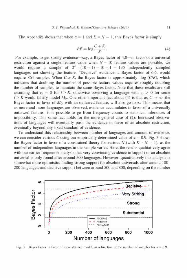
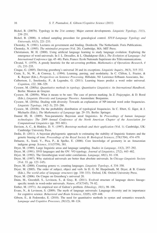
To understand this relationship between number of languages and amount of evidence,

we can consider various C using our empirically determined value of a = 0.9. Fig. 3 shows

the Bayes factor in favor of a constrained theory for various N (with K = N � 1), as the

number of independent languages in the sample varies. Here, the results qualitatively agree

with our earlier frequentist analysis that very convincing evidence in support of an absolute

universal is only found after around 500 languages. However, quantitatively this analysis is

somewhat more optimistic, finding strong support for absolute universals after around 100–200 languages, and decisive support between around 500 and 800, depending on the number

0 200 400 600 800 1000

02

46

8

Number of languages

Bay

es F

acto

r

Substantial

Strong

Very Strong

Decisive

N=3,K=2N=5,K=4N=10,K=9

Fig. 3. Bayes factor in favor of a constrained model, as a function of the number of samples for a = 0.9.


of features examined. Like the above analysis, these languages are required to be indepen-

dent, meaning that even a few hundred languages may be unachievable.

We note, however, that the particulars of this Bayesian analysis are sensitive to a, theparameter expressing how strongly we should expect a uniform distribution of features.

For instance, if a = 0.5, a prior favoring the likelihood of rare features, the most optimis-

tic line only approaches “very strong” evidence after about 800 samples. Conversely, if

a = 2.0, meaning that we expect all feature values are pretty likely, the lines all become

“decisive” before even 200 samples. Unfortunately, this would still be a huge number of

independent languages to find.

One additional advantage of the Dirichlet-Multinomial is that it allows for easy compu-

tation of relevant measures other than the Bayes factor. For instance, we can compute the

expected value that the unconstrained model assigns to one of the N � K unobserved

features. In this case, the probability distribution on feature probabilities given by the

Dirichlet-Multinomial is a Beta distribution xi � Betaða; ðN � 1Þa þ CÞ; in particular,

the unobserved features have an expected probability of a/(Na + C). For instance, in the

unconstrained model, with N = 5, K = 4, a = 0.9, observing one missing feature value

over 100 languages will lead us to believe than an unobserved feature has probability

0.9/(5 � 0.9 + 100) = 0.0086 of being found in a human language. This is a useful

computation for testing typicality universals—we can estimate how infrequent a feature

value is likely to be, given that it has not been observed. Thus, the model can be

used to compute other relevant comparisons and statistics, allowing for more precise

inferences.

4.1. Example computation: Absolute constraints on NP constituent ordering

We next demonstrate how the formal model can be applied to an open area of

research. This example is intended to be illustrative and not conclusive: The right

“answer” will depend on how many effectively independent samples are included in the

world’s extant languages, a difficult problem that is beyond the scope of the current arti-

cle. A considerable amount of work has been done elaborating on Greenberg’s (1963)

Universal 20 (Cinque, 2005; Cysouw, 2010a; Hawkins, 1983; Rijkhoff, 1990, 1998,

2002), which concerns the order of demonstratives, numerals, adjectives, and the head

noun. Only a subset of the possible orderings are observed in human language. The pro-

posals for why some of the noun phrase constituent orderings are unobserved are quite

varied, ranging from explanations internal to Chomsky’s (1995) minimalism (Cinque,

2005), to statistical models based on the properties of the word order (for comparison of

models, see Cysouw, 2010a). This means that the validity of this universal has theoretical

importance.

For this potential universal, we can take Eq. (2) and compute the posterior distribution

for how likely it is that in a sample of languages we should believe any particular con-

straints on allowed features. We use the reported counts from Cysouw (2010a), building

on Dryer (2006), who found that in a sample of 276 languages, 7 of the possible 24


orders (feature values) were unobserved. As above, this means that there are 27 ¼ 128

possible theories for which subset of the unobserved orders is actually cognitively permit-

ted. For simplicity, we will assume a uniform prior on these hypotheses.11 In general,

these 128 hypotheses can be grouped into 7 + 1 = 8 classes for how many of the unob-

served orders really are possible. Note that each class of hypotheses is a different size:

The class where 0 orders are allowed has only one hypothesis (M0000000), the class where

one order is allowed has seven hypotheses (M0000001, M0000010, M0000100, etc.), and in

general the class with i allowed orders has 7

i

� �hypotheses.

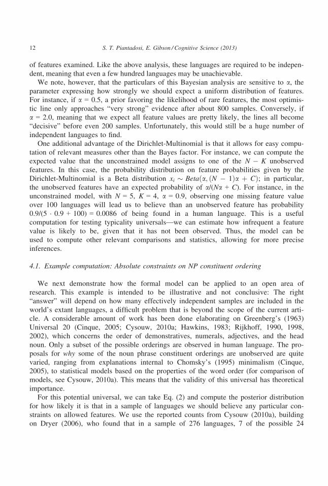
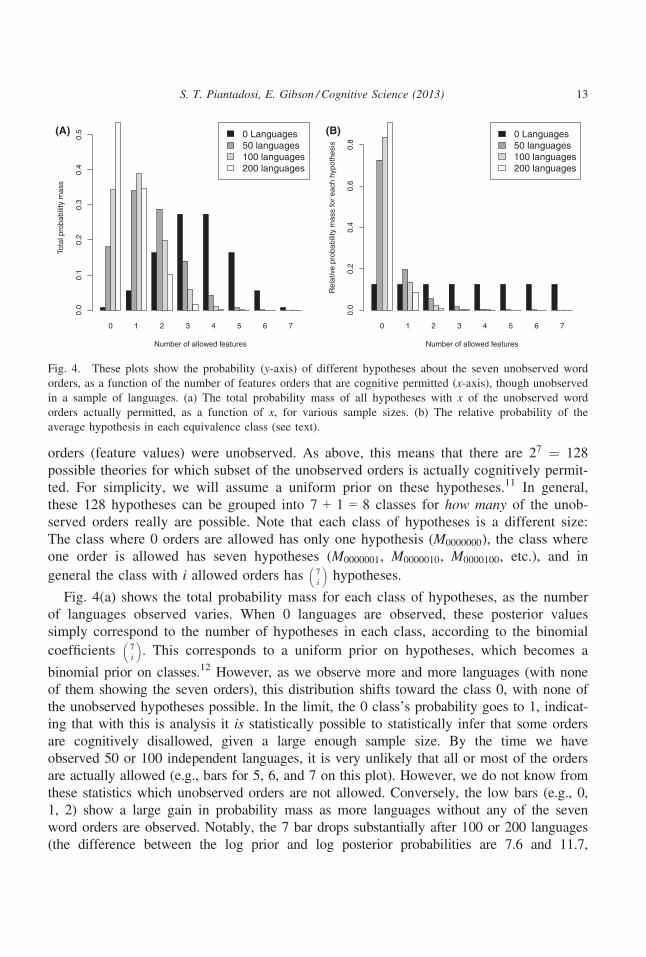
Fig. 4(a) shows the total probability mass for each class of hypotheses, as the number

of languages observed varies. When 0 languages are observed, these posterior values

simply correspond to the number of hypotheses in each class, according to the binomial

coefficients 7

i

� �. This corresponds to a uniform prior on hypotheses, which becomes a

binomial prior on classes.12 However, as we observe more and more languages (with none

of them showing the seven orders), this distribution shifts toward the class 0, with none of

the unobserved hypotheses possible. In the limit, the 0 class’s probability goes to 1, indicat-

ing that with this is analysis it is statistically possible to statistically infer that some orders

are cognitively disallowed, given a large enough sample size. By the time we have

observed 50 or 100 independent languages, it is very unlikely that all or most of the orders

are actually allowed (e.g., bars for 5, 6, and 7 on this plot). However, we do not know from

these statistics which unobserved orders are not allowed. Conversely, the low bars (e.g., 0,

1, 2) show a large gain in probability mass as more languages without any of the seven

word orders are observed. Notably, the 7 bar drops substantially after 100 or 200 languages

(the difference between the log prior and log posterior probabilities are 7.6 and 11.7,

Number of allowed features

Tota

l pro

babi

lity

mas

s

0 Languages50 languages100 languages200 languages

Number of allowed features

Rel

ativ

e pr

obab

ility

mas

s fo

r ea

ch h

ypot

hesi

s7

0.0

0.1

0.2

0.3

0.4

0.5

0 1 2 3 4 5 6 0 1 2 3 4 5 6 7

0.0

0.2

0.4

0.6

0.8

0 Languages50 languages100 languages200 languages

(A) (B)

Fig. 4. These plots show the probability (y-axis) of different hypotheses about the seven unobserved word

orders, as a function of the number of features orders that are cognitive permitted (x-axis), though unobserved

in a sample of languages. (a) The total probability mass of all hypotheses with x of the unobserved word

orders actually permitted, as a function of x, for various sample sizes. (b) The relative probability of the

average hypothesis in each equivalence class (see text).


respectively, for this hypothesis). This suggests that it may be possible, with appropriate

sampling, to justify there being some kind of constraint on these word orders. The hypothe-

sis that all are permitted wastes substantial probability mass on unobserved feature values—statistically better theories posit fewer allowed-but-unseen orders and thus can assign the

observed orders higher probability (for analogous reasoning, see Perfors, Tenenbaum, Grif-

fiths, & Xu, 2011a). This illustrates that it may be easier to get statistical evidence against

some hypotheses, without narrowing down exactly which one is the “right” one.

Fig. 4(a) may be difficult to interpret in that the posterior distribution on the number

of allowed orders depends on the number of hypotheses in that class. Fig. 4(b) shows a

different view of the same distribution, but which adjusts for the number of hypotheses in

each class. Here, we plot the posterior probability of the average hypothesis in each class,

relative to those in other classes. This can be interpreted as a plot of how well a typical

i-orders-permitted hypothesis would compare to a typical j-orders-permitted hypothesis—a comparison of individual hypotheses rather than groups. Thus, this shows that when 0

languages have been observed, the average hypotheses in each class are all equally likely

(even though the sum of probabilities in each class, Fig. 4(a), is variable). Again, as we

observe more data, this posterior distribution shifts toward zero, such that by 50 or 100

languages, very little relative probability mass is put on theories that posit all orders are

allowed.

We can additionally model to compute other measures that may be more informative.

It is useful to compare the probability of the constrained model to the probability of the

best unconstrained model; for instance, only in transitioning from 100 to 200 languages

does the “best” model switch to 0 allowed features being more probable than 1 allowed

feature. We can additionally use this analysis to determine how many languages would

be required before, say, 95% of probability mass was put on the “0” bar, corresponding

to none of the unobserved orders are allowed. This would require around 3,600 indepen-dent languages, suggesting that a universal outlawing of these seven orders will never be

justified with cross-linguistic statistics alone. It is therefore not sensible to construct

explanations of why we fail to see exactly and only those seven word orders—likely at

least some of the seven are cognitively allowed.

5. Conclusion

We have shown through several kinds of analyses that absolute universals will be very

difficult to justify based on cross-linguistic analysis. For reasonable scientific inferences,

this is not due to a logical problem of inferring impossibility, but rather a sample-sizeproblem of the large number of languages necessary. Indeed, statistical model comparison

does not know the difference between theories based on probability and those based on

possibility: They can both be translated into the logic of inference. However, the amount

of data to find absolute universals is likely to be extraordinarily large, at least relative to

the number of languages in existence. Our application of Bayesian methods to Green-

berg’s universal 20 points additionally toward a nuanced view, in which certain claims


may be justifiable using cross-linguistic statistics—for instance, that likely not all unob-

served word orders are actually possible.

In general, though, other methods are required in order to test linguistic—and indeed

cognitive—universals, before they are incorporated into theory. One possibility is that

absolute universals may be deduced from a priori grounds, as part of the theoretical

framework necessary for studying language (Bickel, 2007a). For instance, it may be a

kind of definitional universal that all words consist of morphemes. However, many of the

most interesting universals are simply empirical questions—are there, for instance, any

hard cognitive restrictions on the ordering of NP constituents? In these cases, we strongly

advocate the use of behavioral methods for testing the psychological reality of

constraints. This point has been made recently by Tily and Jaeger (2011), who argue that

multiple methodologies are necessary for drawing strong typological conclusions and that

artificial language learning (Hudson Kam & Newport, 2005, 2009) in particular is one

powerful method (see also Jaeger & Tily, 2011). Indeed, artificial language learning has

been fruitfully applied to study a variety of universals (Christiansen, 2000; Culbertson,

Smolensky, & Legendre, 2011; Tily, Frank, & Jaeger, 2011). Similar techniques on artifi-

cial function word learning have been used to argue for the psychological reality of typo-

logically observed constraints on determiners (Hunter & Conroy, 2009). The use of

multiple methods is important because empirical uncertainty about which universals are

“real” can lead to an exponential blow-up in the number of possible linguistic theories

(see Gibson & Fedorenko, 2010). Even in the case of Universal 20 above, there are 128

different hypotheses for word orders are actually permitted, and any theorizing—in partic-

ular derivations of all and only the observed word orders (e.g., Cinque, 2005)—is likely

to be premature over-fitting (see also Bickel, 2001).

In general, we also recommend that claims about linguistic universals should be

accompanied by some measure of the strength of evidence in favor of such a universal—for instance, a Bayes factor or posterior probability for the constrained theory over the

unconstrained theory. This is especially important when universals are taken to be rele-

vant to theoretical debates in linguistics, since theories should not be evaluated by or

depend on very weakly supported “universal” properties. Our results demonstrate that a

considerable amount of work is required in order to justify absolute universals and that

skepticism is warranted when absolute universal are posited from no more than cross-lin-

guistic patterns.

References

Atran, S. (1998). Folk biology and the anthropology of science: Cognitive universals and cultural particulars.

Behavioral and Brain Sciences, 21(4), 547–569.Bell, A. (1978). Language samples. Universals of human language, 1, 123–156.Berwick, R. (1985). The acquisition of syntactic knowledge. Cambridge, MA: MIT Press.

Bickel, B. (2001). What is typology?—a short note. Unpublished paper, University of Leipzig.

Bickel, B. (2007a). Absolute and statistical universals. The Cambridge encyclopedia of language sciences.


Bickel, B. (2007b). Typology in the 21st century: Major current developments. Linguistic Typology, 11(1),239–251.

Bickel, B. (2008). A refined sampling procedure for genealogical control. STUF-Language Typology andUniversals, 61(3), 221–233.

Chomsky, N. (1981). Lectures on government and binding. Dordrecht, The Netherlands: Foris Publications.

Chomsky, N. (1995). The minimalist program (Vol. 28). Cambridge, MA: MIT Press.

Christiansen, M. H. (2000). Using artificial language learning to study language evolution: Exploring the

emergence of word universals. In J. L. Dessalles, & L. Ghadakpour (Eds.), The Evolution of Language: 3rdInternational Conference (pp. 45–48). Paris, France: Ecole Nationale Sup�erieure des T�el�ecommunications.

Chvatal, V. (1979). A greedy heuristic for the set-covering problem. Mathematics of Operations Research, 4(3), 233–235.

Cinque, G. (2005). Deriving greenberg’s universal 20 and its exceptions. Linguistic Inquiry, 36(3), 315–332.Crain, S., Ni, W., & Conway, L. (1994). Learning, parsing, and modularity. In C. Clifton, L. Frazier, &

K. Rayner (Eds.), Perspectives on Sentence Processing. Hillsdale, NJ: Lawrence Erlbaum Associates, Inc.

Culbertson, J., Smolensky, P., & Legendre, G. (2011). Learning biases predict a word order universal.

Cognition, 122, 306–329.Cysouw, M. (2005a). Quantitative methods in typology. Quantitative Linguistics: An International Handbook.

Berlin: Mouton de Gruyter.

Cysouw, M. (2005b). What it means to be rare: The case of person marking. In Z. Frajzyngier, & D. Rood

(Eds.), Linguistic Diversity and Language Theories. Amsterdam: Benjamins.

Cysouw, M. (2010a). Dealing with diversity: Towards an explanation of NP-internal word order frequencies.

Linguistic Typology, 14(2–3), 253–286.Cysouw, M. (2010b). On the probability distribution of typological frequencies. In C. Ebert, G. J€ager, & J.

Michaelis (Eds.), The Mathematics of Language (pp. 29–35). Berlin: Springer.Daum�e III, H. (2009). Non-parametric Bayesian areal linguistics. In Proceedings of human language

technologies: The 2009 Annual Conference of the North American Chapter of the Association forComputational Linguistics (pp. 593–601).

Davison, A. C., & Hinkley, D. V. (1997). Bootstrap methods and their application (Vol. 1). Cambridge, UK:

Cambridge University Press.

Dediu, D. (2011). A bayesian phylogenetic approach to estimating the stability of linguistic features and the

genetic biasing of tone. Proceedings of the Royal Society B: Biological Sciences, 278(1704), 474–479.Dehaene, S., Izard, V., Pica, P., & Spelke, E. (2006). Core knowledge of geometry in an Amazonian

indigene group. Science, 311(5759), 381.Dryer, M. (1989). Large linguistic areas and language sampling. Studies in Language, 13(2), 257–292.Dryer, M. (1991). SVO languages and the OV: VO typology. Journal of Linguistics, 27(2), 443–482.Dryer, M. (1992). The Greenbergian word order correlations. Language, 68(1), 81–138.Dryer, M. (1997). Why statistical universals are better than absolute universals. In Chicago Linguistic Society

(Vol. 33, pp. 123–145).Dryer, M. (2000). Counting genera vs. counting languages. Linguistic Typology, 4, 334–350.Dryer, M. (2005). The order of subject, object and verb. In D. G. M. Haspelmath, M. Dryer, & B. Comrie

(Eds.), The world atlas of language structures (pp. 330–333). Oxford, UK: Oxford University Press.

Dryer, M. (2006). On Cinque on Greenberg’s universal 20.

Dunn, M., Greenhill, S., Levinson, S., & Gray, R. (2011). Evolved structure of language shows lineage-

specific trends in word-order universals. Nature, 473(7345), 79–82.Ember, M. (1971). An empirical test of Galton’s problem. Ethnology, 10(1), 98–106.Evans, N., & Levinson, S. (2009). The myth of language universals: Language diversity and its importance

for cognitive science. Behavioral and Brain Sciences, 32(05), 429–448.Gibson, E., & Fedorenko, E. (2010). The need for quantitative methods in syntax and semantics research.

Language and Cognitive Processes, 28(1/2), 88–124.


Greenberg, J. (1963). Some universals of grammar with particular reference to the order of meaningful

elements. In Universals of grammar, 73–113. Cambridge, MA: MIT Press.

Hale, M., & Reiss, C. (2003). The subset principle in phonology: Why the tabula can’t be rasa. Journal ofLinguistics, 39(02), 219–244.

Haspelmath, M. (2004). Does linguistic explanation presuppose linguistic description? Studies in Language,28(3), 554–579.

Haspelmath, M., & Siegmund, S. (2006). Simulating the replication of some of Greenberg’s word order

generalizations. Linguistic Typology, 10, 74–82.Haspelmath, M., Dryer, M., Gil, D., & Comrie, B. (2005). The World Atlas of Language Structures Online.

Hauser, M., Chomsky, N., & Fitch, W. (2002). The faculty of language: What is it, who has it, and how did

it evolve? Science, 298(5598), 1569.Hawkins, J. (1983). Word order universals: Quantitative analyses of linguistic structure. New York:

Academic Press.

Hudson Kam, C., & Newport, E. (2005). Regularizing unpredictable variation: The roles of adult and child

learners in language formation and change. Language Learning and Development, 1(2), 151–195.Hudson Kam, C., & Newport, E. (2009). Getting it right by getting it wrong: When learners change

languages. Cognitive Psychology, 59(1), 30–66.Hunter, T., & Conroy, A. (2009). Children’s restrictions on the meanings of novel determiners: An

investigation of conservativity. In J. Chandlee, M. Franchini, S. Lord, & G.-M. Rheiner (Eds.), BUCLD33 proceedings (pp. 245–255). Somerville, MA: Cascadilla Press.

Jaeger, T., & Tily, H. (2011). On language ‘utility’: Processing complexity and communicative efficiency.

Wiley Interdisciplinary Reviews: Cognitive Science, 2(3), 323–335.Janssen, D., Bickel, B., & Z�u~niga, F. (2006). Randomization tests in language typology. Linguistic Typology,

10(3), 419–440.Jeffreys, S. (1961). Theory of probability. Oxford, UK: Oxford University Press.

Kay, P., & Regier, T. (2003). Resolving the question of color naming universals. Proceedings of the NationalAcademy of Sciences, 100(15), 9085.

Maslova, E. (2000). A dynamic approach to the verification of distributional universals. Linguistic Typology,4(3), 307–333.

Maslova, E. (2008). Meta-typological distributions. Language Typology and Universals, 61(3), 199–207.Mikhail, J. (2007). Universal moral grammar: Theory, evidence and the future. Trends in Cognitive Sciences,

11(4), 143–152.Naroll, R. (1973). Galton’s problem. In A handbook of methods in cultural anthropology, (pp. 974–989).

Walnut Creek, CA: Altamira Press.

Newmeyer, F. (1998). The irrelevance of typology for grammatical theory. Syntaxis, 1, 161–197.Newmeyer, F. (2004). Typological evidence and universal grammar. Studies in Language, 28(3), 527–548.Nichols, J. (1992). Linguistic diversity in space and time. University of Chicago Press.

Perfors, A., Tenenbaum, J., & Regier, T. (2011). The learnability of abstract syntactic principles. Cognition,118, 306–338.

Perfors, A., Tenenbaum, J., Griffiths, T., & Xu, F. (2011a). A tutorial introduction to Bayesian models of

cognitive development. Cognition, 120(3), 302–321.Perkins, R. (1989). Statistical techniques for determining language sample size. Studies in Language, 13(2),

293–315.Piantadosi, S., Goodman, N., & Tenenbaum, J. (2013). Modeling the acquisition of quantifier semantics: A

case study in function word learnability. Under review.

Pica, P., Lemer, C., Izard, V., & Dehaene, S. (2004). Exact and approximate arithmetic in an Amazonian

indigene group. Science, 306(5695), 499.Pinker, S., & Bloom, P. (1990). Natural language and natural selection. Behavioral Brain Sciences, 12, 707–784.Rijkhof, J., & Bakker, D. (1998). Language sampling. Linguistic Typologie, 2(2–3), 263–314.Rijkhoff, J. (1990). Explaining word order in the noun phrase. Linguistics, 28(1), 5–42.


Rijkhoff, J. (1998). Order in the noun phrase of the languages of Europe. Empirical Approaches to LanguageTypology, 20, 321–382.

Rijkhoff, J. (2002). The noun phrase. Oxford, UK: Oxford University Press.

Rijkhoff, J., Bakker, D., Hengeveld, K., & Kahrel, P. (1993). A method of language sampling. Studies inLanguage, 17(1), 169–203.

Smolensky, P. (1996). The initial state and ‘richness of the base’ in Optimality Theory (Technical Report).Johns Hopkins University, Department of Cognitive Science. Baltimore, MD

Tily, H., & Jaeger, T. (2011). Complementing quantitative typology with behavioral approaches: Evidence

for typological universals. Linguistic Typology, 15(2), 497–508.Tily, H., Frank, M., & Jaeger, T. (2011). The learnability of constructed languages reflects typological

patterns. In Proceedings of Cognitive Science Society, 33, 1364–1369.Tomlin, R. (1986). Basic word order: Functional principles. Kent, UK: Routledge Kegan & Paul.

Wexler, K., & Culicover, P. (1983). Formal principles of language acquisition. Kent, UK: Cambridge, MA:

MIT Press.

Wexler, K., & Manzini, R. (1984). Parameters and learnability in binding theory. In T. Roeper, & E.

Williams (Eds.), Parameter Setting. Reidel.Wohlgemuth, J., & Cysouw, M. (2010a). Rara & Rarissima: Documenting the fringes of linguistic diversity

(Vol. 46). The Hague: De Gruyter Mouton.

Wohlgemuth, J., & Cysouw, M. (2010b). Rethinking universals: How rarities affect linguistic theory (Vol.

45). The Hague: De Gruyter Mouton.

Xu, F., & Tenenbaum, J. (2007). Sensitivity to sampling in Bayesian word learning. Developmental Science,10(3), 288–297.

Appendix:Derivation of Bayes factor

We apply a simple Bayesian model known as a Dirichlet-Multinomial model which

has been used extensively in machine learning and statistics. We present a derivation for

a model Mb, where b is, as above, a binary string describing which of the unobserved

feature values are in reality impossible. Thus, for instance, M11...1 corresponds to the the-

ory that all unobserved features are possible, and M00...0 corresponds to the theory under

which none are possible. We assume a Dirichlet prior on x, the true distribution of fea-

tures. The Dirichlet prior is given in the following:

Pðx j a;MbÞ ¼ CððK þ nbÞ � aÞCðaÞKþnb

YKþnb

i¼1

xa�1i ; ð5Þ

where nb is, as above, the number of 1s in b. For notational simplicity, our equations will

all assume that the nb ones in b occur in the first nb digits of b: thus, we might have

b = 1100 or b = 1000, but not b = 0100. This assumption simplifies the notation greatly

but does not affect the math—the same derivations can be made by appropriately

shuffling the indices of xi based on which features are allowed via b. This simplification

is why the sum can run to K þ nb, as opposed K, and then some subset of later indices.

This prior has two parts. The fraction out front term is simply a normalizing constant,

written in terms of the Γ-function. The product over xa�1i formalizes the key part of the prior


and is parameterized by the single variable a. As a gets large, this prior favors a uniform dis-

tribution, xi ¼ 1=ðK þ nbÞ for all i. As a gets small, this prior favors distributions that

place probability mass on only a few xi. Crucially, however, this prior treats all xi the same,

meaning that a priori we do not expect some feature values to be more likely than others a

priori.13

The second part of the model is the likelihood, which formalizes how likely the

observed data are for any assumed distribution x. The likelihood takes a simple form as

well. Suppose that the ith logically possible feature value occurs ci times in the observed

data. This happens with probability xcii since each instance occurs with probability xi, andthere are ci of them. Taking into account the fact that the data points can occur in any

order, this means that Pðc j x;MbÞ is then

Pðc j x;MbÞ ¼ CðCÞQKi¼1 CðciÞ

YKþnb

i¼1

xcii ; ð6Þ

with C ¼ PNi¼1 ci. With this likelihood, distributions that closely predict the empirically

observed distribution ci are more likely than those which predict distributions far from

the observed ones.

We are interested in how well Mb can predict the observed counts. Formally, we want

a model such PðMb j c; aÞ is high—the probability of the model given the counts is large.

By Bayes rule, and the independence of Mb and a, we have that

PðMb j c; aÞ / PðMbÞPðc j Mb; aÞ¼ PðMbÞ

ZPðc j x;MbÞPðx j Mb; aÞdx:

ð7Þ

Here, we will consider the priors PðMbÞ / 1, meaning that we are equally likely to

think that each Mb is true a priori; this assumption can be altered if one is willing to keep

track of the PðMbÞ below. Using this, (5) and (6) above, this gives that

PðMb j c; aÞ / CðCÞQKi¼1 CðciÞ

� CððK þ nbÞ � aÞCðaÞKþnb

�Z YKþnb

i¼1

xciþa�1i dx: ð8Þ

Here, the integral is a special form, a type-1 Dirichlet integral, and can be evaluated

analytically to yield,

PðMb j c; aÞ / CðCÞQKi¼1 CðciÞ

� CððK þ nbÞ � aÞCðaÞKþnb

� CðaÞnbQK

i¼1 Cðci þ aÞCðC þ ðK þ nbÞ � aÞ

¼ CðCÞCðaÞK � CððK þ nbÞ � aÞ

CðC þ ðK þ nbÞ � aÞ �YKi¼1

Cðci þ aÞCðciÞ :

ð9Þ

Since this equation is only proportional to the posterior probability PðMb j c; aÞ, we must

normalize it to get actual posterior probabilities. In this step, the first and last terms,


which do not depend on nb (the model) will cancel, giving


CðCþðKþnbÞ�aÞPb0

CððKþnb0 Þ�aÞCðCþðKþnb0 Þ�aÞ

ð10Þ

Notice that the denominator sum runs over all b0, but the term depends only on the

number of 1s in b0, nb0 . This means that we can group together similar elements in the

denominator and rather than have an exponential sum over all binary strings of length

N � K, we can have a smaller (and more numerically stable) sum:


CðCþðKþnbÞ�aÞPN�K

j¼0N�Kj

� �CððKþjÞ�aÞ

CðCþðKþjÞ�aÞ: ð11Þ

This equation, though not mathematically trivial, can easily be computed for any reason-

able number of features.

Note that when a = 1 and K = N � 1, Eq. (11) can be simplified significantly. In this

case of two hypotheses, it is easier to work with the log posterior odds, or the Bayes fac-

tor (Jeffreys, 1961),

logPðc j M0; a ¼ 1ÞPðc j M1; a ¼ 1Þ ¼ log

CðKÞCðCþKÞCðKþ1Þ

CðCþKþ1Þ¼ log

C þ K

K: ð12Þ

Notes

1. We differ from previous literature and Greenberg, which refer to these as statisticaluniversals.

2. This problem known as Galton’s problem, after Sir Francis Galton, who first

pointed out the issues it causes for comparative anthropological work (c.f. Ember,

1971). Some anthropologists have even argued that the problem is so severe, there

exist only 50–75 cultures that can be examined in the whole world and treated

independently (Naroll, 1973); Perkins (1989) argues similarly for linguistic typol-

ogy.

3. Dryer uses “testable” as a technical term, meaning that there exists possible evi-

dence to falsify the theory, and possible evidence to confirm it.

4. This setup is similar in spirit to the principles and parameters approach to lan-

guage acquisition (e.g., Chomsky, 1981; Wexler & Culicover, 1983), but it is

meant to be theory-neutral. The features we describe may be entirely descriptive—there is no assumption that the space of these parameters is, for instance, innate.


5. For simplicity, here we assume that the languages sampled are drawn indepen-

dently, but the topic of independence will be addressed more in the next section.

6. In this article, conservative means we underestimate the number of languages

required. This is conservative with respect to the number required, not with respect

to the estimated false positive rate for any sample size.

7. For simplicity, we take the particular WALS feature values at face value and

assume that they are a reasonable characterization of typical features linguistics

would characterize.

8. We note that both family- and genus-level sampling has been criticized methodo-

logically (e.g., Bickel, 2008; Janssen, Bickel, & Z�u~niga, 2006); in general, our

basic bootstrapping approach supports is amenable to even more sophisticated

means of generating independent subsets of languages, such as areal stratification

(Dryer, 1989, 1991, 1992) or Bayesian phylogenetic methods (Daum�e III, 2009;

Dediu, 2011).

9. Finding the most diverse subset of languages would require searching over the expo-

nentially many subsets of existing languages, creating an instance of the NP-complete

problem SET-COVER. Our algorithm is similar to the best polynomial time

approximation to SET-COVER (Chvatal, 1979). The algorithm starts with an

empty set of languages and considers adding each possible language in WALS. It first

adds languages that decrease the number of unobserved feature values. This ensures

that, with enough languages, all feature values are represented. To break ties, it adds

languages that share the smallest proportion of their defined features with languages

already in the set. Further ties are broken by picking languages that have the largest

number of defined features. Note that after enough languages have been added so that

all feature values are observed, additional languages never decrease the number of

unobserved feature values, meaning that the decision about which language to add is

based first on the proportion of features it shares with languages already in the set.

This creates a set of languages with diverse feature values.

10. Log base 2.

11. An important caveat is that we might actually assign higher prior to M1111111 since

it is in some sense cognitively simpler: It posits no constraints on word order. An

analogous analysis could be applied in this case.

12. Another modeling approach would have been to put a uniform prior on the num-ber of orders which are allowed, instead of the specific set of orders. Doing so

would require almost exactly the same derivations presented in the Appendix and

would have yielded a posterior distribution over the number of disallowed orders

identical to Fig. 4(b).

13. This is a simplification for our purposes, but this same class of model will work

with different prior expectations for each xi.


Quantitative Standards for Absolute Linguistic...

Documents

Transcript of Quantitative Standards for Absolute Linguistic...