Quantitative models for supply chain risk analysis from a ...Quantitative models for supply chain...

Quantitative models for supply chain risk analysis from a firm’s perspective

by

Arun Vinayak

A thesis submitted to the graduate faculty

in partial fulfillment of the requirements for the degree of

MASTER OF SCIENCE

Major: Industrial Engineering

Program of Study Committee:

Cameron A. MacKenzie, Major Professor

Caroline C. Krejci

Scott J Grawe

The student author and the program of study committee are solely responsible for the

content of this dissertation. The Graduate College will ensure this dissertation is globally

accessible and will not permit alterations after a degree is conferred.

Iowa State University

Ames, Iowa

2017

Copyright © Arun Vinayak, 2017. All rights reserved.

ii

DEDICATION

I dedicate this thesis to my mother and my father for their patience and support while I

was away from them to complete my studies. I also dedicate this thesis to my sister for

encouraging me to succeed since we were kids.

iii

TABLE OF CONTENTS

Page

ACKNOWLEDGMENTS ......................................................................................... iv

ABSTRACT………………………………. .............................................................. v

CHAPTER 1 GENERAL INTRODUCTION AND REVIEW OF LITERATURE 1

Research Motivation ............................................................................................ 3

Thesis Organization ............................................................................................. 3

References ......................................................................................................... 4

CHAPTER 2 A QUANTITATIVE MODEL FOR ANALYZING MARKET

RESPONSE DURING SUPPLY CHAIN DISRUPTIONS ...................................... 6

Abstract………………………………. ............................................................... 6

Introduction ......................................................................................................... 7

Literature Review................................................................................................. 9

Model………………………………. .................................................................. 11

Illustrative Example ............................................................................................. 17

Conclusions ......................................................................................................... 24

References ......................................................................................................... 25

CHAPTER 3 COST EFFECTIVENESS ANALYSIS OF SUPPLIER

EFFECTIVENESS BASED ON SCOR METRICS .................................................. 29

Abstract………………………………. ............................................................... 29

Introduction ......................................................................................................... 30

Literature Review................................................................................................. 32

Methodology ........................................................................................................ 35

Illustrative Example ............................................................................................. 53

Conclusions ......................................................................................................... 59

References ......................................................................................................... 61

CHAPTER 5 GENERAL CONCLUSIONS ......................................................... 64

General Discussion .............................................................................................. 64

Recommendations for Future Research ............................................................... 65

APPENDIX A APPROXIMATING VALUE FUNCTIONS IN EXCEL .............. 67

iv

ACKNOWLEDGMENTS

Firstly, I would like to thank my advisor Dr. Cameron MacKenzie for introducing me

to the fascinating world of engineering risk analysis and encouraging me to do research right

from my first semester. I want to express my gratitude for his continuous support, patience,

motivation, and immense knowledge throughout my graduate study and research.

I would like to thank my committee members, Dr. Caroline Krejci and Dr. Scott Grawe

for the guidance and support that they provided to achieve my academic goals. I would also

like to express my gratitude for all my colleagues, mentors, and mangers at Tesla during my

seven-month internship at the Tesla factory in Fremont, CA.

In addition, I want to offer my appreciation to my friends, colleagues, the department

faculty and staff for making my time at Iowa State University a wonderful experience, without

whom, this thesis would not have been possible.

v

ABSTRACT

Supply chain risk analysis garnered increased attention, both in academia and in

practice, since the early 2000s. Modern production methodologies such as just-in-time and lean

manufacturing, globalized supply chains, shorter product life cycle, and the emphasis on

efficiency have increased the risk faced by many supply chains. Managing such risks that is

faced by a supply chain is vital to the success of any company. Currently employed methods

lack consideration of market reaction and incorporation of decision maker preferences in

managing supply chain risk. In this thesis, these two factors are taken into consideration to

develop quantitative methods to analyze supply chain risk.

The first study is focused on supply chain risk from the market side in case of a major

disruption. A probabilistic model based on different types of customer behaviors is developed

to identify the impact on the firm’s revenue by forecasting the lost revenue in case of a

production shut down from a disruption event. Results from a simulation of the developed

model is analyzed to draw useful insights to manage the risk of such an event.

The second study is centered on supplier selection. It presents a 5-step framework based

on KPIs derived from the performance metrics of the SCOR (Supply Chain Operations

Reference) model. The framework can be used for supplier selection as well as for supplier

performance monitoring as the firm continues to work with the selected supplier. Decision

makers from a firm can incorporate their own preference within the presented framework to

determine the most preferred supplier and assess the cost effectiveness to select a supplier in

different scenarios to minimize supply side risk.

1

CHAPTER 1. GENERAL INTRODUCTION AND REVIEW OF

LITERATURE

Risk analysis is a critical process and is widely adopted in many sectors ranging from

manufacturing and retail to logistics and military (Bedford and Cooke, 2001). According to

Kaplan and Garrick (1981), risk is associated with both uncertainty and damage and analyzing

risk consists of answering three questions: 1) What can go wrong? 2) How likely is it that will

happen? and 3) If it does happen, what are the consequences? Getting answers to these

questions by identifying risk factors, their chances of occurrence, and their consequences,

enables a decision maker to devise a plan to manage the risk (Chavas, 2004).

Risk analysis can be conducted through both qualitative and quantitative techniques

and a mix of two, ranging from simple brainstorming to more technical computer stimulation

(Modarres, 2006). The quantitative techniques for risk analysis use estimation method to find

the probability of loss caused by a certain event and the magnitude of the loss (Modarres,

2006). In comparison, qualitative techniques are more flexible and instead of using probability,

they usually use more diverse methods to decide the likelihood and impact of risks. The

qualitative techniques are useful in the prioritization of the risk in accordance with their

likelihood and magnitude of impact (Burtonshaw-Gunn, 2009). The mix of qualitative and

quantitative technique use one of the techniques for measuring chances of loss and another one

for amount of loss (Modarres, 2006).

Among different quantitative techniques for risk analysis, probabilistic method is most

commonly used for studying complex technical systems (Käki, Salo & Talluri, 2013). The

basic technique according to Käki et al. (2013) is to develop a structural model of the system

2

under study, identify the key risk factors and measure their probability of occurrence, and

finally conduct a probabilistic analysis to identify the most-risky segments of systems.

With the onset of global supply chains and outsourcing of suppliers, supply chains have

become more complex in the 21st century. Although the cost can be reduced through

outsourcing suppliers from different parts of the world, it increases the probability of risk as

well as magnitude of loss (Choi and Krause 2006). In addition, the regulations have become

diversified and more complex for a manufacturer to handle without conducting a proper risk

analysis (Sadgrove, 1996). There is also shift in the attitude of clients who have become more

demanding and critical (Sadgrove, 1996). As a result, companies have become more concerned

about risk management than cost management when it comes to supply chain (Simchi-Levi

2010).

According to Waters (2011), each member of the supply chain is subject to some

specified risks from his own activities, from activities of other members of supply chain and

from the factors external to the supply chain. From a manufacturer or firm’s perspective, the

losses can range from delay in supplying finished good to market to their total inability to

continue business. Firms face multiple decision problems where more than one factor

influences the decision maker’s preferences over the best possible outcome. When faced with

such complex problems, decision makers often use simplified mental strategies, or heuristics

due to limited information-processing capacity (Paul & George, 2004). Jüttner (2005) found

that while there is growing awareness among manufacturers on the growing risk associated

with supply chain, they still lack proper understanding of what entailed supply chain risk

management. Improvement of this understanding and introduction of proper supply risk

analysis practices in manufacturing firm is a critical need of the day.

3

Research Motivation

The motivation of this research derives from the need for clear and quantitative

methods to express supply chain risk from the perspective of a firm or a manufacturer so that

in a decision-making process, the firm can weigh risks along with all other costs and benefits.

The objectives of this research are as follows:

1. To develop a method to quantify the risk faced by a firm or a manufacturer from a

severe supply chain disruption with an explicit focus on customer demand.

2. To evaluate the extent to which a firm can be penalized from a supplier default leading

to a temporary production shut-down.

3. To develop an effective framework for supplier selection and evaluation.

4. To derive risk management insights using the developed method and framework.

Thesis Organization

This thesis contains two research papers that constitutes chapters 2-3. The first paper

in chapter 2 attempts to model downstream risk in a supply chain from a firm’s perspective

while the second paper in chapter 3 considers the upstream supply chain and presents a

framework for supplier selection and evaluation. Both the chapters consist of an abstract,

introduction, literature review, methodology, illustrative example, and conclusions.

References that correspond to the in-chapter citations are provided at the end of each chapter.

All the images and tables are first labeled with the chapter they reside followed by the number

of the graphic within the chapter for clarity. The final chapter consist of general conclusions

and future work.

4

References

Bedford, T., & Cooke, R. Probabilistic risk analysis: foundations and methods. 2001.

Cambridge. Univ. Press, UK.Sheffi, Y., & Rice Jr, J. B. (2005). A supply chain view of

the resilient enterprise. MIT Sloan Management Review, 47(1), 41.

BurtonShAw-Gunn, S. A. (2009). Risk and Financial Management in Construction.

Burlington, VT: Ashgate Publishing Company.

Chavas, J. P. (2004). Risk Analysis in Theory and Practice. London, UK: Elsevier Academic

Press.

Choi, T. Y., & Krause, D. R. (2006). The supply base and its complexity: Implications for

transaction costs, risks, responsiveness, and innovation. Journal of Operations

Management, 24(5), 637-652.

Jüttner, U. (2005). Supply chain risk management: Understanding the business requirements

from a practitioner perspective. The International Journal of Logistics Management,

16(1), 120-141.

Käki, A., Salo, A., & Talluri, S. (2015). Disruptions in supply networks: A probabilistic risk

assessment approach. Journal of Business Logistics, 36(3), 273-287.

Kaplan, S., & Garrick, B. J. (1981). On the quantitative definition of risk. Risk analysis, 1(1),

11-27.

Modarres, M. (2006). Risk Analysis in Engineering: techniques, tools, and trends. Boca

Raton, FL: CRC press.

Paul, G., & George, W. (2004). Decision Analysis for Management Judgment.

Simchi-Levi, D. (2010). Operations rules: delivering customer value through flexible

operations. Cambridge, MA: MIT Press.

5

Waters, D. (2011). Supply chain risk management: vulnerability and resilience in logistics

(2nd ed.). Philadelphia, PA: Kogan Page Publishers.

6

CHAPTER 2. A QUANTITATIVE MODEL FOR ANALYZING

MARKET RESPONSE DURING SUPPLY CHAIN DISRUPTIONS

A book chapter accepted for publication in the Springer book Supply Chain Risk

Management: Advanced Tools, Models, and Developments

Arun Vinayak, Cameron A. MacKenzie

Abstract

Supply chain disruptions can lead to firms losing customers and consequently losing profit.

We consider a firm facing a supply chain disruption due to which it is unable to deliver

products for a certain period of time. When the firm is restored, each customer may choose to

return to the firm immediately, with or without backorders, or may purchase from other firms.

This chapter develops a quantitative model of the different customer behaviors in such a

scenario and analytically interprets the impact of these behaviors on the firm’s post-disruption

performance. The model is applied to an illustrative example.

Keywords - Supply Chain Risk Management; Supply Chain Disruption; Preparedness;

Response; Customer Demand

7

1. Introduction

Supply chain disruptions have garnered increased attention, both in academia and in

practice, since the early 2000s. Modern production methodologies, globalized supply chains,

shorter product life cycle, and the emphasis on efficiency have increased the risk faced by

many supply chains. Managing the risk facing a supply chain is vital to the success of any

company.

Fig. 2.1. A simple supply chain model

A supply chain is an integrated system of companies involved in the upstream and

downstream flows of products, services, finances, and/or information from a source to a

customer (Mentzer et al. 2001). Fig. 2.1 presents a basic supply chain model from the firm’s

perspective. A supply chain is characterized by the flow of resources—typically material,

information, and money—with the primary purpose of satisfying the needs of a customer, who

are the source of revenue for a firm. A supply chain will ideally maximize the total value

generated from customers and minimize the cost of meeting consumer demand.

Major disruptions, such as those that occur from natural disasters, terrorist acts, and

labor strikes, can interrupt the flow of materials for several firms. Sodhi and Tang (2012)

categorized supply chain risk into supply risks, process risks, demand risks, and corporate-

level risks. These risks often materialize all together during a major supply chain disruption,

and decision makers need to consider all of these risks. Kilubi and Haasis (2015) conducted a

8

systematic literature review on supply chain risk management (SCRM) and identified ten

different definitions of SCRM. Lavastre et al. (p. 839, 2012) defined SCRM as “the

management of risk that implies both strategic and operational horizons for long-term and

short-term assessment.” As implied by this definition, decision makers need to consider both

the long-term and short-term impacts from a supply chain disruption.

The marketplace or customers can play a significant role in the long-term impacts as

their needs, values, and opinions will affect the firm’s decisions during the disruption. The

volatility of consumer demand is a major form of risk (Jüttner et al. 2003). Firms face a risk of

being penalized by their customers if their suppliers default and firms are unable to deliver on

their obligations. Assessing how consumers react to such disruptions helps to forecast the long-

term profits for the firm and can help it make sound risk management decisions. Modeling

consumer behavior is useful not only when a disaster occurs but also to build flexibility within

the supply chain as a proactive measure to anticipate such threats and quickly respond.

This chapter presents a probabilistic model to quantify the risk from a severe supply

chain disruption with an explicit focus on how consumers or the marketplace’s demand for a

product should influence a firm’s risk management strategies. Many supply chain disruption

models assume some type of demand function, which may be constant or random. However,

that demand function does not usually change when the disruption occurs, or simple

assumptions are made about whether or not customers are willing to wait for a final product.

Less research has focused on how the final customers should influence how a firm determines

what risk management strategies are appropriate. This chapter models the demand function

using a probabilistic approach to customer behavior in a post-disruption scenario. The model

assumes that a disruption causes a supplier to default, and a firm is unable to deliver its product

9

to consumers. The market responds with defined probabilities and time delays. The model

attempts to measure the extent to which a firm can be penalized due to a default from its

supplier and recommends strategies or practices to build resilience to such disruptions.

This chapter is organized as follows: a literature review is given in Section 2. Section

3 presents the mathematical model framework, and Section 4 describes an illustrative example

and performs sensitivity analysis. Section 5 concludes the chapter with recommendations,

insights, and conclusions drawn from the study.

2. Literature Review

Supply chain management has seen a variety of trends, including Just-in-Time, global

sourcing, and outsourcing. These methods are aimed at cutting costs in a firm’s supply chain

and enabling the firm to compete more effectively. Increasing supply chain efficiency can also

make supply chains more vulnerable to disruptions (Christopher 2005). In the race to increase

their market share, firms may ignore that their supply chains are susceptible to disruptions.

A wide variety of events can disrupt a supply chain, including supply-side difficulties,

demand-side variability, operational problems, and large-scale disruptions such as natural

disasters (Manuj et al. 2007). Qualitative studies to manage these disruptions recommend

excess inventory, additional capacity, redundant suppliers, flexible production and

transportation, and dynamic pricing (Sheffi and Rice 2005; Stecke and Kumar 2009).

Managing one type of risk may exacerbate another risk, and identifying the best strategy relies

on the manager’s ability to identify the most crucial risk and understand the trade-offs in

SCRM (Chopra and Sodhi 2004). Quantitative studies in SCRM generally model the trade-off

between purchasing from alternate suppliers and holding inventory (Tomlin and Wang 2005),

10

or they model the interaction between suppliers and customers (Babich et al. 2007; Xia et al.

2011). MacKenzie et al. (2014) used simulation to model the interactions among supply chain

entities where each entity can take different actions such as holding inventory or purchasing

from alternate suppliers. Interested readers should refer to Snyder et al. (2016) for an in-depth

review of the recent models of supply chain disruptions and disruption management strategies.

Although research has focused on the impacts of supply chain disruptions based on

stock returns (Hendricks and Singhal 2005) or based on the economic linkages (MacKenzie et

al. 2012), less research has focused on how customers behave during and after a supply chain

disruption. Nagurney et al. (2005) examined the impact of unforeseen customer demands on

the supply chain, but this research assumes the customer behavior causes the disruption. Ellis

et al. (2010) surveyed managers and buyers of materials to study how customers may perceive

supply chain risk. Modern supply chain management is very sensitive to customer demand

(Nishat Faisal et al. 2006), but examining the relationship between customer demand

sensitivity and a manufacturer or retailer during a disruption has not been fully explored. An

important exception to this lack of research is the modeling and analysis of consumer behavior

following a food contamination (Beach et al. 2008; Arnade et al. 2009).

This chapter seeks to fill the gap in the existing literature by probabilistically modeling

customer behavior following a supply chain disruption. Whereas much of the current literature

focuses on the interaction between the supplier and the firm, the focus of this chapter is the

market response to the disruption and its impact on the firm. The model examines the decisions

customers make after the interruption of a firm's service due to a supply chain disruption.

Possible customer behaviors are fused within a probabilistic model to assess the expected lost

11

revenue of the firm. A firm can use this forecasted measure of average lost revenue to decide

what it should do to prepare and respond to such a disruption in its supply chain.

3. Model

This section presents an overall profile of a supply chain disruption and develops a

probabilistic model to focus on the market response to the disruption. A supply chain disruption

occurs when a firm’s supplier defaults. A major disruption impacts a firm in distinct phases

(Sheffi and Rice, 2005). It may take time for the final consumer to be impacted by the supply

disruption. If the firm does not have enough inventory or cannot purchase from alternate

suppliers, it will not be able to satisfy demand for its goods. Consequently, consumers may

choose to purchase from other firms. The consumers’ loyalty depends on a number of factors

such as their relationship to the product. To get back to standard performance levels, a firm

may adopt various response actions such as working at over-capacity levels. If the firm is

prepared for such a disruption (e.g., having multiple suppliers or having more inventory), it

should be able to respond more effectively (Yu et al. 2009).

12

3.1 Model Framework

We develop a probabilistic model to quantify the reaction of customers following a

supply chain disruption that causes a temporary production shut down. Before the disruption,

there are 𝑛 customers (they could also be retailers) who purchase from a firm in each time

period before a disruption. In the base model, we assume the demand equals the number of

customers. In other words, every customer buys exactly one product. This assumption is

relaxed in Subsection 4.3, which considers varying demands from each customer. An

unexpected disruptive event causes one or more of the firm’s suppliers to default, and the firm

is unable to satisfy any demand beginning at time period 𝑡 = 1. The disruption continues for

𝑀 time periods, and the firm does not deliver to its 𝑛 customers for 𝑡 = 1, 2, . . , 𝑀. The firm

recovers from the disruption at 𝑡 = 𝑀 + 1 and will be able to deliver at its full capacity

𝐶 orders per time period, where 𝐶 ≥ 𝑛.

In the post-disruption time period beginning at 𝑡 = 𝑀 + 1, each customer decides

whether or not to return to the firm in each time period 𝑡 = 𝑀 + 𝑖. Note that 𝑖 = 1, 2, … since

the customer cannot buy from the firm during time periods 𝑡 = 1, 2, . . , 𝑀. Each customer

comes back to the firm with a constant probability 𝑝 in each time period. The value of 𝑝

depends upon the type of product as well as the firm’s response actions such as qualifying

alternate suppliers and making up for lost production by running at maximum capacity. If a

customer decides not to return to the firm at a particular time period, the model assumes that it

will return to the firm in the next period with the same probability 𝑝. Once a customer returns

to the firm, it will continue to purchase from the firm in all future time periods.

If a customer buys from the firm at time 𝑡 = 𝑀 + 𝑖, it will return with one of the

following behaviors:

13

1. Customers can return right away without backorders at time t. This category of

customers might have used inventory from safety stock, not used the product, or

purchased the product from other firms during the time periods 1 through M.

2. Customers who come back immediately and have backorders.

3. Customers who do not return immediately but return later to the firm with no

backorders.

The probability 𝑞 represents the conditional probability that the customer who comes

back immediately at 𝑡 = 𝑀 + 1 will require backorders for 𝑡 = 1, 2, . . , 𝑀. In other words,

given the customer has returned to the firm, the probability that he or she will have backorders

is 𝑞. The revenue from backorders is accounted for at 𝑡 = 𝑀 + 1 since backorders are taken

only in that time period. We assume that customers who wait longer to return do not have

backorders (behavior number 3). The initial model assumes the firm can satisfy all the

backorders. This could be because the firm is able to monitor activity and make plans to

increase capacity to satisfy backorders. If 𝑞 is small, the firm can be reasonably confident the

backorders will not exceed its capacity. Since this assumption may not be realistic, Subsection

3.3 discusses how the model might change if a capacity constraint limits the number of

backorders the firm can accept. Even if the lack of a capacity constraint may not be realistic,

modeling the situation without this constraint generates useful insights into the potential

benefits of increasing capacity after reopening.

3.2 Calculating the Firm’s Post-Impact Revenue

The revenue at time periods 𝑡 = 1, 2, . . , 𝑀 is zero since the firm is not delivering any

product to its customers. The total expected revenue after the firm reopens is calculated by

14

estimating the number of customers who decide to buy from the firm at each period after it

reopens at 𝑡 = 𝑀 + 1. Let 𝑋𝑡 be the number of customers who decide to come back and

purchase from the firm at time 𝑡. 𝑋𝑡 = 0 for 𝑡 = 1,2, . . , 𝑀

For 𝑡 = 𝑀 + 1,𝑀 + 2,… each of the 𝑛 customers returns with a constant probability 𝑝

and 𝑋𝑡 follows a binomial distribution.

At 𝑡 = 𝑀 + 1, 𝑋𝑀+1 ~ 𝐵𝑖𝑛𝑜𝑚(𝑛, 𝑝)

𝑤𝑖𝑡ℎ 𝐸[𝑋𝑀+1] = 𝑛𝑝

At 𝑡 = 𝑀 + 2, 𝑋𝑀+2 ~ 𝐵𝑖𝑛𝑜𝑚(𝑛 − 𝑋𝑀+1, 𝑝)

𝑤𝑖𝑡ℎ 𝐸[𝑋𝑀+2] = 𝑛𝑝(1 − 𝑝)

At 𝑡 = 𝑀 + 3, 𝑋𝑀+3 ~ 𝐵𝑖𝑛𝑜𝑚(𝑛 − 𝑋𝑀+1 − 𝑋𝑀+2, 𝑝)

𝑤𝑖𝑡ℎ 𝐸[𝑋𝑀+3] = 𝑛𝑝(1 − 𝑝)2

……………………………………

At 𝑡 = 𝑀 + 𝑖, 𝑋𝑀+𝑖 ~ 𝐵𝑖𝑛𝑜𝑚(𝑛 −∑ 𝑋𝑀+𝑗𝑖−1

𝑗=1

, 𝑝)

with 𝐸[𝑋𝑀+𝑖] = 𝑛𝑝(1 − 𝑝)𝑖−1

Since the model assumes that a customer who returns to the firm will continue to

purchase from the firm in subsequent periods, the expected number of customers who purchase

from the firm at 𝑡 = 𝑀 + 𝑖 is:

𝑛𝑝 (1 + (1 − 𝑝) + (1 − 𝑝)2 + (1 − 𝑝)3 +⋯ + (1 − 𝑝)(𝑖−1))

= 𝑛𝑝 (1 − (1 − 𝑝)𝑖

1 − (1 − 𝑝))

= 𝑛 (1 − (1 − 𝑝)𝑖)

Since customers that return at 𝑡 = 𝑀 + 1 may return with backorders, the number of

orders for the firm may exceed the number of customers 𝑋𝑀+1. The number of customers who

15

return with backorders is represented by the random variable 𝑍. The model assumes that

backorders are placed only once at time 𝑡 = 𝑀 + 1 and 𝑍~𝐵𝑖𝑛𝑜𝑚(𝑋𝑀+1, 𝑞).

Although it makes intuitive sense to assume that customers who did not return to the

firm immediately satisfied their demand during the shutdown period, 𝑡 = 1, 2, . . , 𝑀, from

another firm, a further extension to this model may consider situations where customers who

do not return immediately but return later to the firm also places backorders. In that case 𝑍

would need to be indexed by time t.

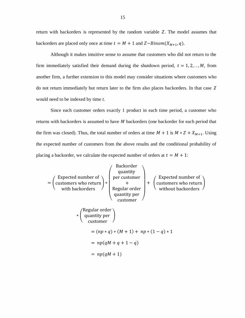
Since each customer orders exactly 1 product in each time period, a customer who

returns with backorders is assumed to have 𝑀 backorders (one backorder for each period that

the firm was closed). Thus, the total number of orders at time 𝑀 + 1 is 𝑀 ∗ 𝑍 + 𝑋𝑀+1. Using

the expected number of customers from the above results and the conditional probability of

placing a backorder, we calculate the expected number of orders at 𝑡 = 𝑀 + 1:

= (Expected number ofcustomers who returnwith backorders

) ∗

(

Backorder quantity

per customer +

Regular order quantity per customer )

+ (Expected number ofcustomers who returnwithout backorders

)

∗ (Regular order quantity per customer

)

= (𝑛𝑝 ∗ 𝑞) ∗ (𝑀 + 1) + 𝑛𝑝 ∗ (1 − 𝑞) ∗ 1

= 𝑛𝑝(𝑞𝑀 + 𝑞 + 1 − 𝑞)

= 𝑛𝑝(𝑞𝑀 + 1)

16

The expected cumulative orders at time 𝑡 = 𝑀 + 𝑖 for 𝑖 > 1 equals 𝑛 (1 − (1 − 𝑝)𝑖), which

is equivalent to the expected cumulative number of customers who have returned by time 𝑡 =

𝑀 + 𝑖.

If the firm’s per-unit selling price is 𝑐, we calculate 𝑅𝑡 the lost revenue at time 𝑡:

𝑅𝑡 =

{

𝑐𝑛 if 𝑡 = 1,2, . . , 𝑀𝑐(𝑛 – 𝑋𝑀+1 − 𝑍) if 𝑡 = 𝑀 + 1

𝑐 (𝑛 – ∑𝑋𝑀+𝑖

𝑡

𝑖=1

) if 𝑡 = 𝑀 + 2,𝑀 + 3,…

The expected lost revenue at time 𝑡 is denoted as �̅�𝑡.

3.3 Production Capacity Considerations

In the proposed model, it is important to look at the production capacity of the firm,

especially at time 𝑡 = 𝑀 + 1, when backorders may be received. The number of orders 𝑀 ∗

𝑍 + 𝑋𝑀+1 must not exceed the available capacity 𝐶. If 𝑀 ∗ 𝑍 + 𝑋𝑀+1 > 𝐶, the excess orders

will be carried forward to the next time period, 𝑡 = 𝑀 + 2, but capacity restrictions require

that 𝑀 ∗ 𝑍 + 𝑋𝑀+1 + 𝑋𝑀+2 ≤ 2𝐶.

Similarly, the firm can estimate and forecast the production capacity levels for future

time periods. Depending on the willingness of customers to wait for the backorder delivery,

the firm needs to prioritize production with the goal of meeting customer needs. If customers

are likely to be lost in case of a late delivery, the firm will have to consider whether it can

temporarily increase its production capacity or other alternatives to meet the spike in demand

due to backorders.

17

4. Illustrative Example

This model can be applied to several situations. For example, a consumer-product

manufacturing firm could face a supply chain disruption forcing it to shut down production.

The firm’s customers could react in different ways. One, a retailer who uses inventory during

this period may come back to the firm immediately with backorders to replace its inventory.

Two, a retailer who temporarily switches to another supplier may decide to come back when

the firm starts producing again. Three, a retailer who switches to another supplier may decide

not to come back when the firm starts producing again. The latter retailer may come back at a

later stage depending on the firm’s performance. By estimating the probability that the retailer

takes any of these actions, the model can account for each of these scenarios.

4.1 Lost revenue with backorders

We illustrate the application of this model to a scenario in which a firm experiences a

supply disruption and must stop production for 𝑀 = 4 periods. Table 2.1 provides values for

the parameters in this example.

Table 2.1. Parameters

Symbol Value

Number of customers or demand per period n 100

Per unit selling price in dollars c 1000

Probability with which customers return in each period p 0.15

Conditional probability of backorder requirement q 0.50

Duration of the disruption in periods M 4

18

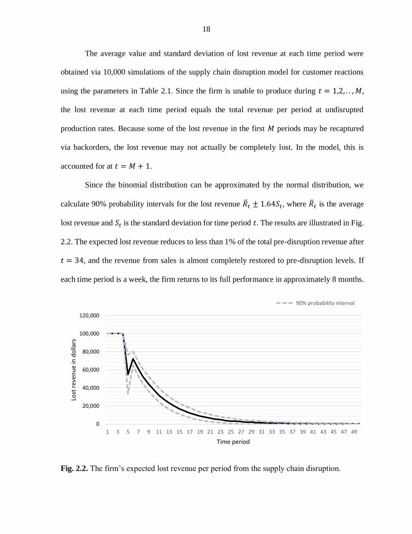
The average value and standard deviation of lost revenue at each time period were

obtained via 10,000 simulations of the supply chain disruption model for customer reactions

using the parameters in Table 2.1. Since the firm is unable to produce during 𝑡 = 1,2, . . , 𝑀,

the lost revenue at each time period equals the total revenue per period at undisrupted

production rates. Because some of the lost revenue in the first 𝑀 periods may be recaptured

via backorders, the lost revenue may not actually be completely lost. In the model, this is

accounted for at 𝑡 = 𝑀 + 1.

Since the binomial distribution can be approximated by the normal distribution, we

calculate 90% probability intervals for the lost revenue �̅�𝑡 ± 1.64𝑆𝑡, where �̅�𝑡 is the average

lost revenue and 𝑆𝑡 is the standard deviation for time period 𝑡. The results are illustrated in Fig.

2.2. The expected lost revenue reduces to less than 1% of the total pre-disruption revenue after

𝑡 = 34, and the revenue from sales is almost completely restored to pre-disruption levels. If

each time period is a week, the firm returns to its full performance in approximately 8 months.

Fig. 2.2. The firm’s expected lost revenue per period from the supply chain disruption.

0

20,000

40,000

60,000

80,000

100,000

120,000

1 3 5 7 9 11 13 15 17 19 21 23 25 27 29 31 33 35 37 39 41 43 45 47 49

Lost

rev

enu

e in

do

llars

Time period

90% probability interval

19

As depicted by the probability interval, there is a 5% probability the lost revenue will

be less than $1,000 within 24 periods and a 5% probability the lost revenue will be greater than

$1,000 for at least 42 time periods. The expected lost revenue is at its maximum value for the

first four periods, which is equal to the total pre-disruption revenue per period and then drops

from $100,000 to $55,000. The downward spike in the expected lost revenue is due to the

backorders. The lost revenue at 𝑡 = 5 has a 5% probability of being as low as $33,444, which

would occur if many customers return with backorders. If very few customers return with

backorders, the lost revenue could be $76,556, which is the 95% upper bound for lost revenue

in that time period. At time 𝑡 = 6, the expected lost revenue increases to $72,250 and then

gradually decreases over time as the firm recovers from the disruption.

4.2 Lost revenue without backorders

Certain disruptions may not allow for backorders. For instance, a restaurant could be

closed for a period of time because of food poisoning, and when it reopens, backorders are not

realistic because the delivered product is a service that cannot be backordered. We can assign

𝑞 = 0 in the simulation model to reflect such a situation. Fig. 2.3 illustrates this scenario

without backorders. Here, the expected cumulative lost revenue is higher because of the lack

of backorders.

20

Fig. 2.3. The firm’s expected lost revenue without backorders.

4.3 Customers with varying demand

The assumption that each customer buys exactly one product may not be valid. This

sub-section extends the simulation model to accommodate varying demands from the firm’s

customers. The demand from customer 𝑙 is 𝑛𝑙 where 𝑙 = 1, 2,… , 𝑛. We assume each 𝑛𝑙 follows

a discrete uniform distribution between 1 and 5, i.e., 𝑛𝑙 ~ 𝑈(1, 5). Backorders are ignored for

simplicity. Parameters from Table 2.1 along with a simulation of 𝑛𝑙 ~ 𝑈(1, 5) were used in the

model with varying demand from different customers to run 1,000 simulations. The results are

illustrated in Fig. 2.4.

The maximum total expected lost revenue is much higher than the previous cases

because the total initial demand is more than in the previous cases. The shape of recovery is

very similar to the model in section 4.1 because each customer returns with the same

probability. The expected lost revenue reduces to less than 1% of the total pre-disruption

0

20,000

40,000

60,000

80,000

100,000

120,000

1 3 5 7 9 11 13 15 17 19 21 23 25 27 29 31 33 35 37 39 41 43 45 47 49

Lost

rev

enu

e in

do

llars

Time period


21

revenue after time period 25. This is comparable to the results from the model in sections 4.1

and 4.2. The results might look different if customers returned with different probabilities. For

example, perhaps customers with more demand from the firm might be more likely to return

because it may be more difficult for these customers to get all of their demand satisfied from

the firm’s competitors.

Fig. 2.4. The firm’s expected lost revenue with varying demand from customers

4.4 Risk management insights

A firm can use this model to understand how parameters impact the firm’s expected

lost revenue. The results discussed are highly sensitive to the value of 𝑝. As illustrated in Fig.

2.5, the firm recovers more quickly when the probability with which customers are gained back

in each period is larger. This makes intuitive sense since firms with loyal customers tend to

recover faster. We observe that the downward spike at time 𝑡 = 𝑀 + 1 is directly correlated

0

50,000

100,000

150,000

200,000

250,000

300,000

350,000

1 3 5 7 9 11 13 15 17 19 21 23 25 27 29 31 33 35 37 39 41 43 45 47 49

Lost

rev

enu

e in

do

llars

Time period


22

with 𝑝. At 𝑡 = 𝑀 + 1, the cumulative expected number of orders including the backorders is

directly proportional to the probability of customers buying from the firm at a given time period

after the disruption.

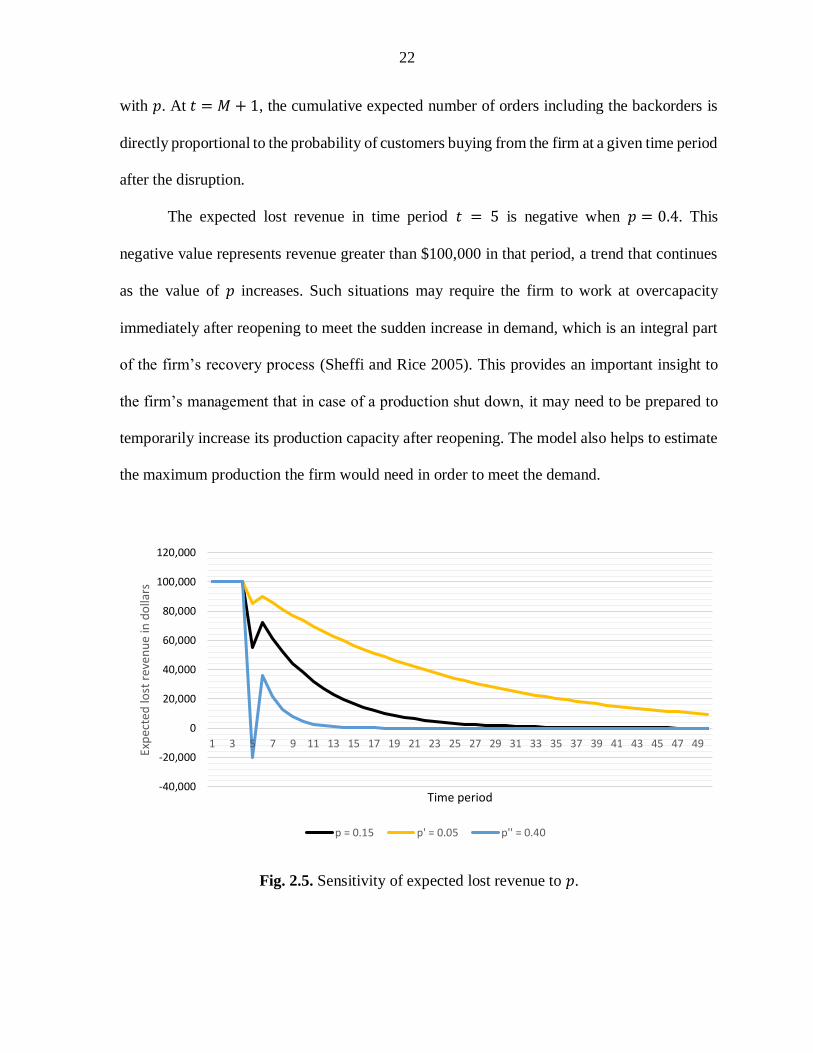
The expected lost revenue in time period 𝑡 = 5 is negative when 𝑝 = 0.4. This

negative value represents revenue greater than $100,000 in that period, a trend that continues

as the value of 𝑝 increases. Such situations may require the firm to work at overcapacity

immediately after reopening to meet the sudden increase in demand, which is an integral part

of the firm’s recovery process (Sheffi and Rice 2005). This provides an important insight to

the firm’s management that in case of a production shut down, it may need to be prepared to

temporarily increase its production capacity after reopening. The model also helps to estimate

the maximum production the firm would need in order to meet the demand.

Fig. 2.5. Sensitivity of expected lost revenue to 𝑝.

-40,000

-20,000

0

20,000

40,000

60,000

80,000

100,000

120,000

1 3 5 7 9 11 13 15 17 19 21 23 25 27 29 31 33 35 37 39 41 43 45 47 49

Exp

ecte

d lo

st r

even

ue

in d

olla

rs

Time period

p = 0.15 p' = 0.05 p'' = 0.40

23

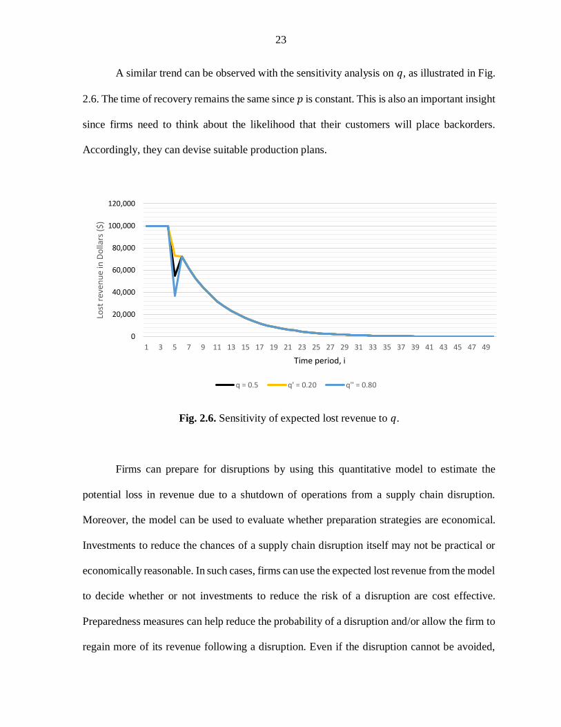
A similar trend can be observed with the sensitivity analysis on 𝑞, as illustrated in Fig.

2.6. The time of recovery remains the same since 𝑝 is constant. This is also an important insight

since firms need to think about the likelihood that their customers will place backorders.

Accordingly, they can devise suitable production plans.

Fig. 2.6. Sensitivity of expected lost revenue to 𝑞.

Firms can prepare for disruptions by using this quantitative model to estimate the

potential loss in revenue due to a shutdown of operations from a supply chain disruption.

Moreover, the model can be used to evaluate whether preparation strategies are economical.

Investments to reduce the chances of a supply chain disruption itself may not be practical or

economically reasonable. In such cases, firms can use the expected lost revenue from the model

to decide whether or not investments to reduce the risk of a disruption are cost effective.

Preparedness measures can help reduce the probability of a disruption and/or allow the firm to

regain more of its revenue following a disruption. Even if the disruption cannot be avoided,

0

20,000

40,000

60,000

80,000

100,000

120,000

1 3 5 7 9 11 13 15 17 19 21 23 25 27 29 31 33 35 37 39 41 43 45 47 49

Lost

rev

enu

e in

Do

llars

($)

Time period, i

q = 0.5 q' = 0.20 q'' = 0.80

24

preparedness measures could reduce the shutdown length 𝑀. It is logical to assume that the

probability of customers returning depends on 𝑀. Decision makers can make decisions about

investing in preparedness measures based on understanding how much revenue will be lost if

the disruption occurs as well as the chances of the disruption itself.

For example, the cumulative expected lost revenue in the illustrative example is

$536,667. A risk-neutral firm should spend at most $536,667 in preparing for this type of

disruption and should spend much less once the probability of a disruption is considered.

Investing in risk reduction strategies such as inventory or an additional supplier could reduce

the time the firm is closed. The chances of customers returning immediately to the firm are

higher if the firm is not closed as long. This would increase the probability p and reduce the

cumulative expected lost revenue. In the example, increasing the value of p from 0.15 to 0.2

decreases the total expected lost revenue from $536,667 to $360,000. Strategies that could

reduce p from 0.15 to 0.2 are economically wise if these strategies cost less than $176,667,

assuming an extremely high probability of disruption.

5. Conclusions

This chapter proposes a model to quantitatively represent the way customers or the

marketplace reacts to a supply chain disruption. The model is used to identify the impact of

such an event on the firm’s revenue. From the firm’s perspective, the total expected lost

revenue is a measure of the impact of the supply chain disruption and can be analyzed to draw

useful insights to manage the risk of such an event.

The results obtained from applying the model serves as an illustration of the usefulness

of the model. The simulation of the customer response model allows the firm to anticipate how

customers might react to a supply chain disruption. The model can inform decision making to

25

manage the risks of a supply chain disruption. Insights from the model can reveal how a

disruption can affect the firm’s revenue depending on the customers’ decisions and the time a

firm takes to recover to its pre-disruption revenue levels. Sensitivity analysis on the model

parameters reveals how the probability at which customers return to the firm impacts the

recovery time. Firms that expect most of its customers to return with backorders may need to

temporarily increase production capacity. Management can use the cumulative expected lost

revenue projections to evaluate investments aimed at increasing the firm’s resilience to supply

chain disruptions.

6. References

Arnade, C., Calvin, L., & Kuchler, F. (2009). Consumer response to a food safety shock: the

2006 food-borne illness outbreak of E. coli O157: H7 linked to spinach. Applied

Economic Perspectives and Policy, 31(4), 734-750.

Babich, V., Burnetas, A. N., & Ritchken, P. H. (2007). Competition and diversification

effects in supply chains with supplier default risk. Manufacturing & Service Operations

Management, 9(2), 123-146.

Beach, R. H., Kuchler, F., Leibtag, E. S., & Zhen, C. (2008). The Effects of Avian Influenza

News on Consumer Purchasing Behavior: A Case Study of Italian Consumers' Retail

Purchases (No. 56477). United States Department of Agriculture, Economic Research

Service.

Chopra, S., & Sodhi, M. S. (2004). Managing risk to avoid supply-chain breakdown. MIT

Sloan Management Review, 46(1), 53.

Christopher, M. (2005). Logistics and Supply Chain Management: Creating Value-Adding

26

Networks (3rd ed.). Harlow, England: Pearson Education.

Ellis, S. C., Henry, R. M., & Shockley, J. (2010). Buyer perceptions of supply disruption

risk: A behavioral view and empirical assessment. Journal of Operations Management,

28(1), 34-46.

Hendricks, K. B., & Singhal, V. R. (2005). Association between supply chain glitches and

operating performance. Management Science, 51(5), 695-711.

Jüttner, U., Peck, H., & Christopher, M. (2003). Supply chain risk management: Outlining an

agenda for future research. International Journal of Logistics: Research and

Applications, 6(4), 197-210.

Kilubi, I., & Haasis, H. D. (2015). Supply chain risk management enablers: A framework

development through systematic review of the literature from 2000 to 2015.

International Journal of Business Science & Applied Management, 10(1), 35-54.

Lavastre, O., Gunasekaran, A., & Spalanzani, A. (2012). Supply chain risk management in

French companies. Decision Support Systems, 52(4), 828-838.

MacKenzie, C. A., Barker, K., & Santos, J. R. (2014). Modeling a severe supply chain

disruption and post-disaster decision making with application to the Japanese

earthquake and tsunami. IIE Transactions, 46(12), 1243-1260.

MacKenzie, C. A., Santos, J. R., & Barker, K. (2012). Measuring changes in international

production from a disruption: Case study of the Japanese earthquake and tsunami.

International Journal of Production Economics, 138(2), 293-302.

Manuj, I., Dittmann, P., & Gaudenzi, B. (2007). Risk management. In J. T. Mentzer, M. B.

Myers, & T. P. Stank (Eds.), Handbook of Global Supply Chain Management (pp.

319-336). Thousand Oaks, Calif.: Sage Publications.

27

Mentzer, J. T., DeWitt, W., Keebler, J. S., Min, S., Nix, N. W., Smith, C. D., & Zacharia, Z.

G. (2001). Defining supply chain management. Journal of Business Logistics, 22(2),

1-25.

Nagurney, A., Cruz, J., Dong, J., & Zhang, D. (2005). Supply chain networks, electronic

commerce, and supply side and demand side risk. European Journal of Operational

Research, 164(1), 120-142.

Nishat Faisal, M., Banwet, D. K., & Shankar, R. (2006). Mapping supply chains on risk and

customer sensitivity dimensions. Industrial Management & Data Systems, 106(6), 878-

895.

Sheffi, Y., & Rice Jr, J. B. (2005). A supply chain view of the resilient enterprise. MIT Sloan

Management Review, 47(1), 41.

Snyder, L. V., Atan, Z., Peng, P., Rong, Y., Schmitt, A. J., & Sinsoysal, B. (2016). OR/MS

models for supply chain disruptions: A review. IIE Transactions, 48(2), 89-109.

Sodhi, M. S., & Tang, C. S. (2012). Managing Supply Chain Risk. New York: Springer

Science & Business Media.

Stecke, K. E., & Kumar, S. (2009). Sources of supply chain disruptions, factors that breed

vulnerability, and mitigating strategies. Journal of Marketing Channels, 16(3), 193-226.

Tomlin, B., & Wang, Y. (2005). On the value of mix flexibility and dual sourcing in

unreliable newsvendor networks. Manufacturing & Service Operations Management,

7(1), 37-57.

Xia, Y., Ramachandran, K., & Gurnani, H. (2011). Sharing demand and supply risk in a

supply chain. IIE Transactions, 43(6), 451-469.

Yu, H., Zeng, A. Z., & Zhao, L. (2009). Single or dual sourcing: Decision-making in the

28

presence of supply chain disruption risks. Omega, 37(4), 788-800.

29

CHAPTER 3. COST-EFFECTIVENESS ANALYSIS OF SUPPLIER

PERFORMANCE BASED ON SCOR METRICS

Based on an abstract accepted for presentation at the 2017 IISE Annual Conference

Arun Vinayak, Cameron A. MacKenzie

Abstract

A firm may use several metrics to assess a supplier’s performance, including the quality of

delivered products, the time it takes to deliver those products, and how quickly a supplier

responds to changes in customer demand. Mapping these measures to what a firm ultimately

cares about can help a firm select among suppliers. If a firm has little to no experience working

with a supplier, a firm may have difficulty in objectively selecting a supplier. This paper

presents a framework for supplier performance measurement based on supplier key

performance indicators derived from the performance metrics of the Supply Chain Operations

Reference model. The framework can be used for supplier selection as well as for supplier

performance monitoring as the firm continues to work with the selected supplier. A decision

maker in a firm can incorporate his or her own preferences within the presented framework to

determine the most preferred supplier and assess the cost effectiveness.

Keywords: Supplier performance evaluation, SCOR model, Multi-objective decision making,

Risk analysis, Supply chain.

30

3.1. Introduction

Selecting and evaluating a supplier is a multi-criteria problem that is growing in its

scope and importance (Ho et al., 2010; Agarwal et al., 2011). With the availability of latest

technology that can be used to monitor, measure, and compare various aspects of a supplier,

organizations can benefit from a simple and effective framework for supplier selection using

multi-criteria decision-making techniques. Emphasis on the firm’s objectives and business

requirements while selecting a supplier will play a critical role in the success of any firm as

there is an increased dependency on suppliers due to business initiatives such as outsourcing,

globalization, and lean manufacturing. While such focus on the firm’s core values is vital, an

effective supplier performance benchmarking framework must be simple and standardized for

the use of multiple industries.

The Supply Chain Operations References (SCOR) model developed by the Supply

Chain Council (SCC) with inputs from industry leaders presents a comprehensive hierarchical

structure of a supply chain’s performance metrics under five core performance attributes:

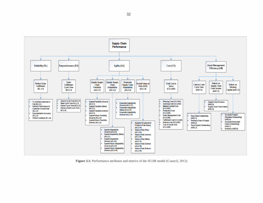
reliability, responsiveness, agility, cost, and asset management efficiency. Fig. 3.1 presents the

hierarchy of metrics of levels 1 and 2 for these five core attributes. To ensure balanced decision

making in supply chain management, the SCC suggests that supply chain scorecards should

contain at least one metric for each performance attribute. Although these five core

performance attributes may be mutually exclusive, they are not directly measurable. There are

43 level-1 performance metrics that support these five attributes which would require extensive

data gathering and is not practical. Moreover, these metrics in the SCOR model are designed

to measure a supply chain’s performance. While SCOR model serves as a comprehensive

31

reference guide for supply chain performance measurement, there is a need for deriving a set

of metrics that most effectively captures the performance of a supplier.

This paper presents a practical tool that simplifies and combines these attributes to

account for their relative importance using a systematic process. Key Performance Indicators

(KPIs) for the suppliers derived from the SCOR performance metrics enable us to compare

different suppliers from a firm’s perspective and understand the risk associated with them. A

subset of the SCOR performance metrics are identified and then aggregated using a value-

based approach to multi-criteria decision making. An Excel-based tool is presented for decision

makers from a firm to incorporate their own preferences for carefully evaluating and

identifying the best supplier in a rational mode. An illustrative case application of the proposed

framework based on real world expertise is also presented that can be referred by analysts or

decision makers from the industry to apply the framework in selecting new suppliers or

evaluating existing suppliers.

32

Figure 3.1: Performance attributes and metrics of the SCOR model (Council, 2012)

33

The model adapts the SCOR metrics for reliability, responsiveness, agility, and asset

management efficiency by focusing on the most important metrics and constructing a value

function based on those metrics. The value function aggregates the attributes into a single

measure of effectiveness. The cost of the supplier is separated from the effectiveness measure

in order to make trade-offs between the cost and effectiveness of suppliers. Since several of

the SCOR metrics concern evaluating activities for material flow, the proposed model is

intended for manufacturing supply chains.

This paper is organized as follows: a literature review is given in Section 3.2. Section

3.3 presents the model framework along with an overview of the SCOR performance metrics

that serve as the basis of the supplier KPIs presented in this paper. Section 3.4 describes an

illustrative example. Section 3.5 concludes the paper with recommendations, insights, and

conclusions drawn from the study.

3.2. Literature Review

Supplier selection has received significant attention in the academia over the past few

decades. Moore (2014) defines supplier selection as the process through which firms identify,

evaluate and contract with suppliers. Lil (2007) argues that the sole purpose of selection is not

to identify suppliers with the lowest prices and the materials at the right time. Rather, the

process revolves around all strategic decisions aimed at meeting the company’s long-term

goals with less risk. This ensures that selecting the right suppliers dramatically minimizes

purchasing costs while at the same time improving corporate competitiveness. Companies pay

attention to the product life cycle, advanced manufacturing process, and the complexity of the

34

design and manufacturing process when making supplier selection decisions (Mohammady &

Martinez, 2006). Buyers are concerned with the supplier’s willingness to deliver the right

quality at the right time, mutual trust between buyer and seller, and the seller’s technical and

financial capabilities (Lima-Junior & Carpinetti. 2016).

Based on literature review on multi-criteria decision making techniques in 78 journal

papers for supplier evaluation and selection from 2000 to 2008, Ho et al. (2010) identifies Data

Envelopment Analysis (DEA) as the most popular approach. Agarwal et al. (2011) also

identifies DEA as the most widely applied methodology for supplier selection based on 60

articles from various journals and conferences from 2000 to 2011. DEA is robust approach that

mainly focuses on system efficiency and considers suppliers and processes as a system. In

DEA, optimal weights to maximize the efficiency or performance rating of a supplier is

calculated using the outputs (e.g. delivery performance, quality, etc.) and inputs (costs).

Researchers (Weber, 1996; Braglia & Petroni, 2000; Songhori et al., 2011) conclude that

significant benefits to a firm such as reductions in costs, time, and quality can be achieved if

inefficient vendors can become DEA efficient. Moreover, supplier selection itself can be

carried out based on DEA efficiency of available suppliers. Ho et al. (2010) argue that suppliers

can easily get confused by its input and output criteria. The linear programming nature of DEA

also assumes that the most effective suppliers are those that are able generate more outputs by

using less inputs (Murkherjee, 2017). This is one of the main disadvantages of using DEA (Ho

et al., 2010).

On the other hand, based on a review of multi-criteria decision making approaches for

green supplier selection in literature from 1997 to 2011, Govindan et al., (2013) concludes that

Analytical Hierarchy Process (AHP), a less data intensive and structured method for multi-

35

objective decisions, is the most widely used approach. Basnet (2002) points that unlike other

methods, AHP is easy to use, highly flexible and can be used in a wide range of fields.

Furthermore, the method can be used to make a consistent decision with respect to multiple

qualitative and quantitative criteria (Huan, Sheoran &Wang, 2004). Suppliers could use the

combined approach of AHP and Quality Function Deployment (QFD), a management tool that

provides a visual connective process to help teams focus on the needs of the customers

throughout the total development cycle of a product or process (Moore, 2014; Bouchereau &

Rowlands, 2000). When using this combination, the best supplier is assumed to be one that can

efficiently meet most of the buyer requirements (Basnet, 2002). The QFD model is similar to

the Simple Multi-attribute Rating Technique (SMART) which helps major decision-makers in

the purchasing company to account for factors that are both qualitative and quantitative (Ho et

al. 2010). Unlike QFD, the SMART model can structure the supplier’s system and the

environment into components that interact with each other to measure and regulate various

effects of system errors.

The SCOR model is one of the most promising models for supply chain strategic

decision making (Ravindran, 2013). Established in 1996, the model is a re-engineering,

benchmarking, process measurement and best practice analysis to be used in supply chain as

an integral modelling. SCOR works on the principle of aligning supply chain management

practices as well as filling the gaps in supply chain (Lima-Junior and Carpinetti, 2016). Also,

the model strives to improve the use of network modelling tools to support management

decision and can be integrated with multi-criteria decision-making techniques. Due to this

reason researchers agree the SCOR model remains the most effective individualized approach

of supplier chain performance measurement given that it can produce better results on its own,

36

compared to other models (Huang & Keskar, 2007; Huan et al., 2004; Kocaoğlu et al., 2013;

Lima-Junior et al., 2016).

Integrated and individualized supplier selection methods are significant as they aid

suppliers to select the most suitable and efficient suppliers. Using supplier selection methods

ensures that companies get to work with the best suppliers who can effectively meet their

specific demands. Supplier efficiency not only focuses on cost and ability to deliver quality

goods at the right time but also on other equally important factors such as trust, financial

capability and supplier’s past reputation. However, there is a lack of alignment in the existing

literature between supplier selection and supply chain strategic decision making as researchers

overly emphasized the use of quantitative optimization models in supplier selection (Huang &

Keskar, 2007). Hence, there is a pressing need for researchers to fill this gap. Firms should

evaluate the expected level of supplier performance along with cost before selecting the most

suitable one.

Lastly, there is a need to introduce more models that use value-focused multi-criteria

decision-making techniques to address the problem of supplier selection. This is because the

technique can integrate the supplier’s structure and capabilities with the requirement of a firm.

In the existing literature in supplier selection, methods such as DEA are chosen over value-

based techniques since the latter requires more involvement of the decision maker (Seydel

2006). But from a practical perspective, identifying the right objectives and KPIs with the

involvement of the decision makers is most important to a firm when compared to

computationally intelligent methods to optimize supplier selection. The objective of this

chapter is to improve the quality of supplier selection process in the industry by presenting a

framework, based on existing multi-criteria decision-making techniques, that provides insights

37

on the trade-offs, increases confidence (or highlight the risk) in the decision, and document the

process. The presented framework can be potentially used by firms to evaluate new suppliers

using their supplier selection phase with the easy to use Excel tool.

3.3. Methodology

This section defines a framework to help a firm select a supplier. The framework is

based on the SCOR model which proposes a set of 43 metrics. The SCOR model provides a

framework from which to construct a multi-criteria value model that aggregates these metrics

into a single number that describes the effectiveness of a supplier. This section reviews the

SCOR performance metrics, translates the SCOR model to an objectives hierarchy, and

describes the value functions and weights needed to quantify supplier effectiveness.

3.3.1 Overview of SCOR Performance Metrics

The SCOR model, first developed by the SCC in 1996, is a very promising model for supply

chain strategic decision making (Huan et al., 2004). It allows firms to perform a very thorough

fact-based analysis of all aspects of their supply chain by providing a complete set of process

details, performance metrics, and industry best practices. SCOR identifies five core supply

chain performance attributes with 10 level-1 or strategic metrics and 43 level-2 metrics as

shown in Fig. 3.1. Below is a summary of the SCOR performance metrics as defined by the

Supply Chain Council in SCOR model reference documentation revision 11.0:

• Reliability: Reliability describes the ability to perform tasks as expected. This attribute

focuses on predicting the outcome of a process. The level-1 metric associated with

reliability is perfect order fulfilment, which can be defined as the percentage of orders

38

meeting delivery performance with complete and accurate documentation and no delivery

damage. Perfect order fulfilment is further broken down into: percentage of orders

delivered in full, delivery performance to customer commit date, documentation accuracy,

and perfect condition.

• Responsiveness: Responsiveness describes the speed at which tasks are performed in a

supply chain. This is measured by the order fulfillment cycle time, which is the average

cycle time to fulfil customer orders. The order fulfillment cycle time is composed of cycle

times for the source, make, deliver, and delivery retail.

• Agility: Agility describes the ability of a supply chain to respond to marketplace changes

to gain or maintain competitive advantage. The three level-1 metrics associated with agility

are: Upside supply chain flexibility is the amount of time it takes a supply chain to respond

to an unplanned 20 percent increase in demand without service or cost penalty. Upside

supply chain adaptability is the quantity of increased production a supply chain can achieve

and sustain for 30 days. Downside supply chain adaptability is the reduction in order

quantities sustainable at 30 days prior to delivery with no inventory or cost penalties. Value

at risk is a popular risk metric widely used by the finance industry to understand the risk

exposure of a trading portfolio based on historic volatility.

• Cost: In the context of supply chain performance measurement, SCOR model describes

cost as the operational costs of various processes in a supply chain. This is an internally

focused attribute that is measured by the total cost to serve in monetary unites as a sum of

planning cost, sourcing cost, material landed cost, production cost, order management cost,

fulfillment cost, and returns cost.

39

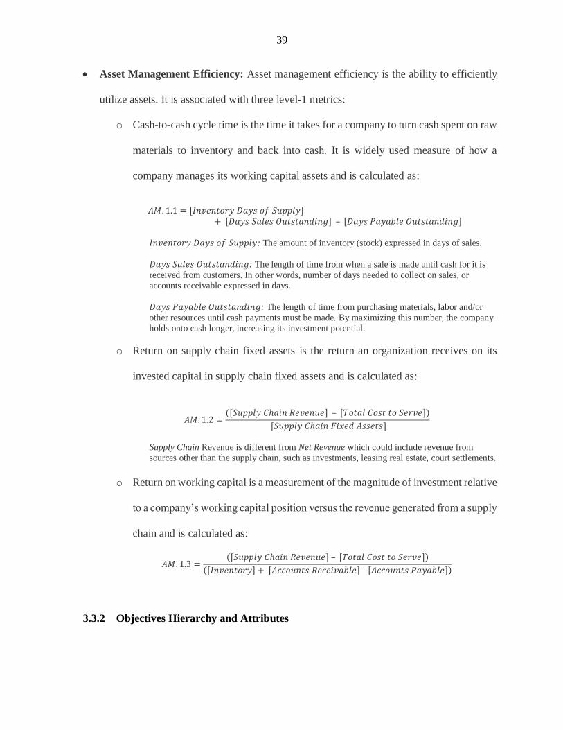
• Asset Management Efficiency: Asset management efficiency is the ability to efficiently

utilize assets. It is associated with three level-1 metrics:

o Cash-to-cash cycle time is the time it takes for a company to turn cash spent on raw

materials to inventory and back into cash. It is widely used measure of how a

company manages its working capital assets and is calculated as:

𝐴𝑀. 1.1 = [𝐼𝑛𝑣𝑒𝑛𝑡𝑜𝑟𝑦 𝐷𝑎𝑦𝑠 𝑜𝑓 𝑆𝑢𝑝𝑝𝑙𝑦] + [𝐷𝑎𝑦𝑠 𝑆𝑎𝑙𝑒𝑠 𝑂𝑢𝑡𝑠𝑡𝑎𝑛𝑑𝑖𝑛𝑔] – [𝐷𝑎𝑦𝑠 𝑃𝑎𝑦𝑎𝑏𝑙𝑒 𝑂𝑢𝑡𝑠𝑡𝑎𝑛𝑑𝑖𝑛𝑔]

𝐼𝑛𝑣𝑒𝑛𝑡𝑜𝑟𝑦 𝐷𝑎𝑦𝑠 𝑜𝑓 𝑆𝑢𝑝𝑝𝑙𝑦: The amount of inventory (stock) expressed in days of sales.

𝐷𝑎𝑦𝑠 𝑆𝑎𝑙𝑒𝑠 𝑂𝑢𝑡𝑠𝑡𝑎𝑛𝑑𝑖𝑛𝑔: The length of time from when a sale is made until cash for it is

received from customers. In other words, number of days needed to collect on sales, or

accounts receivable expressed in days.

𝐷𝑎𝑦𝑠 𝑃𝑎𝑦𝑎𝑏𝑙𝑒 𝑂𝑢𝑡𝑠𝑡𝑎𝑛𝑑𝑖𝑛𝑔: The length of time from purchasing materials, labor and/or

other resources until cash payments must be made. By maximizing this number, the company

holds onto cash longer, increasing its investment potential.

o Return on supply chain fixed assets is the return an organization receives on its

invested capital in supply chain fixed assets and is calculated as:

𝐴𝑀. 1.2 =([𝑆𝑢𝑝𝑝𝑙𝑦 𝐶ℎ𝑎𝑖𝑛 𝑅𝑒𝑣𝑒𝑛𝑢𝑒] – [𝑇𝑜𝑡𝑎𝑙 𝐶𝑜𝑠𝑡 𝑡𝑜 𝑆𝑒𝑟𝑣𝑒])

[𝑆𝑢𝑝𝑝𝑙𝑦 𝐶ℎ𝑎𝑖𝑛 𝐹𝑖𝑥𝑒𝑑 𝐴𝑠𝑠𝑒𝑡𝑠]

Supply Chain Revenue is different from Net Revenue which could include revenue from

sources other than the supply chain, such as investments, leasing real estate, court settlements.

o Return on working capital is a measurement of the magnitude of investment relative

to a company’s working capital position versus the revenue generated from a supply

chain and is calculated as:

𝐴𝑀. 1.3 =([𝑆𝑢𝑝𝑝𝑙𝑦 𝐶ℎ𝑎𝑖𝑛 𝑅𝑒𝑣𝑒𝑛𝑢𝑒] – [𝑇𝑜𝑡𝑎𝑙 𝐶𝑜𝑠𝑡 𝑡𝑜 𝑆𝑒𝑟𝑣𝑒])

([𝐼𝑛𝑣𝑒𝑛𝑡𝑜𝑟𝑦] + [𝐴𝑐𝑐𝑜𝑢𝑛𝑡𝑠 𝑅𝑒𝑐𝑒𝑖𝑣𝑎𝑏𝑙𝑒]– [𝐴𝑐𝑐𝑜𝑢𝑛𝑡𝑠 𝑃𝑎𝑦𝑎𝑏𝑙𝑒])

3.3.2 Objectives Hierarchy and Attributes

40

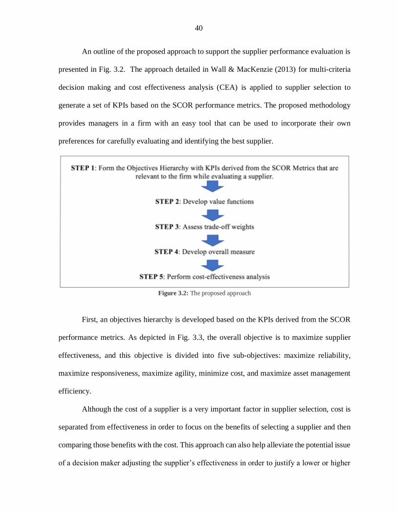
An outline of the proposed approach to support the supplier performance evaluation is

presented in Fig. 3.2. The approach detailed in Wall & MacKenzie (2013) for multi-criteria

decision making and cost effectiveness analysis (CEA) is applied to supplier selection to

generate a set of KPIs based on the SCOR performance metrics. The proposed methodology

provides managers in a firm with an easy tool that can be used to incorporate their own

preferences for carefully evaluating and identifying the best supplier.

Figure 3.2: The proposed approach

First, an objectives hierarchy is developed based on the KPIs derived from the SCOR

performance metrics. As depicted in Fig. 3.3, the overall objective is to maximize supplier

effectiveness, and this objective is divided into five sub-objectives: maximize reliability,

maximize responsiveness, maximize agility, minimize cost, and maximize asset management

efficiency.

Although the cost of a supplier is a very important factor in supplier selection, cost is

separated from effectiveness in order to focus on the benefits of selecting a supplier and then

comparing those benefits with the cost. This approach can also help alleviate the potential issue

of a decision maker adjusting the supplier’s effectiveness in order to justify a lower or higher

41

cost (Williams & Thompson, 2004). Cost is defined as the total cost associated with doing

business with a supplier. Cost is excluded from the objectives hierarchy and considered in the

final step of the methodology for CEA.

We identify 13 attributes based on the SCOR performance metrics (Fig. 3.4). The

presented methodology is generic and the objectives hierarchy can be modified with other KPIs

derived from the SCOR model depending on the firm or the industry. The selected indicators

for the framework presented in this paper are shown in Table 3.1. As for the definition of KPIs,

the SCOR model has provided with complete definitions for references in the context of an

overall supply chain. However, to suit the context of supplier selection as opposed to supply

chain performance evaluation, new definitions for the metrics or KPIs are presented in Table

3.1. During the application of this framework, these definitions could be altered based on

interviews and discussion with management and staff of the case company. During the process

of supplier selection, the KPIs and their definitions (after any necessary alterations) must be

sent to each of the suppliers under consideration so that they can submit their estimated KPI

values based on their capabilities.

42

Figure 3.3: Objectives hierarchy for supplier effectiveness

43

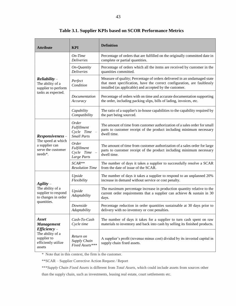
Table 3.1. Supplier KPIs based on SCOR Performance Metrics

Attribute

KPI

Definition

Reliability –

The ability of a

supplier to perform

tasks as expected.

On-Time

Deliveries

Percentage of orders that are fulfilled on the originally committed date in

complete or partial quantities.

On-Quantity

Deliveries

Percentage of orders which all the items are received by customer in the

quantities committed.

Perfect

Condition

Measure of quality; Percentage of orders delivered in an undamaged state

that meet specification, have the correct configuration, are faultlessly

installed (as applicable) and accepted by the customer.

Documentation

Accuracy

Percentage of orders with on time and accurate documentation supporting

the order, including packing slips, bills of lading, invoices, etc.

Capability

Compatibility

The ratio of a supplier's in-house capabilities to the capability required by

the part being sourced.

Responsiveness –

The speed at which

a supplier can

serve the customer

needs*.

Order

Fulfillment

Cycle Time –

Small Parts

The amount of time from customer authorization of a sales order for small

parts to customer receipt of the product including minimum necessary

dwell time.

Order

Fulfillment

Cycle Time –

Large Parts

The amount of time from customer authorization of a sales order for large

parts to customer receipt of the product including minimum necessary

dwell time.

SCAR**

Resolution Time

The number of days it takes a supplier to successfully resolve a SCAR

from the date of issue of the SCAR.

Agility – The ability of a

supplier to respond

to changes in order

quantities.

Upside

Flexibility

The number of days it takes a supplier to respond to an unplanned 20%

increase in demand without service or cost penalty.

Upside

Adaptability

The maximum percentage increase in production quantity relative to the

current order requirements that a supplier can achieve & sustain in 30

days.

Downside

Adaptability

Percentage reduction in order quantities sustainable at 30 days prior to

delivery with no inventory or cost penalties.

Asset

Management

Efficiency – The ability of a

supplier to

efficiently utilize

assets

Cash-To-Cash

Cycle time

The number of days it takes for a supplier to turn cash spent on raw

materials to inventory and back into cash by selling its finished products.

Return on

Supply Chain

Fixed Assets***

A supplier’s profit (revenue minus cost) divided by its invested capital in

supply chain fixed assets.

* Note that in this context, the firm is the customer.

**SCAR – Supplier Corrective Action Request / Report

***Supply Chain Fixed Assets is different from Total Assets, which could include assets from sources other

than the supply chain, such as investments, leasing real estate, court settlements etc.

44

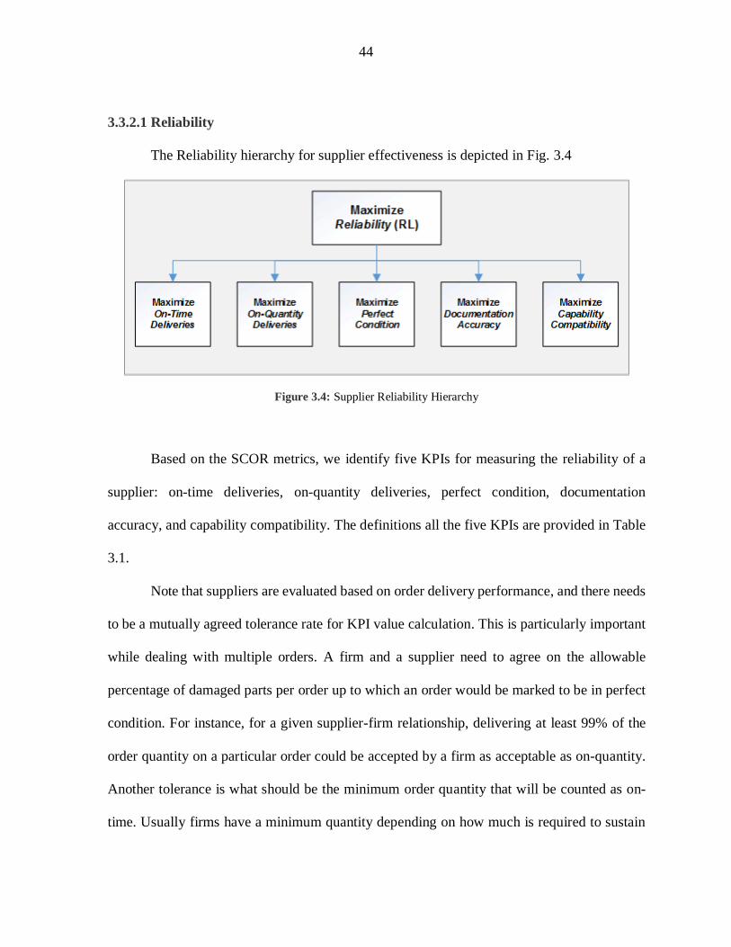
3.3.2.1 Reliability

The Reliability hierarchy for supplier effectiveness is depicted in Fig. 3.4

Figure 3.4: Supplier Reliability Hierarchy

Based on the SCOR metrics, we identify five KPIs for measuring the reliability of a

supplier: on-time deliveries, on-quantity deliveries, perfect condition, documentation

accuracy, and capability compatibility. The definitions all the five KPIs are provided in Table

3.1.

Note that suppliers are evaluated based on order delivery performance, and there needs

to be a mutually agreed tolerance rate for KPI value calculation. This is particularly important

while dealing with multiple orders. A firm and a supplier need to agree on the allowable

percentage of damaged parts per order up to which an order would be marked to be in perfect

condition. For instance, for a given supplier-firm relationship, delivering at least 99% of the

order quantity on a particular order could be accepted by a firm as acceptable as on-quantity.

Another tolerance is what should be the minimum order quantity that will be counted as on-

time. Usually firms have a minimum quantity depending on how much is required to sustain

45

production until they receive their next shipment to complete the order. Also, one might argue

that the KPIs on-time and on-quantity measures the same. But with only one KPI for measuring

on-time and on-quantity deliveries, suppliers will not have any incentive to deliver partial

shipments when on-quantity deliveries are not possible. Failure to receive any orders on the

committed date could affect the operations of a firm significantly and hence having a KPI for

on-time delivery becomes important in such scenarios. In the context of a new supplier, a firm

can ask a supplier to provide estimates based on their business capabilities and historic

performance.

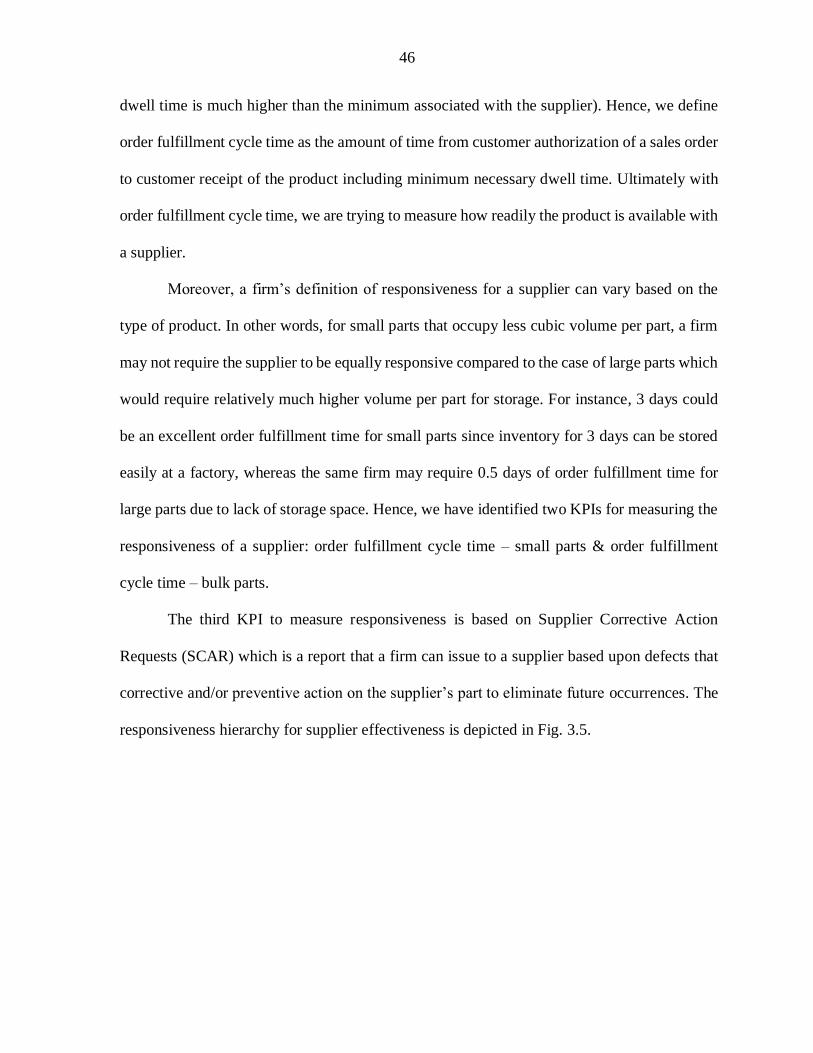
3.3.2.2 Responsiveness

Order fulfillment cycle time can be defined as the total cycle time from the order

placement by the customer to the acceptance of the order by the customer. This includes all

the time between these two events irrespective of whether the supplier was fulfilling the order.

It could be the case that the customer placed the order in advance to reserve capacity or

material. Hence, order fulfillment cycle time consist of two components: order fulfillment

process time and dwell time. Note that the components of order fulfillment process time will

depend on the supplier’s business model. For instance, for a supplier with a make-to-stock

business model, it would include only order processing and transportation time whereas for a

supplier with make-to-order and it would also include the manufacturing time. Even though

order fulfillment process time most accurately reflects the responsiveness of an organization,

one can make the argument that if a supplier has too many customers lined up, the dwell time

is significant to measuring the responsiveness of a supplier. But at the same time, a supplier’s

responsiveness should not be impacted by orders that are placed much earlier in time (where

46

dwell time is much higher than the minimum associated with the supplier). Hence, we define

order fulfillment cycle time as the amount of time from customer authorization of a sales order

to customer receipt of the product including minimum necessary dwell time. Ultimately with

order fulfillment cycle time, we are trying to measure how readily the product is available with

a supplier.

Moreover, a firm’s definition of responsiveness for a supplier can vary based on the

type of product. In other words, for small parts that occupy less cubic volume per part, a firm

may not require the supplier to be equally responsive compared to the case of large parts which

would require relatively much higher volume per part for storage. For instance, 3 days could

be an excellent order fulfillment time for small parts since inventory for 3 days can be stored

easily at a factory, whereas the same firm may require 0.5 days of order fulfillment time for

large parts due to lack of storage space. Hence, we have identified two KPIs for measuring the

responsiveness of a supplier: order fulfillment cycle time – small parts & order fulfillment

cycle time – bulk parts.

The third KPI to measure responsiveness is based on Supplier Corrective Action

Requests (SCAR) which is a report that a firm can issue to a supplier based upon defects that

corrective and/or preventive action on the supplier’s part to eliminate future occurrences. The

responsiveness hierarchy for supplier effectiveness is depicted in Fig. 3.5.

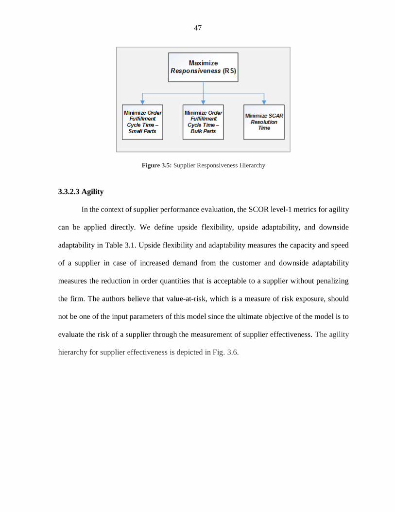
47

Figure 3.5: Supplier Responsiveness Hierarchy

3.3.2.3 Agility

In the context of supplier performance evaluation, the SCOR level-1 metrics for agility

can be applied directly. We define upside flexibility, upside adaptability, and downside

adaptability in Table 3.1. Upside flexibility and adaptability measures the capacity and speed

of a supplier in case of increased demand from the customer and downside adaptability

measures the reduction in order quantities that is acceptable to a supplier without penalizing

the firm. The authors believe that value-at-risk, which is a measure of risk exposure, should

not be one of the input parameters of this model since the ultimate objective of the model is to

evaluate the risk of a supplier through the measurement of supplier effectiveness. The agility

hierarchy for supplier effectiveness is depicted in Fig. 3.6.

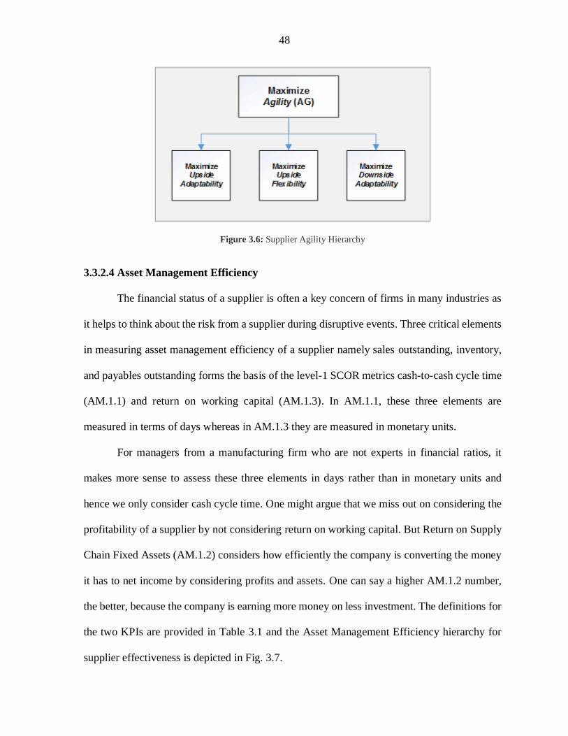
48

Figure 3.6: Supplier Agility Hierarchy

3.3.2.4 Asset Management Efficiency

The financial status of a supplier is often a key concern of firms in many industries as

it helps to think about the risk from a supplier during disruptive events. Three critical elements

in measuring asset management efficiency of a supplier namely sales outstanding, inventory,

and payables outstanding forms the basis of the level-1 SCOR metrics cash-to-cash cycle time

(AM.1.1) and return on working capital (AM.1.3). In AM.1.1, these three elements are

measured in terms of days whereas in AM.1.3 they are measured in monetary units.

For managers from a manufacturing firm who are not experts in financial ratios, it

makes more sense to assess these three elements in days rather than in monetary units and

hence we only consider cash cycle time. One might argue that we miss out on considering the

profitability of a supplier by not considering return on working capital. But Return on Supply

Chain Fixed Assets (AM.1.2) considers how efficiently the company is converting the money

it has to net income by considering profits and assets. One can say a higher AM.1.2 number,

the better, because the company is earning more money on less investment. The definitions for

the two KPIs are provided in Table 3.1 and the Asset Management Efficiency hierarchy for

supplier effectiveness is depicted in Fig. 3.7.

49

Figure 3.7: Supplier Asset Management Efficiency Hierarchy

With the measurable KPIs that form the bottom level of the objectives hierarchy, an

additive value function can be used to measure the effectiveness of a supplier (Kirkwood

1997). This framework assumes preferential independence of the KPIs. The additive value

function is comprised of an individual value function for each KPI and swing weights that

describe the trade-offs between the KPIs and objectives.

3.3.3 Value Functions: Marginal Preferences in KPI values

The second step of the proposed framework uses value functions to convert a decision

maker’s preferences to real number under conditions of certainty. Value functions are most

appropriate when there are multiple and conflicting objectives, and the attributes do not have

any uncertainty. We consider a deterministic case in which no uncertainty is associated with

the supplier KPIs. Assessing value functions require interpersonal communication between an

analyst and a decision maker and can be done using several methods. The direct rating method

directly assigns values to various levels of a criterion and is most useful when the metric has a

few discrete levels. In the mid-value splitting technique, a value function is developed based

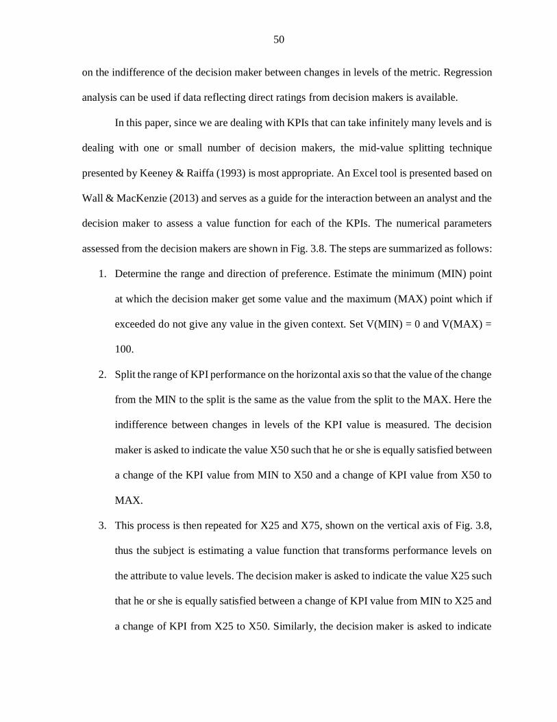
50

on the indifference of the decision maker between changes in levels of the metric. Regression

analysis can be used if data reflecting direct ratings from decision makers is available.

In this paper, since we are dealing with KPIs that can take infinitely many levels and is

dealing with one or small number of decision makers, the mid-value splitting technique

presented by Keeney & Raiffa (1993) is most appropriate. An Excel tool is presented based on

Wall & MacKenzie (2013) and serves as a guide for the interaction between an analyst and the

decision maker to assess a value function for each of the KPIs. The numerical parameters

assessed from the decision makers are shown in Fig. 3.8. The steps are summarized as follows:

1. Determine the range and direction of preference. Estimate the minimum (MIN) point

at which the decision maker get some value and the maximum (MAX) point which if

exceeded do not give any value in the given context. Set V(MIN) = 0 and V(MAX) =

100.

2. Split the range of KPI performance on the horizontal axis so that the value of the change

from the MIN to the split is the same as the value from the split to the MAX. Here the

indifference between changes in levels of the KPI value is measured. The decision

maker is asked to indicate the value X50 such that he or she is equally satisfied between

a change of the KPI value from MIN to X50 and a change of KPI value from X50 to

MAX.

3. This process is then repeated for X25 and X75, shown on the vertical axis of Fig. 3.8,

thus the subject is estimating a value function that transforms performance levels on

the attribute to value levels. The decision maker is asked to indicate the value X25 such

that he or she is equally satisfied between a change of KPI value from MIN to X25 and

a change of KPI from X25 to X50. Similarly, the decision maker is asked to indicate

51

the value X75 such that he or she is equally satisfied between a change of KPI value

from X50 to X75 and a change of KPI from X75 to MAX.

4. Consistency check: Determine whether there is equal satisfaction with the KPI value

change from X25 to X50 as with a change from X50 to X75. If the answer is

affirmative, the value function can be considered consistent. Otherwise, the decision

maker is asked to revise his or her responses (i.e., steps 1 to 3 are repeated).

Figure 3.8: Mid-value splitting

Using the values obtained, the value functions for each of the KPIs in the objectives hierarchy

can be constructed using the Excel tool as explained in Appendix A.

3.3.4 Weights: Making trade-offs between KPIs

MIN

X25

X50

X75

MAX

0.00

0.25

0.50

0.75

1.00

0 10 20 30 40 50 60 70 80 90 100

ValueScale(0-1)

MeasurementScale(x)

On-QuantityDeliveries(%)

ValueFunction Mid-Values Poly.(ValueFunction)

52

A firm with four fundamental objectives may not be able to maximize all four without

making some trade-offs. This framework provides a systematic method for a decision maker

to articulate his or her preference for one objective versus another objective. If the attributes

have uncertainty, the problem becomes more complex because the decision maker needs to

trade-off between objectives under uncertainty.

The weights serve as the decision maker’s reflection of the relative importance of

various criteria. Trade-offs in multi-objective decision making problems are dependent on the

subjective judgement of the decision maker and can vary from one decision maker to the other.

These weights can be assessed using many techniques such as direct assessment, equal

importance, rank sum, rank reciprocal, pairwise comparison, and swing weighting (Wall &

MacKenzie, 2013). In the proposed methodology, the swing weight procedure is used to assess

local trade-off weights. It incorporates ordinal, relative importance, and range of variation of

individual KPIs and involves four major assessment steps as summarized below:

1. A decision maker is presented with a hypothetical supplier in which all the KPI values

within one of the four attributes at their worst or least-preferred values.

2. The KPI for which it is most preferred to change (or swing) from its worst or least-

preferred value to its best or most-preferred value, all other KPIs remaining at their

worst values, is determined.

3. After the first KPI is selected, the decision maker is asked to select the second KPI that

he or she would next choose to move to its best level. The process is repeated for all

KPIs under the selected attribute and the KPIs are ranked from most important to least

important according to the user’s preference.

53

4. A weight of 100 is assigned to the most preferred KPI. Weights to the remaining KPIs

are determined in proportion to their rank of importance.

It is more effective to perform the swing weight method to each objective separately.

That is measure the swing weights for each KPI under reliability first and then repeat the

process for responsiveness, agility, and asset management efficiency. Finally, the trade-off

weights between the four objectives can be determined using the same swing weighing

procedure and global trade-off weights are determined by multiplying the local swing weights

of the KPIs by the local swing weights of the respective parent attribute or objective. Finally,

all the weights are normalized so that each weight is between 0 and 1 and the sum of the

weights equals 1. The Excel tool serves as a visual guide for the decision maker to assess the

weights and helps the user maker refinements, if necessary.

3.3.5 Overall Measure of Supplier Effectiveness

Supplier effectiveness combines all the KPIs into a single measure of the overall

effectiveness for each supplier using the value functions and weights. A well-defined logical

method for combining the performance scores into one overall number was developed by

Keeney and Raiffa (1993).

The product of each value function and its corresponding importance is added together

as depicted in the formula below to obtain supplier effectiveness of the jth supplier:

𝑣(𝑗) = ∑𝑤𝑖𝑣𝑖(𝑥𝑖(𝑗))

𝑀

𝑖=1

(3.1)

54

where 𝑤𝑖 is the global trade-off weight for KPI 𝑖, 𝑣(. ) is a value function for KPI 𝑖, 𝑥𝑖(𝑗) is

the level of KPI 𝑖 for alternative 𝑗, and 𝑀 is the total number of KPIs (𝑀 = 11 in the objectives

hierarchy presented in Fig. 3.4)

3.3.6 Cost-Effectiveness Analysis

The first four steps of this methodology produces a supplier effectiveness score

corresponding to each potential supplier with which a decision maker can easily order the

suppliers in the order of preference. As we discussed earlier in the paper, most of the literature

in supplier selection considers many attributes other than cost. But when it comes to practice,

many organizations care too much about cost in supplier selection and hence this step becomes

very critical. Here, we simply integrate the supplier effectiveness with the cost of doing

business to engage the decision maker in cost-effectiveness analysis.

CEA is a two-objective problem in which a decision maker chooses an alternative with

the goal of (i) maximize effectiveness and (ii) minimize cost. The measure of effectiveness is

calculated for each supplier from Eq. (3.1) and each supplier has an associated cost. Often, no

single supplier will be the most effective and the cheapest. The firm needs to consider the

benefits or incremental effectiveness gained by sourcing from a more expensive supplier and

consider the trade-off between cost and effectiveness. Plotting the cost and effectiveness of

each supplier on a graph can help visualize this trade-off and identify an efficient solution set.

The efficient set is composed of suppliers that are not dominated by another alternative. Here

dominance is achieved if a supplier is more effect and cheaper than another supplier.

3.4 Illustrative example and analysis

55

The methodology presented in the previous section is applied in an illustrative example

based on real world expertise for a typical case of an automotive manufacturer. All the four

steps in the supplier cost-effectiveness analysis is demonstrated along with the Excel tool. In

this illustrative case, the aim is to evaluate the performance of eight suppliers. One decision

maker from the supply chain area and other from manufacturing were interviewed and walked

through the methodology for the selection and definition of the KPIs, development of value

functions, and trade-off weight assessment. Although, this is illustrative in nature, based on

the author and industry experts’ experience, the numbers closely align with what an automotive

manufacturer would encounter.

The first step is to select the appropriate supplier KPIs from the SCOR performance

metrics through interviews with the staff in the company. Here, during the interview, the

objectives hierarchy in Fig. 3.4 and the KPI definitions in Table 3.1 were presented to the

decision makers and it was ensured that all the components of the objectives hierarchy and the

KPI definitions are applicable for the firm. Since this illustrative example deals with suppliers

for low-tech automotive parts, the KPI capability compatibility was excluded from the

objectives hierarchy. For this illustrative case, the estimation of KPI values for all 8 suppliers

were obtained based on estimates from the two decision makers (Table 3.2). However, during

the application of this model in a real supplier selection scenario, the firm entering a supplier

relationship must obtain these KPI values along with the cost quotations when the suppliers

put together their bids. In some firms, employees from supply chain area visit suppliers’

facilities and verify or obtain the KPIs that are identified as critical from suppliers’ ERP system

etc. Another useful source of data is the SCORmark, which is a manufacturing benchmarking

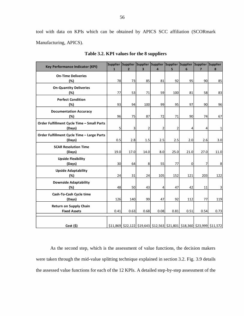
56

tool with data on KPIs which can be obtained by APICS SCC affiliation (SCORmark

Manufacturing, APICS).

Table 3.2. KPI values for the 8 suppliers

As the second step, which is the assessment of value functions, the decision makers

were taken through the mid-value splitting technique explained in section 3.2. Fig. 3.9 details

the assessed value functions for each of the 12 KPIs. A detailed step-by-step assessment of the

Key Performance Indicator (KPI)Supplier

1

Supplier

2

Supplier

3

Supplier

4

Supplier

5

Supplier

6

Supplier

7

Supplier

8

On-Time Deliveries

(%) 78 73 85 81 92 95 90 85

On-Quantity Deliveries

(%) 77 53 71 59 100 81 58 83

Perfect Condition

(%) 93 94 100 99 95 97 90 96

Documentation Accuracy

(%) 96 75 87 72 71 90 74 67

Order Fulfillment Cycle Time – Small Parts

(Days) 5 3 2 2 2 4 4 1

Order Fulfillment Cycle Time – Large Parts

(Days) 0.5 2.8 1.5 2.5 2.5 2.0 2.6 3.0

SCAR Resolution Time

(Days) 19.0 17.0 14.0 8.0 25.0 21.0 27.0 11.0

Upside Flexibility

(Days) 30 64 8 55 77 0 7 8

Upside Adaptability

(%) 24 31 24 105 152 121 203 122

Downside Adaptability

(%) 48 50 43 4 47 42 11 3

Cash-To-Cash Cycle time

(Days) 126 140 99 47 92 112 77 119

Return on Supply Chain

Fixed Assets 0.41 0.63 0.68 0.08 0.81 0.51 0.54 0.73

Cost ($) $11,869 $22,122 $19,643 $12,563 $21,801 $18,360 $23,999 $11,572

57

value function evaluation method using the excel tool is presented in Appendix A for interested

readers.

Figure 3.9: Value functions for the 12 supplier KPIs

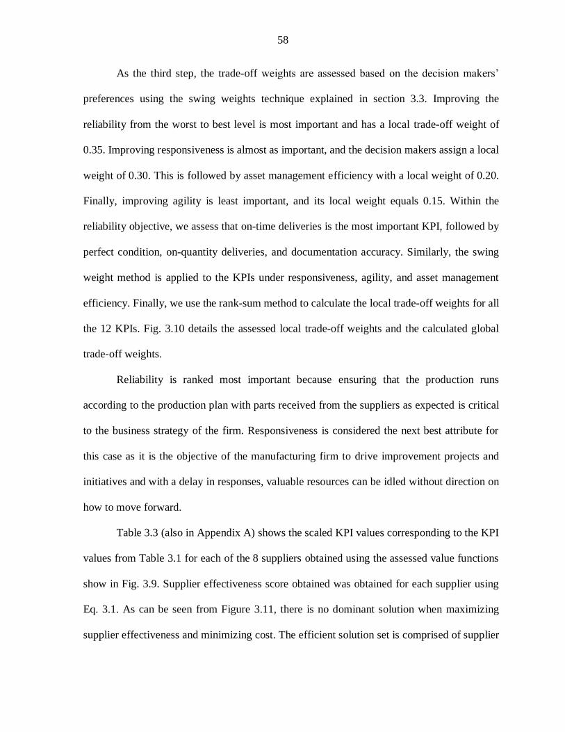
58

As the third step, the trade-off weights are assessed based on the decision makers’

preferences using the swing weights technique explained in section 3.3. Improving the

reliability from the worst to best level is most important and has a local trade-off weight of

0.35. Improving responsiveness is almost as important, and the decision makers assign a local

weight of 0.30. This is followed by asset management efficiency with a local weight of 0.20.

Finally, improving agility is least important, and its local weight equals 0.15. Within the

reliability objective, we assess that on-time deliveries is the most important KPI, followed by

perfect condition, on-quantity deliveries, and documentation accuracy. Similarly, the swing

weight method is applied to the KPIs under responsiveness, agility, and asset management

efficiency. Finally, we use the rank-sum method to calculate the local trade-off weights for all

the 12 KPIs. Fig. 3.10 details the assessed local trade-off weights and the calculated global

trade-off weights.

Reliability is ranked most important because ensuring that the production runs

according to the production plan with parts received from the suppliers as expected is critical

to the business strategy of the firm. Responsiveness is considered the next best attribute for

this case as it is the objective of the manufacturing firm to drive improvement projects and

initiatives and with a delay in responses, valuable resources can be idled without direction on

how to move forward.

Table 3.3 (also in Appendix A) shows the scaled KPI values corresponding to the KPI

values from Table 3.1 for each of the 8 suppliers obtained using the assessed value functions

show in Fig. 3.9. Supplier effectiveness score obtained was obtained for each supplier using

Eq. 3.1. As can be seen from Figure 3.11, there is no dominant solution when maximizing

supplier effectiveness and minimizing cost. The efficient solution set is comprised of supplier

59

8 and supplier 6 since neither of them are dominated by any of the others. Deciding among

these two suppliers require further examination of the decision maker’s preferences concerning

supplier effectiveness and costs (Wall & MacKenzie, 2013).

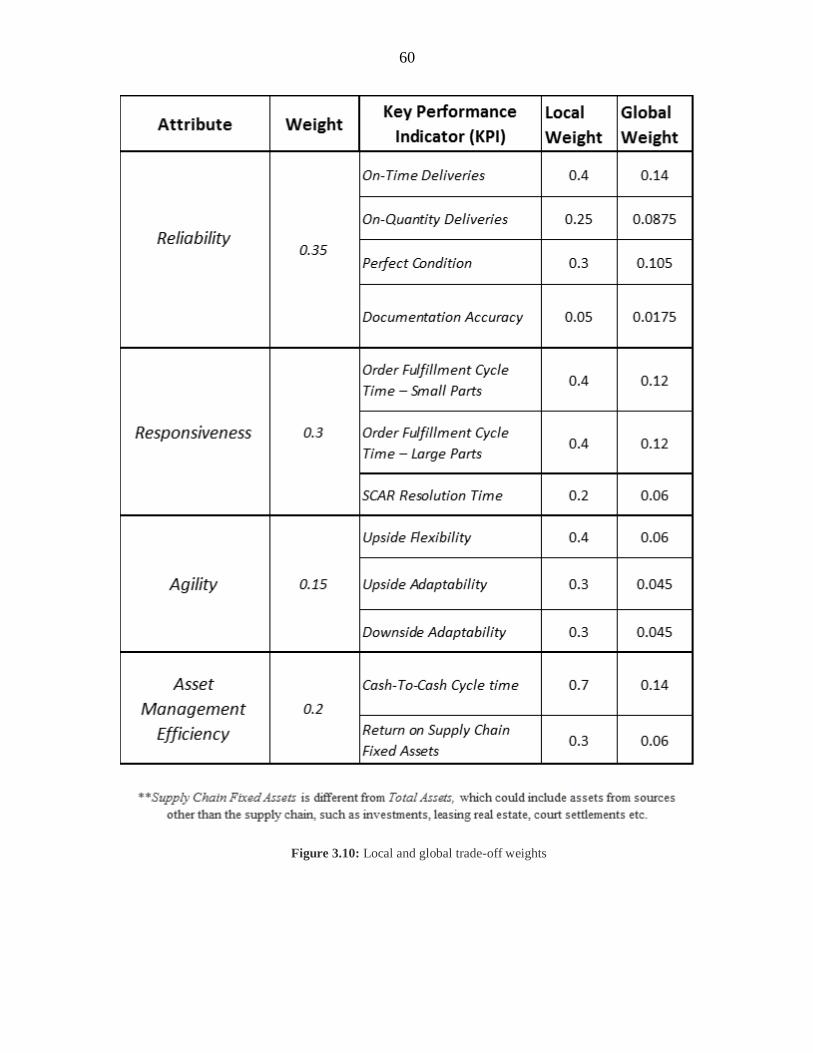
60

Figure 3.10: Local and global trade-off weights

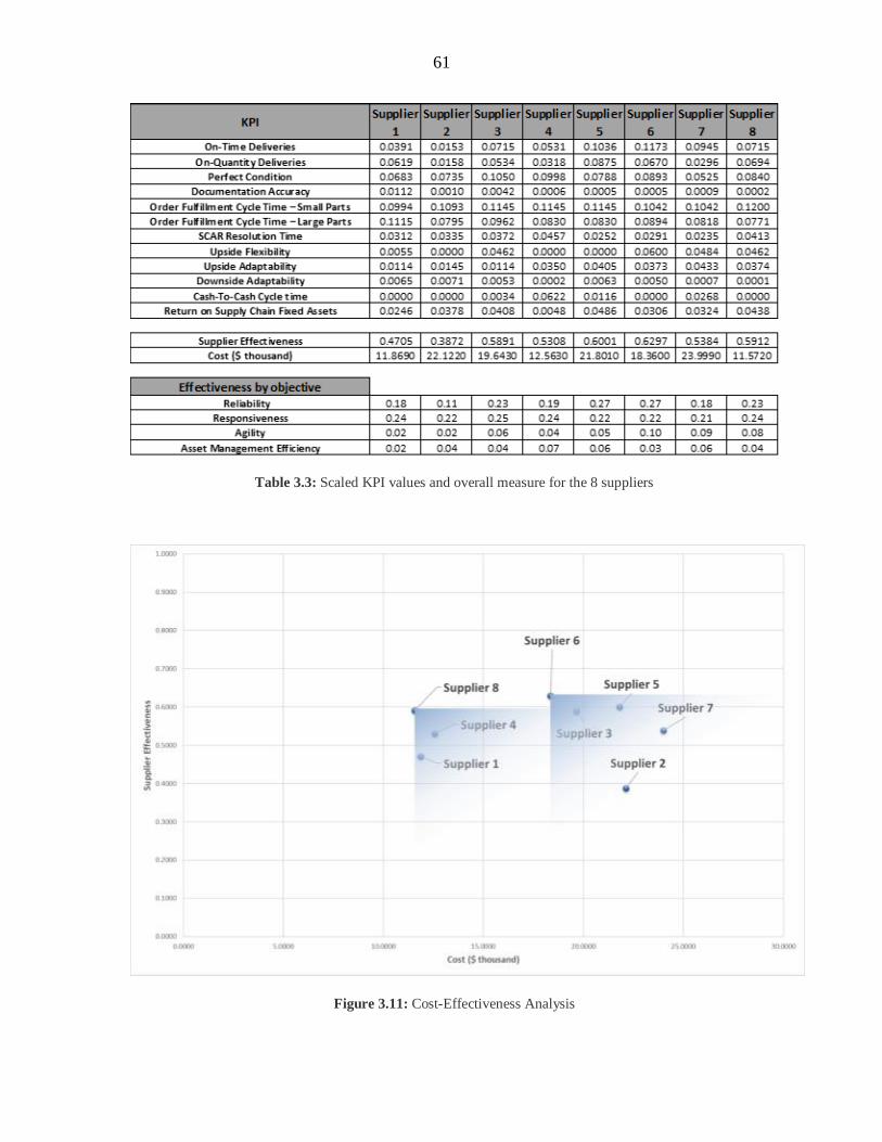
61

Table 3.3: Scaled KPI values and overall measure for the 8 suppliers

Figure 3.11: Cost-Effectiveness Analysis

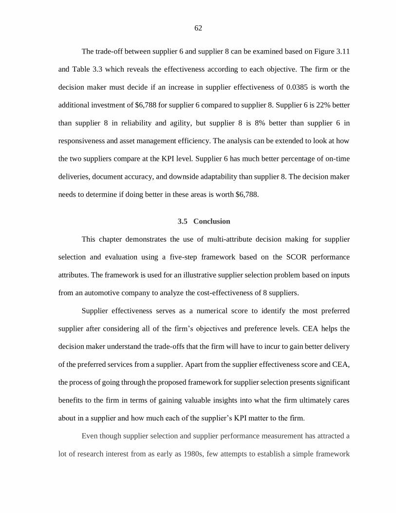
62

The trade-off between supplier 6 and supplier 8 can be examined based on Figure 3.11

and Table 3.3 which reveals the effectiveness according to each objective. The firm or the

decision maker must decide if an increase in supplier effectiveness of 0.0385 is worth the

additional investment of $6,788 for supplier 6 compared to supplier 8. Supplier 6 is 22% better

than supplier 8 in reliability and agility, but supplier 8 is 8% better than supplier 6 in

responsiveness and asset management efficiency. The analysis can be extended to look at how

the two suppliers compare at the KPI level. Supplier 6 has much better percentage of on-time

deliveries, document accuracy, and downside adaptability than supplier 8. The decision maker

needs to determine if doing better in these areas is worth $6,788.

3.5 Conclusion

This chapter demonstrates the use of multi-attribute decision making for supplier

selection and evaluation using a five-step framework based on the SCOR performance

attributes. The framework is used for an illustrative supplier selection problem based on inputs

from an automotive company to analyze the cost-effectiveness of 8 suppliers.

Supplier effectiveness serves as a numerical score to identify the most preferred

supplier after considering all of the firm’s objectives and preference levels. CEA helps the

decision maker understand the trade-offs that the firm will have to incur to gain better delivery

of the preferred services from a supplier. Apart from the supplier effectiveness score and CEA,

the process of going through the proposed framework for supplier selection presents significant

benefits to the firm in terms of gaining valuable insights into what the firm ultimately cares

about in a supplier and how much each of the supplier’s KPI matter to the firm.

Even though supplier selection and supplier performance measurement has attracted a

lot of research interest from as early as 1980s, few attempts to establish a simple framework

63

for supplier selection that incorporates multi-attribute decision-making techniques. In this

chapter, such a framework is presented. This chapter also identifies SCOR as the most

comprehensive and efficient model for supply chain performance measurement from which

supplier performance measurement metrics are derived to evaluate and compare suppliers from

a firm’s perspective. With an illustrative example of the framework’s application, value

functions and trade-off weights that change based upon a firm’s requirements and preferences

are derived. Our analysis demonstrates that the cost-effectiveness of a supplier depends on the

decision maker’s preferences, and the firm should continue to update or reevaluate its

requirements, preferences, and trade-off weights.

64

Acknowledgements

We would like to thank Mike Sherwin and two anonymous personnel from an

automotive company for their advice and feedback during this research and for sharing their

expertise in supplier selection and evaluation.

References

Agarwal, P., Sahai, M., Mishra, V., Bag, M., & Singh, V. (2011). A review of multi-criteria

decision making techniques for supplier evaluation and selection. International

journal of industrial engineering computations, 2(4), 801-810.

Basnet, C., Leung, J. M. Y., & University of Waikato. (2002). Inventory lot sizing with

supplier selection. Hamilton, N.Z: Dept. of Management Systems, University of

Waikato.

Braglia, M., & Petroni, A. (2000). A quality assurance-oriented methodology for handling

trade-offs in supplier selection. International Journal of Physical Distribution &

Logistics Management, 30(2), 96-112.

Bouchereau, V., & Rowlands, H. (2000). Methods and techniques to help quality function

deployment (QFD). Benchmarking: An International Journal, 7(1), 8-20.

Council, S. C. (2012). Supply chain operations reference model: Revision 11.0. Chicago, IL.

Ho, W., Xu, X., & Dey, P. K. (2010). Multi-criteria decision making approaches for supplier

evaluation and selection: A literature review. European Journal of operational

research, 202(1), 16-24.

Huang, S. H., & Keskar, H. (2007). Comprehensive and configurable metrics for supplier

selection. International journal of production economics, 105(2), 510-523.

65

Huan, S. H., Sheoran, S. K., & Wang, G. (2004). A review and analysis of supply chain

operations reference (SCOR) model. Supply Chain Management: An International

Journal, 9(1), 23-29.

Jafari Songhori, M., Tavana, M., Azadeh, A., & Khakbaz, M. H. (2011). A supplier selection

and order allocation model with multiple transportation alternatives. The International

Journal of Advanced Manufacturing Technology, 52(1), 365-376.

Keeney, R. L., & Raiffa, H. (1993). Decisions with multiple objectives: preferences and

value trade-offs. Cambridge university press.

Kocaoğlu, B., Gülsün, B., & Tanyaş, M. (2013). A SCOR based approach for measuring a

benchmarkable supply chain performance. Journal of Intelligent Manufacturing, 1-20.

Li, L. (2007). Incorporating uncertainty into a multicriteria supplier selection problem.

Lima-Junior, F. R., & Carpinetti, L. C. R. (2016). Combining SCOR model and fuzzy

TOPSIS for supplier evaluation and management. International Journal of Production

Economics, 174, 128-141.

Mohammady Garfamy, R., & Martínez Parra, J. L. (2006). Supplier selection and business

process improvement. Universitat Autònoma de Barcelona,.

Moore, R. (2004). Making common sense common practice: Models for manufacturing

excellence. Amsterdam: Elsevier/Butterworth-Heinemann.

Mukherjee, K. (2017). Supplier selection: An MCDA-based approach.

Ravindran, A. R., & Warsing, J. D. P. (2013). Supply Chain Engineering: Models and

Applications. Hoboken: CRC Press.

66

SCORmark Manufacturing. APICS. Retrieved from https://www.apics.org/apics-for-

business/products-and-services/benchmarking/scormark-manufacturing. Date of

access: 2017, Mar 29.

Wall, K. D., & MacKenzie, C. A. (2015). Multiple objective decision making. Military Cost–

Benefit Analysis: Theory and Practice, 197.

Weber, C. A. (1996). A data envelopment analysis approach to measuring vendor

performance. Supply Chain Management: An International Journal, 1(1), 28-39.

Williams, R. A., & Thompson, K. M. (2004). Integrated analysis: Combining risk and

economic assessments while preserving the separation of powers. Risk Analysis,

24(6), 1613-1623.

67

CHAPTER 4. GENERAL CONCLUSIONS

General Discussion

Supply chains have developed over time to meet the demand of delivering products and

services faster and cheaper than before. However, these advances have come at the cost of

expanded defenselessness of supply chains. Since the current global supply chains are highly

connected, the negative impact of disturbances occurring due to new unknown variables can

spread rapidly. To cope with this increased vulnerability, we argued in Chapter 2 that

companies must actively work to manage the risk from its downstream supply chain by

forecasting the impact of a temporary production shut down due to a disruption event. Further,

with today’s increased dependence on supply chain networks, firms are directly exposed to

their suppliers’ risk profiles. This, on the other hand, needs a systematic framework using

effective supplier performance metrics and multi-objective decision making techniques to

select most effective supplier and we demonstrated such a model in Chapter 3.

The focus of this thesis was to develop quantitative methods to analyze supply chain

risk from a firm’s perspective. First, we modeled the different types of customer behaviors as

a probabilistic model to forecast the lost revenue from a production shut-down due to a supply

chain disruption. Second, we presented a new framework for supplier selection and evaluation

using the combination of multi-criteria decision making techniques and the SCOR model.

In the market response model presented in Chapter 2, lost revenue serves as a measure

of risk and enables a firm to foresee the consequences of a production shut down. While the

values of the uncertain parameters p, the probability with which each customer comes back to

the firm, and q, conditional probability that the customer who comes back immediately will

require backorders, are uncertain and beyond the scope of this thesis, we can use the model to

68

derive important risk management insights that would lead to making better decisions

increasing the supply chain resilience of a firm.

Using the framework presented in Chapter 3, decision makers from a firm can

incorporate their own preference within the presented framework to determine the most

preferred supplier and assess the cost effectiveness to select a supplier in different scenarios.

Depending on specific cases such as whether the firm is in a position where it can make trade-

offs on costs and demand higher supplier effectiveness or the firm has a maximum threshold

on costs within which it requires most effective supplier, the COE can be used to select most

cost-efficient supplier.

Recommendations for Future Research

The proposed market response model could be developed further by relaxing some of

the assumptions. For instance, customers may return with different probabilities or

probabilities that change over time. Further extensions to this research can include the

development of a decision-making framework to utilize the mathematical model to determine

the most effective risk management decisions during a supply chain disruption. Another

extension is to model the probability of a supply chain disruption along with the total expected

lost revenue to make sound management decisions regarding investments in preparedness

measures. An optimization model that minimizes the lost revenue during the disruption periods

can also serve as a future extension to this chapter.

Further studies on supplier selection can apply the proposed framework for supplier

selection and evaluation in manufacturing supply chains with different strategies such as lean,

agile, lean etc. Suggestions for future research include further development of objectives

69

hierarchy to include other supplier KPIs that are not covered in the SCOR model. For instance,

a firm may care about expedition capability of a supplier.

The major limitation of the proposed supplier selection framework is the certainty

assumption of supplier KPIs. Hence, in case applications with deterministic metrics, sensitivity

analysis must be carried out to assess the sensitivity of the results to the weights and

preferences. Moreover, the proposed method can be developed further by considering non-

deterministic case of supplier performance where each KPI can be represented by a probability

distribution. Such models that accounts for the uncertainty with supplier performance can use

Bayesian updating for updating supplier performance beyond the supplier selection process. A

firm could update its belief about a supplier and reassess the supplier effectiveness using data

from ERP systems as it continues to work with the supplier and observe the supplier’s

performance. Finally, the Excel tool for supporting supplier selection and evaluation can be

further developed with feedback from practitioners through multiple case studies.

70

APPENDIX A. USING THE EXCEL TOOL

This section describes how decision maker can use the authors’ Excel worksheets, otherwise

known as Excel Tool, to fashion their own multi-objective, cost- effective analysis for supplier

selection. The decision support tool is coded in Microsoft Excel and is customizable. It serves

as a guide for the interaction between an analyst and the decision maker to assess a value

functions and trade-off weights to measure suppliers' effectiveness. This appendix provides

some detail into using the Excel tool to evaluate the cost-effectiveness of a supplier. A

screenshot of excel tool with all the worksheets can be seen in Figure A.1.

Figure A.1: Excel tool interface

The first worksheet named Instructions provide general guidelines for using the tool described

in detail here. The second worksheet named, Supplier KPIs data, lists raw data used for the

supplier selection. The current data is based on the illustrative example presented in the paper.

71

As mentioned in section 3.4, the firm entering a supplier relationship must obtain these KPI

data along with the cost quotations when the suppliers put together their bids. This sheet should

not be modified unless the user has different data or would like to insert another supplier.

Figure A.2: Excel tool interface for assessing value function

The third worksheet named, Mid-value Splitting (template) is the general template that

is used to create value functions for each of the KPIs selected by the decision maker. This

worksheet is duplicated and fashioned for each of the KPI in the objectives hierarchy according

to the decision maker’s preferences using mid-value splitting technique. Worksheets 1 to 12

represent value functions corresponding to the 12 KPIs identified for the supplier selection

problem in the illustrative example (Section 3.4). The first steps to approximating a value

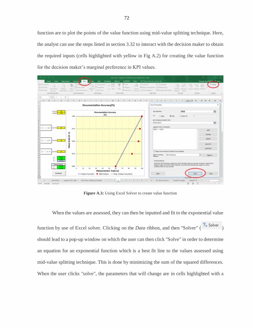
72

function are to plot the points of the value function using mid-value splitting technique. Here,

the analyst can use the steps listed in section 3.32 to interact with the decision maker to obtain

the required inputs (cells highlighted with yellow in Fig A.2) for creating the value function

for the decision maker’s marginal preference in KPI values.

Figure A.3: Using Excel Solver to create value function

When the values are assessed, they can then be inputted and fit to the exponential value

function by use of Excel solver. Clicking on the Data ribbon, and then "Solver" ( )

should lead to a pop-up window on which the user can then click "Solve" in order to determine

an equation for an exponential function which is a best fit line to the values assessed using

mid-value splitting technique. This is done by minimizing the sum of the squared differences.

When the user clicks "solve", the parameters that will change are in cells highlighted with a

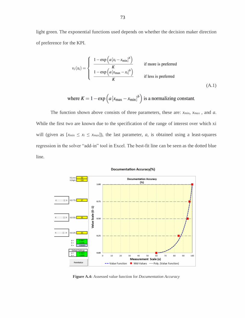
73

light green. The exponential functions used depends on whether the decision maker direction

of preference for the KPI.

(A.1)

The function shown above consists of three parameters, these are: xmin, xmax , and a.

While the first two are known due to the specification of the range of interest over which xi

will (given as [xmin ≤ xi ≤ xmax]), the last parameter, a, is obtained using a least-squares

regression in the solver “add-in” tool in Excel. The best-fit line can be seen as the dotted blue

line.

Figure A.4: Assessed value function for Documentation Accuracy

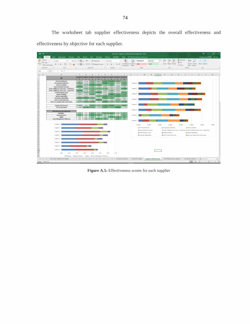
74

The worksheet tab supplier effectiveness depicts the overall effectiveness and

effectiveness by objective for each supplier.

Figure A.5: Effectiveness scores for each supplier

Quantitative models for supply chain risk analysis from a ...Quantitative models for supply chain...

Documents

Transcript of Quantitative models for supply chain risk analysis from a ...Quantitative models for supply chain...