Quantitative Finance - Fixed Income securities -...

Stochastic Interest Rates The bond pricing equation Solution of a bond pricing equation Named Models

Quantitative Finance - FixedIncome securities

Lecture 3

October 27, 2014


Outline

1 Stochastic Interest Rates

2 The bond pricing equation

3 Solution of a bond pricing equation

4 Named ModelsVasicek ModelCox, Ingersoll and Ross


Introduction

So far we considered that the interest ratesare either constant or a known function oftime

From now on, we will be modeling interestrates using a single source of randomness -one-factor interest rate modeling

The model leads to a parabolic partialdifferential equation for the prices of bondsand other interest rate derivative products.


Stochastic Interest Rates

Since we cannot realistically forecast thefuture course of an interest rate, it is naturalto model it as a random variable

We start by modeling the behavior of r, theinterest rate received by the shortestpossible deposit also called the spotinterest rate

Suppose that the interest rate r is governedby a stochastic differential equation

dr = µ(r , t)dt + σ(r , t)dW


where µ(r , t) and σ(r , t) determine thebehaviour of r .

We use this random walk to derive a partialdifferential equation for the price of a bond usingsimilar arguments to those in the derivation ofthe Black-Scholes equation


The bond pricing equation

Since the interest rates are stochastic, wedenote the price of a bond by V (r , t ; T )

Pricing a bond: Is there an underlying assetwith which to hedge?

We are not modeling a traded asset; thetraded asset (the bond, say) is a derivativeof our independent variable r


The only way to construct a hedgedportfolio is by hedging one bond with abond of a different maturity

Set up a portfolio containing two bonds withdifferent maturities T1 and T2 with priceV1(r , t ; T1) and V2(r , t ; T2), respectively

We hold one of the former and a number−4 of the latter. We have

Π = V1 −4V2


The change in the portfolio in a time dt isgiven by

dΠ = ∂V1∂t dt + ∂V1

∂r dr + 12σ

2 ∂2V1∂r2 dt −

4(∂V2∂t dt + ∂V2

∂r dr + 12σ

2 ∂2V2∂r2 dt

)Which of these terms are random?

Eliminate the randomness in dΠ

The portfolio is then riskless dΠ = rΠdt

Collecting all V1 terms on the left-hand sideand all V2 terms on the right-hand side wefind that


∂V1∂t + 1

2σ2 ∂2V1

∂r2 − rV1∂V1∂r

=∂V2∂t + 1

2σ2 ∂2V2

∂r2 − rV2∂V2∂r

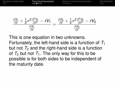
This is one equation in two unknowns.Fortunately, the left-hand side is a function of T1but not T2 and the right-hand side is a functionof T2 but not T1. The only way for this to bepossible is for both sides to be independent ofthe maturity date.


Dropping the subscript∂V∂t + 1

2σ2 ∂2V∂r2 − rV

∂V∂r

= a (r , t)

for some function a(r , t)

It is always possible to writea(r , t) = σ(r , t)λ(r , t)− µ(r , t)

The bond equation then becomes

∂V∂t

+12σ2∂

2V∂r2 − rV + (σ(r , t)λ(r , t)− µ(r , t))

∂V∂r

= 0 (1)


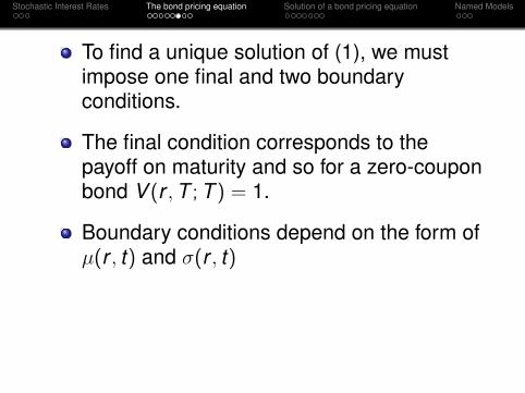
To find a unique solution of (1), we mustimpose one final and two boundaryconditions.

The final condition corresponds to thepayoff on maturity and so for a zero-couponbond V (r ,T ; T ) = 1.

Boundary conditions depend on the form ofµ(r , t) and σ(r , t)


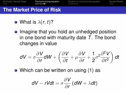
The Market Price of Risk

What is λ(r , t)?

Imagine that you hold an unhedged positionin one bond with maturity date T . The bondchanges in value

dV = σ∂V∂r

dW +

(∂V∂t

+ µ∂V∂r

+12σ2∂

2V∂r2

)dt

Which can be written on using (1) as

dV − rVdt = σ∂V∂r

(dW + λdt)


The right-hand side of this expressioncontains two terms: a deterministic term ind t and a random term in dW

Not a riskless portfolio

The deterministic term may be interpretedas the excess return above the risk-free ratefor accepting a certain level of risk. In returnfor taking the extra risk the portfolio profitsby an extra λdt per unit of extra risk dW


Solution of a bond pricing equation

We have built up the bond pricing equationfor an arbitrary model that is we have notspecified µ− λσ and σ

How can we choose these functions to giveus a good model?

Is simple lognormal random walk suitablefor r?


Since a simple lognormal random walk wouldpredict exponentially rising or falling interestrates, this rules out the equity price model as aninterest rate model


Let us examine some choices for therisk-neutral drift and volatility that lead totractable modelsLet

µ(r , t)− λ(r , t)σ(r , t) = η(t)− γ(t)r

σ(r , t) =√α(t)r + β(t)

(2)

By suitably restricting these time-dependentfunctions, we can ensure that the randomwalk for r has the following nice properties:


Positive interest rates: Interest rates arepositive. With the above model the spot ratecan be bounded below by a positivenumber if α(t) > 0 and β ≤ 0. The lowerbound is −β/α.

Mean reversion: Examining the drift term,we see that for large r the (risk-neutral)interest rate will tend to decrease towardsthe mean. We also want the lower bound tobe non-attainable. This can be attained byη(t) ≥ −β(t)γ(t)/α(t) + α(t)/2 (Exercise)


Solution of the bond pricing equation

With the choices of µ(r , t) and σ(r , t), thesolution of bond pricing equation for a zerocoupon bond is of the form

Z (r , t ; T ) = expA(t ;T )−B(t ;T )r

Substitute the expression for Z in the bondpricing equation (1), we get


∂A∂t− r

∂B∂t

+12σ2B2 − (µ− λσ)B − r = 0 (3)

Differentiating with respect to r gives

−∂B∂t

+12

B2 ∂

∂rσ2 − B

∂

∂r(µ− λσ)− 1 = 0

Differentiate again w.r.t.r and equate thepowers of T on both sides to get (2)


The substitution of (2) for interest rates in 3for bond pricing equation for ZCB, yields thefollowing equations for A and B

∂A∂t

= η(t)B − 12β(t)B2

∂B∂t

=12α(t)B2 + γ(t)B − 1

In order to satisfy the final data thatZ (r ,T ; T ) = 1 we must have A(T ; T ) = 0and B(T ; T ) = 0We will solve this for constant parameters innext lecture.


Vasicek Model

The Vasicek model takes the form withα = 0, β > 0 and with all other parametersindependent of time

dr = (η − γr)dt +√βdW

This model is so tractable that there areexplicit formulae for many interest ratederivatives

The model is mean reverting to a constantlevel

Interest rates can easily go negative


Cox, Ingersoll and Ross

The CIR model takes the form with β = 0,and again no time dependence in theparameters

dr = (η − γr)dt +√αrdW

The spot rate is mean reverting

Nonnegative interest rates

Interest rates would stay positive if η > α/2.


More generally, when the rate is at a low level(close to zero), the standard deviation alsobecomes very small, which dampens the effectof the random shock on the rate. Consequently,when the rate gets close to zero, its evolutionbecomes dominated by the drift factor, whichpushes the rate upwards

Quantitative Finance - Fixed Income securities -...

Documents

Transcript of Quantitative Finance - Fixed Income securities -...