Takustraße 7D-14195 Berlin-Dahlem

GermanyZuse Institute Berlin

SEBASTIAN GOTSCHEL, CHRISTIANE MAIERHOFER,JAN P. MULLER, NICK ROTHBART, MARTIN WEISER

Quantitative Defect Reconstruction inActive Thermography for Fiber-Reinforced

Composites

ZIB Report 16-13 (March 2016)

Zuse Institute BerlinTakustraße 7D-14195 Berlin-Dahlem

Telefon: 030-84185-0Telefax: 030-84185-125

e-mail: bibliothek@zib.deURL: http://www.zib.de

ZIB-Report (Print) ISSN 1438-0064ZIB-Report (Internet) ISSN 2192-7782

Quantitative Defect Reconstruction in Active

Thermography for Fiber-Reinforced Composites

Sebastian Gotschel∗ Christiane Maierhofer† Jan P. Muller†

Nick Rothbart† Martin Weiser∗

March 23, 2016

Abstract

Carbon-fiber reinforced composites are becoming more and more im-portant in the production of light-weight structures, e.g., in the automotiveand aerospace industry. Thermography is often used for non-destructivetesting of these products, especially to detect delaminations between dif-ferent layers of the composite.

In this presentation, we aim at methods for defect reconstruction fromthermographic measurements of such carbon-fiber reinforced composites.The reconstruction results shall not only allow to locate defects, but alsogive a quantitative characterization of the defect properties. We discussthe simulation of the measurement process using finite element methods,as well as the experimental validation on flat bottom holes.

Especially in pulse thermography, thin boundary layers with steep tem-perature gradients occurring at the heated surface need to be resolved.Here we use the combination of a 1D analytical solution combined withnumerical solution of the remaining defect equation. We use the simula-tions to identify material parameters from the measurements.

Finally, fast heuristics for reconstructing defect geometries are appliedto the acquired data, and compared for their accuracy and utility in de-tecting different defects like back surface defects or delaminations.

Introduction

Active thermography is a fast and contactless method for nondestructive testingof a wide range of structures. It is based on the generation of a non-stationaryheat flux inside the object under investigation, and time-resolved measurementsof its surface temperature by an infrared camera. Defects and inhomogeneityin the material with thermal properties differing from the surrounding materialcan be detected from spatial temperature differences within a particular timerange. Often, quantitative information about such defects, like depth, residualwall thickness or lateral extent need to be extracted from the measurements.

∗Zuse Institute Berlin, Berlin, Germany†BAM Bundesanstalt fur Materialforschung und -prufung, Berlin, Germany

1

Models like PPT (pulse phase thermography) [1] and TSR (thermographic sig-nal reconstruction) [2], considering solely the heat flow normal to the surfaceof the specimen, deliver a fast way to assess the size and to a certain extentthe depth of the defect within the sample. Since they are based on analyticalsolutions of simplified models, they are well suited for practical applications.

For a more detailed inspection in order to obtain quantitative results, isstrongly desirable to take lateral heat flows into account. A viable path toreconstruct the sub-surface defects of the specimen is to numerically solve theunderlying PDE and optimize the geometric data and the thermal materialparameters iteratively. This way to solve the inverse problem is computationallyexpensive, but paves the road to extract much more detailed information fromthe measurements, compared to the analytical reconstruction methods. In thiscontribution, we describe experiments, simulation and reconstruction methodsfor carbon-fiber reinforced composites.

1 Experiments

Two samples (produced by ZfL Haldensleben) have been investigated by flashthermography [3]. One sample consists of pure epoxy resin (the almost isotropicmatrix material of CFRP), the other one of unidirectional CFRP. A photoof each specimen is shown in Figure 1 a) and b). The second specimen wasproduced using the RTM-light process. 34 layers of woven carbon filaments,having a weight of 140g/m2 were aggregated with their fibers in parallel (fiberorientation is in vertical direction in Figure 1 b). The layers are plain warpreinforced. At the surface two layers turned by 90° with respect to the restof the layers are added. Finally, epoxy resin has been added under vacuumconditions inside a form. The sample has been stored for 24h at a temperature of50−60 °C. The layer structure can be clearly seen in Figure 1 c). Both specimenshave defined flat bottom holes of distinct diameter and depth machined on thesample in a similar pattern. The holes serve as defined defects on the back sideof the investigated flat surface and enable to assess the reconstruction process.The sample made of pure epoxy resin has an average thickness of 5.5 mm, theCFRP sample of 5.8 mm. Both samples have a dimension of 200 × 200 mm2.The residual wall thickness of the holes, having diameters between 4 and 24 mm,amounts from 0.5 mm up to 4.2 mm. The surface of the sample made of epoxyresin was blackened using two layers of paint (Tetenal camera paint).

Time-resolved thermography has been carried out using flash excitation ofthe front surface to obtain information on the back side of the specimen. Thisrepresents a model case for non-destructive testing of materials. Four flashlamps (Hensel Studio Technik, EH PRO 6000), having 6 kJ energy each, areheating the plane surface. The flash lamps have a maximum radiation temper-ature of 5000 K, the main infrared (IR) part of the spectrum is mitigated by twoPMMA-plates having a thickness of 8 mm. Thus the specimen is heated mainlyby visible light within a short time. The light intensity of the flash lamps can bedescribed with respect to time by an exponential decay function, the half timeamounts to 2.0 ms. The flash duration has been measured using a photodiode

2

(Thorlabs, PDA36A-EC) with metallic neutral density filters mounted on itsfront. The flash lamps are aligned for a homogeneous illumination of the samplesurface. The main axis of the lamps is aligned in an angle of 15 ° relative to thenormal to the front of the specimen, at a distance of 45 cm typically. The IRcamera is positioned behind the gap between the flash lamps. The epoxy resinas well as the CFRP sample is supported by a frame made of corrugated board,which shields the IR camera from the flash light as well as thermally insolatesthe sample.

The IR camera (Infratec, ImageIR 9830), equipped with a 50 mm lens,records the temperature using a fast InSb-focal plane array in the spectralwavelength range of 3 − 5µm. It has a maximal resolution of 1280 × 1024pixels and the transient temperature of the specimen has been imaged at aframe rate of 10 Hz (full frame) and 180 Hz (half frame). For synchronization ofthe flash lamps with the camera a custom made active box (Infratec) is used.Calibration ranges for the temperatures from 0− 60 °C (integration time of thesensor 640µs) and 20− 100 °C (integration time 260µs) are used.

In addition to the epoxy resin or CFRP plates a blackened piece of silvermounted next to the sample is utilized to estimate the irradiation [4]. Theenergy density deposited on the surface amounts to (0.27± 0.01) J/cm2.

The specimens have been investigated using two configurations: the IR cam-era viewing the illuminated front surface of the sample (reflection configuration)for creating the experimental data to reconstruct the defects, as well as the IRcamera viewing the back surface (transmission configuration). The latter set-upenables to measure the in-depth thermal diffusivity of the materials using themethod of Parker et al. [3].

The images of the camera are saved in a binary file format of the Irbis3software (Infratec). The transient signal, consisting of 2000 frames typically,is loaded into the programming language Matlab, in order to prepare the datafor the numeric reconstruction method. A background image, taken before theflash heated the sample, is subtracted from the transient temperature signal.Only the frames recorded after the flash are used for the comparison to thesimulation.

To determine the thermal lateral diffusivity on the surface of the epoxy resinand CFRP a distinct method is used. A laser (laserline LDM 500-20) is coupledinto an optics generating a line focus. The beam waist has a Gaussian profilein x-direction (FWHM of 1 mm) and a homogeneous intensity distribution iny-direction (spreading over 36 mm). The optical axis of the caustics is alignedin an angle of 30 ° with respect to the surface normal of the specimen. The laserruns at a wavelength of 935 nm and illuminates the sample for 100 ms with apower of about 15 W. Due to the absorption of the IR laser light the sampleis heated to temperatures up to 90 °C. A fast IR camera (Infratec, ImageIR8300) measures the thermal signal in the MWIR range from 2 − 5µm with aframerate of 180 Hz. A cooled InSb focal plane array, having 640 × 512 pixelsin combination with a lens (f/2.0, resolution 0.18 mm/pixel) is used to recordthe temporal evolution of the surface temperature, a calibration of 10− 100 °C(485µs integration time) is used. The protraction of the width of the hot areais utilized to obtain the in-plane diffusivity perpendicular to the laser line. The

3

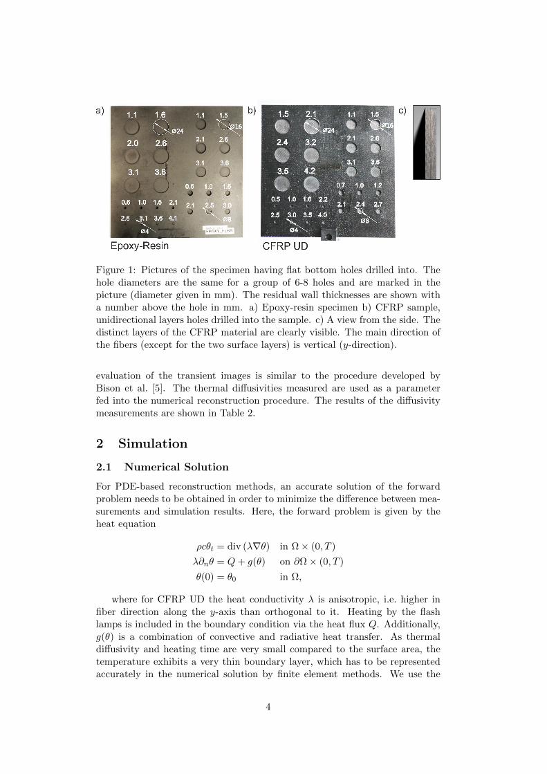
Figure 1: Pictures of the specimen having flat bottom holes drilled into. Thehole diameters are the same for a group of 6-8 holes and are marked in thepicture (diameter given in mm). The residual wall thicknesses are shown witha number above the hole in mm. a) Epoxy-resin specimen b) CFRP sample,unidirectional layers holes drilled into the sample. c) A view from the side. Thedistinct layers of the CFRP material are clearly visible. The main direction ofthe fibers (except for the two surface layers) is vertical (y-direction).

evaluation of the transient images is similar to the procedure developed byBison et al. [5]. The thermal diffusivities measured are used as a parameterfed into the numerical reconstruction procedure. The results of the diffusivitymeasurements are shown in Table 2.

2 Simulation

2.1 Numerical Solution

For PDE-based reconstruction methods, an accurate solution of the forwardproblem needs to be obtained in order to minimize the difference between mea-surements and simulation results. Here, the forward problem is given by theheat equation

ρcθt = div (λ∇θ) in Ω× (0, T )

λ∂nθ = Q+ g(θ) on ∂Ω× (0, T )

θ(0) = θ0 in Ω,

where for CFRP UD the heat conductivity λ is anisotropic, i.e. higher infiber direction along the y-axis than orthogonal to it. Heating by the flashlamps is included in the boundary condition via the heat flux Q. Additionally,g(θ) is a combination of convective and radiative heat transfer. As thermaldiffusivity and heating time are very small compared to the surface area, thetemperature exhibits a very thin boundary layer, which has to be representedaccurately in the numerical solution by finite element methods. We use the

4

hybrid analytic-numerical method developed in [6] to obtain accurate solutionsin reasonable computing times. The implementation is done using the C++finite element toolbox Kaskade7 [7].

2.2 Results

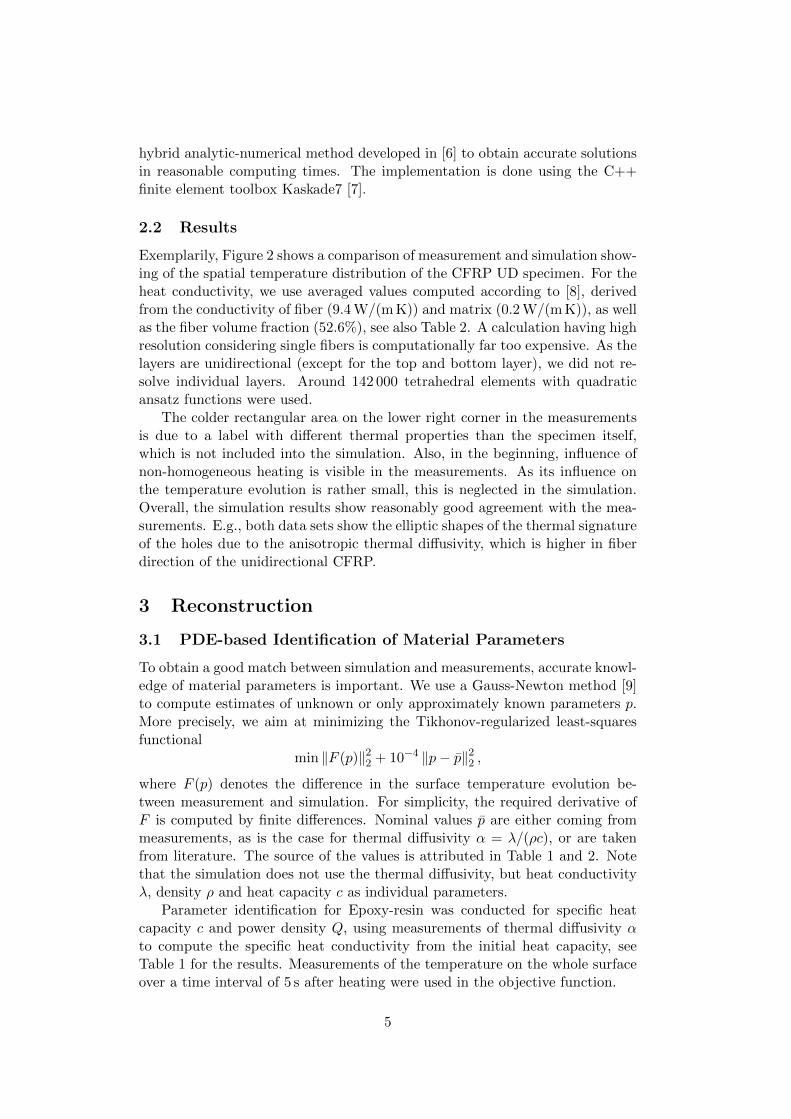
Exemplarily, Figure 2 shows a comparison of measurement and simulation show-ing of the spatial temperature distribution of the CFRP UD specimen. For theheat conductivity, we use averaged values computed according to [8], derivedfrom the conductivity of fiber (9.4 W/(m K)) and matrix (0.2 W/(m K)), as wellas the fiber volume fraction (52.6%), see also Table 2. A calculation having highresolution considering single fibers is computationally far too expensive. As thelayers are unidirectional (except for the top and bottom layer), we did not re-solve individual layers. Around 142 000 tetrahedral elements with quadraticansatz functions were used.

The colder rectangular area on the lower right corner in the measurementsis due to a label with different thermal properties than the specimen itself,which is not included into the simulation. Also, in the beginning, influence ofnon-homogeneous heating is visible in the measurements. As its influence onthe temperature evolution is rather small, this is neglected in the simulation.Overall, the simulation results show reasonably good agreement with the mea-surements. E.g., both data sets show the elliptic shapes of the thermal signatureof the holes due to the anisotropic thermal diffusivity, which is higher in fiberdirection of the unidirectional CFRP.

3 Reconstruction

3.1 PDE-based Identification of Material Parameters

To obtain a good match between simulation and measurements, accurate knowl-edge of material parameters is important. We use a Gauss-Newton method [9]to compute estimates of unknown or only approximately known parameters p.More precisely, we aim at minimizing the Tikhonov-regularized least-squaresfunctional

min ‖F (p)‖22 + 10−4 ‖p− p‖22 ,

where F (p) denotes the difference in the surface temperature evolution be-tween measurement and simulation. For simplicity, the required derivative ofF is computed by finite differences. Nominal values p are either coming frommeasurements, as is the case for thermal diffusivity α = λ/(ρc), or are takenfrom literature. The source of the values is attributed in Table 1 and 2. Notethat the simulation does not use the thermal diffusivity, but heat conductivityλ, density ρ and heat capacity c as individual parameters.

Parameter identification for Epoxy-resin was conducted for specific heatcapacity c and power density Q, using measurements of thermal diffusivity αto compute the specific heat conductivity from the initial heat capacity, seeTable 1 for the results. Measurements of the temperature on the whole surfaceover a time interval of 5 s after heating were used in the objective function.

5

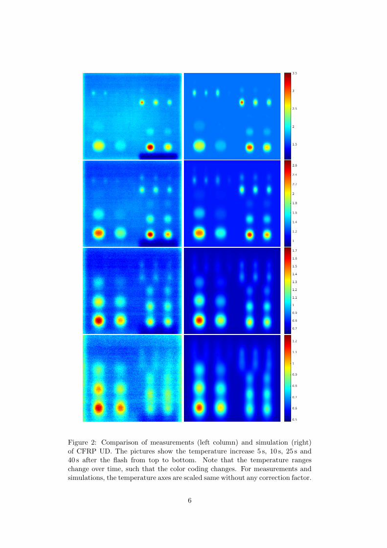
Figure 2: Comparison of measurements (left column) and simulation (right)of CFRP UD. The pictures show the temperature increase 5 s, 10 s, 25 s and40 s after the flash from top to bottom. Note that the temperature rangeschange over time, such that the color coding changes. For measurements andsimulations, the temperature axes are scaled same without any correction factor.

6

Epoxy

Parameter nominal identified

Q [W/m2] 1 040 000± 40 0001 1 007 945

α [m2/s] along z: not identified;(1.3± 0.2) · 10−7 λ = 0.25 W/(m K)

used for all directions used for all directions

c [J/(kg K)] 1700 1674.9

Table 1: Material parameters for Epoxy-resin.1 calculated from the measured energy density of 0.27 J/cm2 and the flashduration of 2.0 ms (half time).

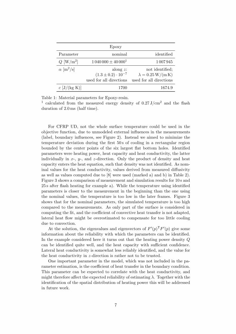
For CFRP UD, not the whole surface temperature could be used in theobjective function, due to unmodeled external influences in the measurements(label, boundary influences, see Figure 2). Instead we aimed to minimize thetemperature deviation during the first 50 s of cooling in a rectangular regionbounded by the center points of the six largest flat bottom holes. Identifiedparameters were heating power, heat capacity and heat conductivity, the latterindividually in x-, y-, and z-direction. Only the product of density and heatcapacity enters the heat equation, such that density was not identified. As nom-inal values for the heat conductivity, values derived from measured diffusivityas well as values computed due to [8] were used (marked a) and b) in Table 2).Figure 3 shows a comparison of measurement and simulation results for 10 s and25 s after flash heating for example a). While the temperature using identifiedparameters is closer to the measurement in the beginning than the one usingthe nominal values, the temperature is too low in the later frames. Figure 3shows that for the nominal parameters, the simulated temperature is too highcompared to the measurements. As only part of the surface is considered incomputing the fit, and the coefficient of convective heat transfer is not adapted,lateral heat flow might be overestimated to compensate for too little coolingdue to convection.

At the solution, the eigenvalues and eigenvectors of F ′(p)TF ′(p) give someinformation about the reliability with which the parameters can be identified.In the example considered here it turns out that the heating power density Qcan be identified quite well, and the heat capacity with sufficient confidence.Lateral heat conductivity is somewhat less reliably identified, and the value forthe heat conductivity in z-direction is rather not to be trusted.

One important parameter in the model, which was not included in the pa-rameter estimation, is the coefficient of heat transfer in the boundary condition.This parameter can be expected to correlate with the heat conductivity, andmight therefore affect the expected reliability of estimating λ. Together with theidentification of the spatial distribution of heating power this will be addressedin future work.

7

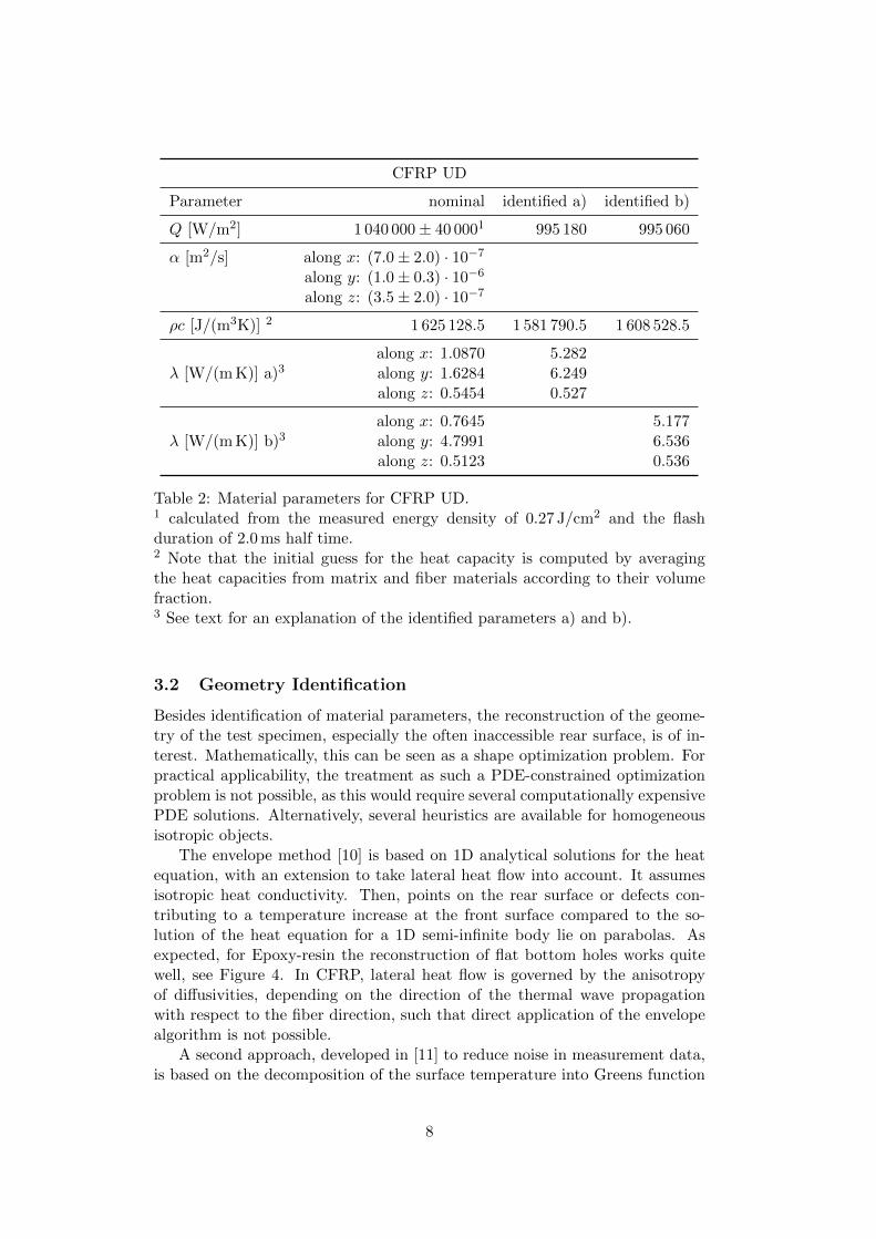
CFRP UD

Parameter nominal identified a) identified b)

Q [W/m2] 1 040 000± 40 0001 995 180 995 060

α [m2/s] along x: (7.0± 2.0) · 10−7

along y: (1.0± 0.3) · 10−6

along z: (3.5± 2.0) · 10−7

ρc [J/(m3K)] 2 1 625 128.5 1 581 790.5 1 608 528.5

along x: 1.0870 5.282λ [W/(m K)] a)3 along y: 1.6284 6.249

along z: 0.5454 0.527

along x: 0.7645 5.177λ [W/(m K)] b)3 along y: 4.7991 6.536

along z: 0.5123 0.536

Table 2: Material parameters for CFRP UD.1 calculated from the measured energy density of 0.27 J/cm2 and the flashduration of 2.0 ms half time.2 Note that the initial guess for the heat capacity is computed by averagingthe heat capacities from matrix and fiber materials according to their volumefraction.3 See text for an explanation of the identified parameters a) and b).

3.2 Geometry Identification

Besides identification of material parameters, the reconstruction of the geome-try of the test specimen, especially the often inaccessible rear surface, is of in-terest. Mathematically, this can be seen as a shape optimization problem. Forpractical applicability, the treatment as such a PDE-constrained optimizationproblem is not possible, as this would require several computationally expensivePDE solutions. Alternatively, several heuristics are available for homogeneousisotropic objects.

The envelope method [10] is based on 1D analytical solutions for the heatequation, with an extension to take lateral heat flow into account. It assumesisotropic heat conductivity. Then, points on the rear surface or defects con-tributing to a temperature increase at the front surface compared to the so-lution of the heat equation for a 1D semi-infinite body lie on parabolas. Asexpected, for Epoxy-resin the reconstruction of flat bottom holes works quitewell, see Figure 4. In CFRP, lateral heat flow is governed by the anisotropyof diffusivities, depending on the direction of the thermal wave propagationwith respect to the fiber direction, such that direct application of the envelopealgorithm is not possible.

A second approach, developed in [11] to reduce noise in measurement data,is based on the decomposition of the surface temperature into Greens function

8

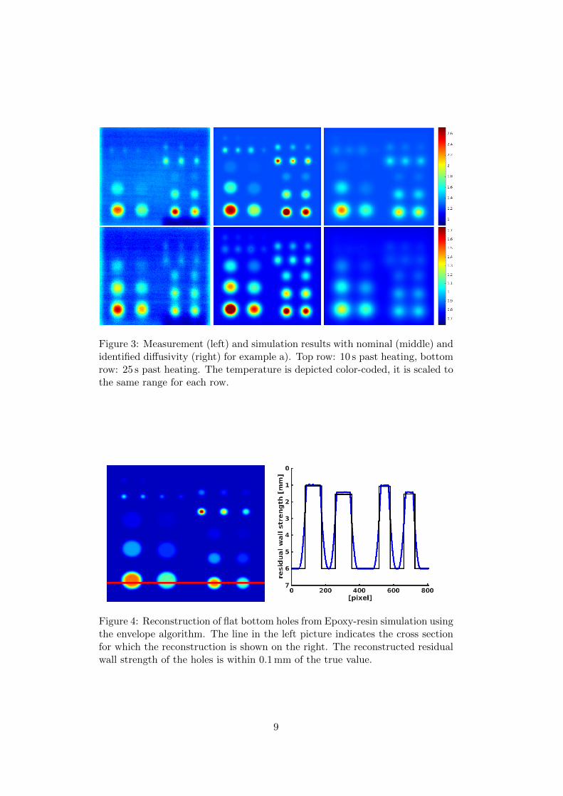
Figure 3: Measurement (left) and simulation results with nominal (middle) andidentified diffusivity (right) for example a). Top row: 10 s past heating, bottomrow: 25 s past heating. The temperature is depicted color-coded, it is scaled tothe same range for each row.

Figure 4: Reconstruction of flat bottom holes from Epoxy-resin simulation usingthe envelope algorithm. The line in the left picture indicates the cross sectionfor which the reconstruction is shown on the right. The reconstructed residualwall strength of the holes is within 0.1 mm of the true value.

9

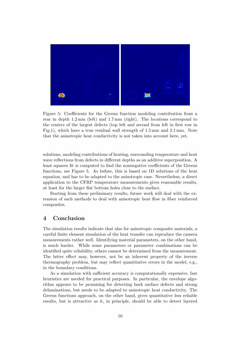
Figure 5: Coefficients for the Greens function modeling contribution from arear in depth 1.2 mm (left) and 1.7 mm (right). The locations correspond tothe centers of the largest defects (top left and second from left in first row inFig.1), which have a true residual wall strength of 1.5 mm and 2.1 mm. Notethat the anisotropic heat conductivity is not taken into account here, yet.

solutions, modeling contributions of heating, surrounding temperature and heatwave reflections from defects in different depths as an additive superposition. Aleast squares fit is computed to find the nonnegative coefficients of the Greensfunctions, see Figure 5. As before, this is based on 1D solutions of the heatequation, and has to be adapted to the anisotropic case. Nevertheless, a directapplication to the CFRP temperature measurements gives reasonable results,at least for the larger flat bottom holes close to the surface.

Starting from these preliminary results, future work will deal with the ex-tension of such methods to deal with anisotropic heat flow in fiber reinforcedcomposites.

4 Conclusion

The simulation results indicate that also for anisotropic composite materials, acareful finite element simulation of the heat transfer can reproduce the camerameasurements rather well. Identifying material parameters, on the other hand,is much harder. While some parameters or parameter combinations can beidentified quite reliability, others cannot be determined from the measurement.The latter effect may, however, not be an inherent property of the inversethermography problem, but may reflect quantitative errors in the model, e.g.,in the boundary conditions.

As a simulation with sufficient accuracy is computationally expensive, fastheuristics are needed for practical purposes. In particular, the envelope algo-rithm appears to be promising for detecting back surface defects and strongdelaminations, but needs to be adapted to anisotropic heat conductivity. TheGreens functions approach, on the other hand, gives quantitative less reliableresults, but is attractive as it, in principle, should be able to detect layered

10

delaminations, e.g., impact damages.

References

[1] X. Maldague and S. Marinetti, Journal of Applied Physics 79, 2694 (1996)

[2] S. M. Shepard, Proceedings of SPIE 4360, 511 (2001)

[3] W. J. Parker, R. J. Jenkins, C. P. Butler, and G. L. Abbott, Journal ofApplied Physics 32, 1679 (1961), doi: 10.1063/1.1728417

[4] R. Krankenhagen and C. Maierhofer, Infrared Physics & Technology 67,363 (2014), doi: 10.1016/j.infrared.2014.07.012

[5] P. Bison, F. Cernuschi, and S. Capelli, Surface and Coatings Technology205, 3128 (2011), doi: 10.1016/j.surfcoat.2010.11.013

[6] M. Weiser, M. Rollig, R. Arndt, and B. Erdmann, Heat Mass Transfer 47,1419 (2010)

[7] S. Gotschel, M. Weiser, and A. Schiela, Advances in DUNE, 101 (2012)

[8] F. Lopez, V. de Paulo Nicolau, C. Ibarra-Castanedo, and X. Maldague,International Journal of Thermal Sciences 86, 325 (2014)

[9] P. Deuflhard. Newton Methods for Nonlinear Problems. Affine Invarianceand Adaptive Algorithms. Springer (2006)

[10] S. Gotschel, M. Weiser, C. Maierhofer, R. Richter, and M. Rollig. in: O.Buyukozturk et al. (Eds.) Nondestructive Testing of Materials and Struc-tures, RILEM Bookseries, Vol. 6, 83 (2013)

[11] S. Gotschel, M. Weiser, Ch. Maierhofer, R. Richter. QIRT-2012-167, Pro-ceedings of the 11th QIRT conference (2012)

11