Quantitative Business Analysis (QBA)
195
Quantitative Business Analysis (QBA) I. Lindner and J.R. van den Brink
Transcript of Quantitative Business Analysis (QBA)

Quantitative Business Analysis (QBA)
I. Lindner and J.R. van den Brink

Q tit ti B i A l iQuantitative Business AnalysisDates lectures:Dates lectures:October 31, November 7, 14, 21, 28,
December 5December 5
Ti 11 00 12 45Time: 11:00-12:45, Location: WN-KC 137
Quantitative Methods (QBA) 2

Q tit ti B i A l iQuantitative Business Analysis• T torials: T esda s and Wednesda s• Tutorials: Tuesdays and Wednesdays• Prepare exercises beforehand! • Program for the first two weeks:
Exercises from chapter “Topic E1 –Exercises Decision Analysis”: week 1: 1.1, 1.2, 1.3, 1.5, 1.8week 2: 1.4, 1.6, 1.7, 1.9
Quantitative Methods (QBA) 3

Quantitative Business AnalysisQuantitative Business AnalysisContents of the Course
Week 1-2 (Ines Lindner)1 Decision Analysis using Decision Trees1. Decision Analysis using Decision Trees
W k 3 6 (R é d B i k)Week 3-6 (René van den Brink)2. Strategic Thinking - Noncooperative Games
Quantitative Methods (QBA) 4

Quantitative Business Analysis
• Book “Quantitative Business Analyses” by C. van Montfort and J.R. van den Brink: chapter T1 T2 E1 and E2;chapter T1, T2, E1 and E2;
• Book is available at Aureus• Sheets of lectures (on Blackboard)• Sheets of lectures (on Blackboard)• Relevant sections for decision theory:
8.1-8.3, 8.5 (except “Using Excel...”), 8.6, 8.8-, ( p g ), ,8.10
• We don’t discuss software applications in this
Quantitative Methods (QBA) 5
course!

Quantitative Business Analysis
Two efficient strategies to pass the exam!the exam!
Quantitative Methods (QBA) 6

Quantitative Business Analysis
Facts: • You have to read the text material inYou have to read the text material in
order to pass the exam. • Rule of thumb: A lecture is only fun if• Rule of thumb: A lecture is only fun if
you already know 50 percent.
Conclusion: Read text material before lecture and take lecture as revision
Quantitative Methods (QBA) 7
lecture and take lecture as revision.

Quantitative Business AnalysisFacts:Facts: • It is very tempting to just sit passively in
th t t i l d t h di i fthe tutorials and watch discussion of exercises.
• Problem: Passive understanding is not enough for exam.
Conclusion: Try to do the exercises yourself and take tutorial as a feedback on your
8
and take tutorial as a feedback on your performance.

Quantitative Business Analysis
→ Answers to exercises decision theory will be available at the end of week 2be available at the end of week 2.
9

Decision Theory
Central question: What is the best decision to take?
Assumptions: • We have some information. • We are able to compute with perfect accuracy. • We are fully rational.
Quantitative Methods (QBA) 10

What kinds of decisions need aWhat kinds of decisions need a theory?
Optimization – examples • How can we produce at lowest costs?p• What is the best product mix?• What is an optimal way to spend my money p y p y y
(intertemporal choice)?
Quantitative Methods (QBA) 11

What kinds of decisions need aWhat kinds of decisions need a theory?
Choice under risk – examples• Should I play the lottery?p y y• What kind of insurrence should I buy? • How should I invest my money?y y
Quantitative Methods (QBA) 12

What kinds of decisions need aWhat kinds of decisions need a theory?
Interacting decision makers (game theory) –examples
• The telephone conversation broke down – shall I wait or call back myself (depends on what other
d )person does)? • As a firm, shall we enter a new market (depends
ti fi )?on competing firms)? • What is the best strategy to get promoted
(d d b )?Quantitative Methods (QBA) 13
(depends on your boss)?

What kinds of decisions need aWhat kinds of decisions need a theory?
Game theory:y• Additional difficulty: the need to take into
account how other people in the situation will act. • Presence of several “players” (strategically acting
agents). • Requires strategic analysis (week 3-6).
Quantitative Methods (QBA) 14

Decision Theory
Central question: What is the best decision to take?
• Absence of strategic considerations. • Can be seen as a one-player game.
Quantitative Methods (QBA) 15

Decision AnalysisDecision Analysisusing Decision Trees
Dilemma: organize party indoors or in garden? What if it rains?g
Choices Rain Sunshine
Events and Results
Choices Rain Sunshine
In Garden Disaster Real comfort
Indoors Mild discomfort RegretsIndoors Mild discomfort but content
Regrets
Quantitative Methods (QBA) 16

Decision AnalysisDecision Analysisusing Decision Trees
Dilemma: organize party indoors or in garden? What if it rains?g
Choices Rain Sunshine
Events and Results
Choices Rain Sunshine
In Garden Disaster Real comfort
Indoors Mild discomfort RegretsIndoors Mild discomfort but content
Regrets
Quantitative Methods (QBA) 17

Decision AnalysisDecision Analysisusing Decision Trees
Dilemma: organize party indoors or in garden? What if it rains?g
Choices Rain Sunshine
Events and Results
Choices Rain Sunshine
In Garden Disaster Real comfort
Indoors Mild discomfort RegretsIndoors Mild discomfort but content
Regrets
Quantitative Methods (QBA) 18

Decision Tree ComponentsDecision 1
Decision nodef kDecision 2 or Decision fork
Event 1
Event node or
Event 2Uncertainty fork
Quantitative Methods (QBA) 19

Decision Tree
RainRuined refreshments
Party Outdoors Damp GuestsParty Outdoors Damp GuestsUnhappines
No RainVery pleasant party
Decision Distinct comfort11
RainCrowded but dry
Party Indoors HappyProper feeling of being sensibleg
No RainCrowded, hotRegrets about what might have been
Quantitative Methods (QBA) 20

Decision Tree
RainRuined refreshments
Party Outdoors Damp GuestsParty Outdoors Damp GuestsUnhappines
No RainVery pleasant party
Decision Distinct comfort1 P ff ?1
RainCrowded but dry
Party Indoors HappyProper feeling of being sensible
Payoffs ?
gNo Rain
Crowded, hotRegrets about what might have been
Quantitative Methods (QBA) 21

Decision Tree
RainRuined refreshments
Party Outdoors Damp GuestsParty Outdoors Damp GuestsUnhappines
No RainVery pleasant party
Decision Distinct comfort1 Hi h1
RainCrowded but dry
Party Indoors HappyProper feeling of being sensible
Highest payoff
gNo Rain
Crowded, hotRegrets about what might have been
Quantitative Methods (QBA) 22

Decision Tree
RainRuined refreshments
Party Outdoors Damp GuestsParty Outdoors Damp GuestsUnhappines
No RainVery pleasant party
Decision Distinct comfort1 L1
RainCrowded but dry
Party Indoors HappyProper feeling of being sensible
Lowest payoff
gNo Rain
Crowded, hotRegrets about what might have been
Quantitative Methods (QBA) 23

Decision Tree
RainRuined refreshments
Party Outdoors Damp Guests-100
Party Outdoors Damp GuestsUnhappines
No RainVery pleasant party
Decision Distinct comfort1
1001
RainCrowded but dry
Party Indoors HappyProper feeling of being sensible
50g
No RainCrowded, hotRegrets about what might have been -50
Quantitative Methods (QBA) 24

Possible Interpretation of Payoffs: p yHow much is this outcome worth to me?
RainRuined refreshments
Party Outdoors Damp Guests-100
Party Outdoors Damp GuestsUnhappines
No RainVery pleasant party
Decision Distinct comfort1
1001
RainCrowded but dry
Party Indoors HappyProper feeling of being sensible
50g
No RainCrowded, hotRegrets about what might have been -50
Quantitative Methods (QBA) 25

Example: Having a party outdoors with no rain is worth 100 (Euros) to me, ( ) ,i.e. this is my maximum willingness to pay for it if it was possible to buy it. p y
RainRuined refreshments
Party Outdoors Damp Guests-100
Party Outdoors Damp GuestsUnhappines
No RainVery pleasant party
Decision Distinct comfort1
1001
RainCrowded but dry
Party Indoors HappyProper feeling of being sensible
50g
No RainCrowded, hotRegrets about what might have been -50
Quantitative Methods (QBA) 26

Example: Having a party outdoors with rain is worth -100 (Euros) to me, ( ) ,i.e. a hypothetical someone would have to pay me at least 100 Euros to accept this situation. p
RainRuined refreshments
Party Outdoors Damp Guests-100
Party Outdoors Damp GuestsUnhappines
No RainVery pleasant party
Decision Distinct comfort1
1001
RainCrowded but dry
Party Indoors HappyProper feeling of being sensible
50g
No RainCrowded, hotRegrets about what might have been -50
Quantitative Methods (QBA) 27

Decision Tree
RainRuined refreshments
Party Outdoors Damp Guests-100
Party Outdoors Damp GuestsUnhappines
No RainVery pleasant party
Decision Distinct comfort1
1001
RainCrowded but dry
Party Indoors HappyProper feeling of being sensible
50g
No RainCrowded, hotRegrets about what might have been -50
Quantitative Methods (QBA) 28

Decision Tree
RainRuined refreshments
Party Outdoors Damp Guests
Likelihood ?
Party Outdoors Damp GuestsUnhappines
No RainVery pleasant party
Decision Distinct comfort11
RainCrowded but dry
Party Indoors HappyProper feeling of being sensibleg
No RainCrowded, hotRegrets about what might have been
Quantitative Methods (QBA) 29

Decision Tree
RainRuined refreshments
Party Outdoors Damp Guests
0.4
Party Outdoors Damp GuestsUnhappines
No RainVery pleasant party
Decision Distinct comfort1
0.6
1
RainCrowded but dry
Party Indoors HappyProper feeling of being sensibleg
No RainCrowded, hotRegrets about what might have been
Quantitative Methods (QBA) 30

Decision Tree
RainRuined refreshments
Party Outdoors Damp Guests
0.4
Party Outdoors Damp GuestsUnhappines
No RainVery pleasant party
Decision Distinct comfort1
0.6
1
RainCrowded but dry
Party Indoors HappyProper feeling of being sensible
0.4
0 6 gNo Rain
Crowded, hotRegrets about what might have been
0.6
Quantitative Methods (QBA) 31

Decision Tree
RainRuined refreshments
Party Outdoors Damp Guests-100
Partial cashflows
Party Outdoors Damp GuestsUnhappines
No RainVery pleasant party
Decision Distinct comfort1
1001
RainCrowded but dry
Party Indoors HappyProper feeling of being sensible
50g
No RainCrowded, hotRegrets about what might have been -50
Quantitative Methods (QBA) 32

Decision Tree
RainRuined refreshments
Party Outdoors Damp Guests-100-100Party Outdoors Damp Guests
Unhappines
No RainVery pleasant party
Decision Distinct comfort1
0100
1
RainCrowded but dry
Party Indoors HappyProper feeling of being sensibleg
No RainCrowded, hotRegrets about what might have been
Quantitative Methods (QBA) 33

Decision Tree
RainRuined refreshments
Party Outdoors Damp Guests-100-100Party Outdoors Damp Guests
Unhappines
No RainVery pleasant party
Decision Distinct comfort1
1000
100
100
1
RainCrowded but dry
Party Indoors HappyProper feeling of being sensible
500
50g
No RainCrowded, hotRegrets about what might have been -50
0
- 50
Quantitative Methods (QBA) 34

Decision TreeP ti l C hfl P ff d P b bilitiPartial Cashflows, Payoffs and Probabilities
Partial Cashflows Probabilities
Payoffs

Decision TreeP ti l C hfl P ff d P b bilitiPartial Cashflows, Payoffs and Probabilities
Terminal Nodes or Leaves
Solving a Decision TreeWh t i th b t d i i ?What is the best decision?
Quantitative Methods (QBA) 37

Solving a Decision TreeConsider decision “Outdoors”Consider decision “Outdoors”
Quantitative Methods (QBA) 38

Solving a Decision TreeConsider decision “Outdoors”Consider decision “Outdoors”Use Expected Value:
Probability(Rain) = 40% Value = -100Probability(No Rain) = 60% Value = 100
Quantitative Methods (QBA) 39

Solving a Decision TreeConsider decision “Outdoors”Consider decision “Outdoors”Use Expected Value:
Probability(Rain) = 40% Value = -100Probability(No Rain) = 60% Value = 100
Expected or average value: 0.4×(-100) + 0.6×100 = 20
Quantitative Methods (QBA) 40

Expected Value• Event node with n mutually exclusive• Event node with n mutually exclusive
events (exactly one of the events will occur)occur).
Quantitative Methods (QBA) 41

Expected Value• Event node with n mutually exclusive• Event node with n mutually exclusive
events (exactly one of the events will occur)occur).
• Value of event i is Vi
Quantitative Methods (QBA) 42
Expected Value• Event node with n mutually exclusive• Event node with n mutually exclusive
events (exactly one of the events will occur)occur).
• Value of event i is Vi
• probability of event i is pi
Quantitative Methods (QBA) 43

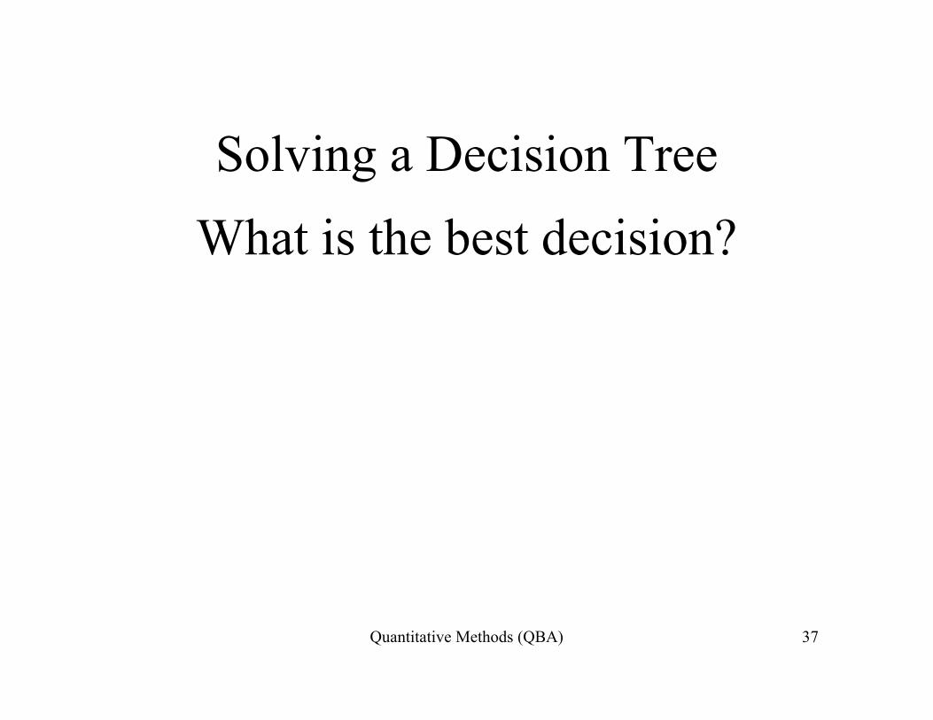
Expected Value• Event node with n mutually exclusive• Event node with n mutually exclusive
events (exactly one of the events will occur)occur).
• Value of event i is Vi
• probability of event i is pi
• Then the expected value of the event node pis EV = p1V1 + p2V2....+ pnVn
Quantitative Methods (QBA) 44

Expected Value
Sometimes you see the “Gamma” symbol for the sum:
1 1 2 2 ...n
n n i ip V p V p V p V 1i
Quantitative Methods (QBA) 45

Expected Value
Note: 0<pi<1 (i=1,2,…,n)and p1 +....+ pn = pi =1p1 pn pi
Quantitative Methods (QBA) 46

Decision Tree
20
= 0 4*(-100)+0 6*100
20
0.4 (-100)+0.6 100

Decision Tree
2020
-10
= 0.4*50+0.6*(-50)
Decision Tree
2020
-10

Decision Tree
2020
-10

EV(Outdoors) > EV(Indoors)EV(Outdoors) > EV(Indoors)
2020
20
-10

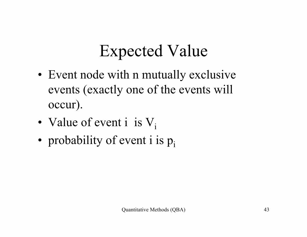
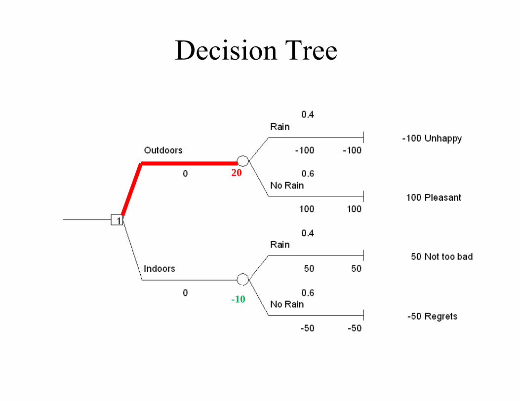
Decision TreeDecision Tree
0.4Rain
-100 UnhappyOutdoors -100 -100
0 20 0.6No Rain
100 Pleasant100 100
d l120 0.4
Rain50 Not too bad
Indoors 50 50
Node values
Indoors 50 50
0 -10 0.6No Rain
-50 Regrets
Quantitative Methods (QBA) 52
-50 -50

Evaluation of Decision Tree0.4
Rain-100 Unhappy
Outdoors -100 -100
0 20 0.6No Rain
100 Pleasant100 100
120 0.4
Rain50 Not too bad
Indoors 50 50Indoors 50 50
0 -10 0.6No Rain
-50 Regrets
Quantitative Methods (QBA) 53
-50 -50

E l ti f D i i TEvaluation of Decision TreeRoll back method: start at terminal nodes andRoll back method: start at terminal nodes and
work from right to left.Compute Expected Value of Event NodesCompute Expected Value of Event NodesChoose Event Node with maximum (or
i i ) EV i D i i N dminimum) EV in Decision NodesThe value of the tree is the EV in the root of
the tree (if values are money it is called the EMV or Expected Money Value)
Quantitative Methods (QBA) 54

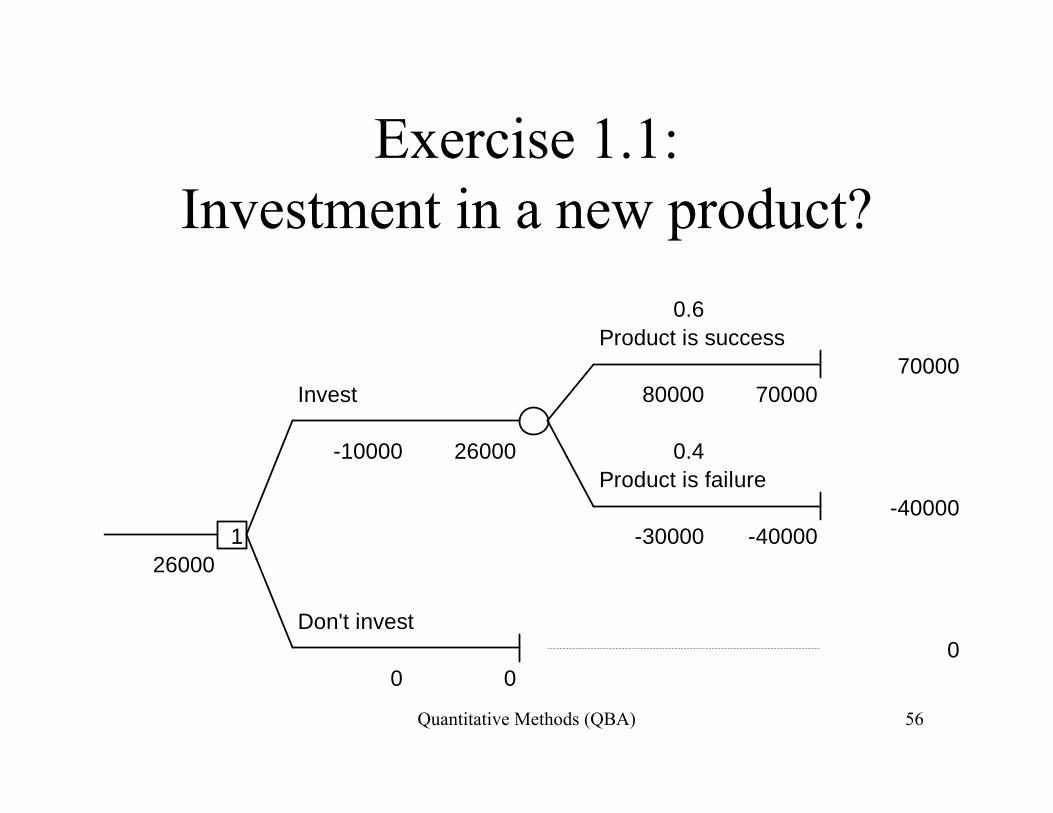
Exercise 1 1:Exercise 1.1: Investment in a new product?
• Investment costs €10 000Investment costs €10.000• Market research
60% €80 000 fi=> 60% success, €80.000 profit40% failure, - €30.000 loss
• Investment cost not yet included in profit.
Quantitative Methods (QBA) 55
Exercise 1 1:Exercise 1.1: Investment in a new product?
0.6Product is success
70000Invest 80000 70000
-10000 26000 0.410000 26000 0.4Product is failure
-400001 -30000 -40000
2600026000
Don't invest0
Quantitative Methods (QBA) 56
0 0

Exercise 1 1:Exercise 1.1: Investment in a new product?
0.6Product is success
70000Invest 80000 70000
-10000 26000 0.410000 26000 0.4Product is failure
-400001 -30000 -40000
26000= 0.6*70000 + 0.4*(-40000)
26000
Don't invest0
Quantitative Methods (QBA) 57
0 0

Exercise 1 1:Exercise 1.1: Investment in a new product?
0.6Product is success
70000Invest 80000 70000
-10000 26000 0.410000 26000 0.4Product is failure
-400001 -30000 -40000
2600026000
Don't invest0
Quantitative Methods (QBA) 58
0 0

• Note that we have not yet discussed risk attitude!
• Investing is risky because we could lose 40000 with a 40% chance
0.6Product is success
with a 40% chance.
70000Invest 80000 70000
-10000 26000 0.410000 26000 0.4Product is failure
-400001 -30000 -40000
2600026000
Don't invest0
Quantitative Methods (QBA) 59
0 0

We will talk about risk attitude (risk averse – risk loving) when we discuss the concept of “utility”.
0.6Product is success
70000Invest 80000 70000
-10000 26000 0.410000 26000 0.4Product is failure
-400001 -30000 -40000
2600026000
Don't invest0
Quantitative Methods (QBA) 60
0 0

Implicit assumption in analysis below:
we are risk indifferent.
0.6Product is success
70000Invest 80000 70000
-10000 26000 0.410000 26000 0.4Product is failure
-400001 -30000 -40000
2600026000
Don't invest0
Quantitative Methods (QBA) 61
0 0

Possible Justifications:
(1) W i k i diff t(1) We are risk indifferent.
(2) We make these kinds of decisions a lot. 0.6
Product is success
( )
70000Invest 80000 70000
-10000 26000 0.410000 26000 0.4Product is failure
-400001 -30000 -40000
2600026000
Don't invest0
Quantitative Methods (QBA) 62
0 0

Multistage Decisions
• So far: single-stage problems
Quantitative Methods (QBA) 63

Multistage Decisions
• So far: single-stage problems
• Choose one decision alternative => outcome• Choose one decision alternative => outcome
Quantitative Methods (QBA) 64

Multistage Decisions
• So far: single-stage problems
• Choose one decision alternative => outcome• Choose one decision alternative => outcome
• Multistage problem: involves sequence of decision alternatives and outcomes
Quantitative Methods (QBA) 65

Multistage Decisions - Example
• Pharmaceutical company concerned with product development on cancer treatment
Quantitative Methods (QBA) 66

Multistage Decisions - Example
• Pharmaceutical company concerned with product development on cancer treatment
• Shall we submit a proposal for government grant of €85 000?of €85,000?
Quantitative Methods (QBA) 67

Multistage Decisions - Example
• Pharmaceutical company concerned with product development on cancer treatment
• Shall we submit a proposal for government grant of €85 000?of €85,000?
• Problem: Writing the proposal costs €5,000
Quantitative Methods (QBA) 68

Multistage Decisions - Example
• Next decision: If we get the grant, should we prepare product 1,2 or 3?
Quantitative Methods (QBA) 69

Multistage Decisions - Example
• Next decision: If we get the grant, should we prepare product 1,2 or 3?
• Products induce different equipment costs.
Quantitative Methods (QBA) 70
Multistage Decisions - Example
• Next decision: If we get the grant, should we prepare product 1,2 or 3?
• Products induce different equipment costs.
• Research and Development (R&D) costs cannot be fully predicted.
Quantitative Methods (QBA) 71

Multistage Decisions - Example
• Next decision: If we get the grant, should we prepare product 1,2 or 3?
• Products induce different equiment costs.
• Research and Development (R&D) costs cannot be fully predicted.
• Best case: low development costs
Quantitative Methods (QBA) 72

Multistage Decisions - Example
• Next decision: If we get the grant, should we prepare product 1,2 or 3?
• Products induce different equipment costs.
• Research and Development (R&D) costs cannot be fully predicted.
• Best case: low development costs
Quantitative Methods (QBA) 73• Worst case: high development costs

Multistage Decisions - Example
Best Case Worst Case
Product Equipment costs
R&D costs
Prob-ability
R&D costs
Prob-ability
Best Case Worst Case
1 4,000 30,000 0.4 60,000 0.62 5,000 40,000 0.8 70,000 0.23 4 000 40 000 0 9 80 000 0 13 4,000 40,000 0.9 80,000 0.1
Quantitative Methods (QBA) 74

Multistage Decision
Tree

-5000

-5000 + 85000

-5000 + 85000 – 4000

-5000 + 85000 – 4000 -60000

-5000 + 85000 – 4000 -60000
= 16000

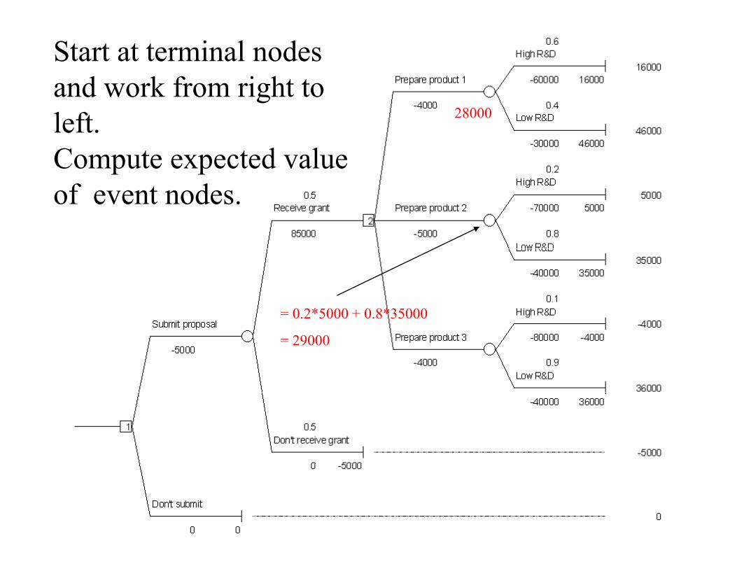
Find best decision byFind best decision by roll back method

Start at terminal nodes and work from right to left.Compute expected value of event nodes.

Start at terminal nodes and work from right to left.Compute expected value = 0.6*16000 + 0.4*46000
of event nodes. = 28000

Start at terminal nodes and work from right to left.Compute expected value
28000
of event nodes.
Start at terminal nodes and work from right to left.Compute expected value
28000
of event nodes.
= 0.2*5000 + 0.8*35000
= 29000

Start at terminal nodes and work from right to left.Compute expected value
28000
of event nodes.
2900029000
0.1*(-4000) + 0.9*36000
= 32000

Choose event node with maximum (or minimum)maximum (or minimum) EV in decision nodes.
28000
2900029000
32000

Choose event node with maximum (or minimum)maximum (or minimum) EV in decision nodes.
28000
2900029000
32000

Choose event node with maximum (or minimum)maximum (or minimum) EV in decision nodes.
28000
2900032000 2900032000
32000

Next step: Again work from right to left. Compute expected value of event nodes.
28000
2900032000 2900032000
32000

Next step: Again work from right to left. Compute expected value of event nodes.
28000
2900032000 2900032000
0.5*32000 + 0.5*(-5000)
= 13500
32000

Next step: Again work from right to left. Compute expected value of event nodes.
28000
2900032000 2900032000
3200013500

Choose event node with maximum (or minimum)maximum (or minimum) EV in decision nodes.
28000
2900032000 2900032000
3200013500

Choose event node with maximum (or minimum)maximum (or minimum) EV in decision nodes.
28000
2900032000 2900032000
3200013500

Choose event node with maximum (or minimum)maximum (or minimum) EV in decision nodes.
28000
2900032000 2900032000
3200013500
13500

Sensitivity Analysis• Sensitivity Analysis: how sensitive is the result for changes in• Sensitivity Analysis: how sensitive is the result for changes in values of parameters?
• Why is this an interesting question?• Why is this an interesting question?
• E.g. the probability to get the grant is usually a rough estimation.estimation.
• We estimated it to be 0.50.
• Do we get a complete different result if it is 0 49 or 0 51?• Do we get a complete different result if it is 0.49 or 0.51?
Quantitative Methods (QBA) 96

Sensitivity Analysis
S i h f hi iSystematic approach of this question:
• We came to the conclusion that it makes sense to submit the proposal if chance to get it is 0 5proposal if chance to get it is 0.5 .
• What is the minimum probability for which it still makes sense to submit the proposal (possibly losing €5000)?sense to submit the proposal (possibly losing €5000)?
Quantitative Methods (QBA) 97

0.6High R&D
16000Prepare product 1 -60000 16000
-4000 28000 0 4-4000 28000 0.4Low R&D
46000-30000 46000
0.2
In general: p
High R&D0.5 5000
Receive grant Prepare product 2 -70000 50002
85000 32000 -5000 29000 0.8Low R&DLow R&D
35000-40000 35000
0.1High R&D
S b it l 4000Submit proposal -4000Prepare product 3 -80000 -4000
-5000 13500-4000 32000 0.9
Low R&D36000
-40000 36000
1 0.513500 Don't receive grant
-50000 50000 -5000
Don't submit0
0 0

0.6High R&D
16000Prepare product 1 -60000 16000
-4000 28000 0 4-4000 28000 0.4Low R&D
46000-30000 46000
0.2
In general: p
High R&D0.5 5000
Receive grant Prepare product 2 -70000 50002
85000 32000 -5000 29000 0.8Low R&DLow R&D
35000-40000 35000
0.1High R&D
S b it l 4000Submit proposal -4000Prepare product 3 -80000 -4000
-5000 13500-4000 32000 0.9
Low R&D360001-p
-40000 36000
1 0.513500 Don't receive grant
-50000 5000
p
0 -5000
Don't submit0
0 0

0.6High R&D
16000Prepare product 1 -60000 16000
-4000 28000 0 4-4000 28000 0.4Low R&D
46000-30000 46000
0.2
In general: p
High R&D0.5 5000
Receive grant Prepare product 2 -70000 50002
85000 32000 -5000 29000 0.8Low R&DLow R&D
35000-40000 35000
0.1High R&D
S b it l 4000
p *32000+(1-p)*(-5000)
Submit proposal -4000Prepare product 3 -80000 -4000
-5000 13500-4000 32000 0.9
Low R&D360001-p
-40000 36000
1 0.513500 Don't receive grant
-50000 5000
p
Compare with 0 0 -5000
Don't submit0
0 0

Sensitivity AnalysisSolve:Solve:
32000*p+ (1 – p)*(-5000) = 0
32000*p = 5000*(1 – p)
32000*p = 5000 – 5000*p
Add on both sides 5000*p
37000*p=5000p
Divide both sides by 37000
=> p = 5/37 = 0 1351
Quantitative Methods (QBA) 102
> p 5/37 0.1351

Sensitivity Analysis
Interpretation:
• For p = 0.1351, we are indifferent between submittingFor p 0.1351, we are indifferent between submitting the proposal or not since it gives us the EMV of zero in both cases.
• For any p higher than 0.1351, we should submit the proposal. p p
Conclusion: the result of the initial assumption p=0.5 is not sensitive to small changes around 0 5
Quantitative Methods (QBA) 103
not sensitive to small changes around 0.5.

Value of InformationValue of Information
Quantitative Methods (QBA) 104

Recall Dilemma: organize party indoors or in garden?
Quantitative Methods (QBA) 105

Recall Dilemma: organize party indoors or in garden?
0.4Rain
-100 UnhappyOutdoors -100 -100
0 20 0.6No Rain
100 Pleasant100 100
120 0.4
Rain50 Not too bad
Indoors 50 50Indoors 50 50
0 -10 0.6No Rain
-50 Regrets
Quantitative Methods (QBA) 106
-50 -50

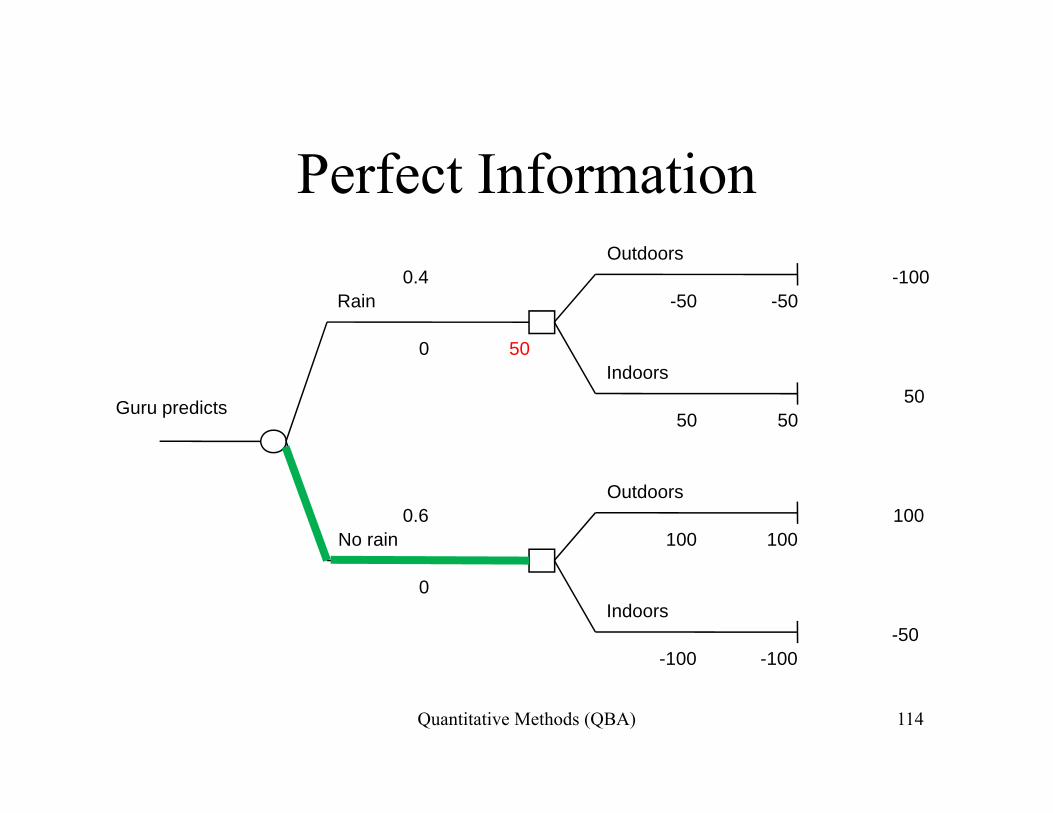
Value of Perfect Information
• 40% of the time rain, 60% no rain. • Guru is able to perfectly predict weatherGuru is able to perfectly predict weather. • Guru tells you 40% of the time: “it will
rain” => rainrain => rain.• Guru tells you 60% of the time: “it will not
i ” irain” => no rain.• Guru is always right. How much would you
Quantitative Methods (QBA) 107be prepared to pay for this information?

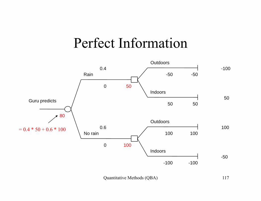
Perfect InformationOutdoorsOutdoors
0.4 -100Rain -50 -50
0Indoors
5050 50
Guru predicts
Outdoors0.6 100
No rain 100 100
0Indoors
-50-100 -100
Quantitative Methods (QBA) 108
100 100

Note that this tree is different from tree without information!
OutdoorsOutdoors0.4 -100
Rain -50 -50
0Indoors
5050 50
Guru predicts
Outdoors0.6 100
No rain 100 100
0Indoors
-50-100 -100
Quantitative Methods (QBA) 109
100 100

Recall: tree without informationRecall: tree without information
0.4Rain
-100 UnhappyOutdoors -100 -100
0 20 0.6No Rain
100 Pleasant100 100
120 0.4
Rain50 Not too bad
Indoors 50 50Indoors 50 50
0 -10 0.6No Rain
-50 Regrets
Quantitative Methods (QBA) 110
-50 -50

Perfect InformationOutdoorsOutdoors
0.4 -100Rain -50 -50
0Indoors
5050 50
Guru predicts
Outdoors0.6 100
No rain 100 100
0Indoors
-50-100 -100
Quantitative Methods (QBA) 111
100 100

Perfect InformationOutdoorsOutdoors
0.4 -100Rain -50 -50
0Indoors
5050 50
Guru predicts
Outdoors0.6 100
No rain 100 100
0Indoors
-50-100 -100
Quantitative Methods (QBA) 112
100 100

Perfect InformationOutdoorsOutdoors
0.4 -100Rain -50 -50
0 50Indoors
5050 50
Guru predicts
Outdoors0.6 100
No rain 100 100
0Indoors
-50-100 -100
Quantitative Methods (QBA) 113
100 100
Perfect InformationOutdoorsOutdoors
0.4 -100Rain -50 -50
0 50Indoors
5050 50
Guru predicts
Outdoors0.6 100
No rain 100 100
0Indoors
-50-100 -100
Quantitative Methods (QBA) 114
100 100

Perfect InformationOutdoorsOutdoors
0.4 -100Rain -50 -50
0 50Indoors
5050 50
Guru predicts
Outdoors0.6 100
No rain 100 100
0Indoors
-50-100 -100
Quantitative Methods (QBA) 115
100 100

Perfect InformationOutdoorsOutdoors
0.4 -100Rain -50 -50
0 50Indoors
5050 50
Guru predicts
Outdoors0.6 100
No rain 100 100
0 100Indoors
-50-100 -100
Quantitative Methods (QBA) 116
100 100
Perfect InformationOutdoorsOutdoors
0.4 -100Rain -50 -50
0 50Indoors
5050 50
Guru predicts
80Outdoors
0.6 100No rain 100 100
= 0.4 * 50 + 0.6 * 100
0 100Indoors
-50-100 -100
Quantitative Methods (QBA) 117
100 100

Value of Perfect Information
Value with perfect information: 80Value without information: 20Value without information: 20Value of perfect information: 80 – 20 = 60
Quantitative Methods (QBA) 118

Value of Perfect Information
Value with perfect information: 80Value without information: 20Value without information: 20Value of perfect information: 80 – 20 = 60
What if Guru is not always right and you get imperfect information?
Quantitative Methods (QBA) 119

Imperfect Information
• Perfect information: Guru is right 100% ofPerfect information: Guru is right 100% of the time.
• Now suppose Guru is not always right, butNow suppose Guru is not always right, but only 65% of the time.
• E.g. after his rain warning it indeed rainsE.g. after his rain warning it indeed rains 65% of the time.
• How much is his information worth?How much is his information worth? • To adress this question we need the notion
“conditional probability”.Quantitative Methods (QBA) 120
conditional probability .

Imperfect Information
Suppose the Guru’s rain warning is only right 65%Suppose the Guru s rain warning is only right 65% of the time. Let R|W mean “It rains after the Guru has given an warning”. P(R|W) = 0.65g g ( | )
Consequence: P(no R|W) = 0.35, i.e. Guru warned for rain but was wrong.g
Assume the probability that it will rain is still 40%. Notation: P(R) = 0.4, P(no R) = 0.6( ) ( )
Suppose Guru warns for rain 45% of the time. Notation: P(W) = 0.45 and P(no W) = 0.55
Quantitative Methods (QBA) 121
( ) ( )

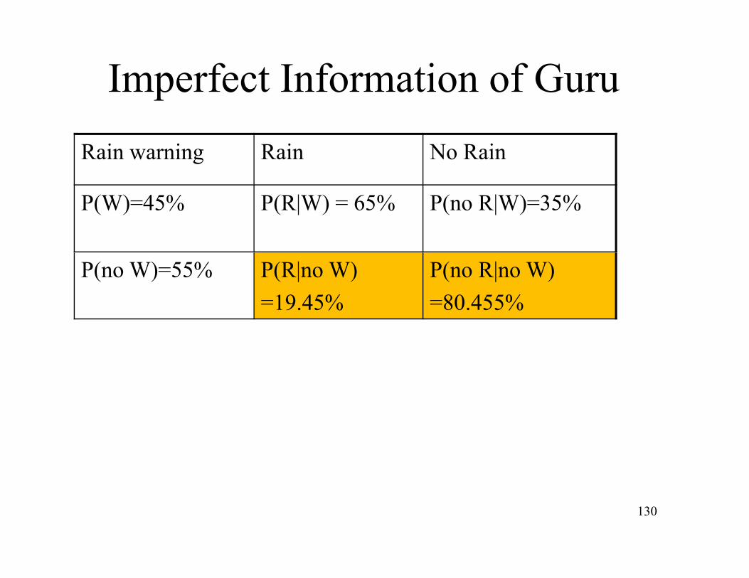
Imperfect Information of Guru Rain warning Rain No Rain
P(W)=45% P(R|W) = 65% P(no R|W)=35%
Quantitative Methods (QBA) 122

Imperfect Information of Guru Rain warning Rain No Rain
P(W)=45% P(R|W) = 65% P(no R|W)=35%
Note: Warning (information) of Guru is imperfectWarning (information) of Guru is imperfect. If it was perfect: P(R|W)=100%. But still valuable information since P(R)=0 4 hence P(R|W)But still valuable information since P(R) 0.4, hence P(R|W)
is larger.Conclusion: Rain probability indeed increases when Guru
Quantitative Methods (QBA) 123
p ywarns.

Imperfect Information of Guru Rain warning Rain No Rain
P(W)=45% P(R|W) = 65% P(no R|W)=35%
Conclusion: Information of Guru is worth something – but how much?how much?
In order to answer this we have to complete table.
Quantitative Methods (QBA) 124

Imperfect Information of Guru Rain warning Rain No Rain
P(W)=45% P(R|W) = 65% P(no R|W)=35%
P(no W)=55%
Quantitative Methods (QBA) 125

Imperfect Information of Guru Rain warning Rain No Rain
P(W)=45% P(R|W) = 65% P(no R|W)=35%
P(no W)=55% P(R|no W)=? P(no R|no W)=?
Recall: P(R) = P(R|W) * P(W) + P(R|no W) * P(no W)
P(R) = 0.4 is given by exercise, rest given by table except P(R|no W)
Quantitative Methods (QBA) 126
-> solve equation for P(R|no W)

Imperfect Information of Guru Rain warning Rain No Rain
P(W)=45% P(R|W) = 65% P(no R|W)=35%
P(no W)=55% P(R|no W)=? P(no R|no W)=?
Recall: P(R) = P(R|W) * P(W) + P(R|no W) * P(no W)
Maybe easier: insert all values we know and then solve for P(R|no W)
Quantitative Methods (QBA) 127

Imperfect Information of Guru Rain warning Rain No Rain
P(W)=45% P(R|W) = 65% P(no R|W)=35%
P(no W)=55% P(R|no W)=? P(no R|no W)=?
Recall: P(R) = P(R|W) * P(W) + P(R|no W) * P(no W)
0.4 = 0.65 * 0.45 + P(R|no W) * 0.550.4 = 0.2925 + P(R|no W) * 0.55
128
0.1075 = P(R|no W) * 0.55 0.19545 = P(R|no W)

Imperfect Information of Guru Rain warning Rain No Rain
P(W)=45% P(R|W) = 65% P(no R|W)=35%
P(no W)=55% P(R|no W)=? P(no R|no W)=?
From P(R|no W) = 0.19545 we get P(no R|no W) = 1 0 19545 = 0 80455we get P(no R|no W) = 1 - 0.19545 = 0.80455
129
Imperfect Information of Guru Rain warning Rain No Rain
P(W)=45% P(R|W) = 65% P(no R|W)=35%
P(no W)=55% P(R|no W)=19.45%
P(no R|no W)=80.455%
130

0 .6 5R a in
-1 0 0O u td o o rs -1 0 0 -1 0 0
0 -3 0 0 .3 50 3 0 0 3 5N o ra in
0 .4 5 1 0 0W a rn in g 1 0 0 1 0 0
20 1 5 0 .6 5
R a inR a in5 0
In d oo rs 5 0 5 0
0 1 5 0 .3 5N o ra in
5 0-5 0-5 0 -5 0
40 .24 5 0 .1 9 5 5R a in
-1 0 0O u td o o rs -1 0 0 -1 0 0
0 6 0 .9 0 .8 0 4 5N o ra in
0 .5 5 1 0 0N o W a rn in g 1 0 0 1 0 0
10 60 .9 0 .1 9 5 5
R a in5 0
In d oo rs 5 0 5 0
0 -3 0 .4 5 0 .8 0 4 5N o ra in
-5 0-5 0 -5 0

Imperfect Information0.65
Rain-100
O utdoors -100 -100
0 -30 0.35No ra in
0.45 100W arn ing 100 100
20 15 0.65
Rain50
Indoors 50 50
0 15 0 350 15 0.35No ra in
-50-50 -50
40.245 0.1955Rain
-100O utdoors -100 -100
0 60.9 0.8045No rainNo ra in
0 .55 100No W arning 100 100
10 60.9 0.1955
Rain50
Indoors 50 50
0 -30.45 0.8045No ra in
-50-50 -50
Expected value without information: EMV=20
Expected value with sample (imperfect) information: 40 245Expected value with sample (imperfect) information: 40.245
Expected value of sample information: 40.245 – 20 = 20.245
Interpretation: 20.245 = Maximum price we are willing to pay the Guru.
Quantitative Methods (QBA) 132
Interpretation: 20.245 Maximum price we are willing to pay the Guru.

Another example: Should we build aAnother example: Should we build a large or small factory?
Problem: • introduce a new product• introduce a new product • don’t know yet whether demand will be high or low• if demand is high -> large factory might be optimalif demand is high large factory might be optimal • if demand is low -> small factory might be optimal
Quantitative Methods (QBA) 133

Another example: Should we build aAnother example: Should we build a large or small factory?
Construction costs: Large Factory €25 MillionSmall Factory €15 Million
Factory Size High Demand Low Demand
Large 175 95
Small 125 105
Probability 70% 30%Probability 70% 30%
Estimated total Revenues (in million €)
Quantitative Methods (QBA) 134

Decision Tree without Survey0.7
High demand150
Large plant 175 150
-25 126 0 325 126 0.3Low demand
7095 70
1126 0 7126 0.7
High demand110
Small plant 125 110
-15 104 0.3Low demand
90105 90
Quantitative Methods (QBA) 135

Estimated Results of Survey
P b bilit S Hi h D d L D dProbability Survey High Demand Low Demand
67% Favourable 90% 10%33% U f bl 30% 0%33% Unfavourable 30% 70%
Quantitative Methods (QBA) 136

0.9High demand
150Large plant 175 150
Decision Tree with Survey -25 142 0.1
Low demand0.67 70
Favourable 95 701
0 142 0.9High demand
with Survey
High demand110
Small plant 125 110
-15 108 0.1Low demand
90Conduct survey 105 90
1126.82 0 126.82 0.3
High demand150
Large plant 175 150
-25 94 0.7Low demand
0.33 70Unfavourable 95 70
20 96 0 30 96 0.3
High demand110
Small plant 125 110
-15 96 0.7Low demand
Quantitative Methods (QBA) 137
90105 90
0.65Rain
-100O utdoors -100 -100
0 -30 0.35No ra in
0.45 100W arning 100 100
20 15 0.65
Rain50
Indoors 50 50
0 15 0.35No ra in
-50-50 -50
40.245 0.1955Rain
-100O utdoors -100 -100
0 60.9 0.8045No ra in
0.55 100No W arning 100 100
10 60.9 0.1955
Rain50
Indoors 50 50
0 -30.45 0.8045No ra in
-50-50 -50
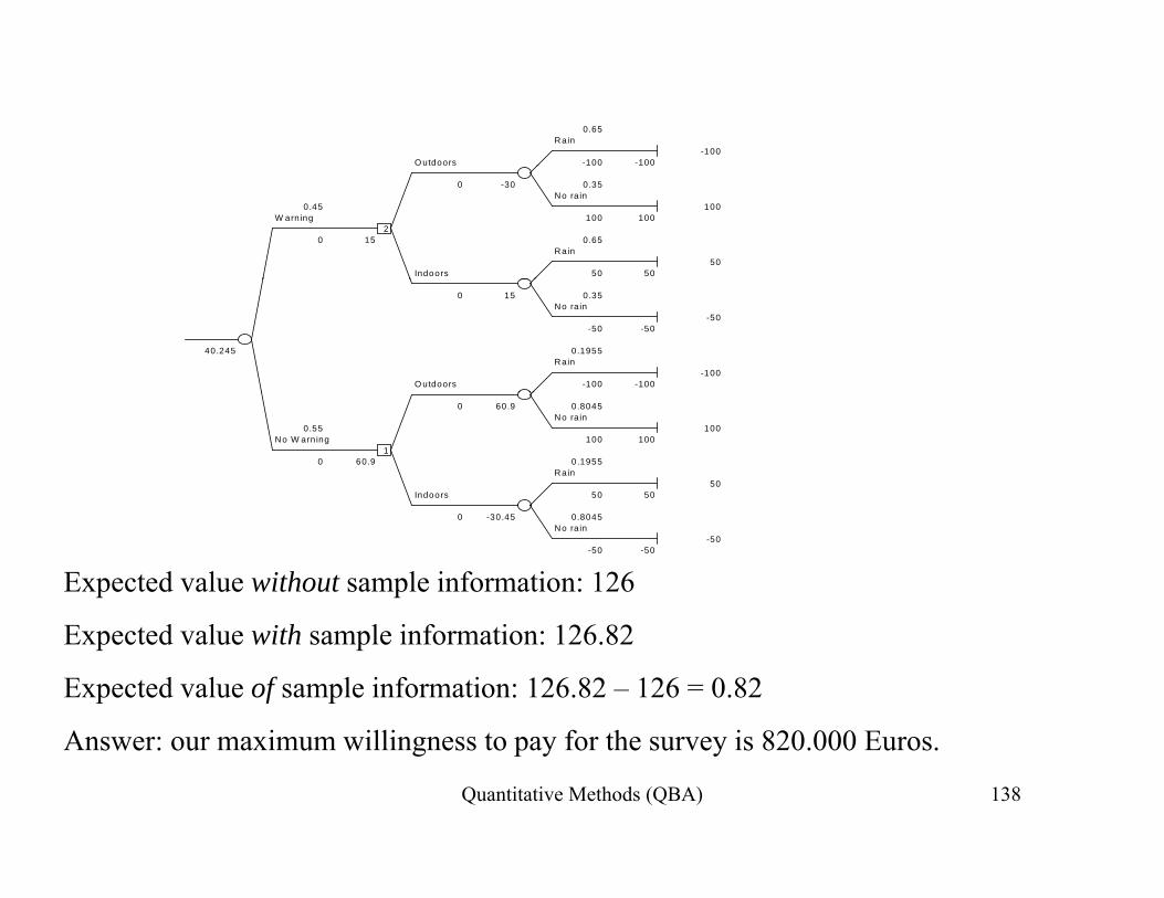
Expected value without sample information: 126
Expected value with sample information: 126.82
Expected value of sample information: 126.82 – 126 = 0.82
A i illi f h i 820 000 E
Quantitative Methods (QBA) 138
Answer: our maximum willingness to pay for the survey is 820.000 Euros.

Expected Money Value -is this always a good criterion for
choice under risk?choice under risk?
Quantitative Methods (QBA) 139

Example –
0.5
payoff in million EurosGood results
150Buy Company A 250 150
-100 60 0.5Less good results
-3070 -30
160 0.5
Good results70
Buy Company B 170 70
-100 55 0.5Less good resultsLess good results
40140 40

Taking risksC P ff P ff EMVCompany Payoff Payoff EMVA 150 -30 60B 70 40 55Probability 0.5 0.5
• Should we buy company A or B?
Quantitative Methods (QBA) 141

Taking risksC P ff P ff EMVCompany Payoff Payoff EMVA 150 -30 60B 70 40 55Probability 0.5 0.5
• Should we buy company A or B?
E i l i Sh ld l bl A B?• Equivalent question: Should we play gamble A or B?
Quantitative Methods (QBA) 142

Taking risksC P ff P ff EMVCompany Payoff Payoff EMVA 150 -30 60B 70 40 55Probability 0.5 0.5
• Nobody would hesitate to play gamble B.
Quantitative Methods (QBA) 143

Taking risksC P ff P ff EMVCompany Payoff Payoff EMVA 150 -30 60B 70 40 55Probability 0.5 0.5
• Nobody would hesitate to play lottery B.
G bl A l i d i k f l i €30 illi• Gamble A less attractive due to risk of losing €30 million.
Quantitative Methods (QBA) 144

Taking risksC P ff P ff EMVCompany Payoff Payoff EMVA 150 -30 60B 70 40 55Probability 0.5 0.5
• Nobody would hesitate to play gamble B.
G bl A l i d i k f l i €30 illi• Gamble A less attractive due to risk of losing €30 million.
• Note EMV(A) > EMV(B)
Quantitative Methods (QBA) 145

Taking risksC P ff P ff EMVCompany Payoff Payoff EMVA 150 -30 60B 70 40 55Probability 0.5 0.5
Conclusion: EMV doesn’t reflect how we feel about risk!
Quantitative Methods (QBA) 146

Utility Function
• Fundamental premise: people choose the lt ti th t h t th hi h t t d lalternative that has not the highest expected value
but the highest expected utility
• Assume utility function U that assigns a numerical measure to the satisfaction associated with different outcomes.
H d h tilit f ti l k lik ?• How does such a utility function look like?

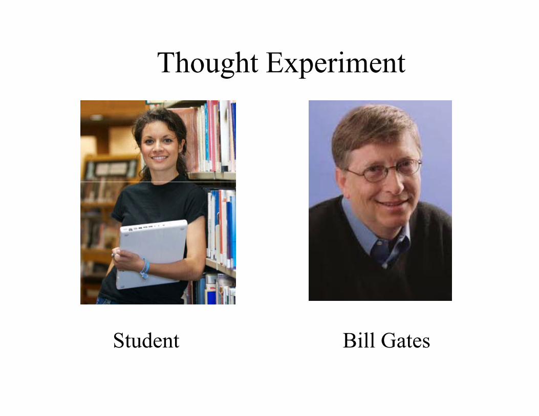
Thought ExperimentGive the following two persons €100 as a gift.
Who’s happiness will increase more?
Thought Experimentg p
Student Bill GatesStudent Bill Gates

Thought ExperimentFrequent observation: The more money we have, the less our happiness increases with additionalthe less our happiness increases with additional money.

A Concave Utility Function

Thought Experiment• Warning: utility function is not always concave!
• We will see that it depends on our attitude towards risk, i.e. whether we risk-avert or risk-loving.

Utility Function• Note: utility is “dimensionless”, i.e. there is no unit such as $ kg cmunit such as $, kg, cm.
• This function assigns numbers to outcomes. g
• The higher the number, the more we like the outcomeoutcome.
• Without loss of generality, assume these numbers are between 0 and 1
• Otherwise substract minimum and divide by• Otherwise substract minimum and divide by the maximum

Utility FunctionExample:
Assume Anna says her utility level of money in Euros are
U(100) = 10, U(0) = 5, U(-50) = 1

Utility FunctionU(100) = 10, U(0) = 5, U(-50) = 1

Utility FunctionU(100) = 10, U(0) = 5, U(-50) = 1
If we substract 1 (the minimum) from every value we get g
U(100) = 9, U(0) = 4, U(-50) = 0

Utility FunctionU(100) = 10, U(0) = 5, U(-50) = 1
If we substract 1 (the minimum) from every value we get g
U(100) = 9, U(0) = 4, U(-50) = 0
Finally, divide all values by 9 to get
U(100) = 1 U(0) = 4/9=0 44 U( 50) = 0U(100) = 1, U(0) = 4/9=0.44, U(-50) = 0

Utility FunctionNote:
• what we did here was to convert utility into a more convenient form
• comparable as e.g. when you convert prices from dollars to eurosfrom dollars to euros
Utility Function
How do we construct a person’s utility function (preference)?

Example: Gambling or not?
$0 Gamble0.5
$50.0000.5
Don’t gamble?
Don t gamble
What is the minimum amount we have to pay Jane to make her p ywalk away from the gamble?

Example: Gambling or not?
$0 Gamble0.5
$50.0000.5
Don’t gamble?
Don t gamble
Janes’ certainty equivalent for the gambleg
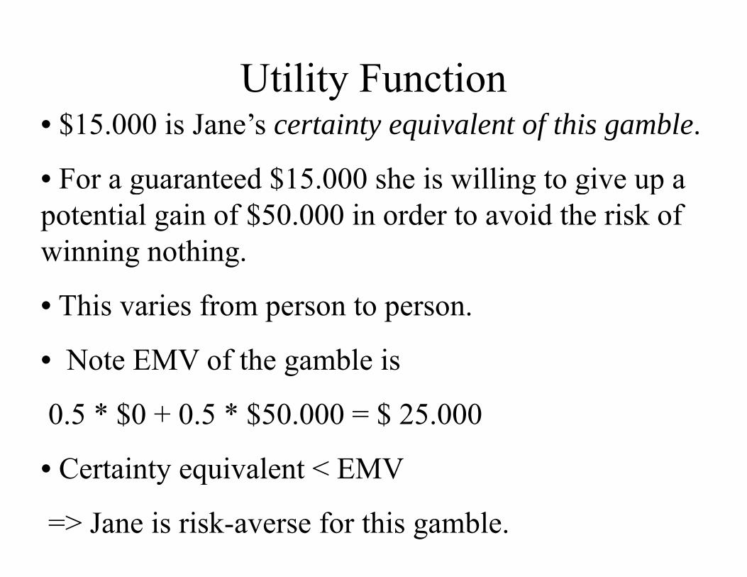
Utility Function• $15.000 is Jane’s certainty equivalent of this gamble.
• For a guaranteed $15 000 she is willing to give up a• For a guaranteed $15.000 she is willing to give up a potential gain of $50.000 in order to avoid the risk of winning nothingwinning nothing.
• This varies from person to person.
• Note EMV of the gamble is
0.5 * $0 + 0.5 * $50.000 = $ 25.000
• Certainty equivalent < EMV• Certainty equivalent < EMV
=> Jane is risk-averse for this gamble.

Utility Perspective
U($0) =0Gamble0.5
U($50.000) =10.5EU=0.5
Don’t gamble U($15.000)=?Don t gamble ( )

Utility Perspective
U($0) =0Gamble0.5
U($50.000) =10.5EU=0.5
Don’t gamble U($15.000)=0.5Don t gamble ( )

Utility Function
To find more values of U repeat gamble questionsTo find more values of U repeat gamble questions.
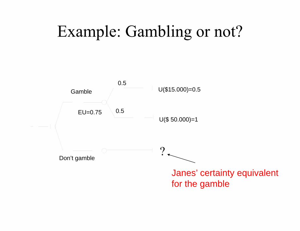
Example: Gambling or not?
U($15.000)=0.5 Gamble0.5
U($ 50.000)=1 0.5EU=0.75
Don’t gamble?
Don t gamble
Janes’ certainty equivalent for the gambleg

Example: Gambling or not?
U($15.000)=0.5 Gamble0.5
U($ 50.000)=1 0.5EU=0.75
Don’t gambleU($27.000)=0.75
Don t gamble

Example: Gambling or not?
U($15.000)=0.5 Gamble0.5
EMV = 0 5*$15 000 +0 5*$50 000
U($ 50.000)=1 0.5EU=0.75
EMV = 0.5 $15.000 +0 .5 $50.000= $32.500
Don’t gambleU($27.000)=0.75
Don t gamble

Example: Gambling or not?
U($15.000)=0.5 Gamble0.5
EMV = 0 5*$15 000 +0 5*$50 000
U($ 50.000)=1 0.5EU=0.75
EMV = 0.5 $15.000 +0 .5 $50.000= $32.500
Don’t gambleU($27.000)=0.75
Don t gamble
Certainty equivalent < EMV -> risk averse risk averse

Utility Curve for JaneUtility Curve for Jane Concave => risk-avoider

Risk Aversion• Jane would be a risk averse person when she is risk averse for any gamblerisk averse for any gamble.
• In formulae: gamble with probability p to win g p y pamount V1 and with probability 1-p to win V2.
EMV f thi bl * V (1 )* V• EMV of this gamble = p* V1 (1p)* V2
• Certainty equivalent of this gamble is C.Certainty equivalent of this gamble is C.
• Then C < p* V1 (1p)* V2 means that she is i krisk averse.

Utility Function
How does the utility function of a risk-seeker look like?

Utility FunctionExample: Mark’s preference between $30 000 andMark s preference between $30.000 and $40.000
Receipe:
• Assign utility 0 to the lowest ( $30 000 )• Assign utility 0 to the lowest ($30.000 )
• Assign utility 1 to the highest ($40.000 )
• To find out about in-between values we ask Mark questions about gamblesMark questions about gambles.

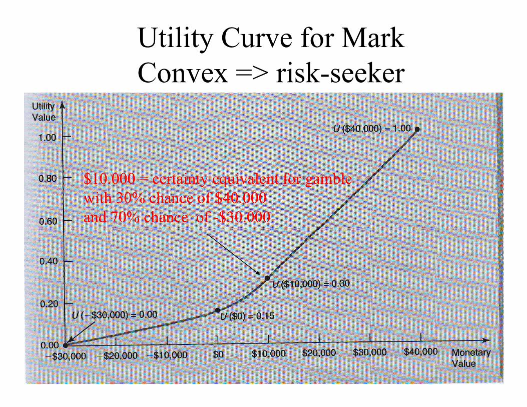
Utility Curve for Mark Convex => risk-seekerConvex => risk-seeker
Utility Curve for Mark Convex => risk-seekerConvex => risk-seeker
$10 000 = certainty equivalent for gamble$10.000 = certainty equivalent for gamble with 30% chance of $40.000 and 70% chance of -$30.000

Utility Curve for Mark Convex => risk-seekerConvex => risk-seeker
BBecause
0.3*U(highest) + 0.7*U(lowest)
= 0.3*1 + 0.7*0
= 0.3

Utility Curve for Mark Convex => risk-seekerConvex => risk-seeker
certainty equivalent for gamble = $10 000certainty equivalent for gamble = $10.000 EMV = -$9.000

Utility Curve for Mark Convex => risk-seekerConvex => risk-seeker
EMV<0 but still we have to pay MarcEMV<0 but still we have to pay Marc
to walk away from the gamble!

Utility FunctionIn general, gamble
with chance p to win highest outcome ($40.000 ) chance 1-p to win lowest outcome (-$30.000 )p ( )
Expected utility:
p*U(highest) + (1-p)*U(lowest)
= p*1 + (1 p)*0= p*1 + (1-p)*0
= p

Utility Function• Expected utility of gamble between lowest and highest outcome = phighest outcome = p.
If Mark tells us that U($0)=0.15( )
$0 is certainty equivalent of gamble which wins the highest payoff with 15% chance the lowest withthe highest payoff with 15% chance, the lowest with 85% chance.
Mark is risk-seeking.

Utility Function
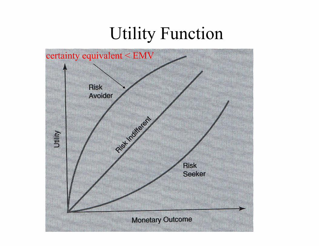
Utility Functioncertainty equivalent < EMV

Utility Function
certainty equivalent > EMV

E t d tilitUtility Function
Expected utilitycertainty equivalent
= EMV= EMV

Risk averse: diminishing marginal utility
Ri k t l t t i l tilitRisk neutral: constant marginal utility
Risk seeking: increasing marginal utility

Example: Should Mark Invest in New Business?New Business?

Example: Should Mark Invest in New Business?
Payoffs in DollarsNew Business?
0 2$ 40 000
$10 000
invest
$ -4000
0.2
0.3
0 5
$ 0$ -30 000
$ 0.5
Do not invest$ 0
$ 0

Example: Should Mark Invest in New Business?
Payoffs in DollarsNew Business?
Comparing EMV of his options => no investment 0 2
$ 40 000
$10 000
invest
$ -4000
0.2
0.3
0 5
$ 0$ -30 000
$ 0.5
Do not invest$ 0
$ 0

Expected utilityExample: Should Mark Invest in
New Business?p yNow instead of monetary payoffs consider his utility
which reflects his risk attitude
New Business?
– which reflects his risk attitude.
0 2$ 40 000
$10 000
invest
$ -4000
0.2
0.3
0 5
$ 0$ -30 000
$ 0.5
Do not invest$ 0
$ 0

Example: Should Mark Invest in New Business?New Business?
1 = highest outcome
$ 40 000invest
0.2
0 3$ 10 000
$ -30 000
0.3
0.5
$ 0
Do not invest

Example: Should Mark Invest in New Business?New Business?
0 = lowest outcome$ 40 000invest
0.2
0.3$ 10 000
$ -30 0000.5
Do not invest
$ 0
Do not invest

Example: Should Mark Invest in New Business?New Business?
0.3$ 40 000invest
0.2
$ 10 000
$ -30 000
invest0.3
0.5
0.15$
$ 0
Do not invest
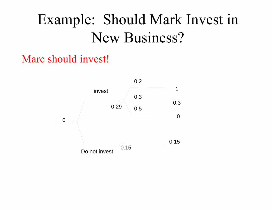
Example: Should Mark Invest in New Business?New Business?
Marc should invest!
1invest
0.2
0
0.3
0
invest
0.29
0.3
0.5
0
0.15
Do not invest0.15

Warnings Using Utility Theory• Each person’s has his or her own utility function.
• It could change over time, e.g. with getting older or richer.
• A person’s utility function can change with different rangedifferent range.
• E.g. most people are risk seeking when potential losses are small.
• This changes when potential losses get larger!• This changes when potential losses get larger!

Warnings Using Utility Theory=> Consider utility function only over relevant range of monetary values of a specific problemrange of monetary values of a specific problem.