Quantitative BasicsDescriptive Statistics

Class 2a

For Tomorrow

• Read, then write two abstracts for articles (not lit reviews) related to your study. – Taken from list for today.

• Read entire article• write summary• compare w/ abstract if there is one• Email to me as soon as you finish

• Read: Hash, P. M. (2010). Preservice Classroom Teacher’s Attitudes toward Music in the Elementary Curriculum. Journal of Music Teacher Education, 19(2), 6-24.

• All current abstracts from the JRME and Update.

Writing an Abstract

• Include an APA citation• Accurate & dense w/

information• Nonevaluative (not a

review)• Coherent, concise,

readable. Use active voice– Highlight most important

aspects

• 150-200 words. (Use word count tool)

1. Purpose of the study2. Participants (subjects)

& their important characteristics

3. Methodology (what the researcher[s] did)

4. Basic findings5. Conclusions &

Implications

Sample 1• This study examined performance anxiety (PA) among middle school vocal

soloists. Participants included male (n = 63) and female (n = 221) middle school students (N = 284) participating in an all-district solo and ensemble festival. Students completed the Smith Performance Anxiety Inventory (SPAI) immediately following their performance. This survey consisted of 15-closed response questions measuring various physical and emotional phenomena on a seven-step Likert scale. Total SPAI scores indicate that 72% (n = 204) of participants reported moderate to high levels of anxiety and that these students experienced trembling, sweaty palms, and difficulty concentrating at significantly higher levels (p < .01) than other responses measured by the SPAI. Data also indicated that among students that experienced moderate to high levels of PA (n = 204), 86% (n = 175) were female. Recommendations for managing PA include 1) openly discussing PA among students, 2) videotaping performance for self-assessment, and 2) simulating the performance environment many times before the event.

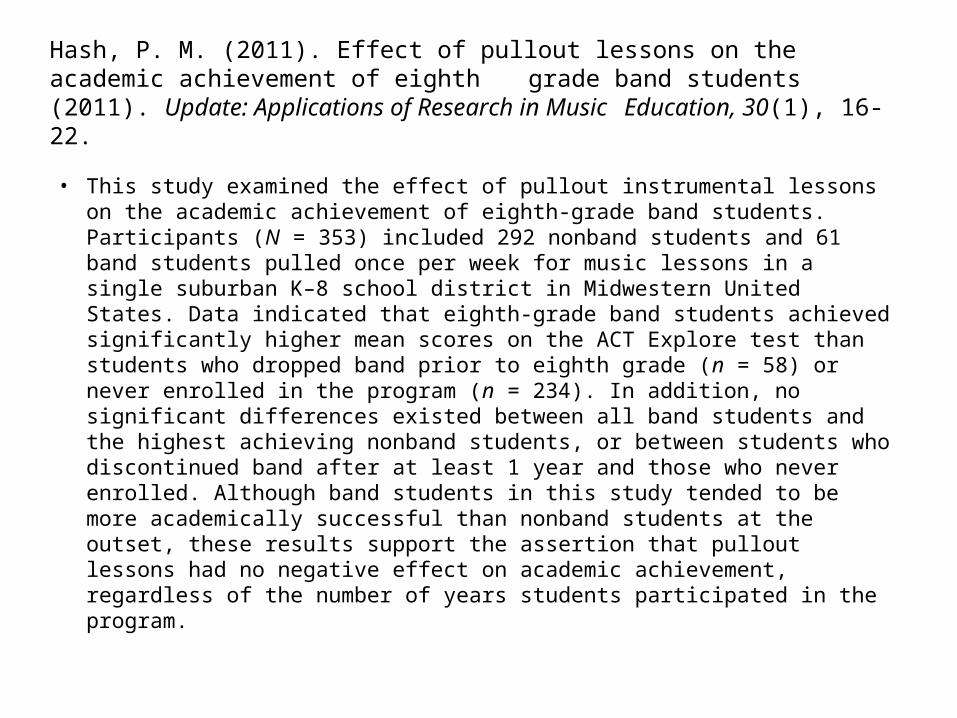
Hash, P. M. (2011). Effect of pullout lessons on the academic achievement of eighth grade band students (2011). Update: Applications of Research in Music Education, 30(1), 16-22.

• This study examined the effect of pullout instrumental lessons on the academic achievement of eighth-grade band students. Participants (N = 353) included 292 nonband students and 61 band students pulled once per week for music lessons in a single suburban K–8 school district in Midwestern United States. Data indicated that eighth-grade band students achieved significantly higher mean scores on the ACT Explore test than students who dropped band prior to eighth grade (n = 58) or never enrolled in the program (n = 234). In addition, no significant differences existed between all band students and the highest achieving nonband students, or between students who discontinued band after at least 1 year and those who never enrolled. Although band students in this study tended to be more academically successful than nonband students at the outset, these results support the assertion that pullout lessons had no negative effect on academic achievement, regardless of the number of years students participated in the program.

Quantitative Basics

Experimental & Surveys

Samples of individuals/entities

• Sample vs. population– Some vs. All– Examples where entire population could be sampled?

• Relationship between sample specificity and generalizability

• Representative sample– Captures relevant and essential characteristics of the

population– What about a sample of teachers? What should the

sample look like?

Sampling Methods• Systematic

– Random start and sampling interval• i.e., Randomly select pages from IHSA directory• choose every ? Name (random number b/w 1-X)

• Convenience– not as valuable but frequent in ed. research – why?

• i.e., intact classes, pre-service teachers from one institution, conference session attendees

• Purposive– Participants fit a particular profile (female band directors

in small towns)– Exclude those who do not fit profile– Often consists of volunteers (problematic)

Types of Samples• Simple Random

– Everyone has equal chance of selection– Reduce systematic bias – error created by sampling method– Phone book, MENC membership list (But??)

• Stratified Random– Similar proportions between sample and population

• Gender, race, age, instrument, etc.• Cluster Random

– Groups rather than individuals• i.e., classes or ensembles in CPS• Then groups can be assigned randomly

– Two-stage random - groups then individuals• i.e., choose classes then assign individual students or groups

to control or treatment group

Sample Size• As large as possible given reasonable expenditure of

time and energy– Most likely to get significant results– More statistically powerful (more likely to find a significant

difference b/w groups)• Sample size relative to:

– the size of population (50 Cook Co. band directors vs. 50 band students throughout US)

– variability within population (years of teaching, gender, etc.)– sampling method (need a large enough pool from which to

draw)– study design (qualitative vs. quantitative)

Types of Data Analysis

• Descriptive– Describes data

• Relational (correlation)– Relationships b/w variables within data

• Differences (inferential statistics)– b/w groups

Measurement ScalesLevels of Measurement

• [NOIR]• Nominal

– Categorical, frequency counts (gender, color, yes/no, etc.)• Ordinal

– Rank-order (Contest Ratings, Likert data??)• Interval

– Continuous scale with consistent distances between points. No meaningful absolute zero (test scores, singing range, temperature, knowledge).

• Ratio– Continuous scale with consistent distances between points and an

absolute zero (decibels, money) • N-choir robes; O – div. 1 at contest; I – 96/100 score; R – festival

score twice as high as last year.

Other Terms

• Reliability = Consistency– Test/retest (regardless of yr., location, etc.)– Interrater (every judge the same)

• Validity = the extent to which an assessment or survey measures what they purport to measure

• Independent Variable – factors manipulated by researcher • Dependent Variable – the test to determine outcome• Significant – Results did not occur by chance. Based on

statistical calculation – not opinion.

Descriptive Statistics

Basics

• Descriptive stats describe population– Central Tendency • Mean (M)• Mode (Mo)• Median (Mdn)

– Variability• Range• Variance• Standard Deviation (SD)

Visual Summaries of Data • Frequencies

• Histogram– Versus a bar graph?

• Bar graph = categorical data, Histogram = quantitative/continuous data

Rank Degree of agreement Number

1 Strongly agree 20

2 Agree somewhat 30

3 Not sure 20

4 Disagree somewhat 15

5 Strongly disagree 15

Central Tendency

• Mean– Sum of all scores divided by number of scores (average)– X --- single score (your test grade)– --- sum (add it all up!)– X --- mean (class average on test)– N or n --- number of individuals/entities (number of people

in class)• X = X/n

• Mode– Most frequently occurring

• Median– Point at which half fall below, half fall above

Variability (spread)• Range

– Distance between lowest and highest score (H-L=R)• Variance

– A measure of the dispersion (spread) of a set of scores. – For the population = The sum of the squared deviations from the

mean/N (number of scores)– For a sample = The sum of the squared deviations from the

mean/n-1 (number of scores minus 1).– Previous formula underestimates the variance in a sample.

Think of -1 as a correction– Abstract – but good for comparing groups on similar

characteristics– Needed to find SD

5681011

Variance Problem – Population http://www.calculatorsoup.com/calculators/statistics/descriptivestatistics.php

• Data set: 5, 6, 8, 10, 11.• Calculate the Mean• Subtract the mean from each score.• Square all the numbers that you obtained from subtracting

each set number by the mean (2 neg. make a pos.):• Add the results• Divide the sum of the numbers by the number of numbers in

the set minus 1.• The variance for the example set of numbers is ?.

SolutionData -M = squared

5 8 -3 9 6 8 -2 4 8 8 0 0

10 8 2 4 11 8 3 9

∑=40/M=8 26/5-1(4) Var = 9.2

Standard Deviation

– A single number which describes the entire distribution of scores in terms of a relationship to the mean. SD=Average distance from the mean expressed in actual units (points in a test, 1-7 scale on a survey)• SD = Square Root of [(X-X)2/n] or [n-

1] (variance)• SD score vs. SD unit (coming up)

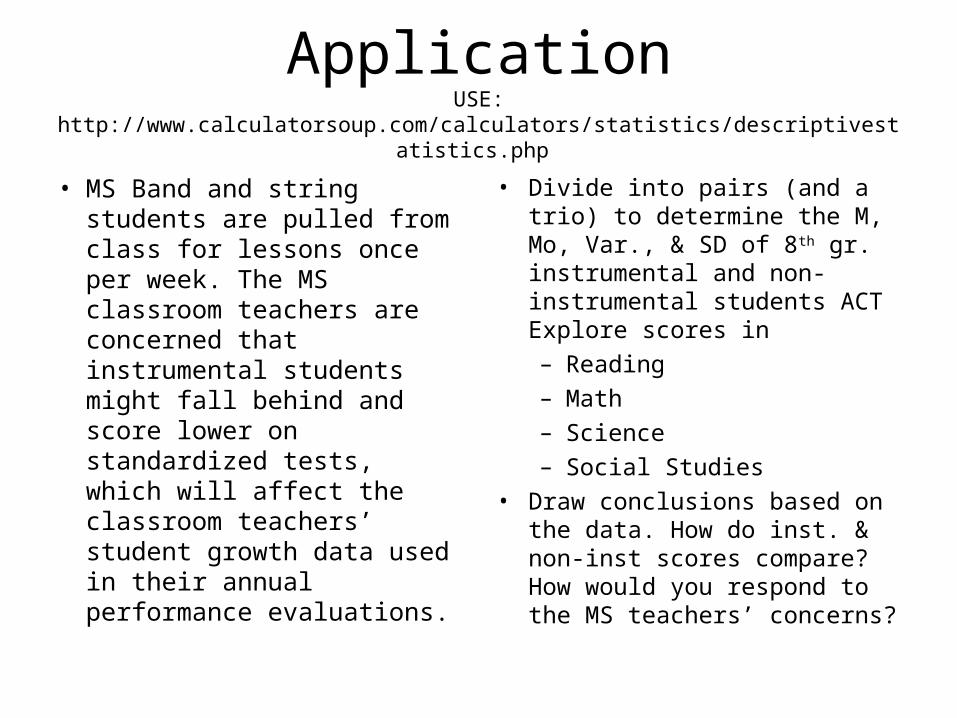
ApplicationUSE: http://www.calculatorsoup.com/calculators/statistics/descriptivestatistics.php

• MS Band and string students are pulled from class for lessons once per week. The MS classroom teachers are concerned that instrumental students might fall behind and score lower on standardized tests, which will affect the classroom teachers’ student growth data used in their annual performance evaluations.

• Divide into pairs (and a trio) to determine the M, Mo, Var., & SD of 8th gr. instrumental and non-instrumental students ACT Explore scores in– Reading– Math– Science– Social Studies

• Draw conclusions based on the data. How do inst. & non-inst scores compare? How would you respond to the MS teachers’ concerns?

Normal Curve/Distribution

Altogether.. describes the shape of a distributionMore on distributions..

• Normal Curve (bell curve)– Most scores clustered at the middle with fewer scores falling

at the extreme highs and lows• Skewness - When the scores tend to bunch up…

• …on the HIGH END = Negative Skew = less than -1• …on the LOW END = Positive Skew = greater than +1

• Kurtosis - When the distribution is…• …PEAKED = positive kurtosis = leptokurtic = greater than +1 or +2

depending on who you ask…• …SMALLER PEAK (flatter) THAN A NORMAL CURVE = negative kurtosis =

platykurtic = less than -1

• Bi-Modal– When there are two humps in the curve, more than one mode

• Kurtosis – shape– platykurtic – leptokurtic

-1 to +1 = a near normal curve

Skewed (positively)

More on the normal curve and variability...

• Theoretical “perfect” curve. Never happens in actual research– Mean, median, mode are equal– 50% of scores lie above mean, 50% lie below– 68.4% of scores are between one SD above the

mean and one SD below the mean– 95% of the scores are within two SD’s above

and below the mean– 99.7% of the scores are within three SD’s

above and below the mean

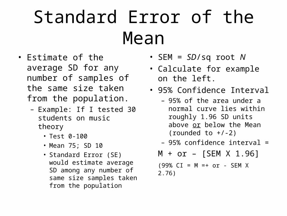
Standard Error of the Mean

• Estimate of the average SD for any number of samples of the same size taken from the population.– Example: If I tested 30

students on music theory• Test 0-100• Mean 75; SD 10• Standard Error (SE) would

estimate average SD among any number of same size samples taken from the population

• SEM = SD/sq root N• Calculate for example on

the left.• 95% Confidence Interval

– 95% of the area under a normal curve lies within roughly 1.96 SD units above or below the Mean (rounded to +/-2)

– 95% confidence interval =

M + or – [SEM X 1.96] (99% CI = M =+ or - SEM X 2.76)

Confidence Limits/Intervalhttp://www.mccallum-layton.co.uk/stats/ConfidenceIntervalCalc.aspx

• Attempts to define range of true population mean based on Standard Error estimate.

• Confidence level– 95% chance vs. 99% chance

• Confidence Limits– 2 numbers that define the range

• Confidence Interval– The range b/w confidence limits

• On surveys– http://www.surveysystem.com/sscalc.htm#two