Quantitative assessment of securitisation deals · · 2011-01-03EURANDOM PREPRINT SERIES 2010-045...

EURANDOM PREPRINT SERIES2010-045

Quantitative assessment ofsecuritisation deals

Henrik Jonsson and Wim SchoutensISSN 1389-2355

1

Quantitative assessment of securitisation deals

Authors: Henrik Jonsson1 and Wim Schoutens2

October 21, 2010

1 Postdoctoral Research Fellow, EURANDOM, Eindhoven, The Netherlands. E-mail:

[email protected] Research Professor, Department of Mathematics, K.U.Leuven, Leuven, Belgium. E-mail: [email protected]

Acknolwledgement:

The presented study is part of the research project “Quantitative analysis and analytical methods

to price securitisation deals”, sponsored by the European Investment Bank via its university

research sponsorship programme EIBURS. The authors acknowledge the intellectual support

from the participants of the previously mentioned project.

Copyright © 2010 Henrik Jonsson and Wim Schoutens

Table of Contents

Preface vii

1 Introduction to Asset Backed Securities 1

1.1 Introduction . . . . . . . . . . . . . . . . . . . . . . . . . . . . . . . . . . . . . . . 1

1.2 Asset Backed Securities Features . . . . . . . . . . . . . . . . . . . . . . . . . . . 1

1.2.1 Asset Classes . . . . . . . . . . . . . . . . . . . . . . . . . . . . . . . . . . 1

1.2.2 Key Securitisation Parties . . . . . . . . . . . . . . . . . . . . . . . . . . . 2

1.2.3 Structural Characteristics . . . . . . . . . . . . . . . . . . . . . . . . . . . 3

1.2.4 Priority of Payments . . . . . . . . . . . . . . . . . . . . . . . . . . . . . . 4

1.2.5 Loss Allocation . . . . . . . . . . . . . . . . . . . . . . . . . . . . . . . . . 5

1.2.6 Credit Enhancement . . . . . . . . . . . . . . . . . . . . . . . . . . . . . . 5

1.3 ABS Risk A-B-C . . . . . . . . . . . . . . . . . . . . . . . . . . . . . . . . . . . . 6

1.3.1 Credit Risk . . . . . . . . . . . . . . . . . . . . . . . . . . . . . . . . . . . 6

1.3.2 Prepayment Risk . . . . . . . . . . . . . . . . . . . . . . . . . . . . . . . . 7

1.3.3 Market Risk . . . . . . . . . . . . . . . . . . . . . . . . . . . . . . . . . . . 7

1.3.4 Reinvestment Risk . . . . . . . . . . . . . . . . . . . . . . . . . . . . . . . 8

1.3.5 Liquidity Risk . . . . . . . . . . . . . . . . . . . . . . . . . . . . . . . . . 8

1.3.6 Counterparty Risk . . . . . . . . . . . . . . . . . . . . . . . . . . . . . . . 9

1.3.7 Operational Risk . . . . . . . . . . . . . . . . . . . . . . . . . . . . . . . . 10

1.3.8 Legal Risks . . . . . . . . . . . . . . . . . . . . . . . . . . . . . . . . . . . 10

2 Cashflow modelling 11

2.1 Introduction . . . . . . . . . . . . . . . . . . . . . . . . . . . . . . . . . . . . . . . 11

2.2 Asset Behaviour . . . . . . . . . . . . . . . . . . . . . . . . . . . . . . . . . . . . 11

2.2.1 Example: Static Pool . . . . . . . . . . . . . . . . . . . . . . . . . . . . . 13

2.2.2 Revolving Structures . . . . . . . . . . . . . . . . . . . . . . . . . . . . . . 15

2.3 Structural Features . . . . . . . . . . . . . . . . . . . . . . . . . . . . . . . . . . . 15

2.3.1 Example: Two Note Structure . . . . . . . . . . . . . . . . . . . . . . . . 15

3 Deterministic Models 19

3.1 Introduction . . . . . . . . . . . . . . . . . . . . . . . . . . . . . . . . . . . . . . . 19

iii

iv Table of Contents

3.2 Default Modelling . . . . . . . . . . . . . . . . . . . . . . . . . . . . . . . . . . . 20

3.2.1 Conditional Default Rate . . . . . . . . . . . . . . . . . . . . . . . . . . . 20

3.2.2 The Default Vector Model . . . . . . . . . . . . . . . . . . . . . . . . . . . 21

3.2.3 The Logistic Model . . . . . . . . . . . . . . . . . . . . . . . . . . . . . . . 22

3.3 Prepayment Modelling . . . . . . . . . . . . . . . . . . . . . . . . . . . . . . . . . 25

3.3.1 Conditional Prepayment Rate . . . . . . . . . . . . . . . . . . . . . . . . . 25

3.3.2 The PSA Benchmark . . . . . . . . . . . . . . . . . . . . . . . . . . . . . . 26

3.3.3 A Generalised CPR Model . . . . . . . . . . . . . . . . . . . . . . . . . . 27

4 Stochastic Models 29

4.1 Introduction . . . . . . . . . . . . . . . . . . . . . . . . . . . . . . . . . . . . . . . 29

4.2 Default Modelling . . . . . . . . . . . . . . . . . . . . . . . . . . . . . . . . . . . 30

4.2.1 Levy Portfolio Default Model . . . . . . . . . . . . . . . . . . . . . . . . . 30

4.2.2 Normal One-Factor Model . . . . . . . . . . . . . . . . . . . . . . . . . . . 31

4.2.3 Generic One-Factor Levy Model . . . . . . . . . . . . . . . . . . . . . . . 34

4.3 Prepayment Modelling . . . . . . . . . . . . . . . . . . . . . . . . . . . . . . . . . 36

4.3.1 Levy Portfolio Prepayment Model . . . . . . . . . . . . . . . . . . . . . . 36

4.3.2 Normal One-Factor Prepayment Model . . . . . . . . . . . . . . . . . . . 36

5 Rating Agencies Methodologies 39

5.1 Introduction . . . . . . . . . . . . . . . . . . . . . . . . . . . . . . . . . . . . . . . 39

5.2 Moody’s . . . . . . . . . . . . . . . . . . . . . . . . . . . . . . . . . . . . . . . . . 39

5.2.1 Non-Granular Portfolios . . . . . . . . . . . . . . . . . . . . . . . . . . . . 40

5.2.2 Granular Portfolios . . . . . . . . . . . . . . . . . . . . . . . . . . . . . . . 41

5.3 Standard and Poor’s . . . . . . . . . . . . . . . . . . . . . . . . . . . . . . . . . . 43

5.3.1 Credit Quality of Defaulted Assets . . . . . . . . . . . . . . . . . . . . . . 44

5.3.2 Cash Flow Modelling . . . . . . . . . . . . . . . . . . . . . . . . . . . . . . 46

5.3.3 Achieving a Desired Rating . . . . . . . . . . . . . . . . . . . . . . . . . . 49

5.4 Conclusions . . . . . . . . . . . . . . . . . . . . . . . . . . . . . . . . . . . . . . . 50

6 Model Risk and Parameter Sensitivity 53

6.1 Introduction . . . . . . . . . . . . . . . . . . . . . . . . . . . . . . . . . . . . . . . 53

6.2 The ABS structure . . . . . . . . . . . . . . . . . . . . . . . . . . . . . . . . . . . 53

6.3 Cashflow Modelling . . . . . . . . . . . . . . . . . . . . . . . . . . . . . . . . . . . 54

6.4 Numerical Results I . . . . . . . . . . . . . . . . . . . . . . . . . . . . . . . . . . 55

6.4.1 Model Risk . . . . . . . . . . . . . . . . . . . . . . . . . . . . . . . . . . . 55

6.4.2 Parameter Sensitivity . . . . . . . . . . . . . . . . . . . . . . . . . . . . . 57

6.5 Numerical Results II . . . . . . . . . . . . . . . . . . . . . . . . . . . . . . . . . . 58

6.5.1 Parameter Sensitivity . . . . . . . . . . . . . . . . . . . . . . . . . . . . . 59

6.6 Conclusions . . . . . . . . . . . . . . . . . . . . . . . . . . . . . . . . . . . . . . . 62

Table of Contents v

7 Global Sensitivity Analysis for ABS 65

7.1 Introduction . . . . . . . . . . . . . . . . . . . . . . . . . . . . . . . . . . . . . . . 65

7.2 The ABS Structure . . . . . . . . . . . . . . . . . . . . . . . . . . . . . . . . . . . 65

7.3 Cashflow Modelling . . . . . . . . . . . . . . . . . . . . . . . . . . . . . . . . . . . 66

7.4 Modelling Defaults . . . . . . . . . . . . . . . . . . . . . . . . . . . . . . . . . . . 67

7.4.1 Quasi-Monte Carlo Algorithm . . . . . . . . . . . . . . . . . . . . . . . . . 68

7.5 Sensitivity Analysis - Elementary Effects . . . . . . . . . . . . . . . . . . . . . . . 68

7.6 The SA Experiment . . . . . . . . . . . . . . . . . . . . . . . . . . . . . . . . . . 70

7.6.1 Ranges Associated with µcd and σcd . . . . . . . . . . . . . . . . . . . . . 71

7.6.2 Ranges Associated with b, c, and t0 in the Logistic Function . . . . . . . . 71

7.6.3 Ranges Associated with Recovery Rate and Recovery Lag . . . . . . . . . 72

7.7 Numerical Results . . . . . . . . . . . . . . . . . . . . . . . . . . . . . . . . . . . 72

7.7.1 Uncertainty Analysis . . . . . . . . . . . . . . . . . . . . . . . . . . . . . . 74

7.7.2 Sensitivity Measures µ∗ and σ . . . . . . . . . . . . . . . . . . . . . . . . . 75

7.8 Conclusions . . . . . . . . . . . . . . . . . . . . . . . . . . . . . . . . . . . . . . . 79

8 Summary 81

8.1 Introduction to Asset Backed Securities . . . . . . . . . . . . . . . . . . . . . . . 81

8.2 Rating Agencies Methodologies . . . . . . . . . . . . . . . . . . . . . . . . . . . . 82

8.3 Model Risk and Parameter Sensitivity . . . . . . . . . . . . . . . . . . . . . . . . 83

8.4 Global Sensitivity Analysis . . . . . . . . . . . . . . . . . . . . . . . . . . . . . . 84

A Large Homogeneous Portfolio Approximation 85

A.1 The Gaussian One-Factor Model and the LHP Approximation . . . . . . . . . . . 85

A.2 Calibrating the Distribution . . . . . . . . . . . . . . . . . . . . . . . . . . . . . . 87

Bibliography 89

Preface

Securitisation deals have come into focus during the recent years due to the challenges in their

assessments and their role in the recent credit crises. These deals are created by the pooling of

assets and the tranching of liabilities. The later are backed by the collateral pools. Tranching

makes it possible to create liabilities of a variety of seniorities and risk-return profiles.

The assessment of a securitisation deal is based on qualitative and quantitative assessments

of the risks inherent in the transaction and how well the structure manages to mitigate these

risks. Example of risks related to the performance of a transaction are credit risk, prepayment

risk, market risk, liquidity risk, counterparty risk, operational risk and legal risk.

In the light of the recent credit crisis, model risk and parameter uncertainty have come

in focus. Model risk refers to the fact that the outcome of the assessment of a securitisation

transaction can be influenced by the choice of the model used to derive defaults and prepayments.

The uncertainties in the parameter values used as input to these models add to the uncertainty

of the output of the assessment.

The aim of this report is to give an overview of recent performed research on model risk and

parameter sensitivity of asset backed securities ratings.

The outline of the text is as follows.3 In Chapter 1, an introduction to asset-backed securities

(ABSs) is given. We describe, for example, key securitisation parties, structural characteristics

and credit enhancements.

The cashflow modelling of ABS deals can be divided into two parts: (1) the modelling of the

cash collections from the asset pool and the distribution of these collections to the note holders,

discussed in Chapter 2, and (2) the modelling of defaults and prepayments. Deterministic

models to generate default and prepayment scenarios are presented in Chapter 3; a collection

of stochastic models is presented in Chapter 4. In Chapter 5, two of the major rating agencies

quantitative methodologies for ABS rating are discussed.

Next, the model risk in rating ABSs is discussed and we elaborate on the parameter sensitivity

of ABS ratings. More precisely, in Chapter 6 we look at how the choice of default model influences

the ratings of an ABS structure. We illustrate this using a two tranche ABS. Furthermore,

we also investigate the influence of changing some of the input parameters one at a time. A

more systematic parameter sensitivity analysis is presented in Chapter 7. In this chapter we

3 An earlier version of parts of this text was presented Jonsson, H. and Schoutens, W. Asset backed securities:

Risks, Ratings and Quantitative Modelling, EURANDOM Report 2009-50, www.eurandom.nl.

vii

viii Preface

introduce global sensitivity analysis techniques, which allow us to systematically analyse how

the uncertainty in each input parameter’s value contributes to the uncertainty of the expected

loss and the expected average life of the notes and hence the rating. The report concludes with

an summary of the findings in Chapter 8.

Chapter 1

Introduction to Asset Backed

Securities

1.1 Introduction

Asset-Backed Securities (ABSs) are structured finance products backed by pools of assets. ABSs

are created through a securitisation process, where assets are pooled together and the liabilities

backed by these assets are tranched such that the ABSs have different seniority and risk-return

profiles. The Bank for International Settlements defined structured finance through the following

characterisation (BIS (2005), p. 5):

• Pooling of assets;

• Tranching of liabilities that are backed by these collateral assets;

• De-linking of the credit risk of the collateral pool from the credit risk of the originator,

usually through the use of a finite-lived, standalone financing vehicle.

In the present chapter we are introducing some of the key features of ABSs followed by a

discussion on the main risks inherent in these securitisation deals.

1.2 Asset Backed Securities Features

1.2.1 Asset Classes

The asset pools can be made up of almost any type of assets, ranging from common automobile

loans, student loans and credit cards to more esoteric cash flows such as royalty payments

(“Bowie bonds”). A few typical asset classes are listed in Table 1.1.

In this project we have performed case study analysis of SME loans ABSs.

There are several ways to distinguish between structured finance products according to their

collateral asset classes: cash flow vs. synthetic; existing assets vs. future flows; corporate related

vs. consumer related.

1

2 Chapter 1 - Introduction

Auto leases Auto loans

Commercial mortgages Residential mortgages

Student loans Credit cards

Home equity loans Manufactured housing loans

SME loans Entertainment royalties

Table 1.1: Some typical ABS asset classes.

• Cash flow: The interest and principal payments generated by the assets are passed through

to the notes. Typically there is a legal transfer of the assets.

• Synthetic: Only the credit risk of the assets are passed on to the investors through credit

derivatives. There is no legal transfer of the underlying assets.

• Existing assets: The asset pool consists of existing assets, e.g., loan receivables, with

already existing cash flows.

• Future flows: Securitisation of expected cash flows of assets that will be created in the

future, e.g., airline ticket revenues and pipeline utilisation fees.

• Corporate related: e.g., commercial mortgages, auto and equipment leases, trade receiv-

ables;

• Consumer related: e.g., automobile loans, residential mortgages, credit cards, home equity

loans, student loans.

Although it is possible to call all types of securities created through securitisation asset

backed securities it seems to be common to make a few distinctions. It is common to refer to se-

curities backed by mortgages as mortgage backed securities (MBSs) and furthermore distinguish

between residential mortgages backed securities (RMBS) and commercial mortgages backed

securities (CMBS). Collateralised debt obligations (CDOs) are commonly viewed as a sepa-

rate structured finance product group, with two subcategories: corporate related assets (loans,

bonds, and/or credit default swaps) and resecuritisation assets (ABS CDOs, CDO-squared). In

the corporate related CDOs can two sub-classes be distinguished: collateralised loan obligations

(CLO) and collateralised bond obligations (CBO).

1.2.2 Key Securitisation Parties

The following parties are key players in securitisation:

• Originator(s): institution(s) originating the pooled assets;

• Issuer/Arranger: Sets up the structure and tranches the liabilities, sell the liabilities to

investors and buys the assets from the originator using the proceeds of the sale. The Issuer

1.2. Asset Backed Securities Features 3

is a finite-lived, standalone, bankruptcy remote entity referred to as a special purpose

vehicle (SPV) or special purpose entity (SPE);

• Servicer: collects payments from the asset pool and distribute the available funds to the

liabilities. The servicer is also responsible for the monitoring of the pool performance:

handling delinquencies, defaults and recoveries. The servicer plays an important role in

the structure. The deal has an exposure to the servicer’s credit quality; any negative events

that affect the servicer could influence the performance and rating of the ABS. We note

that the originator can be the servicer, which in such case makes the structure exposed to

the originator’s credit quality despite the de-linking of the assets from the originator.

• Investors: invests in the liabilities;

• Trustee: supervises the distribution of available funds to the investors and monitors that

the contracting parties comply to the documentation;

• Rating Agencies: Provide ratings on the issued securities. The rating agencies have a

more or less direct influence on the structuring process because the rating is based not

only on the credit quality of the asset pool but also on the structural features of the deal.

Moreover, the securities created through the tranching are typically created with specific

rating levels in mind, making it important for the issuer to have an iterative dialogue with

the rating agencies during the structuring process. We point here to the potential danger

caused by this interaction. Because of the negotiation process a tranche rating, say ’AAA’,

will be just on the edge of ’AAA’, i.e., it satisfies the minimal requirements for the ’AAA’

rating without extra cushion.

• Third-parties: A number of other counterparties can be involved in a structured finance

deal, for example, financial guarantors, interest and currency swap counterparties, and

credit and liquidity providers.

1.2.3 Structural Characteristics

There are many different structural characteristics in the ABS universe. We mention here two

basic structures, amortising and revolving, which refer to the reduction of the pool’s aggregated

outstanding principal amount.

Each collection period the aggregated outstanding principal of the assets can be reduced

by scheduled repayments, unscheduled prepayments and defaults. To keep the structure fully

collateralized, either the notes have to be redeemed or new assets have to be added to the pool.

In an amortising structure, the notes should be redeemed according to the relevant priority of

payments with an amount equal to the note redemption amount. The note redemption amount

is commonly calculated as the sum of the principal collections from scheduled repayments and

unscheduled prepayments over the collection period. Sometimes the recoveries of defaulted

loans are added to the note redemption amount. Another alternative, instead of adding the


recoveries to the redemption amount, is to add the total outstanding principal amount of the

loans defaulting in the collection period to the note redemption amount (see Loss allocation).

In a revolving structure, the Issuer purchases new assets to be added to the pool to keep the

structure fully collateralized. During the revolving period the Issuer may purchase additional

assets offered by the Originator, however these additional assets must meet certain eligibility

criteria. The eligibility criteria are there to prevent the credit quality of the asset pool to

deteriorate. The revolving period is most often followed by an amortisation period during which

the structure behaves as an amortising structure. The replenishment amount, the amount

available to purchase new assets, is calculated in a similar way as the note redemption amount.

1.2.4 Priority of Payments

The allocation of interest and principal collections from the asset pool to the transaction parties

is described by the priority of payments (or waterfall). The transaction parties that keeps the

structure functioning (originator, servicer, and issuer) have the highest priorities. After these

senior fees and expenses, the interest payments on the notes could appear followed by pool

replenishment or note redemption, but other sequences are also possible.

Waterfalls can be classified either as combined waterfalls or as separate waterfalls. In a

combined waterfall, all cash collections from the asset pool are combined into available funds

and the allocation is described in a single waterfall. There is, thus, no distinction made between

interest collections and principal collections. However, in a separate waterfall, interest collections

and principal collections are kept separated and distributed according to an interest waterfall and

a principal waterfall, respectively. This implies that the available amount for note redemption

or asset replenishment is limited to the principal cashflows.

A revolving structure can have a revolving waterfall, which is valid as long as replenishment

is allowed, followed by an amortising waterfall.

In an amortising structure, principal is allocated either pro rata or sequential. Pro rata

allocation means a proportional allocation of the note redemption amount, such that the re-

demption amount due to each note is an amount proportional to the note’s fraction of the total

outstanding principal amount of the notes on the closing date.

Using sequential allocation means that the most senior class of notes is redeemed first, before

any other notes are redeemed. After the most senior note is redeemed, the next note in rank is

redeemed, and so on. That is, principal is allocated in order of seniority.

It is important to understand that “pro rata” and “sequential” refer to the allocation of the

note redemption amount, that is, the amounts due to be paid to each class of notes. It is not

describing the amounts actually being paid to the notes, which is controlled by the priority of

payments and depends on the amount of available funds at the respectively level of the waterfall.

One more important term in connection with the priority of payments is pari passu, which

means that two or more parties have equal right to payments.

A simple example of a waterfall is given in 2.3.1.

1.2. Asset Backed Securities Features 5

1.2.5 Loss Allocation

At defaults in the asset pool, the aggregate outstanding principal amount of the pool is reduced

by the defaulted assets outstanding principal amount. There are basically two different ways to

distribute these losses in the pool to the note investors: either direct or indirect. In a structure

where losses are directly allocated to the note investors, the losses are allocated according to

reverse order of seniority, which means that the most subordinated notes are first suffering

reduction in principal amount. This affects the subordinated note investors directly in two

ways: loss of invested capital and a reduction of the coupon payments, since the coupon is based

on the note’s outstanding principal balance.

On the other hand, as already mentioned above in the description of structural character-

istics, an amount equal to the principal balance of defaulted assets can be added to the note

redemption amount in an amortising structure to make sure that the asset side and the liability

side is at par. In a revolving structure, this amount is added to the replenishment amount

instead. In either case, the defaulted principal amount to be added is taken from the excess

spread (see Credit enhancement subsection below).

In an amortising structure with sequential allocation of principal, this method will reduce the

coupon payments to the senior note investors while the subordinated notes continue to collect

coupons based on the full principal amount (as long as there is enough available funds at that

level in the priority of payments). Any potential principal losses are not recognised until the

final maturity of the notes.

1.2.6 Credit Enhancement

Credit enhancements are techniques used to improve the credit quality of a bond and can be

provided both internally as externally.

The internal credit enhancement is provided by the originator or from within the deal struc-

ture and can be achieved through several different methods: subordination, reserve fund, excess

spread, over-collateralisation. The subordination structure is the main internal credit enhance-

ment. Through the tranching of the liabilities a subordination structure is created and a priority

of payments (the waterfall) is setup, controlling the allocation of the cashflows from the asset

pool to the securities in order of seniority.

Over-collateralisation means that the total nominal value of the assets in the collateral pool

is greater than the total nominal value of the asset backed securities issued, or that the assets

are sold with a discount. Over-collateralisation creates a cushion which absorbs the initial losses

in the pool.

The excess spread is the difference between the interest and revenues collected from the

assets and the senior expenses (for example, issuer expenses and servicer fees) and interest on

the notes paid during a month.

Another internal credit enhancement is a reserve fund, which could provide cash to cover

interest or principal shortfalls. The reserve fund is usually a percentage of the initial or out-


standing aggregate principal amount of the notes (or assets). The reserve fund can be funded

at closing by proceeds and reimbursed via the waterfall.

When a third party, not directly involved in the securitisation process, is providing guarantees

on an asset backed security we speak about an external credit enhancement. This could be, for

example, an insurance company or a monoline insurer providing a surety bond. The financial

guarantor guarantees timely payment of interest and timely or ultimate payment of principal

to the notes. The guaranteed securities are typically given the same rating as the insurer.

External credit enhancement introduces counterparty risk since the asset backed security now

relies on the credit quality of the guarantor. Common monoline insurers are Ambac Assurance

Corporation, Financial Guaranty Insurance Company (FGIC), Financial Security Assurance

(FSA) and MBIA, with the in the press well documented credit risks and its consequences (see,

for example, KBC’s exposure to MBIA).

1.3 ABS Risk A-B-C

Due to the complex nature of securitisation deals there are many types of risks that have to be

taken into account. The risks arise from the collateral pool, the structuring of the liabilities, the

structural features of the deal and the counterparties in the deal.

The main types of risks are credit risk, prepayment risk, market risks, reinvestment risk,

liquidity risk, counterparty risk, operational risk and legal risk.

1.3.1 Credit Risk

Beginning with credit risk, this type of risk originates from both the collateral pool and the

structural features of the deal. That is, both from the losses generated in the asset pool and

how these losses are mitigated in the structure.

Defaults in the collateral pool results in loss of principal and interest. These losses are

transferred to the investors and allocated to the notes, usually in reverse order of seniority

either directly or indirectly, as described in Section 1.2.5.

In the analysis of the credit risks, it is very important to understand the underlying assets

in the collateral pool. Key risk factors to take into account when analyzing the deal are:

• asset class(-es) and characteristics: asset types, payment terms, collateral and collaterali-

sation, seasoning and remaining term;

• diversification: geographical, sector and borrower;

• asset granularity: number and diversification of the assets;

• asset homogeneity or heterogeneity;

An important step in assessing the deal is to understand what kind of assets the collateral

pool consists of and what the purpose of these assets are. Does the collateral pool consist of short

1.3. ABS Risk A-B-C 7

term loans to small and medium size enterprizes where the purpose of the loans are working

capital, liquidity and import financing, or do we have in the pool residential mortgages? The

asset types and purpose of the assets will influence the overall behavior of the pool and the ABS.

If the pool consists of loan receivables, the loan type and type of collateral is of interest

for determining the loss given default or recovery. Loans can be of unsecured, partially se-

cured and secured type, and the collateral can be real estates, inventories, deposits, etc. The

collateralisation level of a pool can be used for the recovery assumption.

A few borrowers that stands for a significant part of the outstanding principal amount in

the pool can signal a higher or lower credit risk than if the pool consisted of a homogeneous

borrower concentration. The same is true also for geographical and sector concentrations.

The granularity of the pool will have an impact on the behavior of the pool and thus the

ABS, and also on the choice of methodology and models to assess the ABS. If there are many

assets in the pool it can be sufficient to use a top-down approach modeling the defaults and

prepayments on a portfolio level, while for a non-granular portfolio a bottom-up approach,

modeling each individual asset in the pool, can be preferable. From a computational point of

view, a bottom-up approach can be hard to implement if the portfolio is granular. (Moody’s, for

example, are using two different methods: factor models for non-granular portfolios and Normal

Inverse default distribution and Moody’s ABSROMTM for granular, see Section 5.2.)

1.3.2 Prepayment Risk

Prepayment is the event that a borrower prepays the loan prior to the scheduled repayment

date. Prepayment takes place when the borrower can benefit from it, for example, when the

borrower can refinance the loan to a lower interest rate at another lender.

Prepayments result in loss of future interest collections because the loan is paid back pre-

maturely and can be harmful to the securities, specially for long term securities.

A second, and maybe more important consequence of prepayments, is the influence of un-

scheduled prepayment of principal that will be distributed among the securities according to the

priority of payments, reducing the outstanding principal amount, and thereby affecting their

weighted average life. If an investor is concerned about a shortening of the term we speak about

contraction risk and the opposite would be the extension risk, the risk that the weighted average

life of the security is extended.

In some circumstances, it will be borrowers with good credit quality that prepay and the

pool credit quality will deteriorate as a result. Other circumstances will lead to the opposite

situation.

1.3.3 Market Risk

The market risks can be divided into: cross currency risk and interest rate risk.

The collateral pool may consist of assets denominated in one or several currencies different

from the liabilities, thus the cash flow from the collateral pool has to be exchanged to the


liabilities’ currency, which implies an exposure to exchange rates. This risk can be hedged using

currency swaps.

The interest rate risk can be either basis risk or interest rate term structure risk. Basis risk

originates from the fact that the assets and the liabilities may be indexed to different benchmark

indexes. In a scenario where there is an increase in the liability benchmark index that is not

followed by an increase in the collateral benchmark index there might be a lack of interest

collections from the collateral pool, that is, interest shortfall.

The interest rate term structure risk arise from a mismatch in fixed interest collections from

the collateral pool and floating interest payments on the liability side, or vice versa.

The basis risk and the term structure risk can be hedge with interest rate swaps.

Currency and interest hedge agreements introduce counterparty risk (to the swap counter-

party), discussed later on in this section.

1.3.4 Reinvestment Risk

There exists a risk that the portfolio credit quality deteriorates over time if the portfolio is

replenished during a revolving period. For example, the new assets put into the pool can

generate lower interest collections, or shorter remaining term, or will influence the diversification

(geographical, sector and borrower) in the pool, which potentially increases the credit risk profile.

These risks can partly be handled through eligibility criteria to be compiled by the new

replenished assets such that the quality and characteristics of the initial pool are maintained.

The eligibility criteria are typically regarding diversification and granularity: regional, sector and

borrower concentrations; and portfolio characteristics such as the weighted average remaining

term and the weighted average interest rate of the portfolio.

Moody’s reports that a downward portfolio quality migration has been observed in asset

backed securities with collateral pools consisting of loans to small and medium size enterprizes

where no efficient criteria were used (see Moody’s (2007d)).

A second common feature in replenishable transactions is a set of early amortisation triggers

created to stop replenishment in case of serious delinquencies or defaults event. These triggers

are commonly defined in such a way that replenishment is stopped and the notes are amortized

when the cumulative delinquency rate or cumulative default rate breaches a certain level. More

about performance triggers follow later.

1.3.5 Liquidity Risk

Liquidity risk refers to the timing mismatches between the cashflows generated in the asset pool

and the cashflows to be paid to the liabilities. The cashflows can be either interest, principal or

both. The timing mismatches can occur due to maturity mismatches, i.e., a mismatch between

scheduled amortisation of assets and the scheduled note redemptions, to rising number of delin-

quencies, or because of delays in transferring money within the transaction. For interest rates

1.3. ABS Risk A-B-C 9

there can be a mismatch between interest payment dates and periodicity of the collateral pool

and interest payments to the liabilities.

1.3.6 Counterparty Risk

As already mentioned the servicer is a key party in the structure and if there is a negative event

affecting the servicer’s ability to perform the cash collections from the asset pool, distribute the

cash to the investors and handling delinquencies and defaults, the whole structure is put under

pressure. Cashflow disruption due to servicer default must be viewed as a very severe event,

especially in markets where a replacement servicer may be hard to find. Even if a replacement

servicer can be found relatively easy, the time it will take for the new servicer to start performing

will be crucial.

Standard and Poor’s consider scenarios where the servicer may be unwilling or unable to

perform its duties and a replacement servicer has to be found when rating a structured finance

transaction. Factors that may influence the likelihood of a replacement servicer’s availability

and willingness to accept the assignment are: ”... the sufficiency of the servicing fee to attract

a substitute servicer, the seniority of the servicing fee in the transaction’s payment waterfall,

the availability of alternative servicers in the sector or region, and specific characteristics of the

assets and servicing platform that may hinder an orderly transition of servicing functions to

another party.”1

Originator default can cause severe problems to a transaction where replenishment is allowed,

since new assets cannot be put into the collateral pool.

Counterparty risk arises also from third-parties involved in the transaction, for example,

interest rate and currency swap counterparties, financial guarantors and liquidity or credit sup-

port facilities. The termination of a interest rate swap agreement, for example, may expose the

issuer to the risk that the amounts received from the asset pool might not be enough for the

issuer to meet its obligations in respect of interest and principal payments due under the notes.

The failure of a financial guarantor to fulfill its obligations will directly affect the guaranteed

note. The downgrade of a financial guarantor will have an direct impact on the structure, which

has been well documented in the past years.

To mitigate counterparty risks, structural features, such as, rating downgrade triggers, col-

lateralisation remedies, and counterparty replacement, can be present in the structure to (more

or less) de-link the counterparty credit risk from the credit risk of the transaction.

The rating agencies analyse the nature of the counterparty risk exposure by reviewing both

the counterparty’s credit rating and the structural features incorporated in the transaction. The

rating agencies analyses are based on counterparty criteria frameworks detailing the key criteria

to be fulfilled by the counterparty and the structure.2

1 Standard and Poor’s (2007b) p. 4.2 See Standard and Poor’s (2007a), Standard and Poor’s (2008a), Standard and Poor’s (2009c), and Moody’s

(2007c).


1.3.7 Operational Risk

This refers partly to reinvestment risk, liquidity risk and counterparty risk, which was already

discussed earlier. However, operational risk also includes the origination and servicing of the as-

sets and the handling of delinquencies, defaults and recoveries by the originator and/or servicer.

The rating agencies conducts a review of the servicer’s procedures for, among others, collect-

ing asset payments, handling delinquencies, disposing collateral, and providing investor reports.3

The originator’s underwriting standard might change over time and one way to detect the im-

pact of such changes is by analysing trends in historical delinquency and default data.4 Moody’s

remarks that the underwriting and servicing standards typically have a large impact on cumu-

lative default rates and by comparing historical data received from two originators active in

the same market over a similar period can be a good way to assess the underwriting standard

of originators: “Differences in the historical data between two originators subject to the same

macro-economic and regional situation may be a good indicator of the underwriting (e.g. risk

appetite) and servicing standards of the two originators.”5

1.3.8 Legal Risks

The key legal risks are associated with the transfer of the assets from the originator to the issuer

and the bankruptcy remoteness of the issuer. The transfer of the assets from the originator to

the issuer must be of such a kind that an originator insolvency or bankruptcy does not impair

the issuer’s rights to control the assets and the cash proceeds generated by the asset pool. This

transfer of the assets is typically done through a “true sale”.

The bankruptcy remoteness of the issuer depends on the corporate, bankruptcy and securi-

tisation laws of the relevant legal jurisdiction.

3 Moody’s (2007b) and Standard and Poor’s (2007b)4 Moody’s (2005b) p. 8.5 Moody’s (2009a) p. 7.

Chapter 2

Cashflow modelling

2.1 Introduction

The modelling of the cash flows in an ABS deal consists of two parts: the modelling of the cash

collections from the asset pool and the distribution of the collections to the note holders and

other transaction parties.

The first step is to model the cash collections from the asset pool, which depends on the

behaviour of the pooled assets. This can be done in two ways: with a top-down approach,

modelling the aggregate pool behaviour; or with a bottom-up approach modelling each individual

loan. For the top-down approach one assumes that the pool is homogeneous, that is, each asset

behaves as the average representative of the assets in the pool (a so called representative line

analysis or repline analysis). For the bottom-up approach one can chose to use either the

representative line analysis or to model each individual loan (so called loan level analysis). If

a top-down approach is chosen, the modeller has to choose between modelling defaulted and

prepaid assets or defaulted and prepaid principal amounts, i.e., to count assets or money units.

On the liability side one has to model the waterfall, that is, the distribution of the cash

collections to the note holders, the issuer, the servicer and other transaction parties.

In this section we make some general comments on the cash flow modelling of ABS deals.

The case studies presented later in this report will highlight the issues discussed here.

2.2 Asset Behaviour

The assets in the pool can be categorised as performing, delinquent, defaulted, repaid and

prepaid. A performing asset is an asset that pays interest and principal in time during a collection

period, i.e. the asset is current. An asset that is in arrears with one or several interest and/or

principal payments is delinquent. A delinquent asset can be cured, i.e. become a performing

asset again, or it can become a defaulted asset. Defaulted assets goes into a recovery procedure

and after a time lag a portion of the principal balance of the defaulted assets are recovered. A

defaulted asset is never cured, it is once and for all removed from the pool. When an asset is

11

12 Chapter 2 - Cashflow modelling

fully amortised according to its amortisation schedule, the asset is repaid. Finally, an asset is

prepaid if it is fully amortised prior to its amortisation schedule.

The cash collections from the asset pool consist of interest collections and principal collections

(both scheduled repayments, unscheduled prepayments and recoveries). There are two parts of

the modelling of the cash collections from the asset pool. Firstly, the modelling of performing

assets, based on asset characteristics such as initial principal balance, amortisation scheme,

interest rate and payment frequency and remaining term. Secondly, the modelling of the assets

becoming delinquent, defaulted and prepaid, based on assumptions about the delinquency rates,

default rates and prepayment rates together with recovery rates and recovery lags.

The characteristics of the assets in the pool are described in the Offering Circular and a

summary can usually be found in the rating agencies pre-sale or new issue reports. The ag-

gregate pool characteristics described are among others the total number of assets in the pool,

current balance, weighted average remaining term, weighted average seasoning and weighted

average coupon. The distribution of the assets in the pool by seasoning, remaining term, inter-

est rate profile, interest payment frequency, principal payment frequency, geographical location,

and industry sector are also given. Out of this pool description the analyst has to decide if to

use a representative line analysis assuming a homogeneous pool, to use a loan-level approach

modelling the assets individually or take an approach in between modelling sub-pools of homo-

geneous assets. In this report we focus on large portfolios of assets, so the homogeneous portfolio

approach (or homogeneous sub-portfolios) is the one we have in mind.

For a homogeneous portfolio approach the average current balance, the weighted average

remaining term and the weighted average interest rate (or spread) of the assets are used as

input for the modelling of the performing assets. Assumptions on interest payment frequencies

and principal payment frequencies can be based on the information given in the offering circular.

Assets in the pool can have fixed or floating interest rates. A floating interest rate consists

of a base rate and a margin (or spread). The base rate is indexed to a reference rate and is reset

periodically. In case of floating rate assets, the weighted average margin (or spread) is given in

the offering circular. Fixed interest rates can sometimes also be divided into a base rate and a

margin, but the base rate is fixed once and for all at the closing date of the loan receivable.

The scheduled repayments, or amortisations, of the assets contribute to the principal collec-

tions and has to be modelled. Assets in the pool might amortise with certain payment frequency

(monthly, quarterly, semi-annually, annually) or be of bullet type, paying back all principal at

the scheduled asset maturity, or any combination of these two (soft bullet).

The modelling of non-performing assets requires default and prepayment models which takes

as input assumptions about delinquency, default, prepayment and recovery rates. These assump-

tions have to be made on the basis of historical data, geographical distribution, obligor and

industry concentration, and on assumptions about the future economical environment. Several

default and prepayment models will be described in the next chapter.

We end this section with a remark about delinquencies. Delinquencies are usually important

for a deal’s performance. A delinquent asset is usually defined as an asset that has failed to

2.2. Asset Behaviour 13

make one or several payments (interest or principal) on scheduled payment dates. It is common

that delinquencies are categorised in time buckets, for example, in 30+ (30-59), 60+ (60-89),

90+ (90-119) and 120+ (120-) days overdue. However, the exact timing when a loan becomes

delinquent and the reporting method used by the servicer will be important for the classification

of an asset to be current or delinquent and also for determining the number of payments past

due, see Moody’s (2000a).

2.2.1 Example: Static Pool

As an example of cashflow modelling we look at the cashflows from a static, homogeneous asset

pool of loan receivables.

We model the cashflow monthly and denote by tm, m = 0, 1, . . . ,M the payment date at the

end of month m, with t0 = 0 being the closing date of the deal and tM = T being the final legal

maturity date.

The cash collections each month from the asset pool consists of interest payments and prin-

cipal collections (scheduled repayments and unscheduled prepayments). These collections con-

stitutes, together with the principal balance of the reserve account, available funds.

The number of performing loans in the pool at the end of month m will be denoted by

N(tm). We denote by nD(tm) and nP (tm) the number of defaulted loans and the number of

prepaid loans, respectively, in month m.

The first step is to generate the scheduled outstanding balance of and the cash flows generated

by a performing loans. After this is done one can compute the aggregate pool cash flows.

Defaulted Principal

Defaulted principal is based on previous months ending principal balance times number of de-

faulted loans in current month:

PD(tm) = B(tm−1) · nD(tm),

where B(tm) is the (scheduled) outstanding principal amount at time tm of an individual loan

and B(0) is the initial outstanding principal amount.

Interest Collections

Interest collected in month m is calculated on performing loans, i.e., previous months ending

number of loans less defaulted loans in current month:

I(tm) = (N(tm−1) − nD(tm)) · B(tm) · rL,

where N(0) is the initial number of loans in the portfolio and rL is the loan interest rate. It is

assumed that defaulted loans pay neither interest nor principal.


Principal Collections

Scheduled repayments are based on the performing loans from the end of previous month less

defaulted loans:

PSR(tm) = (N(tm−1) − nD(tm)) · BA(tm),

where BA(tm) is scheduled principal amount paid from one single loan.

Prepayments are equal to the number of prepaid loans times the ending loan balance. This

means that we first let all performing loans repay their scheduled principal and then we assume

that the prepaying loans pay back the outstanding principal after scheduled repayment has taken

place:

PUP (tm) = B(tm) · nP (tm),

where B(tm) = B(tm−1) − BA(tm)

Recoveries

We will recover a fraction of the defaulted principal after a time lag, TRL, the recovery lag:

PRec(tm) = PD(tm − TRL) · RR(tm − TRL),

where RR is the Recovery Rate.

Available Funds

The available funds in each month, assuming that total principal balance of the cash reserve

account (BCR) is added, is:

I(tm) + PSR(tm) + PUP (tm) + PRec(tm) + BCR(tm).

In this example we combine all positive cash flows from the pool into one single available funds

assuming that these funds are distributed according to a combined waterfall. In a structure with

separate interest and principal waterfalls we instead have interest available funds and principal

available funds.

Total Principal Reduction

The total outstanding principal amount of the asset pool has decreased with:

PRed(tm) = PD(tm) + PSR(tm) + PUP (tm),

and to make sure that the Notes remain fully collateralised we have to reduce the outstanding

principal amount of the notes with the same amount.

2.3. Structural Features 15

2.2.2 Revolving Structures

A revolving period adds an additional complexity to the modelling because new assets are added

to the pool. Typically each new subpool of assets should be handled individually, modelling

defaults and prepayments separately, because the assets in the different subpools will be in

different stages of their default history. Default and prepayment rates for the new subpools

might also be assumed to be different for different subpools.

Assumptions about the characteristics of each new subpool of assets added to the pool have

to be made in view of interest rates, remaining term, seasoning, and interest and principal

payment frequencies. To do this, the pool characteristics at closing together with the eligibility

criteria for new assets given in the offering circular can be of help.

2.3 Structural Features

The key structural features discussed earlier in Chapter 1: structural characteristics, priority of

payments, loss allocation, credit enhancements, and triggers, all have to be taken into account

when modelling the liability side of an ABS deal. So does the basic information on the notes

legal final maturity, payment dates, initial notional amounts, currency, and interest rates. The

structural features of a deal are detailed in the offering circular.

In the following example a description of the waterfall in a transaction with two classes of

notes is given.

2.3.1 Example: Two Note Structure

Assume that the asset pool described earlier in this chapter is backing a structure with three

classes of notes: A (senior) and B(junior). The class A notes constitutes 80% of the initial

amount of the pool and the class B notes 20%.

The waterfall of the structure is presented in Table 2.1. The waterfall is a so called com-

bined waterfall where the available funds at each payment date constitutes of both interest and

principal collections.

1) Senior Expenses

On the top of the waterfall are the senior expenses that are payments to the transaction parties

that keeps the transaction functioning, such as, servicer and trustee. In out example we assume

that the first item consists of only the servicing fee, which is based on the ending asset pool

principal balance in previous month multiplied by the servicing fee rate, plus any shortfall in

the servicing fee from previous months multiplied with the servicing fee shortfall rate. After the

servicing fee has been paid we update available funds, which is either zero or the initial available

funds less the servicing fee paid, which ever is greater.


Waterfall

Level Basic amortisation

1) Senior expenses

2) Class A interest

3) Class B interest

4) Class A principal

5) Class B principal

6) Reserve account reimburs.

7) Residual payments

Table 2.1: Example waterfall.

2) Class A Interest

The Class A Interest Due is the sum of the outstanding principal balance of the A notes at the

beginning of month m (which is equal to the ending principal balance in month m− 1) plus any

shortfall from previous month multiplied by the A notes interest rate. We assume the interest

rate on shortfalls is the same as the note interest rate. The Class A Interest Paid is the minimum

of available funds from level 1 and the Class A Interest Due. If there was not enough available

funds to cover the interest payment, the shortfall is carried forward to the next month. After

the Class A interest payment has been made we update available funds. If there is a shortfall,

the available funds are zero, otherwise it is available funds from level 1 less Class A Interest

Paid.

3) Class B Interest

The Class B interest payment is calculated in the same way as the Class A interest payment.

4) Class A Principal

The principal payment to the Class A Notes and the Class B Notes are based on the note

replenishment amount. How this amount is distributed depends on the allocation method used.

If pro rata allocation is applied, the notes share the principal reduction in proportion to their

fraction of the total initial outstanding principal amount. In our case, 80% of the available funds

should be allocated to the Class A Notes. The Class A Principal Due is this allocated amount

plus any shortfall from previous month.

On the other hand if we apply sequential allocation, the Class A Principal Due is the min-

imum of the outstanding principal amount of the A notes and the sum of the note redemption

amount and any Class A Principal Shortfall from previous month, that is, we should first redeem

the A notes until zero before we redeem the B notes.

The Class A Principal Paid is the minimum of the available funds from level 3 and the Class

2.3. Structural Features 17

A Principal Due. The available funds after principal payment to Class A is zero or the difference

between available funds from level 3 and Class A Principal Paid, which ever is greater. Note

that if there is a shortfall available funds equal zero.

5) Class B Principal

If pro rata allocation is applied, the Class B Principal Due is the allocated amount (20% of the

available funds in our example) plus any shortfall from previous month.

The Class B Principal Due under a sequential allocation scheme is zero as long as the Class

A Notes are not redeemed completely. After that the Class B Principal Due is the minimum of

the outstanding principal amount of the B notes and the sum of the principal reduction of the

asset pool and any principal shortfall from previous month.

The Class B Principal Paid is the minimum of the available funds from level 4 and the Class

B Principal Due. The available funds after principal payment to note B is zero or the difference

between available funds from level 4 and Class B Principal Paid, which ever is greater. Note

that if there is a shortfall available funds equal zero.

6) Reserve Account Reimbursement

The principal balance of the reserve account at the end of the month must be restored to the

target amount, which in our example is 5% of the outstanding balance of the asset pool. If

enough available funds exists after the Class B principal payment, the reserve account is fully

reimbursed, otherwise the balance of the reserve account is equal to the available funds after

level 5 and a shortfall is carried forward.

7) Residual Payments

Whatever money that is left after level 6 is paid as a residual payment to the issuer.

Loan Loss Allocation

If loan losses are allocated in reverse order of seniority, the notes outstanding principal amounts

first have to be adjusted before any calculations of interest and principal due. The pro rata

allocation method will have one additional change, the principal due to the Class A Notes and

Class B Notes must now be based on the current outstanding balance of the notes after loss

allocation.

Pari Passu

In the above waterfall Class A Notes interest payments are ranked senior to Class B Notes

interest payments. Assume that the interest payments to Class A Notes and Class B Notes are

paid pari passu instead. Then Class A Notes and Class B Notes have equal right to the available

funds after level 1, and level 2 and 3 in the waterfall become effectively one level. Similarly,


we can also assume that class A and class B principal due are allocated pro rata and paid pari

passu.

For example, assume that principal due in month m to Class A Notes and Class B Notes

is PAD(tm) = 75 and PAD(tm) = 25, respectively, and that the available amount after level 3

is F3(tm) = 80. In the original waterfall, Class A receives all its due principal and available

amount after Class A principal is F4(tm) = 5. Class B receives in this case PBP (tm) = 5

and the shortfall is PBS(tm) = 20. If payments are done pari passu instead, Class A receives

PAP (tm) = 80 ∗ 75/100 = 60 and Class B PBP (tm) = 80 ∗ 25/100 = 20, leading to a shortfall of

PAS(tm) = 20 for Class A and PBS(tm) = 5 for Class B.

Chapter 3

Deterministic Models

3.1 Introduction

To be able to assess ABS deals one need to model the defaults and the prepayments in the

underlying asset pool. The models discussed all refer to static pools.

Traditional models for these risks are the Logistic default model, the Conditional (or Con-

stant) Default Rate model and the Conditional (Constant) Prepayment Rate model.

We focus on the time interval between the issue (t = 0) of the ABS notes and the weighted

average maturity of the underlying assets (T ).

The default curve, Pd(t), refers to the default term structure, i.e., the cumulative default

rate at time t (expressed as percentage of the initial outstanding principal amount of the as-

set pool or as the fraction of defaulted loans). By the default distribution, we mean the

(probability) distribution of the cumulative default rate at time T .

The prepayment curve, Pp(t), refers to the prepayment term structure, i.e., the cumulative

prepayment rate at time t (expressed as percentage of the initial outstanding principal amount

of the asset pool or as the fraction of prepaid loans). By the prepayment distribution, we

mean the distribution of the cumulative prepayment rate at time T .

There are two approaches to choose between when modelling the defaults and prepayments:

the top-down approach (portfolio level models) and the bottom-up approach (loan level mo-

dels). In the top-down approach (portfolio level models) one model the cumulative default and

prepayment rates of the portfolio. This is exactly what is done with the traditional models we

shall present later in this chapter. In the bottom-up approach (loan level models) one models, to

the contrary to the top-down approach, the individual loans default and prepayment behavior.

Probably the most well-known loan level models are the factor or copula models, which are

presented in the following chapter.

The choice of approach depends on several factors, such as, the number of assets in the ref-

erence pool and the homogeneity of the pool, see the discussion on the rating agencies method-

ologies in Chapter 5.

19

20 Chapter 3 - Deterministic Models

3.2 Default Modelling

3.2.1 Conditional Default Rate

The Conditional (or Constant) Default Rate (CDR) approach is the simplest way to use to

introduce defaults in a cash flow model. The CDR is a sequence of (constant) annual default

rates applied to the outstanding pool balance in the beginning of the time period, hence the

model is conditional on the pool history and therefore called conditional. The CDR is an annual

default rate that can be translated into a monthly rate by using the single-monthly mortality

(SMM) rate:

SMM = 1 − (1 − CDR)1/12.

The SMM rates and the corresponding cumulative default rates for three values of CDR

(2.5%, 5%, 7.5%) are shown in Figure 3.1. The CDRs were applied to a pool of asset with no

scheduled repayments or unscheduled prepayments, i.e., the reduction of the principal balance

originates from defaults only.

0 20 40 60 80 100 120

0.2

0.3

0.4

0.5

0.6

0.7

0.8

Time (months)

Mo

nth

ly d

efa

ult r

ate

(%

ou

tsta

nd

ing

po

ol b

ala

nce

)

Conditional Default Rate (CDR)

CDR = 2.5%CDR = 5%CDR = 7.5%

0 20 40 60 80 100 1200

10

20

30

40

50

60

Time (months)

Cu

mu

lative

De

fau

lt R

ate

(%

in

itia

l p

ort

folio

ba

lan

ce

)

Conditional Default Rate (CDR)

CDR = 2.5%CDR = 5%CDR = 7.5%

Figure 3.1: Left panel: Single monthly mortality rate. Right panel: Cumulative default rates.

The underlying pool contains non-amortising assets with no prepayments.

An illustration of the CDR approach is given in Table 3.1 with SMM equal to 0.2%.

It is common to report historical defaults (defaulted principal amounts) realised in a pool

in terms of CDRs, monthly or quarterly. To calculate the CDR for a specific month, one first

calculates the monthly default rate as defaulted principal balance during the month divided

by the outstanding principal balance in the beginning of the month less scheduled principal

repayments during the month. This monthly default rate is then annualised

CDR = 1 − (1 − SMM)12. (3.1)

3.2. Default Modelling 21

Month Pool balance Defaulted SMM Cumulative

(beginning) principal (%) default rate

(%)

1 100,000,000 200,000 0.20 0.2000

2 99,800,000 199,600 0.20 0.3996

3 99,600,400 199,201 0.20 0.5988...

......

......

58 89,037,182 178,431 0.20 10.9628

59 88,859,108 178,074 0.20 11.1409

60 88,681,390 177,718 0.20 11.3186

61 88,504,027 177,363 0.20 11.4960

62 88,327,019 177,008 0.20 11.6730...

......

......

119 78,801,487 157,919 0.20 21.1985

120 78,643,884 157,603 0.20 21.3561

Table 3.1: Illustration of Conditional Default Rate approach. The single monthly mortality

rate is fixed to 0.2%. No scheduled principal repayments or prepayments from the asset pool.

Strengths and Weaknesses

The CDR models is simple, easy to use and it is straight forward to introduce stresses on the

default rate. It is even possible to use the CDR approach to generate default scenarios, by

using a probability distribution of the cumulative default rate. However, it is too simple, since

it assumes that the default rate is constant over time.

3.2.2 The Default Vector Model

In the default vector approach, the total cumulative default rate is distributed over the life of

the deal according to some rule. Hence, the timing of the defaults is modelled. Assume, for

example, that 24% of the initial outstanding principal amount is assumed to default over the

life of the deal, that is, the cumulative default rate is 24%. We could distribute these defaults

uniformly over the life of the deal, say 120 months, resulting in assuming that 0.2% of the initial

principal balance defaults each month. If the initial principal balance is euro 100 million and

we assume 0.2% of the initial balance to default each month we have euro 200, 000 defaulting

in every month. The first three months, five months in the middle and the last two months are

shown in Table 3.2.

Note that this is not the same as the SMM given above in the Conditional Default Rate

approach, which is the percentage of the outstanding principal balance in the beginning of the

month that defaults. To illustrate the difference compare Table 3.1 (0.2% of the outstanding


pool balance in the beginning of the month defaults) above with Table 3.2 (0.2% of the initial

outstanding pool balance defaults each month). The SMM in Table 3.2 is calculated as the

ratio of defaulted principal (200, 000) and the outstanding portfolio balance at the beginning of

the month. Note that the SMM in Table 3.2 is increasing due to the fact that the outstanding

portfolio balance is decreasing while the defaulted principal amount is fixed.



(%)

1 100,000,000 200,000 0.2000 0.20

2 99,800,000 200,000 0.2004 0.40

3 99,600,000 200,000 0.2008 0.60...

......

......

58 88,600,000 200,000 0.2257 11.60

59 88,400,000 200,000 0.2262 11.80

60 88,200,000 200,000 0.2268 12.00

61 88,000,000 200,000 0.2273 12.20

62 87,800,000 200,000 0.2278 12.40...

......

......

119 76,400,000 200,000 0.2618 23.8

120 76,200,000 200,000 0.2625 24.0

Table 3.2: Illustration of an uniformly distribution of the cumulative default rate (24% of the

initial pool balance) over 120 months, that is, each month 0.2% of the initial pool balance is

assumed to default. No scheduled principal repayments or prepayments from the asset pool.

Of course many other default timing patterns are possible. Moody’s methodology to rate

granular portfolios is one such example, where default timing is based on historical data, see

Section 5.2. S&P’s apply this approach in its default stress scenarios in the cash flow analysis,

see Section 5.3.


Easy to use and to introduce different default timing scenarios, for example, front-loaded or back-

loaded. The approach can be used in combination with a scenario generator for the cumulative

default rate.

3.2.3 The Logistic Model

The Logistic default model is used for modelling the default curve, that is, the cumulative default

rate’s evolution over time. Hence it can be viewed as an extension of the default vector approach


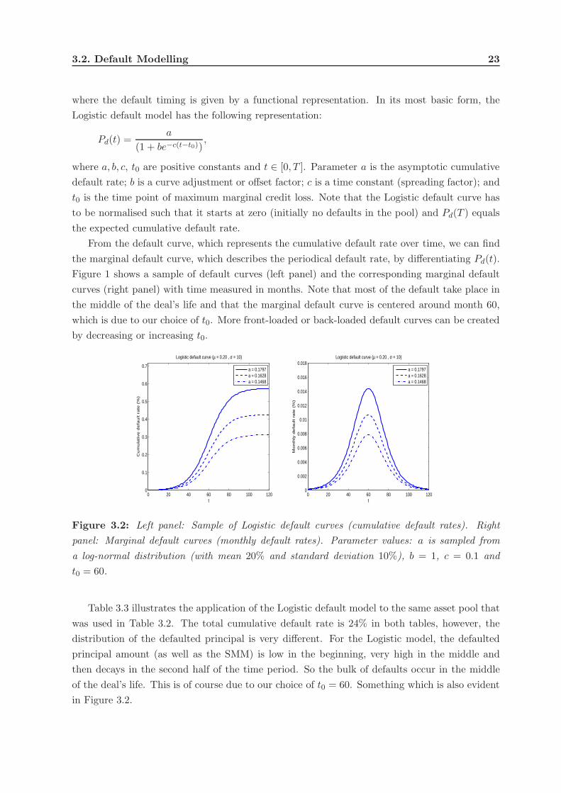
where the default timing is given by a functional representation. In its most basic form, the

Logistic default model has the following representation:

Pd(t) =a

(1 + be−c(t−t0)),

where a, b, c, t0 are positive constants and t ∈ [0, T ]. Parameter a is the asymptotic cumulative

default rate; b is a curve adjustment or offset factor; c is a time constant (spreading factor); and

t0 is the time point of maximum marginal credit loss. Note that the Logistic default curve has

to be normalised such that it starts at zero (initially no defaults in the pool) and Pd(T ) equals

the expected cumulative default rate.

From the default curve, which represents the cumulative default rate over time, we can find

the marginal default curve, which describes the periodical default rate, by differentiating Pd(t).

Figure 1 shows a sample of default curves (left panel) and the corresponding marginal default

curves (right panel) with time measured in months. Note that most of the default take place in

the middle of the deal’s life and that the marginal default curve is centered around month 60,

which is due to our choice of t0. More front-loaded or back-loaded default curves can be created

by decreasing or increasing t0.

0 20 40 60 80 100 1200

0.1

0.2

0.3

0.4

0.5

0.6

0.7

t

Cu

mu

lative

de

fau

lt r

ate

(%

)

Logistic default curve (µ = 0.20 , σ = 10)

a = 0.1797a = 0.1628a = 0.1468

0 20 40 60 80 100 1200

0.002

0.004

0.006

0.008

0.01

0.012

0.014

0.016

0.018

t

Mo

nth

ly d

efa

ult r

ate

(%

)


a = 0.1797a = 0.1628a = 0.1468

Figure 3.2: Left panel: Sample of Logistic default curves (cumulative default rates). Right

panel: Marginal default curves (monthly default rates). Parameter values: a is sampled from

a log-normal distribution (with mean 20% and standard deviation 10%), b = 1, c = 0.1 and

t0 = 60.

Table 3.3 illustrates the application of the Logistic default model to the same asset pool that

was used in Table 3.2. The total cumulative default rate is 24% in both tables, however, the

distribution of the defaulted principal is very different. For the Logistic model, the defaulted

principal amount (as well as the SMM) is low in the beginning, very high in the middle and

then decays in the second half of the time period. So the bulk of defaults occur in the middle

of the deal’s life. This is of course due to our choice of t0 = 60. Something which is also evident

in Figure 3.2.




(%)

1 100,000,000 6,255 0.006255 0.006255

2 99,993,745 6,909 0.006909 0.013164

3 99,986,836 7,631 0.007632 0.020795...

......

......

58 89,795,500 593,540 0.660991 10.204500

59 89,201,960 599,480 0.672048 10.798040

60 88,602,480 602,480 0.679981 11.397520

61 88,000,000 602,480 0.684636 12.000000

62 87,397,520 599,480 0.685923 12.602480...

......

......

119 76,006,255 6,909 0.009089 23.993745

120 76,000,000 6,255 0.008230 24.000000

Table 3.3: Illustration of an application of the Logistic default model. The cumulative default

rate is assumed to be 24% of the initial pool balance. No scheduled principal repayments or

prepayments from the asset pool. Parameter values: a = 0.2406, b = 1, c = 0.1 and t0 = 60.

The model can be extended in several ways. Seasoning could be taken into account in the

model and the asymptotic cumulative default rate (a) can be divided into two factors, one

systemic factor and one idiosyncratic factor (see Raynes and Ruthledge (2003)).

The Logistic default model thus has (at least) four parameters that have to be estimated from

data (see, for example, Raynes and Ruthledge (2003) for a discussion on parameter estimation).

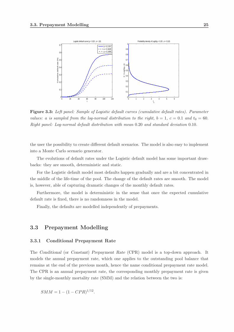
Introducing Randomness

The Logistic default model can easily be used to generate default scenarios. Assuming that we

have a default distribution at hand, for example, the log-normal distribution, describing the

distribution of the cumulative default rate at maturity T . We can then sample an expected

cumulative default rates from the distribution and fit the ’a’ parameter such that Pd(T ) equals

the expected cumulative default rate. Keeping all the other parameters constant. Figure 3.3

shows a sample of Logistic default curves in the left panel, each curve has been generated from

a cumulative default rate sampled from the log-normal distribution shown in the right panel.


The model is attractive because the default curve has an explicit analytic expression. With the

four parameters (a, b, c, t0) many different transformations of the basic shape is possible, giving

3.3. Prepayment Modelling 25

0 20 40 60 80 100 1200

0.1

0.2

0.3

0.4

0.5

0.6

0.7

t

Cu

mu

lative

de

fau

lt r

ate

(%

)


a = 0.1797a = 0.1628a = 0.1468

0 1 2 3 4 5 60

0.1

0.2

0.3

0.4

0.5

0.6

0.7

0.8

0.9

1

X ∼

Lo

gN

(µ, σ

)

fX

Probability density of LogN(µ = 0.20 , σ = 0.10)

Figure 3.3: Left panel: Sample of Logistic default curves (cumulative default rates). Parameter

values: a is sampled from the log-normal distribution to the right, b = 1, c = 0.1 and t0 = 60.

Right panel: Log-normal default distribution with mean 0.20 and standard deviation 0.10.

the user the possibility to create different default scenarios. The model is also easy to implement

into a Monte Carlo scenario generator.

The evolutions of default rates under the Logistic default model has some important draw-

backs: they are smooth, deterministic and static.

For the Logistic default model most defaults happen gradually and are a bit concentrated in

the middle of the life-time of the pool. The change of the default rates are smooth. The model

is, however, able of capturing dramatic changes of the monthly default rates.

Furthermore, the model is deterministic in the sense that once the expected cumulative

default rate is fixed, there is no randomness in the model.

Finally, the defaults are modelled independently of prepayments.

3.3 Prepayment Modelling

3.3.1 Conditional Prepayment Rate

The Conditional (or Constant) Prepayment Rate (CPR) model is a top-down approach. It

models the annual prepayment rate, which one applies to the outstanding pool balance that

remains at the end of the previous month, hence the name conditional prepayment rate model.

The CPR is an annual prepayment rate, the corresponding monthly prepayment rate is given

by the single-monthly mortality rate (SMM) and the relation between the two is:

SMM = 1 − (1 − CPR)1/12.



The strength of the CPR model lies in it simplicity. It allows the user to easily introduce stresses

on the prepayment rate.

A drawback of the CPR model is that the prepayment rate is constant over the life of the

deal, implying that the prepayments as measured in euro amounts are largest in the beginning of

the deal’s life and then decreases. A more reasonable assumption about the prepayment behavior

of loans would be that prepayments ramp-up over an initial period, such that the prepayments

are larger after the loans have seasoned.1

3.3.2 The PSA Benchmark

The Public Securities Association (PSA) benchmark for 30-year mortgages2 is a model which

tries to model the seasoning behaviour of prepayments by including a ramp-up over an initial

period. It models a monthly series of annual prepayment rates: starting with a CPR of 0.2% for

the first month after origination of the loans followed by a monthly increase of the CPR by an

additional 0.2% per annum for the next 30 months when it reaches 6% per year, and after that

staying fixed at a 6% CPR for the remaining years. That is, the marginal prepayment curve

(monthly fraction of prepayments) is of the form:

CPR(t) =

6%30 t , 0 ≤ t ≤ 30

6% , 30 < t ≤ 360,

t=1,2,...,360 months. Remember that this is annual prepayment rates. The single-monthly

prepayment rates are

SMM(t) = 1 − (1 − CPR(t))1/12.

Speed-up or slow-down of the PSA benchmark is possible:

• 50 PSA means one-half the CPR of the PSA benchmark prepayment rate;

• 200 PSA means two times the CPR of the PSA benchmark prepayment rate.


The possibility to speed-up or slow-down the prepayment speed is giving the model some flexi-

bility.

The PSA benchmark is a deterministic model, with no randomness in the prepayment curve’s

behaviour. And it assumes that the prepayment rate is changing smoothly over time, it is

impossible to model dramatic changes in the prepayment rate of a short time interval, that is,

1 Discussed in Fabozzi and Kothari (2008) page 33.2 The benchmark has been extended to other asset classes such as home equity loans and manufacturing housing,

with adjustments to fit the stylized features of those assets, Fabozzi and Kothari (2008).


to introduce the possibility that the prepayment rate suddenly jumps. Finally, under the PSA

benchmark the ramp-up of prepayments always takes place during the first 30 months and the

rate is after that constant.

3.3.3 A Generalised CPR Model

A generalisation of the PSA benchmark is to model the monthly prepayment rates with the

same functional form as the CPR above. That is, instead of assuming that CPR(t) has the

functional form above, we assume now that SMM(t) can be described like that. The marginal

prepayment curve (monthly fraction of prepayments) is described as follows:

pp(t) =

apt , 0 ≤ t ≤ t0p

apt0p , t0p < t ≤ T,

where ap is the single-monthly prepayment rate increase.

The prepayment curve, i.e., the cumulative prepayment rate, is found by calculating the area

under the marginal prepayment curve:

Pp(t) =

ap

2 t2 , 0 ≤ t ≤ t0p

ap

2 t20p + apt0p(t − t0p) , t0p < t ≤ T

The model has two parameters:

• t0p: the time where one switches to a constant CPR (t0p = 30 months in PSA);

• Pp(T ): the cumulative prepayment rate at maturity. For example, Pp(T ) = 0.20 means

that 20% of the initial portfolio have prepaid at maturity T . Can be sampled from a

prepayment distribution.

Once the parameters are set, one can calculate the rate increase per month

ap =Pp(T )

t20p

2 + t0p(T − t0p).

Introducing Randomness

The generation of prepayment scenarios can easily be done with the generalised prepayment

model introduced above. Assuming that we have a prepayment distribution at hand, for example,

the log-normal distribution, describing the distribution of the cumulative prepayment rate at

maturity T . We can then sample an expected cumulative prepayment rate from the distribution,

and fit the ap parameter such that Pp(T ) equals the expected cumulative prepayment rate.

Figure 3.4 shows a sample of marginal prepayment curves and the corresponding cumulative

prepayment curves.


0 20 40 60 80 100 1200

0.5

1

1.5

2

2.5

3x 10

−3

t

pp(t

)

Marginal prepayment curve

ap = 0.000048

ap = 0.000043

ap = 0.000029

ap = 0.000022

ap = 0.000021

0 20 40 60 80 100 1200

0.05

0.1

0.15

0.2

0.25

0.3

0.35

t

Pp(t

)

Cumulative prepayment curve

ap = 0.000048

ap = 0.000043

ap = 0.000029

ap = 0.000022

ap = 0.000021

Figure 3.4: Left panel: Sample of marginal prepayment curves (monthly fraction of prepay-

ments) of the generalised CPR model. Right panel: The corresponding cumulative prepayment

curves of the generalised CPR model. The prepayment distribution is assumed to be log-normal.

The mean and standard deviation of the empirical prepayment distribution is µp = 0.20 and

σp = 0.10.


The evolution of prepayment rates under the generalised CPR model is smooth and deterministic.

The prepayment curve is smooth, no jumps are present, and it is completely determined once

t0p and Pp(T ) are chosen. Furthermore, after t0p the model assumes that the prepayment rate

is constant.

Chapter 4

Stochastic Models

4.1 Introduction

As was discussed in the previous chapter the traditional default and prepayment models has

limited possibilities to capture the stochastic nature of the phenomena they are set to model.

In the present chapter we propose a number of models that incorporate the stylized features of

defaults and prepayments.

By modelling the evolution of defaults and prepayments with stochastic processes we can

achieve three objectives:

• Stochastic timing of defaults and prepayments.

• Stochastic monthly default and prepayment rates.

• Correlation: between defaults; between prepayments; and between defaults and prepay-

ments.

The models we present here can be divided into:

• Portfolio level models (top-down): Levy Portfolio Models.

• Loan level models (bottom-up): One-factor models (Gaussian and Generic Levy).

The family of stochastic processes know as Levy processes is a powerful tool that has been

used in financial modelling for quite some time now. In the recent years Levy processes have

been applied in the field of credit risk modelling and credit derivatives pricing, see Schoutens

and Cariboni (2009).

29

30 Chapter 4 - Stochastic Models

4.2 Default Modelling

4.2.1 Levy Portfolio Default Model

The Levy portfolio default model models the cumulative default rate on portfolio level. The

default curve, i.e., the fraction of loans that have defaulted at time t, is given by:

Pd(t) = 1 − exp(−Xt),

where X = {Xt, t ≥ 0} is a stochastic process. Because we are modelling the cumulative default

rate the default curve Pd(t) must be non-decreasing over time (since we assume that a defaulted

asset is not becoming cured). To achieve this we need to assume that X = {Xt, t ≥ 0} is

non-decreasing over time, since then exp(−Xt) is non-decreasing. Furthermore, assuming that

all assets in the pool are current (Pd(0) = 0) at the time of issue (t = 0) we need X0 = 0.

Our choice of process comes from the family of stochastic processes called Levy process, more

precisely the single-sided Levy processes. A single-sided Levy process is non-decreasing and the

increments are through jumps.

By using a stochastic process to “drive” the default curve, Pd(t) becomes a random variable,

for all t > 0. In order to generate a default curve scenario, we must first draw a realization of

the process X = {Xt, t ≥ 0}. Moreover, Pd(0) = 0, since we start the Levy process at zero:

X0 = 0.

Example: Gamma Portfolio Default Model

As an example, let us consider a default curve based on a Gamma process G = {Gt, t ≥ 0} with

shape parameter a and scale parameter b. The increment from time 0 to time t of the Gamma

process, i.e., Gt − G0 = Gt (recall that G0 = 0) is a Gamma random variable with distribution

Gamma (at, b), for any t > 0. Consequently, the cumulative default rate at maturity follows the

law 1 − e−GT , where GT ∼ Gamma (aT, b). Using this result, the parameters a and b can be

found by matching the expected value and the variance of the cumulative default rate under

the model to the mean and variance of the default distribution, that is, as the solution to the

following system of equations:

E[

1 − e−GT]

= µd;

Var(

1 − e−GT)

= σ2d,

(4.1)

for predetermined values of the mean µd and standard deviation σd of the default distribution.

Explicit expressions for the left hand sides of (4.1) can be found, by noting that the expected

value and the variance can be written in terms of the characteristic function of the Gamma

distribution.

A sample of Gamma portfolio default curves are shown in Figure 4.1 together with the

corresponding default distribution. The mean and standard deviation of the default distribution

is µd = 0.20 and σd = 0.10, respectively, which implies that XT ∼ Gamma(aT = 2.99, b =


12.90). Note that the realisations of the Gamma default curve shown are very different. There

is one path that very early has a large jump in the cumulative default rate (above 10% in month

2) and then evolves with a few smaller jumps and ends at about 25% in month 120. In contrast

to this path we have a realisation that stays almost at zero until month 59 before jumping to

just below 10% and then at month 100 makes a very large jump to around 30%. What is obvious

from Figure 4.1 is that the Gamma portfolio default model gives a wide spectrum of default

scenarios, from front-loaded default curves to back-loaded.

0 20 40 60 80 100 1200

0.1

0.2

0.3

0.4

0.5

t

Pd(t

)

Gamma portfolio default curve (µ = 0.20 , σ = 0.10)

0 1 2 3 4 50

0.1

0.2

0.3

0.4

0.5

X ∼

1−

e−

GT

fX

Probability density of 1−e−GT

Figure 4.1: Left panel: Sample of Levy portfolio default curves. Right panel: corresponding

default distribution. The mean and standard deviation of the empirical default distribution is

µd = 0.20 and σd = 0.10, respectively, which implies that XT ∼ Gamma(aT = 2.99, b = 12.90).

Note that the default distribution shown in Figure 4.1 is generated by the model. In contrast,

the default distribution in Figure 3.3 is an assumption used to generate default curves, in this

case a log-normal distribution.


The Levy portfolio model is a stochastic portfolio-level approach to model the cumulative default

rate. The model gives a wide range of default scenarios, from front-loaded default curves, where

a majority of defaults takes place early, to back-loaded. The default curves are jump driven,

increasing with random jump sizes.

4.2.2 Normal One-Factor Model

The Normal one-factor model (Vasicek (1987) and Li (1995)) models individual loan be-

haviors and introduce correlation between loans. The model is also used in pricing CDOs and

other portfolio credit derivatives and is also called the Gaussian copula model. The link be-

tween the Normal one-factor model and the Gaussian copula was made by Li (2000). There is a

link between the Normal one-factor model and the structural default model by Merton (1974),


which assumes that an obligor defaulted by the maturity of its obligations if the value of the

obligor’s assets is below the value of its debt. In the Normal one-factor model we model the

creditworthiness of an obligor through the use of a latent variable and records a default if the

latent variable is below a barrier. The latent variable of an obligor is modelled as:

Zn =√

ρX +√

1 − ρXn, n = 1, 2, . . . , N, (4.2)

where X is the systemic factor and Xn, n = 1, 2, . . . , N are the idiosyncratic factors, all are

standard normal random variables (mean 0, standard deviation 1), and ρ is the correlation

between two assets:

Corr(Zm, Zn) = ρ, m 6= n.

The nth loan defaulted by time t if

Zn ≤ Kdn(t),

where Kdn(t) is a preset, time dependent default barrier.

If we assume that the pool consist of large number of homogeneous assets, we can use the

representative line approach and model each individual asset as the “average” of the assets in the

pool. By doing this, we only need to calculate one default barrier Kd(t) and Kdn(t) = Kd(t) for

all n. The default barrier can be chosen such that the default time is exponentially distributed:

P(

Zn ≤ Kd(t))

= ΦZn

(

Kd(t))

= P (τ < t) = 1 − e−λt,

where ΦZn(·) is the standard Normal cumulative distribution function. The λ parameter is set

such that P(

Zn ≤ Kd(T ))

= µd, where µd is the predetermined value for the mean of the default

distribution. Note that Kd(t) is non-decreasing in t, which implies that a defaulted loan stays

defaulted and cannot be cured.

The correlation parameter ρ is set such that the standard deviation of the model match the

standard deviation of the default distribution at time T , σd.

Given a sample Z = (Z1, Z2, ..., ZN ) of (correlated) standard Normal random variables, the

default curve is then given by

Pd(t;Z) =♯{

Zn ≤ Kd(t);n = 1, 2, ..., N}

N, t ≥ 0. (4.3)

In order to simulate default curves, one must thus first generate a sample of standard Normal

random variables Zn satisfying (4.2), and then, at each (discrete) time t, count the number of

Zi’s that are less than or equal to the value of the default barrier Kd(t) at that time.

The left panel of Figure 4.2 shows five default curves, generated by the Normal one-factor

model (4.2) with ρ ≈ 0.121353, such that the mean and standard deviation of the default

distribution are 0.20 and 0.10. We have assumed in this realisation that all assets have the

same default barrier. All curves start at zero and are fully stochastic, but unlike the Levy

portfolio model the Normal one-factor default model does not include any jump dynamics. The

corresponding default distribution is again shown in the right panel.


0 20 40 60 80 100 1200

0.1

0.2

0.3

0.4

0.5

t

Pd(t

)

Normal one−factor default curve (µ = 0.20 , σ = 0.10)

0 1 2 3 4 50

0.1

0.2

0.3

0.4

0.5

#{Z

i ≤ H

T}

f#{Z

i ≤ H

T}

Probability density of the cumulative default rate at time T (ρ = 0.12135)

Figure 4.2: Left panel: Sample of Normal one-factor default curves. Right panel: corresponding


µd = 0.20 and σd = 0.10.

Just as for the Levy portfolio default model we would like to point out that the default

distribution is generated by the model, in contrast to the Logistic model. In Figure 4.2, an

example of a default distribution is shown.

Examples of portfolio default rate (PDR) histograms for different default rate and correlation

assumptions are given in Figure 4.3. As can be seen from the plots, changing the correlation

assumption from 10% to 20%, keeping the default rate fixed will shift the mass of the distribution

towards the lower end of the portfolio default rate range. However, at the same time the

probability to have high PDRs increases. From the four plots in Figure 4.3 it is also possible to

see the change of the PDR distribution when the correlation is kept fixed and the mean default

rate assumption is changed.


The Normal one-factor model is a loan-level approach to modelling the cumulative portfolio

default rate. In the loan-level approach one has the freedom to choose between assuming a

homogeneous or a heterogeneous portfolio. For a large portfolio with quite homogeneous assets

the representative line approach can be used, assuming that each of the assets in the portfolio

behaves as the average asset. For a small heterogeneous portfolio it might be better to model

the assets on an individual basis.

The Normal one-factor model can be used to model both the default and prepayment of an

obligor, which will be evident in the section on prepayment modelling.

A known problem with the Normal one-factor model is that many joint defaults are very

unlikely. The underlying reason is the too light tail-behavior of the standard normal distribution

(a large number of joint defaults will be caused by a very large negative common factor X).


0 10 20 30 40 50 60 70 80 90 1000

0.5

1

1.5

2

2.5

3

3.5

4

4.5

5

Default Rates (% initial portfolio balance defaulted)

Fre

qu

en

cy (

%)

Normal one−factor model: ρ=10%; default mean:20%.

0 10 20 30 40 50 60 70 80 90 1000

0.5

1

1.5

2

2.5

3

3.5

4

4.5

5


Fre

qu

en

cy (

%)


0 10 20 30 40 50 60 70 80 90 1000

0.5

1

1.5

2

2.5

3

3.5

4


Fre

qu

en

cy (

%)


0 10 20 30 40 50 60 70 80 90 1000

0.5

1

1.5

2

2.5

3

3.5

4

4.5

5


Fre

qu

en

cy (

%)


Figure 4.3: Portfolio default rate (gross loss divided by initial outstanding pool balance) dis-

tributions versus correlation and default rate estimated by Monte Carlo simulations of a pool of

2, 000 loans using the Normal one-factor model. No prepayments. Bullet amortisation.

Large Homogeneous Portfolio Approximation

The portfolio default rate (PDR) distribution can be found explicitly for the Normal one-factor

model by assuming that the portfolio is homogeneous, which we already do, and consists of a

large number of assets. Under these assumptions the distribution is given by

FPDR(y) = P (PDR < y) = Φ

(√1 − ρΦ−1(y) − Kd(T )√

ρ

)

, 0 ≤ y ≤ 1, (4.4)

where Kd(T ) = Φ−1(p(T )).

The derivation of the distribution in (4.4) is described in Appendix A.

4.2.3 Generic One-Factor Levy Model

To introduce heavier tails one can use Generic one-factor Levy models (Albrecher et al

(2006)) in which the latent variable of obligor i is of the form

Zn = Yρ + Y(n)1−ρ, n = 1, 2, . . . , N, (4.5)

where Yt and Y(n)t are Levy processes with the same underlying distribution L with distribution

function H1(x). Each Zn has by stationary and independent increment property the same

distribution L. If E[Y 21 ] < ∞, the correlation is again given by:



As for the Normal one-factor model, we again say that a borrower defaults at time t, if Zn

hits a predetermined barrier Kd(t) at that time, where Kd(t) satisfies

P(

Zn ≤ Kd(t))

= 1 − e−λt, (4.6)

with λ determined as in the Normal one-factor model.

As an example we use the Shifted-Gamma model where Y, Yn, n = 1, 2, . . . , N are indepen-

dent and identically distributed shifted Gamma processes

Y = {Yt = tµ − Gt : t ≥ 0},

where µ is a positive constant and Gt is a Gamma process with parameters a and b. Thus, the

latent variable of obligor n is of the form:

Zn = Yρ + Y(n)1−ρ = µ − (Gρ + G

(n)1−ρ), n = 1, 2, . . . , N. (4.7)

In order to simulate default curves, we first have to generate a sample of random variables

Z = (Z1, Z2, ..., ZN ) satisfying (4.5) and then, at each (discrete) time t, count the number of

Zi’s that are less than or equal to the value of the default barrier Kd(t) at that time. Hence,

the default curve is given by

Pd(t;Z) =♯{

Zn ≤ Kd(t);n = 1, 2, ..., N}

N, t ≥ 0. (4.8)

The left panel of Figure 4.4 shows five default curves, generated by the Gamma one-factor

model (4.7) with (µ, a, b) = (1, 1, 1), and ρ ≈ 0.095408, such that the mean and standard

deviation of the default distribution are 0.20 and 0.10. Again, all curves start at zero and are

fully stochastic. The corresponding default distribution is shown in the right panel. Compared

to the previous three default models, the default distribution generated by the Gamma one-

factor model seems to be squeezed around µd and has a significantly larger kurtosis. Again we

do not have to assume a given default distribution, the default distribution will be generated by

the model.

It should also be mentioned that the latter default distribution has a rather heavy right tail

(not shown in the graph), with a substantial probability mass at the 100 % default rate. This

can be explained by looking at the right-hand side of equation (4.7). Since both terms between

brackets are strictly positive and hence cannot compensate each other (unlike the Normal one-

factor model), Zi is bounded from above by µ. Hence, starting with a large systematic risk

factor Y , things can only get worse, i.e. the term between the parentheses can only increase

and therefore Zi can only decrease, when adding the idiosyncratic risk factor Yi. This implies

that when we have a substantially large common factor, it is more likely that all borrowers will

default, than with the Normal one-factor model.


0 20 40 60 80 100 1200

0.05

0.1

0.15

0.2

0.25

t

Pd(t

)

Gamma 1−factor default curve (µ = 0.20 , σ = 0.10)

0 5 10 15 20 25 30 35 400

0.05

0.1

0.15

0.2

0.25

#{Z

i ≤ H

T}

f#{Z

i ≤ H

T}

Probability density of the cumulative default rate at time T (ρ = 0.09541)

Figure 4.4: Left panel: Sample of Gamma one-factor default curves. Right panel: corresponding


µd = 0.20 and σd = 0.10.


The generic Levy one-factor model is a loan-level model, just as the Normal one-factor model,

but with the freedom to choose the underlying probability distribution from a large set of

distributions. The distributions are more heavy tailed than the normal distribution, that is,

give a higher probability to large positive or negative values. A higher probability that the

common factor is a large negative number gives higher probability to have many defaults.

Large Homogeneous Portfolio Approximation

One can find the approximation of the portfolio default rate distribution for large homogeneous

portfolios also under the generic one-factor Levy models, see Albrecher et al (2006).

4.3 Prepayment Modelling

4.3.1 Levy Portfolio Prepayment Model

The Levy portfolio prepayment model is completely analogous to the Levy portfolio default

model described in Section 4.2.1.

4.3.2 Normal One-Factor Prepayment Model

The Normal one-factor prepayment model starts from the same underlying philosophy as its

default equivalent. The idea is to model prepayment as an event that occurs if the credit

worthiness of the obligor is above a certain level, the so called prepayment barrier, just as

default was assumed to occur if the credit worthiness of the obligor was below a barrier, the so

called default barrier.


The asset’s latent variable is modelled by:

Zn =√

ρX +√

1 − ρXn, n = 1, 2, . . . , N, (4.9)

where X is the systemic factor and Xn, n = 1, 2, . . . , N are the idiosyncratic factors, all are

standard normal random variables (mean 0, standard deviation 1), and ρ is the correlation

between two assets: Corr(Zm, Zn) = ρ, m 6= n.

The prepayment barrier Kpn(t) is chosen such that the probability of prepayment before time

t equals Pp(t) in the generalised CPR model:

P (Zn ≥ Kpn(t)) = 1 − ΦZn (Kp

n(t)) = Pp(t).

Thus, Kpn(t) = Φ−1(1−Pp(t)), where Φ−1 denotes the inverse of the standard Normal distribution

function. Note that Kpn(t) is non-increasing in t, which implies that a prepaid loan does not

reappear in the pool and, thus, that the prepayment curve is non-decreasing.

0 10 20 30 40 50 60 70 80 90 100−6

−4

−2

0

2

4

6

t

Prepayment

Default

Loan 1

Loan 2

Loan 3

Prepayment barrier

Default barrier

Figure 4.5: Example of a default barrier and a prepayment barrier in a one-factor model.

Figure 4.5 shows how a prepayment barrier and a default barrier can be combined in an

one-factor model.

The prepayment curve is defined as:

Pp(t;Z) =♯ {Zn ≥ Kp(t);n = 1, 2, ..., N}

N, t ≥ 0. (4.10)

Comparing the prepayment curves in Figure 4.6 with the curves generated by the generalised

CPR model in the right panel of Figure 3.4, one can see that they are similar in shape due to

the fact that the prepayment barrier is chosen such that the probability of prepayment of an

individual obligor equals the cumulative prepayment rate given by the generalised CPR model.

However, the prepayment curves generated by the Normal one-factor model are stochastic as

can be seen from the non-linear behaviour of the curves.

Note that the prepayment distribution is generated by the model. This is in contrast with the

prepayment distribution shown for the generalised CPR model in Figure 3.4 where we assumed

the log-normal distribution.


0 20 40 60 80 100 1200

0.1

0.2

0.3

0.4

0.5

t

Pp(t

)

Normal 1−factor prepayment curve (µ = 0.20 , σ = 0.10)

0 0.5 1 1.5 2 2.5 3 3.5 4 4.50

0.1

0.2

0.3

0.4

0.5

#{Z

i ≥ H

T}

f#{Z

i ≥ H

T}

Probability density of the cumulative prepayment rate at time T (ρ = 0.12135)

Figure 4.6: Left panel: Sample of Normal one-factor prepayment curves. Right panel: Corre-

sponding prepayment distribution. The mean and standard deviation of the empirical prepayment

distribution is µp = 0.20 and σp = 0.10.


The evolution of the prepayment curve is stochastic, not deterministic. Furthermore, with the

Normal one-factor model it is possible to model both default and prepayment of a single obligor

at the same time.

See also comments on the Normal one-factor default model.

Chapter 5

Rating Agencies Methodologies

5.1 Introduction

To derive ratings of the asset backed securities (ABSs) in a securitisation structure the rating

agencies assesses the risks in the deal and how well the structure mitigates these risks. The

assessment is a combination of qualitative analysis and quantitative methodologies.

The present chapter gives an overview of two of the major rating agencies, Moody’s and

Standard & Poor’s, quantitative methodologies to provide ratings to ABSs, in particular to

ABSs backed by SME loans.

5.2 Moody’s

In this section we focus on Moody’s approach to rating SME transactions, although the basic

methodologies is similar for other asset classes. As was already mentioned in Chapter 2, Moody’s

rating is an expected loss assessment, which incorporate the assessment of both the likelihood of

default and the severity of loss, given default. The quantitative rating is based on the results from

a quantitative model, which calculates the Expected Loss and the Expected Weighted Average

Life of an ABS note. This quantitative rating is combined with a qualitative analysis, which

includes an operational overview of the originator and the servicer and legal issues (transfer of

assets and bankruptcy), to derive a final rating (Moody’s (2001) and Moody’s (2007b)).

The quantitative rating methodology used depends on the size and granularity of the un-

derlying SME portfolio. For small or non-granular portfolios, such as CDO’s, Moody’s takes a

bottom-up approach and use factor models (typically based on the Gaussian-copula approach,

for example the Normal one-factor model presented previously) for the analysis. For granular

portfolios Moody’s adopt a default distribution (Lognormal or Normal Inverse) approach, to

model the cumulative default rate at the deal maturity. The factor models are implemented in

Moody’s CDOROMTM and Moody’s STARFINDERTM (see Moody’s (2006b)); the granular

approach in Moody’s ABSROMTM (see Moody’s (2006a)).

In general, Moody’s classifies SME portfolios with more than 1, 000 assets and no major

39

40 Chapter 5 - Rating Agencies Methodologies

concentrations as ABS SME.1

General information guidelines describing the data that Moody’s would like to receive from

the originator for SME securitisation transactions are given in Moody’s (2007b).

5.2.1 Non-Granular Portfolios

For concentrated, heterogeneous pools the main tool for deriving a default distribution is

Moody’s CDOROMTM . The portfolio default distribution will be directly derived from Monte

Carlo simulations, which simulates the default of each individual asset based on a factor model

as described previously in Section 4.2.2. The factor models used are typically based on one

factor:

Zn =√

ρcXc +√

1 − ρcXn,

or, on two factors:

Zn =√

ρcXc +√

ρiXi +√

1 − ρc − ρiXn,

where Xc is the common global factor, Xi is an industry factor, Xn, n = 1, 2, . . . , N is the

individual firm specific factor, and ρc and ρi is the global inter-industry and the sector specific

intra-industry correlation assumptions, respectively, see Moody’s (2007a).

The input parameters in the model are the probability of default of each individual asset

and the asset correlation. The individual default probability is typically derived from either (i)

public ratings, (ii) credit estimates or (iii) a mapping between the originator’s internal rating

system and Moody’s rating scale. The correlation is derived from Moody’s corporate correlation

framework adopted in global CDOs. However, Moody’s stresses the correlation parameters from

3% to 6% depending on the specific characteristics of the portfolio, to account for a higher

geographical concentration and industrial clustering typically present in SME pools.2

In contrast to the approach for granular portfolios described below, the default timing is

directly generated in the factor models since the default of each individual asset is simulated.

In CDOROMTM the recovery rates are stochastic and assumed to be distributed according

to a Beta distribution applied to each defaulted asset.3

To derive a rating, the present value of the loss for the note and the note’s weighted average

life are calculated for each simulation run and the averages over all simulations are taken as esti-

mates of the expected loss and the expected weighted average life. (A more detailed description

is given in the section on granular portfolios.)

The rating of the note is found from Moody’s Idealised Cumulative Expected Loss Table,

which map the Expected Average Life and Expected Loss combination to a specific quantitative

rating. An example of such a table is given in Moody’s (2000b).

1 To discriminate non-granular, granular and intermediate portfolios, Moody’s calculates the Effective Number

of Obligors, based on the Herfindahl index (see Moody’s (2007d).2 Moody’s (2007d), p. 4.3 Moody’s (2007d), p. 8.

5.2. Moody’s 41

5.2.2 Granular Portfolios

For granular portfolios a default distribution for the total cumulative default rate (expressed as

per cent of initial portfolio outstanding principal amount) over the life of the pool is assumed,

typically a Normal Inverse4 distribution (previously Moody’s used the Lognormal distribution

as standard, but this has changed (Moody’s (2007d))). The default distribution is characterised

by two parameters: the mean and the standard deviation, that has to be estimated. Moody’s

estimates these parameters from historical static cohort data provided by the originator. This

data is typically given in a Static cumulative default rate table describing different cohorts

(or vintages) of pools of loans and the cumulative default rate over a number of periods after

origination. From this data estimates of the mean and standard deviation is derived. The basic

methodology of how to extrapolate, clean and adjust for seasoning is described in Moody’s

(2005b). The parameter estimation based on historical cohort data is (almost) only applicable

at the time the transaction is issued, because it is rarely that updated cohort data is made

available at a later stage after the closing date. To handle this problem Moody’s has developed

a methodology to revise the default assumptions over the life of an ABS transaction (Moody’s

(2008)). The method takes as input transaction specific performance data, such as delinquency

rates, historical periodic default or loss rates and historical portfolio redemption rates.

Based on the default distribution a set of Default Scenarios are derived and the scenario

probability is given by the default distribution. The default scenarios are 0.00%, 0.10%, 0.20%, . . .

and the scenario probability is the probability that the default rate falls between two consecutive

default scenarios.5 The Normal Inverse distribution and the 20% default scenario with its

associated probability are illustrated in Figure 5.1.

To distribute the defaults over the life of the pool a Default Timing vector is defined. For

each period, the corresponding element in the Default Timing vector is the percentage of the

total cumulative default rate that will be applicable in that period. The Default Timing vector

is used to calculate the outstanding amount of the defaulted loans per period in each default

scenario:

Defaulted Amount(period i, scenario s) = DefaultTiming (period i)

×DefaultRate(scenario s)

×Original PortfolioAmount.

The default timing is preferably derived from historical static cohort data on defaults (Moody’s

(2007d)).

For granular portfolios the recovery rate is assumed to be stochastic with a Normal distri-

4 The Normal Inverse distribution is an approximation of the default distribution if the Normal one-factor model

is used for a large homogeneous portfolio, see Appendix A and Moody’s (2003) and Moody’s (2007a).5 Moody’s (2006a), p. 34.


0 20 40 60 80 1000

0.05

0.1

0.15

0.2

0.25

0.3

0.35

0.4


Pro

babi

lity

(%)

Probability of 20% default rate

Figure 5.1: Illustration of a Normal Inverse default distribution. The 20% Default Scenario

and its associated probability is marked with a bar. The asset correlation was assumed to be

ρ = 20%, and the mean cumulative default rate 20%. The default barrier was estimated as

described in the section on the Normal one-factor default model.

bution and is applied on a portfolio basis.6 Historical recovery data provided by the originator

is used in order to determine the recovery rate. In ABSROMTM a Recovery Timing vector is

used to specify the timing of the recoveries.

For the prepayments Moody’s assumes a fixed annual constant prepayment rate (CPR),

which is estimated from the originator’s historical data.

To come to a rating Moody′s ABSROMTM calculates the Expected Average Life (or weighted

average life) and the Expected Loss of the note (see Moody’s (2006a), p. 32-33). The Expected

Average Life of the note is given by:

Last Default Scenario∑

s=1st Default Scenario

Weighted Average Life(scenario s) × Probability(scenario s),

where Weighted Average Life(scenario s) is:

Legal Maturity Date∑

i=1st Period

Outstanding Note Amount(Period i, scenario s)

Original Note Amount × Number of Periods per Annum.

The expected loss is calculated as the sum-product of the probability of each default scenario

and the corresponding Relative Net Present Value-Loss. For each default scenario, the Relative

Net Present Value-Loss for a note is calculated by discounting the cashflows (both interest and

6 Moody’s (2007d), p. 8. What is meant with “applied on a portfolio basis” is not clear. Using a Normal

distribution for the recovery rate implies that the recovery rate can become negative. However, Moody’s

argues that by the Law of Large Numbers, if all LGDs are independent and identically distributed, the average

LGD will be almost equal to its expected value for high default rates, which implies that the right tail of

the loss distribution will not depend on the shape of the LGD distribution for each asset. See discussion in

footnotes 30 and 31 in Moody’s (2003), p. 18 and 19, respectively.

5.3. Standard and Poor’s 43

principal) received on that note with a discount rate which is equal to the rate of that note and

by comparing it to the initial outstanding amount on the note (Moody’s (2006a), p. 33):

Relative NPV Loss(Scenario s) =Nominal Initial Amount − NPV Cashflow(Scenario s)

Nominal Initial Amount.

The expected loss is then given by:

Expected Loss =

Last Default Scenario∑

s=1st Default Scenario

RelativeNPV Loss(Scenario s) ·Probability(Scenario s).

For a fixed rate note the discount rate will be the promised coupon rate and for a floating

rate note it will be the realised benchmark rate plus the note’s margin.

The rating of the note is found from Moody’s Idealised Cumulative Expected Loss Table,

which map the Expected Average Life and Expected Loss combination to a specific quantitative

rating. An example of such a table is given in Moody’s (2000b).

V Scores and Parameter Sensitivity

Moody’s has recently introduced two changes to the way structured finance ratings are presented:

V Scores and Parameter Sensitivities. Moody’s V Scores “provide a relative assessment of the

quality of available credit information and the potential variability around various inputs to a

rating determination.”.7 The Parameter Sensitivities “provide a quantitative/model-indicated

calculation of the number of rating notches that a Moody’s-rated structured finance security

may vary if certain input parameters used in the initial rating process differed.”.8

It is intended that the V Scores shall provide a ranking of transactions by the potential of

rating changes due to uncertainty around the assumptions made during the rating process. V

Scores are a qualitative assessment of the potential of rating changes due to, among others,

data quality, historical performance, transaction complexity, and the transaction governance

that underly the ratings.

To analyse the parameter sensitivity, typically, the two key input parameters that have the

greatest impact within the sector will be stressed. For example, the mean portfolio default rate

and the mean recovery rate can be assumed to vary between 12%, 14% and 16% and 30%, 40%

and 50%, respectively. For each stressed scenario (i.e. each combination of default rate and

recovery rate in our example) a new loss distribution is generated under which the notes are

re-assessed.

5.3 Standard and Poor’s

As mentioned before, the meaning of Standard and Poor’s (S&P’s) rating is the assessment of

timely payment of interest and the ultimate payment of principal no later than the legal final

7 Moody’s (2009b), p. 1.8 Moody’s (2009b), p. 1.


maturity date. It is only the credit quality of structure finance securities that is addressed, and

the ratings framework is based on the likelihood of default and not on expected loss or loss given

default (Standard and Poor’s (2007b)).

S&P’s employs a principle-based methodology for rating structured finance securities, out-

lined in Standard and Poor’s (2007b). The core methodologies for analysing and rating se-

curitisation transactions contains five key areas of analysis: credit quality of the securitised

assets; payment structure and cash flow mechanics; legal and regulatory risks; operational and

administrative risks; and counterparty risk. We will focus on the quantitative parts in the rating

process here, namely credit quality of the securitised assets and payment structure and cash flow

mechanics.

5.3.1 Credit Quality of Defaulted Assets

For most ABSs, RMBSs and CDOs backed by pools of loans, receivables or corporate debt

the credit quality analysis focuses on determining under “worst-case” scenarios the portion of

the original asset pool that will default and the portion of these defaulted assets that can be

recovered. From this the potential ultimate loss on the debt issue can be derived (Standard and

Poor’s (2007b), p. 7).

S&P’s has three main SME transaction categories (Standard and Poor’s (2009a), p. 2):

• Granular SME transactions;

• Transactions with lumpy assets or high sector exposure; and

• Hybrid bespoke transactions.

SME transactions with highly granular characteristic with assets spread across different sectors

and industries are categorised as granular transactions. Typically a granular transaction is a

securitisation of a cross-section of a bank’s SME loan portfolio. In the second category, the

portfolio has a skewed risk profile due to an uneven and high exposure to a small number of

obligors or economic sectors. Hybrid bespoke transactions are often created for the purpose of

obtaining repo financing under central bank financing schemes and contains a mix of SME assets

together with large corporate loans and residential and commercial mortgages.

Based on these categories, different analytical approaches and assumptions are applied to

rate transactions backed by SME loans (Standard and Poor’s (2009a), p. 3):

• The actuarial approach;

• Probability of default and stochastic modelling approach; and

• Secured real estate default analysis.

In the actuarial approach, base case portfolio default rates and recovery rates are derived

using historical gross loss rates and recovery data. These default and recovery rates are then used


to stress and simulate defaults and recoveries over time in different rating scenarios. Typically

this approach is applied to granular SME transactions.

The second approach, probability of default and stochastic modelling, is based on S&P’s

CDO Evaluatorr model. The model uses Monte Carlo simulation to assess the credit quality

of an asset portfolio, taking as input the credit rating, notional exposure and maturity of each

asset, as well as the correlation between each pair of assets. The output from the model is a

probability distribution of potential portfolio default rates, which is the base for a set of scenario

default rates (SDRs), one for each rating level. The SDR is the portfolio loss an ABS must be

able to withstand without defaulting. The CDO Evaluatorr is based on the Gaussian copula

model by Li (2000).

The final approach is used for assets that are secured on real estate collateral and is a weighted

average foreclosure frequency (WAFF) and weighted average loss severity (WALS) approach.

To determine the likely default and loss on a loan underlying loan level characteristics, such as,

loan-to-value (LTV) ratio, seasoning and regional concentrations are used.

The above described approaches are carried out together with a detailed cash flow analysis,

which is described below.

CDO Evaluatorr Model

As mentioned above the CDO Evaluatorr model uses Monte Carlo simulations to assess the

credit quality of the asset pool. The output of this assessment is a probability distribution of

potential portfolio default rates. The CDO Evaluatorr model is a bottom-up approach, where

each individual asset is modelled. The modelling is based on the Gaussian copula model proposed

by Li (2000). In fact, the Gaussian copula model is the Normal factor model “translated” into

the language of copula functions. Hence, both Moody’s and S&P’s base their quantitative

modelling of non-granular portfolios on the same mathematical model.

The CDO Evaluatorr allows for both fixed and stochastic (beta distributed) recoveries, it

is however not clear if stochastic recoveries are applicable for SMEs.9

From the probability distribution of default rates scenario default rates (SDRs) are derived.

The SDR for a specific rating level is the largest portfolio default rate such that the probability

of defaults in the portfolio exceeding the SDR is not greater than the probability of default for

the given rating level and time horizon.

For example, assume that we want to find the SDR for the ’AA’ rating level and a time

horizon of 10 years. We lookup the probability of default associated with the ’AA’ rating in a

credit curve table. A credit curve table contains the probability of default for each rating level

for a series of maturities. Let us say that the probability of default for a 10 year ’AA’ rated

tranche is 1.0%. We now have to find the largest portfolio default rate from the default rate

distribution for which the likelihood of exceeding this value is less than or equal to 1.0%. This

9 CDO Evaluatorr Version 4.1 User Guide (version 1.36), Standard & Poor’s Structured Finance Group, De-

cember 2008, p. 91.


is illustrated in Figure 5.2. The SDR equals 34% in this example and the likelihood that the

defaults in the portfolio exceeds 34% is 0.96%.

0 5 10 15 20 25 30 35 40 450

1

2

3

4

5

6

7

Default Rate (% initial portfolio balance defaulted)

Pro

babi

lity

(%)

SDR = 34%

Figure 5.2: Example of a probability distribution of portfolio default rates and the scenario

default rate (34%) associated with a probability of default of 1.0%.

5.3.2 Cash Flow Modelling

The cash flow analysis evaluates the availability of funds for timely payment of interest and

ultimate payment of principal following the conditions of each rated class of notes and is used

to determine the credit support levels for each rated class of notes. The cash flow analysis is

done for each rated class of notes by stressing the cash flow from the asset pool. The severity

of the stress scenarios applied to the cash flow depend on the desired rating. The cash flow

analysis described here is the one used in combination with the CDO Evaluatorr model and is

based on the following reports: Standard and Poor’s (2004b), Standard and Poor’s (2006a),

and Standard and Poor’s (2006b).10

The stress tests are performed with respect to among other things:11

• Default timing;

• Delinquencies (if applicable);

• Recovery rates and timing;

• Interest rate hedging (including interest rate stresses);

10 It is not clear if the cash flow analysis done in combination with the actuarial approach is the same from the

documentation. In Standard and Poor’s (2003) p. 11 a short description is made, but it does not clarify if the

same set of stress scenarios for each rating level is used in combination with the actuarial approach as with the

CDO Evaluatorr model approach.11 Standard and Poor’s (2004b) and Standard and Poor’s (2006a). These reports are only discussing the cash

flow modelling of stressed scenarios in combination with the CDO Evaluatorr model.


• Prepayments (if applicable); and

• Senior fees.

We describe here only the default timing and the recovery timing stresses.

Default Timing Stresses

S&P’s applies four standard default patterns and a few additional default patterns (saw-tooth

patterns and expected case patterns) to stress the cash flow.12 We will here describe the four

standard patterns, given in Table 5.1, and refer the interested reader to Standard and Poor’s

(2004b) for a description of the additional patterns. Each pattern expresses the percentage of

the cumulative default rate that occurs ever year once defaults starts. As can be seen from

Table 5.1, all defaults are assumed to occur during four or five years once defaults starts. The

Annual defaults (% of cumulative defaults)

Year 1 Year 2 Year 3 Year 4 Year 5

Pattern I 15 30 30 15 10

Pattern II 40 20 20 10 10

Pattern III 20 20 20 20 20

Pattern IV 25 25 25 25 -

Table 5.1: Standard & Poor’s standard default patterns. Annual defaults as a percentage

of cumulative defaults. Source: “Update To General Cash Flow Analytics Criteria For CDO

Securitizations”, Standard and Poor’s, October 17, 2006, p. 7.

annual default rates given in Table 5.1 can be distributed evenly across the four quarters of the

year with defaults occurring on the last day of each quarter. This applies to all years except

the first year of the transaction, in which the entire default amount is supposed to occur at the

last day of the year, because S&P’s assumes that some time elapse before defaults occur in a

newly gathered portfolio. An exception to this is the case when the portfolio contains a large

concentration of low credit quality assets.13

It is important to note that the default patterns are applied to the original par balance of the

portfolio. As an example, assume that we apply Pattern I to a cumulative default rate of 20%

and a pool with original balance 100. Then the original pool par balance experience defaults of

3%(= 15% · 20%), 6%, 6%, 3% and 2%, respectively, in the five years the pattern is covering,

or, equivalently, 3, 6, 6, 3 and 2.

12 S&P’s uses this deterministic modelling approach with default patterns for application to cash flow CDO

transactions. For synthetic CDO transactions S&P’s uses the default timing patterns generated by the CDO

Evaluatorr model, see Standard and Poor’s (2006b), p. 7.13 Standard and Poor’s (2004b) p. 10.


These patterns are combined with default timing stresses, which means that the start of a

specific pattern is delayed by a number of years. That is, the cash flow analysis is run for a

specific pattern starting in year 1, and then for the same pattern starting in year 2, and so

on. The starting times of the patterns are delayed to the point where the final default in the

pattern occurs in the same year as the portfolio balance is expected to mature, which depends

on the length of the reinvestment period and the weighted average life of the assets (given by the

weighted average life covenant in the offering circular). These default timing stresses, that is,

the delays, are different for different rating levels.14 An example of the different starting years

for different rating categories is given in Table 5.2.

Reinvestment WAL Tranche

period covenant∗ ’AAA’ ’AA’ ’A’ ’BBB’ ’BB’ ’B’

5 4 1 to 5 1 to 5 1 to 4 1 to 3 1 to 2 1

5 6 1 to 7 1 to 7 1 to 6 1 to 5 1 to 4 1 to 3

Table 5.2: Example of starting years for Standard & Poor’s standard default patterns. *The

WAL covenant at the end of the reinvestment period as stated in the offering circular. Source:

“CDO Spotlight: General Cash Flow Analytics for CDO Securitizations”, Standard and Poor’s,

August 25, 2004, p. 8.

An illustration of how the default scenarios can look like when Pattern I in Table 5.1 is

combined with the default timing stresses given in Table 5.2 for a ’AAA’ or ’AA’ rated tranche

for a transaction with five years reinvestment period and a WAL covenant of four years is shown

in Table 5.3. Note that in the table the annual defaults are shown as a percentage of the total

cumulative defaults.

Annual defaults (% of cumulative defaults)

Scenario Year 1 Year 2 Year 3 Year 4 Year 5 Year 6 Year 7 Year 8 Year 9

1 15 30 30 15 10 0 0 0 0

2 0 15 30 30 15 10 0 0 0

3 0 0 15 30 30 15 10 0 0

4 0 0 0 15 30 30 15 10 0

5 0 0 0 0 15 30 30 15 10

Table 5.3: Example of default scenarios for analysing a ’AAA’ or ’AA’ tranche when the

reinvestment period is 5 years and WAL covenant is a 4 years. Annual defaults as a percentage

of cumulative defaults.

14 S&P’s propose to change this in such a way that default timing stresses for rating level ’A’ through ’B’ are the

same as for ’AAA’ and ’AA’, see Standard and Poor’s (2009b).


Recoveries

Recovery rates are established on a transaction-by-transaction basis taking into account factors

such as: the level of experience of the originator; transaction-specific investment guidelines and

replenishment criteria; workout procedures and timing of expected recoveries; and location of

the defaulted obligor. S&P’s has established recovery ranges per country for each transaction,

partly based on transaction-specific data available.15

Recoveries on defaulted loans are assumed to occur over a three-year workout period, with

the recovery timing as given in Table 5.4. Note that the recoveries are realised in the end of the

period.

U.K. France Germany Rest of Europe

End of year 1 75% - - -

End of year 2 25% 50% 25% 50%

End of year 3 - 50% 75% 50%

Table 5.4: Standard & Poor’s recovery timing assumption as percentage of total recovery rate

assumed in each year during workout period for SME loans. Source: “Credit Risk Tracker

Strengthens Rating Analysis of CLOs of Eurpoean SME Loans”, Standard and Poor’s, June 10,

2004, p. 6.

5.3.3 Achieving a Desired Rating

The stress scenarios used in the cash flow analysis aim to assess if the ABS under consideration

can withstand the stresses associated with the sought rating level and therefore can receive the

corresponding rating level.

For each stress scenario, the output from the cash flow analysis is the break even default rate

(BDR) the portfolio can withstand and still generate adequate cash flow to meet contractual

payments of interest and principal on the class of notes subject to the particular stress scenario.

The break even default rate is found by first finding the minimum credit enhancement level given

by the subordination structure, i.e., the note’s attachment point, such that the note’s overall

credit performance is adequate for the targeted rating level. This minimum credit enhancement

is then translated into a portfolio default rate, which is the so called break even default rate.

Thus, for each rated class of notes, the result of the cash flow analysis is a set of break

even default rates (BDRs), one for each stress scenario. The desired rating of a class of notes

is achieved by comparing the BDRs with the SDR for that rating level. Assume, for example,

that we pick the minimum BDR for each rating level and compare it with the corresponding

SDR. If the SDR for the ’AA’ rating level is 34%, then a tranche can receive a ’AA’ rating if

the corresponding minimum BDR for that tranche is equal to or greater than 34%.

15 Standard and Poor’s (2004a), p. 5.


To pick out the BDR for each rated class that should be compared with the corresponding

SDR, S&P’s uses a percentile approach, which differentiate the application of BDRs across rating

categories.16 The break even percentiles by rating is shown in Table 5.5.

Tranche rating Percentile

AAA 5th

AA 10th

A 35th

BBB 50th

BB 60th

B 70th

Table 5.5: Break even percentiles by rating. Note that for all rating categories ’AA’, ’A’ and

so until ’B’ include rating subcategories, for example, ’AA’ percentile also applies to ’AA+’ and

’AA-’. Source: “Update To General Cash Flow Analytics Criteria For CDO Securitizations”,

Standard and Poor’s, October 17, 2006, p. 3.

In the example above, this would mean that the 10th percentile BDR should be equal to or

greater than 34% if the tranche should receive a ’AA’ rating.

5.4 Conclusions

The interpretation of a rating is different over the various rating agencies. Moody’s rating is an

assessment of the expected loss that a class of notes may experience, while S&P’s rating is an

assessment of the probability of default of the class of notes and addresses the timely payment

of interest and the ultimate payment of principal.

Both Moody’s and S&P’s discriminate between granular and non-granular SME portfolios

and applies different approaches to the two categories.

For non-granular SME portfolios both rating agencies use a loan-by-loan or bottom-up ap-

proach and model each individual asset in the pool. Moody’s uses its CDOROMTM tool, which

uses Normal factor models (with dependence structures based on the Gaussian copula approach);

S&P’s is using its CDO Evaluatorr model, which is based on the Gaussian copula approach. In

both cases, thus, are the underlying mathematical tool to introduce dependence in the portfolios

the Gaussian copula approach. Monte Carlo simulations are used to generate defaults in the

asset pool and to derive a default distribution. The difference between the two methodologies

lies in the use of the tool or model.

In Moody’s methodology, the default scenario generated by each Monte Carlo simulation is

fed into the cash flow model and the losses on the ABSs are derived. This is done for a large

16 Earlier the minimum BDR produced by the cash flow analysis was compared to the scenario default rate (SDR)

for each rating level, see Standard and Poor’s (2006b).

5.4. Conclusions 51

number of simulations and an estimate of the expected loss on each ABS is derived. The cash

flow analysis is thus an integrated part of the simulations. The expected losses are mapped to

a rating for each ABS using Moody’s loss rate tables.

In S&P’s methodology, the Monte Carlo simulations generate a probability distribution of

potential portfolio default rates that is used to derive a set of scenario default rates (SDRs),

one for each rating level. Each SDR represents the maximum portfolio default rate that an

ABS with the desired rating should be able to withstand without default. These SDRs are then

used to create different stressed rating scenarios that are applied in a cash flow analysis, which

assesses if the ABS under consideration can withstand the stresses associated with the targeted

rating level and therefore can receive the corresponding rating level.

For granular SME portfolios, Moody’s uses its ABSROMTM tool, which uses a default rate

distribution to generate default scenarios and the corresponding likelihood of each scenario.

The default rate distribution’s mean and standard deviation is estimated using historical data.

Running a cash flow model with the different default scenarios, stressing the default timing, the

expected loss on the notes are calculated. S&P’s applies its actuarial approach, for granular

SME portfolios, which is based on deriving base case default and recovery rates from historical

data in order to stress defaults over the life of the transaction in different rating scenarios in a

cash flow analysis.

Chapter 6

Model Risk and Parameter

Sensitivity

6.1 Introduction

To derive ratings of ABSs is partly based on quantitative models for modelling defaults and

prepayments generated in the asset pool. This introduces exposure to model and methodology

risk, because there exists a vast amount of quantitative models and approaches to choose be-

tween, each producing different asset behaviour and portfolio loss distributions. The parameter

values which are used as inputs to the quantitative models, such as, mean cumulative default and

prepayment rates, recoveries, default probabilities, and asset correlations, are unknown quan-

tities and are commonly estimated from historical data or based on subjective assumptions.

This introduce parameter uncertainty into the assessment and it therefore becomes important

to understand the ratings parameter sensitivity.

We observe in the present chapter the important impact the choices of model and parameter

values have on ABS ratings by applying some of the default and prepayment models presented

in Chapter 3 and 4 to a structure with two classes of notes backed by a pool of loans.

This chapter is mainly based on Jonsson et al (2009) and Jonsson and Schoutens (2010).

6.2 The ABS structure

Assets

The asset pool consists of 2,000 level-pay loans that pays principal and interest monthly. The

interest rate is fixed. The pool is static, new loans are not added to the pool. The asset

characteristics are shown in Table 6.1.

53

54 Chapter 6 - Model risk and parameter sensitivity

ASSETS

Initial balance of the asset pool V0 $30,000,000

Number of loans in the asset pool N0 2,000

Weighted Average Maturity of the assets WAM 10 years

Weighted Average Coupon of the assets WAC 12% p.a.

Payment frequency monthly

Reserve target rT 5% (CB∗)

Eligible reinvestment rate 3.92% p.a.

Loss-Given-Default LGD 50%

Lag 5 months

Table 6.1: Asset characteristics. * CB: Current Balance.

Liabilities

This pool of assets backs two classes of notes: A (senior) and B (junior); both having fixed

coupons. The notes are amortized pro-rata during the life of the deal. A reserve fund is used as

an additional credit enhancement. The reserve fund target is 5% of outstanding balance of the

pool. The characteristics of the notes are shown in Table 6.2.

LIABILITIES

Initial balance of the senior note A0 $24,000,000

Premium of the senior note rA 7% p.a.

Initial balance of the subordinated note B0 $6,000,000

Premium of the subordinated note rB 9% p.a.

Servicing fee rsf 1% p.a.

Servicing fee shortfall rate rsf−sh 20% p.a.

Allocation method Pro-rata; or

Sequential

Table 6.2: Characteristics of the Notes.

6.3 Cashflow Modelling

The cashflow from the pool is modelled as described in the example in Section 2.2.1. The cash

collections each month from the asset pool consists of interest payments and principal collections

(scheduled repayments and unscheduled prepayments). These collections constitutes together

with the principal balance of the reserve account Available Funds at the end of each month.

The Available Funds are distributed according to the waterfall structure in Table 6.3. The

waterfall is a so called combined waterfall where the available funds at each payment date

6.4. Numerical Results I 55

constitutes of both interest and principal collections. The items in the waterfall are calculated

as described in Section 2.2.1.

Waterfall


1) Servicing expenses

2) Class A interest

3) Class B interest




7) Residual payments

Table 6.3: The waterfall used in the analysis.

6.4 Numerical Results I

To this ABS structure we applied some of the default models in and prepayment models Chapter

3 and Chapter 4 in different combinations analysing the rating, weighted average life and internal

rate of return of the notes model dependence and also their sensitivity to changes in mean

cumulative default rates and mean cumulative prepayment rates. We discuss in this chapter the

model risk and parameter uncertainty present in ABS ratings related to default modelling and

refer to Jonsson et al (2009) for the full study.

The ratings are based on cumulative expected loss, estimated by Monte Carlo simulations

with one million scenarios. The losses on the notes are computed by calculating the notes internal

rate of return (IRR) and comparing it to the promised yields. The difference between the yield

and IRR is defined as the loss. The expected loss is given by adding the losses in each scenario

and divide by the number of scenarios. For each scenario we also calculate the expected weighted

average lives of the notes. Having calculated the expected loss and the expected weighted average

life we can map these estimates to get a rating using Moody’s idealized cumulative expected

loss rates table.

The numerical results are based on four default models: Normal one-factor model, Logistic

model, Levy portfolio model, and Gamma one-factor model. The prepayments are modelled by

the generalised CPR model and the mean prepayment rate is assumed to be 20%.

6.4.1 Model Risk

Model risk is omnipresent in the rating of the two notes in the case study. Table 6.4 shows the

ratings of the Class A Notes and the Class B Notes. If we let the Normal one-factor model be our

benchmark, we can measure the model risk by the number of notches the rating differs for the


different default models within each column, that is, for a fixed mean default rate assumption.

When mean default rate is 10%, we can observe that the rating output from the Gamma one-

factor model differs from the Normal one-factor model by one notch. The other two models

does not result in any rating differences. On the other hand increasing the mean default rate

assumption to 20% and 40% we can observe discrepancies among all four models.

The rating of the Class B Notes is even more sensitive to model choice than the Class A

Notes. Already for the 10% default rate mean assumption the rating differs by one or three

notches between the models. For 20% mean default rate the rating difference is three to four

notches and the difference is two to three notches at 40% mean default rate.

Class A Notes Class B Notes

Default model µd = 10% µd = 20% µd = 40% µd = 10% µd = 20% µd = 40%

Normal one-factor Aaa (–) Aaa (–) Aa2 (–) Aaa (–) Aa1 (–) Baa1 (–)

Logistic Aaa (0) Aa1 (1) Aa3 (1) Aa1 (1) A1 (3) Baa3 (2)

Levy portfolio Aaa (0) Aaa (0) A1 (2) Aa1 (1) A2 (4) Baa3 (2)

Gamma one-factor Aa1 (1) Aa3 (3) A2 (3) Aa3 (3) A2 (4) Baa2 (1)

Table 6.4: Ratings of the Class A Notes and Class B Notes with pro-rata allocation of principal.

The numbers in parentheses are the rating changes (number of notches) compared to Normal

one-factor model, assuming the same mean default rate (µd), i.e., column-wise comparison.

Prepayment is modelled with the generalised CPR model. Mean cumulative prepayment rate

µp = 0.20. The rating is based on cumulative expected loss and expected weighted average life.

To give a quantitative explanation of the rating differences reported in Table 6.4 we present

in the expected loss and the expected weighted average life of the notes in Table 6.5 and Table

6.6, respectively. For a given default mean assumption is the expected weighted average life

approximately the same for the A notes under all four default models. The expected loss varies

quite a lot between the models for each default mean. Hence the differences in the ratings of

the A notes are mainly caused by the differences in the expected loss. The same conclusion can

be drawn for the B notes rating.



Normal one-factor 0.00036114 0.034631 2.9626 0.033692 1.5642 57.936

Logistic 0.026746 0.3466 5.3712 0.93026 10.581 139.46

Levy portfolio 0.0017992 0.16105 9.0857 1.4051 17.801 175.75

Gamma one-factor 1.4443 4.6682 18.431 6.288 20.736 85.662

Table 6.5: Expected loss (in basis points) of the Class A Notes and Class B Notes with pro-

rata allocation of principal. Prepayment is modelled with the generalised CPR model. Mean

cumulative prepayment rate µp = 0.20.

6.4. Numerical Results I 57



Normal one-factor 5.4775 5.2427 4.7309 5.4777 5.2502 4.9709

Logistic 5.4867 5.2742 4.8642 5.4901 5.3124 5.3358

Levy portfolio 5.4799 5.2529 4.7895 5.4949 5.3525 5.4753

Gamma one-factor 5.4828 5.2599 4.7939 5.4955 5.3022 4.9739

Table 6.6: Expected weighted average life (in years) of the Class A Notes and Class B Notes

with pro-rata allocation of principal. Prepayment is modelled with the generalised CPR model.

Mean cumulative prepayment rate µp = 0.20.

6.4.2 Parameter Sensitivity

We can use the same rating outputs as in Tabel 6.4 to analyse the rating outcomes sensitivity to

changes in the mean default rate for each of the four default models. Table 6.7 shows the results

of the rating when the mean cumulative default rate assumption changes (10%, 20%, 40%). From

the results we may conclude that when increasing the average cumulative default rate the credit

rating of the notes stays the same or is lowered for all default models. The rating of the Class

A Notes changes with two notches when the Normal one-factor model is used, and with three

to four notches for the other models. The rating of the senior notes is hence less uncertain if

the Normal one-factor model is used than if any of the other models is used. The rating of the

Class B Notes is much more uncertain and changes with seven notches for the Normal one-factor

model and up to eight for the others, when the mean default rate is increased from 10% to 40%.



Normal one-factor Aaa (–) Aaa (0) Aa2 (2) Aaa (–) Aa1 (1) Baa1 (7)

Logistic Aaa (–) Aa1 (1) Aa3 (3) Aa1 (–) A1 (3) Baa3 (8)

Levy portfolio Aaa (–) Aaa (0) A1 (4) Aa1 (–) A2 (4) Baa3 (8)

Gamma one-factor Aa1 (–) Aa3 (2) A2 (4) Aa3 (–) A2 (2) Baa2 (5)

Table 6.7: Ratings of the Class A Notes and Class B Notes with pro-rata allocation of principal.

The numbers in parentheses are the rating changes (number of notches) compared to µd = 10%

mean default rate, i.e., row-wise comparison. Prepayment is modelled with the generalised CPR

model. Mean cumulative prepayment rate µp = 0.20. The rating is based on cumulative expected

loss and expected weighted average life.

To give a quantitative explanation of the rating differences reported in Table 6.7 we again

refer to Table 6.5 and Table 6.6. For each default model is the expected weighted average life

of the A notes decreasing when the mean default rate assumption is increasing. This decrease

appears due to the higher default rate forces the notes to be redeemed faster (and there exists


enough available funds to redeem the A notes). Under all four default models the expected

loss is increasing when the mean default rate is increasing. Hence the differences in ratings for

a specific model are driven by both the increase in the expected loss and the decrease of the

expected weighted average life.

The behaviour of expected weighted average life of the B notes is slightly different. For

the two one-factor models the weighted average life is decreasing while for the other two models

(Logistic and Levy portfolio) the weighted average life is not monotonically decreasing. However,

for these two models (Logistic and Levy portfolio) the increase in the expected weighted average

life is combined with a very high expected loss for µd = 40%, which forces the rating to be low.

For the one-factor models the combination of shorter weighted average life and higher expected

loss generates lower ratings.

6.5 Numerical Results II

The second numerical example we present is an illustration of the variability in the ratings

due to changes in parameter values previously presented in Jonsson and Schoutens (2010). We

focus here on the Normal one-factor model and the three parameters: mean default rate, asset

correlation and recovery rate. The pool has the same characteristics as before, except that we

now assume that all loans have bullet amortisation and that prepayment is not allowed. The

study is based on Monte Carlo simulations with parameter assumptions as follows: cumulative

default rates between 10% and 50%; correlations between 10% and 50%; and recovery rates

between 10% and 90%.

Examples of portfolio default rate (PDR) distributions for different default rate and correla-

tion assumptions are given in Figure 6.1. As can be seen from the plots, changing the correlation

assumption from 10% to 20%, keeping the default rate fixed will shift the mass of the distribu-

tion towards the lower end of the portfolio default rate range. However, at the same time the

probability to have high PDRs increases. From the four plots in Figure 6.1 it is also possible to

see the change of the PDR distribution when the correlation is kept fixed and the mean default

rate assumption is changed.

6.5. Numerical Results II 59

0 10 20 30 40 50 60 70 80 90 1000

0.5

1

1.5

2

2.5

3

3.5

4

4.5

5


Fre

qu

en

cy (

%)


0 10 20 30 40 50 60 70 80 90 1000

0.5

1

1.5

2

2.5

3

3.5

4

4.5

5


Fre

qu

en

cy (

%)


0 10 20 30 40 50 60 70 80 90 1000

0.5

1

1.5

2

2.5

3

3.5

4


Fre

qu

en

cy (

%)


0 10 20 30 40 50 60 70 80 90 1000

0.5

1

1.5

2

2.5

3

3.5

4

4.5

5


Fre

qu

en

cy (

%)


Figure 6.1: Portfolio default rate (gross loss divided by initial outstanding pool balance) dis-

tributions versus correlation and default rate estimated by Monte Carlo simulations of a pool of

2, 000 loans using the Normal one-factor model. No prepayments. Bullet amortisation.

6.5.1 Parameter Sensitivity

To illustrate the ratings sensitivity to the correlation and recovery rate assumptions we plot in

Figure 6.2 the ratings of the Class A and B Notes for a range of correlations and recovery rates

for two values of the mean default rate (20% and 30%). Each node on the grid corresponds

to one rating output given one correlation and one recovery rate. For example, assuming 50%

correlation and 10% recovery the rating is Baa3 and Ba2 for the A notes for 20% and 30% mean

default rate, respectively.

The ratings sensitivity related to changes in correlation and recovery rate, keeping the mean

default rate fixed (20% and 30%), is illustrated in Figure 6.3. We can first of all notice that

the changes in the ratings when changing the recovery rate, while keeping the other parameters

constant, are nonlinear. Secondly, the values of the mean default rate and the correlation

influence the effect of changing the recovery rate.

Assume, for example, that the asset correlation is 10% and mean default rate is 20% (see

the upper left graph in Figure 6.3). Under this assumption the rating for the Class A Notes

differs one notch (from Aa1 to Aaa) when the recovery rate increases from 10% to 90%. Under

the assumption that the mean default rate is 30% (the upper left graph in Figure 6.3) the

rating changes from A2 to Aaa (five notches) for the same correlation assumption. Thus there

is evidence of interaction effects in the ratings with respect to the parameters in the sense that

the change in the rating due to a change of one of the parameters value depends on the values


Figure 6.2: Ratings versus correlation and recovery rate. Default rate: 20% (left) and 30%

(right). No prepayments. Pro-rata allocation of principal. The rating is based on cumulative

expected loss.

of the other parameters.

The lower rating for higher default mean can be explained by looking at the PDR distribution

in Figure 6.1, where we can observe that the distribution mean is shifted from 20% to 30% and

the right tail of the distribution becomes heavier, i.e., it is more likely that we experience a high

PDR. The increase in the rating as the recovery rate assumption is increasing is natural since

we assume that more of a loan’s principal is recovered after a default.

Finally, in Figure 6.3 it can also be seen that the rating is lowered if the correlation is

increased, keeping the recovery rate and the mean default rate fixed. Again the variability in

the rating is nonlinear and affected by the values of the values of the other two parameters.

If, for example, the recovery rate is 10% and the default mean is 20% the change in the rating

due to the value of the correlation parameter is five notches (from Ba2 to A3) for the B notes

(see lower left graph in Figure 6.3). The change is eight notches (from Baa3 to Aa1) if the

recovery rate is 50% and the default mean is kept at 20%. Note also that the rating changes are

nonlinear for fixed recovery rate and default mean, for example, the change is three notches if

the correlation is increased from 10% to 20% for 10% recovery rate and 20% default mean, while

the change is only one notch if the correlation increases from 20% to 30%. The influence of the

correlation is stronger for low recovery rates for the rating of the A note while the correlation

has greatest impact for recovery rates in the medium or high values for the B note.

Increasing the correlation while keeping the other parameters fixed results in a fatter right

6.5. Numerical Results II 61

hand tail of the distribution, increasing the likelihood of very high PDRs, as illustrated in Figure

6.1, which explains the lower ratings.

0 20 40 60 80Caa

B3B2B1

Ba3Ba2Ba1

Baa3Baa2Baa1

A3A2A1

Aa3Aa2Aa1Aaa

Class A Notes Rating. Default mean: 20%

Recovery Rate (%)

Corr. = 10 %Corr. = 20 %Corr. = 30 %Corr. = 40 %Corr. = 50 %

0 20 40 60 80Caa

B3B2B1

Ba3Ba2Ba1

Baa3Baa2Baa1

A3A2A1

Aa3Aa2Aa1Aaa

Class A Notes Rating. Default mean: 30%

Recovery Rate (%)


0 20 40 60 80Caa

B3B2B1

Ba3Ba2Ba1

Baa3Baa2Baa1

A3A2A1

Aa3Aa2Aa1Aaa

Class B Notes Rating. Default mean: 20%

Recovery Rate (%)


0 20 40 60 80Caa

B3B2B1

Ba3Ba2Ba1

Baa3Baa2Baa1

A3A2A1

Aa3Aa2Aa1Aaa

Class B Notes Rating. Default mean: 30%

Recovery Rate (%)


Figure 6.3: Ratings versus correlation and recovery rate. Default rate: 20% (left) and 30%


expected loss.

In Figure 6.4 and 6.5, the rating output versus changes in mean default rate and recovery

rate keeping the correlation fixed at 10% and 20% are presented. We can see in the figures that

an increase in the default rate, keeping the recovery rate fixed, will lower the rating, which is

what should be expected. We can again observe the ratings nonlinear dependence on the three

parameters. For fixed default mean and correlation, the ratings change nonlinearly with respect

to the recovery rate. For fixed recovery rate and correlation, the ratings change nonlinearly with

respect to the default mean. The value of the default mean has greater impact on the ratings

variability for low recovery rates than for high recovery rates for both classes of notes.

There are studies indicating that the recovery rate decreases when the default rate increases

(see, for example, Altman et al (2005)), which implies that we could expect that the rating

would be even further negatively affected due to an decrease in the recovery rate when the

default rate increases.


Figure 6.4: Ratings versus default and recovery rate. Correlation: 10% (left) and 20% (right).

No prepayments. Pro-rata allocation of principal. The rating is based on cumulative expected

loss.

6.6 Conclusions

In this chapter we highlighted the model risk and the influence of parameter uncertainty when

rating ABSs. The model risk was assessed by comparing three different default models with a

benchmark model, the Normal one-factor model. What could be observed for a low cumulative

default rate assumption (10%) was that there was no or just one notch difference in rating for

the senior notes and one to three notches difference for the junior notes. However, increasing

the cumulative default rate to a high number (40%) the rating differed with as much as three

notches for the senior notes and four notches for the junior notes. Thus, for high cumulative

default rates the model risk becomes more significant.

The ratings uncertainty related to uncertainty in the cumulative default rate assumption

was studied by analysing the number of notches the ratings changed for a given default model

when the default rate increased. As could be expected, the ratings were very dependent on

the cumulative default rate assumption and, of course, the uncertainty differed between the

models. For the junior notes the rating differed with as much as seven to eight notches, when

the cumulative default rate changes from 10% to 40%. For the senior notes the changes were

one to four notches.

In a second analysis we analysed the variability in the ratings related to uncertainty in the

mean default rate, asset correlation and recovery rate under the Normal one-factor model. Big

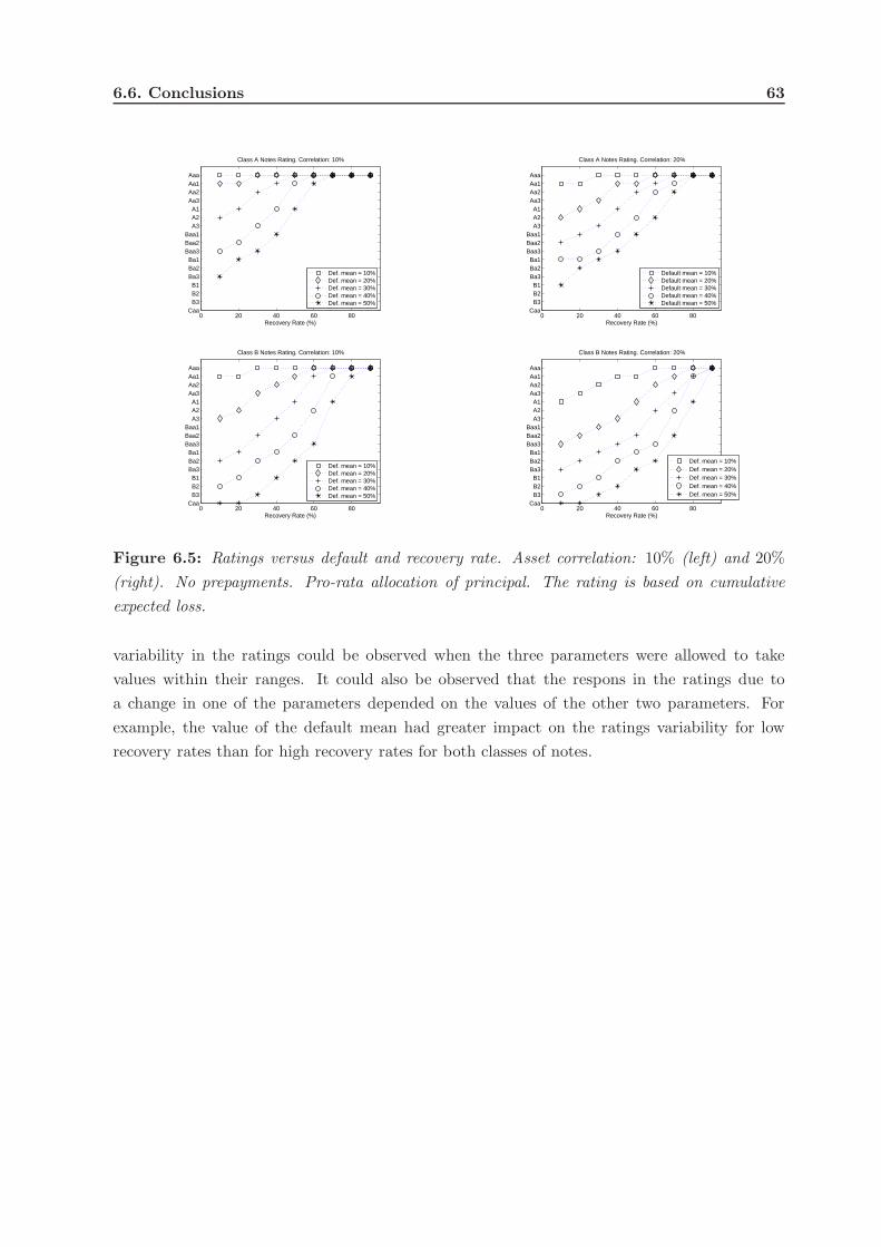
6.6. Conclusions 63

0 20 40 60 80Caa

B3B2B1

Ba3Ba2Ba1

Baa3Baa2Baa1

A3A2A1

Aa3Aa2Aa1Aaa

Class A Notes Rating. Correlation: 10%

Recovery Rate (%)

Def. mean = 10%Def. mean = 20%Def. mean = 30%Def. mean = 40%Def. mean = 50%

0 20 40 60 80Caa

B3B2B1

Ba3Ba2Ba1

Baa3Baa2Baa1

A3A2A1

Aa3Aa2Aa1Aaa

Class A Notes Rating. Correlation: 20%

Recovery Rate (%)

Default mean = 10%Default mean = 20%Default mean = 30%Default mean = 40%Default mean = 50%

0 20 40 60 80Caa

B3B2B1

Ba3Ba2Ba1

Baa3Baa2Baa1

A3A2A1

Aa3Aa2Aa1Aaa

Class B Notes Rating. Correlation: 10%

Recovery Rate (%)


0 20 40 60 80Caa

B3B2B1

Ba3Ba2Ba1

Baa3Baa2Baa1

A3A2A1

Aa3Aa2Aa1Aaa

Class B Notes Rating. Correlation: 20%

Recovery Rate (%)


Figure 6.5: Ratings versus default and recovery rate. Asset correlation: 10% (left) and 20%


expected loss.

variability in the ratings could be observed when the three parameters were allowed to take

values within their ranges. It could also be observed that the respons in the ratings due to

a change in one of the parameters depended on the values of the other two parameters. For

example, the value of the default mean had greater impact on the ratings variability for low

recovery rates than for high recovery rates for both classes of notes.

Chapter 7

Global Sensitivity Analysis for ABS

7.1 Introduction

In the previous chapter we looked at the ratings variability due to model choice and parameter

values. In the present chapter we are going to investigate the ratings parameter sensitivity

further by applying global sensitivity analysis techniques. We address the issue of identifying

the main sources of uncertainties for structured finance ratings. Sensitivity analysis is a powerful

methodology for analysing how uncertainty in the output can be allocated to different sources

of uncertainty in the inputs, see for example Saltelli et al (2008) for an introduction to global

sensitivity analysis.

Global sensitivity analysis is based on exploring the space of all possible combinations for

the input parameters as effective as possible. We propose to work with a screening method

called the elementary effect method. The aim of screening methods is to identify the subsets of

influential and non-influential input factors using a small number of model evaluations.

This chapter is mainly based on results first presented in Campolongo et al (2010), which

contains a much more extensive analysis than what is presented here.

7.2 The ABS Structure

We will assume a static and homogeneous collateral pool with the characteristics presented in

Table 7.1.

This collateral pool is backing three classes of notes: A (senior), B (mezzanine), and C

(junior). The details of the notes are given in Table 7.2 together with other structural charac-

teristics. To this basic liability structure we have added a cash reserve account. The allocation of

principal due to be paid to the notes is done sequentially. Note that this refers to the calculation

of principal due to be paid. The actual amount of principal paid to the different notes depends

on the available funds at the relevant level of the waterfall.

The waterfall of the structure is presented in Table 7.3. The waterfall is a so called com-

bined waterfall where the available funds at each payment date constitutes of both interest and

65

66 Chapter 7 - Global sensitivity analysis for ABS

Collateral

Number of loans 2000

Initial principal amount 100,000,000

Weighted average maturity 5 years

Weighted average coupon (per annum) 9%

Amortisation Level-Pay

Payment frequency Monthly

Table 7.1: Collateral characteristics.

Liabilities

Class Initial Interest Credit

of Principal Rate enhance-

Notes Amount (per annum) ment (%)

A 80,000,000 1% 20%

B 14,000,000 2% 6%

C 6,000,000 4% 0%

General Features

Final Maturity 10 years


Principal allocation Sequential

Shortfall rate (per annum) Applicable note coupon

Senior expenses

Issuer fees 1% of Outstanding Pool Balance

Servicer fees 1% of Outstanding Pool Balance


Shortfall rate (per annum) 20%

Cash reserve

Target amount 1% of Outstanding Pool Balance

Minimum required amount 0% of Outstanding Pool Balance

Table 7.2: Liability and structural characteristics.

principal collections.

7.3 Cashflow Modelling

The cashflow from the pool is modelled as described in Chapter 2. The cash collections each

month from the asset pool consists of interest payments and principal collections (scheduled

repayments). Note that there are no unscheduled prepayments in the pool. These collections

7.4. Modelling Defaults 67

Waterfall


1) Issuer expenses

2) Servicer expenses

3) Class A interest

4) Class B interest




8) Class C interest

9) Class C principal

10) Class C additional returns

Table 7.3: The waterfall used in the analysis.

constitutes together with the principal balance of the reserve account Available Funds at the

end of each month.

7.4 Modelling Defaults

We model defaults in the asset pool by using the Logistic model that was treated in Section

3.2.3 and repeated here for convenience:

F (t) =a

1 + be−c(t−t0), 0 ≤ t ≤ T, (7.1)

where a, b, c, and t0 are positive constants. Parameter a controls the right endpoint of the

curve.

As explained in Section 3.2.3 the Logistic model can easily be combined with a Monte Carlo

based scenario generator to generate default scenarios by sampling a value for a from a given

default distribution. In this chapter the Normal Invers distribution will be used to describe the

cumulative portfolio default rate (PDR) distribution at the maturity of the structure:

FPDR(y) = P [PDR < y] = Φ

(√1 − ρΦ−1(y) − Kd(T )√

ρ

)

(7.2)

where 0% ≤ y ≤ 100% and Kd(T ) = Φ−1(p(T )). The default distribution in (7.2) is a function

of the obligor correlation, ρ, and the default probability, p(T ), which are unknown and unob-

servable. Instead of using these parameters as inputs it is common to fit the mean and standard

deviation of the distribution to the mean and standard deviation estimated from historical data,

see discussion in Appendix A.


7.4.1 Quasi-Monte Carlo Algorithm

To perform the sensitivity analysis we need to run our rating algorithm multiple of times with

different parameter settings as will be explained in Section 7.5. For each run of the rating

algorithm we are using Monte Carlo simulation to calculate the expected loss and the expected

average life of the notes. To speed up the sensitivity analysis we are using Quasi-Monte Carlo

simulations based on Sobol sequences.1 (See Kucherenko (2008), Kucherenko et al (2010),

Kucherenko (2007), and Kucherenko et al (2000) for more information on Sobol sequences and

their applications.)

7.5 Sensitivity Analysis - Elementary Effects

A very efficient method within the screening methods in identifying important factors with

few simulations is the elementary effects method (EE method). It is very simple, easy to

implement and the results are clear to be interpreted. It was introduced in Morris (1991) and

has been refined by Campolongo and co-workers in Campolongo et al (2007). Because of the

ABS structure’s complexity it is computationally expensive and EE method is very well suited

for the sensitivity analysis of the ABS model’s output.

The elementary effect (EE) of a specific input factor is the difference in the model output

when this particular input factor is changed, while the rest of the input factors are kept constant.

The method is thus based on one-at-a-time sensitivity analysis. However, in the EE method the

one-at-a-time analysis is done many times for each input, each time under different settings of the

other input factors, and the sensitivity measures are calculated from the empirical distribution

of the elementary effects.

Let us assume that there are k uncertain input parameters X1,X2, . . . ,Xk (assumed to be

independent) in our model. Examples of input parameters are the mean and standard deviation

of the default distribution.

To each input factor we assign a range and a distribution. For example, we could assume

that X1 is the mean of the default distribution and that it takes values in the range [5%, 30%]

uniformly, that is, each of the values in the range is equally likely to be chosen. We could of

course use non-uniform distributions as well, for example, an empirical distribution.

These input parameters and their ranges create an input space of all possible combinations

of values for the input parameters. To apply the EE method we map each of the ranges to the

unit interval [0, 1] such that the input space is completely described by a k-dimensional unit

cube.

The original method by Morris provides two sensitivity measures for each input factor i =

1, 2, . . . k:

1 We have been using the ’sobolset’ class (with the ’MatousekAffineOwen’ scramble algorithm) and ’RandStream’

class (with the ’mrg32k3a’ generator algorithm) in MATLABr for generating Sobol sequences and pseudo

random numbers, respectively.

7.5. Sensitivity Analysis - Elementary Effects 69

• µi used to detect input factors with an important overall influence on the output;

• σi used to detect input factors involved in interaction with other factors or whose effect is

not linear.

In order to estimate the sensitivity measures, a number of elementary effects must be calculated

for each input factor. Morris suggested an efficient design that builds r trajectories in order to

compute r elementary effects. Each trajectory is composed by (k + 1) points in the input space

such that each input factor changes value only once. A characteristic of this design is that the

points on the same trajectory are not independent and in fact two consecutive points differ only

in one component. Points belonging to different trajectories are independent since the starting

points of the trajectories are independent.

Once a trajectory has been generated, the model is evaluated at each point of the trajectory

and one elementary effect for each input factor can be computed. The EE of input factor i is

either:

EEi(X(l)) =

Y(

X(l+1))

− Y(

X(l))

∆(7.3)

if the ith component of X(l) has been increased by ∆ or

EEi(X(l)) =

Y(

X(l))

− Y(

X(l+1))

∆(7.4)

if the ith component of X(l) has been decreased by ∆, where Y(

X(l))

is the model output of

interest calculated in the point X(l) on the trajectory.

By randomly sampling r trajectories, r elementary effects can be estimated for each input.

Usually the number of trajectories (r) depends on the number of factors, on the computational

cost of the model, and on the number of levels (p) that each input can vary across. It has been

proven that the best choice is to let p be an even integer and ∆ to be equal to p2(p−1) (see Saltelli

et al (2004) and Saltelli et al (2008)).

The sensitivity measures are defined as the mean and the standard deviation of the distri-

bution for the elementary effects of each input:

µi =

∑rj=1 EEj

i

r(7.5)

and

σi =

√

∑rj=1(EEj

i − µi)2

r − 1. (7.6)


When considering elementary effects with opposite signs related to the ith factor, the effects may

cancel each other out generating a low µi value. To overcome this problem Morris recommends

to consider both µi and σi simultaneously in order to be able to draw some conclusions on the

factor importance.

In Campolongo et al (2007), two improvements of the original EE method are proposed.

Firstly, the sampling strategy to generate the trajectories is constructed such that optimized

trajectories are generated. A large number of different trajectories (e.g. 1000) is constructed

and then r of them are selected in order to get the maximum spread in the input space. (See

Campolongo et al (2007) for the all details about the design that builds the r trajectories

of (k + 1) points in the input space.) The second improvement is the introduction of a new

sensitivity measure based on the absolute values of the elementary effects:

µ∗

i =

∑rj=1 |EEj

i |r

. (7.7)

This new sensitivity measure overcomes the cancelation effect mentioned earlier and can alone

be used to assess the importance of each factor in the model.

Section 7.6 presents the results obtained by applying this methodology to the ABS model.

7.6 The SA Experiment

In order to apply the elementary effect method we first have to identify the outputs we want

to study and which input factors that are controllable (i.e. know) and which are uncontrollable

(i.e. unknown). We also have to identify suitable ranges for the uncontrollable input factors.

The sensitivity analysis (SA) is performed on the structure presented in Section 7.2 and the

default model presented in Section 7.3. The fundamental output in our study is the rating of the

ABSs. These ratings are derived from the Expected Average Life and the Expected Loss

of the notes. Because of that, these two quantities are the outputs the SA should investigate in

order to assess the influence of the unknown inputs in the ABS ratings.

Without loss of generality, the investor is assumed to be informed about the collateral pool’s

characteristics and the structural characteristics given in Table 7.1 and Table 7.2, respectively,

and the waterfall in Table 7.3. These are treated as controllable input factors.

Assuming the default distribution of the pool to follow a Normal Inverse distribution and the

default curve to be modelled by the Logistic model, the uncertain input factors in the SA are not

related to the model choice but to the parameters of the cumulative default rate distribution,

the default timing (the Logistic function) and the recoveries:

• the mean (µcd) and the standard deviation (σcd) of the Normal Inverse distribution;

• b, c, and t0 of the Logistic Function;

• the recovery rate (RR) and the recovery lag (TRL).

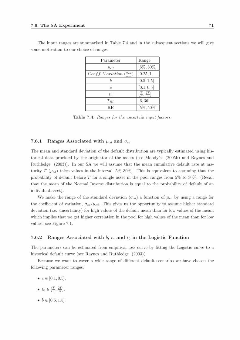
7.6. The SA Experiment 71

The input ranges are summarised in Table 7.4 and in the subsequent sections we will give

some motivation to our choice of ranges.

Parameter Range

µcd [5%, 30%]

Coeff. V ariation (σcd

µcd) [0.25, 1]

b [0.5, 1.5]

c [0.1, 0.5]

t0 [T3 , 2T3 ]

TRL [6, 36]

RR [5%, 50%]

Table 7.4: Ranges for the uncertain input factors.

7.6.1 Ranges Associated with µcd and σcd

The mean and standard deviation of the default distribution are typically estimated using his-

torical data provided by the originator of the assets (see Moody’s (2005b) and Raynes and

Ruthledge (2003)). In our SA we will assume that the mean cumulative default rate at ma-

turity T (µcd) takes values in the interval [5%, 30%]. This is equivalent to assuming that the

probability of default before T for a single asset in the pool ranges from 5% to 30%. (Recall

that the mean of the Normal Inverse distribution is equal to the probability of default of an

individual asset).

We make the range of the standard deviation (σcd) a function of µcd by using a range for

the coefficient of variation, σcd/µcd. This gives us the opportunity to assume higher standard

deviation (i.e. uncertainty) for high values of the default mean than for low values of the mean,

which implies that we get higher correlation in the pool for high values of the mean than for low

values, see Figure 7.1.

7.6.2 Ranges Associated with b, c, and t0 in the Logistic Function

The parameters can be estimated from empirical loss curve by fitting the Logistic curve to a

historical default curve (see Raynes and Ruthledge (2003)).

Because we want to cover a wide range of different default scenarios we have chosen the

following parameter ranges:

• c ∈ [0.1, 0.5];

• t0 ∈ [T3 , 2T3 ];

• b ∈ [0.5, 1.5].


0.2 0.3 0.4 0.5 0.6 0.7 0.8 0.9 10

0.1

0.2

0.3

0.4

0.5

0.6

0.7

Coefficient of variation (σ/µ)

Cor

rela

tion

Normal Inverse distribution: Implied correlation

Def. mean = 0.05Def. mean = 0.10Def. mean = 0.20Def. mean = 0.30

Figure 7.1: Implied correlation versus coefficient of variation

Inspecting the behavior of the Logistic functions in Figure 7.2 provides some insight to the

possible scenarios generated with these parameter ranges and gives an intuitive understanding

of the different parameters influence on the shape of the curve.

7.6.3 Ranges Associated with Recovery Rate and Recovery Lag

Recovery rates and recovery lags are very much dependent on the asset type in the underlying

pool and the country where they are originated. For SME loans, for example, Standard and

Poor’s made the assumption that the recovery lag is between 12 months to 36 months depending

on the country (see Standard and Poor’s (2004a)). Moody’s uses different recovery rate ranges

for SME loans issued in, for example, Germany (25%−65%) and Spain (30%−50%), see Moody’s

(2009a).

The range associated with recovery lag TRL has been fixed to be equal to [6, 36] months and

with the recovery rate to be equal to [5%, 50%].

7.7 Numerical Results

The fundamental output in the ABS model is the rating that addresses the expected loss a note

investor might suffer. With screening the input space of the ABS model using the elementary

effect method we aim at answering the questions: Is the rating of the ABS reliable? Where is

the uncertainty coming from, i.e. which input factors are more important in determining the

uncertainty in the rating response? In this section we present results concerning the sensitivity

measures µ∗ and σ and refer to Campolongo et al (2010) for the full study.

Having estimated both the expected loss and the expected average life we can map these

values into Moody’s ratings using the Moody’s Idealised Cumulative Expected Loss Table (see

Moody’s (2000b)).

7.7. Numerical Results 73

0 10 20 30 40 50 600

0.1

0.2

0.3

0.4

0.5

0.6

0.7

0.8

0.9

1

Logistic function: a=1; b=0.5; t0=15; T=60.

Time (months)

F(t

)

c = 0.10c = 0.20c = 0.50

0 10 20 30 40 50 600

0.02

0.04

0.06

0.08

0.1

0.12

0.14


Time (months)

dF(t

)/dt

c = 0.10c = 0.20c = 0.50

0 10 20 30 40 50 600

0.1

0.2

0.3

0.4

0.5

0.6

0.7

0.8

0.9

1


c = 0.10c = 0.20c = 0.50

0 10 20 30 40 50 600

0.02

0.04

0.06

0.08

0.1

0.12

0.14


c = 0.10c = 0.20c = 0.50

0 10 20 30 40 50 600

0.1

0.2

0.3

0.4

0.5

0.6

0.7

0.8

0.9

1


Time (months)

F(t

)

c = 0.10c = 0.20c = 0.50

0 10 20 30 40 50 600

0.02

0.04

0.06

0.08

0.1

0.12

0.14


Time (months)

dF(t

)/dt

c = 0.10c = 0.20c = 0.50

0 10 20 30 40 50 600

0.1

0.2

0.3

0.4

0.5

0.6

0.7

0.8

0.9

1


c = 0.10c = 0.20c = 0.50

0 10 20 30 40 50 600

0.02

0.04

0.06

0.08

0.1

0.12

0.14


c = 0.10c = 0.20c = 0.50

Figure 7.2: The Logistic function and its derivative for different values of b, c and t0. Param-

eter values: a = 1 and T = 60.

We apply the elementary effect method improved by Campolongo et al (2007) with r = 10

optimized trajectories of p = 4 points. This choice has been demonstrated to produced valuable

results in a general application of the sensitivity analysis.2 Having k = 7 input parameters, a

2 Saltelli et al (2004), p. 102.


total number of 80 (N = r(k + 1)) model evaluations have to be performed. The ABS model

runs 214 times for each evaluation, in order to guarantee the convergence. Thus, we simulate

214 scenarios to get the ratings for each parameter setting of the input factors.

7.7.1 Uncertainty Analysis

The empirical distribution of the ratings on each note can be used to obtain information on the

uncertainty in the model (see Figure 7.3).

The A notes rating seems to be reliable and the performance is of high quality. We get good

ratings with low degree of risk at 80% of the time and the best rating, Aaa, is obtained at 54%

of time. The B notes ratings are not reliable because of the oscillation between ’Aaa’ rating and

’Unrated’. The C notes are considered to be unrated at 46% of time so that the investor should

be aware that the C notes are highly speculative and typically may suffer significant losses.

Aaa Aa1 Aa2 Aa3 A1 A2 A3 Baa1Baa2Baa3 Ba1 Ba2 Ba3 B1 B2 B3 Caa Unr.0

20

40

60

80A notes


20

40

60

80

Fre

quen

cy fo

r 80

sim

ulat

ions

B notes


20

40

60

80

Moodys Ratings

C notes

Figure 7.3: Moody’s Ratings empirical distribution obtained by 80 simulations


0

1

2

3

4

5

6

7x 10

−3

M

ean

Norm

al In

vers

e

Coeff.

Var

iation

R

ecov

ery R

ate

Recov

ery L

ag

b o

f Log

istic

Functi

on

c o

f Log

istic

Functi

on

t0 o

f Log

istic

Functi

on

A notes

Mus

tar

with

res

pect

to th

e E

xpec

ted

Loss

0

0.2

0.4

0.6

0.8

1

1.2

1.4

M

ean

Norm

al In

vers

e

Coeff.

Var

iation

R

ecov

ery R

ate

Recov

ery L

ag

b o

f Log

istic

Functi

on

c o

f Log

istic

Functi

on

t0 o

f Log

istic

Functi

on

A notes

Mus

tar

with

res

pect

to th

e E

xpec

ted

Ave

rage

Life

Figure 7.4: Bar plots of the µ∗ values for the A notes

7.7.2 Sensitivity Measures µ∗ and σ

In order to investigate where the uncertainty in the ratings comes from we focus on the expected

loss and the expected average life. The SA provides two fundamental measures to rank each

input factor in order of importance, the µ∗ and σ for the elementary effects of each input. In

Figure 7.4, Figure 7.5, and Figure 7.6 bar plots of µ∗ are presented to visually depict the rank

of the different input factors. The input factors nonlinear effects are illustrated in Figure 7.7,

Figure 7.8, and Figure 7.9 with the help of scatter plots of (µ∗, σ).

At a first look at the bar plots it is clear that the least influential factors across all outputs are

the recovery lag and the Logistic function’s b parameter and hence they could be fixed without

affecting the variance of the outputs of interest and therefore the ratings to a great extent.

Among the influential parameters the mean of the default distribution (µcd) is clearly the

most influential input parameter over all for all three notes. It is characterized by high µ∗ values

for both the expected loss and the expected average life of all the notes, confirming the strong

influence the mean default rate assumption has on the assessment of ABSs. The only exception

from ranking the mean default rate as the most influential input factor is the expected loss of

the A notes. Here the coefficient of variation is ranked the highest with the recovery rate as

second and the mean default rate as third.

The input factors with the highest µ∗ values for expected loss and expected average life,


respectively are the same for the B notes with just small changes of the ranking. The same

feature holds true also for the C notes. For these two classes of notes the mean default rate is

the absolutely most influential input factor. For the A notes the ranking of the input factors

differs more significantly between expected loss and expected average life. For the expected loss

the two parameters of the default distribution together with the recovery rate are clearly the

most influential. For the expected average life the Logistic function’s c and t0 should be counted

as influential together with default distributions parameters and the recovery rate.

In the scatter plots in Figures 7.7 – 7.9 it is visible that the most influential factors also have

the highest values of σ which indicate strong nonlinear effects and/or interactions with other

factors.

0

0.05

0.1

0.15

0.2

0.25

Mean Normal In

verse

Coeff. Variation

R

ecovery Rate

R

ecovery Lag

b

of Logistic Function

c


t0


B notes

Mus

tar

with

res

pect

to th

e E

xpec

ted

Loss

0

2

4

6

8

10

12

14

16

18

20

Mean Normal In

verse

Coeff. Variation

R

ecovery Rate

b


c


t0


B notes

Mus

tar

with

res

pect

to th

e E

xpec

ted

Ave

rage

Life

R

ecovery Lag

Figure 7.5: Bar plots of the µ∗ values for the B notes


0

0.1

0.2

0.3

0.4

0.5

0.6

0.7C notes

Mean Normal In

verse

Coeff. Variation

R

ecovery Rate

R

ecovery Lag

b


c


t0


Mus

tar

with

res

pect

to th

e E

xpec

ted

Loss

0

5

10

15

20

25

30

35

40

Mean Normal In

verse

Coeff. Variation

R

ecovery Rate

R

ecovery Lag

b


c


t0


C notes

Mus

tar

with

res

pect

to th

e E

xpec

ted

Ave

rage

Life

Figure 7.6: Bar plots of the µ∗ values for the C notes

0 1 2 3 4 5 6 7

x 10−3

0

0.001

0.002

0.003

0.004

0.005

0.006

0.007

0.008

0.009

0.01

mu

coeff.Var

RR

R.Lag

b

c

t0

mu*

sig

ma

Expected Loss for A notes

0.2 0.4 0.6 0.8 1 1.2 1.4 1.60

0.001

0.002

0.003

0.004

0.005

0.006

0.007

0.008

0.009

0.01

mu

coeff.Var

RR

RR

b

c

t0

mu*

sig

ma

Expected Average Life for A notes

Figure 7.7: Scatter plots of the sensitivity measures µ∗ and σ for the Expected Loss and Expected

Average Life in the A notes.


0 0.05 0.1 0.15 0.2 0.250

0.05

0.1

0.15

0.2

0.25

mu

coeff.Var

RR

R.Lag

b

c

t0

mu*

sig

ma

Expected Loss for B notes

0 5 10 15 200

0.05

0.1

0.15

0.2

0.25

mu

coeff.Var

RR

R.Lag

b

c

t0

mu*sig

ma

Expected Average Life for B notes


Average Life in the B notes.

0 0.1 0.2 0.3 0.4 0.5 0.6 0.70

0.05

0.1

0.15

0.2

0.25

0.3

0.35

mu

coeff.Var

RR

R.Lag b

c

t0

mu*

sig

ma

Expected Loss for C notes

0 5 10 15 20 25 30 35 400

0.05

0.1

0.15

0.2

0.25

0.3

0.35

mu

coeff.Var

RR

R.Lag b

c

t0

mu*

sig

ma

Expected Average Life for C notes


Average Life in the C notes.

7.8. Conclusions 79

7.8 Conclusions

In this chapter, we have shown how global sensitivity analysis can be used to analyse the

main sources of uncertainty in the ratings of asset-backed securities (ABSs). Due to the fact

that deriving ratings for ABSs is computationally expensive, the elementary effect method was

chosen for the analysis. The elementary effect method was applied to a test example consisting

of a large homogeneous pool of assets backing three classes of notes (senior, mezzanine and

junior).

The result of the sensitivity analysis experiment has led to the conclusion that the least

influential factors across all outputs are the recovery lag and the Logistic function’s b parameter.

Hence they could be fixed without affecting the variance of the outputs of interest and therefore

the ratings to a great extent.

The mean of the default distribution (µcd) was found to be the most influential input pa-

rameter among all inputs for all three notes. It is characterized by high µ∗ values for both the

expected loss and the expected average life of all the notes, confirming the strong influence the

mean default rate assumption has on the assessment of ABSs. The only exception from ranking

the mean default rate as the most influential input factor could be found for the expected loss

of the A notes. Here the coefficient of variation is ranked the highest with the recovery rate as

second and the mean default rate as third.

It was further indicated that the most important input factors contributes to the rating

uncertainty in a nonlinear way and/or with possible interactions between several of the factors.

Chapter 8

Summary

8.1 Introduction to Asset Backed Securities

Asset-Backed Securities (ABSs) are financial instrument backed by pools of assets. ABSs are

created through a securitisation process, where assets are pooled together and the liabilities

backed by these assets are tranched such that the ABSs have different seniority and risk-return

profiles.

Due to the complex nature of securitisation deals there are many types of risks that have to

be taken into account. The risks arise from the collateral pool, the structuring of the liabilities,

the structural features of the deal and the counterparties in the deal. The main types of risks are

credit risk, prepayment risk, market risks, reinvestment risk, liquidity risk, counterparty risk,

operational risk and legal risk.

The quantitative analysis of an ABS is done through the modelling of the cashflows within

the ABS deal. The modelling consists of two steps. The first step is to model the cash collections

from the asset pool, which depends on the behaviour of the pooled assets. This can be done in

two ways: with a top-down approach, modelling the aggregate pool behaviour; or with a bottom-

up or loan-by-loan approach modelling each individual loan. It is in this step quantitative models

and assumptions are needed. The second step is to model the distribution of the cash collections

to the note holders, the issuer, the servicer and other transaction parties. This distribution of

the cash collection, the so called priority of payments or waterfall, is described in detail in the

Offering Circular or Deal Prospectus.

The cash collections from the asset pool consist of interest collections and principal collections

(both scheduled repayments, unscheduled prepayments and recoveries). There are two parts of

the modelling of the cash collections from the asset pool. Firstly, the modelling of performing

assets, based on asset characteristics such as initial principal balance, amortisation scheme,

interest rate and payment frequency and remaining term. Secondly, the modelling of the assets

becoming delinquent, defaulted and prepaid, based on assumptions about the delinquency rates,

default rates and prepayment rates together with recovery rates and recovery lags.

To be able to model cash collections from the asset pool it is needed to generate default and

81

82 Chapter 10 - Summary and Conclusions

prepayment scenarios. We divide the default and prepayment models into two groups, deter-

ministic (Chapter 3) and stochastic models (Chapter 4). The deterministic models are simple

models with no built in randomness, i.e., as soon as the model parameters are set the evolution

of the defaults and prepayments are know for all future times. The stochastic models are more

advanced, based on stochastic processes and probability theory. By modelling the evolution of

defaults with stochastic processes we can achieve three objectives: stochastic timing of defaults;

stochastic monthly default rates; and correlation (between defaults, between prepayments and

between defaults and prepayments).

The quantitative models and approaches used today are either deterministic, in the sense

that the distribution of defaults or prepayments are certain as soon as the parameters of the

models are fixed and the cumulative default rate and prepayment rate, respectively, are chosen,

or they are stochastic and based on the Normal distribution. In the report a collection of

default and prepayment models are presented, ranging from very simple deterministic models

to advanced stochastic models. We have proposed a set of new stochastic models that are based

on more flexible distributions than the Normal, which take into account more extreme events.

8.2 Rating Agencies Methodologies

Two of the major rating agencies, Moody’s and Standard & Poor’s (S&P’s), methodologies for

rating securitisation transactions has also been studied (Chapter 5). The focus in the study has

been on their methodologies for rating SME (Small and Medium-sized Enterprizes) securitisation

transactions. The two rating agencies have two different meanings of their ratings. Moody’s

rating is an assessment of the expected loss that a class of notes may experience during a certain

time period, while S&P’s rating is an assessment of the probability of default of the class of notes

and addresses the likelihood of full and timely payment of interest and the ultimate payment of

principal.

Both Moody’s and S&P’s discriminate between granular and non-granular SME portfolios

and applies different approaches to the two categories.

For non-granular SME portfolios both rating agencies use a loan-by-loan or bottom-up ap-

proach and model each individual asset in the pool. Moody’s uses its CDOROMTM tool, which

uses Normal factor models (with dependence structure based on the Gaussian copula approach);

S&P’s is using its CDO Evaluatorr model, which is based on the Gaussian copula approach. In

both cases, thus, are the underlying mathematical tool to introduce dependence in the portfolios

the Gaussian copula approach. Monte Carlo simulations are used to generate defaults in the

asset pool and to derive a default distribution. The difference between the two methodologies

lies in the use of the tool or model.

In Moody’s methodology, the default scenario generated by each Monte Carlo simulation is

fed into the cash flow model and the losses on the ABSs are derived. This is done for a large

number of simulations and an estimate of the expected loss on each ABS is derived. The cash

flow analysis is thus an integrated part of the simulations. The expected losses are mapped to

8.3. Model Risk and Parameter Sensitivity 83

a rating for each ABS using Moody’s loss rate tables.

In S&P’s methodology, the Monte Carlo simulations generate a probability distribution of

potential portfolio default rates that is used to derive a set of scenario default rates (SDRs),

one for each rating level. Each SDR represents the maximum portfolio default rate that an

ABS with the desired rating should be able to withstand without default. These SDRs are then

used to create different stressed rating scenarios that are applied in a cash flow analysis, which

assesses if the ABS under consideration can withstand the stresses associated with the targeted

rating level and therefore can receive the corresponding rating level.

For granular SME portfolios, Moody’s uses its ABSROMTM tool, which uses a default rate

distribution to generate default scenarios and the corresponding likelihood of each scenario.

The default rate distribution’s mean and standard deviation is estimated using historical data

provided by the originator. Running a cash flow model with the different default scenarios,

stressing the default timing, the expected loss on the notes are calculated. S&P’s applies its

actuarial approach for granular SME portfolios, which is based on deriving base case default

and recovery rates from historical data in order to stress defaults over the life of the transaction

in different rating scenarios in a cash flow analysis.

8.3 Model Risk and Parameter Sensitivity

The models influence on the ratings of structured finance transactions were studied on a trans-

action with two classes of notes (Chapter 6). The findings can be summarised by saying that

model risk is omnipresent. The model risk was assessed by comparing three different default

models with a benchmark model, the Normal one-factor model. What could be observed for a

low cumulative default rate assumption (10%) was that there was no or just one notch difference

in rating for the senior notes and one to three notches difference for the junior notes, between

the models output. However, increasing the cumulative default rate to a high number (40%)

the rating differed with as much as three notches for the senior notes and four notches for the

junior notes. Thus, for high cumulative default rates the model risk becomes more significant.

The ratings sensitivity to the cumulative default rate assumption was also studied by analysing

the number of notches the ratings changed for a given default model when the default rate in-

creased. As could be expected, the ratings are very dependent on the cumulative default rate

assumption. For the junior notes the rating differed with as much as seven to eight notches,

when the cumulative default rate changes from 10% to 40%. For the senior notes the changes

were one to four notches.

In a second analysis we analysed the variability in the ratings related to uncertainty in the

mean default rate, asset correlation and recovery rate under the Normal one-factor model. Big

variability in the ratings could be observed when the three parameters were allowed to take

values within their ranges. It could also be observed that the respons in the ratings due to

a change in one of the parameters depended on the values of the other two parameters. For

example, the value of the default mean had greater impact on the ratings variability for low

84 Chapter 10 - Summary and Conclusions

recovery rates than for high recovery rates for both classes of notes.

8.4 Global Sensitivity Analysis

To further investigate the ABS ratings parameter sensitivity we have proposed to apply global

sensitivity analysis techniques (Chapter 7). Global sensitivity analysis is the study of how the

uncertainty in a model’s input affects the model’s output and investigates the relative importance

of each input in determining this uncertainty. In global sensitivity analysis the input parameters

take values in ranges given by the analyst. These input ranges creates an input space and an

aim with global sensitivity analysis is to explore this input space and analyse the model output’s

respons to different combinations of input parameter values. To identify which input parameters

are the most influential and which are non-influential a screening method is suitable for ranking

the input parameters in a computationally expensive problem as the rating of ABSs. We have

chosen to work with the elementary effect (EE) method, which is best practise among the

screening methods. The EE method explores the input space in an optimal way.

To illustrate the method we applied the EE method to an ABS structure with three classes

of notes: A (senior), B (mezzanine) and C (junior), backed by a pool of homogeneous assets,

which could default but not prepay. Prepayment was excluded to simplify the experiment. Seven

input parameters were assumed to be uncertain in the experiment: the mean and coefficient of

variation of the default distribution, three parameters controlling the default timing (modelled

by the Logistic function), and the recovery rate and the recovery lag. The output studied were

the expected loss (EL) and the expected weighted average life (EAL) of the notes. The result of

the experiment indicated that the default distributions parameters and the recovery rate were

the most influential inputs for both EL and EAL for all classes of notes. The recovery lag and

one of the parameters of the default timing were found to be non-influential.

The identification of an input parameter as non-influential gives an opportunity to simplify

the model by fix this parameter to a constant value within the parameter’s range (so called

factor fixing) without influencing the variability of the output of the model. On the other hand,

the categorisation of an input parameter as influential indicates that it requires careful analysis

of its range (so called factor prioritisation).

Appendix A

Large Homogeneous Portfolio

Approximation

A.1 The Gaussian One-Factor Model and the LHP Approxima-

tion

In the Gaussian one-factor model an obligor is assumed to default if the value of its creditwor-

thiness is below a pre-specified value. The creditworthiness of an obligor is modeled through a

latent variable:

Zn =√

ρX +√

1 − ρXn, n = 1, 2, ..., N, (A.1)

where X is the systemic factor and Xn with n = 1, 2, ..., N are the idiosyncratic factors; all

assumed to be standard normal random variables with mean zero and unit variance and ρ is the

correlation between two assets:


The nth loan defaulted by time t if

Zn ≤ Kdn(t),

where Kdn(t) is the time dependent default barrier. Under the assumption of the homogenous

pool, each asset behaves as the average of the assets in the pool and we can set Kdn(t) = Kd(t)

for the all n. The default barrier can be chosen such that:

P (Zn ≤ Kd(T )) = p(T ), (A.2)

where p(T ) is the probability of default of a single obligor in the pool by maturity T . It implies

Kd(T ) = Φ−1(p(T )).

The cumulative portfolio default rate is given by:

PDR(T ) =

N∑

n=1

Dn(T )

N(A.3)

85

86 Appendix A: Large Homogeneous Portfolio Approximation

where Dn(T ) is the default indicator of asset n. The default indicator Dn(T ) equals one (with

probability p(T )) if asset n defaulted by time T and zero otherwise.

The expected value of the portfolio default rate at time T is

E[PDR(T )] = E[ 1N

∑Nn=1 Dn(T )]

= 1N

∑Nn=1 E[Dn(T )]

= E[D1(T )]

= P (D1(T ) = 1)

= P (Z1 ≤ Kd(T )) = p(T ),

(A.4)

where the third equality follows by the homogeneous portfolio assumption and the last equality

holds by definition. Thus under the homogeneous portfolio assumption the portfolio default rate

mean is equal to the individual loan’s probability of default p(T ).

The default indicators in (A.3) are correlated and we can not use the Law of Large numbers

to derive a limiting distribution. However, conditional on the common factor X, the default

indicators are independent and we can apply the Law of Large Numbers.

Conditional on the common factor the portfolio default rate at time T is given by

PDR(T ;X = x) =

N∑

n=1

Dn(T ; X = x)

N(A.5)

where Dn(T ; X = x) is the default indicator of asset n given the systematic factor X.

By the Law of Large Numbers, as N tends to infinity we get:

PDR(T ;X = x) →N→∞

E[Pcd|X = x] =1

N

N∑

n=1

p(x) =1

NNp(x) = p(T, x), (A.6)

where p(T, x) is the default probability for an individual asset given X = x:

p(T, x) = P (Zn ≤ Kd(T )|X = x)

= P (√

ρX −√

1 − ρXn ≤ Kd(T )|X = x)

= Φ

(

Kd(T ) −√ρx√

1 − ρ

)

.

(A.7)

A.2. Calibrating the Distribution 87

It follows that the distribution of PDR(T ;X) is1:

FPDR(T ;X)(y) = P (PDR(T ;X) < y)

= P (p(X) < y)

= P

(

Φ

(

Kd(T ) −√ρX√

1 − ρ

)

< y

)

= P

(

X >Kd(T ) −√

1 − ρΦ−1(y)√ρ

)

.

(A.8)

Using the symmetry of the normal distribution, we get:

FLHPPDR(T ;X)(y) = P (PDR(T ;X) < y) = Φ

(√1 − ρΦ−1(y) − Kd(T )√

ρ

)

(A.9)

where 0% ≤ y ≤ 100% and Kd(T ) = Φ−1(p(T )). Note that the right hand side of (A.9)

is independent of the systemic factor X. The distribution in (A.9) is sometimes called the

Normal Inverse distribution, see, for example, Moody’s (2003).

Thus for a reasonably large homogeneous portfolio we can use the distribution in (A.9) as

an approximation to the portfolio default rate distribution.

We illustrate in Figure A.1 the portfolio default rate distribution’s dependence on the corre-

lation parameter ρ, under the assumption that the default mean is 30%. As can be seen from the

plots, under a low correlation assumption the PDR distribution will have a bell shaped form, but

as the asset correlation increases the mass of the distribution is shifted towards the end points

of the PDR interval, increasing the likelihood of zero or a very small fraction of the portfolio

defaulting and the likelihood of the whole portfolio defaulting. This is natural since a very high

correlation (close to one) means that the loans in the pool are likely to either survive together

or default together. In general, it can be said that the PDR distribution becomes flatter and

more mass is shifted towards the tails of the distribution when the default mean is increased.

A.2 Calibrating the Distribution

The default distribution in (A.9) is a function of the obligor correlation, ρ, and the default

probability, p(T ), which are unknown and unobservable. Instead of using these parameters as

inputs it is common to fit the mean and standard deviation of the distribution to the mean

and standard deviation, respectively, estimated from historical data (see, for example, Moody’s

(2005b) and Raynes and Ruthledge (2003)). Let us denote by µcd and σcd the estimated mean

and standard deviation, respectively.

The mean of the distribution is equal to the probability of default for a single obligor, p(T ),

so p(T ) = µcd. As a result there is only one free parameter, the correlation ρ, left to adjust to

fit the distribution’s standard deviation to σcd, which can be done numerically by minimising

σ2cd − V arρ(PDR(T )), where the subscript is used to show that the variance is a function of ρ.

1 The above convergence is in probability, which implies convergence in distribution.

88 Appendix A: Large Homogeneous Portfolio Approximation

Figure A.1: Portfolio default rate versus correlation. Large homogeneous portfolio approxima-

tion. Left panel: correlation between 1% and 90%. Right panel: correlation between 1% and

50%. Mean default rate: 30%.

0.2 0.3 0.4 0.5 0.6 0.7 0.8 0.9 10

0.1

0.2

0.3

0.4

0.5

0.6

0.7

Coefficient of variation (σ/µ)

Cor

rela

tion

Normal Inverse distribution: Implied correlation

Def. mean = 0.05Def. mean = 0.10Def. mean = 0.20Def. mean = 0.30

Figure A.2: Implied correlation for different values of mean and coefficient of variation (stan-

dard deviation divided by mean) equal to 0.25, 0.5, 0.75, 1.0 and 1.25.

Looking at the correlation values given in Figure A.2 and the density plots in Figure A.1 one

can see that the corresponding default distributions will have very different shapes. Ranging

from bell shaped curves to very heavy tailed ones with the mass almost completely concentrated

at zero and one.

It is important to understand that the behavior of the correlation and the default probability

shown in Figure A.2 should not be taken as a general rule. The graphs show the result of fitting

the distribution to means and standard deviations in the distribution’s “comfort zone”, i.e, values

that will give good fits. (The root mean squared error is of the order of magnitude of 10−11 for

the shown results.) For combinations of the default mean and the coefficient of variation that

result in an implied correlation equal to one the calibration will stop since it cannot improve

the root mean squared error, which in these situations will be much larger than for the values

shown in Figure A.2.

Bibliography

Albrecher, H., Ladoucette, S. and Schoutens, W. (2006), A Generic One-Factor Levy Model for

Pricing Synthetic CDOs, Advances in Mathematical Finance, M. Fu, R. Jarrow, J. Yen, R.J.

Elliott (eds.), pp. 259-278, Birkhauser, Boston.

Altman, E.I., Brady, B., Resti, A., and Sironi, A. (2005), The Link Between Default and Recov-

ery Rates: Theory, Empirical Evidence, and Implications, Journal of Business, Vol. 78, nr.

6.

Bank for International Settlements (2005) The role of ratings in structured finance: issues and

implications.

Campolongo, F., Cariboni, J. and Saltelli, A. (2007), An effective screening design for sensitivity

analysis of large models, Enviromental Modelling & Software, Vol. 22, pp. 1509–1518.

Campolongo, F., Di Girolamo, F., Jonsson, H., and Schoutens, W. (2010), Sense and sensitivity:

Global Sensitivity Analysis For ABS Ratings, working paper.

Fabozzi, F. J. and Kothari, V. (2008) Introduction to Securitization, John Wiley and Sons, Inc.,

Hoboken, New Jersey.

Geldilux-TS-2005 S.A., Offering Circular, 2005.

Jonsson, H., Schoutens, W., and van Damme, G. (2009), Modeling Default and Prepayment

using Levy Processes: an Application to Asset Backed Securities, Radon Series on Computa-

tional and Applied Mathematics, Vol. 8, pp. 183-204, de Gruyter, Berlin.

Jonsson, H. and Schoutens, W. (2010), Known and less known risks in asset-backed securities,

in D. Wigan (Ed.) Credit Derivatives - The March to Maturity, IFR Market Intelligence.

Li, A. (1995), A One-Factor Lognormal Markovian Interest Rate Model: Theory and Implemen-

tation, Advances in Futures and Options Research, Vol. 8.

Li, D. (2000), On Default Correlation: A Copula Function Approach, Journal of Fixed Income,

Vol. 9, pp. 43-54.

Merton, R. (1974), On the pricing of corporate debt: the risk structure of interest rates, J.

Finance, Vol. 29, pp. 449–470.

89

90 BIBLIOGRAPHY

Moody’s Investor Service (2000a), Contradictions in Terms: variations in Terminology in the

Mortgage Market, International Structured Finance, Special Report, 9 June 2000.

Moody’s Investor Service (2000b), The Lognormal Method Applied to ABS Analysis, Interna-

tional Structured Finance, Special Report, 27 July 2000.

Moody’s Investor Service (2001), The Combined Use of Qualitative Analysis and Statistical

Models in the Rating of Securitisations, International Structured Finance, Special Report, 11

July 2001.

Moody’s Investor Service (2003), The Fourier Transform Method - Technical Document, Working

Paper, 30 January 2003.

Moody’s Investor Service (2005a), Geldilux-TS-2005 S.A., International Structured Finance,

New-Issue Report, 17 June, 2005.

Moody’s Investor Service (2005b), Historical Default Data Analysis for ABS Transactions in

EMEA, International Structured Finance, Special Report, 2 December, 2005.

Moody’s Investor Service (2006a), Moody’s ABSROMTM v 1.0 User Guide, 22 May, 2006.

Moody’s Investor Service (2006b), Moody’s CDOROMTM v 2.3 User Guide, 1 June, 2006.

Moody’s Investor Service (2007a), Moody’s Approach to Rating CDOs of SMEs in Europe, In-

ternational Structured Finance, Rating Methodology, 1 February 2007.

Moody’s Investor Service (2007b), Information on EMEA SME Securitisations - Moody’s view

on granular SME loan receivable transactions and information guidelines, International Struc-

tured Finance, Special Report, 12 March 2007.

Moody’s Investor Service (2007c), Framework for De-Linking Hedge Counterparty Risks from

Global Structured Finance Cashflow Transactions, International Structured Finance, Rating

Methodology, 10 May 2007.

Moody’s Investor Service (2007d), Moody’s Approach to Rating Granular SME Transactions in

Europe, Middle East and Africa, International Structured Finance, Rating Methodology, 8

June 2007.

Moody’s Investor Service (2008), Revising Default/Loss Assumptions Over the Life of an

ABS/RMBS Transaction, International Structured Finance, Rating Methodology, 18 Decem-

ber, 2008.

Moody’s Investor Service (2009a), Refining the ABS SME Approach: Moody’s Probability of De-

fault assumptions in the rating analysis of granular Small and Mid-sized Enterprise portfolios

in EMEA, International Structured Finance, Rating Methodology, 17 March, 2009.

BIBLIOGRAPHY 91

Moody’s Investor Service (2009b), V Scores and Parameter Sensitivities in the EMA Small-to-

Medium Enterprise ABS Sector, International Structured Finance, Rating Methodology, 15

June, 2009.

Morris, R. D. (1991), Factorial Sampling Plans for Preliminary, Technometrics, Vol. 33, nb. 2,

pp. 161–174.

Raynes, S. and Rutledge, A. (2003), The Analysis of Structured Securities: Precise Risk Mea-

surement and Capital Allocation, Oxford University Press.

Saltelli, A., Tarantola, S., Campolongo, F., and Ratto, M. (2004), Sensitivity Analysis in Prac-

tice, Wiley.

Saltelli, A., Ratto, M., Andres, T., Campolongo, F., Cariboni, J., Gatelli, D., Saisana, M., and

Tarantola, S. (2008), Global Sensitivity Analysis: The Primer, Wiley.

Schoutens, W. and Cariboni, J. (2009), Levy Processes in Credit Risk, Wiley.

Kucherenko, S. (2007), Application of Global Sensitivity indices for measuring the effectiveness

of Quasi-Monte Carlo methods, Proc. of the Fifth International Conference on Sensitivity

Analysis of Model Output.

Kucherenko, S. (2008), High dimensional Sobol’s Sequences and their application, Technical

Report - www.broda.co.uk.

Kucherenko, S., Rodriguez-Fernandez, M. and Pantelides, C. and Shah, N. (2000), Monte Carlo

evaluation of derivative-based global sensitivity measures, Reliab. Eng. Syste. Saf., Vol. 94,

pp. 1135-1148.

Kucherenko, S., Feil, B. and Shah, N. and Mauntz, W. (2010), The identification of model

effective dimensions using global sensitivity analysis, Reliab. Eng. Syste. Saf..

Standard and Poor’s (2003), Standard & Poor’s Rating Methodology for CLOs Backed by Euro-

pean Small- and Midsize-Enterprise Loans, 30 January 2003.

Standard and Poor’s (2004a), Credit Risk Tracker Strengthens Rating Analysis of CLOs of

European SME Loans, 10 June 2004.

Standard and Poor’s (2004b), CDO Spotlight: General Cash Flow Analytics for CDO Securiti-

zations, 25 August 2004.

Standard and Poor’s (2005), CDO Evaluator Version 3.0: Technical Document, 19 December

2005.

Standard and Poor’s (2006a), Rating Methodology For CLOs Backed By German Participation

Rights, 25 April 2006.

92 BIBLIOGRAPHY

Standard and Poor’s (2006b), Update to General Cash Flow Analytics Criteria for CDO Secu-

ritizations, 17 October 2006.

Standard and Poor’s (2007a), Revised Framework For Applying Counterparty And Supporting

Party Criteria, 8 May 2007.

Standard and Poor’s (2007b), Principles-Based Methodology For Global Structured Finance Se-

curities, 29 May 2007.

Standard and Poor’s (2008a), Methodology: Update Counterparty Criteria For Derivatives: El-

igibility Of ’A-2’ Counterparties Removed in ’AAA’ Transactions, 22 October 2008.

Standard and Poor’s (2008b), CDO Evaluator 4.1 User Guide, 1 December 2008.

Standard and Poor’s (2009a), Methodology and Assumptions: Update To The Criteria For Rating

European SME Securitizations, 6 January 2009.

Standard and Poor’s (2009b), Summary And Highlights Of Proposed Changes To Our Global

Rating Methodology For Corporate Cash Flow And Synthetic CDOs, 17 March 2009.

Standard and Poor’s (2009c), Methodology and Assumptions: Update And Clarification To Coun-

terparty Criteria For Interest Rate Swap Counterparties In ’AAA’ Rated Transactions, 1 April

2009.

Standard and Poor’s (2009d), Standard and Poor’s Credit Rating Definitions, 4 August 2009.

Vasicek, O. (1987), Probability of Loss on Loan Portfolio, Technical Report, KMV Corporation,

1987.

BIBLIOGRAPHY 93

Quantitative assessment of securitisation deals · · 2011-01-03EURANDOM PREPRINT SERIES 2010-045...

Documents

Transcript of Quantitative assessment of securitisation deals · · 2011-01-03EURANDOM PREPRINT SERIES 2010-045...