Quantitative AES IV: Accuracy of the Numerical Evaluation of Peak Areas in AES using the Universal...

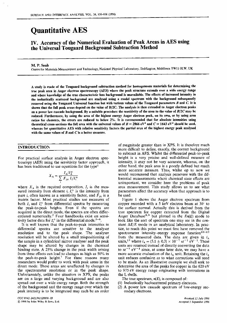
SURFACE AND INTERFACE ANALYSIS, VOL. %, 830-838 (1996)

Quantitative AES IV. Accuracy of the Numerical Evaluation of Peak Areas in AES using the Universal Tougaard Background Subtraction Method

M. P. Seah Centre for Materials Measurement and Technology, National Physical Laboratory, Teddington, Middlesex TW11 OLW, UK

A study is made of the Tougaard background subtraction method for homogeneous materials for determining the true peak area in Auger electron spectroscopy (AES) where the peak structure extends over a wide energy range and where knowledge of the true characteristic loss background is unavailable. The effects of increased intensity in the inelastically scattered background are analysed using a model spectrum with the background subsequently removed using the Tougaard Universal function but with various values of the Tougaard parameters B and C. It is shown that the full peak areas depend on the value of B/2C. The analysis is then extended to Auger electron peaks on a power law cascade background. By a suitable procedure the sensitivity of the area to the value of B/2Cmay be reduced. Furthermore, by using the area of the highest energy Auger electron peak, on its own, or by using area ratios for elements, the errors are reduced to below 2%. It is recommended that for absolute intensities using theoretical cross-sections the full area with the universal values of B = 2866 eV" and C = 1643 eV" should be used, whereas for quantitative AES with relative sensitivity factors the partial area of the highest energy peak analysed with the same values of B and Cis a better measure.

INTRODUCTION

For practical surface analysis in Auger electron spectroscopy (AES) using the sensitivity factor approach, it has been traditional to use equations for the type'

i

where X , is the required composition, I i is the measured intensity from element i , Z? is the intensity from pure i, often known as a sensitivity factor, and FiA is a matrix factor. Most practical studies use measures of both I i and I? from differential spectra by measuring the peak-to-peak heights. Even if the spectra are acquired in the direct mode, the spectra are often differ- entiated numerically.2 Four handbooks exist on sensitivity factor data for I? in the differential m ~ d e . ~ - ~ .

It is well known that the peak-to-peak intensities in differential spectra are sensitive to the analyser resolution and to the peak shape. The analyser resolution will be altered by a small mispositioning of the sample in a cylindrical mirror analyser and the peak shape may be altered by changes in the chemical binding state. A 25% change in the peak width arising from these effects can lead to changes as high as 50% in the peak-to-peak height.7 For these reasons many researchers would prefer to work with peak areas in the direct mode. These areas are unaffected by changes in the spectrometer resolution or in the peak shape. Unfortunately, unlike the situation in XPS, the peaks are on a large and varying background and are also spread out over a wide energy range. Both the strength of the background and the energy range over which the peak intensity is to be integrated may each be an order

CCC 0142-242 1/96/120830-09 0 1996 by John Wiley & Sons, Ltd.

of magnitude greater than in XPS. It is therefore much more difficult to define, exactly, the correct background to subtract in AES. Whilst the differential peak-to-peak height is a very precise and well-defined measure of intensity, it may not be very accurate, whereas, on the other hand, the peak area is a poorly defined but much more accurate measure. Thus, whilst up to now we would recommend that analysis persevere with the differential measurements where chemical state effects are unimportant, we consider here the problems of peak area measurement. This study allows us to see what parameters affect the accuracy when that approach is to be used.

Figure 1 shows the Auger electron spectrum from copper recorded with a 5 keV electron beam at 30" to the surface normal. Actually this is derived from the true spectrum for copper extracted from the Digital Auger Database8r9 but plotted in the En@) mode to look like the sort of spectrum one may see in the constant AE/E mode in an analytical laboratory. In practice, to reach this point we must first have removed the spectrometer intensity-energy response from the measured data. The data are given in i, units,12 where i, = (5.1 f 0.3) x sr-l eV-'. These units are retained instead of directly converting the data to sr-l eV-' since, at some later date, we may have a more accurate evaluation of the i A unit. Retaining the i, unit reduces confusion as to what corrections will need to be made. As an illustrative example we shall seek to determine the area of the peaks for copper in the 620 eV to 975 eV energy range originating with ionizations in the L shells.

(1) Inelastically backscattered primary electrons. (2) A power law cascade spectrum of low-energy sec-

The true spectrum, n(E), is composed of:

ondary electrons.

Received 12 July 1996 Accepted 5 September 1996

QUANTITATIVE AES 831

lo4 50 I I I I

9- 40

a -

m 7 - m C 3

c .- * .-

< 30 C .- 2- .

I- 0 m c al c 1 -

- 20

-

1 - -

I I I I 0

-

-

-

I I I I 500 1000 1500 2000 2500

(3) The true Auger electron spectrum. (4) Inelastically scattered Auger electrons.

In x-ray photoelectron spectroscopy (XPS) parts (1) and (2) are very much weaker and are generally ignored. Thus, the present problem is emphasized only in AES. To deduce the peak areas one should first remove the inelastically scattered primary electrons, then the secondary electron cascade and then finally the inelastically scattered Auger electrons.

The shape of the spectrum for the inelastically scattered primary electrons has been derived by Jousset and Langeron13 to be of the form

I = I, exp (EIE,) (1) where E is the emitted kinetic energy and El is a constant. Figure 2 shows the data of Fig. 1 replotted as n(E) on a log intensity scale. It is clear that Eqn (1) describes the data accurately (within the width of the drawn line)

from - 1900 eV to 2500 eV. Jousset and Langeron esti- mate the validity of their analysis to be for the range 0.2 E < E < 0.75 E,,, where Eo is the primary electron energy. This range is therefore 1000-3750 eV. This linear result for copper from 1900 to 2500 eV is not unique. Fits of Eqn (1) for the spectra in the Digital Auger Database from 2000 to 2500 eV show that El = 1988 f. 148 eV for many elements, as shown in Fig. 3. To put this scatter in perspective, if the data were all normalized at 2250 eV and plotted on Fig. 1, the standard deviation of the data at the extremities at 2000 eV and 2500 eV would lie at 2.5 times the linewidth from the curve shown for copper.

If Eqn (l), with El = 1988 eV, is fitted to the data in the energy range 23(N)-2500 eV, the inelastically scattered primary electron spectrum may be removed. If this is done and the remainder is plotted on log intensity/log energy axes, we may consider the removal of the power law cascade spectrum of low-energy sec-

I I I I I I I I 2500

15001

1000 1

Average atomic number, Zr

Figure 3. Values of E, for 5 keV electron beams and many samples as deduced from the spectra in the Digital Auger Database.'.' The abscissa, Z,, is the average atomic number of the sample. The mean value is 1988 eV with a standard deviation of 148 eV.

832 M. P. SEAH

ondary electron^.'^-'* This spectrum may be described by

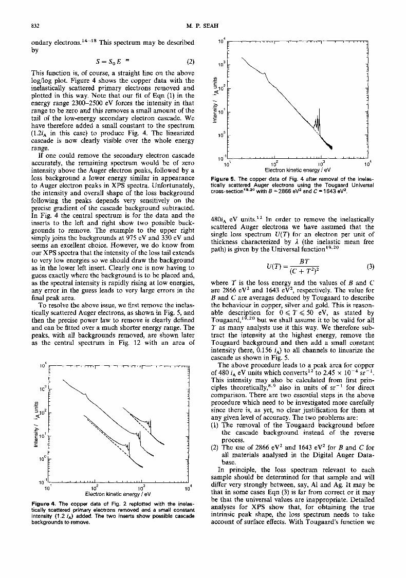
S = So E-” (2) This function is, of course, a straight line on the above log/log plot. Figure 4 shows the copper data with the inelastically scattered primary electrons removed and plotted in this way. Note that our fit of Eqn (1) in the energy range 2300-2500 eV forces the intensity in that range to be zero and this removes a small amount of the tail of the low-energy secondary electron cascade. We have therefore added a small constant to the spectrum (1.2iA in this case) to produce Fig. 4. The linearized cascade is now clearly visible over the whole energy range.

If one could remove the secondary electron cascade accurately, the remaining spectrum would be of zero intensity above the Auger electron peaks, followed by a loss background a lower energy similar in appearance to Auger electron peaks in XPS spectra. Unfortunately, the intensity and overall shape of the loss background following the peaks depends very sensitively on the precise gradient of the cascade background subtracted. In Fig. 4 the central spectrum is for the data and the inserts to the left and right show two possible backgrounds to remove. The example to the upper right simply joins the backgrounds at 975 eV and 330 eV and seems an excellent choice. However, we do know from our XPS spectra that the intensity of the loss tail extends to very low energies so we should draw the background as in the lower left insert. Clearly one is now having to guess exactly where the background is to be placed and, as the spectral intensity is rapidly rising at low energies, any error in the guess leads to very large errors in the final peak area.

To resolve the above issue, we first remove the inelastically scattered Auger electrons, as shown in Fig. 5, and then the precise power law to remove is clearly defined and can be fitted over a much shorter energy range. The peaks, with all backgrounds removed, are shown later as the central spectrum in Fig. 12 with an area of

look

I d I I

10’ 1 o2 1 o3 1 o4 Electron kinetic energy / eV

Figure 4. The copper data of Fig. 2 replotted with the inelastically scattered primary electrons removed and a small constant intensity (1.2 in) added. The two inserts show possible cascade backgrounds to remove.

104 I I

c 4

10-1 I I I 1 o1 1 o2 1 o3 1 o4

Electron kinetic energy I eV

Figure 5. The copper data of Fig. 4 after removal of the inelastically scattered Auger electrons using the Tougaard Universal cross-section’8*z0 with B = 2866 eVz and C = 1643 eV2.

480iA eV units.I2 In order to remove the inelastically scattered Auger electrons we have assumed that the single loss spectrum U(T) for an electron per unit of thickness characterized by Iz (the inelastic mean free path) is given by the Universal f ~ n c t i o n ~ ~ ~ ~ ~

BT (C + T2)2

U ( T ) = (3)

where T is the loss energy and the values of B and C are 2866 eV2 and 1643 eV2, respectively. The value for B and C are averages deduced by Tougaard to describe the behaviour in copper, silver and gold. This is reasonable description for 0 < T < 50 eV, as stated by T o ~ g a a r d , ’ ~ ’ ~ ~ but we shall assume it to be valid for all T as many analysts use it this way. We therefore subtract the intensity at the highest energy, remove the Tougaard background and then add a small constant intensity (here, 0.156 iA) to all channels to linearize the cascade as shown in Fig. 5.

The above procedure leads to a peak area for copper of 480 i, eV units which converts” to 2.45 x sr-l. This intensity may also be calculated from first prin- ciples theoreti~ally,~.~ also in units of sr-I for direct comparison. There are two essential steps in the above procedure which need to be investigated more carefully since there is, as yet, no clear justification for them at any given level of accuracy. The two problems are: (1) The removal of the Tougaard background before

the cascade background instead of the reverse process.

(2) The use of 2866 eV2 and 1643 eV2 for B and C for all materials analysed in the Digital Auger Data- base.

In principle, the loss spectrum relevant to each sample should be determined for that sample and will differ very strongly between, say, A1 and Ag. It may be that in some cases Eqn (3) is far from correct or it may be that the universal values are inappropriate. Detailed analyses for XPS show that, for obtaining the true intrinsic peak shape, the loss spectrum needs to take account of surface effects. With Tougaard‘s function we


do not have control over such details of the loss spectrum but we do have control over the intensity of the loss and the average loss energy through the values chosen for B and C. If the precise values of B and C are significant we shall have to find an automatic method of deducing B and C or practical analysts are faced with an impossible situation of developing some other procedure to define the relevant values, which may then lead to sample-to-sample inconsistencies. Of course, it would be best to remove the correct loss spectrum for each sample, where such a loss spectrum is available, but that would only apply to a few elements and selected pure compounds. In the eventual use of the Digital Auger Database, the intensities will be compared with those for an industrial sample of unknown loss spectrum and then, at the present time we see, as a practical option, the use of Eqn (3) with, hopefully, defined values of B and C.

In this paper, therefore, we study firstly the effect of removal of the Tougaard background for synthetic peaks on a cascade background to show the extent of error involved in item (1) above. Secondly, we analyse the effect of varying the values of B, and C, in the sample when Tougaard background parameters B, and C, are fixed at the universal values, and vice versa to show how the errors arising from unmatched B and C values may be minimized. In the sections that follow the subscripts S and T will be used to distinguish Tougaard values used to generate synthetic sample spectra and those used to define a background removal function, respectively.

THEORY

It is worth, first, evaluating some of the Tougaard parameters. For an infinitely thick homogeneous medium with no elastic scattering and where the excita- tion is homogeneous with depth, the integral of U(T) over all T should be unity. Tougaard‘s work with elastic scattering” gives

F(E) = j ( E ) - - ATL r K ( E - Elj(E) d E (4)

where F(E) is the primary peak structure we seek, j ( E ) is the measured spectrum after correction for the instru- ment transmission function, L is -2-5 times the trans- port mean free path for elastic scattering, &, and K(E’ - E ) is the probability that the electrons lose energy E - E (equals T ) at energy E per unit energy loss and unit path travelled in the solid. For use with the Universal function, Tougaard sets K(T) equal to

U( T) and

(5)

where C retains the value noted earlier but B , is now a fitting parameter set so that F(E) = 0 in a wide energy range below the peak energy. In the present work, we shall not fit B, in this way but substitute B , and C by trial values B, and CT .

Now

so that the intensity of the first loss spectrum is (B,/2CT) times that of the zero loss, F(E), and so on. Without elastic scattering, BT/~CT should be unity. From Eqn (5) it is approximately A L / ( A + L). Calculations for many elements” show that the ratio of elastic and inelastic scattering is not very dependent on atomic number and so a value for BT/2C, of 0.825 k 0.020 would be valid for all elements if L = 2Atr,” rising to 0.922 k 0.020 if L = 5At,.z3 The Universal cross section with BT = 2866 eV2 and C, = 1643 eVz exhibits a value of BT/~CT = 0.872, which lies in the middle of this range. Analyses for Cu and Au give B/2C values of 0.916 and 0.924, re~pectively.’~ In our later tests it will be assumed that BT/2C, may have values in the range 0.83-0.95.

A second parameter of interest in the Tougaard Uni- versal function is the centroid of the loss function, given by

Thus, within the range of BT/~CT given above we may expect that CT could range from 820 to 2500 eVZ, leading to E values ranging from 45 to 80 eV. These two considerations provide a useful computational range for B, and C, values, as shown in Table I.

First we generate a synthetic loss spectrum for j(E) based on a delta function of lo5 counts at 1000 eV kinetic energy, followed by all of the multiple losses based on Eqn (3) for various values of B, and C,. Ini- tially, to save time, we started with Vegh’s analytical form of the multiple lossesz5 but found that this was only a reasonable approximation to the required function for B, = 2866 eV2 and C, = 1643 eV2. For other values the approximation was poor. We have, therefore, generated the synthetic loss spectrum by summing up to 50 numerical convolutions using Fourier transforms

Table 1. The BT values for Tougaard background removal for selected values of &/2C, and of C,

4/2C, CT 0.83 0.85 0.872 0.83 0.91 0.93 0.95

821.5 1363.69 1396.55 1433 1462.27 1495.1 3 1 527.99 1560.85 1643 2727.38 2793.1 2866 2924.54 2990.26 3055.98 31 21.70 2464.5 4091.07 41 89.65 4299 4386.81 4485.39 4583.97 4682.55

834 M. P. SEAH

18001 I I I I I I

I I I I I I 200 400 600 800 1000 -200;

kinetic energy I eV

I I I 1 I I

G 0

\"I I - -50-

C m c 0

Q &-loo-

? 3 8-150-

-200 -

I I I I I I 200 400 600 800 1000

-250' 0

kinetic energy I eV

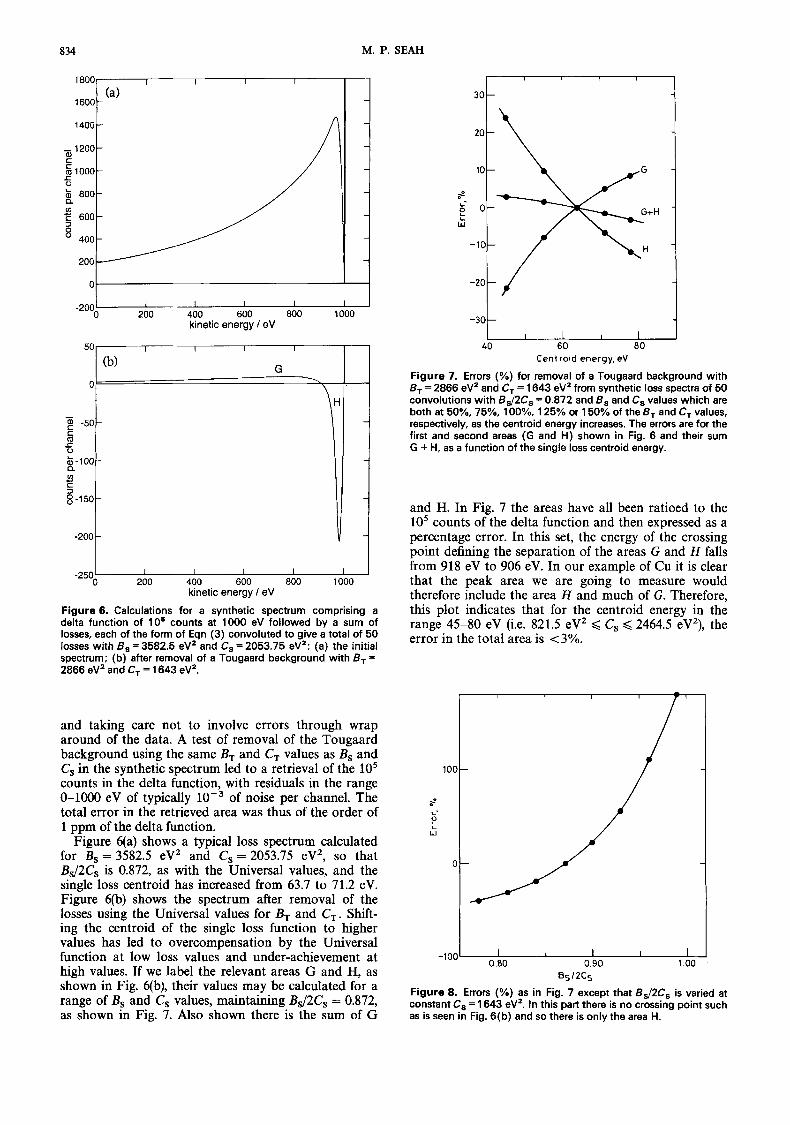
Figure 6. Calculations for a synthetic spectrum comprising a delta function of l o 6 counts at 1000 eV followed by a sum of losses, each of the form of Eqn (3) convoluted to give a total of 50 losses with B , = 3582.5 eV2 and C, = 2053.75 eV2: (a) the initial spectrum; (b) after removal of a Tougaard background with B, = 2866 eV2 and C, = 1643 eV2.

and taking care not to involve errors through wrap around of the data. A test of removal of the Tougaard background using the same BT and CT values as B, and C, in the synthetic spectrum led to a retrieval of the lo5 counts in the delta function, with residuals in the range 0-lo00 eV of typically lop3 of noise per channel. The total error in the retrieved area was thus of the order of 1 ppm of the delta function.

Figure qa) shows a typical loss spectrum calculated for B, = 3582.5 eV2 and C,= 2053.75 eV2, so that Bd2C, is 0.872, as with the Universal values, and the single loss centroid has increased from 63.7 to 71.2 eV. Figure qb) shows the spectrum after removal of the losses using the Universal values for BT and C,. Shift- ing the centroid of the single loss function to higher values has led to overcompensation by the Universal function at low loss values and under-achievement at high values. If we label the relevant areas G and H, as shown in Fig. 6(b), their values may be calculated for a range of B, and C, values, maintaining B$2C, = 0.872, as shown in Fig. 7. Also shown there is the sum of G

40 60 80 Centroid energy, eV

Figure 7. Errors (%) for removal of a Tougaard background with B, = 2866 eV2 and C, = 1643 eV2 from synthetic loss spectra of 50 convolutions with BJ2Cs = 0.872 and B, and C, values which are both at 50%, 75%, 1 OO%, 1 25% or 150% of the B, and C, values, respectively, as the centroid energy increases. The errors are for the first and second areas (G and H) shown in Fig. 6 and their sum G + H, as a function of the single loss centroid energy.

and H. In Fig. 7 the areas have all been ratioed to the lo5 counts of the delta function and then expressed as a percentage error. In this set, the energy of the crossing point defining the separation of the areas G and H falls from 918 eV to 906 eV. In our example of Cu it is clear that the peak area we are going to measure would therefore include the area H and much of G. Therefore, this plot indicates that for the centroid energy in the range 45-80 eV (i.e. 821.5 eV2 < C, < 2464.5 eV2), the error in the total area is < 3%.

100 ! s P i

W

0 80 0.90 1.00 -100

BS12CS

Figure 8. Errors (%) as in Fig. 7 except that B$2Cs is varied at constant C, = 1643 eV2. In this part there is no crossing point such as is seen in Fig. 6(b) and so there is only the area H.


' O ' q

loot ' 8 1 t 1 ' 1 ' I 1

10' 1 o2 1 o3 1 o4 kinetic energy / eV

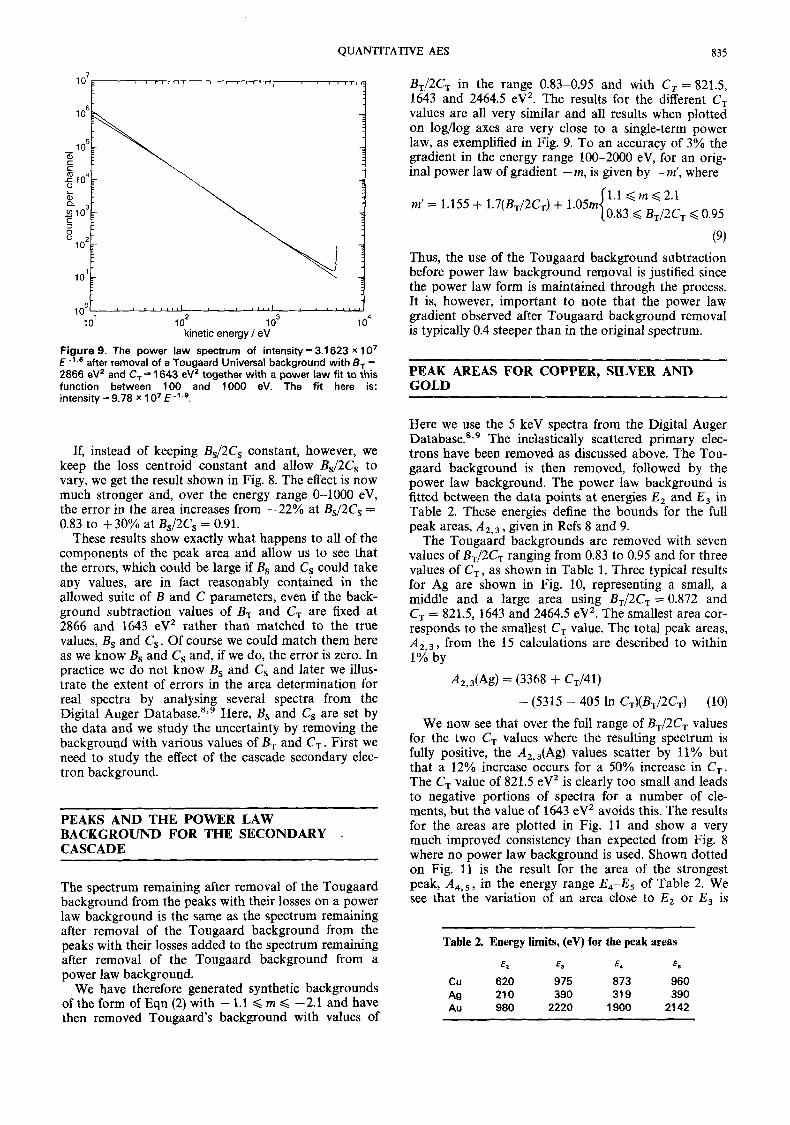
Figure 9. The power law spectrum of intensity = 3.1 623 x 10' €-'.' after removal of a Tougaard Universal background with B, = 2866 eV2 and C, = 1643 eVZ together with a power law fit to this function between 100 and 1000 eV. The fit here is: intensity = 9.78 x 1 O7 E-'.'.

If, instead of keeping B,/2Cs constant, however, we keep the loss centroid constant and allow B,/2Cs to vary, we get the result shown in Fig. 8. The effect is now much stronger and, over the energy range 0-1000 eV, the error in the area increases from -22% at B,/2Cs = 0.83 to +30% at B,/2Cs = 0.91.

These results show exactly what happens to all of the components of the peak area and allow us to see that the errors, which could be large if B, and Cs could take any values, are in fact reasonably contained in the allowed suite of B and C parameters, even if the background subtraction values of BT and C, are fixed at 2866 and 1643 eV2 rather than matched to the true values, B, and Cs. Of course we could match them here as we know B, and C, and, if we do, the error is zero. In practice we do not know B, and C, and later we illus- trate the extent of errors in the area determination for real spectra by analysing several spectra from the Digital Auger Databa~e.~, ' Here, B, and C, are set by the data and we study the uncertainty by removing the background with various values of B, and C,. First we need to study the effect of the cascade secondary electron background.

PEAKS AND THE POWER LAW BACKGROUND FOR THE SECONDARY CASCADE

The spectrum remaining after removal of the Tougaard background from the peaks with their losses on a power law background is the same as the spectrum remaining after removal of the Tougaard background from the peaks with their losses added to the spectrum remaining after removal of the Tougaard background from a power law background.

We have therefore generated synthetic backgrounds of the form of Eqn (2) with - 1.1 < rn < -2.1 and have then removed Tougaard's background with values of

BT/2CT in the range 0.83-0.95 and with C, = 821.5, 1643 and 2464.5 eV2. The results for the different C, values are all very similar and all results when plotted on log/log axes are very close to a single-term power law, as exemplified in Fig. 9. To an accuracy of 3% the gradient in the energy range 100-2000 eV, for an original power law of gradient - m, is given by - m', where

(9) Thus, the use of the Tougaard background subtraction before power law background removal is justified since the power law form is maintained through the process. It is, however, important to note that the power law gradient observed after Tougaard background removal is typically 0.4 steeper than in the original spectrum.

PEAK AREAS FOR COPPER, SILVER AND GOLD

Here we use the 5 keV spectra from the Digital Auger Database.',' The inelastically scattered primary electrons have been removed as discussed above. The Tou- gaard background is then removed, followed by the power law background. The power law background is fitted between the data points at energies E , and E3 in Table 2. These energies define the bounds for the full peak areas, A2,3, given in Refs 8 and 9.

The Tougaard backgrounds are removed with seven values of B&C, ranging from 0.83 to 0.95 and for three values of C,, as shown in Table 1. Three typical results for Ag are shown in Fig. 10, representing a small, a middle and a large area using B&CT = 0.872 and CT = 821.5, 1643 and 2464.5 eV2. The smallest area cor- responds to the smallest C, value. The total peak areas, A 2 , 3 , from the 15 calculations are described to within 1% by

A2,3(Ag) = (3368 + C,/41) - (5315 - 405 In CT)(B,/~C,) (10)

We now see that over the full range of BT/& values for the two C, values where the resulting spectrum is fully positive, the A2,:,(Ag) values scatter by 11% but that a 12% increase occurs for a 50% increase in C,. The C , value of 821.5 eV2 is clearly too small and leads to negative portions of spectra for a number of elements, but the value of 1643 eV2 avoids this. The results for the areas are plotled in Fig. 11 and show a very much improved consistency than expected from Fig. 8 where no power law background is used. Shown dotted on Fig. 11 is the result for the area of the strongest peak, A4,5, in the energy range E,-E, of Table 2. We see that the variation of an area close to E 2 or E , is

Table 2. Energy limits, (eV) for the peak areas

€2 €3 E l E.

cu 620 975 873 960 Ag 21 0 390 31 9 390 AU 980 2220 1 900 21 42

836 M. P. SEAH

1500

1000- > 4

.J" I I I I I I I

-

-lo 150 200 250 300 350 400 Electron kinetic energy I eV

Figure 10. Auger electron spectra for the Ag MNN peaks with all backgrounds removed using BT/2C, = 0.872: the lowest spectrum uses C, - 821.5 eV', the middle spectrum uses C, = 1643 eV2 and the highest spectrum uses C, = 2464.5 eV2.

much reduced over the variation for the total area. The variation in A4,5 with BT/~CT is now only +2% but still an 8% increase in this area occurs for a 50% increase in C,. It is unlikely that these deviations can be reduced much further and so we expect an uncertainty of +8% in the absolute value of determination, arising from an assumption that B, = 2866 eV2 and CT = 1643 eV2,

The area of the M4, ,NN peak, A4, ,(Ag), is given by

A4,5(Ag) = (686 + C,/183)

- (1151 - 127 In cT)(BT/2cT) (11) Figure 12 shows the data comparable to Fig. 10 but for the Cu spectra. Figure 13 complements Fig. 11, and the

CT.eV2

2464.5

1643

821.5

0- 0.8 0.9

BY/2CT

Figure 11. The silver Auger electron peak areas after all backgrounds have been removed for three C, values: (-) AZs3 (Ag) ; (- - -1 ( A d .

Q .- . .- 2.6 fA C a, - 2 4

2

0

600 650 700 750 800 850 900 950 Electron kinetic energy I eV

10

Figure 12. As Fig. 10 but for the Cu LMM peaks.

areas of the peaks are given by

A,,,(Cu) = 1220 - (2041 - 162 In CT)(BT,/2CT) (12)

(13) A4,5(Cu) = 257 - (479 - 53 In CT)(B,/2CT)

The variations of A2,3(C~) and A4,,(Cu) are essentially similar to those for Ag but with a major improvement arising from selection of the highest energy peak.

Finally, in Fig. 14 we show the set of spectra for Au, comparable to Figs 10 and 12 for Cu and Ag, respectively, with the areas plotted in Fig. 15. Since much of the problem of peak areas is clearly governed by the precision of the background removal, we would expect the problem to scale with the the relative width of the spectral region and with the relative intensities of the peaks above the background. The relative widths of the energy ranges are given by the ratio E 3 / E , , which increases in the order Cu, Ag and Au. The Cu and Ag

600

CT ,eV*

2464.5

1643 .

821.5


1 . 6 6

1.2 '.i

I I I I I

1000 1200 1400 1600 1800 2000 2200 -0.2' I

Electron kinetic energy I eV

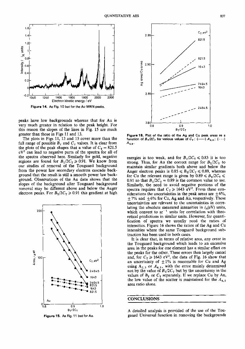
Figure 14. As Fig. 10 but for the Au MNN peaks.

peaks have low backgrounds whereas that for Au is very much greater in relation to the peak height. For this reason the slopes of the lines in Fig. 15 are much greater than those in Figs 11 and 13.

The plots in Figs 11, 13 and 15 cover more than the full range of possible B, and C , values. It is clear from the plots of the peak shapes that a value of CT = 821.5 eVZ can lead to negative parts of the spectra for all of the spectra observed here. Similarly for gold, negative regions are found for B&?CT 2 0.91. We know from our studies of removal of the Tougaard background from the power law secondary electron cascade background that the result is still a smooth power law background. Observations of the Au data shows that the slopes of the background after Tougaard background removal may be different above and below the Auger electron peaks. For BT/2C, 2 0.91 this gradient at high

I

t

CT. ev2

2 4 6 4 5

1643

2664.5 821.5 1643 821.5

Figure 15. As Fig. 11 but for Au.

I 1

0.8 0.9 1 .o B T I 2 C T

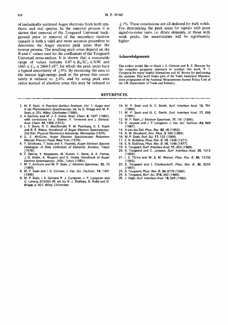
Figure 16. Plot of the ratio of the Ag and Cu peak areas as a function of B1/2C1 for various values of C, : (-) A2,3 ; (- - -) 4 . 6 .

energies is too weak, and for BT/2C, < 0.83 it is too strong. Thus, for Au the correct range for B T / ~ C T to maintain similar gradients both above and below the Auger electron peaks is 0.85 < B,/2CT < 0.89, whereas for Cu the relevant range is given by 0.89 < < 0.91 so that B T / ~ C T = 0.89 is the common value to use. Similarly, the need to avoid negative portions of the spectra requires that C; 1643 eVZ. From these considerations the uncertainties in the peak areas are & 6%, f 7% and +_ 6% for Cu, Ag and Au, respectively. These uncertainties are relevant to the uncertainties in corre- lating the absolute measured intensities in i,(eV) units, which convert to sr-l units for correlation with theoretical predictions in sirnilar units. However, for quanti- fication of spectra we usually need the ratios of intensities. Figure 16 shows the ratios of the Ag and Cu intensities where the sa,me Tougaard background subtraction has been used in both cases.

It is clear that, in terms of relative area, any error in the Tougaard background which leads to an excessive area in the peaks for one element has a similar effect on the peaks for the other. These errors then largely cancel and, for CT 2 1643 eV2, the data of Fig. 16 show that an uncertainty of *1% is reasonable for Cu and Ag using A2,3 or ,44,s, with the error mainly determined not by the value of BT/2CT but by the uncertainty in the values of BT or C , separately. If we replace Cu by Au, the low value of the scatter is maintained for the A4,s area ratio alone.

CONCLUSIONS

A detailed analysis is provided of the use of the Tou- gaard Universal function in removing the backgrounds

838 M. P. SEAH

of inelastically scattered Auger electrons from both synthetic and real spectra. In the removal process it is shown that removal of the Tougaard Universal background prior to removal of the secondary electron cascade is both a valid and more accurate procedure to determine the Auger electron peak areas than the reverse process. The resulting peak areas depend on the B and C values used for the coefftcients of the Tougaard Universal cross-section. It is shown that a reasonable range of values includes 0.87 < BT/2C, < 0.90 and 1643 < C, < 2464.5 eV2, for which the peak areas have a typical uncertainty of +6%. By restricting the area to the intense high-energy peak in the group this uncertainty is reduced to &4%, and by using peak area ratios instead of absolute areas this may be reduced to

& 1%. These conclusions are all deduced for bulk solids. For determining the peak areas for signals with poor signal-to-noise ratio, i.e. dilute elements, or those with weak peaks, the uncertainties will be significantly higher.

Acknowledgements

The author would l ike to thank I. S. GiImore and R. E. Shawyer for the computer programs necessary to conduct this work, P. J. Cumpson for many helpful discussions and M. Brown for performing the analyses. T h i s work forms part of the Valid Analytical Measure- ment programme of the National Measurement System Policy Unit of the UK Department of Trade and Industry.

REFERENCES

1, M. P. Seah, in Practical Surface Analysis, Vol. 1 : Auger and X-ray Photoelectron Spectroscopy, ed. by 0. Briggs and M. P. Seah, p. 201. Wiley, Chichester (1 990).

2. A Savitzky and M. J. E. Golay, Anal. Chem. 6, 1627 (1 964), with corrections by J. Steiner, Y. Termonia and J. Deltour, Anal. Chem. 44,1906 (1 972).

3. L. E. Davis, N. C. MacDonald, P. W. Palmberg, G. E. Riach and R. E. Weber, Handbook of Auger Electron Spectroscopy, 2nd Edn. Physical Electronics Industries, Minnesota (1 976).

4. G. E. McGuire, Auger Electron Spectroscopy Reference Manual. Plenum Press, New York (1 979).

5. Y. Shiokawa, T. lsida and Y. Hayashi, Auger Electron Spectra Catalogue4 Data Collection of Elements. Aneleva, Tokyo

6. T. Sekine, Y. Nagasawa, M. Kudoh, Y. Sakai, A. S. Parkes, J. D. Geller, A. Mogami and K. Hirata, Handbook of Auger Electron Spectroscopy. JEOL, Tokyo (1 982).

7. M. T. Anthony and M. P. Seah, J. Electron Spectrosc. 32, 73 (1983).

8. M. P. Seah and I. S. Gilmore, J. Vac. Sci. Technol., 14, 1401 (1 996).

9. M. P. Seah, I. S. Gilmore, P. J. Cumpson, J. P. Langeron and G. Lorang, ECASlA 95. ed. by H. J. Mathieu, B. Reihl and D. Briggs, p. 607, Wiley, Chichester.

(1979).

10. M. P. Seah and G. C. Smith, Surf. Interface Anal. 15, 751

11. M. P. Seah and G. C. Smith, Surf. Interface Anal. 17, 855

1 2. M. P. Seah, J. Electron Spectrosc. 71,191 (1 995). 13. D. Jousset and J. P. Langeron, J. Vac. Sci. Technol. A5, 989

14. A van der Ziel, Phys. Rev. 92, 35 (1 953). 15. H. W. Streitwolf, Ann. Phys. 3, 183 (1 959). 16. M. P. Seah,Surf. Sci. 17,132 (1969). 17. E. N. Sickafus, Phys. Rev. B, 16,1436 (1 977). 18. E. N. Sickfaus, Phys. Rev. B, 16, 1448 (1977). 19. S. Tougaard, Surf. lnterface Anal. 11,453 (1 988). 20. S. Tougaard and C. Jansson, Surf. lnterface Anal. 20, 1013

21. I. S. Tilinin and W. S. M. Werner, Phys. Rev. B, 46, 13739

22. S. Tougaard and 1. Chorkendorff, Phys. Rev. 8, 35, 6570

23. S. Tougaard, Phys. Rev. B, 34,6779 (1 986). 24. S. Tougaard, Surf. Sci. 21 6,343 (1 989). 25. J. Vegh,Surf. Interface Anal. 18, 545 (1992).

(1 990).

(1991).

(1 987).

(1993).

(1 992).

(1 987).

Quantitative AES IV: Accuracy of the Numerical Evaluation of Peak Areas in AES using the Universal...

Documents

Transcript of Quantitative AES IV: Accuracy of the Numerical Evaluation of Peak Areas in AES using the Universal...