Quantifying Reciprocity in Large Weighted Communication Networks

Quantifying Reciprocity in Large WeightedCommunication Networks

Leman Akoglu1,3, Pedro O.S. Vaz de Melo2,3, and Christos Faloutsos1,3

1 Carnegie Mellon University, School of Computer Science2 Universidade Federal de Minas Gerais

3 iLab, Heinz College4 [email protected], [email protected], [email protected]

Abstract. If a friend called you 50 times last month, how many times did youcall him back? Does the answer change if we ask about SMS, or e-mails? Wewant to quantify reciprocity between individuals in weighted networks, and wewant to discover whether it depends on their topological features (like degree, ornumber of common neighbors). Here we answer these questions, by studying thecall- and SMS records of millions of mobile phone users from a large city, withmore than 0.5 billion phone calls and 60 million SMSs, exchanged over a periodof six months. Our main contributions are: (1) We propose a novel distribution,the Triple Power Law (3PL), that fits the reciprocity behavior of all 3 datasetswe study, with a better fit than older competitors, (2) 3PL is parsimonious; it hasonly three parameters and thus avoids over-fitting, (3) 3PL can spot anomalies,and we report the most surprising ones, in our real networks, (4) We observe thatthe degree of reciprocity between users is correlated with their local topologi-cal features; reciprocity is higher among mutual users with larger local networkoverlap and greater degree similarity.

1 Introduction

One of the important aspects in human relations is the reciprocity, a.k.a. mutuality. Reci-procity can be defined as the tendency towards forming mutual connections with oneanother by returning similar acts, such as email and phone calls. In a highly reciprocalrelationship both parties share equal interest in keeping up their relationship, while in arelationship with low reciprocity, one person is much more active than the other.

It is important to understand the factors that play role in the formation of reciprocityas there exists evidence that reciprocal relationships are highly probable to persist in thefuture [6]. Also, [18] shows that reciprocity related behaviors provide good features forranking and classification based methods for trust prediction. Reciprocity plays otherimportant roles in social and communication networks. For example, if the network sup-ports a propagation process, such as spreading of viruses in email networks or spreadingof information and ideas in social networks, then the presence of mutual links clearlyspeeds up the propagation. Non-existence of reciprocal links can also reveal unwantedcalls and emails in spam detection.

Despite its importance, reciprocity has remained an under-explored dynamic in net-works. Most work in network science and social network analysis focus on node leveldegree distributions [5, 10, 14], communities [20, 22, 19], and triadic relations, such as

2 Leman Akoglu, Pedro O.S. Vaz de Melo, and Christos Faloutsos

clustering coefficients and triangle closures [12]. The study of dyadic relations [26] andthe related bivariate distributions they introduce is, however, mostly overlooked, andthus is the focus of this paper. Our motivation is grouped into two topics:

M1. Modeling bivariate distributions in real data: Two vital components of un-derstanding data at hand are studying the simple distributions in it and visualizingit [27]. The study of reciprocity introduces bivariate distributions, such as the distri-bution Pr(wij , wji) of edge weights on mutual edges, where association between twoquantitative variables needs to be explored. A vast majority of existing work focus onunivariate distributions in real data such as power-laws [8], log-normals [4], and mostrecently DPLNs [21], however the study of multivariate distributions has limited focus.

In addition, visualization of multivariate data in 2D is hard and often misleadingdue to issues regarding over-plotting. More importantly, mere visualization does notprovide a compact data representation as opposed to data modeling. Summarization viaaggregate functions such as the average or the median loses a lot of information and isalso not representative, especially for skewed distributions as found in real data.

Models, on the other hand, provide compact data representations by capturing thepatterns in the data, and are ideal tools for applications like data compression andanomaly detection.

M2. A weighted approach to reciprocity: Traditional work [11] usually study reci-procity on directed, unweighted networks as a global feature which is quantified as theratio of the number of mutual links pointing in both directions to the total number oflinks. Defining reciprocity in such an unweighted fashion, however, prevents under-standing the degree of reciprocity between mutual dyads. In a weighted network, eventhough two nodes might have mutual links between them, the skewness and the magni-tude of the weights associated with these links would contain more information abouthow much reciprocity is really there between these nodes. For example, in a phone callnetwork the reciprocity between a mutual dyad where the parties make 80%-20% oftheir calls respectively is certainly different than that of a mutual dyad with 50%-50%share of their calls. In short, edge weights are crucial to study reciprocity as a propertyof each dyad rather than as a global feature of the entire network and give more insightinto the level of mutuality.

In this paper, we analyze phone call and SMS records of 1.87 million mobile phoneusers from a large city collected over six months. The data consists of over half a billionphone calls and more than 60 million SMSs exchanged. Our contributions are:

1. We observe similar bivariate distributions Pr(wij , wji) of mutual edge weights inthe communication networks we study. We propose the Triple Power Law (3PL)function to model this observed pattern and show that 3PL fits the real data withmillions of points very well. We statistically demonstrate that 3PL provides betterfits than the well-known Bivariate Pareto and Bivariate Yule distributions. We alsouse 3PL to spot anomalies, such as a pair of users with low mutuality where one ofthe parties makes 99% of the calls during the entire working hours, non-stop.

2. We use weighted measures of reciprocity in order to quantify the degree of recip-rocal relations and study the correlations between reciprocity and local topologicalfeatures among user pairs. Our results suggest that mutual users with larger localnetwork overlap and higher degree similarity exhibit greater reciprocity.

Quantifying Reciprocity in Large Weighted Communication Networks 3

2 Related Work

Bivariate Distributions in Real Data: A vast majority of existing work focus on uni-variate distributions in real data such as power-laws, Pareto distributions and so on [17].For example, the degree distribution has been found to obey a power-law in many realgraphs such as the Internet Autonomous Systems graph [10], the WWW link graph [1],and others [5, 7]. Additional power laws seem to govern the popularity of posts in cita-tion networks, which drops over time, with power law exponent of -1 for paper citationsand -1.5 for blog posts [14].

A recent comprehensive study [8] on power-law distributions in empirical datashows that while power-laws exist in many graphs, deviations from a pure power-laware also observed. Those deviations usually appear in the form of exponential cut-offsand log-normals. Similar deviations were also observed in [2] where the electric power-grid graph in a specific region in California as well as airport networks were found toexhibit power-law distributions with exponential cut-offs.

Other deviations from power-laws continue. Discrete Gaussian Exponential (DGX) [4]was shown to provide good fits to distributions in a variety of real world data sets suchas the Internet click-stream data and usage data from a mobile phone operator. Most re-cently, [21] studied several phone call networks and proposed a new distribution calledthe Double Pareto Log-Normal (DPLN) that was used to separately model the per-usernumber of call partners, number of calls and number of minutes. Other related work onexplaining and modeling the behaviour of phone network users include [6, 9, 16, 23].

While univariate distributions are used to model the distribution of a specific quan-tity x, for example the number of calls of users, bivariate distributions are used to modelthe association and co-variation between two quantitative variables x1 and x2. Associ-ation is based on how two variables simultaneously change together, for example thetotal number of calls with respect to the number of call partners of users.

Unlike univariate distributions, the multivariate distributions have mostly been stud-ied theoretically in mathematics and statistics [3]. On the other hand, analysis of espe-cially skewed multivariate distributions in real data has attracted much less focus. Ex-isting work includes [28], which uses the bivariate log-normal distribution to describethe joint distributions of flood peaks and volumes, as well as flood volumes and dura-tions. Also, [15] studies the drought in the state of Nebraska and models the durationand severity, proportion and inter-arrival time, and duration and magnitude of droughtwith bivariate Pareto distributions.Reciprocity in Unweighted Networks: Previous studies usually consider reciprocity asa global metric of a given directed network where reciprocity is quantified as r=L

↔

L , theratio of the number of mutual links L↔ pointing in both directions to the total numberof links L. By definition, r=1 for a purely bidirectional network (e.g. collaborationnetworks) and r=0 for a purely unidirectional network (e.g. citation networks).

There are two issues with this definition. First, it depends on the density of the net-work; reciprocity is larger in a network with larger link density. Second, this definitiontreats the graph as unweighted, and thus fails to quantify the degree of reciprocity be-tween mutual dyads. [11] combines this classical definition with the network densityinto a single measure which tackles the first problem, however the new measure still re-mains a global, unweighted metric and does not allow to study the degree of reciprocity.


3 Data Description

In this work, we study anonymous mobile communication records of millions of userscollected over a period of six months, December 1, 2007 through May 31, 2008. Thedata set contains both phone call and SMS interactions.

From the whole six months’ of activity, we build three networks, CALL-N, CALL-D and SMS, in which nodes represent users and directed edges represent phone calland SMS interactions between these users. CALL-N is a who-calls-whom networkwith edge weights denoting (1) total number of phone calls, CALL-D is the samewho-calls-whom network with edge weights denoting (2) total duration of phone calls(aggregated in minutes), and SMS is a who-texts-whom network with edge weightsdenoting (3) total number of SMSs. Table 1 gives the data statistics. Global unweightedreciprocity is r=0.84 for CALL, and r=0.24 for SMS.

Table 1. Data statistics. The number of nodes N , the number of directed edges E, and the totalweight W in the mutual and non-mutual CALL and SMS networks.

Network N E WN WD(min) Network N E WSMS

CALL 1,87M 49,50M 483,7M 915x106 SMS 1,87M 8,80M 60,5MCALL(mutual) 1,75M 41,84M 468,7M 885x106 SMS(mutual) 0,58M 2,10M 46,6M

4 Proposed Model: 3PL

Given a network of users with mutual, weighted edges between them, say CALL-N,and given two users i and j in the network, is there a relation between the number ofcalls i makes to j (wij) and the number of calls j makes to i (wji)? In this section, wewant to understand the association between the weights on the reciprocal edges in hu-man communication networks and study their distribution Pr(wij , wji) across mutualdyads. Since we study the pair-wise joint distribution, the order of the weights do notmatter. Thus, to ease notation, we will denote the smaller of these weights as nST (forweight from Silent-to-Talkative) and the larger as nTS , and will study Pr(nST , nTS).

Figure 1(top-row) shows the weights nTS versus nST for all the reciprocal edges in(from left to right) CALL-N, CALL-D, and SMS. Each dot in the plots correspondsto a pair of mutual edges. Since there could be several pairs with the same (nST , nTS)weights, the regular scatter plot of the reciprocal edge weights would result in over-plotting. Therefore, in order to make the densities of the regions clear, we show theheatmap of the scatter plots where colors represent the magnitude of volume (red meanshigh volume and blue means low volume).

In Figure 1, we observe that most of the points are concentrated (1) around the originand (2) along the diagonal for all three networks. Concentration around the origin, forexample in CALL-N, suggests that the vast majority of people make only a few phonecalls with nST , nTS < 10, and much fewer people make many phone calls, whichpoints to skewness. In addition, concentration along the diagonal indicates that mutualpeople call each other mostly in a balanced fashion with nST ≈ nTS . Notice thatsimilar arguments hold for CALL-D and SMS.

Even though heatmaps reveal similar patterns in all the three networks, mere visual-ization does not provide compact representations for our data. One way to go around this


100

101

102

103

100

101

102

103

104

nST

n TS

5

10

15

20

100

101

102

103

104

100

101

102

103

104

nST

n TS

0

5

10

15

20

100

101

103

102

104

100

101

102

103

104

nST

nT

S

2

4

6

8

10

12

14

16

100

105

101

102

103

104

100

101

102

103

104

105

nST

n TS (

aver

age)

0.98279x + (0.14191) = y

100

105

101

102

103

104

100

101

102

103

104

105

nST

n TS (a

vera

ge)

0.97373x + (0.19404) = y

100

105

101

102

103

104

100

101

102

103

104

105

nST

n TS (a

vera

ge)

0.77552x + (0.81978) = y

(a) CALL-N (b) CALL-D (c) SMS

Fig. 1. (top-row) Scatter plot heatmaps: total weight nST (Silent to Talkative) vs the reverse, nTS ,in log scales. Visualization by scatter plots suffers from over-plotting. Heatmaps color-code denseregions but do not have compact representations or formulas. Figures are best viewed in color;red points represent denser regions. The counts are in log2 scale. (bottom-row) Aggregation byaverage: summarization and data aggregation, e.g. averaging, loses a lot of information.

issue is to do data summarization. For example, Figure 1(bottom-row) shows how nTSchanges with nST on average. The least square fit of the data points in log-log scalesthen provides a mathematical representation of the data. Data summarization by meansof an aggregate function such as the average, however, loses a lot of information aboutthe actual distribution: in our example, the slope of the least square fit in CALL-N isclose to 1, which suggests that nTS is equal to nST on average, and does not provideany information for the deviations. This issue arises mostly because aggregation by theaverage is not a good representative, especially for skewed distributions.

Given our observation that the distribution of reciprocal edge weights (nST , nTS)follows a similar pattern across all three networks, how can we model the observeddistributions? Since neither visualization nor aggregation qualify for compact data rep-resentation, we propose to formulate the distributions with the following bivariate func-tional form Pr(nST , nTS), which we call the Triple Power-Law (3PL) function.

Proposed Model 1 (Triple Power-Law (3PL)) In human communication networks, thedistribution Pr(nST , nTS) of mutual edge weights nST and nTS (nST being the smaller)follows a Triple Power-Law in the following form

Pr(nST , nTS ;α, β, γ) ∝n−αST n

−βTS(nTS − nST + 1)−γ

Z(α, β, γ), α > 0, β > 0, γ > 0, and

nTS ≥ nST > 0, Z(α, β, γ) =∑MnST=1

∑MnTS=nST

n−αST n−βTS(nTS − nST + 1)−γ .

where Z is the normalization constant and M is a very large integer.

Next we elaborate on the intuition behind the exponents α, β and γ.


Intuition behind the β exponent: 3PL is the 2D extension of the “rich-get-richer”phenomenon; people who make many phone calls will continue making even more, andeven longer ones, leading to skewed, power-law-like distributions. The β exponent isthe skewness of the main component, the number nTS of phone-calls from ’talkative’ to’silent’. High β means more skewed distribution; β=0 is roughly uniform distribution.As we show in Figure 1, there are many people who make only a few (and short) phonecalls and only a few people who make many (and long) phone calls. Visually, the vastmajority of people who make only a few phone calls are represented with the highdensity (dark red) regions around the origin in all three networks.Intuition behind the α exponent: Similarly, this indicates the skewness for nST , thenumber of silent-to-talkative phone-calls. High value of α means high skewness, whileα close to zero means uniformity. Notice that α ≈ 0 for our real phone-call datasets(see Figure 2).Intuition behind the γ exponent: It captures the skewness in asymmetry. High γmeans that large asymmetries are improbable. This is the case in all our real datasets.For example, in addition to the origin in Figure 1(a), the regions along the diagonalalso have high densities. These regions correspond to mutual pairs with about equalinteraction in both directions. This suggests that humans tend to reciprocate their com-munications. 3PL also captures this observation; notice that the probability is higher fornTS close to nST and drops for larger inequality (nTS − nST ) as a power-law withexponent γ.

4.1 Comparison of 3PL to Competing Models

In this section, we compare our model with two well-known parametric distributionsfor skewed bivariate data, the Bivariate Pareto [13] and the Bivariate Yule [25]. Theirfunctional forms are given as two alternative competitor models as follows.

Competitor Model 1 (Bivariate Pareto)

fX1,X2(x1, x2) = k(k + 1)(ab)k+1(ax1 + bx2 + ab)−k−2, x1, x2, a, b, k > 0.

Competitor Model 2 (Bivariate Yule)

fX1,X2(x1, x2) =

ρ(2)(x1 + x2)!

(ρ+ 1)(x1+x2+2), x1, x2, ρ > 0;α(β) = Γ (α+β)/Γ (α), α > 0, β ∈ R.

We use maximum likelihood estimation to fit the parameters of each model foreach of our three networks. In Figure 2, we report the best-fit parameters as well asthe corresponding data log likelihood scores (the higher, the better). Notice that forCALL-N and CALL-D the 3PL achieves higher data likelihood than both BivariatePareto and Bivariate Yule. On the other hand, for SMS, the data likelihood scores of allthree models are about the same; with Bivariate Pareto giving a slightly higher score.

The simple sign of the difference between the log likelihoods (log likelihood ratioR), however, does not on its own show conclusively that one distribution is better thanthe other as it is subject to statistical fluctuation. If its true value over many indepen-dent data sets drawn from the same distribution is close to zero, then the fluctuations


can easily change its sign and thus the results of the comparison cannot be trusted. Inorder to make a firm judgement in favor of 3PL, we need to show that the differencebetween the log likelihoods is sufficiently large and that it could not be the result of achance fluctuation. To do so, we need to know the standard deviation σ onR, which weestimate from our data using the method proposed in [24].

Fig. 2. Maximum likelihood parameters estimatedfor 3PL, Bivariate Pareto and the Bivariate Yule anddata log-likelihoods obtained with the best-fit pa-rameters. We also give the normalized log likelihoodratios z and the corresponding p-values. A positive(and large) z value indicates that 3PL is favored overthe alternative. A small p-value confirms the signif-icance of the result. Notice that 3PL provides sig-nificantly better fits to CALL and is as good as itscompetitors for SMS.

CALL-N CALL-D SMSTriple Power Law (3PL)

α 1e-06 1e-06 0.8120β 2.0703 1.8670 1.5896γ 0.8204 0.9650 0.3005Loglikelihood -7.55e+07 -8.88e+07 -5.41e+06

Bivariate Paretok 0.7407 0.7657 0.7862a 0.2119 0.5723 0.7097b 10e+05 1.25e+04 0.7553Loglikelihood -7.77e+07 -9.26e+07 -5.39e+06z 803.73 975.75 -41.06p 0 0 0

Bivariate Yuleρ 1.11e-16 5.55e-17 1e-06Loglikelihood -8.59e+07 -10.00e+07 -5.41e+06z 2.14e+03 1.93e+03 1.49p 0 0 0.03

In Figure 2, we report thenormalized log likelihood ra-tio denoted by z = R/

√2nσ,

where n is the total number ofdata points (number of mutualedge pairs in our case). A pos-itive z value indicates that the3PL model is truly favored overthe alternative. We also showthe corresponding p-value, p =erfc(z), where erfc is the com-plementary Gaussian error func-tion. It gives an estimate of theprobability that we measured agiven value of R when the truevalue of R is close to zero (andthus cannot be trusted). There-fore, a small p value shows thatthe value ofR is unlikely to be achance result and its sign can betrusted.

Notice that the magnitude ofz for CALL-N and CALL-D isquite large, which makes the p-value zero and shows that 3PL isa significantly better fit for thosedata sets. On the other hand, zis relatively much smaller forSMS, therefore we concludethat 3PL provides as good of afit as its competitors for this data

set. Note that the number of mutual edge pairs n in SMS (≈1 million) is much smallercompared to that of the call networks (≈21 million) (Table 1). It is worth emphasizingthat difference, because the bivariate pattern of reciprocity might reveal itself better inlarger data sets, and it would be interesting to see whether 3PL provides a better fit forSMS when more data samples become available.

Next, we demonstrate also visually that 3PL provides a better fit to the real datathan its competitors. To this end, having estimated the model parameters for all threemodels, we generated synthetic data sets with the same number of samples as in eachof our networks. We show the corresponding plots for CALL-N in Figure 3 (a) for real


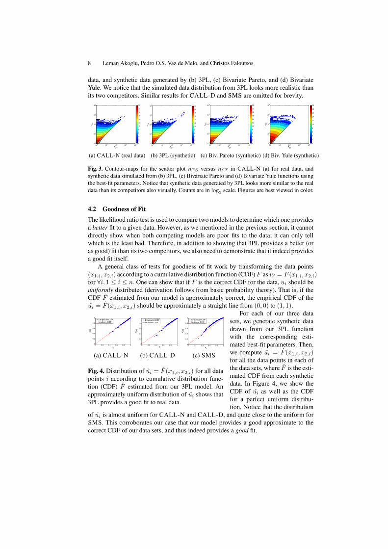
data, and synthetic data generated by (b) 3PL, (c) Bivariate Pareto, and (d) BivariateYule. We notice that the simulated data distribution from 3PL looks more realistic thanits two competitors. Similar results for CALL-D and SMS are omitted for brevity.

nST

nT

S

100

101

102

103

104

100

101

102

103

104

0

2

4

6

8

10

12

14

16

18

20

22

nST

nT

S

100

101

102

103

104

100

101

102

103

104

0

2

4

6

8

10

12

14

16

18

20

22

nST

nT

S

100

101

102

103

104

100

101

102

103

104

0

2

4

6

8

10

12

14

16

18

20

22

nST

nT

S

100

101

102

103

104

100

101

102

103

104

0

2

4

6

8

10

12

14

16

18

20

(a) CALL-N (real data) (b) 3PL (synthetic) (c) Biv. Pareto (synthetic) (d) Biv. Yule (synthetic)

Fig. 3. Contour-maps for the scatter plot nTS versus nST in CALL-N (a) for real data, andsynthetic data simulated from (b) 3PL, (c) Bivariate Pareto and (d) Bivariate Yule functions usingthe best-fit parameters. Notice that synthetic data generated by 3PL looks more similar to the realdata than its competitors also visually. Counts are in log2 scale. Figures are best viewed in color.

4.2 Goodness of Fit

The likelihood ratio test is used to compare two models to determine which one providesa better fit to a given data. However, as we mentioned in the previous section, it cannotdirectly show when both competing models are poor fits to the data; it can only tellwhich is the least bad. Therefore, in addition to showing that 3PL provides a better (oras good) fit than its two competitors, we also need to demonstrate that it indeed providesa good fit itself.

A general class of tests for goodness of fit work by transforming the data points(x1,i, x2,i) according to a cumulative distribution function (CDF)F as ui = F (x1,i, x2,i)for ∀i, 1 ≤ i ≤ n. One can show that if F is the correct CDF for the data, ui should beuniformly distributed (derivation follows from basic probability theory). That is, if theCDF F estimated from our model is approximately correct, the empirical CDF of theui = F (x1,i, x2,i) should be approximately a straight line from (0, 0) to (1, 1).

0 0.2 0.4 0.6 0.8 10

0.2

0.4

0.6

0.8

1

ui

F(u i)

Empirical CDFUniform CDF

0 0.2 0.4 0.6 0.8 10

0.2

0.4

0.6

0.8

1

ui

F(u i)


0 0.2 0.4 0.6 0.8 10

0.2

0.4

0.6

0.8

1

ui

F(u i)



Fig. 4. Distribution of ui = F (x1,i, x2,i) for all datapoints i according to cumulative distribution func-tion (CDF) F estimated from our 3PL model. Anapproximately uniform distribution of ui shows that3PL provides a good fit to real data.

For each of our three datasets, we generate synthetic datadrawn from our 3PL functionwith the corresponding esti-mated best-fit parameters. Then,we compute ui = F (x1,i, x2,i)for all the data points in each ofthe data sets, where F is the esti-mated CDF from each syntheticdata. In Figure 4, we show theCDF of ui as well as the CDFfor a perfect uniform distribu-tion. Notice that the distribution

of ui is almost uniform for CALL-N and CALL-D, and quite close to the uniform forSMS. This corroborates our case that our model provides a good approximate to thecorrect CDF of our data sets, and thus indeed provides a good fit.


4.3 3PL at work

There exist at least three levels at which we can make use of parametric statistical mod-els for real data: (1) as data summary: compact mathematical representation, data re-duction; (2) as simulators: generative tools for synthetic data; (3) in anomaly detection:probability density estimation.

100

105

101

102

103

10410

0

101

102

103

104

105

nST

n TS

<2h

>600h

Fig. 5. (a) Least likely 100 points by 3PL (shownwith triangles). (b) Local neighborhood of one mu-tual pair detected as an outlier (marked with circles).Edge thickness is proportional to edge weight.

In Figure 5(a), we show top100 pairs in CALL-D with low-est 3PL likelihood (marked withtriangles). Figure 5(b) shows thelocal neighborhood of one ofthe pairs, say A and B (markedwith circles in (a)). We noticelow mutuality; A initiated 99%of the calls in return to lessthan 2 hours total duration ofcalls B made. Further inspectionrevealed constant daily activityby A, including weekends, withabout 7 hours call duration perday on average, starting at around 9am in the morning until around 5-8pm in theevening. It is also surprising that all these calls are addressed to the same contact,B. While for privacy reasons, we cannot fully tell the scenario behind this behavior,this proves to be an interesting case for the service operator to further look into. Otherinteresting anomalous observations are omitted for brevity.

5 Reciprocity and Local Network Topology

Given that person i calls person j wij times and person j calls person i wji times, whatis the degree of reciprocity between them? In this section, we discuss several weightedmetrics that quantify reciprocity between a given mutual pair. Later, we study the rela-tionship between reciprocity among mutual pairs and their topological similarity.

5.1 Weighted reciprocity metrics

Three metrics we considered in this work to quantify the “similarity” or “balance”of weights wij and wji are (1) Ratio r =

min(wij ,wji)max(wij ,wji)

∈ [0, 1], (2) Coherence c =2√wijwji

(wij+wji)∈ [0, 1] (geometric mean divided by the arithmetic mean of the edge weights),

and (3)Entropy e = −pij log2(pij)− pji log2(pji) ∈ [0, 1], where pij =wij

(wij+wji)and

pji = 1− pij . All these metrics are equal to 0 for the (non-mutual) pairs where one ofthe edge weights is 0, and equal to 1 when the edge weights are equal. Although thesemetrics are good at capturing the balance of the edge weights, they fail to capture thevolume of the weights. For example, human would score (wji=100, wij=100) higherthan (wji=1, wij=1), whereas all the metrics above would treat them as equal.


Therefore, we propose to multiply these metrics by the logarithm of the total weight,such that the reciprocity score consists of both a “balance” as well as a “volume” term.In the rest of this section, we use the weighted ratio rw =

min(wij ,wji)max(wij ,wji)

log(wij + wji)

as the reciprocity measure in our experiments. The results are similar for the otherweighted metrics, cw and ew.

5.2 Reciprocity and Network Overlap

Here, we want to understand whether there is a relation between the local networkoverlap (local density) and reciprocity between mutual pairs. Local network overlap oftwo nodes is simply the number of common neighbors they have in the network.

In Figure 6, we show the cumulative distribution of reciprocity separately for dif-ferent ranges of overlap. The figures suggest that people with more common contactstend to exhibit higher reciprocity, both in their SMS and phone call interactions.

0 5 10 150

0.2

0.4

0.6

0.8

1

reciprocity, x

Pro

babi

lity

(X ≥

x)

0< #CN <=1010< #CN <=2020< #CN <=3030< #CN <=5050< #CN <=100

less than 10 common contacts

0 5 10 15 200

0.2

0.4

0.6

0.8

1

reciprocity, x

Pro

babi

lity

(X ≥

x)

0< #CN <=1010< #CN <=2020< #CN <=3030< #CN <=5050< #CN <=100

0 5 10 15 200

0.2

0.4

0.6

0.8

1

reciprocity, x

Pro

bab

ility

(X

≥ x

)

0< #CN <=1010< #CN <=2020< #CN <=3030< #CN <=5050< #CN <=100


Fig. 6. Complementary cumulative distribution of reciprocity for different ranges of local networkoverlap (number of Common Neighbors). Notice that the more the number of common contacts,the higher the reciprocity.

5.3 Reciprocity and Degree Similarity

Fig. 7. Average reciprocity among dyadswith degrees (di, dj) in CALL-N.

Next, we investigate the relation betweenthe degree similarity (degree assortativity)and reciprocity. In Figure 7, we show theheatmap for the average reciprocity amongpairs with respective degrees di and djfor CALL-N (similar figures for other net-works are omitted for brevity). The heatmapplot suggests that two people with moresimilar number of contacts exhibit largerreciprocity; notice the increase in reci-procity with increasing dj for fixed di (frombottom to diagonal, towards degree similar-ity) and then the drop from diagonal to theright, towards degree dissimilarity.


6 Conclusions

In this paper, we analyze more than 0.5 billion phone call and 60 million SMS records ofmillions of mobile phone users over six months; and study reciprocity; the distributionand strength of mutual relations in weighted human communication networks. Our maincontributions and findings are the following:

– Patterns in joint pdf Pr(wij,wji): We find that the joint distribution Pr(wij , wji)of the weights on mutual edges in mobile communication networks of users followa bivariate pattern for all three types of weights; number of phone calls, durationof phone calls and number of SMSs. More specifically, the data points concentrate(1) around the origin as well as (2) along the diagonal in the scatter plot of wijversus wji. Observation (1) suggests a power-law like distribution in the amountof interactions; e.g., many people with few calls and only a few people with manycalls. Observation (2) indicates that human communications are mostly reciprocal.

– New model (3PL) for the joint pdf Pr(wij,wji): We propose the Triple PowerLaw (3PL) bivariate function to model this joint distribution. Our goodness of fittests show that 3PL can model the observed distributions with more than 20 millionmutual edge pairs quite well. We statistically demonstrate that it provides betterfits than two other well-known bivariate distributions for skewed data, the BivariatePareto and the Bivariate Yule.

– 3PL at work: 3PL provides a compact as well as a sparse data representation withonly three parameters. We also show how to exploit 3PL to detect anomalies. Ourcase studies successfully reveal suspicious mutual interactions that agree with hu-man intuition.

– Weighted reciprocity: Lastly, we take a weighted network approach and use weightedmetrics to quantify the degree of reciprocity in human interactions. We observe thatreciprocity is higher (1) for mutual pairs with larger local network overlap, that is,people with more common friends; and (2) for mutual pairs with larger degree-similarity, that is, people with similar number of contacts.

AcknowledgementsResearch was sponsored by the National Science Foundation under Grant No. IIS1017415 and the Army Research Laboratoryunder Cooperative Agreement No. W911NF-09-2-0053. It is continuing through participation in the Anomaly Detection atMultiple Scales (ADAMS) program sponsored by the U.S. Defense Advanced Research Projects Agency (DARPA) underAgreements No. W911NF-11-C-0200 and W911NF-11-C-0088. The views and conclusions contained in this document arethose of the authors and should not be interpreted as representing the official policies, either expressed or implied, of theArmy Research Laboratory, of the National Science Foundation, of the U.S. Government, or any other funding parties. TheU.S. Government is authorized to reproduce and distribute reprints for Government purposes notwithstanding any copyrightnotation here on.

References

1. R. Albert and A.-L. Barabasi. Emergence of scaling in random networks. Science, pages509–512, 1999.

2. L. A. N. Amaral, A. Scala, M. Barthelemy, and H. E. Stanley. Classes of small-world net-works. In Proceeding of the National Academy of Sciences, 2000.

3. B. C. Arnold. Bivariate distributions with pareto conditionals. Statistics & Probability Let-ters, 5(4):263–266, 1987.


4. Z. Bi, C. Faloutsos, and F. Korn. The ”DGX” distribution for mining massive, skewed data.KDD, 2001.

5. A. Broder, R. Kumar, F. Maghoul1, P. Raghavan, S. Rajagopalan, R. Stata, A. Tomkins, andJ. Wiener. Graph structure in the web: experiments and models. In WWW, 2000.

6. C. R.-S. Cesar A. Hidalgo. The dynamics of a mobile phone network. Physica A: StatisticalMechanics and its Applications, 387(12):3017–3024, 2008.

7. D. Chakrabarti, Y. Zhan, and C. Faloutsos. R-MAT: A recursive model for graph mining. InSDM, 2004.

8. A. Clauset, C. R. Shalizi, and M. E. J. Newman. Power-law distributions in empirical data.SIAM Rev., 51(4):661–703, 2009.

9. N. Eagle, A. Pentland, and D. Lazer. Inferring social network structure using mobile phonedata. Proceedings of the National Academy of Sciences (PNAS), 106:15274–15278, 2009.

10. M. Faloutsos, P. Faloutsos, and C. Faloutsos. On power-law relationships of the internettopology. SIGCOMM, pages 251–262, Aug-Sept. 1999.

11. D. Garlaschelli and M. I. Loffredo. Patterns of Link Reciprocity in Directed Networks. Phys.Rev. Lett., 93:268701, 2004.

12. M. Granovetter. The strength of weak ties. Amer. Jour. of Sociology, 78:1360–1380, 1973.13. S. Kotz, N. Balakrishnan, and N. L. Johnson. Continuous multivariate distributions, volume

1, models and applications, 2nd edition. 2000.14. J. Leskovec, M. McGlohon, C. Faloutsos, N. Glance, and M. Hurst. Cascading behavior in

large blog graphs: Patterns and a model. In SDM, 2007.15. S. Nadarajah. A bivariate pareto model for drought. Stochastic Environmental Research and

Risk Assessment, 23:811–822, Aug. 2009.16. A. A. Nanavati, S. Gurumurthy, G. Das, D. Chakraborty, K. Dasgupta, S. Mukherjea, and

A. Joshi. On the structural properties of massive telecom call graphs: findings and implica-tions. In CIKM ’06, pages 435–444, New York, NY, USA, 2006. ACM.

17. M. E. J. Newman. Power laws, Pareto distributions and Zipf’s law. Contemporary Physics,46(5):323–351, May 2005.

18. V.-A. Nguyen, E.-P. Lim, H.-H. Tan, J. Jiang, and A. Sun. Do you trust to get trust? a studyof trust reciprocity behaviors and reciprocal trust prediction. In SDM, pages 72–83, 2010.

19. R. Nussbaum, A.-H. Esfahanian, and P.-N. Tan. Clustering social networks using distance-preserving subgraphs. In ASONAM, 2010.

20. V. Satuluri and S. Parthasarathy. Scalable graph clustering using stochastic flows: applica-tions to community discovery. In KDD, pages 737–746, 2009.

21. M. Seshadri, S. Machiraju, A. Sridharan, J. Bolot, C. Faloutsos, and J. Leskovec. Mobilecall graphs: beyond power-law and lognormal distributions. In KDD, pages 596–604, 2008.

22. C. Tantipathananandh, T. Berger-Wolf, and D. Kempe. A framework for community identi-fication in dynamic social networks. In KDD, pages 717–726, 2007.

23. P. O. S. Vaz de Melo, L. Akoglu, C. Faloutsos, and A. A. F. Loureiro. Surprising patterns forthe call duration distribution of mobile phone users. In ECML PKDD, 2010.

24. Q. H. Vuong. Likelihood ratio tests for model selection and non-nested hypotheses. Econo-metrica, 57:307–333, 1989.

25. E. Xekalaki. The bivariate yule distribution and some of its properties. Statistics, 17(2):311–317, 1986.

26. R. Xiang, J. Neville, and M. Rogati. Modeling relationship strength in online social net-works. In WWW, pages 981–990, 2010.

27. X. Yang, S. Asur, S. Parthasarathy, and S. Mehta. A visual-analytic toolkit for dynamicinteraction graphs. In KDD, pages 1016–1024, 2008.

28. S. Yue. The bivariate lognormal distribution to model a multivariate flood episode. Hydro-logical Processes, 14:2575–2588, Oct. 2000.

Quantifying Reciprocity in Large Weighted Communication Networks

Documents

Transcript of Quantifying Reciprocity in Large Weighted Communication Networks