Quantifying Potential Fuel Burn Savings from Optimal...
22
Quantifying Potential Fuel Burn Savings Quantifying Potential Fuel Burn Savings from Optimal Cruise Speed and Altitude Jonathan Lovegren R. John Hansman Tom Reynolds Massachusetts Institute of Technology
Transcript of Quantifying Potential Fuel Burn Savings from Optimal...

Quantifying Potential Fuel Burn SavingsQuantifying Potential Fuel Burn Savingsfrom Optimal Cruise Speed and Altitude
Jonathan LovegrengR. John Hansman
Tom Reynolds Massachusetts Institute of Technology

Motivation
Strong interest in operational mitigations to reduce environmental impact of aviation
Joint effort between Purdue and MIT to systematically identify, l t d i iti t ti l t ti l hevaluate and prioritize potential near-term operational changes
Improving vertical and speed efficiency in cruise identified as promising areapromising area
Preliminary effort to identify potential benefits pool
This work was funded by the FAA under FAA Award Nos : 06 C NE MIT Amendment No 017
2
This work was funded by the FAA, under FAA Award Nos.: 06-C-NE-MIT, Amendment No. 01707-C-NE-PU, Amendment No. 024.
Any opinions, findings, and conclusions or recommendations expressed in this material are those of the authorsand do not necessarily reflect the views of the FAA, NASA, or Transport Canada

Partial List of Selected Mitigations
Mitigation Fuel (F) Climate (C) Air Quality Noise Implementability Potential
ImpactSURFACE (S)S-1: Queue Management Systemsg yS-1.2: Advanced Systems (optimized strategies) S S P S Medium StrongS-2: Taxi Fuel MinimizationS-2.4: Improved surface situational awareness, harvesting ASDE-X data S S P S Easy Mod
S-5: Improved coordination toolsS 5 1 I d i f ti h i S S S S M di StS-5.1: Improved information sharing S S S S Medium StrongS-5.2: Flight plan change delivery over datalink S S S S Medium ModDEPARTURE (D)D-1: Departure proceduresD-1.10: Operating in best noise configuration 0/A 0/A 0/A P Easy StrongD-2: Increased flexibility in departure routesD 2: Increased flexibility in departure routesD-2.1: RNP/RNAV Enabled SIDs S S P S Medium ModCRUISE (C)C-1: Horizontal Route EfficiencyC-1.1: RHSM, multi-laning P P 0 0 Hard StrongC-1.2: Minimize lateral route inefficiency P P 0 0 Med StrongC-2: Vertical Routing EfficiencyC-2.2: Increased directional airways P P 0 0 Easy ModC-2.3: Cruise climb P P 0 0 Med StrongC-2.4: Step-climb P P 0 0 Easy ModC-2.5: Increase priority for giving requested/optimal altitudes P P 0 0 Easy ModC-3: Speed Efficiency
3
C 3: Speed EfficiencyC-3.1: Individual aircraft fuel-optimized cruise speeds P P 0 0 Hard StrongC-3.2: Cruise Mach reductions P P 0 0 Easy StrongC-3.3: More efficient passing options P P 0 0 Med Strong
C-2/3: Cruise Vertical/Speed Efficiency
Fuel Climate Air Quality Noise Implementability Pot. Impact
P P 0 0 Medium Moderate/Strong
Each aircraft has an ideal minimum fuel burn altitude and speed Air traffic control restrictions and airline
preferences often result in off-optimal operations Many mitigations may allow aircraft to fly
nearer their optimal altitude and speed, e.g.:
4 x RNP
nearer their optimal altitude and speed, e.g.:• Increased directional airways• Cruise climb• Increased priority for requested altitude/speed• Cruise Mach reductions• More efficient passing options

Speed and Altitude Analysis: Data Sources
ETMS Flight Data for 1 day• All domestic flights, 9/21/2009• Trajectory data in 1 min steps
NOAA Atmospheric Data• Temperature• Wind components
Altitude Latitude/Longitude Groundspeed
• Filed flight plan information
p• Vertically spaced at 30 different pressure levels• Laterally spaced at 32-by-32 km gridpoints
US Surface Temperature Profile
Sample lateral flight profiles
Altitude profiles
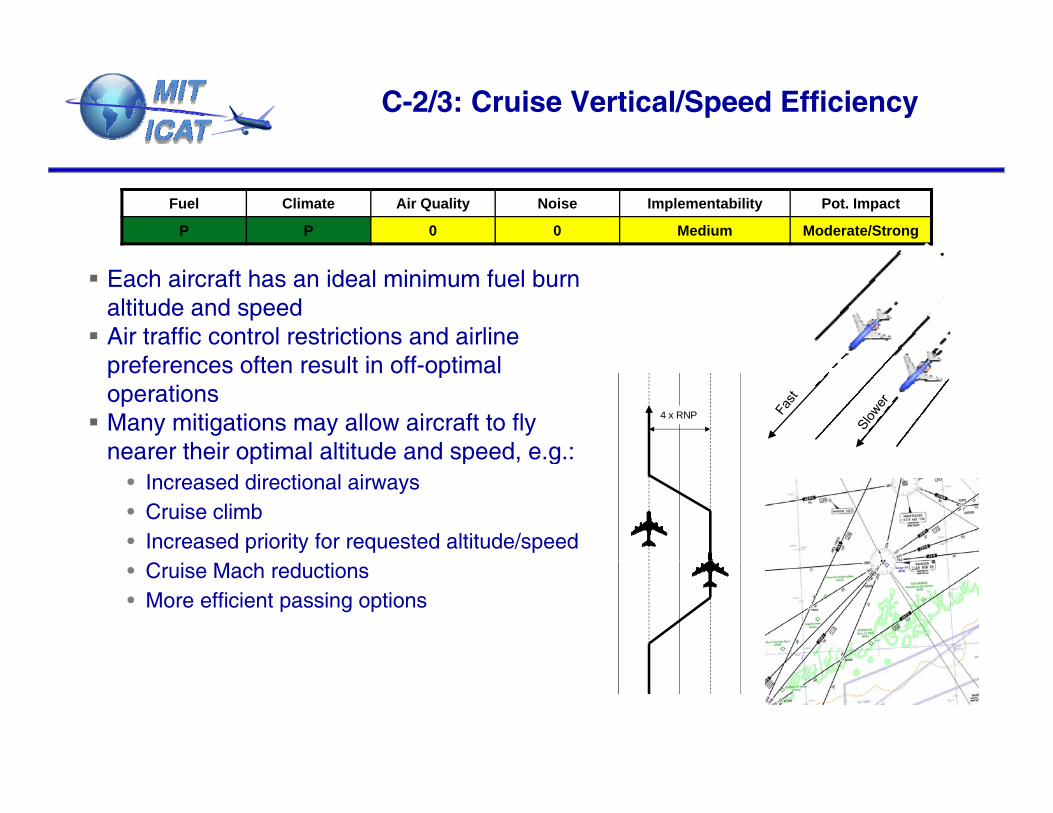
Piano-X Aircraft Performance
Primary focus on Standard Air Range (SAR): distance flown per kg of fuel SAR table of speed vs altitude mapped for
Utilized step climb profiles in Piano-X to match optimum altitude with weight
• Validated results by checking that weight p ppeach aircraft at one weight Fundamental correlation applied to include
SAR sensitivity to weight
changed approximately proportionally with air density
-10
-10
-5-5
-5
400
420
B737-700 SAR (% Below Max) B757-200 Altitude Sensitivity
370
380
FL)
5
-10
5
-5
tude
(10
0s f
t)
360
380
350
360
370
Optimal Altitude
(F
-2520-15
-15
-15
-10-10
-10-5-5Alti
t
300
320
340
330
340
85000 90000 95000 100000 105000 110000 115000
O
Aircraft Weight (kg)
6
-20
Mach
0.7 0.72 0.74 0.76 0.78 0.8

Standard Air Range Comparison
-10
-10
-5-5
400
420
B737-700 SAR (% below max)-20-15 -15-10
-10-5
-5 -5400
A320-200 SAR (% below max)-5 -5440
CRJ-200 SAR (% below max)
-15
0
-10-1
0
-5
-5
-5-5
Alti
tude
(10
0s f
t)
340
360
380
400
5
0
-10
-5
-5-5
-5
Alti
tude
(10
0s f
t)
340
360
380
105 -5-5
-5
Alti
tude
(10
0s f
t)
360
380
400
420
-25-20-15
-15-10-10
Mach
A
0.7 0.72 0.74 0.76 0.78 0.8
300
320
-20
-15
-15
-10-10-10
Mach
A
0.7 0.72 0.74 0.76 0.78 0.8
300
320
-15
-15-10-10
-10-5
Mach
A
0.7 0.72 0.74 0.76 0.78 0.8
320
340
-20 -20-15 -15
-15-10
-10 -10
-10
-5-5
-5
s ft
)
380
400
B757-200 SAR (% below max)-20
-20-15 -15
-15
-10
-10-10
-10-5 -5
-5
s ft
)
360
380
400
MD82 SAR (% below max)
SAR contours represent performance sensitivity to speed and altitude, at a single
-10
0
-5
-5-5
-5
Alti
tude
(10
0s
320
340
360
1510
-10
0
-5
-5-5
Alti
tude
(10
0s
300
320
340
360 speed and altitude, at a single weight
SAR increases approximately linearly as weight decreases
7
-10
Mach0.72 0.74 0.76 0.78 0.8 0.82
300 -15
-10-10
Mach0.7 0.72 0.74 0.76 0.78 0.8
280
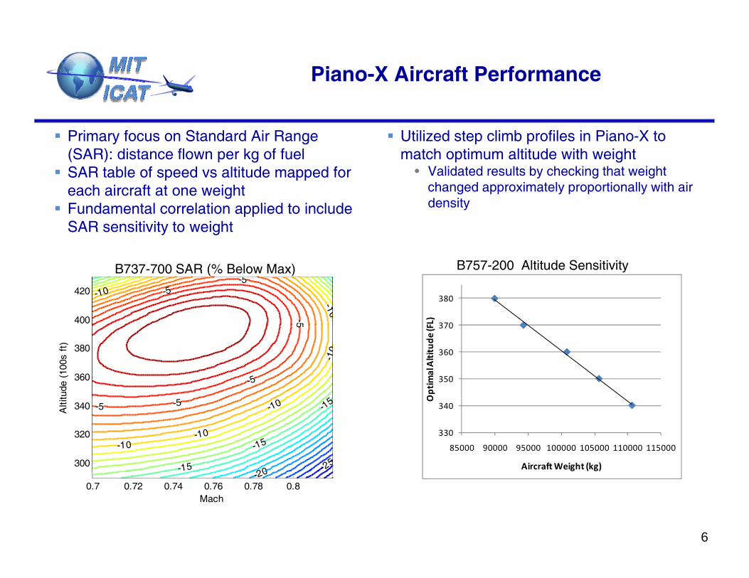
Flight Path Detailed Breakdown
0 100 200 300 400 500 600 700
Distance(nm)
400
Single Segment
200
300
400
de (
100s
ft)
γ
Al i d
Cruise ClimbAngle
0 20 40 60 80 100 1200
100Alti
tu
Minutes
DistanceAltitude
0 100 200 300 400 500 600 700
Distance (nm)
0.8
1 Actual speed calculationnoisy due to limited ETMS position
0.2
0.4
0.6
Mac
h
Speed
accuracy
Moving average smoothes data for
8
0 20 40 60 80 100 1200
Minutes
smoothes data for processing
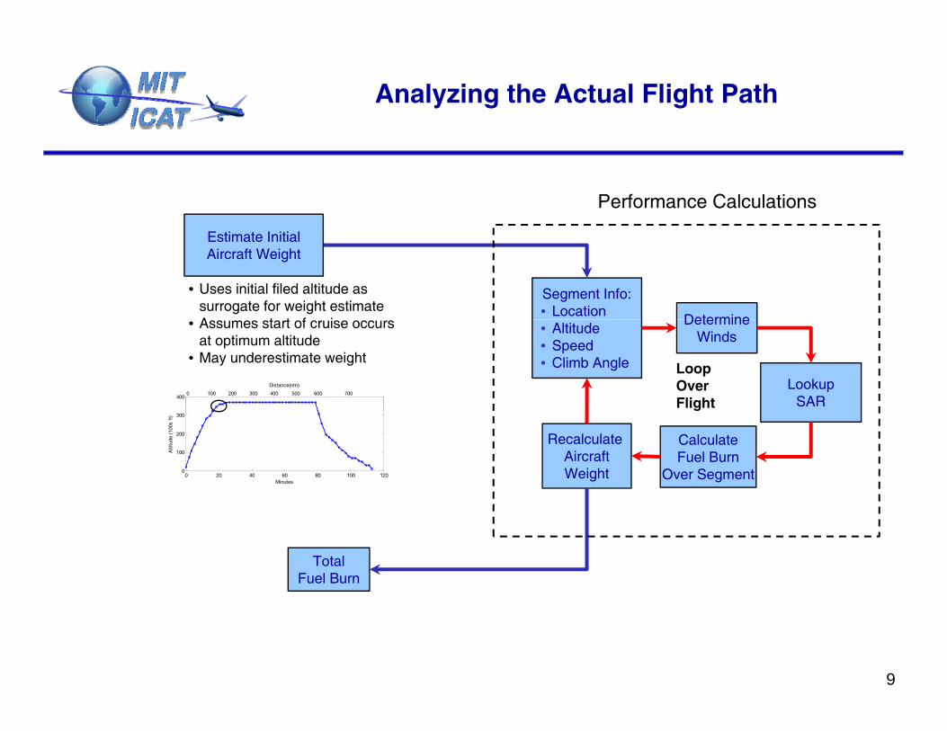
Analyzing the Actual Flight Path
Performance Calculations
Determine
Estimate InitialAircraft Weight
Segment Info:• Location
• Uses initial filed altitude as surrogate for weight estimateA t t f i Determine
Winds
LookupSAR
• Altitude• Speed• Climb Angle
• Assumes start of cruise occurs at optimum altitude
• May underestimate weight
0 100 200 300 400 500 600 700
Distance(nm)
400
LoopOver Flight
CalculateFuel Burn
Over Segment
RecalculateAircraftWeight0 20 40 60 80 100 120
0
100
200
300
Alti
tude
(10
0s f
t)
Minutes
TotalFuel Burn
9

Developing The Ideal Flight Path
Estimate InitialAircraft Weight
Performance CalculationsCruise ClimbAngle
Determination
DetermineWinds
Segment Info:• Location• Altitude• Speed• Climb Angle
Determination
•Uses same weight determined in “actual” fuel burn calculation
Select SpeedThat MinimizesWind-Adjusted
SAR
Climb Angle
LoopOver Flight
DetermineIdeal Alt
CalculateFuel Burn
Over Segment
RecalculateAircraftWeight
Minimum Cruise Climb 390
400
410
e (F
L)
Actual
Ideal
10
Fuel Burn Path
Best Case 0 500 1000 1500 2000360
370
380
Alti
tud

Sample Flight: B757-200 from BOS to SFO
0.9Speed Profile
Fuel Burn Savings
2 88% Total
Altitude Profile
390
400 Actual
Ideal (pres)Ideal (dens)
0.7
0.8
Mac
h
2.88% Total 0.57% from
altitude-only improvement
2.16% from speed-only
Headwind increases ideal airspeed
360
370
380
Alti
tude
(F
L)
Ideal (dens)
0 500 1000 1500 2000 25000.5
0.6
Dist (nm)
yimprovement
0 500 1000 1500 2000 2500340
350
360
Dist (nm)
A
20
40
s) 0.16
0.18
Persisting
Tailwind Profile Instantaneous Standard Air Range (SAR, nm/kg)
( )
40
-20
0
Gsp
d-A
spd
(kts
0.12
0.14
SA
R (
nm/k
g) operations below the “ideal” SAR line indicate improvement potential
Headwind
0 500 1000 1500 2000 2500-60
-40
Dist (nm)0 500 1000 1500 2000 2500
0.1
Dist (nm)
Spikes correlate with climbs and descents
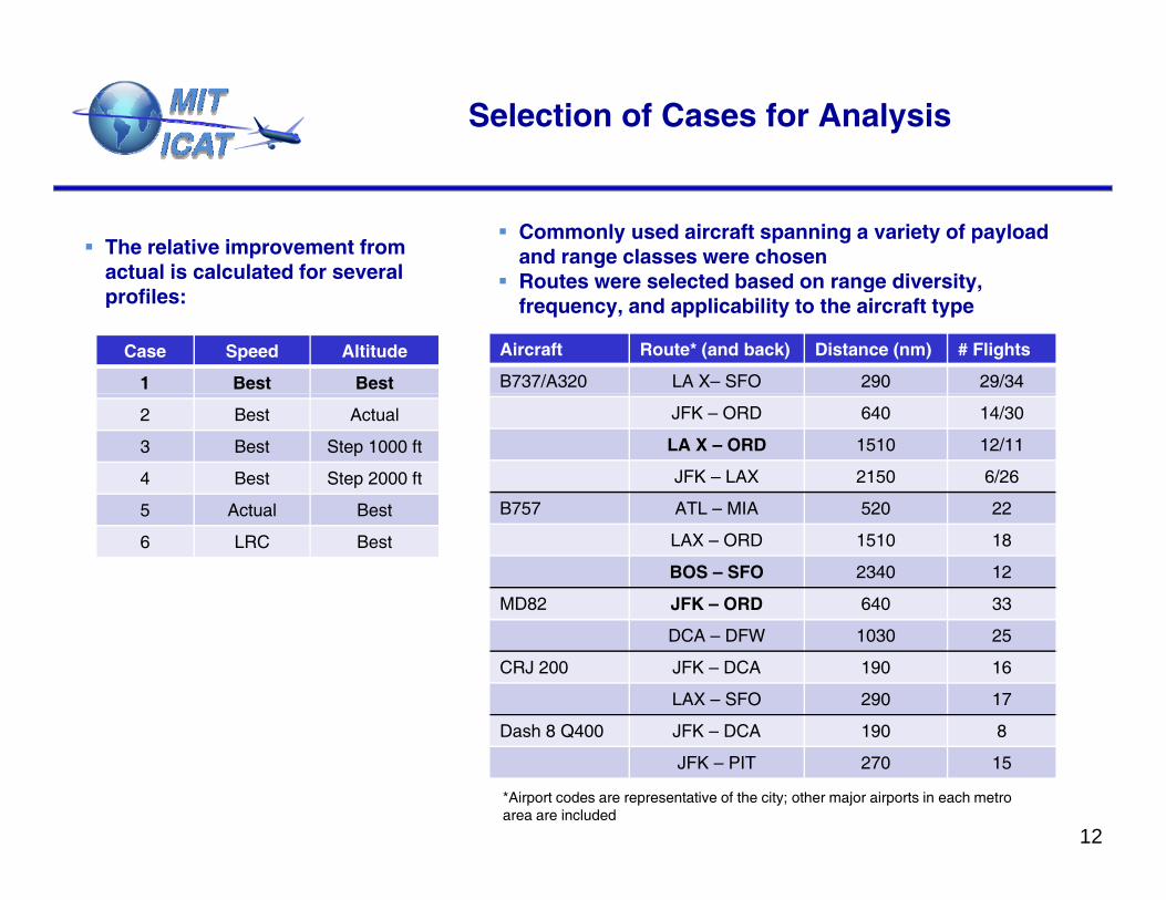
Selection of Cases for Analysis
The relative improvement from actual is calculated for several
Commonly used aircraft spanning a variety of payload and range classes were chosen
Routes were selected based on range diversity profiles:
Case Speed Altitude
1 Best Best
Aircraft Route* (and back) Distance (nm) # Flights
B737/A320 LA X– SFO 290 29/34
Routes were selected based on range diversity, frequency, and applicability to the aircraft type
2 Best Actual
3 Best Step 1000 ft
4 Best Step 2000 ft
5 Actual Best
JFK – ORD 640 14/30
LA X – ORD 1510 12/11
JFK – LAX 2150 6/26
B757 ATL MIA 520 225 Actual Best
6 LRC Best
B757 ATL – MIA 520 22
LAX – ORD 1510 18
BOS – SFO 2340 12
MD82 JFK – ORD 640 33
DCA – DFW 1030 25
CRJ 200 JFK – DCA 190 16
LAX – SFO 290 17
Dash 8 Q400 JFK – DCA 190 8
12
Dash 8 Q400 JFK DCA 190 8
JFK – PIT 270 15
*Airport codes are representative of the city; other major airports in each metro area are included

Secondary Effects
Temperate deviations from ISA can be significant
• ISA + 10C at FL390 increases density altitude
Extra fuel is burned in the cruise climb This is mostly recovered in descent, but ISA + 10C at FL390 increases density altitude
by 1000 ft• Cruise climbs are on the order of 1000s feet
Optimal altitude is a function of density altitude, but aircraft fly pressure altitude
must be included A cruise climb, excluding the benefit of
descent, can appear worse than level flight
Maintaining correct density altitude can mean unusual profiles
B737-700Los Angeles to Chicago
398
400
402
404)
Actual
Ideal (dens)
Ideal (pres)-50
-48
C)
Actual
ISA
Descent must be included to make up for climb energy
392
394
396
398
Alti
tude
(F
L)
56
-54
-52
Tem
pera
ture
(C
Non standard temperatures can lead to unusual altitude profiles
13
0 200 400 600 800 1000 1200 1400388
390
Dist (nm)
0 500 1000 1500
-58
-56
Distance (nm)

Long Range Example: B757-200
Boston – San Francisco (2,340 nm) B757-200 Headwind Case 4
5
6
men
t
Speed
Altitude
Avg Improvement: 3.73%• Altitude Alone: 1.36%• Speed Alone: 2.52%
1
2
3
% I
mpr
ovem
370
380
390
400
e (F
L)
Actual
Ideal(d)
360
370
380
390
e (F
L) 360
370
380
e (F
L) 360
370
380
e (F
L)
1 2 3 40
0 500 1000 1500 2000 2500340
350
360
370
Dist (nm)
Alti
tud
0 500 1000 1500 2000 2500
320
330
340
350
Dist (nm)
Alti
tude
0 500 1000 1500 2000 2500330
340
350
Dist (nm)A
ltitu
de0 500 1000 1500 2000 2500
330
340
350
Dist (nm)
Alti
tud
2
0.7
0.8
0.9
Mac
h
0.7
0.8
0.9
Mac
h
0.7
0.8
0.9
Mac
h
0 7
0.8
0.9
1
Mac
h
1 2 3 4
0 500 1000 1500 2000 25000.5
0.6
Dist (nm)0 500 1000 1500 2000 2500
0.5
0.6
Dist (nm)0 500 1000 1500 2000 2500
0.5
0.6
Dist (nm)0 500 1000 1500 2000 2500
0.5
0.6
0.7
Dist (nm)
14
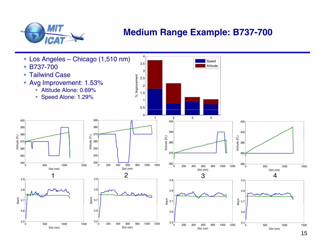
Medium Range Example: B737-700
Los Angeles – Chicago (1,510 nm) B737-700 Tailwind Case
2 5
3
3.5
4
ent
Speed
Altitude
Avg Improvement: 1.53%• Altitude Alone: 0.69%• Speed Alone: 1.29%
0.5
1
1.5
2
2.5
% I
mpr
ovem
e
370
380
390
400
e (F
L)
360
370
380
390
e (F
L)
390
400
e (F
L)
400
405
e (F
L)
1 2 3 40
0 500 1000 1500340
350
360
370
Dist (nm)
Alti
tude
0 200 400 600 800 1000 1200330
340
350
360
Dist (nm)
Alti
tud
0 200 400 600 800 1000 1200360
370
380
Dist (nm)A
ltitu
de0 500 1000 1500
385
390
395
Dist (nm)
Alti
tude
2
0.7
0.8
0.9
Mac
h
0.7
0.8
0.9
Mac
h
0.7
0.8
0.9
Mac
h
0.7
0.8
0.9
Mac
h
1 2 3 4
0 500 1000 15000.5
0.6
Dist (nm)0 200 400 600 800 1000 1200
0.5
0.6
Dist (nm)0 200 400 600 800 1000 1200
0.5
0.6
Dist (nm)0 500 1000 1500
0.5
0.6
Dist (nm)
M15

Short Range Example: MD82
New York – Chicago (640 nm) MD82 Avg Improvement: 1.81% 2.5
3
3.5
nt
Speed
Altitude
g p• Altitude Alone: 0.35%• Speed Alone: 1.68%
0 5
1
1.5
2
% I
mpr
ovem
en
310
315
320
L) 340
350
360
L) 310
315
320
L)
320
330
L)
1 2 3 4 5 6 7 8 9 10 110
0.5
0 50 100 150 200 250 300 350290
295
300
305
Dist (nm)
Alti
tude
(F
L
0 100 200 300 400310
320
330
340
Dist (nm)
Alti
tude
(F
0 100 200 300 400290
295
300
305
Dist (nm)
Alti
tude
(F
L
0 100 200 300 400290
300
310
Dist (nm)
Alti
tude
(F
L
Dist (nm)
0.7
0.75
0.8
Mac
h
( )
0.7
0.8
0.9
Mac
h
Dist (nm)
0.7
0.8
0.9
Mac
h
Dist (nm)
0.7
0.8
0.9
Mac
h
1 2 3 6
0 50 100 150 200 250 300 3500.55
0.6
0.65
Dist (nm)
M
0 100 200 300 4000.5
0.6
Dist (nm)
M
0 100 200 300 4000.5
0.6
Dist (nm)
M
0 100 200 300 4000.5
0.6
Dist (nm)
M16

Short Range Example: B737
2 5%
3.0%
3.5%
4.0%
ent
Altitude
Speed
5 0%
6.0%
7.0%
8.0%
ent
Altitude
Speed B737, New York –
Chicago (640 nm) Eastbound Avg : 1.37%
Eastbound Westbound
0.5%
1.0%
1.5%
2.0%
2.5%
% Im
prov
eme
1.0%
2.0%
3.0%
4.0%
5.0%
% Im
prov
emeg
• Altitude Alone: 1.10%• Speed Alone: 0.83%
Westbound Avg: 3.31%• Altitude Alone: 1.71%• Speed Alone: 2 25%
400
L)
400
L)
380
400
L) 390
400
L)
0.0%1 2 3 4 5 6 7
0.0%1 2 3 4 5 6 7
• Speed Alone: 2.25%
0 200 400 600300
350
Alti
tud
e (
FL
0 100 200 300 400300
350
Di t ( )
Alti
tud
e (
F
0 0 200 400 600340
360
380
Alti
tud
e (
FL
0 100 200 300 400360
370
380
Alti
tud
e (
FL
Earlier step-downsEarlier step-downs
Dist (nm)
0.7
0.8
Ma
ch
Dist (nm)
0.7
0.8
Ma
ch
Dist (nm)
0.7
0.8
Ma
ch
Dist (nm)
0.7
0.8
Mac
h
2 5 2 6
0 200 400 6000.5
0.6
Dist (nm)
M
0 100 200 300 4000.5
0.6
Dist (nm)
M
0 0 200 400 6000.5
0.6
Dist (nm)
M
0 100 200 300 4000.5
0.6
Dist (nm)
M
17

Altitude Sensitivity Example
Washington – Dallas (1,030 nm) MD82 Avg Improvement: 2.30% 3
3.5
4
4.5
ent
Speed
Altitude
g p• Altitude Alone: 1.40%*• Speed Alone: 1.35%
*Results possibly skewed by weight estimate Sensitivity to weight estimate for #3, 5, and 1
1.5
2
2.5
% I
mpr
ovem
e
340
350
)
Actual
Ideal
330
340
350
)
320
330
)
340
350
)
9 examined1 2 3 4 5 6 7 8 9 10 11 12 13
0
0.5
0 200 400 600 800310
320
330
Di t ( )
Alti
tude
(F
L)
0 200 400 600 800
290
300
310
320
330
Dist (nm)
Alti
tude
(F
L)
0 200 400 600 800290
300
310
Dist (nm)
Alti
tude
(F
L)
0 200 400 600 800310
320
330
Di t ( )
Alti
tude
(F
L)
Dist (nm)
0.7
0.8
0.9
ach
Dist (nm)
0.7
0.8
0.9
Mac
h
Dist (nm)
0.7
0.8
0.9
Mac
h
Dist (nm)
0.7
0.8
0.9
ach
3 5 7 9
0 200 400 600 8000.5
0.6
Dist (nm)
M
0 200 400 600 8000.5
0.6
Dist (nm)
M
0 200 400 600 8000.5
0.6
Dist (nm)
M
0 200 400 600 8000.5
0.6
Dist (nm)
M
18

Altitude Sensitivity Example
Washington – Dallas (1,030 nm) MD82 Avg Improvement: 2.30% 3
3.5
4
4.5
nt
Speed
Altitude
g p• Altitude Alone: 1.40%**• Speed Alone: 1.35%
Altitude improvement potential may be exaggerated due to weight estimateS
1
1.5
2
2.5
3
% I
mpr
ovem
e
340
350
)
Actual
Ideal
330
340
350
)
320
330
)
340
350
)
Sensitivity to weight estimate for #3, 5, and 9 examined 1 2 3 4 5 6 7 8 9 10 11 12 13
0
0.5
0 200 400 600 800310
320
330
Di t ( )
Alti
tude
(F
L)
0 200 400 600 800
290
300
310
320
330
Dist (nm)
Alti
tude
(F
L)
0 200 400 600 800290
300
310
Dist (nm)
Alti
tude
(F
L)
0 200 400 600 800310
320
330
Di t ( )
Alti
tude
(F
L)
Dist (nm)
0.7
0.8
0.9
ach
Dist (nm)
0.7
0.8
0.9
Mac
h
Dist (nm)
0.7
0.8
0.9
Mac
h
Dist (nm)
0.7
0.8
0.9
ach
3 5 7 9
Examined sensitivity to weight estimate on following slide
0 200 400 600 8000.5
0.6
Dist (nm)
M
0 200 400 600 8000.5
0.6
Dist (nm)
M
0 200 400 600 8000.5
0.6
Dist (nm)
M
0 200 400 600 8000.5
0.6
Dist (nm)
M
19
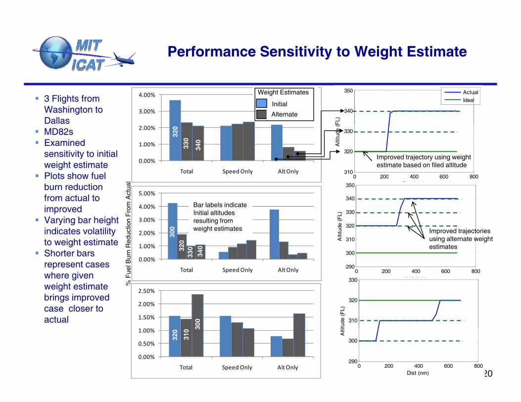
Performance Sensitivity to Weight Estimate
3 Flights from Washington to Dallas
3.00%
4.00%
Initial
Alternate
Weight Estimates
340
350
FL)
Actual
Ideal
MD82s Examined
sensitivity to initial weight estimate
Plots show fuel
0.00%
1.00%
2.00%
Total Speed Only Alt Only0 200 400 600 800
310
320
330
Alti
tude
(
32
0
330
340
Improved trajectory using weight estimate based on filed altitude
Plots show fuel burn reduction from actual to improved
Varying bar height 3.00%
4.00%
5.00%
0 200 400 600 800Dist (nm)
320
330
340
350
de (
FL)
ion
Fro
m A
ctua
l
Bar labels indicate Initial altitudes resulting from
i ht ti tindicates volatility to weight estimate
Shorter bars represent cases where given
0.00%
1.00%
2.00%
Total Speed Only Alt Only 0 200 400 600 800290
300
310
320
Dist (nm)
Alti
tud
Improved trajectories using alternate weight estimates
300
320
330
340
Fue
l Bur
n R
educ
ti weight estimates
where given weight estimate brings improved case closer to actual 1.50%
2.00%
2.50%
Dist (nm)
310
320
330
tude
(F
L)
300
% F
20
0.00%
0.50%
1.00%
Total Speed Only Alt Only 0 200 400 600 800290
300
Dist (nm)
Alti
t
320
310 3

Very Short Range Flights
Short flights often lack significant cruise leg Alternative analysis required to develop
optimum profile
Short flights often cannot reach ideal altitude Operators stay low for speed, simplicity Weight estimation unclearp p
0 50 100 150 200 250 300
Distance(nm)
400 0 50 100 150 200 250 300
Distance(nm)
200
CRJ-200LAX – SFO (290 nm)
Dash 8 Q400JFK – PIT (270 nm)
g
200
300
ltitu
de (
100s
ft)
100
150
titud
e (1
00s
ft)
Ideal trajectories using alternate
0 50 100 150 200 250 300
Distance(nm)
0 10 20 30 40 50 600
100Al
Minutes0 10 20 30 40 50 60 70
0
50Alt
Minutes
Distance(nm)
using alternate weight estimates
0 50 100 150 200 250 300
200
400
de (
100s
ft)
0 50 100 150 200 250 300
100
150
200
de (
100s
ft)
210 10 20 30 40 50 60
0
Alti
tud
Minutes0 10 20 30 40 50 60
0
50Alti
tud
Minutes

Speed and Altitude Optimization Overview
Speed and Altitude Optimization Identified as Potential Opportunity
F d V ti l d S d C i O ti i ti f li it d f fli ht Focused on Vertical and Speed Cruise Optimization for a limited scope of flights and aircraft type
2-5% cruise fuel burn reduction appears possiblepp p• 1-2% from altitude improvements• 2-4% from speed improvements
N t t Next steps• Additional aircraft types and routes• Attempt to obtain data set with actual weights• Larger time scope (more than 1 day)a ge t e scope ( o e t a day)• Include optimal climbs and descents