Quantifying Pavement Albedo Final Report

NCAT Report 19-09

Quantifying Pavement AlbedoFinal ReportDecember 2019

Sponsored byFederal Highway Administration

Office of Infrastructure Research and Development

About the National Concrete Pavement Technology CenterThe mission of the National Concrete Pavement Technology (CP Tech) Center is to unite key transportation stakeholders around the central goal of advancing concrete pavement technology through research, tech transfer, and technology implementation.

About the Institute for Transportation The mission of the Institute for Transportation (InTrans) at Iowa State University is to develop and implement innovative methods, materials, and technologies for improving transportation efficiency, safety, reliability, and sustainability while improving the learning environment of students, faculty, and staff in transportation-related fields.

About the National Center for Asphalt TechnologyThe mission of the National Center for Asphalt Technology (NCAT) at Auburn University is to provide innovative, relevant, and implementable research, technology development, and education that advances safe, durable, and sustainable asphalt pavements.

Iowa State University Nondiscrimination Statement Iowa State University does not discriminate on the basis of race, color, age, ethnicity, religion, national origin, pregnancy, sexual orientation, gender identity, genetic information, sex, marital status, disability, or status as a US veteran. Inquiries regarding nondiscrimination policies may be directed to the Office of Equal Opportunity, 3410 Beardshear Hall, 515 Morrill Road, Ames, Iowa 50011, telephone: 515-294-7612, hotline: 515-294-1222, email: [email protected].

NoticeThis document is disseminated under the sponsorship of the U.S. Department of Transportation (USDOT) in the interest of information exchange. The U.S. Government assumes no liability for the use of the information contained in this document.

The U.S. Government does not endorse products or manufacturers. Trademarks or manufacturers’ names appear in this report only because they are considered essential to the objective of the document. They are included for informational purposes only and are not intended to reflect a preference, approval, or endorsement of any one product or entity.

Non-Binding ContentsThe contents of this document do not have the force and effect of law and are not meant to bind the public in any way. This document is intended only to provide clarity to the public regarding existing requirements under the law or agency policies.

Quality Assurance StatementThe Federal Highway Administration (FHWA) provides high-quality information to serve Government, industry, and the public in a manner that promotes public understanding. Standards and policies are used to ensure and maximize the quality, objectivity, utility, and integrity of its information. FHWA periodically reviews quality issues and adjusts its programs and processes to ensure continuous quality improvement.

Technical Report Documentation Page

1. Report No.

NCAT Report 19-09

2. Government Accession No.

3. Recipient’s Catalog No.

4. Title and Subtitle

Quantifying Pavement Albedo

5. Report Date

December 2019

6. Performing Organization Code:

7. Author(s)

James Alleman and Michael Heitzman

8. Performing Organization Report No.

9. Performing Organization Name and Address

National Concrete Pavement Technology Center

Iowa State University

2711 South Loop Drive, Suite 4700

Ames, IA 50010-8664

10. Work Unit No.

11. Contract or Grant No.

DTFH61-12-C-00016

12. Sponsoring Agency Name and Address 13. Type of Report and Period Covered

Final Report Office of Infrastructure Research and Development

Federal Highway Administration

6300 Georgetown Pike

McLean, VA 22101-2296

14. Sponsoring Agency Code

15. Supplementary Notes

Visit http://www.cptechcenter.org/ for color pdfs of this and other reports from the National Concrete Pavement Technology

Center and http://eng.auburn.edu/research/centers/ncat/ for this and other reports from the National Center for Asphalt

Technology. The FHWA Contracting Officer’s Technical Representative was Eric Weaver.

16. Abstract

Five portland cement concrete (PCC) and five asphalt concrete (AC) pavement locations at each of seven field testing sites in

the central and eastern United States represented a range of aggregate types, pavement surface ages, and climates. Albedo,

thermal properties, and pavement surface characteristics data were collected, and cores were obtained to measure thermal

properties in the laboratory. Test tracks at Auburn University’s National Center for Asphalt Technology (NCAT) and

Minnesota’s MnROAD facility were used to collect 24-hour measurements for thermal model validation.

The albedo data showed that different parameters influence albedo for AC and PCC pavements, albedo approaches a steady

value over time, and the albedo trends for each site differ. The AC albedo model reasonably predicted albedo over time using

pavement age and coarse aggregate color. However, the PCC albedo model did not predict field albedo using pavement age,

coarse aggregate color, and surface texture; additional field study is needed. Climate-related factors, particularly winter

maintenance activities, may also play a role in pavement albedo.

Pavement thermal modeling required an understanding of the surface and thermal properties, small incremental units of time

and layer thicknesses, 10 to 20 days of simulation to achieve balance throughout the pavement and subgrade system, and

continuous data over an extended period. The thermal model predicted pavement thermal response in warm, dry conditions

but did not account for the influence of moisture and freezing conditions.

Asphalt and concrete thermal properties vary and may have up to a 15% influence on AASHTOWare Pavement ME Design

results. Current highway sustainability rating systems have recognized the complexity of pavement albedo, and the current

systems either only address qualitative cool pavement goals or have no coverage of albedo-related metrics or outcomes.

17. Key Words

asphalt concrete—pavement albedo model—pavement heat

capacity—Pavement ME Design—pavement surface emissivity—

pavement thermal conductivity—pavement thermal model—

portland cement concrete—sustainability rating systems

18. Distribution Statement

No restrictions.

19. Security Classif. (of this report)

Unclassified

20. Security Classif. (of this page)

Unclassified

21. No. of Pages

232

22. Price

N/A

http://www.cptechcenter.org/

http://eng.auburn.edu/research/centers/ncat/

QUANTIFYING PAVEMENT ALBEDO

Final Report

December 2019

Principal Investigators

James Alleman, Professor

Civil, Construction, and Environmental Engineering


Michael Heitzman, Assistant Director and Senior Research Engineer

National Center for Asphalt Technology

at Auburn University

Co-Principal Investigator

Peter Taylor, Director



Authors

James Alleman and Michael Heitzman

Sponsored by

Federal Highway Administration

(NCAT Report 19-09)

A report from

National Center for Asphalt Technology

at Auburn University

277 Technology Parkway

Auburn, AL 36830




2711 South Loop Drive, Suite 4700

Ames, IA 50010-8664

Phone: 515-294-8103 / Fax: 515-294-0467

https://cptechcenter.org/


https://cptechcenter.org/

v

TABLE OF CONTENTS

ACKNOWLEDGMENTS .............................................................................................................xv

LIST OF ACRONYMS AND ABBREVIATIONS ................................................................... xvii

EXECUTIVE SUMMARY ......................................................................................................... xxi

CHAPTER 1. INTRODUCTION ....................................................................................................1

Pavement Albedo Fundamentals................................................................................................1 Pavement Albedo Implications ..................................................................................................3

Pavement Solar Energy Capture and Release ......................................................................3 Cool Pavements and Urban Heat Island Effects ..................................................................3 Thermal Effects on Pavement Performance ........................................................................5

Pavement Sustainability and Design ....................................................................................5

CHAPTER 2. PROJECT SCOPE, HYPOTHESES, OBJECTIVES, AND OUTCOMES .............7

Scope ..........................................................................................................................................7 Hypotheses .................................................................................................................................7

Objectives ..................................................................................................................................8 Outcomes ...................................................................................................................................8

CHAPTER 3. LITERATURE ........................................................................................................10

Pavement Albedo Property ......................................................................................................10 Pavement Albedo Analysis Procedures .............................................................................10

Pavement Albedo Testing Citation Overview ...................................................................14 Roofing Albedo Testing Citation Overview ......................................................................16

Pavement Albedo Variability .............................................................................................18 Pavement Thermal Properties ..................................................................................................26

Thermal Conductivity ........................................................................................................26 Specific Heat ......................................................................................................................27

Emissivity ..........................................................................................................................28 Density ...............................................................................................................................28 Heat Flux ............................................................................................................................29

Pavement Thermal Modeling ...................................................................................................29 Sustainability Rating Systems Relative to Albedo Properties and Cool Pavement Issues ......31

CHAPTER 4. PAVEMENT THERMAL MODELING ................................................................34

Pavement Thermal Dynamics ..................................................................................................34

Pavement Albedo Modeling Background ................................................................................36

Environmental Location.....................................................................................................42 Pavement Thermal Model Development .................................................................................42

CHAPTER 5. METHODOLOGY .................................................................................................48

General Work Plan ...................................................................................................................48 Work Plan Variable Overview ...........................................................................................51

Factors Integrated into Albedo Modeling ..........................................................................52 Factors Integrated into Pavement Thermal Modeling .......................................................55

vi

City Testing Locations and Planning .................................................................................57

Test Track Testing Locations and Planning.......................................................................60

Field Analytical Testing and Sampling....................................................................................60 Pavement Albedo Measurement ........................................................................................61 Pavement Coring Procedures .............................................................................................63 Pavement Temperature Measurement ................................................................................63 Pavement Texture Measurement........................................................................................64

Surface Color .....................................................................................................................65 Emissivity ..........................................................................................................................66 Pavement Heat Flux Measurement ....................................................................................66

Laboratory Pavement Core Material Characteristics Testing ..................................................67 Thermal Conductivity ........................................................................................................67

Specific Heat Capacity .......................................................................................................69

Emissivity ..........................................................................................................................70 Density ...............................................................................................................................70

Surface and Aggregate Color .............................................................................................70

Weather Monitoring ...........................................................................................................71 Completeness of the Field and Laboratory Testing Plan .........................................................72

CHAPTER 6. RESULTS AND DISCUSSION .............................................................................87

Pavement Albedo .....................................................................................................................87 City-Specific Pavement Albedo Measurements ................................................................87

Comprehensive City-Level AC Pavement Albedo Results ...............................................95 Comprehensive City-Level PCC Pavement Albedo Results .............................................97 City-Specific 10-hour Tracking Results ............................................................................97

Test Track Pavement Albedo Results ................................................................................98

Pavement Core Properties Findings .........................................................................................98 City Testing Results ...........................................................................................................98

Pavement Albedo Modeling ..................................................................................................107

City Testing Results .........................................................................................................107 Pavement Thermal Modeling .................................................................................................134

MnROAD Test Track Model Results ..............................................................................134

Alternative Pavement Thermal Model Cross-Correlation ...............................................143 Pavement Thermal Model Integration with MEPDG and AASHTOWare Pavement ME

Design ..............................................................................................................................145 Sustainability Assessment ......................................................................................................151

CHAPTER 7. FINDINGS AND PERSPECTIVES .....................................................................153

City-Level Pavement Testing Outcomes ...............................................................................153 General Overview of City-Level Testing ........................................................................153

City-Level Pavement Albedo Results ..............................................................................154 Albedo Aging Factor Assessment ..........................................................................................157 Laboratory Pavement Core Results .......................................................................................159

Thermal Conductivity ......................................................................................................159 Specific Heat ....................................................................................................................160 Emissivity ........................................................................................................................161 Density .............................................................................................................................162

vii

Modeling Outcomes ...............................................................................................................163

Pavement Albedo Model..................................................................................................163

Pavement Thermal Model ................................................................................................164 Pavement Design Model Integration Outcomes (PAVE me) ................................................165 Sustainability Advocacy and Rating System Integration Outcomes .....................................166 Analytical Outcomes ..............................................................................................................167

Lessons Learned About Finding Host Cities and Site Selection .....................................167

Lessons Learned About Field Site Testing ......................................................................168 Lessons Learned About Laboratory Testing ....................................................................169

Recommended Further Research ...........................................................................................170 Validation of Albedo Model for Asphalt Pavements .......................................................170 Broaden the PCC Pavement Surface Albedo Investigation .............................................170

Wet and Frozen Pavement Thermal Modeling Investigation ..........................................170

Pavement Aggregate Material Characteristics Investigation ...........................................170 Advancement of the Testing Protocols for Measuring Pavement Core Thermal

Properties ...................................................................................................................171

REFERENCES ............................................................................................................................173

APPENDIX A: PAVEMENT CORE TESTING LABORATORY METHODS ........................181

Surface Emissivity Test .........................................................................................................181

Calibration Step 1 ............................................................................................................181 Calibration Step 2 ............................................................................................................182

Calibration Step 3 ............................................................................................................182 Testing..............................................................................................................................182

Thermal Conductivity Test ....................................................................................................182

Test Preparation ...............................................................................................................182

Testing..............................................................................................................................187 Calculation .......................................................................................................................188 Test Results ......................................................................................................................189

Test Limitations ...............................................................................................................189 Heat Capacity Test .................................................................................................................190

Test Preparation ...............................................................................................................190

Testing..............................................................................................................................192 Calculation .......................................................................................................................194 Test Results ......................................................................................................................195

Aggregate Grayscale Color Analysis .....................................................................................197 Preparation for the Procedure ..........................................................................................197

Steps to Determine Aggregate Grayscale Value ..............................................................198

APPENDIX B: PAVEMENT THERMAL MODEL USER GUIDE ..........................................201

Step #1 ...................................................................................................................................202 Step #2 ...................................................................................................................................203 Step #3 ...................................................................................................................................204 Step #4 ...................................................................................................................................206 Step #5 ...................................................................................................................................207

viii

LIST OF FIGURES

Figure 1. Pavement albedo assessment - MnROAD test track site..................................................2

Figure 2. Urban heat island profile ..................................................................................................4 Figure 3. Correlation between urban air temperature and ozone presence at Des Moines,

Iowa .................................................................................................................................5 Figure 4. Albedometer approximate cross-section using dual-pyranometer setup ........................12 Figure 5. Albedometer test stand mounting ...................................................................................13

Figure 6. Solar spectrum reflectometer ..........................................................................................14 Figure 7. AC pavement daily albedo variability ............................................................................18 Figure 8. PCC pavement daily albedo variability ..........................................................................19 Figure 9. AC pavement seasonal albedo variation.........................................................................20 Figure 10. Theoretical seasonal albedo sinusoidal pattern ............................................................21

Figure 11. AC pavement albedo aging ..........................................................................................23 Figure 12. Pavement albedo aging .................................................................................................24

Figure 13. Richard pavement albedo aging plot ............................................................................24 Figure 14. Asphalt pavement albedo aging....................................................................................25

Figure 15. Albedo aging data plot and model ................................................................................26 Figure 16. Basic thermal model (day)............................................................................................35 Figure 17. Basic thermal model (night) .........................................................................................36

Figure 18. Basic albedo model.......................................................................................................36 Figure 19. Properties of mature, unexposed concrete. ...................................................................38

Figure 20. Cementitious material color variation ..........................................................................39 Figure 21. Surface temperature and albedo for selected types of pavements in Phoenix,

Arizona ..........................................................................................................................40

Figure 22. Paint-coated asphalt pavement .....................................................................................41

Figure 23. Convective heat transfer ...............................................................................................43 Figure 24. Convective heat transfer coefficient h derivation .........................................................44 Figure 25. Convective heat transfer coefficient simplification ......................................................44

Figure 26. Absorbed solar energy ..................................................................................................45 Figure 27. Radiative energy transfer ..............................................................................................46

Figure 28. Background sky temperature derivation .......................................................................46

Figure 29. City-level field testing plan ..........................................................................................48 Figure 30. Test track testing plan ...................................................................................................49 Figure 31. City and test track testing plan .....................................................................................50 Figure 32. City field site testing overview .....................................................................................61 Figure 33. Albedometer sensor system ..........................................................................................62

Figure 34. Albedometer mounting during city field testing ..........................................................62 Figure 35. Thermocouple placement profile ..................................................................................64

Figure 36. Sand patch testing .........................................................................................................65 Figure 37. Surface color chart ........................................................................................................65 Figure 38. Heat flux sensor placement ..........................................................................................66 Figure 39. Heat flux sensor surface positioning ............................................................................66 Figure 40. Installed heat flux sensor with cap cover .....................................................................67

Figure 41. Thermal conductivity laboratory testing setup .............................................................68 Figure 42. Thermal conductivity laboratory testing setup and data collection ..............................68 Figure 43. Specific heat laboratory testing setup ...........................................................................69

ix

Figure 44. Specific heat laboratory testing setup with data collection ..........................................69

Figure 45. Emissivity laboratory testing setup ..............................................................................70

Figure 46. Aggregate color analysis with color chart ....................................................................71 Figure 47. Weather station placement ...........................................................................................72 Figure 48. CP Tech Cape Girardeau, Missouri pavement albedo..................................................87 Figure 49. NCAT Cape Girardeau, Missouri pavement albedo.....................................................88 Figure 50. Greenville, South Carolina pavement albedo ...............................................................89

Figure 51. Austin, Texas pavement albedo ....................................................................................90 Figure 52. Mississippi statewide pavement albedo........................................................................91 Figure 53. South Bend, Indiana pavement albedo .........................................................................92 Figure 54. Sioux Falls, South Dakota pavement albedo ................................................................93 Figure 55. Waterloo, Iowa pavement albedo .................................................................................94

Figure 56. Comprehensive AC pavement albedo results ...............................................................95

Figure 57. Comprehensive AC pavement albedo results plus data from Pomerantz study ...........96 Figure 58. Comprehensive PCC pavement albedo results .............................................................97

Figure 59. PCC thermal conductivity testing results .....................................................................98

Figure 60. PCC thermal conductivity results compared to published values ................................99 Figure 61. AC thermal conductivity testing results .......................................................................99 Figure 62. AC thermal conductivity results compared to published values ................................100

Figure 63. PCC specific heat testing results ................................................................................101 Figure 64. PCC specific heat results compared to published values ...........................................101

Figure 65. AC specific heat testing results ..................................................................................102 Figure 66. AC specific heat results compared to published values .............................................102 Figure 67. PCC emissivity testing results ....................................................................................103

Figure 68. PCC emissivity results compared to published values ...............................................103

Figure 69. AC emissivity testing results ......................................................................................104 Figure 70. AC emissivity results compared to published values .................................................104 Figure 71. PCC density testing results .........................................................................................105

Figure 72. PCC density results compared to published values ....................................................105 Figure 73. AC density testing results ...........................................................................................106

Figure 74. AC density results compared to published values ......................................................106 Figure 75. Asphalt surface albedo change with time ...................................................................107 Figure 76. Concrete surface albedo change with time .................................................................108

Figure 77. Asphalt surface centerline and wheel path color ........................................................109 Figure 78. Concrete surface centerline and wheel path color ......................................................109 Figure 79. Pavement centerline and wheel path color comparison .............................................110

Figure 80. Pavement centerline and wheel path surface texture comparison ..............................111

Figure 81. Asphalt field surface color and laboratory surface color comparison ........................112

Figure 82. Asphalt field surface color and laboratory aggregate color comparison ....................112 Figure 83. Concrete field surface color and laboratory surface color comparison ......................113 Figure 84. Concrete field surface color and laboratory aggregate color comparison ..................113 Figure 85. Printout. Regression analysis of asphalt albedo variables ..........................................115 Figure 86. Printout. Regression analysis of concrete albedo variables........................................116

Figure 87. General form of asphalt albedo model .......................................................................117 Figure 88. Field-measured asphalt surface albedo change with time ..........................................118

x

Figure 89. Relationship of asphalt albedo model constants and location coarse aggregate

color.............................................................................................................................119

Figure 90. Asphalt albedo model using pavement age and aggregate color ................................119 Figure 91. Measured field albedo trend and asphalt model albedo trend ....................................120 Figure 92. Measured asphalt site albedo and asphalt model albedo comparison ........................121 Figure 93. Difference between measure asphalt site albedo and asphalt model-computed

albedo ..........................................................................................................................121

Figure 94. Asphalt albedo model validation measured field trend and computed model

trend.............................................................................................................................122 Figure 95. Asphalt model validation histogram of difference between field-measured

albedo and model albedo .............................................................................................122 Figure 96. Recalibration of asphalt model constants with location aggregate color ...................123

Figure 97. Asphalt albedo model using pavement age and aggregate color ................................123

Figure 98. Asphalt albedo model versus best fit trend.................................................................124 Figure 99. Measured asphalt site albedo and recalibrated model albedo comparison .................126

Figure 100. Difference between measured asphalt site albedo and recalibrated asphalt

model computed albedo ..............................................................................................126 Figure 101. General form of the concrete albedo model .............................................................127 Figure 102. Field-measured concrete surface albedo change with time ......................................127

Figure 103. Relationship of concrete albedo model constants and location surface texture .......129 Figure 104. Relationship of concrete albedo model constants and location coarse

aggregate color ............................................................................................................132 Figure 105. Relationship of concrete albedo model constants and computed aggregate

color/surface texture parameter ...................................................................................133

Figure 106. Concrete albedo model using pavement age and surface texture .............................133

Figure 107. Concrete albedo model using pavement age and aggregate color ............................133 Figure 108. Concrete albedo model using pavement age, surface texture, and aggregate

color.............................................................................................................................133

Figure 109. MnROAD AC pavement actual versus model temperature correlation (~3 cm

depth)...........................................................................................................................135


depth)...........................................................................................................................135 Figure 111. MnROAD AC pavement actual versus model temperature correlation (~15

cm depth) .....................................................................................................................136 Figure 112. MnROAD AC pavement actual versus model temperature correlation (~67

cm depth) .....................................................................................................................136

Figure 113. MnROAD AC pavement actual versus model temperature correlation (~146

cm depth) .....................................................................................................................136


depth)...........................................................................................................................137 Figure 115. MnROAD AC pavement actual versus model temperature correlation (~8 cm

depth)...........................................................................................................................137 Figure 116. MnROAD AC pavement actual versus model temperature correlation (~15

cm depth) .....................................................................................................................138 Figure 117. MnROAD AC pavement actual versus model temperature correlation (~67

cm depth) .....................................................................................................................138

xi


cm depth) .....................................................................................................................138

Figure 119. MnROAD PCC pavement actual versus model temperature correlation (~3

cm depth) .....................................................................................................................139 Figure 120. MnROAD PCC pavement actual versus model temperature correlation (~8




cm depth) .....................................................................................................................140

Figure 124. MnROAD PCC pavement actual versus model heat flux correlation (~3 cm

depth)...........................................................................................................................141 Figure 125. MnROAD PCC pavement actual versus model temperature correlation (~3

cm depth) .....................................................................................................................141





cm depth) .....................................................................................................................143

Figure 130. Alternative FCVM pavement thermal model analysis of MnROAD PCC

pavement measured versus analysis temperature correlation (~3 cm depth) July

26 through August 9, 2014 ..........................................................................................144 Figure 131. Overlaid comparison of actual MnROAD PCC pavement temperature results

versus FCVM thermal modeling results versus this project’s thermal modeling

results at ~3 cm depth July 26 through August 9, 2014 ..............................................145

Figure 132. Thick asphalt pavement predicted rutting performance sensitivity to a range

of asphalt mixture thermal properties .........................................................................148 Figure 133. Thick asphalt pavement predicted fatigue cracking performance sensitivity to

a range of asphalt mixture thermal properties .............................................................148 Figure 134. Thin asphalt pavement predicted rutting performance sensitivity to a range of

asphalt mixture thermal properties ..............................................................................149

Figure 135. Thin asphalt pavement predicted fatigue cracking performance sensitivity to

a range of asphalt mixture thermal properties .............................................................149

Figure 136. Concrete pavement predicted faulting and cracking performance sensitivity

to a range of concrete mixture thermal properties ......................................................150 Figure 137. Relative effect of the range of thermal properties on predicted pavement

performance as a proportion of performance threshold limits ....................................150 Figure 138. General locations for city-level pavement albedo testing ........................................153

Figure 139. Albedo aging results for AC and PCC pavements ...................................................155 Figure 140. PCC albedo aging behavior relative to northern versus southern location ..............156 Figure 141. AC albedo aging behavior relative to northern versus southern location ................157

xii

Figure 142. Core thermal conductivity results .............................................................................159

Figure 143. Core specific heat results ..........................................................................................160

Figure 144. Core emissivity results .............................................................................................162 Figure 145. Core density results ..................................................................................................163 Figure 146. Surface emissivity test setup ....................................................................................181 Figure 147. Thermal conductivity test specimen before upper insulation ...................................184 Figure 148. Thermal conductivity test data logger ......................................................................185

Figure 149. Thermal conductivity test experimental apparatus ...................................................186 Figure 150. Thermal conductivity test equipment setup ..............................................................186 Figure 151. Thermal conductivity test time trace ........................................................................188 Figure 152. Thermal conductivity test equation ..........................................................................188 Figure 153. Heat conductivity of Texas specimens .....................................................................189

Figure 154. Prepared specimens for heat capacity test ................................................................191

Figure 155. Inner views of heat capacity test water chamber ......................................................192 Figure 156. External insulation in the heat capacity test process ................................................193

Figure 157. Heat capacity test assembly ......................................................................................194

Figure 158. Heat capacity test equation .......................................................................................194 Figure 159. Heat capacity test container heat loss without specimen ..........................................195 Figure 160. Heat capacity test time trace .....................................................................................196

Figure 161. Grayscale analysis image station setup ....................................................................198 Figure 162. Rows 1 through 9 and columns A through K of spreadsheet-based pavement

thermal model Sheet #3 ...............................................................................................202 Figure 163. Rows 1 through 9 and columns L through S of spreadsheet-based pavement

thermal model Sheet #3 ...............................................................................................203

Figure 164. Rows 1 through 9 and columns T through AB of spreadsheet-based pavement

thermal model Sheet #3 ...............................................................................................204 Figure 165. Rows 1 through 9 and columns AC through AS of spreadsheet-based

pavement thermal model Sheet #3 ..............................................................................206

Figure 166. Rows 1 through 9 and columns CP through DB of spreadsheet-based

pavement thermal model Sheet #3 ..............................................................................207

xiii

LIST OF TABLES

Table 1. Chronological pavement albedo testing and assessment publications .............................10

Table 2. Chronological pavement albedo testing and assessment publications .............................15 Table 3. Chronological roofing albedo testing and assessment publications ................................17 Table 4. Optimized model parameters ...........................................................................................22 Table 5. PCC and AC thermal conductivity value citations ..........................................................27 Table 6. Published AC and PCC specific heat value citations ......................................................28

Table 7. Published AC and PCC emissivity value citations ..........................................................28 Table 8. Published AC and PCC pavement density value citations ..............................................29 Table 9. Chronological pavement heat flux testing and assessment publications .........................29 Table 10. Chronology of pavement thermal modeling publications..............................................30 Table 11. Sustainability highway infrastructure rating systems and cool pavement aspects ........32

Table 12. General summary of pavement thermal terms and symbols ..........................................34 Table 13. Factorial array of study variables for albedo modeling .................................................54

Table 14. Factorial array of testing variables for heat model study...............................................56 Table 15. Field testing site and location selection criteria and details ...........................................58

Table 16. Cape Girardeau, Missouri city-level site testing details ................................................73 Table 17. Waterloo, Iowa city-level site testing details .................................................................75 Table 18. South Bend, Indiana city-level site testing details .........................................................77

Table 19. Sioux Falls, South Dakota city-level site testing details ................................................79 Table 20. Mississippi (statewide locations) city-level site testing details .....................................81

Table 21. Greenville, South Carolina city-level site testing details ...............................................83 Table 22. Austin, Texas city-level site testing details ...................................................................85 Table 23. Asphalt albedo trend equation constants and aggregate color by field location ..........118

Table 24. Asphalt variables and computed albedo values for each site .......................................125

Table 25. Concrete albedo trend equation constants, texture, and aggregate color by field

location ........................................................................................................................128 Table 26. Concrete variables and computed albedo values for each site .....................................130

Table 27. Thick AC pavement performance prediction results for varying material

thermal properties........................................................................................................146

Table 28. Thin AC pavement performance prediction results for varying material thermal

properties .....................................................................................................................147 Table 29. Concrete pavement performance prediction results for varying material thermal

properties .....................................................................................................................147 Table 30. General summary of perceived aging effect mechanisms for pavement albedo

aging ............................................................................................................................158

Table 31. Heat conductivity of Texas specimens ........................................................................189 Table 32. Heat capacity test numbers for CP Tech Sample 9 ......................................................196

Table 33. Sample grayscale standard sheet..................................................................................197 Table 34. Analytical elements in rows 1 through 9 and columns A through K of

spreadsheet-based pavement thermal model Sheet #3 ................................................202 Table 35. Analytical elements in rows 1 through 9 and columns L through S of

spreadsheet-based pavement thermal model Sheet #3 ................................................204

Table 36. Analytical elements in rows 1 through 9 and columns T through AB of


xiv

Table 37. Analytical elements in rows 1 through 9 and columns AC through AS of


Table 38. Analytical elements in rows 1 through 9 and columns CP through DB of


xv

ACKNOWLEDGMENTS

Extending beyond the financial support and direction provided for this project by the Federal

Highway Administration (FHWA), contributions provided by the following individuals and

organizations during the planning, testing, review, writeup, and final report dissemination phases

of this project are gratefully acknowledged. Individuals are listed under their respective

organizations through which they participated during the study.

FHWA

Eric Weaver, Gina Ahlstrom, Chris Wagner, Max Grogg, Senthil Thyagarajan, Katherine Petros,

Lee Gallivan

National Concrete Pavement Technology (CP Tech) Center

Peter Taylor, Tom Cackler, Sharon Prochnow, Bob Steffes, Xuhao Wang, Fatih Bektas

National Center for Asphalt Technology (NCAT)

Brian Waller, Vicki Adams, Carolina Rodezno, Saeed Maghsoodloo, Richard Willis, Geng Wei

Auburn University

Tom Burch

Institute for Transportation (InTrans) Publications

Pete Hunsinger, Sue Stokke

American Concrete Pavement Association

Leith Wathne

National Asphalt Pavement Association

Howard Marks, Heather Dylla

Lawrence Berkeley National Laboratory – Heat Island Group

Ronnen Levinson

Colorado DOT

Jay Goldbaum

New York State DOT

Paul Krekeler

Mississippi DOT

Bill Barstis, Alex Collum

South Carolina DOT

Brandon Wilson

City of Chicago, Illinois

Janet Attarian

xvi

City of South Bend, Indiana

Erik Horvath, Patrick “Corbitt” Kerr, Patrick Henthorn

City of Sioux Fall, South Dakota

Chad Heathy, Jeff DesLauriers, Wes Phillips

City of Waterloo, Iowa

Eric Thorson

City of Cape Girardeau, Missouri

Tim Gramling, Robert Kutak, Scott Griffith

City of Austin, Texas

Ed Poppitt, Ron Koehn

City of Greenville, South Carolina

Dwayne Cooper

Greenville County, South Carolina

Hesha Gamble

MnROAD Test Track

Ben Worek, Len Palek, Robert Strommen, Jack Herndon, Chavonne Hopson

NCAT Test Track

R. Buzz Powell

xvii

LIST OF ACRONYMS AND ABBREVIATIONS

α˜ albedo

ε emission coefficient (emissivity) of pavement

εa absorption coefficient of pavement

σ Stefan-Boltzmann constant

ΔTs temperature difference of the sample

ΔTw temperature difference of the water

AASHTO American Association of State Highway and Transportation Officials

AC asphalt concrete (pavement)

ACPA American Concrete Paving Association

Aggr or AGGR aggregate

a.m. before noon

ASCE American Society of Civil Engineers

ASTM American Society of Testing and Materials

ASU Arizona State University

BTU British thermal unit

BTU/(hr•ft•°F) thermal conductivity, BTU per hour·foot·degree Fahrenheit

BTU/(lb•°F) thermal heat capacity, BTU per pound·degree Fahrenheit

°C degree Celsius

cd calendar day

CLR color

cm centimeter

comp. composite

cp specific heat

Cp,s specific heat capacity of the sample

CP Tech National Concrete Pavement Technology Center

Cp,w specific heat capacity of the water

CTL centerline

CTM circular texture meter

DOT department of transportation

E emissivity

EB eastbound

EICM Enhanced Integrated Climate Model

°F degree Fahrenheit

FCVM Finite Control Volume Method

FHWA Federal Highway Administration

ft/mi foot per mile

g/cm3 gram per cubic centimeter

h convective heat transfer coefficient

HC heat capacity

HMA hot-mix asphalt

I insolation

in. inch

in/mi inch per mile

InTrans Institute for Transportation

IRI International Roughness Index

xviii

J/(kg•K) joule per kilogram·kelvin

K temperature, in kelvins on the Kelvin scale

k thermal (or heat) conductivity

kJ/(kg•°C) kilojoule per kilogram·degree Celsius

kJ/(kg•K) kilojoule per kilogram·kelvin

kph kilometer per hour

L length or height

LBNL Lawrence Berkeley National Laboratory

LTPP Long-Term Pavement Performance program

MnROAD Minnesota Road Research Project

m meters

ml milliliter

Mod. Moderate

mph mile(s) per hour

Ms mass of the sample

m/sec meter per second

MTD mean texture depth

Mw mass of the water

mv millivolt

NCAT National Center for Asphalt Technology

NCHRP National Cooperative Highway Research Program

NIR near infrared

nm nanometer

Nt not tested

OGFC open graded friction course

Pave ME AASHTOWare Pavement ME Design software

PCC portland cement concrete (pavement)

p.m. afternoon

ppb parts per billion

q"abs solar-absorbed energy transfer

q"cond conduction energy transfer

q"convect convective energy transfer

q"rad radiative energy transfer

q"solar solar energy transfer

r radius

R albedo

R2 coefficient of determination

SA solar absorption

SMA stone mastic asphalt

SMP Seasonal Monitoring Program, part of the LTPP program

SR solar reflectance

SRI solar reflectance index

SSR solar spectrum reflectometer

Std Dev standard deviation

SURF CLR pavement centerline core laboratory measured color

T temperature

xix

Tair temperature, air

Tdp temperature, dew point

TC thermal conductivity or thermocouple

tins insulation thickness

Tm temperature, average

Ts temperature, specimen sensor average or temperature, surface

Tsky temperature, sky

Tw temperature, water sensor average

U wind speed

UHI urban heat island

U.S. EPA United States Environmental Protection Agency

UV ultraviolet

V voltage

vpd vehicles per day

W/m2 watt per square meter

W/(m•°C) watt per meter·degree Celsius

W/(m2•°C) watt per square meter·degree Celsius

W/(m•K) watt per meter·kelvin

W/(m2•K) watt per square meter·kelvin

WP wheel path

yrs years

xxi

EXECUTIVE SUMMARY

PROJECT OBJECTIVE AND SCOPE

This project evaluated, characterized, and quantified albedo and thermal properties of real-world

paving materials. Field-measured pavement albedo and thermal properties were used to develop

predictive albedo and thermal models. These resulting models were then compared to

AASHTOWare Pavement ME Design software and Greenroads or GreenPAVE sustainability

rating systems.

METHODOLOGY AND DATA COLLECTION

Key pavement characteristics to measure in the field were identified, with the extent of field data

collection dependent on project budget and time. A broad range of seven city-level field testing

sites in the central and eastern United States were selected to represent a range of local aggregate

types, pavement types and ages, and climates. Sites included Cape Girardeau, Missouri (central

region); Waterloo, Iowa (northern region); South Bend, Indiana (northeast region); Sioux Falls,

South Dakota (northwest region); state roads in Mississippi (southern region); Greenville, South

Carolina (southeast region); and Austin, Texas (southwest region). Working with host cities and

State agencies was vital to the study, and identifying sites with different aggregate colors was a

primary goal. Ten locations were investigated at each site, including five portland cement

concrete (PCC) and five asphalt concrete (AC) pavements. Pavement ages ranged from less

than 1 to more than 30 years.

Field data collection was limited to a five-day window at each site. Albedo, thermal properties,

and pavement surface characteristics data were collected, and cores were obtained to measure

thermal properties in the laboratory. Combined, a total of 35 asphalt pavements and 35 concrete

pavements were originally planned for evaluation. However, 10% of the locations were removed

from the evaluation due to incorrect surfaces, insufficient data, or site safety concerns.

Test tracks at Auburn University’s National Center for Asphalt Technology (NCAT) and

Minnesota’s MnROAD facility were used to collect 24-hour measurements for thermal model

validation.

DIFFICULTIES WITH FIELD DATA COLLECTION AND LABORATORY

MEASUREMENTS

The following difficulties were encountered during field data collection:

• Traffic lanes with the required diverse pavement types and ages that were also safe for lane

closures needed to be identified.

• Data collection needed to be coordinated within a one-week window and with proper weather

conditions.

• Data collection at the two PCC and two AC sites at the MnROAD facility was limited to only

non-winter months due to snow cover.

• Data collection at the NCAT test track was limited to asphalt sections because there was no

practical means of obtaining 24-hour PCC data at this track.

xxii

• Cores obtained from field sites needed to be evaluated in the laboratory for density,

emissivity, thermal conductivity, and specific heat capacity.

The following difficulties were encountered during laboratory measurements:

• No standard test method exists for using core specimens. Both laboratories used in this study

were revising their testing protocol while the testing for this project was ongoing.

• The proposed Arizona State University (ASU) testing methods required some changes for

them to be useful in this study.

• Preparing the cores by drilling holes down the center of the cores damaged some cores, was

difficult to control, and was difficult for cores with very hard aggregate.

FINDINGS AND ANALYSIS

Analysis of the pavement albedo data show the following:

• The parameters that influence albedo are different for AC and PCC.

• Albedo approaches a steady value over time.

• The albedo trend was different for each site investigated.

Pavement thermal modeling requirements are as follows:

• An understanding of the pavement’s surface and thermal properties is required.

• Small incremental units of time and layer thicknesses are needed for the model to run

properly.

• Ten to twenty days of continuous simulation are required to achieve thermal balance

throughout the pavement and subgrade system. While the incremental day-to-day changes in

temperature at a 1.2-meter pavement depth are small, temperatures change throughout the

year and influence the pavement’s thermal dynamics at different depths.

• The thermal model requires continuous data over an extended period. Single 24-hour sets of

field data, as planned for this study, are insufficient to validate the model. Only the

MnROAD locations had a system in place to collect longer term data.

CONCLUSIONS

The following conclusions can be drawn from this study:

• The albedo model for AC pavements provided reasonable predictions of albedo over time

using pavement surface age and the grayscale color of the asphalt mixture’s coarse aggregate.

• The albedo model for PCC pavements is not ready for use. A model using pavement age, the

grayscale color of the mixture’s coarse aggregate, and surface texture was not able to predict

field albedo measurements. Additional field study is required to determine other pavement

characteristics that influence albedo.

• Climate-related factors, particularly winter maintenance activities, may play a role in

pavement albedo.

xxiii

• The thermal model successfully predicted pavement thermal response in warm, dry

conditions, but the developed model is not capable of incorporating the influence of moisture

and freezing conditions on pavement thermal properties.

• The thermal properties of AC and PCC pavements vary and may have up to a 15% influence

on the performance predicted by AASHTOWare Pavement ME Design software.

• Most highway sustainability rating systems have recognized the complexity of pavement

albedo, and this parameter has consequently been removed from most systems.

FURTHER RESEARCH

Further effort is needed to validate the AC albedo model, and further field measurements are

needed to refine the PCC albedo model. The test methods for measuring the thermal properties of

AC and PCC pavement also need to be improved.

1

CHAPTER 1. INTRODUCTION

PAVEMENT ALBEDO FUNDAMENTALS

The albedo of a pavement surface describes its ability to reflect incoming sunlight and is

quantified on a scale of 0 to 1. The term itself was linguistically derived from the Latin word for

“whiteness” (Coakley 2003). High-albedo pavements, including those constructed or coated with

materials that are whiter or more reflective than ordinary pavements, will reflect more incoming

solar radiation than darker pavements. Solar insolation energy that is not reflected, though, is

absorbed, such that low-albedo pavements will then absorb more of the incoming solar energy

than high-albedo pavements.

The condition of a pavement’s reflectance, however, is more complex than that of its light versus

dark color, particularly given that less than half of sunlight is visible. While color is an excellent

gauge of visible reflectance and often correlates with solar reflectance (albedo), two surfaces of

the same color can have very different albedos. For example, the albedo of a “cool” black surface

can be about 0.40 higher than that of a conventional black surface; see Levinson et al. (2007).

Many pavements also tend to have non-homogenous surface colors associated with the diverse

nature of their basic mix makeup and properties and are subjected to a wide range of

environmental coloration impacts (e.g., surface contaminant buildup with vehicle-released oil,

grease, antifreeze, tire crumb rubber, etc.). In addition, pavements may also have varying degrees

of aggregate material exposure, and the albedo of the aggregate materials differs (perhaps

significantly) from that of the binder (i.e., bitumen and cement).

Another factor is that a pavement’s binder, aggregate, etc. surfaces may vary in terms of the

directionality of their reflectance. While most such surfaces would be expected to have a “matte”

(diffuse) appearance, some materials may have a “specular” (mirror-like) or “glossy” (a first-

surface specular reflectance and a second-surface matte reflectance) character. A matte surface

never forms an image, a specular surface always forms an image, and a glossy surface forms an

image when viewed at an angle far from the surface normal. Real-life examples would include

the “matte” nature of an ordinary sheet of white paper, the “specular” nature of a mirror, and the

“glossy” character of a very smooth surface, such as a dark piece of plastic, where the image

formed by the latter is visible when its surface is viewed tangentially.

The degree of roughness inherent to most pavement surfaces would be seen as a matte surface,

but it could well be that certain coarse and fine pavement aggregate materials would exhibit

varying degrees of glossy reflectance.

This project report documents the findings obtained for real-world pavement albedo values that

were collected during a 2013 to 2016 investigation supported by the Federal Highway

Administration (FHWA). During this evaluation, pavement albedos were measured at seven test

cities and two test tracks, including the MnROAD test track, as shown in Figure 1.

2

Figure 1. Pavement albedo assessment - MnROAD test track site

The intended focus of this work was to quantify the impact of pavement aging on albedo

behavior. Limited prior investigation had been completed on this phenomenon and had largely

focused on asphalt-based pavement surfaces within a single western US location (i.e., San Jose,

California), where the results suggested that an upward shift in albedo would result from

continued asphalt pavement aging (Pomerantz et al. 2005). Prior to this study, however, there

were no published results examining the impact of aging on concrete pavement albedo levels.

This project’s focus on pavement albedo within the transportation sector also complements

another study of albedo properties and behavior in relation to roofing materials, which was

initiated and continues to function under the auspices of the Cool Roof Rating Council (CRRC).

This non-profit educational organization was established to implement and communicate an

accurate radiative energy performance rating system for roof surfaces, support research, and

serve as an educational resource for information on roofing. (see Akbari and Levinson 2008,

Levinson 2012, U.S. EPA 2008a, Menon et al. 2011).

In addition to quantifying changes in pavement albedo in relation to aging, this project report

also covers several additional outcomes generated during this study, including the following:

• The derivation of a mathematical model for predicting age-related pavement albedo values

for either standard portland cement concrete (PCC) or asphalt concrete (AC) surfaces.

• The derivation of a mathematical model for predicting pavement thermal dynamics involving

heat transfer at the pavement, base, and subbase levels.

• An evaluation of sustainable highway infrastructure rating systems in relation to their

consideration (or not) of albedo properties (i.e., corresponding with cool pavement, urban

heat island [UHI], and other impacts).

• An evaluation of pavement design practices connected with the use of mechanistic-empirical

design guidance, relative to the consideration of albedo, to include an assessment of the

impacts that would be experienced if this design practice were to pragmatically account for

pavement albedo variation with aging.

3

PAVEMENT ALBEDO IMPLICATIONS

Pavement Solar Energy Capture and Release

From the point of view of a pavement, the fate of incoming sunlight as being either reflected or

absorbed is very simple. The circumstances and scenarios regarding what happens to these

reflected and absorbed insolation fractions, though, can be highly complex. The following short

synopsis is, therefore, intended to only provide a brief overview of the albedo-related

implications for this science.

Sunlight absorbed by pavements can follow a complex set of thermodynamic pathways,

including conduction, convection, and radiative release as well as intermediate storage prior to

eventual rerelease. This project investigated and modeled these pathways; our pavement heat

transfer model and its results are presented and discussed in Chapters 3, 4, 6, and 7 of this report.

This model provides a means of studying and predicting the impact of varying pavement albedo

levels on the uptake and release of incoming sunlight.

Compared to the solar energy captured by pavements, reflected incoming solar energy is

immediately redirected back into the atmosphere. This reflected energy, however, may then

proceed through various pathways with varying degrees of atmospheric thermal impacts, as

follows: (1) direct radiative passage and departure back through the atmosphere (i.e., with no

further absorption) and (2) secondary sorption of this reflected energy on its reverse passage

back through the atmosphere, perhaps due to capture by airborne contaminants such as carbon

black. At the infrared (IR) end of the solar spectrum, pavement-reflected solar energy might even

lead to the secondary recapture of this reflective light energy as it irradiates and then possibly is

absorbed into surrounding building surfaces. This latter pathway may also work in reverse, in

that incoming solar radiation might be reflected from the same sorts of building surfaces,

windows, etc., thereby possibly leading to additively higher incoming solar energy impacting

pavement surfaces.

These pathways by which original incoming solar insolation energy is transported back through

the Earth’s atmosphere involve a highly complex range of possible collection, capture, reflection,

secondary sorption, and other steps. Collectively, though, these energy pathways establish an

overall atmospheric thermodynamic energy balance that operates on a grand ecosystem level.

The impacts of additional solar energy capture and rerelease by pavements, in relation to a so-

called “radiative forcing” effect, have generated considerable debate. It must be noted, though,

that our project was not designed to explore these radiative forcing mechanisms. Simply put,

there is a massively complex set of possible interactions between solar energy radiation and the

built environment’s pavement, building, roof, and other surfaces, where the modeling and

projections involved operate at an exceedingly high level of mathematical sophistication that far

exceeds this project’s experimental goals.

Cool Pavements and Urban Heat Island Effects

Pavements with lower albedo levels will typically sorb more solar energy and have higher

daytime temperatures, while those with higher albedos will sorb less solar energy and have

cooler daytime temperatures. This correlation is not absolute; some pavements (e.g., pervious

4

concrete) have been known to have lower albedo values and yet remain cooler than regular

concrete surfaces (possibly due to their higher evaporative cooling behavior). However,

excluding these nonstandard pavement options, pavements with higher albedos are typically

considered to be advantageous (especially during summer periods) given their cool pavement

character.

This benefit of cooler surfaces can be particularly important within urban areas, given the

surficial extent of their pavement and roofing coverage, where there is a resultant tendency

toward higher urban versus rural summertime air temperatures. This phenomenon is known as

urban heat island behavior, which was first observed in London (UK) in the early 1800s by Luke

Howard, who stated, “[W]e find London always warmer than the country, the average excess of

its temperature being 1.579° [degrees F][0.877° C]” (cited in Mills 2008). Figure 2 depicts this

effect as a multi-degree temperature increase within urban areas compared to cooler suburban

and rural locations.

Source: U.S. EPA 2003.

Figure 2. Urban heat island profile

This UHI behavior can have several negative effects. For example, urban buildings might

experience a proportionately higher summertime energy cooling demand than comparable

suburban-rural buildings, which in turn further increases CO2 emissions due to the buildings’

increased energy demand. These higher temperatures also further accelerate tropospheric ozone

formation, which in turn further increases subsequent smog production (Kenward et al. 2014).

Figure 3 depicts this correlation between ambient air temperature and ozone presence for the Des

Moines, Iowa area.

5

Used with permission. Copyright © 2014 Climate Central. Kenward et al. 2014.

Figure 3. Correlation between urban air temperature and ozone presence at Des Moines,

Iowa

The combined effect of these higher temperature, ozone, and smog stressors collectively leads to

increased adverse human health effects, particularly among younger and older residents and

those with lung impairments (e.g., asthma), who are more apt to experience respiratory stress

caused by these higher temperatures and air contaminant levels. Lastly, these UHI effects may

also translate into yet another group of adverse economic effects when, for example, shoppers

are unenthused about venturing forth into cities whose air quality is neither pleasant nor healthy.

Thermal Effects on Pavement Performance

Pavement albedo and age-related changes can affect performance in terms of several

temperature-induced changes (e.g., softening, rutting, low-temperature cracking, freeze-thaw

cracking, curling, or warping). With asphalt/AC pavements, these effects are also exacerbated by

the fact that bitumen binder properties and reactions (e.g., thermally catalyzed oxidation) change

in relation to higher or lower operating temperatures. These issues are discussed in Chapter 3 of

this report.

Pavement Sustainability and Design

Albedo also affects a pavement’s sustainability and design properties. For example, one of the

earliest sustainability-related highway infrastructure rating systems (i.e., Greenroads) considers

albedo as a credit point factor. Several other options also refer to the interrelated sustainability

aspects of the cool pavement and urban heat island effects. Some examples are GreenPAVE,

GreenLITES, and the Illinois Livability and Sustainable Transportation [I-LAST] system (see

6

Chapter 5 for further discussion). However, it must be emphasized that the latter concerns

involve factors extending beyond the scope of this project. As for pavement design aspects and

procedures, existing design guide methods also incorporate pavement temperature prediction

capabilities akin to the pavement thermal model being developed for this albedo project.

However, neither of these existing applications (i.e., current sustainability rating systems and

pavement design guide mechanisms) fully capture the dynamic nature of pavement albedo

changes, particularly in regards to pavement aging, weathering, material-related aspects, and

other issues. To date, existing data on pavement albedo behavior, as well as on the broader

context of heat sorption and release within urban areas, have largely been limited to either

laboratory-type testing or highly site-specific field testing. Furthermore, the extent of the prior

data is quite limited. This project accordingly advances the body of knowledge regarding

pavement albedo properties and modeling, such that this information might be considered during

future efforts toward developing sustainability rating systems and implementing pavement

design guides.

7

CHAPTER 2. PROJECT SCOPE, HYPOTHESES, OBJECTIVES, AND OUTCOMES

SCOPE

This FHWA research project was completed to evaluate, characterize, and model albedo and

associated heat sorption and release dynamics as they are experienced with real-world paving

materials. The associated research involved field-level pavement albedo and thermal

measurements, which in turn were used to develop predictive models for albedo and thermal heat

transfer relative to the following variables:

• Pavement type (i.e., asphalt concrete or portland cement concrete).

• Pavement age.

• Pavement mix properties (e.g., granular media color).

• Pavement structural characteristics (e.g., surface roughness).

• Geomorphic solar radiance intensity.

• Local climate exposure.

The scope of this research effort consequently focused on the testing of both PCC-based and AC-

based pavements. The ages of the tested pavements ranged from new construction (i.e., less than

one year) to aged materials extending beyond a timeframe of more than a decade. The project

scope also included pavement albedo modeling and pavement thermal modeling. As qualified

previously, however, this project’s “quantifying pavement albedo” scope was not intended to

cover the broader effort of data collection and modeling that would address all factors connected

with urban heat island effects. Indeed, there are myriad additional material, thermodynamic,

atmospheric, and other factors and interactions affecting solar heat exchange between pavements

and adjacent buildings or between pavements and overlying urban atmospheres. As such, this

project was neither able nor intended to investigate or quantify the related UHI effects on

building heating-ventilation-air-conditioning energy demands, atmospheric soot sources and

effects, human health implications, socioeconomic stress consequences, or similar issues.

HYPOTHESES

1. The level of solar reflectance exhibited by a pavement’s surface, as a function of its albedo

value, will have a significant effect on a pavement’s thermodynamic performance.

2. Pavements with lower albedo values will absorb more insolation, and pavements with higher

albedo values will absorb less.

3. Pavement albedo values are not typically constant; albedo values will change during the

lifetime of a pavement.

4. Asphalt pavement albedos will tend to increase as these pavements age; this increase may be

linked to a progressive decrease in the surficial presence of the asphalt’s darker bitumen

binder and a simultaneous increase in the exposure of lighter and more reflective coarse

aggregate surfaces.

8

5. Concrete pavement albedos will tend to decrease as these pavements age; this decrease may

be linked to the progressive darkening of concrete surfaces caused by various chemical,

physical, and biological effects.

6. In the case of either asphalt or concrete, changes in pavement albedo values over time can be

substantial, which in turn can significantly affect how incoming solar energy is absorbed and

rereleased.

OBJECTIVES

1. Quantify the rate and magnitude of albedo and thermal change (i.e., on a yearly basis) by

pavement type, makeup, time, and location. The study examined albedo and pavement

thermal properties using separate approaches based on the amount of data required for each.

2. Develop two utility models in relation to pavement type and material constituents: (1) a

model to determine the relative effect of albedo on heat collection, storage, and transmission

potential, and (2) a model to determine pavement thermal heat transfer. This project’s albedo

models focused on several key variables (pavement type, pavement age, aggregate color, and

north/south siting geography).

3. Using the utility models developed under the second objective, determine the level of

significance of pavement thermal relationships on various pavement sustainability rating

tools as well as the pavement design procedure outlined in the Mechanistic-Empirical

Pavement Design Guide (MEPDG).

4. Provide recommendations for using the albedo and thermal models to choose appropriate

pavement inputs for pavement sustainability rating tools and pavement design tools.

Here again it must be emphasized that these objectives do not include the collection of data or

the development of analytical models by which the influence of pavements and pavement albedo

levels on urban heat island effects can be fully elucidated.

OUTCOMES

1. Seven US cities were studied during approximately one-week visits in regards to the albedo

properties of their variously aged asphalt and concrete pavement surfaces. Additional

extended (i.e., approximately ten-hour duration) surface, base, and subbase temperature

monitoring was also conducted at each of these cities for one asphalt and one concrete

pavement location.

2. Two additional test track locations (at MnROAD and at NCAT) were similarly studied for a

more extended multi-month period to investigate the same albedo and thermocouple

properties for another set of pavement surfaces, with the intent of using this information to

calibrate our pavement thermal model.

3. A pavement thermal model was developed as an analytical tool to understand the fate and

transfer of solar heat energy on alternative pavement-base-subbase systems and to

predictively assess the effect of albedo variation on this same energy flow.

9

4. A pavement albedo model was developed as a second analytical tool to characterize the

magnitude of solar energy being absorbed and rereleased by pavement surfaces.

5. A relatively large spreadsheet file was assembled with data collected during the course of the

study and is available on the National Concrete Pavement Technology (CP Tech) Center’s

website at https://cptechcenter.org/research/completed/quantifying-pavement-albedo/.

https://cptechcenter.org/research/completed/quantifying-pavement-albedo/

10

CHAPTER 3. LITERATURE

PAVEMENT ALBEDO PROPERTY

Pavement Albedo Analysis Procedures

Albedo Analysis Guidance

Table 1 identifies a set of publications produced by the Lawrence Berkeley National

Laboratory’s (LBNL) Heat Island Group (a group within the LBNL Environmental Energy

Technologies Division) that collectively offer a state-of-the-art summary of the science of

measuring solar reflectance in constructed pavement (as well as roofing) surfaces.

Table 1. Chronological pavement albedo testing and assessment publications

Date Author(s) Title

1996 Akbari et al. 1996 ASTM Standards for Measuring Solar Reflectance and Infrared

Emittance of Construction Materials and Comparing their

Steady-State Surface Temperatures

2008 Akbari et al. 2008 Procedure for Measuring the Solar Reflectance of Flat or

Curved Roofing Assemblies

2009 Levinson 2009 Advances in Measuring Solar Reflectance

2010 Levinson et al. 2010a Measuring solar reflectance – Part I: Defining a metric that

accurately predicts solar heat gain

2010 Levinson et al. 2010b Measuring solar reflectance – Part II: Review of practical

methods

Over the past two decades, a variety of testing methods published by the American Society of

Testing and Materials (ASTM) have been mentioned in the literature on pavement analysis that

addresses the measurement of a pavement’s ability to reflect incoming solar radiation, including

literature on albedo, solar reflectance (SR), and solar reflectance index (SRI). In the context of

heat transfer, albedo is synonymous with solar reflectance. SRI, though, relates the temperature

of a test specimen to those of reference black and white test specimens under certain conditions.

While SRI is computed from solar reflectance and thermal emittance, it is not strictly a solar

reflectance metric.

As documented by Levinson et al. (2010b), there are currently four practical methods for

measuring solar reflectivity:

• Method E1918-06, Standard Test Method for Measuring Solar Reflectance of Horizontal and

Low-Sloped Surfaces in the Field (ASTM 2006)

• Method E1918A, Alternative Pyranometer Technique (non-ASTM) (Akbari et al. 2008)

• Method E903, Standard Test Method for Solar Absorptance, Reflectance, and Transmittance

of Materials Using Integrating Spheres (ASTM 1996)

• Method C1549, Standard Test Method for Determination of Solar Reflectance Near Ambient

Temperature Using a Portable Solar Reflectometer (ASTM 2009)

11

Method E1918-06 is likely the most widely used standard for measuring pavement solar

reflectance as defined by ASTM. This method involves two pyranometer devices to measure

upflux and downflux insolation, respectively, using an array of highly sensitive thermocouples

whose sensory surface constitutes a so-called “thermopile” device (see Kipp & Zonen 2016a for

further technical details regarding pyranometer design, construction, and operation).

Methods E1918-06 and C1549 both measure solar reflectance, but these methods vary

significantly in terms of how they are completed. E1918-06 evaluates the reflectance of natural

solar light at a wavelength range of ~300 nm to ~3,000 nm, while C1549 uses an internal light

source (i.e., a tungsten halogen lamp) and tracks reflected light energy using color filters at four

discrete light wavelengths (i.e., 380 nm for ultraviolet [UV], 500 nm for blue, 650 nm for red,

and 1220 nm for infrared).

ASTM E1918-06 Method

The E1918-06 method is a modified version of an earlier ASTM E1918-97 method, and this

newer method (approved in 2006) is now regarded as the standard protocol for measuring

pavement reflectance (ASTM 2015). This method’s pre-2006 procedure for measuring albedo

relied on the use of a single pyranometer whose orientation would need to be intermittently

flipped upside down so that this one device could then capture both incoming and reflected solar

energy. This method generally provided an accurate means of measuring albedo, but the

intermittent flipping step had both positive and negative aspects. On the negative side,

intermittent flipping required tedious, repetitive care in readjusting the device’s true vertical

orientation and complicated data tracking logistics. These flipping steps could also increase

testing error because the incoming solar radiation and reflected solar radiation were not being

measured at exactly the same time. This effect could be more significant during early morning

and later afternoon time periods when the solar insolation levels were changing more quickly,

such that this method’s albedo testing accuracy could be reduced during these early morning and

late afternoon periods.

The dual-pyranometer approach of method E1918-06 represents a more advanced strategy,

where two identical pyranometers are mounted back-to-back to create a so-called albedometer

device. An upward-facing pyranometer measures incoming solar insolation intensity, and a

downward-facing pyranometer measures the portion of the solar radiation being reflected from

the underlying pavement. Figure 4 depicts a profile view of a commercial albedometer device.

12

Figure 4. Albedometer approximate cross-section using dual-pyranometer setup

The advantage of having two pyranometers is that both can be maintained at a true vertical

orientation (confirmed using the device’s onboard bubble level indicator) without the user having

to reset this orientation after back-and-forth flipping iterations. Because both readings (i.e., for

incoming and reflected solar energy) are recorded at the same time, the ratio of these

simultaneous values is equal to the pavement’s measured albedo value. This method can

continuously monitor the change in albedo value with time. The new E1918-06 method’s dual-

pyranometer has consequently proven to be easier to use and provides for more expedient data

collection, given that it continuously collects both upflux and downflux measurements. However,

any comparison of the one-pyranometer versus the two-pyranometer implementation of method

E1918 should also take into account that the former provides some protection against error in

calibration (signal versus irradiance). For example, if only a single pyranometer is used and that

instrument goes out of calibration, the ratio of upflux to downflux may still be correct. If two

pyranometers are used and only one goes out of calibration, the ratio may be wrong.

Method E1918-06 specifies that the lower pyranometer head should be mounted at 0.5 m (19.7

in.) elevation above the pavement surface. Figure 5 provides a schematic view of this mounting.

Light

Light

UpperDetector

LowerDetector

UpperPyranometer

LowerPyranometer

13

Copyright © 2015 ASTM International. Used with permission.

Figure 5. Albedometer test stand mounting

With this setup, albedometer readings from this device have a scanned, circular target area

comparable to a standard traffic lane (i.e., about 4 m in diameter). Further details regarding this

method and the associated science of albedometer view factors, etc., have been documented by

Levinson et al. (2010b).

All of the albedo testing completed during this project was conducted using CMA6 albedometers

purchased from Kipp & Zonen. On these devices, back-to-back mounted CMP 6 pyranometers

generate discrete electrical signal outputs. This CMA6 albedometer is also recognized as a first

class pyranometer because this device is able to measure hemispherical (global or diffuse) solar

radiation over the spectrum of 0.285 to 2800 nm (Kipp & Zonen 2016b). During the albedo

testing completed for this project, the albedometer signal recordings were captured using either a

Campbell Scientific Model CR1000 data acquisition system (at the National CP Tech Center at

Iowa State University) or a Meteon data acquisition system (at NCAT).

ASTM C1549 Method

ASTM test method C1549, Standard Test Method for Determination of Solar Reflectance Near

Ambient Temperature Using a Portable Solar Reflectometer (ASTM 2014), is used to determine

a solar reflectance parameter, which is actually the same as albedo, of flat opaque materials in

either field or laboratory settings. This method uses a commercial portable solar reflectometer

device that produces its own internal light source and then measures the levels of reflected light.

Figure 6 provides an overview of this device.

14

Used with permission. Devices and Services Company 2014.

Figure 6. Solar spectrum reflectometer

The following description of this solar spectrum reflectometer (SSR) unit’s general mode of

operation is provided by Levinson et al. (2010b):

“In the SSR, the diffuse light source is a white chamber illuminated by a tungsten lamp.

The surface to be characterized is placed at a 2.5 cm diameter aperture in the chamber

wall where it is shielded from the lamp by a baffle. Four separate detectors view light

reflected from the surface through a shared collimating tube angled 20° from the

surface’s normal. Each detector is a silicon or lead sulfide light sensor covered with a set

of spectrally selective light filters. The spectral response of each detector to the spectral

reflectance of the surface is equal to the product of the spectral radiosity of the lamp, the

spectral reflectance of the chamber wall, the spectral transmittance of its filter set and

the spectral sensitivity of its sensor. Standards of known reflectance are used to correct

for drifts in response that can result from aging or soiling of the apparatus. The four

detectors are named L1 (IR), L2 (Red), L3 (Blue), and L4 (UV), where each

parenthetical description roughly locates the peak of the detector’s spectral response.

(The IR peak is in the near infrared [NIR], rather than in the thermal infrared.)”

As per Charles Moore, president of Devices and Services Company (personal communication

May 9, 2017), it should further be noted that the newest SSR device includes two additional

“virtual” detectors, which is done by taking a second reading with the Red and IR detectors at a

lower color temperature, ~2300K vs. ~3100K. This shifts the response curves significantly

toward the IR. In addition, the weighting factors for the six detectors to match a particular

irradiance model are determined by a best fit to spectrophotometer measurements on a large set

of color tiles. The weighting factors are customized for each instrument, accounting for minor

differences in the detector response curves.

Pavement Albedo Testing Citation Overview

Table 2 provides a chronological summary of 26 publications that examine pavement-related

albedo behavior.

15

Table 2. Chronological pavement albedo testing and assessment publications

Date Author(s) Aging Consideration?

1992 Hage 1992 No

1992 Tan and Fwa 1992 No

1992 Taha et al. 1992 No

1996 Asaeda et al. 1996 No

1996 Akbari et al. 1996 No

1997 Pomerantz et al. 1997 No

2000 Asaeda and Ca 2000 No

2000 Pomerantz et al. 2000 No

2002 ACPA 2002 Yes: pavement aging was considered

2002 Levinson and Akbari 2002 Yes: pavement aging was considered

2005 Pomerantz et al. 2005 Yes: pavement aging was considered

2007 Marceau and VanGeem 2007 No

2008 Akbari et al. 2008 No

2009 Puttonen et al. 2009 No

2010 Lin et al. 2010 No

2010 Levinson et al. 2010a No

2012 Rymer and Levine 2011 No

2012 Sarat and Eusuf 2012 Yes: pavement aging was considered

2012 Takebayashi and Moriyama 2012 No

2013 Li et al. 2013a and 2013b No

2014 Li and Harvey 2014 No

2014 Guntor et al. 2014 No

2014 Mallick et al. 2014 No

2015 Lin and Ichinose 2015 No

2015 Sen et al. 2015 No

2015 Richard et al. 2015 Yes: pavement aging was considered

2015 Sen 2015 Yes: pavement aging was considered

Several different albedometer, reflectometer, and/or pyranometer instruments were used during

these pavement albedo studies:

Albedometers:

• Eko ER-91 02015.

• Kipp & Zonen CNR1.

• Kipp & Zonen CMA6.

• NovaLynx Mdl. 240-8140.

Reflectometers:

• Telefunken PLUS SRI-5.

• FIGIFIGO.

• Devices and Services SSR.

16

Pyranometers:

• Kipp & Zonen CM5.

• Kipp & Zonen CMP3.

• Ohta Keiki.

• Eko CN-11.

• Eppley PSP.

Collectively, the key outcomes of these pavement albedo publications are as follows:

• The levels of pavement-related albedo testing conducted by most of these studies were quite

limited with respect to the numbers of tested pavement sites, pavements types, ranges of

pavement ages, etc.; only 6 of these 28 cited studies considered age-related albedo change.

• These publications identify a fairly wide range of analytical methods and equipment vendors.

• The vast majority of these papers cited analytical methods that matched up with the ASTM

E1918 or E1918-06 procedures; in a couple of instances, though, the cited methods followed

an ASTM C1549-type method.

• This documented tendency in the literature towards using Kipp & Zonen instrumentation was

a significant factor in our team’s decision to use similar technology.

• Very few (only around four) of these papers addressed age- and weathering-related effects on

albedo levels, typically in a qualitative fashion.

• Two of these papers addressed albedo changes in relation to granular media used in

pavements.

Roofing Albedo Testing Citation Overview

Table 3 presents a similar chronological summary of another set of roofing-related albedo testing

publications.

17

Table 3. Chronological roofing albedo testing and assessment publications

Date Authors Notes

1996 Gartland et al. 1996 Modeled reflective roofing behavior

1998 Parker et al. 1998 Evaluated roofing reflectivity performance in residential

buildings

2002 Berdahl et al. 2002 This paper uniquely considered the effect of soot deposition

in relation to age-related effects on roofing reflectivity

2005 Levinson et al. 2005a Evaluated the effect of soiling and cleaning in relation to

age-related effects on roofing reflectivity; used Devices and

Services solar spectrum reflectometer SSR-ER (i.e., 2.5 cm

diameter spot testing size)

2006 Desjarlais et al. 2006 Evaluated energy performance of ballasted roofing; used a

custom built albedometer plus a Devices and Services SSR

device

2008 U.S. EPA 2008 General investigation of cool roof effects on urban heat

island

2008 Berdahl et al. 2008a Evaluated effect of surface roughness on reflectance of

roofing materials; used a Devices and Services SSR device

2008 Berdahl et al. 2008b Evaluated effect of weather-related effects on roofing

reflectivity

2011 Santamouris et al. 2011 Evaluated advanced cool roofing materials for UHI

mitigation

2012 Berdahl et al. 2012 Three-year evaluation of weathering effect of roofing

material reflectivity

2012 Gaffin et al. 2012 Evaluated age-related (three-year) performance of high

albedo roofing

2012 Levinson 2012 General investigation of cool roofing effects

2012 Xu et al. 2012 Quantified UHI-related benefits of cool roofing

The following overview of perspectives can be drawn from this set of roofing-related albedo

publications:

• A non-profit Cool Roof Rating Council was established to develop and administer a strict

program by which manufacturers could qualify and label the radiative properties of roofing

materials (Cool Roof Rating Council 2016).

• This effort has subsequently evolved into an established process in which manufacturers are

able to have their commercially marketed products evaluated and certified with respect to

albedo performance.

• While much of the reflectivity testing conducted on roofing materials appears to involve

small-diameter ASTM C1549-type measurements, a number of larger ASTM E1918-type

studies are reported in the literature.

• Compared to the previously cited pavement albedo publications, multiple roofing albedo

papers did discuss the effect of granular media characteristics and age- or weather-related

exposure on albedo performance.

18

Pavement Albedo Variability

The published body of knowledge regarding pavement albedo has documented several levels of

temporal variability, whereby the albedo parameter for a given pavement surface might change,

and even change considerably, over both short- and long-term periods. While this project’s

research focus was intended to address the multi-year to multi-decade level of albedo change, the

following summary offers a basic overview of previously documented results on daily, seasonal,

and yearly levels.

Albedo Daily Variability

Figures 7 and 8 show diurnal variations in the albedos of asphalt and concrete surfaces observed

by Li et al. (2013a).

Copyright © 2012 Elsevier Ltd. Reprinted with permission from Elsevier.

Li et al. 2013a.

Figure 7. AC pavement daily albedo variability

19


Li et al. 2013a.

Figure 8. PCC pavement daily albedo variability

These day-long testing results for AC pavements reveal a significant change in albedo during

both the early morning and late evening periods, with roughly a 100% change taking place

within a short span of only a few hours. Similarly, the albedo of a smooth dark surface is known

to increase sharply as the incidence angle increases (see Levinson et al. 2010a). This

phenomenon is what causes road glare as one drives toward a sunset. However, the heat transfer

effect of this change is likely negligible in terms of reflected versus absorbed solar energy given

that insolation during these early- and late-day periods is so small.

In a PCC pavement study, Li et al. (2013a) found much the same outcome in terms of albedo

change during the late-day period, although their tests did not extend into a comparable early-day

timeframe.

Albedo Seasonal Variability

Comparable evaluations of albedo variability have also been documented by Li et al. (2013a) in

regards to observed changes on a more extended, seasonal basis. These published findings are

visually presented in Figure 9, which shows the observed albedo values on three consecutive

days of study for each of the four seasons.

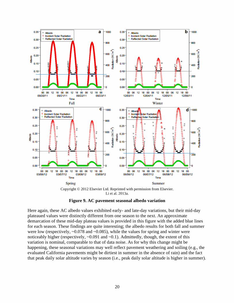
20


Li et al. 2013a.

Figure 9. AC pavement seasonal albedo variation

Here again, these AC albedo values exhibited early- and late-day variations, but their mid-day

plateaued values were distinctly different from one season to the next. An approximate

demarcation of these mid-day plateau values is provided in this figure with the added blue lines

for each season. These findings are quite interesting; the albedo results for both fall and summer

were low (respectively, ~0.078 and ~0.085), while the values for spring and winter were

noticeably higher (respectively, ~0.091 and ~0.1). Admittedly, though, the extent of this

variation is nominal, comparable to that of data noise. As for why this change might be

happening, these seasonal variations may well reflect pavement weathering and soiling (e.g., the

evaluated California pavements might be dirtiest in summer in the absence of rain) and the fact

that peak daily solar altitude varies by season (i.e., peak daily solar altitude is higher in summer).

21

It is not evident why these albedo variations were taking place. Perhaps the most obvious

possibility would be that the incoming solar insolation levels varied during periods of higher

(i.e., fall and summer) and lower (i.e., winter and spring) solar insolation levels. Even then, the

angle of incoming solar radiation throughout these various seasonal periods may also have had a

bearing on the resultant pavement albedo behavior.

Here again, it should be emphasized that this aspect of pavement albedo variability was not

considered to be an initial analytical factor during our project’s various site assessments.

Furthermore, the fact that our own city-level testing efforts were largely completed only during

summer periods was not conducive to further assessment of this behavior.

As shown in Figure 10, this sort of seasonal albedo variability has also been considered by Herb

et al. (2006) during a MnROAD-related pavement thermal modeling assessment. However, in

this case the authors applied a sinusoidal model to forcibly correct for albedo variations

connected with snow and ice pavement cover conditions.

Calibrated seasonal variation of surface albedo for Test Cell 33 in 2004

albedo=0.19+0.08×Cos(2π(cd+15)÷365), where cd is the calendar day

Prepared for MnDOT by the University of Minnesota St. Anthony Falls Laboratory.

Used with permission. Herb et al. 2006.

Figure 10. Theoretical seasonal albedo sinusoidal pattern

Another documented approach to considering albedo variability on a seasonal basis was

presented by Han et al. (2011) in conjunction with an asphalt pavement thermal modeling effort

and associated designation of optimized model albedo parameters at 29 different pavement

locations across the US. Table 4 identifies these parameters (i.e., where α˜ = albedo) and shows

that a number of northern location albedos were forced towards higher values (i.e., 0.35 in winter

versus 0.2 in summer). As explained by these authors, “[a]lthough the exact reason for the albedo

22

increase in the winter in the north is not clear, it seems that changes to the pavement surface,

associated with the snow coverage and freeze state in the winter, is likely.”

Table 4. Optimized model parameters

LTPP

section State

Summer Winter

α˜ ε εa ε−εa α˜ ε εa ε−εa

01–0101 Alabama 0.2 0.85 0.75 0.1 0.2 0.85 0.75 0.1

04–0215 Arizona 0.2 0.9 0.7 0.2 0.2 0.85 0.7 0.15

13–1005 Georgia 0.2 0.85 0.75 0.1 0.2 0.85 0.75 0.1

16–1010 Idaho 0.2 0.85 0.7 0.15 0.35 0.85 0.7 0.15

20–4054 Kansas 0.2 0.85 0.7 0.15 0.2 0.85 0.7 0.15

23–1026 Maine 0.2 0.8 0.75 0.05 0.3 0.8 0.75 0.05

27–1018 Minnesota 0.2 0.8 0.75 0.05 0.3 0.8 0.75 0.05

27–1028 Minnesota 0.2 0.8 0.75 0.05 0.3 0.8 0.75 0.05

28–1802 Mississippi 0.2 0.85 0.75 0.1 0.2 0.8 0.75 0.05

30–8129 Montana 0.2 0.9 0.7 0.2 0.35 0.85 0.7 0.15

31–3018 Nebraska 0.2 0.85 0.7 0.15 0.3 0.85 0.7 0.15

32–0101 Nevada 0.2 0.85 0.7 0.15 0.2 0.85 0.7 0.15

35–1112 New Mexico 0.2 0.85 0.7 0.15 0.2 0.85 0.7 0.15

36–4018 New York 0.2 0.9 0.75 0.15 0.35 0.85 0.75 0.1

37–1028 North Carolina 0.2 0.8 0.75 0.05 0.2 0.8 0.75 0.05

39–0901 Ohio 0.2 0.8 0.75 0.05 0.3 0.8 0.75 0.05

40–4165 Oklahoma 0.2 0.8 0.7 0.1 0.2 0.8 0.7 0.1

42–1606 Pennsylvania 0.2 0.9 0.75 0.15 0.3 0.85 0.75 0.1

46–9187 South Dakota 0.2 0.9 0.7 0.2 0.35 0.9 0.7 0.2

48–1068 Texas 0.15 0.85 0.7 0.15 0.15 0.85 0.7 0.15

48–1077 Texas 0.2 0.85 0.7 0.15 0.2 0.85 0.7 0.15

48–1122 Texas 0.15 0.85 0.75 0.1 0.15 0.85 0.75 0.1

48–3739 Texas 0.15 0.85 0.75 0.1 0.15 0.85 0.75 0.1

48–4142 Texas 0.15 0.85 0.75 0.1 0.15 0.85 0.75 0.1

49–3011 Utah 0.2 0.9 0.7 0.2 0.35 0.85 0.7 0.15

50–1002 Vermont 0.2 0.8 0.75 0.05 0.35 0.8 0.75 0.05

51–0113 Virginia 0.2 0.8 0.75 0.05 0.2 0.8 0.75 0.05

53–3813 Washington 0.2 0.85 0.75 0.1 0.35 0.85 0.75 0.1

56–1007 Wyoming 0.2 0.9 0.7 0.2 0.35 0.85 0.7 0.15

α˜=albedo, ε=mission coefficient (emissivity) of pavement, εa=absorption coefficient of pavement

Source: Han et al. 2011.

Original table Copyright © 2011 ASCE. All rights reserved.

23

While other factors may be in play, the simplest explanation is that (a) the sun never gets very

high in winter in northern latitudes, yielding a large incidence angle for the solar beam striking

the pavement, and (b) skies are often cloudy in winter, and diffuse light has an effective

incidence angle of about 60° (e.g., see Levinson et al. 2010a, which notes that the solar zenith

angle = 90° - solar altitude angle).

Albedo Multi-Year Variability

The existing literature offers relatively few publications that have considered, let alone

analytically examined, pavement albedo variation in relation to pavement aging. Indeed, only

five such papers have been published in the last two or more decades (see Table 2).

The first such assessment was reported by a research team working with the Lawrence Berkeley

National Laboratory’s Heat Island Group (Taha et al. 1992), and while the majority of this

presentation is focused on roofing materials, the authors mention that concrete pavements are

similarly prone to “weathering” and “aging.” The authors specifically cite new and old concrete

pavement albedo values of 0.33 and 0.22.

The second such report was presented by another research team affiliated with the Lawrence

Berkeley National Laboratory’s Heat Island Group (Pomerantz et al. 2005) and offers an

assessment of albedo measurements recorded at a number of asphalt pavements in San Jose,

California. Figure 11 depicts the resulting albedo-versus-age graph.

Used with permission. Pomerantz 2017.

Figure 11. AC pavement albedo aging

However, these researchers only presented their data, and no attempt was made to distill these

findings into a predictive analytical model.

The third assessment of age- and weathering-related pavement variation was published by Li and

Harvey in 2014. Figure 12 presents the authors’ findings over a limited eight-month period.

24

Used with permission. Li 2017.

Figure 12. Pavement albedo aging

Although limited by the short duration of the testing period, this paper does provide a brief

qualitative pattern for concrete and asphalt albedo during an eight-month period of weathering

exposure (i.e., where the albedo of asphalt tends to increase with time and that of concrete tends

to decrease).

The fourth assessment of pavement albedo variation in relation to long-term pavement aging was

published by Richard et al. in 2015. In this case, and as shown in Figure 13, these published

findings again include a graphed depiction of the albedo values measured at varying pavement

ages (i.e., from nearly new, early asphalt surfaces to two far older asphalt pavements at 27 and

32 years of age).

Copyright © 2015 ASCE. Used with permission from ASCE.

Richard et al. 2015.

Figure 13. Richard pavement albedo aging plot

25

Here again, as with the findings summarized above for Li and Harvey (2014), these results for

asphalt albedo variation show the same pattern of increase with continued aging. These authors

also took their findings to a further level of analytical evaluation, leading to their development of

the equation shown in the lower right corner of the chart in Figure 13 and below in Figure 14 as a

predictive logarithmic-based equation for asphalt albedo in relation to years of age.

Albedo=0.0133×ln(age)+0.1042

Copyright © 2015 ASCE. Used with permission from ASCE.

Richard et al. 2015.

Figure 14. Asphalt pavement albedo aging

The authors reported a coefficient of determination for their model’s fit of 0.6769 with their

analyzed data, which undoubtedly reflects the inherently limited set of data (i.e., nine points) that

they were evaluating.

The fifth assessment of age-related pavement albedo variation was completed as a Master’s

thesis at the University of Illinois by Sen in 2015 and includes both data presentation and a

predictive model. The following excerpt of Sen’s narrative commentary on the issue of age-

related pavement albedo variation is provided to fully capture his key technical points regarding

the current state of knowledge for pavement albedo variation and modeling:

The albedo of freshly paved asphalt has been measured to be 0.04 to 0.06, which rises to

0.09 to 0.18 after environmental aging. As noted, asphalt pavements initially have a very

low albedo, but with aging and aggregate exposure, it eventually increases significantly.

There has been little effort to understand how quickly this aging occurs and consequently,

most UHI studies assume a single, static value of albedo over the service life of the

asphalt pavement. Even the new [American Association of State Highway and

Transportation Officials (AASHTO)] (2011) pavement design guide recommends a

default value (static) of 0.15 for AC and 0.30 for PCC.

The albedo of a newly cast concrete pavement is higher than that of a new asphalt

pavement, at about 0.20 to 0.30. This albedo value is highly sensitive to the choice of

cement, aggregates, and supplementary cementitious materials, which can increase the

albedo of new concrete to 0.50 to 0.70. While carbonation initially increases the albedo

of concrete, it eventually decreases by about 0.06 to 0.19 because of weathering, soiling,

and abrasion. Thus, concrete albedo has the opposite trend to asphalt pavement with

higher albedo at construction and decreasing over time.

[…]

This paper reports the results of albedo measurements for a set of asphalt and concrete

pavement test sections of varying ages in Rantoul, IL. From the asphalt pavements, a

non-linear aging albedo model is proposed […].

Figure 15 depicts Sen’s chronologically organized set of albedo data values as well as a power-

function model for predicting asphalt pavement albedo relative to the local Illinois-based data

set.

26

— Model ▲ Data ■ Li et al. 2013a × Tran et al. 2009 ● Taha et al. 1992

Used with permission. Sen 2017.

Figure 15. Albedo aging data plot and model

Here again, this set of data is small, and it is noteworthy that this data pattern seems to suggest

an extremely rapid albedo increase (from ~0.12 when new to ~0.22+ within a space of only one

year). Sen’s own description of this change is as follows:

The functional form of the model implies that the pavement starts out at the at-

construction albedo and then undergoes weathering, with a majority of the weathering

effects taking place in the first few years and the rate of increase in albedo decreasing

over time.

PAVEMENT THERMAL PROPERTIES

Thermal Conductivity

The following guidance regarding pavement thermal conductivity values is offered in National

Cooperative Highway Research Program (NCHRP) Report 602: Calibration and Validation of

the Enhanced Integrated Climatic Model (EICM) for Pavement Design (Zapata and Houston

2008):

Dry Thermal Conductivity. Reasonable values of thermal conductivity for [hot-mix

asphalt (HMA)] pavements range from 0.44 to 0.81 BTU/(hr•ft•°F) [0.76 to 1.40

W/(m•°C)]. A default value of 0.67 BTU/(hr•ft•°F) [1.16 W/(m•°C)] was assumed for all

sections. For PCC pavements, the values range from 0.47 to 0.67 BTU/(hr•ft•°F) [0.81 to

1.16 W/(m•°C)]; a value of 0.57 BTU/(hr•ft•°F) [0.99 W/(m•°C)] was assumed. The dry

thermal conductivity of the unbound materials was not available in the database. The

EICM uses default values that are a function of the AASHTO soil classification. The

27

thermal conductivity default values were taken from Tye (1969), Larsen (1982), Yaws

(1997), and Farouki (1982).

These latter EICM default values correspond to recommended thermal conductivity values of

1.16 and 0.99 W/(m•°C) for AC and PCC pavements, respectively. The Table 5 summary

provides an additional set of similar published estimates for these values, which are also

comparable to the EICM recommendations.

Table 5. PCC and AC thermal conductivity value citations

Material

Thermal

Conductivity

(W/(m•°C)) Reference Source

Concrete (Stone) 1.7 Engineering ToolBox 2016a

Concrete (Medium) 0.4–0.7 Engineering ToolBox 2016a

Concrete (Dense) 1.0–1.8 Engineering ToolBox 2016a

Concrete (PCC) 0.99 Zapata and Houston 2008

Concrete (PCC) 1.5 Bentz et al. 2001, see Gui et al. 2007

Concrete (PCC) 1.719 Carlson et al. 2010

Concrete (PCC) 1.37–2.77 Khan 2002, see Carlson et al. 2010

Asphalt 0.75 Engineering ToolBox 2016a

Asphalt (HMA) 0.896 Carlson et al. 2010

Asphalt (HMA) 1.16 Zapata and Houston 2008

Asphalt (Dense fine grade) 1.21 Corlew and Dickson 1968, see Gui et al. 2007

Asphalt (Dense coarse grade) 2.00 Chadbourn 1998, see Gui et al. 2007

Asphalt 2.88 Xu and Solaimanian 2010

Asphalt (HMA) 0.8–1.6 Highter and Wall 1984, see Carlson et al. 2010

Specific Heat

The following guidance regarding pavement specific heat capacity values is offered in the

previously cited NCHRP report by Zapata and Houston (2008):

Heat Capacity. Reasonable values of heat capacity for HMA pavements range from 0.22

to 0.40 BTU/(lb•°F) [0.92 to 1.54 kJ/(kg•°C)]. A default value of 0.22 BTU/(lb•°F) [0.92

kJ/(kg•°C)] was assumed for all sections. For PCC pavements, the values range between

0.15 and 0.25 BTU/(lb•°F) [0.63 to 1.05 kJ/(kg•°C)]. A value of 0.15 BTU/(lb•°F) [0.63

kJ/(kg•°C)] was assumed. Soil heat capacities were not available in the [Long-Term

Pavement Performance (LTPP)] database. A recommended value of 0.18 BTU/(lb•°F)

[0.75 kJ/(kg•°C)] is used in the EICM for every material type (Robertson and

Hemingway 1995).

These latter EICM default values correspond to recommended specific heat capacity values of

0.92 and 0.63 kJ/(kg•°C) for AC and PCC pavements, respectively. The Table 6 summary

provides an additional set of similar published estimates for these values, which are also

comparable to the EICM recommendations.

28

Table 6. Published AC and PCC specific heat value citations

Material

Specific Heat a

(kJ/(kg•°C)) Reference Source

Concrete (Stone) 0.75 Engineering ToolBox 2016b

Concrete (Cast Lightweight) 1.0 Engineering ToolBox 2016b

Concrete (PCC) 0.63 Zapata and Houston 2008

Concrete (PCC) 1.0 Bentz et al. 2001, see Gui et al. 2007

Asphalt (HMA) 0.92 Zapata and Houston 2008

Asphalt 0.92 Engineering ToolBox 2016b

Asphalt (Dense fine grade) 0.921 Corlew and Dickson 1968, see Gui et al.

2007

Asphalt (Dense coarse grade) 0.866 Chadbourn 1998, see Gui et al. 2007

Asphalt 0.88 Xu and Solaimanian 2010

Emissivity

The Table 7 summary outlines the published literature that reports estimates for pavement

emissivity coefficient levels.

Table 7. Published AC and PCC emissivity value citations

Material

E

(dimensionless) Reference Source

Concrete (PCC) 0.88 Cengel 2003, see Gui et al. 2007

Concrete (Rough) 0.94 Cole-Parmer 2016

Concrete 0.94 Mikron Instrument Company n.d.

Concrete (Rough) 0.94 Engineering ToolBox 2016c

Asphalt 0.93 Engineering ToolBox 2016c

Asphalt 0.90–0.98 Mikron Instrument Company n.d.

Asphalt (Dense fine grade) 0.85 Cengel 2003, see Gui et al. 2007

Asphalt (Dense coarse grade) 0.85 Cengel 2003, see Gui et al. 2007

Density

The Table 8 summary outlines the published literature that reports estimates for pavement

density levels.

29

Table 8. Published AC and PCC pavement density value citations

Material

Density

(gm/cm3) Reference Source

Concrete 2.35 Bentz et al. 2001

Concrete (medium) 1.3–1.7 Engineering ToolBox 2016d

Concrete (high) 2.0–2.4 Engineering ToolBox 2016d

Asphalt (Fine grade) 2.238 Corlew and Dickson 1968, see Gui et al. 2007

Asphalt (Coarse grade) 2.1-2.4 RJC Solutions 2016

Asphalt (Dense grade) 2.15–2.5 RJC Solutions 2016

Asphalt (Dense grade) 2.1 Chadbourn 1998, see Gui et al. 2007

Soil (Dry) 1.5 Cengel 2003, see Gui et al. 2007

Heat Flux

The Table 9 chronological summary outlines the published literature regarding pavement heat

flux analysis and assessment.

Table 9. Chronological pavement heat flux testing and assessment publications

Date Authors Notes

1996 Asaeda et al. 1996 Used Eko MF-81 heat flux sensor

2000 Asaeda and Ca 2000 Used Eko MF-81 heat flux sensor

2012 Takebayashi and

Moriyama 2012

Used Kipp & Zonen CPR-CNR1 downward and upward

pyranometers and Eko MR-180M heat flow sensors (Note

that both asphalt and concrete surfaces were evaluated.)

2013 Li et al. 2013a Used NovaLynx Corp. Mdl. 240-8140 dual-Up-down

pyranometer; calculated (but not measured) heat flux

2014 Kertesz and Sansalone

2014

Only heat flux model analysis

2014 Qin and Hiller 2014 Only heat flux model analysis

2015 Hendel et al. 2015 Used Taylor heat flux flowmeter

2015 Li and Harvey 2014,

Li et al. 2015

Used NovaLynx Corp. Mdl. 240-8140 dual-up-down

pyranometer; calculated (but not measured) heat flux

2015 Garcia et al. 2015 Used ITI Mdl. GHT-2C geothermal heat flux transducer

2016 Zhang et al. 2015 Used Hukseflux Mdl. HFP01SC-10

2016 Hassn et al. 2016 Used ITI Mdl. GHT-2C geothermal heat flux transducer

PAVEMENT THERMAL MODELING

A general chronologically sorted synopsis of published pavement thermal modeling efforts is

provided in Table 10.

30

Table 10. Chronology of pavement thermal modeling publications

Date Author(s) Notes

1953 Vehrencamp 1953 Early classic modeling effort with air-earth system, which can

be extrapolated to pavement systems

1968 Corlew and Dickson 1968 Early classic modeling effort; asphalt pavement focus

1985 Dempsey et al. 1985 Seminal publication leading to original MEPDG thermal model

1993 Lytton et al. 1993 Genesis of the integrated climate effects model for pavements

1993 Solaimanian and Kennedy

1993

One-dimensional steady state model

1993 Asaeda and Ca 1993

1996 Asaeda et al. 1996

1997 Taha 1997

2000 Asaeda and Ca 2000 Highly cited publication (14 citations)

2000 Van Buren et al. 2000

2001 Hermansson 2001 Swedish publication; raised “strong questions” about Superpave

maximum pavement temperature calculation

2002 Yavuzturk and Ksaibati

2002, Yavuzturk et al. 2005

Asphalt pavement focus; highly cited publication (18 citations)

2005 Yavuzturk et al. 2005 Asphalt pavement focus; two-dimensional finite difference

2005 Minhoto et al. 2005 Asphalt pavement focus; three-dimensional finite element

method

2005 Sansalone and Teng 2005 One-dimensional heat transfer and surface temperature model

2006 Herb et al. 2006 One-dimensional finite difference

2007 Gui et al. 2007 Highly cited publication (18 citations)

2008 Thompson et al. 2008

2008 Kim et al. 2008

2008 Marasteanu et al. 2008 One-dimensional finite difference model

2009 Ho and Romero 2009 One-dimensional finite element method

2009 Herb et al. 2009 One-dimensional heat transfer and surface temperature model

2011 Qin and Hiller 2011 One-dimensional finite difference

2011 Wang 2011 Transient conduction with sinusoidal boundary temperature at

the upper pavement surface approximating daily cycle of solar

radiation

2012 Hall et al. 2012, Mohseni

1998

One-dimensional finite difference

2014 Kertesz and Sansalone 2014 One-dimensional heat transfer

2014 Qin and Hiller 2014 One-dimensional transient heat transfer

2014 Alavi et al. 2014 Finite control volume model

2015 Sen 2015 Used ILLI-THERM model, based on transient heat flow

Solaimanian and Kennedy (1993) developed a rather simple approach using maximum air

temperature and hourly solar radiation as climatic inputs while using a one-dimensional steady

state model for the conduction problem. This approach led to a computationally efficient solution

and produced accurate predictions for maximum surface temperature, which was the intended

31

purpose. The surface temperature results were then used to predict the coincident temperature at

depth by curve fitting empirical data. The resulting semi-empirical solution is appealing because

of its simplicity, but it is of limited utility because the method only applies to peak surface

temperature conditions.

Most investigators have chosen to use a transient numerical model for the conduction problem,

with the most common being a one-dimensional finite difference scheme (Hermansson 2001,

Gui et al. 2007, Herb et al. 2006, Herb et al. 2009, Qin and Hiller 2011, and Hall et al. 2012).

One-dimensional finite element (Ho and Romero 2009), two-dimensional finite difference

(Yavuzturk et al. 2005), and three-dimensional finite element (Minhoto et al. 2005) approaches

have also been applied to the problem. The two-dimensional and three-dimensional methods add

significant computational complexity but have not been shown to increase predictive accuracy.

In each case, the upper boundary condition for the conduction problem is a heat flux that results

from a surface energy balance. However, the lower boundary condition has been investigated

with significantly different approaches. Hermansson (2001) used a constant temperature of 12 °C

for the lower boundary condition at a depth of 5 m. This assumption was used regardless of

geographic location or time of year. Gui et al. (2007) used a lower boundary condition of 33.5 °C

at a depth of 3 m, which was measured at the site of the model confirmation experiments in

Arizona. Hall et al. (2012) also use an isothermal lower boundary at a depth of 2 m but do not

specify the value used. Herb et al. (2006 and 2009) uses an adiabatic boundary at a depth of 10 m

for the lower boundary condition. Qin and Hiller (2011) tried to account for the fact that the earth

is continuously cooling by applying a constant vertical temperature gradient of 0.03 °C/m at a

depth of 20 m. The EICM uses an isothermal boundary that varies with location. The depth for

this lower thermal boundary is not specified, but Lytton et al. (1993) state that 3.7 m is typical.

SUSTAINABILITY RATING SYSTEMS RELATIVE TO ALBEDO PROPERTIES AND

COOL PAVEMENT ISSUES

When this project was initiated in August 2012, more than a dozen sustainable highway and

horizontal infrastructure rating systems had been developed and were in use in the United States.

The goals of these rating systems were comparable to those of the earlier (circa late 1990s)

Leadership in Energy and Environmental Design (LEED) initiative, which had been established

for building systems (i.e., vertical versus horizontal infrastructure). As was the case with LEED’s

approach to awarding points for building features that would advance sustainability outcomes

(including LEED’s consideration of cool non-roof surfaces), several of these sustainable

highway rating systems had similar levels of focus on a similar “cool pavement” goal.

Table 11 provides a synopsis of the most popular versions of the sustainable infrastructure

methods in existence before the middle of 2012. The systems’ respective considerations of

pavement albedo properties and effects in relation to heat islands, cool pavements, or localized

increased air temperature are addressed.

32

Table 11. Sustainability highway infrastructure rating systems and cool pavement aspects

Rating

System

Responsible Agency

and Approximate

Genesis Year Cool Pavement Aspect

Total

Points

Cool

Pavement

Points

Percentile

“Cool

Pavement”

Effects

AASHTO

Sustainability

Highway

Checklist

AASHTO ~2005 None N/A N/A N/A

GreenLITES NYSDOT ~2008 “S-2h: Site materials selection and detailing to

reduce overall urban ‘heat island’ effect”

273 1 0.4%

ASCE-SIPRS American Society of

Civil Engineers

~2009

“Avoid heat islands. Does the design avoid the

creation of heat islands?”

1000 10 1%

I-LAST Illinois DOT ~2009 “Reduce urban heat island effect” 219 1 0.5%

GreenPAVE Ontario Ministry of

Transportation (Canada)

~2010

“Cool Pavements” 36 2 5.6%

Greenroads University of

Washington and

CH2MHILL ~2010

“Reduce contribution to localized increased air

temperatures due to pavement reflectance and

minimize stormwater runoff temperatures”

“Use a pavement surface with a minimum

albedo of 0.3 (measured using ASTM E903)

for a minimum of 50% of the total project

pavement surfacing by area”

218 5 2.3%

INVEST FHWA ~2012 A “cool pavement” factor reportedly not

included by FHWA “pending further research”

N/A N/A N/A

33

The first and last of these chronologically sorted options (including the FHWA’s circa 2012

Infrastructure Voluntary Evaluation Sustainability Tool [INVEST] and AASHTO’s circa 2005

“checklist”) do not list an albedo-related sustainability scoring factor. However, the remaining

five of these systems all considered the effect of a pavement’s thermal behavior at percentile

levels (i.e., relative to the rating system’s summary score) ranging from ~5.6% to ~0.4%.

Of these latter five options, four of them (i.e., GreenPAVE, the American Society of Civil

Engineers (ASCE) Sustainable Infrastructure Project Rating System (SIPRS), I-LAST, and

GreenLITES), considered and scored the pavement “albedo” factor on a qualitative basis, with 1

to 10 points allocated for projects where pavement coolness and/or reduced urban heat island

effects were considered.

The 2012-era version of the Greenroads rating system was unique in that it was the only

sustainable infrastructure rating system that applied a quantitative approach to pavement albedo,

stipulating that one-half or more of a project’s paved surface area must use a material with a

minimum 0.3 albedo value. This quantitative approach for Greenroads was likely influenced by

LEED’s consideration of, and one-point allocation for, the “heat island effect” for “non-roof”

surfaces (see LEED-NC-v2.2 SSc7.1: Heat Island Effect—Non-Roof), which included the

following optional sustainability-focused one-point allocation parameters:

• Option 1: Non-Roof Hardscape Surfaces: Light-colored surfaces with high solar reflectance

index (SRI > 29).

• Option 1: Onsite Parking: Any parking area roof must have an SRI > 29, be covered by solar

panels, or be vegetated.

An important aspect that must be highlighted for all of the highway infrastructure sustainability

rating systems as of August 2012, including that of LEED (i.e., prior to LEED v4), is that none

of these methods considered the fact that the reflectivity of pavement or non-roof surfaces would

change over time as these surfaces age.

34

CHAPTER 4. PAVEMENT THERMAL MODELING

PAVEMENT THERMAL DYNAMICS

Applying the science and engineering of heat transfer to pavements involves a set of terminology

that is not commonly understood or applied in the highway community. At the same time, many

of the pavement and materials terms used by highway engineers have subtle differences from

these terms’ meaning and usage in other disciplines that would not be fully understood by

thermal dynamic experts. For this report, it is critical that a consistent but simple set of thermal

and pavement terms is used. Table 12 provides the terms and their general definitions.

Table 12. General summary of pavement thermal terms and symbols

Terms Description Symbol [units]

Solar radiance Incident (downwelling) solar power per unit area;

also called insolation

q"solar[W/m2]

Albedo Fraction of solar irradiance that is reflected; also

called solar reflectance

R[dimensionless]

Reflected radiance Reflected (upwelling) solar power per unit area R×q"solar[W/m2]

Solar heat gain Absorbed solar radiance q"abs=(1-R) ×

q"solar[W/m2]

Thermal radiation Net thermal infrared (a.k.a., far infrared) power per

unit area radiated from surface to its environment;

also known as thermal radiative heat flux

q"rad[W/m2]

Convection Power per unit area convected from surface to air;

also known as convective heat flux

q"conv[W/m2]

Conduction Power per unit area conducted through a body; also

known as conductive heat flux

q"cond[W/m2]

Thermal

conductivity

Coefficient relating conductive heat flux (power

per unit area) to temperature gradient

K[W/(m•°C)]

Specific heat at

constant pressure

Heat energy required to raise by one unit the

temperature of a unit of mass

cp[J/(kg•K)]

Cement concrete

pavement

Pavement in which the aggregate is bound with

cement

PCC

Asphalt concrete

pavement

Pavement in which the aggregate is bound with

asphalt (bitumen)

AC

Composite

pavement

Pavement with layers of both cement concrete and

asphalt concrete, most commonly asphalt concrete

over cement concrete

Aggregate base Layer of aggregate below the pavement

Subbase Layer below the base with better material

properties than the natural subgrade; typically

defined in this report as “subgrade”

Subgrade Natural occurring soils below the pavement

structure, most commonly fine-grained sands, silts

and clays

35

The basic components of the pavement thermal model are shown in Figure 16.

Figure 16. Basic thermal model (day)

While solar radiation is the primary source of energy entering the modeled system, a pavement

also exchanges heat with the air and sky. For example, even if the pavement were fully shaded, it

should warm up over the course of the day as the outside air temperature rises.

The pavement surface reflects a portion of the solar radiation away from the pavement, and the

balance is absorbed into the pavement. A portion of the absorbed energy is radiated back out of

the pavement, another portion is convected from the surface, and the balance is conducted into

the materials below the pavement surface. As the thermal energy is conducted down, each layer

stores a portion of the energy, and the balance is conducted deeper until all the energy is stored.

Pavement thermal dynamics are just that—dynamic—and extend across both day and night

periods. The above description of heat flow applies to daylight hours, while at night the solar

radiation pathway is not present. Figure 17 shows the nighttime transformation of the surface

radiation, surface convection, and conduction and storage processes.

36

Figure 17. Basic thermal model (night)

Generally, a portion of the energy stored in the pavement during the daytime hours is released

from the pavement surface at night. In addition to this daily cycle, the pavement thermal

response transitions as the pavement is exposed to the annual climate cycle. Within any given

24-hour cycle, though, the net heat energy stored in a body during a given interval may be

positive, negative, or zero. The following sections discuss pavement thermal dynamics in more

detail.

PAVEMENT ALBEDO MODELING BACKGROUND

As shown in Figure 16, when sunlight strikes the pavement, some of the radiation is reflected

back into the air while the remaining radiation is absorbed by the pavement structure. While the

absorbed radiation can be used to aid in developing thermal models for pavement structures, a

pavement’s albedo is designated as the solar reflectance or the fraction of solar irradiance that is

reflected (as a dimensionless value between 0 and 1). Figure 18 illustrates the basic concept of

albedo.

Figure 18. Basic albedo model

It has been suggested through modeling that increasing pavement albedo could reduce energy

costs and reduce smog-related medical and lost-work expenses (Silva et al. 2009). Other work

has shown that increasing pavement albedo could decrease a pavement’s peak summertime

temperatures (Brown et al. 2005) or decrease peak energy demands for major cities (Harvey et

37

al. 2011). But while people have postulated about the potential benefits of high-albedo

pavements and some states and cities have already begun to request their use (Oleson et al.

2010), the mechanisms that control albedo have not been adequately modeled and characterized

for pavement structures. Based on past literature, improved modeling for characterizing

pavement heat transfer would need to incorporate characteristics such as pavement materials,

age, and environmental effects.

Much of the current literature within and outside of the realm of pavements links albedo to color

and does not investigate further into material properties. For example, one might state that if

frost or snow is covering a pavement, the lightly colored surface will increase the albedo by

reflecting more of the shortwave radiation (Hermansson 2001). Even then, however, one should

also consider that the ice or snow may have a different texture or inherent capability to reflect

irrespective of color.

Although pavements have albedos that are generally expected to map well to lightness, it is

worth noting that this correlation does not apply in the case of building envelope materials.

Indeed, for the past several decades it has been understood that color does not necessarily predict

albedo. Section 1 of Levinson et al. (2005b) and Section 2 of Levinson et al. (2007) provide

further clarification on this point.

Therefore, one of the critical components of modeling a pavement’s albedo is understanding the

materials that compose the pavement. General pavement albedo values, as identified in a widely

cited publication developed by the Lawrence Berkeley National Laboratory research group

(Pomerantz et al. 2005), appear to fall within the following ranges: 0.04 to 0.16 for AC and 0.18

to 0.40 for PCC. Most of these albedo values are tied to the color of the pavement, whether

asphalt (black) or concrete (gray or white).

However, the matter is more complicated than just linking pavement albedo to pavement type. A

69-week albedo study using 32 different concrete mixtures that incorporated a variety of

cements, sands, and rocks was conducted at the Lawrence Berkeley National Laboratory. During

this study, 10 readings from an SSR were used to quantify the albedo of the different concrete

mixtures. For a mature concrete that has not undergone environmental exposure, weathering,

abrasion, etc., the concrete’s albedo correlates strongly to the albedo of the cement and sand

chosen for its mixture design (e.g., see Figure 19, which is reproduced from Levinson and

Akbari 2002).

38


Levinson and Akbari 2002.

Figure 19. Properties of mature, unexposed concrete.

39

It should also be noted that Marceau and VanGeem (2007) conducted similar testing with an

even wider variety of components and better fabrication methods for the tested concrete

specimens. The New York City Department of Design and Construction even lists using lightly

colored aggregates or chip seals (i.e., exposed aggregate on asphalt binder) to increase pavement

albedo (Oleson et al. 2010).

Additionally, pavement color can be influenced by material choice. Concrete can be a gray or

white color depending on the type of cement chosen for the mixture, and various other additives

(notably fly ash and slag) can have further effects on overall concrete color and reflectivity (e.g.,

see Figure 20, which is reproduced from Marceau and VanGeem 2007).

Used with permission. ©Portland Cement Association 2007.

Figure 20. Cementitious material color variation

An Arizona State University (ASU) study further showed the need to look at the properties of the

materials used in the pavement layer when comparing pavement albedo and pavement surface

temperature and showed that parameters such as pavement material thickness, white painting,

and even inclusion of rubber in both concrete and asphalt can affect pavement albedo (Figure

21). There is an obvious trend demonstrated by this figure’s correlation between albedo and

temperature results, with lower albedo pavements showing lower maximum surface

temperatures.

40

Used with permission as modified from the Portland Cement Association ©2008. Kaloush, et al. 2008.

Figure 21. Surface temperature and albedo for selected types of pavements in Phoenix,

Arizona

It has been stated that while the color of the binder is important, if an asphalt pavement were to

use a lightly colored aggregate, the pavement might appear light in color and reflect more solar

radiation (Kinouchi et al. 2004).

While some agencies and studies focus on just the color of the binder and aggregate, other

researchers (see Figure 22) have investigated the use of high-albedo paint coatings on pavements

to increase albedo (Cambridge Systematics, Inc. 2005, Wan et al. 2009).

Max

imu

m S

urf

ace

Tem

per

atu

re (

oC

)

Max

imu

m S

urf

ace

Tem

per

atu

re (

oF)

Albedo

Max

imu

m S

urf

ace

Tem

per

atu

re (

oF)

Asphalt RubberThick

Asphalt RubberThin

Chip Seal StandardHot Mix Asphalt Thin

Crumb-RubberConcrete

Asphalt Rubber Thinwith White Paint

Hot Mix Asphalt Thick

Asphalt Rubber Thinwith White Paint

PCC Concrete12-inch

Asphalt Rubber Thickwith White Paint

Hot Mix Asphalt Thickwith White Paint

PCC Concrete

30-cm

41

Used with permission. Kinouchi et al. 2004.

Figure 22. Paint-coated asphalt pavement

The study by Kinouchi et al. (2004) investigated the use of an innovative paint coating

technology that was used to increase the albedo of a conventional asphalt pavement without

changing the color. This material worked by allowing the near infrared spectrum to be highly

reflected while still having low reflectivity for the visible spectrum. The second study

investigated a dark-colored pavement coating named “PerfectCool,” which was developed by

NIPPO Corporation Ltd., Japan. On-site measurements showed that while this material was

darkly colored, its chemical and physical properties allowed it to reflect almost 81% of the near

infrared radiation and reduce the pavement temperature by between 16 and 38 °C (Wan et al.

2009).

In the previously mentioned Lawrence Berkeley National Laboratory study (Pomerantz et al.

2005), weathering, abrasion, soiling, and wetting of the concrete specimens all reduced the

albedo of the concrete pavement. As previously mentioned, the albedo of a concrete is highly

correlated to the albedo of its cement and sand (Marceau and VanGeem 2007); however, as

weather and traffic removes the thin layer of paste from the surface of the pavement, the albedo

of the concrete becomes more closely related to that of its aggregate source (Levinson and

Akbari 2002).

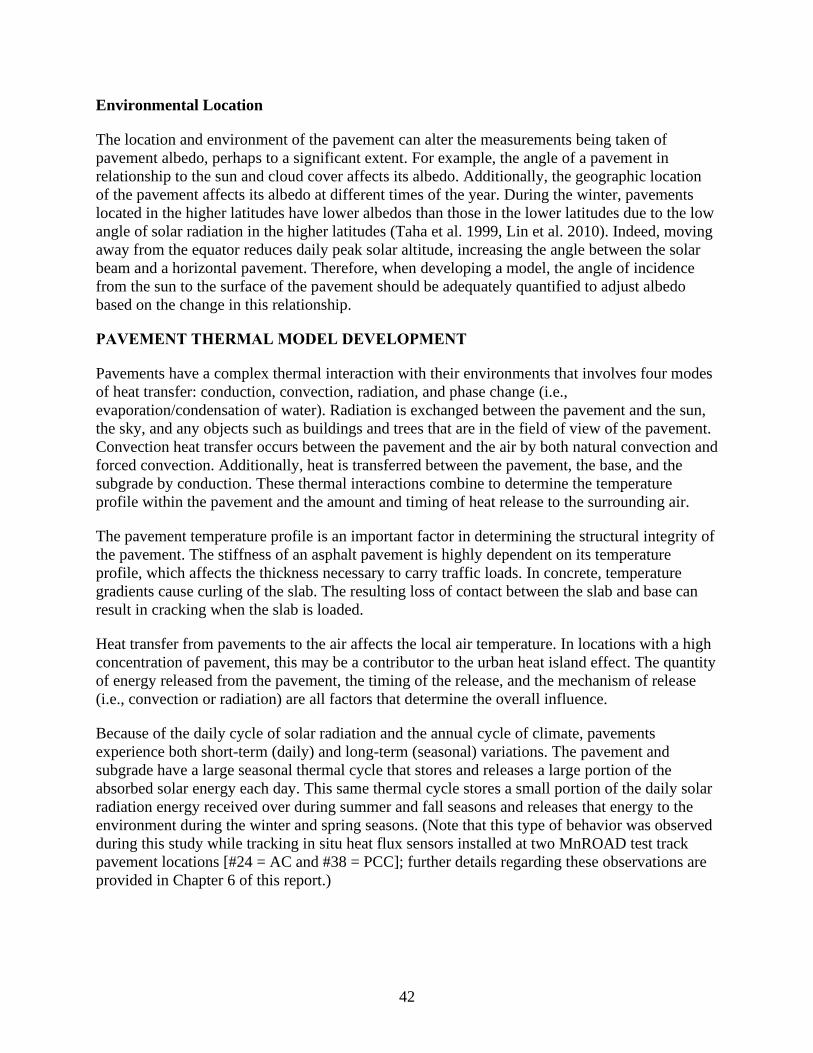
42

Environmental Location

The location and environment of the pavement can alter the measurements being taken of

pavement albedo, perhaps to a significant extent. For example, the angle of a pavement in

relationship to the sun and cloud cover affects its albedo. Additionally, the geographic location

of the pavement affects its albedo at different times of the year. During the winter, pavements

located in the higher latitudes have lower albedos than those in the lower latitudes due to the low

angle of solar radiation in the higher latitudes (Taha et al. 1999, Lin et al. 2010). Indeed, moving

away from the equator reduces daily peak solar altitude, increasing the angle between the solar

beam and a horizontal pavement. Therefore, when developing a model, the angle of incidence

from the sun to the surface of the pavement should be adequately quantified to adjust albedo

based on the change in this relationship.

PAVEMENT THERMAL MODEL DEVELOPMENT

Pavements have a complex thermal interaction with their environments that involves four modes

of heat transfer: conduction, convection, radiation, and phase change (i.e.,

evaporation/condensation of water). Radiation is exchanged between the pavement and the sun,

the sky, and any objects such as buildings and trees that are in the field of view of the pavement.

Convection heat transfer occurs between the pavement and the air by both natural convection and

forced convection. Additionally, heat is transferred between the pavement, the base, and the

subgrade by conduction. These thermal interactions combine to determine the temperature

profile within the pavement and the amount and timing of heat release to the surrounding air.

The pavement temperature profile is an important factor in determining the structural integrity of

the pavement. The stiffness of an asphalt pavement is highly dependent on its temperature

profile, which affects the thickness necessary to carry traffic loads. In concrete, temperature

gradients cause curling of the slab. The resulting loss of contact between the slab and base can

result in cracking when the slab is loaded.

Heat transfer from pavements to the air affects the local air temperature. In locations with a high

concentration of pavement, this may be a contributor to the urban heat island effect. The quantity

of energy released from the pavement, the timing of the release, and the mechanism of release

(i.e., convection or radiation) are all factors that determine the overall influence.

Because of the daily cycle of solar radiation and the annual cycle of climate, pavements

experience both short-term (daily) and long-term (seasonal) variations. The pavement and

subgrade have a large seasonal thermal cycle that stores and releases a large portion of the

absorbed solar energy each day. This same thermal cycle stores a small portion of the daily solar

radiation energy received over during summer and fall seasons and releases that energy to the

environment during the winter and spring seasons. (Note that this type of behavior was observed

during this study while tracking in situ heat flux sensors installed at two MnROAD test track

pavement locations [#24 = AC and #38 = PCC]; further details regarding these observations are

provided in Chapter 6 of this report.)

43

This latter cyclic thermal imbalance is a transient (i.e., time varying) heat transfer problem that

requires mathematical models for each of the modes of heat transfer. The modes of heat transfer

are as follows:

• Conduction (beneath the surface).

• Convection (from the surface).

• Solar absorption.

• Radiative cooling.

Furthermore, a fifth transient factor involving water evaporation and condensation (i.e., water

phase change) needs to be added for those periods when the pavement, base, and subbase

materials are not dry. The modeling challenge presented by this behavior, though, is extremely

difficult, to the point that no such model currently exists.

Analytical solutions of the transient conduction problem have been presented (Liu and Gazis

2001, Wang 2011) by assuming a sinusoidal boundary temperature at the upper surface of the

pavement to approximate the daily cycle of solar radiation. This approach is useful for showing

the characteristic response of the pavement but requires that the pavement surface temperature be

a function of time as an input boundary condition. Because the surface temperature is not usually

available as input data, this approach is not particularly useful for solving the larger thermal

interaction problem.

The results of short duration modeling of just a few days are relatively insensitive to the lower

boundary condition or the depth at which it is applied, and all investigators are able to predict

pavement temperature to within 3 to 5 °C with their respective assumptions. Modeling for long

periods of time would require more careful attention to the lower boundary condition because of

the long-term storage of energy at depth, which tends to build up over time. This is evidenced by

the results of Gui et al. (2007), where the assumed initial condition for the model was a constant

temperature of 33.5 °C from the surface of the pavement to the depth of 3 m. Daily heat cycles

were repeated to precondition the subgrade thermal storage before modeling a three-day run of

experimental data. These predictions matched the experimental data very well after 10

preconditioning cycles but became progressively less accurate after 20 and 30 preconditioning

cycles.

The convective heat flux from a pavement surface (q"conv) is typically modeled, as shown in

Figure 23, using Newton’s Law of Cooling.

q"conv=h×(Ts-Tair)

Figure 23. Convective heat transfer

Where:

q"conv = the convective heat transfer per unit area from the surface to the air (W/m2).

h = the convective heat transfer coefficient (W/(m2•K)).

Ts = the surface temperature (K).

Tair = the air temperature far away from the surface (K).

44

However, the method for arriving at the value of h is varied and inherently tricky because it is

difficult to know where the momentum and thermal boundary layers began. Indeed, there are

many possible models for determining the convective heat transfer coefficient. Solaimanian and

Kennedy (1993) simply assigned a constant value of 3.5 W/(m2•°C) for h regardless of wind

speed or the temperature difference between the pavement and the air. Gui et al. (2007) used a

correlation for laminar flow over a flat plate, which assumes simultaneous development of the

hydrodynamic and thermal boundary layers and ignores natural convection. Yavuzturk et al.

(2005) adopted a flat plate correlation (allowing for transition from laminar to turbulent flow) for

forced convection but added a flat plate correlation for natural convection. The final choice of

convective coefficient h was taken as the larger of the natural and forced convection coefficients.

Qin and Hiller (2011) also used a laminar flat plate correlation but with the addition of a constant

(5.6 W/(m2•°C)) to account for natural convection. Several authors (Hermansson 2001, Ho and

Romero 2009, Herb et al. 2006) used some variation of the empirical Vehrencamp (1953) model,

where the value of h is given by the equation in Figure 24.

h=698.24[0.00144×Tm0.3×U0.7+0.00097×(Ts-Tair)

0.3]

Figure 24. Convective heat transfer coefficient h derivation

Where:

Tm = the average of the surface temperature and the air temperature (K).

U = the wind speed (m/s).

The EICM also uses the Vehrencamp model, but the value of h is capped at 17 W/(m2•°C) to

prevent numerical instability in the conduction model. Hall et al. (2012) used the equation in

Figure 25 to calculate the convective coefficient based on the best fit of pavement temperature

data from multiple sites.

h=5.8+4.1U

Figure 25. Convective heat transfer coefficient simplification

It should be noted that several parameters in Hall et al. (2012) were manipulated simultaneously

to achieve the best fit for the limited experimental data set, so the fundamental basis for this

choice is relatively weak.

The Vehrencamp model seems to be the most realistic model for a number of reasons. This

model is based on the empirical correlation of experimental data obtained from a large dry

lakebed in California and thus models convection from a flat surface where the hydrodynamic

boundary layer is highly developed. This scenario matches the physical situation for convection

from pavements better than the flat plate correlations, which assume simultaneous development

of the hydrodynamic and thermal boundary layers. Also, the Vehrencamp model allows for

contributions from both forced and free convection.

In the equation in Figure 24, the first term inside the brackets is the forced convection

contribution, and the second term inside the brackets is the free convection term. The structure of

the forced convection term suggests that it is largely modeling turbulent flow, which is expected

given the high degree of hydrodynamic boundary layer development.

45

There are some aspects of convection from pavements that do not match well with the

Vehrencamp model. Because pavements typically have a higher surface temperature than other

upwind surfaces, a new thermal boundary layer would be expected to develop at the leading edge

of the pavement.

In contrast, the Vehrencamp model is developed for a large isothermal surface, and the thermal

boundary layer would already be highly developed similarly to the hydrodynamic boundary

layer. The effect of this physical difference would be an underprediction of the heat transfer from

pavements. Also, it should be noted that the wind speed used by Vehrencamp is based on

measurements made at an elevation of 2 m. Often the Vehrencamp model is used with weather

station data, where the standard is to measure the wind speed at an elevation of 10 m. Because

wind speed decreases with elevation, using wind speed data taken at 10 m in the Vehrencamp

model would tend to over-predict the heat transfer rate. The air temperature measurement in the

Vehrencamp model is at a height of 2 m, which matches well with the standard for weather

stations.

The radiative exchange to and from pavements occurs in two distinct wavelength bands. Solar

radiation is virtually all at short wavelengths (UV, visible, NIR), where 99% of terrestrial

sunlight arrives in the spectrum of 300 to 2500 nm, and radiation between the surface and the sky

is at long wavelengths (far infrared). At a given wavelength, the absorptivity of a surface is equal

to the emissivity. However, both are a function of wavelength for a given surface. Therefore,

adequately modeling radiative exchange for pavements requires two models: one for absorption

of solar radiation and one for radiative cooling. Even if the pavement were “black” (i.e.,

completely absorbing) at all wavelengths, exchange of longwave (thermal) radiation would still

need to be treated differently than exchange of shortwave (solar) radiation because the pavement

emits only longwave radiation.

Short wavelength radiation from the sun impinging on the pavement is a function of time of day,

time of year, latitude, orientation of the pavement, and various atmospheric factors such as cloud

cover. Part of the solar radiation is reflected from the surface back into space, and part is

absorbed by the surface. A comprehensive review of models to predict solar radiation falling on

a surface is given by Wong and Chow (2001). Most pavement thermal models have used

measured (as opposed to predicted) solar radiation, and there is general agreement among

investigators as to how those data are used. If the solar irradiance (qsolar, the solar power per unit

area) is known, then the solar energy absorbed by the pavement (qabs) is given by the equation in

Figure 26

q"abs=(1-R)×q"solar

Figure 26. Absorbed solar energy

Where:

R = the solar reflectance (albedo) of the surface.

q"solar = the solar insolation heat transfer per unit area (W/m2).

The surface of the pavement also exchanges long wavelength radiation with the sky and any

surfaces that are in the field of view of the pavement. In the case of radiative exchange with only

46

the sky, the temperature of both the pavement and the sky as well as the emissivity of the

pavement must be known. The radiative heat transfer from the pavement to the sky (q"rad) is

calculated as shown in Figure 27.

q"rad=E×σ×(Ts 4-Tsky

4)

Figure 27. Radiative energy transfer

Where:

E = the thermal emittance of the surface (i.e., emissivity).

σ = the Stefan-Boltzmann constant (5.67×10-8 W/(m2•K4)).

Ts = the surface temperature (K).

Obtaining an effective sky temperature (Tsky) model has been the subject of several studies. One

simple approach, albeit not recommended, simply approximates Tsky as being equal to the air

temperature, Tair (Hermansson 2001). However, most investigative efforts to produce an accurate

but simple model for the clear sky radiative environment include some factor to account for

water vapor (e.g., Berdahl and Fromberg 1982). Hall et al. (2012) give a review of several

models for Tsky but settle on the empirical Bliss equation based on the best fit of experimental

data for pavement thermal modeling. The Bliss equation estimates Tsky as shown in Figure 28.

Tsky=Tair(0.8+0.004Tdp)0.25

Figure 28. Background sky temperature derivation

Where:

Tsky and Tair = the sky and air temperatures , respectively (K).

Tdp = the dew point temperature (°C).

This equation has also been used by Yavuzturk et al. (2005), Gui et al. (2007), and the American

Society of Heating, Refrigerating, and Air-Conditioning Engineers (ASHRAE 2003).

It should be noted that the preceding derivations used for quantifying the absorptive, conductive,

convective, and radiative heat transfer pathways do not include a “water phase change” pathway.

The presented model has a degree of error because it does not account for the presence of

moisture in the pavement, base, and subbase materials. Three factors influenced the decision not

to include the water-related heat transfer pathway. First, the level of effort required to accurately

measure the in situ presence and state of water within pavement, base, and subbase materials

exceeded what could be realistically achieved during this study. Second, the assumption that the

pavement system being modeled is dry and non-frozen (and consequently has no evaporation,

condensation, or freezing mechanisms) allows for a scenario where the model would predict the

highest possible pavement temperatures. This “hottest-case” scenario is of great importance for

pavement design and performance. Third, the complexity of modeling required to accurately

track water-related energy exchange within a pavement system is significantly greater than for

the other heat transfer pathways (i.e., absorptive, conductive, etc.). This amount of model

development was beyond this project’s capacity to provide this higher level of modeling

accuracy.

47

A user guide for the Microsoft Excel-based pavement thermal model created during this study is

provided in Appendix B. In addition, a sample spreadsheet model is provided in the spreadsheet

file at https://cptechcenter.org/research/completed/quantifying-pavement-albedo/.


48

CHAPTER 5. METHODOLOGY

GENERAL WORK PLAN

The testing plan for this study was divided to support the development of both the albedo model

and the thermal model. The primary data for the albedo model were collected from seven distinct

sites around the country. The primary sources of data for the thermal model were the MnROAD

and NCAT test tracks. The testing plan was also integrated with numerous features to maintain a

high level of data quality and security. The primary testing plan for the albedo model was to

collect data from 10 locations at each of 7 sites. Figure 29 provides a visual perspective of the

originally planned general distribution of field test sites within regions spread across the US.

Figure 29. City-level field testing plan

The intended testing window was narrowly defined to collect data in the summer month period,

during midday, on days with no cloud cover, and in dry pavement conditions (in the last 24

hours). The key controlled variables for the study were pavement type, pavement age, aggregate

color, and solar angle. Other variables to be measured included aggregate silica content and

pavement surface texture. The research team subsequently planned to collect the following

information at all seven city test locations:

• Solar energy.

• Solar angle to the pavement surface.

• Pavement surface reflectivity.

• Pavement temperature gradient (i.e., only on the pavement).

• Pavement surface emissivity (at 2 of the 10 locations in each city).

• Pavement materials (base and subgrade) (from agency records).

• Ambient air temperature (at 2 of the 10 locations in each city).

• Ambient humidity (at 2 of the 10 locations in each city).

• Pavement type (via visual inspection).

• Pavement aggregate color (via visual inspection, using grayscale to quantify).

49

• Pavement surface age (from agency records).

• Pavement surface texture (via sand patch test).

• Level of traffic (from agency records).

The primary testing plan for the thermal model was to retrieve three years of historic data and

collect data incrementally over 12 months from four locations at both of the test track locations.

Figure 30 shows the chronological increments for thermal model data collection.

Figure 30. Test track testing plan

The testing window for the collected data required dry pavement and cloudless conditions for

each monthly 24-hour period of measurements. The key controlled variables were pavement

type, pavement thickness, and pavement surface age. A large compliment of measurements was

required to support the thermal model. The research team collected the following information at

each of the two test track locations:

• Solar energy (reflectivity).



• Pavement temperature gradient to 1 m

• Pavement temperature (annual 9 m depth mean from records).

• Pavement surface emissivity.

• Pavement surface heat flux.

• Ambient air temperature.

• Ambient humidity (from climate records).

• Ambient wind speed.

• Water table (from agency records).



• Pavement age (from agency records).

• Pavement surface texture (via sand patch or circular texture meter [CTM]).

• Pavement materials (base and subgrade) (from agency records if possible).

MONTH

1

MONTH

2

MONTH

3

MONTH

4

MONTH

5

MONTH

6

MONTH

7

MONTH

8

MONTH

9

MONTH

10

MONTH

11

MONTH

12

MONTH

13

MONTH

14

MONTH

15

NCAT test trackOne each PCC & ASP site @ 12 month study

w/ 24 hr testing each month

MnROAD test trackOne each PCC & ASP site @ 12 month study

w/ 24 hr testing each month MnROAD test track historic

4 sites, 365 days each

NCAT test track historic4 sites, 365 days each

50

• Traffic level (from agency records).

• Laboratory pavement density.

• Laboratory base density (from agency records).

• Laboratory subgrade density (from agency records).

• Laboratory pavement layer specific heat (from measurement).

• Laboratory base-subgrade specific heat (from standard values).

• Laboratory pavement layer conductivity (from measurement).

• Laboratory base and subgrade conductivity (from standard values).

• Laboratory subgrade moisture content (from measurement).

Figure 31 provides a summary of the testing plan for each location and the tests that were

performed.

Test Instrument Units A - H tied to Units A & E

equipment >> J/K t-wire J/K t-wire HFP01 CR1000 4000NV CMP-3 Unit No

CMA-6 AE-1 pvmt texture test >> pvmt temp base/subg temp heat flux datalogger weather solar rad albedo emissivity

EACH CITY SITE manual data log manual data log

city albedo location-1 1 hr B,F 1 hr 1 hr 1 x city albedo location-2 1 hr C,G 1 hr 1 hr 1 x city albedo location-3 1 hr D,H 1 hr 1 hr 1 x city albedo location-4 1 hr B,F 1 hr 1 hr 1 x city albedo location-5 1 hr C,G 1 hr 1 hr 1 x city albedo location-6 1 hr D,H 1 hr 1 hr 1 x city albedo location-7 1 hr B,F 1 hr 1 hr 1 x city albedo location-8 1 hr C,G 1 hr 1 hr 1 x auto data log city albedo/thermal location-9 10 hr 10 hr 10 hr (4) 10 hr 10 hr 10 hr A, E 10 hr (1) 10 hr (2) 1 x city albedo/thermal location-10 10 hr 10 hr 10 hr (4) 10 hr 10 hr 10 hr A, E 10 hr (1) 10 hr (2) 1 x auto data log MnROAD location 1 on-site (3) on-site (3) 24 hr x 12 24 hr x 12 24 hr x 12 24 hr x 12 A 12 hr x 4 12 hr x 4 (2) 1 x MnROAD location 2 on-site (3) on-site (3) 24 hr x 12 24 hr x 12 B 12 hr x 4 12 hr x 4 (2) 1 x MnROAD location 3 on-site (3) on-site (3) 24 hr x 12 24 hr x 12 C 12 hr x 4 12 hr x 4 (2) 1 x MnROAD location 4 on-site (3) on-site (3) 24 hr x 12 24 hr x 12 D 12 hr x 4 12 hr x 4 (2) 1 x auto data log NCAT location 1 24 hr x 12 24 hr x 12 24 hr x 12 24 hr x 12 24 hr x 12 24 hr x 12 E 12 hr x 4 12 hr x 4 (2) 1 x NCAT location 2 24 hr x 12 24 hr x 12 24 hr x 12 24 hr x 12 F 12 hr x 4 12 hr x 4 (2) 1 x NCAT location 3 24 hr x 12 24 hr x 12 24 hr x 12 24 hr x 12 G 12 hr x 4 12 hr x 4 (2) 1 x NCAT location 4 24 hr x 12 24 hr x 12 24 hr x 12 24 hr x 12 H 12 hr x 4 12 hr x 4 (2) 1 x

(1) May be reduced to a single unit if albedo does not change with solar angle

(2) May be reduced to a single measurement if the value does not change with pavement temperature

(3) May use on-site temperature probes if their location is acceptable

(4) Only possible if the sensor is not permanently mounted to the test rack locations

Figure 31. City and test track testing plan

The left column in Figure 31 identifies each location and the primary purpose of testing at that

location (albedo model data or thermal model data). Based on the configuration of the test

equipment, some data were collected manually (gray shading in the figure) and some were

collected automatically (yellow highlighting in the figure) by a data logger. For each test, the

duration of the test period is shown. The number of replications is not shown, but the number of

times the location was tested is shown. For example, the MnROAD and NCAT locations were

tested over a cumulative period of more than one year. The critical observation from this figure

is the fact that all albedo and emissivity tests were manually recorded.

Data collected at both the seven sites and the test tracks were also used as validation data for the

models. Two of the ten locations at each site were subjected to extended measurements over 10

hours for use in the thermal model. Multiple locations at each test track were also used to collect

additional data to validate the albedo model.

51

Laboratory testing was performed on cores cut from each location to measure material and

thermal properties that cannot be measured in the field. The laboratory tests included material

density, thermal conductivity, and specific heat.

Several steps were taken to maintain the quality of the testing plan. These included using

identical testing equipment for all testing, conducting initial side-by-side testing, ensuring quality

control (QC) monitoring for field testing, and replicating laboratory testing.

Work Plan Variable Overview

The description provided in this chapter of the testing to be conducted and data to be collected at

this project’s city and test track locations reflects the level of effort originally proposed in the

research team’s proposal. During the initial stages of establishing this project’s work plan, a list

of relevant testing variables was created and prioritized (i.e., as high-, medium-, or low-level

values) based on their perceived, subjective effects on albedo and pavement thermal modeling

properties. Those variables at the high-level end of this list (e.g., pavement type, age, and

aggregate character) would then serve as the key testing factors used to select the project’s

upcoming testing sites. While the variables ranked as medium- and low-level factors would still

be considered during both testing and modeling, there were pragmatic limits on the extent to

which these variables could be tested. Indeed, evaluating all variables at the same levels as the

high-level factors would require significant additional controlled testing and expense. The

current study time and funding, however, did not support this additional effort.

There are three such noteworthy evaluation variables that this study considered but that were not

subjected to high-level assessment: surface texture, cloud cover, and the presence of moisture.

This project’s work plan intended to consider and characterize these lower level factors with less

rigor, complexity, breadth, etc., and fewer replications than the controlled, high-level variables.

Further clarification regarding the relevant issues with these latter three lower level variables is

provided as follows:

• Pavement surface texture. Surface texture is recognized as a factor that may have an

influence on pavement albedo and surface heat transfer. This variable was measured and

recorded at each testing location so that it might be considered within the pavement thermal

model.

• Pavement and sub-surface moisture content. Although this project’s work plan for city

pavement testing was designed to conduct all tests on visibly dry pavements, moisture

presence is also recognized as a factor that may influence pavement albedo and thermal

behavior. Moisture testing was not completed at any of the seven city test sites, though, due

to the time, expense, and technical difficulty involved with geotechnical drilling and

instrumented measurement of in-place moisture conditions. Moisture data were secured,

when possible, during this project’s MnROAD test track testing and were obtained from this

facility’s in-place moisture instrumentation. These latter data, and the effect of pavement

subsurface moisture content as a whole, were assessed using this project’s finite-difference

pavement thermal model to characterize the apparent significance of this variable on solar

energy transfer and release.

52

• Ambient cloud cover. Cloud cover was avoided as much as possible during city pavement

testing so that there was reasonable solar energy input during these measurement periods.

During each on-site albedometer test, these results were compared against theoretical

maximum solar irradiance levels, by which solar energy attenuation caused by cloud cover,

haze, dust, etc. could be characterized. While equipment could be purchased to specifically

quantify cloud cover, at an additional cost for which funding is not available, a comparative

assessment of actual-to-theoretical solar irradiance was considered to be an acceptable

surrogate indicator.

The research team anticipated technical issues and project challenges during the preparation of

this work plan. As a baseline study focused on the pavement albedo and thermal models, the

research team examined the several variables that influence these pavement characteristics. A

number of previous studies applied theoretical norms for thermal model inputs and did not

attempt to focus on real-time pavement-specific response. Due to the number of variables

involved, the research team concluded that development of the albedo and thermal models for

asphalt pavements and concrete pavements was appropriate for the anticipated depth of the

study. If the study were to include composite pavements, the data required for thermal modeling

would increase significantly to accommodate the variability of thin and thick asphalt or concrete

overlays. Improving the understanding of pavement thermal modeling beyond that for the basic

pavement types examined in this study would require a follow-up study to examine the response

of composite pavements. As with the moisture variable, therefore, this project’s pavement

thermal model could be used to theoretically evaluate the behavior of composite pavement

structures.

The field and laboratory testing plans were conceived, in a broad sense, with pragmatic

expectations as to the following factors:

• The number of urban locations that could be visited.

• The actual number of test sites that could be studied per location.

• The number of experimental variables that could be measures.

Therefore, the plans for field and laboratory testing modes and numbers were developed to cover

the perceived significant factors tied to our modeling efforts (i.e., asphalt and concrete pavement

options, pavement age, and geographic location) and an associated set of regional variations (i.e.,

solar intensity, aggregate type and character, climate, wintertime salt application, plowing

activity, etc.). With regionally varied urban testing locations and multiple evaluation sites per

city, therefore, we intended to obtain a solid set of results in relation to the primary, controlled

variables.

Factors Integrated into Albedo Modeling

The model elements related to the FHWA’s request for a full analysis include the following:

• Full pavement thermal model = function of (albedo, conductivity, emissivity)

• Albedo model = function of (pavement type, aggregate type, surface age)

53

The variables that influence the albedo model are summarized in Table 13. Note that this table

uses two acronyms, including: OGCF for ‘open graded friction course’ (otherwise known as

porous mix), and SMA for ‘stone mastic asphalt’ (otherwise known as stone-matrix asphalt).

54

Table 13. Factorial array of study variables for albedo modeling

Study

Variables

Degrees of

Variability

Full

Factorial

Combinations

Impact

on

Albebo

Impact on

Conductivity

Emissivity

Partial

Factorial

Elements Comments

Pavement

Surface Type

Asphalt-

concrete 2 High Low 2 Primary early life albedo factor

Pavement

Surface

Aggregate

Light-dark,

dull-glassy 4 High Moderate 2

Focus on color; geologic variable

mostly limited to city selection

Pavement

Surface Age

0–20 years

(continuous)

4

(5-year ranges) High Moderate 3

Focus on 0–5, 5–10, 10–15.

Partial factorial for 15–20 age surfaces

Pavement

Surface

Texture

(dense-SMA-

OGFC)

(burlap-tined-

ground)

3 (each

surface type) Moderate Moderate

1

(partial) Structured, partial factorial

Traffic Level None (shoulder)-

low-heavy 3 Moderate Moderate

1

(partial)

Drop shoulders; traffic level should

correlate to pavement structure

Solar

Intensity

South to north

(continuous) 3 Moderate High

1

(partial)

Limited to city selection 3-south, 3-

north

Mix Density Dense-porous 2 Moderate High 1

(partial)

A partial sample of OGFC is included

in asphalt surface type selection

Pavement

Structure

AC-PC-comp.,

thin-thick 6 Low High

1

(partial)

Focus on surface albedo; thickness

influences thermal properties

Moisture in

Pavement Dry-wet 2 Low High Not measured, dropped from study

Air Temp

and Wind

Low-high,

low-high 4 Low high 1 Focus on high temp, low wind

Test

Combinations 41,472 12

Cities 7

Sites 10

Total sample sites 70 70/12 5 to 6 sample sites per test combination

SMA= stone mastic asphalt, OGFC= open graded friction course, comp=composite

55

This summary in Table 13 identifies a set of 10 different study variables that the research team

ranked for consideration in the field testing. Each variable was subjectively ranked into one of

three categories based on the variable’s potential degree of influence on the pavement surface

albedo. Variables placed in the “high” category predominantly focus on the color of the

pavement surface. Color is the predominant factor that influences albedo. Pavement type

classifies the surface color based on hydraulic cement (light color) and asphalt binder (dark

color). Aggregate type classifies the color of the exposed aggregate. Pavement age is used to

quantify the incremental change in color as the pavement surface wears. The “moderate”

category includes surface texture and factors that influence the rate of albedo change. These

variables do not have the same influence as color. The variables in the “low” category have little

influence or a temporary influence. For example, albedo is a pavement surface characteristic, not

a pavement structural characteristic. With full factorial ranges for these 10 variables ranging

from 2 to 6, this matrix yields an overall set of 41,472 possible factorial test combinations.

By focusing on the three “high” ranked variables in relation to albedo-related key effect factors,

the test factorial combinations can be reasonably reduced to a more manageable set of pavement

types (i.e., 2x), aggregate types (i.e., 2x), and surface ages (i.e., 3x), for which the overall

factorial sum includes 2 x 2 x 3 = 12 test combinations. The first “2x” variable option (i.e.,

asphalt and concrete pavement testing options) is clear. The second “2x” factorial variable (i.e.,

geographically distributed light- and dark-colored pavement surface aggregate variations) is

discussed in more detail below. The “3x” factorial variable (i.e., pavement age) is further

explained in this work plan.

The work plan includes aggregate color as a primary factor. Indeed, it should be noted that the

testing plan, in terms of how test cities and locations were selected, specifically addresses

aggregate color (or inherent reflectivity) variations that occur among these regionally separate

locations. The geographically distributed cities selected for testing represent cities where dark

aggregates predominate and cities where light aggregates predominate.

Factors Integrated into Pavement Thermal Modeling

Table 14 summarizes how the same set of variables was applied to thermal modeling.

56

Table 14. Factorial array of testing variables for heat model study

Study

Variable

Degrees of

Variability

Full

Factorial

Effect on

Albedo

Effect on

Thermal

Model

Partial

Factorial

Elements Comments

Pavement

Structure AC-PC-comp., thin-thick 6 Low High 4

Focus on asphalt and concrete pavements.

Focus on thin and thick pavements. Dropped

composite pavements from this study.

Air Temp and

Wind Low-high, low-high 4 Low high Full array

Full annual array of historic temperature data,

plus a set of 24-hour measurements, each

month

Moisture in

Pavement Dry-wet 2 Low High 1

Difficult to measure, controlled by selection

of 24-hour test period, used dry only

Solar Intensity South to north

(continuous) 3 Mod. High 2 Limited to north and south

Mix Density Dense-porous 2 Mod. High 1 Limited pavements, used dense only

Pavement

Surface Texture

(dense-SMA-OGFC)

(burlap-tined-ground)

3 (each

surface

type)

Mod. Mod. 1

(partial) Limited pavements, used dense only

Traffic Level None (shoulder)-

low-heavy 3 Mod. Mod. 1 (partial)

Controlled by site selection for 24-hour

measurement

Pavement

Surface

Aggregate

Light-dark, dull-glassy 4 High Mod. 1 Limited pavements, used light-colored

aggregate only

Pavement

Surface Age 0–20 years (continuous)

4

(5-year

ranges)

High Mod. 1 (partial) Limited pavements, used 0–5 years

Pavement

Surface Type Asphalt-concrete 2 High Low

Primary early life albedo factor. Test factorial

addressed above.

Test Combinations 82,944 8

Locations 2

Sites 4

Total Sample Sites 8 8/8 Only 1 sample site per test combination, but

288 data sets

comp=composite, Mod.=Moderate, SMA= stone mastic asphalt, OGFC= open graded friction course

57

Similar to Table 13, the team’s factorial summary of testing variables in Table 14 for the overall

heat model study is subjectively divided into categories ranked high, moderate, and low based on

each variable’s effect on the pavement in terms of the pavement’s ability to store or conduct

thermal energy. Five variables were ranked “high” because they define the predominant

pavement material characteristics and climate factors. The “moderate” and “low” categories only

relate to surface characteristics. Considering the project’s vast range of possible analytical

variables, this ranking approach was used to winnow down this range of variables to a

manageable set of necessary tests for developing and validating a pavement thermal model.

The test matrix had to be limited to a reasonable number of controlled variable combinations.

This portion of the study predominantly used the NCAT and MnROAD test locations for data

collection. These are the only two locations with the desired range of pavement sections and

regular closures of the pavements for testing. Pavement structures were selected from the

available test sections. Air temperature and wind were measured but were very difficult to

control for. Surface and material moisture are difficult to measure, so dry conditions were used

as the control. To keep the number of controlled variable combinations reasonable, the fifth high-

effect variable, mix density, was focused on the predominant dense materials.

The research team considered the LTPP database as a source of data, particularly the Seasonal

Monitoring Program (SMP). It was determined that the SMP data include pavement thermal

gradient data but do not have the pavement/solar thermal property data. The pavement thermal

gradient is thermal model output data, not the needed material and solar thermal input data.

The thermal model requires both daily and annual cycles of thermal input and pavement

response. To accomplish 24-hour testing over a narrow window of climate conditions, the

number of controlled variables were limited to pavement structure and solar intensity. Pavement

structure is defined as a thick and thin asphalt pavement and thick and thin concrete pavement.

The “thick” and “thin” classifications were dictated by the range of pavement structures

available at the MnROAD and NCAT locations. The pavement structures below the asphalt or

concrete (the base type and thickness) were selected to be as similar as possible. The solar

intensity was controlled by the north and south locations.

This test matrix is not as robust as the albedo test matrix. There are only two comparison sets of

long-term data for each of the four pavement structures. There are four sets of data for solar

intensity. This reduced number of data comparison sets includes few replication pavement sites,

but each site generated 288 sets of hourly data. The 12 (monthly) sets of hourly data significantly

strengthen the thermal model database needed to develop the model.

City Testing Locations and Planning

The albedo portion of the study relied heavily on securing field testing locations at seven sites

around the country. In preparation for communicating with prospective state, county, and local

agencies, Table 15 was prepared to summarize the requirements, restrictions, and processes for

getting approval and assistance. The research team acknowledged that cooperation from the

agency would be vital, and the table would be valuable when meeting with each agency.

58

Table 15. Field testing site and location selection criteria and details

Criteria Details

Geographic

testing sites • One site in central/Midwest area (light color aggregate) (e.g., St Louis,

Missouri, area).

• One site in northwest US area (dark color aggregate).

• One site in northeast US area (dark color aggregate).

• One site in southwest US area (dark color aggregate).

• One site in southeast or south-central US area (light color aggregate).

• One site in Minneapolis, Minnesota, area (light color aggregate) (i.e.,

MnROAD’s test track area).

• One site at Auburn, Alabama (light color aggregate) (i.e., NCAT’s test

track area).

Pavement

locations per

each geographic

test site

• Five asphalt surface locations will be tested per geographic site.

• Five concrete surface locations will be tested per geographic site.

Pavement ages • Require test pavements with ages in three ranges:

o 0–5 years (two locations for each pavement type)

o 5–10 years (one locations for each pavement type)

o 10–15 years (two pavements for each pavement type)

• Prefer at least one 0–5 year age to be approximately 1 year old

• Would consider one older, 15+ year, pavement for 10–15 year range

• Pavement (and base) management records are needed for age, structure,

materials

Pavement

conditions • Prefer low-severity surface distress conditions

• No abnormal surface contamination (e.g., evident tire tread dirt tracks,

oil slicks, paint stains)

Pavement

structure

Prefer standard pavement structures, but will consider composite

pavement locations

Traffic density

levels

Require light to moderate traffic lanes; no shoulders

Traffic control

needs • Locations closed during the day for maintenance, rehabilitation, etc.

would be optimal, where we can “hide behind” existing traffic control

• Bridge repair and replacement locations would be great as well, where

we can test in closed approach lanes where traffic control is also in

place

• Funds are available for traffic control on other locations as needed

Duration of

access • Require two-hour minimum location access

• One each asphalt and concrete locations per each site will be selected

for 10-hour testing, and as such this longer 10-hour access will then be

needed

Time of day site

access

We will test during both a.m. and p.m. windows: (a) from ~9 a.m. to noon

and (b) from ~noon to 3 p.m.

59

Criteria Details

Site traffic lane

needs

Only one closed lane is needed.

Site slopes Require pavements with grades and cross-slopes at or below 4%

Site compass

orientations

This is not an issue; locations with north, east, south, or west orientations

are okay.

Site shading Require locations with no shading by buildings or trees during summer

time periods between 6 a.m. and 6 p.m.

Power needs We will bring a generator and have no on-site power needs

Weather

conditions

The tested pavement must be dry

Site and

location test

scheduling and

duration

• Site testing will be conducted during summer months

• Research team will determine the best week for testing based on

weather forecast

• Advance notice to the agency will be short (less than one week)

• Testing 10 locations should be completed in 5 consecutive days

Sequence of

events • Tentative agreement to host the research team

• Teleconference to review pavement site and location selection criteria

• Request preliminary list of available sites

• Pre-test visit by research engineer to screen and select sites

• Select traffic control service provider (agency recommendation)

• Obtain site traffic control approval

• Develop testing plan sequence

• Agency approval of testing plan

• Notify agency of test start date

Testing

activities • Most testing is nondestructive surface measurement

• We intend to conduct a series of albedo tests at each location, including

measurement taken under existing pavement conditions, measurements

taken after light manual sweeping, and measurements taken after

mechanical blower cleaning.

• At each location, one to three 100 mm diameter full-depth cores will be

cut in the center of the lane by the research team

• Asphalt cold-mix or concrete ready-mix will then be used to fill the

core holes per host agency instruction

• A plastic “tree” tube with multiple vertically staggered thermocouple

wires will be driven 60 cm below the bottom of the pavement at two

selected locations (e.g., dynamic cone penetrometer)

The primary testing plan for the thermal model retrieved three years of historic data and

collected data incrementally over 12 months on four locations at both of our studied test track

locations. Figure 30 shows the chronologic increments for thermal model data collection. The

testing window for the collected data requires dry pavement and cloudless conditions for each

monthly 24-hour period of measurements. The key controlled variables are pavement type,

pavement thickness, and pavement surface age. A large compliment of measurements is required

60

to support the thermal model. The research team therefore intended to collect the following

information at each of the two test track locations:

• Solar energy (reflectivity).



• Pavement temperature gradient to 1 m

• Pavement temperature (annual 9 m depth mean from records).

• Pavement surface emissivity.

• Pavement surface heat flux.

• Ambient air temperature.

• Ambient humidity (from climate records).

• Ambient wind speed.

• Water table (from agency records).



• Pavement age (from agency records).

• Pavement surface texture (via sand patch or circular testing method [CTM]).

• Pavement materials (base and subgrade) (from agency records).

• Traffic level (from agency records).

• Laboratory pavement density.

• Laboratory base density (from agency records).

• Laboratory subgrade density (from agency records).

• Laboratory pavement layer specific heat (from measurement).

• Laboratory base and subgrade specific heat (standard values).

• Laboratory pavement layer conductivity (from measurement).

• Laboratory base and subgrade conductivity (from standard values).

• Laboratory subgrade moisture content (from measurement).

Test Track Testing Locations and Planning

The specific details regarding the test track locations studied during this project are provided in

the spreadsheet file available at https://cptechcenter.org/research/completed/quantifying-

pavement-albedo/.

FIELD ANALYTICAL TESTING AND SAMPLING

The research team assembled field testing units for taking the target thermal measurements. The

following summary provides an overview of the test devices and procedures used during the

field, test track, and laboratory evaluation efforts. All equipment was purchased, assembled, and

verified by the research instrumentation team. The team consisted of the instrumentation experts

from the National CP Tech Center and NCAT.

Two groups of testing units were assembled. Eight units were assembled to take continuous 24-

hour measurements for the thermal modeling database. Four each were used simultaneously at

the MnROAD and NCAT pavement test tracks. The same units were used to collect data at the



61

seven regional sites (see Figure 32). These units measured pavement temperature and pavement

surface thermal heat flux. Due to equipment cost, though, the other group of testing units was

limited to two units. One such unit was assembled for each team, and each of these units was

then used to measure pavement surface thermal reflectance, air temperature, humidity, wind

speed, and solar radiation.

Figure 32. City field site testing overview

At the first field site, both research field teams (National CP Tech Center and NCAT) conducted

the field testing at all test locations to confirm that both teams were performing the testing

procedures correctly and that all sets of equipment achieved the same results.

In addition to the field testing, each team assembled a set of equipment to measure material

thermal properties in the laboratory on the cores obtained from each field test location.

Laboratory testing included thermal conductivity and specific heat capacity. One pavement

surface thermal emissivity device was purchased and was shared by both laboratories.

Pavement Albedo Measurement

All albedo measurements completed during this project were measured using Kipp & Zonen

Model CMA6 albedometers. Both pyranometers used with this model were rated with a “first

class” performance level, which indicates their suitability for “research grade and routine

measurement applications” (Dolce 2012). Figure 33 provides a close-up view of this

62

albedometer’s dual-headed configuration, and Figure 34 shows this device being used in the

field, where the lower pyranometer sensor is positioned at a 0.5 m height.

Figure 33. Albedometer sensor system

Figure 34. Albedometer mounting during city field testing

The operating temperature range of the pair of pyranometers is -40 °C to +80 °C. The

manufacturer supplies certified instruments with a two-year comprehensive warranty and

recommends that the instruments be recalibrated every two years.

All albedo measurements followed the previously discussed (see Chapter 3) ASTM method

E1918-06. This test method requires the angle of the sun to the horizontal plane to be greater

than 45 degrees. A spreadsheet (developed by project team member, Ronnen Levinson, in

conjunction with his LBNL research group) was used to determine the solar angle for any

location at any given time. This information was used to guide the field measurement planning

and actual testing for acceptable testing windows.

63

A separate pyranometer was also mounted on another tripod sitting in close proximity to the

albedo testing location at a height of 2 m, where this secondary pyranometer was used to verify

the accuracy of the albedometer’s incoming solar insolation measurement. These data were used

to confirm that the top sensor in the albedometer was working correctly and provided a

continuous solar radiation data set for the 10-hour site. This allowed the albedometer to be used

for other sites during the 10-hour monitoring period (see Figures 33 and 34).

Pavement Coring Procedures

At each field testing site, two cores were cut for field testing purposes and for later measurement

of thermal properties in the laboratory. Standard 100 mm diameter cores were obtained from the

center of the lane. The drilling operation was closely monitored to avoid excessive overcutting

below the asphalt/concrete depth. This minimized the effect of the water used in the drilling

process on the thermal properties of the base and subgrade. The core thickness was measured to

determine the depth of the thermocouple sensors used to measure the pavement temperature

gradient. The core hole was further used by the National CP Tech Center team for measuring

base/subgrade temperatures. A separate core was cut for obtaining heat flux measurements. In

some cases, the pavement was thinner than the required nominal 150 mm needed for laboratory

testing, so additional cores were taken to obtain the required 150 mm

Pavement Temperature Measurement

The pavement and subsurface material temperature measurements were taken with an array of

sensors at different depths within the pavement structure. Thermocouple wire was used to obtain

the temperature measurements. Uniform 2.5 m lengths of thermocouple wire were cut to keep the

readings uniform.

A total of 8 sensors for each 10-hour site and 24-hour test track test location were used, and 4

sensors for the pavement layer were used for the pavement albedo sites. Test locations with 8

sensors included 4 sensors in the asphalt/concrete layer and 4 sensors in base/subgrade. Figure

35 shows the general distribution of the sensors within the pavement structure.

64

Figure 35. Thermocouple placement profile

For the NCAT test locations, a separate 25 mm diameter hole was cut using a rotary hammer

drill. The base/subgrade sensors were mounted to a plastic tube that was driven 60 cm below the

bottom of the pavement. The 4 sensors within the asphalt/concrete layer were placed on a plastic

half-tube and inserted into the hole. For National CP Tech Center test locations, four small-

diameter holes were drilled, each to a different depth, and the thermocouple sensors were placed

down to the bottom of each hole. For the base/subgrade temperatures, an auger was used to open

a hole below a pavement core hole, the sensors were mounted on a rod and placed in the augured

hole, and the hole was backfilled. All sensors were calibrated at NCAT prior to use in the field.

Pavement Texture Measurement

Texture of the pavement surface was measured using the sand patch procedure. A test was

performed in the wheel path and the center of the lane. Figure 36 shows one such test being

conducted.

7.5 cm

22.5 cm

38 cm

53 cm

65

Figure 36. Sand patch testing

Surface Color

The color of the pavement surface was measured as a relative value of on a grayscale chart. This

procedure was developed to provide a standard numeric color value for every site tested. A

standard grayscale chart was produced and used by the field teams to visually determine the

grayscale color of the wheel path and the center of the lane. The visual match to the grayscale

chart was converted to a grayscale value (see Figure 37).

Scale: 0-255

Figure 37. Surface color chart

66

Emissivity

The original test plan called for emissivity testing at each field site. Once the details of the test

were reviewed, it was determined that this test was best performed under controlled conditions in

the laboratory. See the following discussion on laboratory emissivity testing for further details.

Pavement Heat Flux Measurement

In situ pavement heat flux (the rate of heat energy transfer) was measured using Hukseflux

Model HFP01 sensors, which are distributed in the US by Campbell Scientific (see Figures 38

through 40).

Figure 38. Heat flux sensor placement

Figure 39. Heat flux sensor surface positioning

67

Figure 40. Installed heat flux sensor with cap cover

The relevant ASTM method (i.e., E2683, Standard Test Method for Measuring Heat Flux Using

Flush Mounted Insert Temperature Gradient Gage) was modified to account for the intended

application. The research team contacted the vendor for this sensor to obtain their guidance on

the following revisions. The research team intended to surface mount (versus flush mount) these

sensors at the test pavement locations. First, a 100 mm core was cut from the test site pavement,

and an approximately 12 mm “cap” was sliced off the top of the pavement core using a dry

cutting blade. Second, the core was returned into the core hole, and the cut perimeter was filled

with dry fine sand, the core surface being kept clean and dry. Third, the bottom of the sensor was

bonded to the core in the hole with a heavy heat conducting grease. Fourth, the bottom of the

core cap was tightly bonded to the top of the sensor using the same bonding agent. Fifth, the

stacked system was allowed to thermally equilibrate, which took approximately 20 minutes.

During the test, the research team monitored the sensor millivolt output, with an expected output

of 60 mV/kW·m2 heat flux. The Hukseflux representative stated that these instruments are

extremely robust and reusable and should not have any difficulties maintaining calibration over

many years of use.

LABORATORY PAVEMENT CORE MATERIAL CHARACTERISTICS TESTING


The standard method to determine thermal conductivity is ASTM C177-04, Standard Test

Method for Steady-State Heat Flux Measurements and Thermal Transmission Properties by

Means of the Guarded-Hot-Plate Apparatus. This procedure requires the temperature to be at

steady state to determine thermal conductivity and requires slab specimens. For this study (and

most pavement field studies), it was not possible to obtain this size of pavement specimens from

in-service pavement. The thermal conductivity of field core samples was measured following the

experimental procedure developed at Arizona State University (Carlson et al. 2010). Figures 41

and 42 depict this method during laboratory testing.

68

Figure 41. Thermal conductivity laboratory testing setup

Figure 42. Thermal conductivity laboratory testing setup and data collection

The experimental test includes a central heat source, insulation for the top and bottom of the

core, temperature sensors, and a data acquisition system. A hole is drilled through the center of

the specimen, and a heating element is inserted. Thermocouples located inside the drilled hole

and on the core surface are used to monitor the temperature gradient. The experimental test

apparatus was designed based on the concept developed in the ASU study. The thermocouples

used in the testing set up were calibrated prior to use. A detailed description of the test procedure

for this study is given in Appendix A.

69

Specific Heat Capacity

The National CP Tech Center researchers determined the specific heat capacity of the different

pavement materials in the laboratory using ASTM C351, Standard Test Method for Mean

Specific Heat of Thermal Insulation. Figures 43 and 44 depict this method during laboratory

testing.

Figure 43. Specific heat laboratory testing setup

Figure 44. Specific heat laboratory testing setup with data collection

For this test, a material with a known mass and a known high temperature is immersed in a

known mass of calorimetric fluid with a known temperature, and the equilibrium temperature is

70

determined. The heat gained by the water is equated to the heat lost by the material, and the

specific heat of the material is obtained. NCAT applied the same test principle to the whole

pavement core using a larger testing chamber. A detailed description of the NCAT test procedure

for this study is given in Appendix A.

Emissivity

The emissivity of the different pavement materials was measured using an emissometer, Model

AE, by Devices and Services Co. The instrument was calibrated based on the supplier’s technical

recommendations. The emissivity measurements followed ASTM C1371, Standard Test Method

for Determination of Emittance of Materials Near Room Temperature Using Portable

Emissometers. Figure 45 depicts this method during laboratory testing.

Figure 45. Emissivity laboratory testing setup

The measurements were taken in the laboratory on the top of each core. Each core surface was

cleaned and dried prior to testing.

Density

Pavement density values were obtained and recorded for all pavement core samples. Core

diameters and lengths were used to determine total core volumes. Core weight was divided by

core volume to obtain core density.

Surface and Aggregate Color

The same standard grayscale chart was used in the laboratory to measure the color of the core

surface and the predominant aggregate color. The standard grayscale chart and core were

digitally photographed side by side. The digital image was converted to grayscale, and the

surface and aggregate were matched to the grayscale chart. The corresponding grayscale values

71

were recorded for each core. Figure 46 provides an example of this laboratory grayscale

measurement.

Figure 46. Aggregate color analysis with color chart

Weather Monitoring

The collection of weather data during the field testing was limited to the 10-hour sites and the

24-hour test track sites. A Kestrel 4000NV device was used by each team (see Figure 47).

72

Figure 47. Weather station placement

Weather data were needed for building and validating the pavement thermal model. The weather

data device included a built-in data logger to collect the values. The weather station measured

and collected air temperature, wind direction and speed, and relative humidity parameters, which

were needed for the pavement thermal modeling efforts

COMPLETENESS OF THE FIELD AND LABORATORY TESTING PLAN

Tables 16 through 22 provide a summary of the testing accomplished.

73

Table 16. Cape Girardeau, Missouri city-level site testing details

Cape Girardeau,

Missouri Vet

era

ns

Mem

ori

al

Pk

wy

La

Sa

lle

Av

enu

e

Ru

st A

ven

ue

Co

bb

lest

on

e C

t

Lex

ingto

n

No

rth

Main

Str

eet

No

rth

Sp

rig

g S

tree

t

Ch

rysl

er A

ven

ue

Lex

ingto

n

No

rth

Wate

r

Site designation 1 2 3 4 5 6 7 8 9 10

Core designation 1 2 3 4 5 6 7 8 9 10

Asphalt site X X X X X

Concrete site X X X X

10-hour thermal

properties site

X X

Pavement surface age

(yrs)

2 4 24 10 18 1 4 22 6 14

Field testing (time)

(15-minute average) 10:53

a.m.

12:57

p.m.

12:50

p.m.

11;48

a.m.

11:22

a.m.

9:37

a.m.

9:48

a.m.

2:07

p.m.

12:15

p.m.

Albedo 0.25 0.30 0.21 0.16 0.09 0.15 0.15 0.10 0.16

Pavement texture, MTD

(centerline) (mm) 0.27 0.45 0.40 0.25 0.26 0.50 0.93 0.51 Nt


(wheel path) 0.28 0.45 0.30 0.32 0.34 0.50 1.40 0.39 Nt

Pavement surface color

(centerline) (grayscale) 224 199 224 174 50 125 174 100 174


(wheel path) (grayscale) 224 224 199 199 50 100 199 75 174

Solar angle, measured

(from pavement surface) Nt 68 66 60 60 39 38 63 65

Pavement temperature

gradient (top-bottom) (°C) 37.4

33.0

38.8

29.4

39.4

32.2

38.9

30.9

38.3

29.8

32.3

34.2

30.9

26.8

46.6

30.3

40.7

31.5

Subgrade temperature

(°C) at depth (cm)

29.9

68

29.8

67

Heat flux

(W/m2) 175

Weather conditions

temp (°C) at wind (kph)

2m

27.8

2.2

28.9

6.6

26.1

6.6

21.7

5.8

21.7

6.1

18.9

6.9

21.1

2.4

24.4

4.0

22.8

2.9

Solar energy

(W/m2) 456 578 635 935 568 643 544 957 Nt

Average core thickness

(mm) 200 209 152 171 266 335 101 305 140

74

Cape Girardeau,

Missouri Vet

era

ns

Mem

ori

al

Pk

wy

La

Sa

lle

Av

enu

e

Ru

st A

ven

ue

Co

bb

lest

on

e C

t

Lex

ingto

n

No

rth

Main

Str

eet

No

rth

Sp

rig

g S

tree

t

Ch

rysl

er A

ven

ue

Lex

ingto

n

No

rth

Wate

r

Laboratory Testing


(grayscale) 87.5 87.5 75 62.5 25 75 37.5 25 50

Dominant coarse

aggregate color

(grayscale)

125 125 137 112 112 125 75 125 100

Core density

(gm/cm3) 2.28 2.21 2.21 2.26 2.28 2.26 2.18 2.22 2.31

Core surface emissivity

(black=1) 0.90 0.90 0.91 0.91 0.92 0.90 0.92 0.93 0.92

Core thermal conductivity

(W/(m•°C)) 1.12 1.29 1.02 1.17 1.45 1.45 1.25 1.44 Nt

Core heat capacity

(kJ/(kg•°C)) 0.88 0.87 0.88 0.87 0.86 0.86 0.81 0.85 Nt

Nt=not tested

75

Table 17. Waterloo, Iowa city-level site testing details

Waterloo, Iowa Colu

mb

us

Str

eet

Sio

ux S

tree

t

Farr

ingto

n S

tree

t

Sco

tt S

treet

WA

T-R

ed T

ail

Fis

her

Str

eet

Park

-Tow

er S

tree

t

Ger

ald

ine

Str

eet

Falc

on

-Rid

ge

Str

eet

Site designation 10 9 12 3 9 6 3 1 11

Core designation

Asphalt site X X X X

Concrete site X X X X X

10-hour thermal

properties site

X


(yrs)

10 9 12 3 9 6 3 1 11



a.m.

9:45

a.m.

10:26

a.m.

12:51

p.m.

8:05

a.m.

8:35

a.m.

8:55

a.m.

10:55

a.m.

12:00

a.m.

Albedo 0.18 0.19 0.20 0.13 0.30 0.37 0.31 0.36 0.34


(centerline) (mm) 0.77 0.72 0.91 0.67 0.54 0.57 0.51 0.47 0.62


(wheel path) Nt Nt Nt Nt Nt Nt Nt Nt Nt




(wheel path) (grayscale) Nt Nt Nt Nt Nt Nt Nt Nt Nt

Solar angle, computed

(from horizontal plane) 52 57 63 67 39 44 48 67 70


gradient (top-bottom) (°C) Nt Nt Nt Nt Nt Nt Nt Nt

35.0

24.0


(°C) at depth (cm)

23.4

84

Heat flux

(W/m2) 283

Weather conditions


2m

Nt Nt Nt Nt Nt Nt Nt Nt Nt

Solar energy

(W/m2) 590 664 746 421 353 425 520 838 916


(mm) 209 197 171 184 190 203 184 190 216

76

Waterloo, Iowa Colu

mb

us

Str

eet

Sio

ux S

tree

t

Farr

ingto

n S

tree

t

Sco

tt S

treet

WA

T-R

ed T

ail

Fis

her

Str

eet

Park

-Tow

er S

tree

t

Ger

ald

ine

Str

eet

Falc

on

-Rid

ge

Str

eet

Laboratory Testing


(grayscale) 106 111 104 88 141 144 169 160 134

Dominant coarse

aggregate color

(grayscale)

205 204 193 214 166 161 192 187 181

Core density

(gm/cm3) 2.31 2.33 2.42 2.36 2.36 2.17 2.20 2.04 2.82


(black=1) 0.93 0.94 0.89 0.92 0.92 0.88 0.92 0.94 0.91


(W/(m•°C)) 1.00 1.07 1.23 0.94 1.06 0.91 1.02 0.69 1.07

Core heat capacity

(kJ/(kg•°C)) 0.69 0.71 0.70 0.68 0.65 0.65 0.83 0.59 0.71

Nt=not tested

77

Table 18. South Bend, Indiana city-level site testing details

South Bend, Indiana An

gel

a

Barb

ie S

tree

t

Cott

er-C

hap

in S

tree

t

Dyla

n S

tree

t

Mary

Str

eet

Calv

ert

Str

eet

Dou

gla

s R

oad

Mia

mi

Str

eet

Nit

mit

z P

ark

way

Oli

ve

Str

eet


Core designation 1 2 3 4 5 6 7 8 9 10



10-hour thermal

properties site

X X


(yrs)

9 1 4 15 14 0.2 7 4 17 10



p.m.

11:09

a.m.

12:40

p.m.

3:15

p.m.

4:43

p.m. Nt Nt Nt

10:47

a.m.

2:19

p.m.

Albedo 0.14 0.11 0.15 0.20

2:34 0.21 0.30 0.18 0.22 0.17 0.26


(centerline) (mm) 1.07 0.54 0.63 1.18 1.17 1.08 1.08 0.93 1.11 0.48


(wheel path) Nt Nt Nt Nt Nt Nt Nt Nt Nt Nt


(centerline) (grayscale) 139 139 103 100 90 160 116 132 105 178


(wheel path) (grayscale) Nt Nt Nt Nt Nt Nt Nt Nt Nt Nt


(from horizontal plane) 57 66 71 68 32 70 68 69 63 59



26.3

33.7

24.0

41.3

29.2

47.3

25.7

47.3

29.3 Nt Nt Nt

31.6

24.4

37.0

24.3


(°C) at depth (cm)

24.9

51

21.7

109

Heat flux

(W/m2) 185 206

Weather conditions


2m

23.3

8.0

16.1

8.0

21.1

7.2

25

7.4 Nt Nt Nt Nt Nt

16.7

3.4

Solar energy

(W/m2) 897 972 883 1050 904 955 977 992 1099 952


(mm) 254 439 203 279 175 292 241 269 279 322

78

South Bend, Indiana An

gel

a

Barb

ie S

tree

t

Cott

er-C

hap

in S

tree

t

Dyla

n S

tree

t

Mary

Str

eet

Calv

ert

Str

eet

Dou

gla

s R

oad

Mia

mi

Str

eet

Nit

mit

z P

ark

way

Oli

ve

Str

eet

Laboratory Testing


(grayscale) 134 74 119 95 128 184 134 151 128 155

Dominant coarse

aggregate color

(grayscale)

199 188 232 Nt 212 157 150 201 146 210

Core density

(gm/cm3) 2.21 2.29 2.25 Nt 2.17 2.22 2.13 2.35 2.14 2.30


(black=1) 0.93 0.91 0.96 0.93 0.88 0.96 0.94 0.94 0.92 0.93


(W/(m•°C)) 0.90 0.83 0.93 Nt 0.88 0.95 0.83 0.97 0.94 0.68

Core heat capacity

(kJ/(kg•°C)) 0.88 0.97 0.91 Nt 0.82 0.72 0.87 0.58 0.72 0.67

Nt=not tested

79

Table 19. Sioux Falls, South Dakota city-level site testing details

Sioux Falls,

South Dakota Ben

son

Str

eet

41st

Str

eet

EB

Gri

nn

el S

tree

t

61st

Str

eet

Mic

ah

Str

eet

Lou

ise

Str

eet

41st

Str

eet

EB

10th

Str

eet

60th

Str

eet

1st

Str

eet


Core designation



10-hour thermal

properties site

X X


(yrs)

1 5 8 13 23 1 5 8 13 19



a.m.

11:58

a.m.

9:30

a.m.

11:12

a.m.

8:46

a.m.

8:52

a.m.

9:31

a.m.

9:25

a.m.

Albedo 0.15 1.15 0.14 0.14 0.13 0.23 0.23 0.14 0.16 0.19


(centerline) (mm) 0.90 0.56 1.07 1.41 1.15 0.40 0.47 0.43 1.34 0.68


(wheel path) Nt Nt Nt Nt Nt Nt Nt Nt Nt Nt




(wheel path) (grayscale) 25 er 125 75 125 224 174 174 174 199


(from horizontal plane) 48 53 51 52 53 53 52 38 47 43


gradient (top-bottom) (°C) Nt

31.0

29.6 Nt Nt Nt Nt

27.5

27.8 Nt Nt Nt


(°C) at depth (cm)

29.5

81

26.7

81

Heat flux

(W/m2) 63 18

Weather conditions


2m

Nt Nt Nt Nt Nt Nt Nt Nt Nt Nt

Solar energy

(W/m2) 555 267 669 679 718 690 373 405 509 435


(mm) 152 145 114 101 101 228 203 228 228 228

80

Sioux Falls,

South Dakota Ben

son

Str

eet

41st

Str

eet

EB

Gri

nn

el S

tree

t

61st

Str

eet

Mic

ah

Str

eet

Lou

ise

Str

eet

41st

Str

eet

EB

10th

Str

eet

60th

Str

eet

1st

Str

eet

Laboratory Testing


(grayscale) 51 77 60 77 98 130 130 187 174 212

Dominant coarse

aggregate color

(grayscale)

225 228 168 161 146 140 141 158 145 128

Core density

(gm/cm3) 2.21 2.38 2.22 2.21 2.26 2.17 Nt 2.14 2.12 2.08


(black=1) 0.93 0.93 0.95 0.95 0.91 0.93 Nt 0.90 0.91 0.91


(W/(m•°C)) 1.06 1.23 1.10 Nt Nt 0.96 Nt 0.98 1.29 0.67

Core heat capacity

(kJ/(kg•°C)) 0.93 0.91 1.03 Nt Nt 0.55 Nt 0.65 0.57 0.54

Nt=not tested

81

Table 20. Mississippi (statewide locations) city-level site testing details

State Highways,

Mississippi US

45, M

erid

ian

US

45, M

erid

ian

MS

25, B

ran

don

MS

45A

, W

est

Poin

t

US

82, S

tark

vil

le

I-55, V

aid

en

Hw

y 3

22, G

ren

ad

a

MS

7, W

ate

r V

all

ey

US

61, R

ob

inso

nvil

le

US

61, L

ula


Core designation A B C D E F G H I J



10-hour thermal

properties site

X


(yrs)

16 20 28 11 10 12 0.1 33 2 14



a.m.

11:57

a.m.

3:36

p.m.

12:32

p.m.

9:22

a.m.

10:57

a.m.

1:17

p.m.

4:07

p.m.

10:07

a.m.

12:08

p.m.

Albedo 0.14 0.19 0.19 0.10 0.29 0.18 0.06 0.19 0.08 0.12


(centerline) (mm) 0.99 0.66 0.63 0.74 0.49 0.58 0.44 0.97 0.71 1.08


(wheel path) 1.23 0.83 0.61 1.06 0.43 0.56 0.31 1.01 0.61 1.15




(wheel path) (grayscale) 100 174 199 60 199 174 25 174 50 75


(from pavement surface) Nt Nt 56 77 29 59 78 48 52 Nt



28.4

31.7

29.2

39.1

29.4

42.7

28.4

27.5

28.0

36.9

30.6

44.1

39.6

41.6

36.3

35.7

29.8

42.2

33.6


(°C) at depth (cm)

28.1

77

Heat flux

(W/m2) 312

Weather conditions


2m

23.9

3.2

24.4

3.2

28.3

5.6

27.8

7.2

22.8

5.5

27.2

6.9

28.9

8.7

38.9

0.0

28.3

14.8

28.9

11.9

Solar energy

(W/m2) 217 360 800 1035 191 900 960 750 735 892


(mm) 140 335 247 330 305 241 95 203 241 203

82

State Highways,

Mississippi US

45, M

erid

ian

US

45, M

erid

ian

MS

25, B

ran

don

MS

45A

, W

est

Poin

t

US

82, S

tark

vil

le

I-55, V

aid

en

Hw

y 3

22, G

ren

ad

a

MS

7, W

ate

r V

all

ey

US

61, R

ob

inso

nvil

le

US

61, L

ula

Laboratory Testing


(grayscale) 33 50 50 25 25 50 25 25 25 25

Dominant coarse

aggregate color

(grayscale)

58 125 50 50 50 50 58 50 37.5 87.5

Core density

(gm/cm3) 2.21 2.25 2.20 2.09 2.14 Nt 2.18 Nt 2.23 2.17


(black=1) 0.90 0.90 0.90 0.90 0.90 0.90 0.91 0.89 0.89 0.88


(W/(m•°C)) 1.74 1.65 1.65 1.55 1.62 Nt 1.57 Nt 1.67 1.60

Core heat capacity

(kJ/(kg•°C)) 0.82 0.88 0.83 0.79 0.87 Nt 0.78 Nt 0.80 0.80

Nt=not tested

83

Table 21. Greenville, South Carolina city-level site testing details

Greenville,

South Carolina Lon

g H

ill

Str

eet

Au

gu

sta D

rive

Wil

ton

Str

eet

Irvin

e S

tree

t

Bir

nie

Str

eet

Sta

te R

ou

te S

C-8

0,

Gre

er

Sit

e ca

nce

lled

East

Main

Str

eet,

Wes

tmin

ster

Ch

arl

es S

tree

t

East

9th

Str

eet




Concrete site X X X X

10-hour thermal

properties site

X X


(yrs)

1 9 5 11 12 12 25 ?? ??



a.m.

10:37

a.m.

10:01

a.m.

1:04

p.m.

9:21

a.m.

2:02

p.m.

11:52

a.m.

9:02

a.m.

10:07

a.m.

Albedo 0.08 0.14 0.11 0.13 0.11 0.24 0.28 0.26 0.23


(centerline) (mm) 0.34 0.57 0.60 0.74 0.59 0.46 1.54 0.41 0.80


(wheel path) 0.40 0.58 0.56 0.60 0.53 0.53 1.61 0.47 0.35




(wheel path) (grayscale) 50 150 125 100 125 224 199 199 224


(from pavement surface) Nt Nt Nt Nt Nt

54

2:01

Nt 35 47



31.4

30.2

29.2 Nt

33.2

31.5

29.3

29.6

33.4

24.2

39.8

30.7

32.4

27.4

34.5

28.9


(°C) at depth (cm)

31.2

68

26.7

76

Heat flux

(W/m2) 134 314

Weather conditions


2m

23.9

2.2

23.9

4.5

22.8

4.0

25.0

1.6

22.8

5.0

21.7

0.0

24.4

2.7

25.5

4.7

27.2

4.7

Solar energy

(W/m2) 204 236 155 473 231 882 881 503 654


(mm) 114 63 63 96 96 9.75 247 152 146

84

Greenville,

South Carolina Lon

g H

ill

Str

eet

Au

gu

sta D

rive

Wil

ton

Str

eet

Irvin

e S

tree

t

Bir

nie

Str

eet

Sta

te R

ou

te S

C-8

0,

Gre

er

Sit

e ca

nce

lled

East

Main

Str

eet,

Wes

tmin

ster

Ch

arl

es S

tree

t

East

9th

Str

eet

Laboratory Testing


(grayscale) 25 50 25 37 37 75 Nt 75 75

Dominant coarse

aggregate color

(grayscale)

75 75 92 100 100 150 Nt 150 150

Core density

(gm/cm3) 2.13 Nt 2.21 2.06 2.22 2.29 2.34 2.25 2.24


(black=1) 0.91 0.9 0.91 0.91 0.90 0.91 0.92 0.92 0.92


(W/(m•°C)) 1.27 Nt 1.11 1.20 1.20 1.22 1.40 1.32 1.00

Core heat capacity

(kJ/(kg•°C)) 0.77 Nt 0.77 0.78 0.79 0.84 0.86 0.85 0.85

Nt=not tested

85

Table 22. Austin, Texas city-level site testing details

Austin, Texas Harr

isgle

n S

tree

t

Tec

h P

ark

way

Cen

ter

Rid

ge

Dri

ve

Salt

Sp

rin

g D

rive

Sco

fiel

d

E. W

illi

am

s C

an

non

Dri

ve

St.

Mer

ryn

Road

An

der

son

Lan

e

5th

Str

eet

E /

Bra

zos

Str

eet

Ale

xan

der





10-hour thermal

properties site

X X


(yrs)

17 15 10 2 0.1 32 23 19 4 3



a.m.

2:04

p.m.

10:47

a.m.

1:32

p.m.

12:42

p.m.

1:47

p.m.

1:57

p.m.

9:57

a.m.

11:12

a.m.

11:07

a.m.

Albedo 0.10 0.17 0.23 0.13 0.08 0.15 0.21 0.13 0.15 0.23


(centerline) (mm) 1.51 0.75 0.79 0.68 0.46 0.67 0.81 0.68 0.35 0.48


(wheel path) 1.61 0.80 0.60 0.71 0.48 0.78 1.14 0.45 0.50 0.60




(wheel path) (grayscale) 50 150 100 50 50 174 199 150 75 199


(from pavement surface) 39

74

12:4

0

50 80 71 67

12:1

5

78 38 58 Nt



33.4

50.3

41.9

39.9

36.3

52.4

41.6

48.9

36.8

49.6

36.2

50.8

41.2

40.8

35.8

43.3

36.4

41.7

37.8


(°C) at depth (cm)

35.8

56

34.7

81

Heat flux

(W/m2) 320 270

Weather conditions


2m

27.2

2.2

32.8

3.4

29.4

5.9

35.0

4.2

31.7

5.9

33.3

2.7

33.9

4.5

30.5

0.8

33.3

2.1

30.0

1.9

Solar energy

(W/m2) 206 901 823 1019 921 976 972 531 636 799


(mm) 82 127 76 399 178 228 178 305 279 216

86

Austin, Texas Harr

isgle

n S

tree

t

Tec

h P

ark

way

Cen

ter

Rid

ge

Dri

ve

Salt

Sp

rin

g D

rive

Sco

fiel

d

E. W

illi

am

s C

an

non

Dri

ve

St.

Mer

ryn

Road

An

der

son

Lan

e

5th

Str

eet

E /

Bra

zos

Str

eet

Ale

xan

der

Laboratory Testing


(grayscale) 25 25 87 112 25 50 62 25 50 87

Dominant coarse

aggregate color

(grayscale)

142 137 150 137 150 174 137 50 75 150

Core density

(gm/cm3) 2.10 2.04 2.00 2.16 2.16 2.26 2.19 Nt 2.22 2.05


(black=1) 0.91 0.90 0.91 0.90 0.91 0.91 0.91 0.91 0.90 0.91


(W/(m•°C)) 1.37 1.28 1.23 1.35 1.43 1.52 1.48 Nt 1.59 1.48

Core heat capacity

(kJ/(kg•°C)) 0.82 0.82 0.81 0.85 0.86 0.88 0.86 Nt 0.85 0.89

Nt=not tested

87

CHAPTER 6. RESULTS AND DISCUSSION

PAVEMENT ALBEDO

The albedo values observed at our seven city-level testing sites are presented in the following

section. Gray circles represent PCC surfaces, and black circles represent AC surfaces. A short

description precedes the graphs for each site.

City-Specific Pavement Albedo Measurements

City #1a – Cape Girardeau, Missouri (National CP Tech Center Testing)

Two sets of data are presented for City #1 – Cape Girardeau, Missouri, given that this site was

jointly tested by both research teams (i.e., National CP Tech Center and NCAT) for the sake of

validating that the teams’ respective testing methods produce the same results. Most of the 10

locations involved side-by-side testing. Two locations (PCC age 11 and AC age 14) were only

tested by one team while the other team continued a 10-hour data collection of thermal

properties. Cloud cover was mixed during the five-day period. Figure 48 shows the National CP

Tech Center test results.

gray circles = PCC surfaces and black circles = AC surfaces

Figure 48. CP Tech Cape Girardeau, Missouri pavement albedo

0.0

0.1

0.2

0.3

0.4

0 5 10 15 20 25 30 35

Pav

em

ent

Alb

ed

o

Pavement Age (Years)

Missouri (Cape Giardeau-ISU) Pavement Albedo

88

City #1b – Cape Girardeau, Missouri (NCAT Testing)

The NCAT albedo results were nearly identical to those recorded by the National CP Tech

Center testing team (see Figure 49).

gray dots = PCC surfaces and black dots = AC surfaces

Figure 49. NCAT Cape Girardeau, Missouri pavement albedo

The most notable variation (by about 0.03) was at the four-year-old PCC site. The PCC age 11

and AC age 14 locations repeat the National CP Tech Center data.

0.0

0.1

0.2

0.3

0.4

0 5 10 15 20 25 30 35

Pav

em

ent

Alb

ed

o


Missouri (Cape Giardeau-NCAT) Pavement Albedo

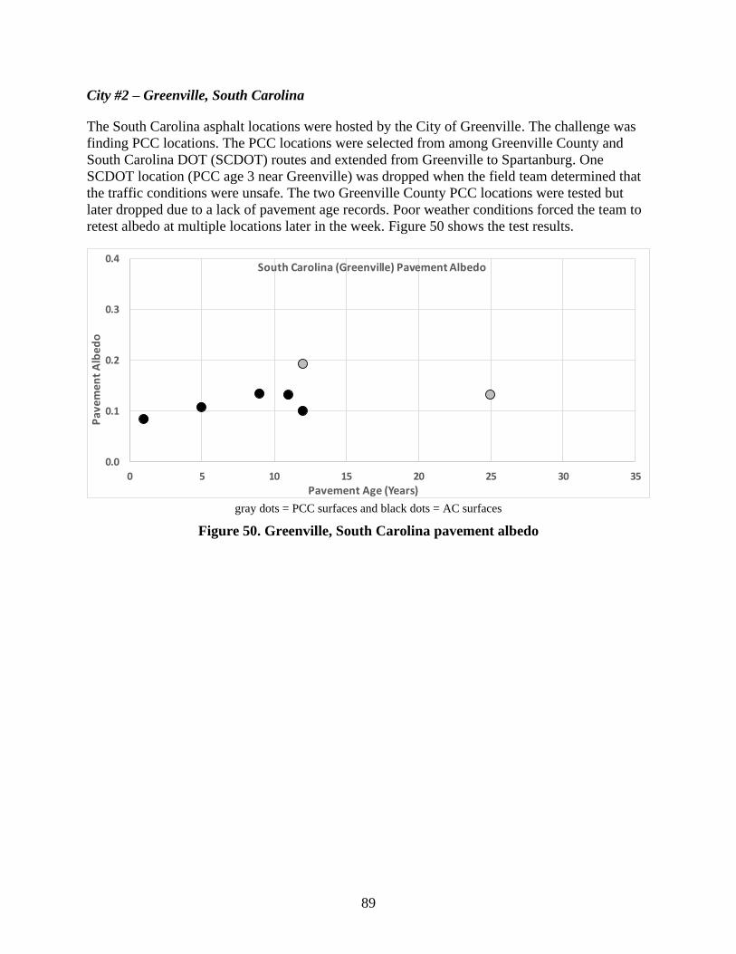
89

City #2 – Greenville, South Carolina

The South Carolina asphalt locations were hosted by the City of Greenville. The challenge was

finding PCC locations. The PCC locations were selected from among Greenville County and

South Carolina DOT (SCDOT) routes and extended from Greenville to Spartanburg. One

SCDOT location (PCC age 3 near Greenville) was dropped when the field team determined that

the traffic conditions were unsafe. The two Greenville County PCC locations were tested but

later dropped due to a lack of pavement age records. Poor weather conditions forced the team to

retest albedo at multiple locations later in the week. Figure 50 shows the test results.


Figure 50. Greenville, South Carolina pavement albedo

0.0

0.1

0.2

0.3

0.4

0 5 10 15 20 25 30 35

Pav

em

ent

Alb

ed

o


South Carolina (Greenville) Pavement Albedo

90

City #3 – Austin, Texas

The City of Austin hosted both the AC and PCC locations. All testing was completed as planned.

The sky was partly cloudy for most of the testing. Figure 51 shows the test results.


Figure 51. Austin, Texas pavement albedo

0.0

0.1

0.2

0.3

0.4

0 5 10 15 20 25 30 35

Pav

em

ent

Alb

ed

o


Texas (Austin) Pavement Albedo

91

City #4 – Mississippi (Statewide)

The Mississippi DOT hosted the AC and PCC testing and locations, which were spread from I-

20 north to Memphis, approximately the northern half of the state. The test plan was not

completed at several sites. The testing time at the 10-hour PCC site was shortened to 2 hours

because the base/subgrade temperature probe was not able to penetrate the foundation material.

Only one core was obtained at most locations because the aggregate was very hard and there was

a concern that the drill bits would not last through 10 locations. Predicted severe weather

cancelled the first scheduled trip. The skies were cloudy or partly cloudy for all locations. Figure

52 shows the test results.


Figure 52. Mississippi statewide pavement albedo

92

City #5 – South Bend, Indiana

The South Bend, Indiana, site testing results are given in Figure 53.


Figure 53. South Bend, Indiana pavement albedo

0.0

0.1

0.2

0.3

0.4

0 5 10 15 20 25 30 35

Pav

em

ent

Alb

ed

o


Indiana (South Bend) Pavement Albedo

93

City #6 – Sioux Falls, South Dakota

During the initial testing campaign at Sioux Falls, South Dakota, 10 pavements were evaluated,

including 5 concrete and 5 asphalt. However, at three of the AC locations (the three oldest

samples, with ages of 8, 13, and 23 years) it was discovered that the pavement had received a

surface chip seal-type treatment at some point following its original installation. This

circumstance likely accounts for their lower than expected albedo values, which are all lower

than those of either of the two younger samples. Therefore, these three data points were not

included in this project’s subsequent data analysis and albedo model development efforts. These

three data values are circled in red in Figure 54.

gray dots = PCC surfaces, black dots = AC surfaces, and red circles around black dots = had received

surface chip-seal-type treatment at some point following original installation

Figure 54. Sioux Falls, South Dakota pavement albedo

0.0

0.1

0.2

0.3

0.4

0 5 10 15 20 25 30 35

Pav

em

ent

Alb

ed

o


South Dakota (Sioux Falls) Pavement Albedo

94

City #7 – Iowa, Waterloo

The Waterloo, Iowa, site testing results exhibited the highest concrete albedo values of any of the

seven city testing locations, with three out of five PCC pavements showing values above 0.3

(including one with a 12-year age), and one value that was only slightly below 0.3. Figure 55

shows the test results.


Figure 55. Waterloo, Iowa pavement albedo

0.0

0.1

0.2

0.3

0.4

0 5 10 15 20 25 30 35

Pav

em

ent

Alb

ed

o


Iowa (Waterloo) Pavement Albedo

95

Comprehensive City-Level AC Pavement Albedo Results

Figure 56 provides a summary of the comprehensive set of AC pavement albedo results for this

project. The data points are either solid (i.e., northern city data) or hatched (i.e., southern city

data) to indicate their geographic locations.

solid squares = northern city and hatched squares = southern city

Figure 56. Comprehensive AC pavement albedo results

These results suggest a tendency for higher albedo values to develop within the more northerly

data grouping.

A second visual summary was also developed with these same AC pavement albedo results, in

which AC pavement albedo data recorded by Pomerantz et al. (2005) at San Jose, California,

have been added to this project’s data set. Figure 57 shows this resultant set of combined data

points, where data points from Pomerantz et al. (2005) are included as slightly smaller squares.

96

solid squares = northern city, hatched squares = southern city, and smaller dark gray squares = Pomerantz

et al. 2005 data

Figure 57. Comprehensive AC pavement albedo results plus data from Pomerantz study

These data collectively show a resultant consistency in the pattern regarding AC albedo aging.

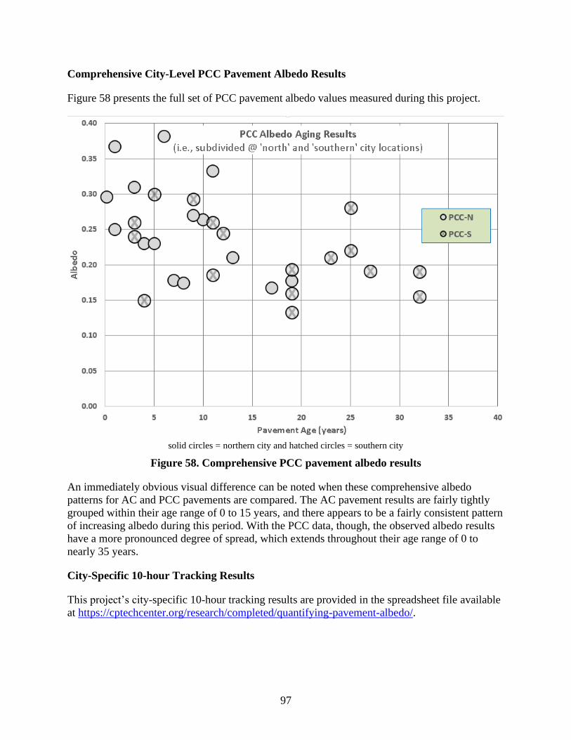
97

Comprehensive City-Level PCC Pavement Albedo Results

Figure 58 presents the full set of PCC pavement albedo values measured during this project.

solid circles = northern city and hatched circles = southern city

Figure 58. Comprehensive PCC pavement albedo results

An immediately obvious visual difference can be noted when these comprehensive albedo

patterns for AC and PCC pavements are compared. The AC pavement results are fairly tightly

grouped within their age range of 0 to 15 years, and there appears to be a fairly consistent pattern

of increasing albedo during this period. With the PCC data, though, the observed albedo results

have a more pronounced degree of spread, which extends throughout their age range of 0 to

nearly 35 years.

City-Specific 10-hour Tracking Results

This project’s city-specific 10-hour tracking results are provided in the spreadsheet file available

at https://cptechcenter.org/research/completed/quantifying-pavement-albedo/.


98

Test Track Pavement Albedo Results

This project’s test track data are provided in the spreadsheet file available at

https://cptechcenter.org/research/completed/quantifying-pavement-albedo/.

PAVEMENT CORE PROPERTIES FINDINGS

City Testing Results


This following thermal conductivity results were measured with the city-level core samples.

Figure 59 presents the PCC thermal conductivity observations (in W/(m•°C)). The left-most set

of four results (i.e., for IA-WAT, IN, MO-ISU, and SD) were obtained by the National CP Tech

Center’s laboratory, and the right-most set of four results (i.e., MO-NCAT, MS, SC, and TX)

were obtained by NCAT’s laboratory.

Figure 59. PCC thermal conductivity testing results

The CP Tech PCC thermal conductivity results ranged from ~0.65 to ~1.5 W/(m•°C), while the

NCAT results ranged from ~1 to ~1.6 W/(m•°C).

Figure 60 presents an additional correlation between these PCC thermal conductivity

observations and the thermal conductivity values cited in the literature, which were reviewed in

Chapter 3.

0

0.5

1

1.5

2

IA-W

AT

IA-W

AT

IA-W

AT

IA-W

AT

IA-W

AT

IA-W

AT IN IN IN IN

MO

-ISU

MO

-ISU

MO

-ISU

MO

-ISU

MO

-ISU SD SD SD SD SD SD

MO

-NC

AT

MO

-NC

AT

MO

-NC

AT

MO

-NC

AT

MS

MS

MS

SC SC SC SC TX

TX

TX

TX

TX

The

rmal

Co

nd

uct

ivit

y (W

/m-

oC)

City Test Site Locations

PCC-Thermal Conductivity


99

Figure 60. PCC thermal conductivity results compared to published values

Location #1 shows the literature PCC values, while locations #2 through #9 correspond with this

project’s PCC testing sites. Locations #2 through #5 correspond to CP Tech PCC core testing

results, while Locations #6 through #9 correspond to NCAT PCC core testing results.

Based on the average (i.e., red line at 1.39) and plus/minus-one-sigma (i.e., dashed red lines at

2.01 and 0.77, respectively) values for the reported literature values, it can be seen that the values

measured for this project tended to be lower than the average, and in many instances near or even

slightly below the lower minus-one-sigma boundary. However, the project values are fairly

comparable to the EICM-recommended value of 0.99 W/(m•°C).

Figure 61 presents the AC thermal conductivity observations for the same set of test locations.

Figure 61. AC thermal conductivity testing results

In this case, the CP Tech AC thermal conductivity results ranged from ~0.8 to ~1.2 W/(m•°C),

while the NCAT results ranged from ~1.1 to ~1.7 W/(m•°C).

Figure 62 examines the same sort of correlation between the AC thermal conductivity

observations and the thermal conductivity values cited in the literature, which were reviewed in

Chapter 3.

Average

Average + 1

Average - 1 0.6

0.7

0.8

0.9

1

1.1

1 2 3 4 5 6 7 8 9

kJ/k

g·oC

City Test Sites

PCC-Specific Heat

City Test Sites

0

0.5

1

1.5

2

IA-W

AT

IA-W

AT

IA-W

AT

IA-W

AT IN IN IN IN IN IN

MO

-ISU

MO

-ISU

MO

-ISU

MO

-ISU

MO


MO

-NC

AT

MO

-NC

AT

MO

-NC

AT

MO

-NC

AT

MS

MS

MS

MS

MS

SC SC SC SC SC TX

TX

TX

TX

TXTh

erm

al C

on

du

ctiv

ity

(W/m

-oC)


AC-Thermal Conductivity

100

Figure 62. AC thermal conductivity results compared to published values

Location #10 shows the literature values, while locations #11 through #18 correspond to the PCC

sites listed in the key provided in this figure. Locations #11 through #14 correspond to CP Tech

core testing results, while locations #15 through #18 correspond to NCAT core results. Here

again, based on the average (i.e., red line at 1.38) and plus/minus-one-sigma (i.e., dashed red

lines at 2.07 and 0.7, respectively) values for the reported AC literature values, it can be seen that

the values measured for this project were lower, with most values falling within the average and

minus-one-sigma range. NCAT’s Mississippi AC samples, however, were all somewhat higher,

between the average and plus-one-sigma.

Collectively, both sets of these PCC and AC thermal conductivity results are noteworthy given

that almost all of these values were consistently lower than most of the values reported in the

literature for concrete and asphalt materials (see Chapter 3). Then again, this project’s AC

thermal conductivity values are fairly comparable to the EICM-recommended value of 1.16

W/(m•°C). There was also a tendency for the CP Tech thermal conductivities to be somewhat

lower than those values observed during the NCAT tests, which might reflect either analytical

variations or actual site-related changes.

0.5

1

1.5

2

2.5

3

10 11 12 13 14 15 16 17 18 19

W/m

2-o

C

City Test Sites

AC-Thermal Conductivity

Average

Average + 1

Average - 1

0.6

0.7

0.8

0.9

1

1.1

10 11 12 13 14 15 16 17 18

kJ/k

g·oC

City Test Sites

AC-Specific Heat

City Test Sites

101

Specific Heat

The following specific heat results were also measured for the city-level core samples. Figure 63

presents the PCC specific heat observations (in kJ/(kg•°C)).

Figure 63. PCC specific heat testing results

The left-most set of four results (i.e., for IA-WAT, IN, MO-ISU, and SD) were obtained by the

National CP Tech Center’s laboratory, and the right-most set of four results (i.e., MO-NCAT,

MS, SC, and TX) were obtained by NCAT’s laboratory. The CP Tech PCC specific heat results

ranged from ~0.55 to ~0.97 kJ/(kg•°C), while the NCAT results ranged from ~0.85 to ~0.9

kJ/(kg•°C).

Figure 64 provides the correlation between these PCC specific heat observations and the specific

heat values cited in the literature, which were reviewed in Chapter 3.

Figure 64. PCC specific heat results compared to published values

Locations #2 through #5 represent the CP Tech core samples, and locations #6 through #9

represent the NCAT core samples. Based on the average (i.e., red line at 0.92 kJ/(kg•°C)) and

plus/minus-one-sigma (i.e., dashed red lines at 1.09 and 0.74 kJ/(kg•°C), respectively) values for

these reported literature values, it can be seen that the values measured for this project tended to

be lower than the published average, and in some instances near or even slightly below the

published minus-one-sigma boundary. Compared to the EICM-recommended value, however,

00.10.20.30.40.50.60.70.80.9

1

IA-W

AT

IA-W

AT

IA-W

AT

IA-W

AT

IA-W

AT

IA-W

AT IN IN IN IN

MO

-ISU

MO

-ISU

MO

-ISU

MO

-ISU

MO


MO

-NC

AT

MO

-NC

AT

MO

-NC

AT

MO

-NC

AT

MS

MS

MS

SC SC SC SC TX

TX

TX

TX

TXSp

eci

fic

He

t (k

J/kg

-oC


PCC-Specific Heat

0.6

0.7

0.8

0.9

1

1.1

1 2 3 4 5 6 7 8 9

kJ/k

g·oC

City Test Sites

PCC-Specific Heat

Average

Average + 1

Average - 1

City Test Sites

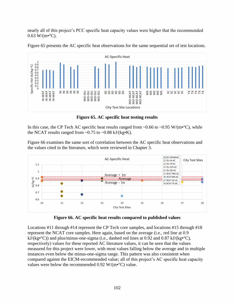
102

nearly all of this project’s PCC specific heat capacity values were higher that the recommended

0.63 W/(m•°C).

Figure 65 presents the AC specific heat observations for the same sequential set of test locations.

Figure 65. AC specific heat testing results

In this case, the CP Tech AC specific heat results ranged from ~0.66 to ~0.95 W/(m•°C), while

the NCAT results ranged from ~0.75 to ~0.88 kJ/(kg•K).

Figure 66 examines the same sort of correlation between the AC specific heat observations and

the values cited in the literature, which were reviewed in Chapter 3.

Figure 66. AC specific heat results compared to published values


represent the NCAT core samples. Here again, based on the average (i.e., red line at 0.9

kJ/(kg•°C)) and plus/minus-one-sigma (i.e., dashed red lines at 0.92 and 0.87 kJ/(kg•°C),

respectively) values for these reported AC literature values, it can be seen that the values

measured for this project were lower, with most values falling below the average and in multiple

instances even below the minus-one-sigma range. This pattern was also consistent when

compared against the EICM-recommended value; all of this project’s AC specific heat capacity

values were below the recommended 0.92 W/(m•°C) value.

00.10.20.30.40.50.60.70.80.9

1

IA-W

AT

IA-W

AT

IA-W

AT

IA-W


MO

-ISU

MO

-ISU

MO

-ISU

MO

-ISU

MO


MO

-NC

AT

MO

-NC

AT

MO

-NC

AT

MO

-NC

AT

MS

MS

MS

MS

MS

SC SC SC SC SC TX

TX

TX

TX

TXSp

eci

fic

He

t (k

J/kg

-oC

)


AC-Specific Heat

0.6

0.7

0.8

0.9

1

1.1

10 11 12 13 14 15 16 17 18

kJ/k

g·oC

City Test Sites

AC-Specific Heat

Average + 1

Average - 1Average

City Test Sites

103

As with the thermal conductivity results, both sets of these PCC and AC measurements are

noteworthy given that almost all of these values were consistently lower than values reported in

the literature for concrete and asphalt materials. Once again, there was a nominal tendency for

the National CP Tech Center’s specific heat values to be somewhat lower than the values

observed during the NCAT tests, which might reflect either analytical variations or actual site-

related changes. However, this project’s results suggest that future estimates of pavement

specific heat values should be reduced in light of current published values.

Emissivity

The following emissivity results were also measured with the city-level core samples. Figure 67

presents the PCC emissivity observations with dimensionless units.

Figure 67. PCC emissivity testing results

The left-most set of four PCC emissivity results, from the National CP Tech Center, ranged from

~0.88 to ~0.96, while the right-most set of four results, from NCAT, ranged from ~0.88 to ~0.92.

Figure 68 provides the correlation between these PCC emissivity observations and the emissivity

values cited in the literature, which were reviewed in Chapter 3.

Figure 68. PCC emissivity results compared to published values


represent the NCAT core samples. Based on the average (i.e., red line at 0.94) and plus/minus-

one-sigma (i.e., dashed red lines at ~0.97 and ~0.91, respectively) values for these reported

0.8

0.85

0.9

0.95

1

IA-W

AT

IA-W

AT

IA-W

AT

IA-W

AT

IA-W

AT

IA-W

AT IN IN IN IN

MO

-ISU

MO

-ISU

MO

-ISU

MO

-ISU

MO


MO

-NC

AT

MO

-NC

AT

MO

-NC

AT

MO

-NC

AT

MS

MS

MS

SC SC SC SC TX

TX

TX

TX

TX

Emis

sivi

ty


PCC-Emissivity

0.8

0.82

0.84

0.86

0.88

0.9

0.92

0.94

0.96

0.98

1

1 2 3 4 5 6 7 8 9

Emis

sivi

ty (

dim

en

sio

nle

ss)

City Test Sites

PCC-Emissivity

Average

Average + 1

Average - 1

City Test Sites

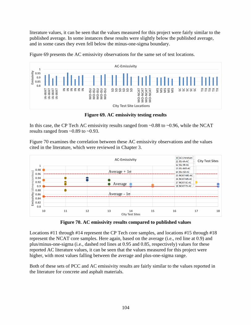
104

literature values, it can be seen that the values measured for this project were fairly similar to the

published average. In some instances these results were slightly below the published average,

and in some cases they even fell below the minus-one-sigma boundary.

Figure 69 presents the AC emissivity observations for the same set of test locations.

Figure 69. AC emissivity testing results

In this case, the CP Tech AC emissivity results ranged from ~0.88 to ~0.96, while the NCAT

results ranged from ~0.89 to ~0.93.

Figure 70 examines the correlation between these AC emissivity observations and the values

cited in the literature, which were reviewed in Chapter 3.

Figure 70. AC emissivity results compared to published values


represent the NCAT core samples. Here again, based on the average (i.e., red line at 0.9) and

plus/minus-one-sigma (i.e., dashed red lines at 0.95 and 0.85, respectively) values for these

reported AC literature values, it can be seen that the values measured for this project were

higher, with most values falling between the average and plus-one-sigma range.

Both of these sets of PCC and AC emissivity results are fairly similar to the values reported in

the literature for concrete and asphalt materials.

0.8

0.85

0.9

0.95

1

IA-W

AT

IA-W

AT

IA-W

AT

IA-W


MO

-ISU

MO

-ISU

MO

-ISU

MO

-ISU

MO


MO

-NC

AT

MO

-NC

AT

MO

-NC

AT

MO

-NC

AT

MS

MS

MS

MS

MS

SC SC SC SC SC TX

TX

TX

TX

TX

Emis

sivi

ty


AC-Emissivity

0.8

0.82

0.84

0.86

0.88

0.9

0.92

0.94

0.96

0.98

1

10 11 12 13 14 15 16 17 18

Emis

sivi

ty (

dim

en

sio

nle

ss)

City Test Sites

AC-Emissivity

Average

Average + 1

Average - 1

City Test Sites

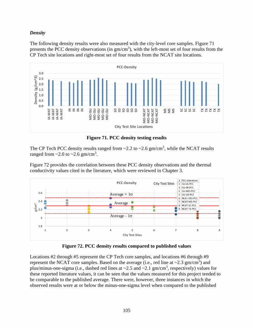
105

Density

The following density results were also measured with the city-level core samples. Figure 71

presents the PCC density observations (in gm/cm3), with the left-most set of four results from the

CP Tech site locations and right-most set of four results from the NCAT site locations.

Figure 71. PCC density testing results

The CP Tech PCC density results ranged from ~2.2 to ~2.6 gm/cm3, while the NCAT results

ranged from ~2.0 to ~2.6 gm/cm3.

Figure 72 provides the correlation between these PCC density observations and the thermal

conductivity values cited in the literature, which were reviewed in Chapter 3.

Figure 72. PCC density results compared to published values


represent the NCAT core samples. Based on the average (i.e., red line at ~2.3 gm/cm3) and

plus/minus-one-sigma (i.e., dashed red lines at ~2.5 and ~2.1 gm/cm3, respectively) values for

these reported literature values, it can be seen that the values measured for this project tended to

be comparable to the published average. There were, however, three instances in which the

observed results were at or below the minus-one-sigma level when compared to the published

0.0

0.5

1.0

1.5

2.0

2.5

3.0

IA-W

AT

IA-W

AT

IA-W

AT

IA-W

AT IN IN IN IN

MO

-ISU

MO

-ISU

MO

-ISU

MO

-ISU

MO


MO

-NC

AT

MO

-NC

AT

MO

-NC

AT

MO

-NC

AT

MS

MS

MS

SC SC SC SC TX TX TX TX TX

De

nsi

ty (

g/c

m^3

)


PCC-Density

1.8

2

2.2

2.4

2.6

1 2 3 4 5 6 7 8 9

g/cm

3

City Test Sites

PCC-Density

Average

Average + 1

Average - 1

City Test Sites

106

literature: at the National CP Tech Center’s Iowa location and NCAT’s South Carolina and

Texas locations.

Figure 73 presents the AC density observations for the same sequential set of test locations.

Figure 73. AC density testing results

In this case, the CP Tech AC density results ranged from ~2.2 to ~2.5 gm/cm3, while the NCAT

results ranged from ~2.1 to ~2.3 gm/cm3.

Figure 74 examines the same sort of correlation between these AC density observations and the

values cited in the literature, which were reviewed for AC materials in Chapter 3.

Figure 74. AC density results compared to published values


represent the NCAT core samples. Based on the average (i.e., red line at 2.2 gm/cm3) and

plus/minus-one-sigma (i.e., dashed red lines at 2.4 and 2.0 gm/cm3, respectively) values for these

reported AC literature values, it can be seen that the pavement density measurements for this

project tended to be somewhat higher, with most values falling above the average, and in two

instances (i.e., the CP Tech and NCAT Missouri locations) even exceeding the plus-one-sigma

range.

0.0

0.5

1.0

1.5

2.0

2.5

3.0

IA-W

AT

IA-W

AT

IA-W


MO

-ISU

MO

-ISU

MO

-ISU

MO

-ISU

MO


MO

-NC

AT

MO

-NC

AT

MO

-NC

AT

MO

-NC

AT

MS

MS

MS

MS

MS

SC SC SC SC SC TX TX TX TX TX

De

nsi

ty (

g/c

m^3

)


AC-Density

Average

Average + 1

Average - 1

City Test Sites

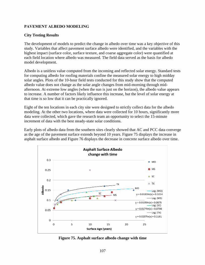
107

PAVEMENT ALBEDO MODELING

City Testing Results

The development of models to predict the change in albedo over time was a key objective of this

study. Variables that affect pavement surface albedo were identified, and the variables with the

highest impact (surface color, surface texture, and coarse aggregate color) were quantified at

each field location where albedo was measured. The field data served as the basis for albedo

model development.

Albedo is a unitless value computed from the incoming and reflected solar energy. Standard tests

for computing albedo for roofing materials confine the measured solar energy to high midday

solar angles. Plots of the 10-hour field tests conducted for this study show that the computed

albedo value does not change as the solar angle changes from mid-morning through mid-

afternoon. At extreme low angles (when the sun is just on the horizon), the albedo value appears

to increase. A number of factors likely influence this increase, but the level of solar energy at

that time is so low that it can be practically ignored.

Eight of the ten locations in each city site were designed to strictly collect data for the albedo

modeling. At the other two locations, where data were collected for 10 hours, significantly more

data were collected, which gave the research team an opportunity to select the 15-minute

increment of data with the best steady-state solar conditions.

Early plots of albedo data from the southern sites clearly showed that AC and PCC data converge

as the age of the pavement surface extends beyond 10 years. Figure 75 displays the increase in

asphalt surface albedo and Figure 76 displays the decrease in concrete surface albedo over time.

Figure 75. Asphalt surface albedo change with time

108

Figure 76. Concrete surface albedo change with time

Separate data sets for AC and PCC were used to account for the differences in the early-life

progression of the albedo values.

The primary data used in the development of the albedo models are as follows:

• Pavement surface age.

• Color of the pavement surface (wheel path and centerline).

• Texture of the pavement surface (wheel path and centerline).

• Color of the predominant coarse aggregate in the surface AC/PCC mixture.

Pavement surface color and surface texture data were collected at both the centerline and in the

wheel paths because the albedometer measures energy over a 3.7 m diameter when placed at the

prescribed height of 0.5 m from the surface. This measured area includes both wheel path surface

and centerline surface.

Preliminary analysis of the surface color data showed that there was no consistent, practical

difference between the centerline and wheel path (see Figures 77 through 79). This finding

allowed development of the albedo model to continue without concern for bias from the color of

the area measured.

109

Figure 77. Asphalt surface centerline and wheel path color

Figure 78. Concrete surface centerline and wheel path color

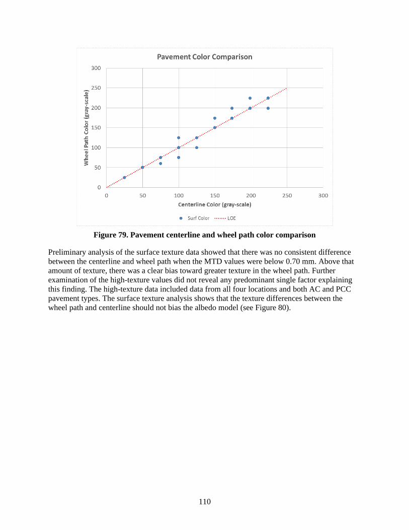
110

Figure 79. Pavement centerline and wheel path color comparison

Preliminary analysis of the surface texture data showed that there was no consistent difference

between the centerline and wheel path when the MTD values were below 0.70 mm. Above that

amount of texture, there was a clear bias toward greater texture in the wheel path. Further

examination of the high-texture values did not reveal any predominant single factor explaining

this finding. The high-texture data included data from all four locations and both AC and PCC

pavement types. The surface texture analysis shows that the texture differences between the

wheel path and centerline should not bias the albedo model (see Figure 80).

111

Figure 80. Pavement centerline and wheel path surface texture comparison

The laboratory testing included controlled digital imaging of the core surface and cut face to

determine the surface color and predominant coarse aggregate color. The images were converted

to grayscale for a direct comparison to the grayscale chart. It was assumed that controlled

laboratory grayscale imaging would result in more consistent values for the albedo analysis. The

comparison of AC surfaces between the field-measured centerline surface color and the

laboratory core surface color (cores were taken from the centerline) resulted in two findings.

One, the laboratory-measured colors on most of the AC cores showed a narrower range of

laboratory colors, between 25 and 55, compared to the field-measured colors, which ranged from

25 to 174. Two, the dominant AC coarse aggregate color was consistent between cores taken

from the same location. The comparison of the PCC surfaces showed a predominant grouping,

with the laboratory-measured surface color ranging from 25 to 87 and the field-measured surface

color ranging from 150 to 224. The dominant PCC coarse aggregate color was consistent for

three locations but split for the Texas location. The laboratory color analysis established that

coarse aggregate color was consistent for most sites, and the laboratory-measured core surface

color displayed a darker, narrower grayscale color compared to the field-measured color (Figures

81 through 84).

112

Figure 81. Asphalt field surface color and laboratory surface color comparison

Figure 82. Asphalt field surface color and laboratory aggregate color comparison

113

Figure 83. Concrete field surface color and laboratory surface color comparison

Figure 84. Concrete field surface color and laboratory aggregate color comparison

Initial attempts to develop the model used statistical approaches to determine a general

regression model. The first step was to apply a best subsets regression tool to determine the

114

combination of variables that would account for a majority of the albedo change. The second

step was to analyze the variables within the selected regression.

The best subset of variables for the AC model included age, field centerline color, field wheel

path color, wheel path texture, and a combination of age and laboratory core surface color. The

regression analysis using these variables showed that the combined age/surface color accounted

for 65% of the model. Pavement surface age and field surface centerline color equally accounted

for 16% each. These three variables accounted for 97% of the AC model. Field wheel path color

and surface texture had very little effect on the albedo value. The AC model had an adjusted R2

of 97% (see Figure 85).

Analysis Variables Legend

x1=Age = pavement surface age (years)

x2=CTL CLR = pavement centerline field surface color (grayscale value)

x3=WP CLR = pavement wheel path field surface color (grayscale value)

x4=SURF CLR = pavement centerline core laboratory measured color (grayscale value)

x5=AGGR CLR = asphalt surface mixture coarse aggregate color (grayscale value)

x6=CTL MTD = mean texture depth of the pavement surface near centerline of the test lane

(mm)

x7=WP MTD = mean texture depth of the pavement surface near wheel path (mm)

AC Pvmt Best Subsets Regression: ALBEDO versus x1, x2, ... Response is ALBEDO

x x

Mallows x x x x x x x 1 1

Vars R-Sq R-Sq(adj) Cp S 1 2 3 4 5 6 7 1 4

1 76.9 75.3 87.1 0.019368 X

1 46.6 42.7 217.7 0.029486 X

2 91.0 89.6 28.8 0.012580 X X

2 89.7 88.1 34.4 0.013446 X X

3 96.4 95.4 7.7 0.0083125 X X X

3 93.9 92.3 18.3 0.010785 X X X

4 97.2 96.1 6.2 0.0076729 X X X X

4 96.6 95.3 8.8 0.0084287 X X X X

5 98.3 97.4 3.5 0.0062951 X X X X X

5 98.0 96.9 4.8 0.0068108 X X X X X

6 98.6 97.7 4.0 0.0059583 X X X X X X

6 98.3 97.2 5.2 0.0065275 X X X X X X

7 98.6 97.4 6.0 0.0063057 X X X X X X X

7 98.6 97.4 6.0 0.0063179 X X X X X X X

8 98.6 97.0 8.0 0.0067396 X X X X X X X X

8 98.6 97.0 8.0 0.0067411 X X X X X X X X

9 98.6 96.5 10.0 0.0072788 X X X X X X X X X

General Regression Analysis: ALBEDO versus x1, x2, x3, x7, x14 Regression Equation

ALBEDO = 0.0526124 - 0.00634018 x1 + 0.000714018 x2 - 0.000480425 x3 + 0.035456 x7 +

0.000222033 x14

Coefficients

115

Term Coef SE Coef T P

Constant 0.0526124 0.0074098 7.1004 0.000

x1 -0.0063402 0.0007971 -7.9540 0.000

x2 0.0007140 0.0001307 5.4614 0.000

x3 -0.0004804 0.0001471 -3.2652 0.008

x7 0.0354560 0.0097473 3.6375 0.005

x14 0.0002220 0.0000115 19.3781 0.000

Summary of Model

S = 0.00629506 R-Sq = 98.26% R-Sq(adj) = 97.39%

PRESS = 0.00126012 R-Sq(pred) = 94.47%

Analysis of Variance

Source DF Seq SS Adj SS Adj MS F P

Regression 5 0.0223787 0.0223787 0.0044757 112.945 0.0000000

x1 1 0.0035682 0.0025071 0.0025071 63.266 0.0000124

x2 1 0.0039077 0.0011820 0.0011820 29.827 0.0002764

x3 1 0.0000005 0.0004225 0.0004225 10.662 0.0084985

x7 1 0.0000217 0.0005243 0.0005243 13.232 0.0045554

x14 1 0.0148807 0.0148807 0.0148807 375.511 0.0000000

Error 10 0.0003963 0.0003963 0.0000396

Total 15 0.0227750

Fits and Diagnostics for Unusual Observations

Obs ALBEDO Fit SE Fit Residual St Resid

2 0.14 0.151069 0.0038489 -0.0110691 -2.22213 R

R denotes an observation with a large standardized residual.

Figure 85. Printout. Regression analysis of asphalt albedo variables

For the PCC model, the best subset of variables included age (as single, squared, and cubed

terms), centerline texture, and a combination of field centerline color and centerline texture. The

regression analysis using these variables revealed that the combination of color and texture

accounted for 61% of the model. The centerline texture and cubed age variables accounted for

14% each. These three variables accounted for 89% of the PCC model. The unexplained residual

error was 8%. Age and squared age had very little effect on the albedo value. The PCC model

had an adjusted R2 of 85% (see Figure 86).

Analysis Variables Legend

x1=Age = pavement surface age (years)

x2=CTL CLR = pavement centerline field surface color (grayscale value)

x3=WP CLR = pavement wheel path field surface color (grayscale value)

x4=SURF CLR = pavement centerline core laboratory measured color (grayscale value)

x5=Aggr CLR = concrete surface mixture coarse aggregate color (grayscale value)

x6=CTL MTD = mean texture depth of the pavement surface near centerline of the test lane

(mm)

x7=WP MTD = mean texture depth of the pavement surface near wheel path (mm)

116

Best Subsets Regression: ALBEDO versus x1, x2, ... Response is ALBEDO

x

1

x x

x 1 1

Mallows x x x x x x x 2 x x

Vars R-Sq R-Sq(adj) Cp S 1 2 3 4 5 6 7 6 1 1

1 48.4 43.7 22.3 0.034836 X

1 47.7 42.9 22.7 0.035087 X

2 62.2 54.7 15.9 0.031260 X X

2 55.8 47.0 19.8 0.033809 X X

3 75.3 67.1 10.0 0.026646 X X X

3 72.0 62.7 12.0 0.028376 X X X

4 83.5 75.2 7.0 0.023136 X X X X

4 80.8 71.2 8.7 0.024935 X X X X

5 91.6 85.7 4.1 0.017591 X X X X X

5 87.3 78.3 6.7 0.021629 X X X X X

6 94.6 89.1 4.3 0.015324 X X X X X X

6 92.3 84.6 5.7 0.018251 X X X X X X

7 96.0 90.5 5.4 0.014315 X X X X X X X

7 94.9 87.7 6.1 0.016298 X X X X X X X

8 96.2 88.5 7.3 0.015768 X X X X X X X X

8 96.0 88.1 7.4 0.015998 X X X X X X X X

9 96.3 85.0 9.3 0.017967 X X X X X X X X X

9 96.2 84.8 9.3 0.018121 X X X X X X X X X

10 96.7 80.2 11.0 0.020661 X X X X X X X X X X

General Regression Analysis: ALBEDO versus x1, x6, x26, x1x1, x1x1x1 Regression Equation

ALBEDO = 0.178761 + 0.0155878 x1 - 0.438614 x6 + 0.00260781 x26 - 0.00138723

x1x1 + 2.86051e-005 x1x1x1

Coefficients

Term Coef SE Coef T P

Constant 0.178761 0.0216739 8.24774 0.000

x1 0.015588 0.0059610 2.61498 0.035

x6 -0.438614 0.0662679 -6.61880 0.000

x26 0.002608 0.0003260 7.99841 0.000

x1x1 -0.001387 0.0004126 -3.36228 0.012

x1x1x1 0.000029 0.0000080 3.55897 0.009

Summary of Model

S = 0.0175909 R-Sq = 91.63% R-Sq(adj) = 85.65%

PRESS = 0.00982921 R-Sq(pred) = 62.02%

Analysis of Variance

Source DF Seq SS Adj SS Adj MS F P

Regression 5 0.0237109 0.0237109 0.0047422 15.3251 0.0011905

x1 1 0.0001676 0.0021160 0.0021160 6.8381 0.0346615

x6 1 0.0033570 0.0135560 0.0135560 43.8085 0.0002990

x26 1 0.0159623 0.0197962 0.0197962 63.9745 0.0000913

x1x1 1 0.0003045 0.0034982 0.0034982 11.3049 0.0120467

x1x1x1 1 0.0039194 0.0039194 0.0039194 12.6663 0.0092321

Error 7 0.0021661 0.0021661 0.0003094

Total 12 0.0258769

Fits and Diagnostics for Unusual Observations

No unusual observations

Figure 86. Printout. Regression analysis of concrete albedo variables

117

When the measured surface parameters from a specific test location were entered into either

regression model, the predicted albedo did not demonstrate a good match, particularly for

generating an albedo trend over time. One possible explanation for the poor fit is that the

regression model was based on using all AC measurements from all locations to determine the

best fit; a similar approach was used for the PCC data. In Figures 75 and 76 it can be observed

that each location demonstrated an independent albedo change with time. The unique albedo

trend for each location may have diminished the strength of a combined data set for each

pavement type.

Asphalt Surface Albedo Model

The next approach in developing the model was to consider the observation that each test

location generated a unique albedo performance curve. The approach to developing a model for

AC pavement albedo was to start with the logarithmic trend equation for albedo versus time for

each location. The general equation for each trend line used the form shown in Figure 87.

y=a×ln(x)+b

Figure 87. General form of asphalt albedo model

Where:

y = the albedo value (proportion of reflected solar energy).

a = an equation constant.

x = the pavement surface age (years).

b = an equation constant.

It should be noted that this modeled y variable also equals the albedo value, R, previously cited

in Figure 26. This modeled y value is derived using Excel’s data regression analysis routine.

As seen in Figure 88, one of the eight trends did not conform to the group. The data for Sioux

Falls, South Dakota were examined and dropped from further analysis.

118

Figure 88. Field-measured asphalt surface albedo change with time

The equation constants are listed in Table 23 in order from highest albedo trend to lowest albedo

trend.

Table 23. Asphalt albedo trend equation constants and aggregate color by field location

Albedo Location y (albedo) = a ln(age) + b

Aggr

CLR

higher ISU 0.0338 0.1275

IA 0.0382 0.1011 204 IN 0.0276 0.1083 208 TX 0.0207 0.1161 145 MO 0.0183 0.1014 107 SC 0.0174 0.0798 88

lower MS 0.0135 0.0875 58 SD* -0.009 0.1622

*Data set removed from further consideration

The “a” constant for each equation similarly follows from a higher value to lower value. The “b”

constant generally follows the same high-to-low trend, but individual values are mixed.

The next step in the development of the AC albedo model was to select the best pavement

variable to incorporate into the “a” and “b” constants. The pavement surface colors demonstrated

a strong correlation to the change in albedo, as identified in the previous regression analysis

(Figures 85) for variables X2 and X4. These values change with time, so they were not

considered a good variable to distinguish between locations. It was noted that coarse aggregate

119

color followed the same high-to-low pattern as the albedo-to-age trends. The analysis of

aggregate color displayed in Figure 82 shows that aggregate color is a reasonable constant for

each location.

The average aggregate color for each location was added to Table 23. At this point in the

model’s development, only the aggregate color values for four sites were used for the initial

model development. The remaining sites were to be used to validate the model. The equation

constants for each location were matched with the aggregate color values and plotted in Figure

89.

Figure 89. Relationship of asphalt albedo model constants and location coarse aggregate

color

The constants and aggregate color values demonstrated a good correlation. A linear trend line for

each equation constant versus aggregate color was determined and the equation substituted for

each constant to form the equation in Figure 90.

AC albedo=(0.00008×Aggr CLR+0.0094)×ln(AGE)+(0.0004×Aggr CLR+0.0587)

Figure 90. Asphalt albedo model using pavement age and aggregate color

Where:

AC albedo = the predicted albedo of the asphalt surface.

Aggr CLR = the color of the predominant coarse aggregate in the asphalt mix (grayscale value).

AGE = the age of the asphalt pavement surface (years).

120

The model was tested to examine its fit to actual data. The first step was to compare the trend

lines from Figure 88 to the model prediction curves generated from the equation in Figure 90.

Figure 91 displays the results of this comparison.

Figure 91. Measured field albedo trend and asphalt model albedo trend

The match is very good for three of the four locations. The predicted albedo for South Carolina is

higher than the field data trend line, but the difference is less than 0.02.

The second step in the model verification was to look at the actual field data and compare the

measured albedo for each test site against the predicted albedo from the model using the

pavement surface age and measured pavement aggregate color. A simple comparison plot of the

measured albedo against the predicted albedo is shown in Figure 92.

121

Figure 92. Measured asphalt site albedo and asphalt model albedo comparison

Considering the variation in the actual field-measured albedo values, the deviation from the line

of equality is reasonable. Two values, one positive and one negative, deviate more than 0.07 and

reflect the two extreme values in the Texas data set. Two values, both positive, deviate more than

0.03 and represent one measured site in Missouri and one in South Carolina. The comparison

was examined using a histogram, shown in Figure 93.

Figure 93. Difference between measure asphalt site albedo and asphalt model-computed

albedo

Of the 19 compared values, 12 of the albedo differences are grouped between -0.02 and 0.02.

This comparison of the field-measured albedo and model-predicted albedo confirm that the

model is reasonable.

Data from the Indiana and Iowa locations were used to validate the model. Age and aggregate

color values for each site were entered into the albedo model to compute a predicted albedo

value. The field-measured albedo data and trend line were compared to the predicted albedo

value trend line as shown in Figure 94.

122

Figure 94. Asphalt albedo model validation measured field trend and computed model

trend

The trend line for the predicted albedo values is higher than the trend line for the measured

values. A histogram of the distribution of the differences between the measured values and

predicted values is shown in Figure 95.

Figure 95. Asphalt model validation histogram of difference between field-measured albedo

and model albedo

The differences range between -0.02 and 0.06, which is a similar range to that of the differences

created by the original data, as shown in Figure 93. The basic statistics for the differences from

all six locations combined are an average difference of 0.008 with a standard deviation of 0.029.

123

With the added evidence that the model was predicting equal or higher albedo values, the model

was recalibrated with the larger data set of six locations. Two additional albedo

constants/aggregate color values were added and new linear trend lines were formed, as shown in

Figure 96.

Figure 96. Recalibration of asphalt model constants with location aggregate color

The slope and intercept constants for the new linear trend line changed with the newly added

aggregate color values above 200. Using the new “a” and “b” constants, a new asphalt albedo

model was generated, given as the equation in Figure 97.

AC albedo=(0.0001×Aggr CLR+0.0033)×ln(AGE)+(0.0001×Aggr CLR 0.0812)

Figure 97. Asphalt albedo model using pavement age and aggregate color

Where:

AC albedo = the predicted albedo of the asphalt surface.

Aggr CLR = the color of the predominant coarse aggregate in the asphalt mix (grayscale value).

AGE = the age of the asphalt pavement surface (years).

A new set of albedo curves was graphed to compare the field-measured albedo trend lines with

the recalibrated model trend lines, as shown in Figure 98.

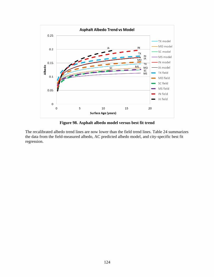
124

Figure 98. Asphalt albedo model versus best fit trend

The recalibrated albedo trend lines are now lower than the field trend lines. Table 24 summarizes

the data from the field-measured albedo, AC predicted albedo model, and city-specific best fit

regression.

125

Table 24. Asphalt variables and computed albedo values for each site S

tate

Sit

e

Age

Alb

edo

Aggr

CL

R Albedo model

Site-specific best

fit trend

Mod

el

Alb

edo

del

ta

Bes

t F

it

Tre

nd

del

ta

MO 6 1 0.1 112.5 0.092 -0.008 0.101 0.001

MO 7 4 0.15 125 0.116 -0.034 0.127 -0.023

MO 9 6 0.1 125 0.122 0.022 0.134 0.034

MO 8 22 0.15 75 0.122 -0.028 0.158 0.008

MO 10 14 0.17 100 0.126 -0.044 0.150 -0.020

MS 7 0.1 0.06 58 0.066 0.006 0.056 -0.004

MS 9 2 0.09 37.5 0.090 -0.000 0.097 0.007

MS 4 10 0.11 50 0.105 -0.005 0.119 0.009

MS 10 14 0.12 87.5 0.122 0.002 0.123 0.003

MS 1 16 0.14 58 0.112 -0.028 0.125 -0.015

SC 1 1 0.08 75 0.089 0.009 0.080 -0.000

SC 3 5 0.1 92 0.111 0.011 0.108 0.008

SC 5 12 0.11 100 0.124 0.014 0.123 0.013

SC 2 9 0.14 75 0.112 -0.028 0.118 -0.022

SC 4 11 0.12 100 0.123 0.003 0.122 0.002

TX 5 0.3 0.08 150 0.074 -0.006 0.091 0.011

TX 4 2 0.13 137.5 0.107 -0.023 0.130 0.000

TX 3 10 0.25 150 0.138 -0.112 0.164 -0.086

TX 1 17 0.1 142 0.145 0.0450 0.175 0.075

IN 2 1 0.11 188 0.100 -0.010 0.104 -0.006

IN 3 4 0.15 232 0.141 -0.009 0.149 -0.001

IN 5 14 0.21 212 0.167 -0.043 0.190 -0.020

IN 1 9 0.14 199 0.152 0.012 0.175 0.035

IA 10 10 0.188 205 0.156 -0.031 0.189 0.001

IA 9 9 0.181 204 0.154 -0.027 0.185 0.004

IA 12 12 0.2 193 0.157 -0.043 0.196 -0.004

IA 3 3 0.144 214 0.130 -0.014 0.143 -0.001 Average -0.014 Average 0.0003 Std Dev 0.029 Std Dev 0.026

Aggr CLR = the color of the predominant coarse aggregate in the asphalt surface mix (grayscale)

126

The individual data point comparisons to the line of equality are shown in Figure 99.

Figure 99. Measured asphalt site albedo and recalibrated model albedo comparison

The data points follow the line of equality up to a predicted albedo value of 0.15. Above that

value, the predicted values are lower than the measured values. The histogram of the predicted

and measured albedo differences now shifts to a range of -0.04 to 0.02, as shown in Figure 100.

Figure 100. Difference between measured asphalt site albedo and recalibrated asphalt

model computed albedo

In basic statistical terms, the average difference for the recalibrated model is -0.014 with a

standard deviation of 0.029. The average shifted down by 0.022, but the standard deviation

remained the same. The standard deviation (0.029) for the model-computed albedo compared to

the field-measured albedo is similar to the standard deviation of the difference between the

location-specific best fit regressions of the actual field-measured albedo (0.026).

127

Concrete Surface Albedo Model

The process used to develop the AC model was applied to the PCC data. The PCC albedo data

were plotted with pavement surface age. Each set of data for a location was fitted with a trend

line using the power equation shown in Figure 101.

=a×x^b

Figure 101. General form of the concrete albedo model

Where:

y = the albedo value (proportion of reflected solar energy).

a = an equation constant.

x = the pavement surface age (years).

b = an equation constant.

It should be noted that this modeled y variable also equals the albedo value, R, previously cited

in Figure 26. This modeled y value is derived using Excel’s data regression analysis routine.

The power equation function created a trend line shape comparable to the overall trend of the

PCC albedo data over time. Figure 102 displays the trend lines for the PCC surface albedo data.

Figure 102. Field-measured concrete surface albedo change with time

128

The equation constants are summarized in Table 25.

Table 25. Concrete albedo trend equation constants, texture, and aggregate color by field

location

Location

y

(albedo) = a age ^b

CTL

MTD

Aggr

CLR

Aggr CLR

/CTL MTD

IA High 0.3603 -0.059 0.54 177 327.3

ISU

0.329 -0.091

MS

0.3298 -0.16 0.71 69 96.8

MO

0.3086 -0.152 0.37 129 346.0

IN

0.2584 -0.08 0.94 173 184.6

SD

0.2238 -0.109 0.66 142 214.9

TX Low 0.2029 -0.069 0.58 103 177.8

Aggr CLR = the color of the predominant coarse aggregate in the concrete mix (grayscale)

CTL MTD = the mean texture depth of the of the pavement surface near centerline of the test lane (mm)

The locations are listed from highest measured albedo to lowest, and the “a” constant follows the

same order. The “b” constant does not follow the high-to-low trend.

The regression model analysis shows that pavement surface texture was a predominant variable.

This variable was not as consistent as aggregate color, however, because each surface is finished

with a texture specified for that site, and texture is influenced by material and construction

quality. As with the AC model development, the pavement surface color variables were not used.

The strong correlation between albedo and the pavement mixture’s predominant coarse

aggregate in the AC model was applied to the development of the PCC model. A review of the

aggregate color for each location showed that the color was reasonably uniform, with a few

exceptions. The common aggregate color for each a location is expected because both the AC

and PCC mixtures at each site were likely to have been produced using aggregate from quarries

with the same geology. Both the surface texture average and aggregate color average were added

to Table 25. Neither set of data followed the same ranking as the albedo trend lines. Due to the

variability in the surface texture and aggregate color values between locations, the decision was

made to build the model with data from all six locations. The equation constants for each

location were matched with the surface texture values and are plotted in Figure 103.

129

Figure 103. Relationship of concrete albedo model constants and location surface texture

The equation constants and surface texture values demonstrated a fair correlation with a linear

trend. The linear trend equation was substituted into the albedo trend equation. The predicted

albedo values for each site were computed and compared to the field-measured albedo values.

Table 26 shows a summary of the data resulting from the PCC model using surface texture and

pavement surface age. The average difference between these predicted values and measured

values is only -0.003, but the standard deviation exceeds 0.05.

130

Table 26. Concrete variables and computed albedo values for each site

Texture

model

Color

model

Color/texture

model

Site-specific

best fit

Sta

te

Sit

e

Age

Alb

edo

Aggr

CL

R

CT

L

MT

D

Mod

el

Alb

edo

del

ta

Mod

el

Alb

edo

del

ta

Mod

el

Alb

edo

del

ta

Bes

t F

it

Tre

nd

del

ta

MO 1 2 0.25 125 0.27 0.291 0.041 0.254 0.004 0.303 0.053 0.278 0.028

MO 2 4 0.3 125 0.45 0.255 -0.045 0.234 -0.066 0.247 -0.053 0.250 -0.050

MO 3 24 0.22 137 0.40 0.210 -0.010 0.196 -0.024 0.219 -0.001 0.190 -0.030

MS 5 9 0.29 50 0.49 0.230 -0.060 0.188 -0.102 0.194 -0.096 0.232 -0.058

MS 6 11 0.18 50 0.58 0.221 0.041 0.182 0.002 0.187 0.007 0.225 0.045

MS 2 19 0.19 125 0.66 0.205 0.015 0.196 0.006 0.194 0.004 0.206 0.016

MS 3 27 0.19 50 0.63 0.199 0.009 0.158 -0.032 0.167 -0.023 0.195 0.005

MS 8 32 0.21 50 0.97 0.182 -0.028 0.153 -0.057 0.159 -0.051 0.189 -0.021

TX 10 3 0.23 150 0.48 0.261 0.031 0.249 0.019 0.262 0.032 0.188 -0.042

TX 9 4 0.15 75 0.35 0.262 0.112 0.221 0.071 0.235 0.085 0.184 0.034

TX 8 19 0.13 50 0.68 0.204 0.074 0.167 0.037 0.173 0.043 0.166 0.036

TX 7 23 0.21 137 0.81 0.195 -0.015 0.197 -0.013 0.187 -0.023 0.163 -0.047

IN 9 17 0.17 146 1.11 0.185 0.015 0.207 0.037 0.186 0.016 0.206 0.036

IN 6 0.2 0.30 157 1.08 0.268 -0.032 0.325 0.025 0.309 0.009 0.294 -0.006

IN 7 7 0.18 150 1.08 0.201 0.021 0.228 0.048 0.207 0.027 0.221 0.041

IN 8 4 0.23 201 0.93 0.221 -0.009 0.257 0.027 0.235 0.005 0.231 0.001

IN 10 10 0.26 210 0.48 0.228 -0.032 0.244 -0.016 0.257 -0.003 0.215 -0.045

SD 2 1 0.23 140 0.41 0.303 0.073 0.277 0.047 0.298 0.068 0.224 -0.006

SD 3 5 0.21 141 0.47 0.247 0.037 0.233 0.023 0.246 0.036 0.188 -0.022

SD 6 8 0.14 158 0.43 0.237 0.097 0.228 0.088 0.248 0.108 0.178 0.038

SD 8 13 0.16 145 1.34 0.176 0.016 0.212 0.052 0.187 0.027 0.169 0.009

131

Texture

model

Color

model

Color/texture

model

Site-specific

best fit S

tate

Sit

e

Age

Alb

edo

Aggr

CL

R

CT

L

MT

D

Mod

el

Alb

edo

del

ta

Mod

el

Alb

edo

del

ta

Mod

el

Alb

edo

del

ta

Bes

t F

it

Tre

nd

del

ta

IA 9 9 0.27 166 0.54 0.228 -0.042 0.229 -0.041 0.233 -0.037 0.316 0.046

IA 6 6 0.38 161 0.57 0.236 -0.146 0.236 -0.146 0.238 -0.144 0.324 -0.058

IA 3 3 0.31 192 0.51 0.259 -0.051 0.259 -0.051 0.274 -0.036 0.338 0.028

IA 1 1 0.37 187 0.47 0.297 -0.070 0.281 -0.086 0.309 -0.058 0.360 -0.007

IA 11 11 0.33 181 0.62 0.219 -0.114 0.231 -0.102 0.226 -0.107 0.313 -0.020 Average -0.003 Average -0.010 Average -0.004 Average -0.002 Std Dev 0.059 Std Dev 0.058 Std Dev 0.057 Std Dev 0.034

Aggr CLR = the color of the predominant coarse aggregate in the concrete mix (grayscale)

CTL MTD = the mean texture depth (mm) of the of the pavement surface near centerline of the test lane

Std Dev = standard deviation

132

A second model equation was formed using the aggregate color variable. The equation constants

for each location were matched to the average aggregate color values for each location and are

plotted in Figure 104.

Figure 104. Relationship of concrete albedo model constants and location coarse aggregate

color

The equation constants and aggregate color values demonstrated a fair correlation with a linear

trend. The linear trend equation was substituted into the albedo trend equation. The predicted

albedo values for each site were computed and compared to the field-measured albedo values.

Table 26 includes a summary of the data resulting from the PCC model using aggregate color

and pavement surface age. The average difference between the predicted values and measured

values is only -0.010, but the standard deviation still exceeds 0.05.

A final model equation was formed using both the surface texture and aggregate color variables.

To indicate the general relevance of each variable to albedo, a new value was computed as the

aggregate color divided by the surface texture. The computed value increases as the aggregate

color gets lighter (increases in value) or the surface texture gets smaller (decreases in value). The

equation constants for each location were matched to the computed color/texture values and are

plotted in Figure 105.

133

Figure 105. Relationship of concrete albedo model constants and computed aggregate

color/surface texture parameter

The equation constants and computed values demonstrated a fair correlation with a linear trend.

The linear trend equation was substituted into the albedo trend equation. The predicted albedo

values for each site were computed and compared to the field-measured albedo values. Table 26

includes a summary of the data resulting from the PCC model using the computed value and

pavement surface age. The average difference between the predicted values and measured values

is only -0.004, but the standard deviation still exceeds 0.05.

The three equations used during the development of the PCC model are shown in Figures 106

through 108.

PCC albedo=(-0.101×CTL MTD+0.3444)×AGE^(0.0527×CTL MTD-0.1381)

Figure 106. Concrete albedo model using pavement age and surface texture

PCC albedo=(0.0001×Aggr CLR+0.2627)×AGE^(0.0006×Aggr CLR-0.1908)

Figure 107. Concrete albedo model using pavement age and aggregate color

PCC albedo=(0.0002×Aggr CLR÷CTL MTD+0.2294)×AGE^(0.00007×Aggr CLR÷CTL MTD-

0.1216)

Figure 108. Concrete albedo model using pavement age, surface texture, and aggregate

color

134

Where:

PCC albedo = the predicted albedo of the concrete surface.

CTL MTD = the mean texture depth of the surface (mm).

AGE = the age of the concrete pavement surface (years).

Aggr CLR = the color of the predominant coarse aggregate in the concrete mix (grayscale).

Aggr CLR/CTL MTD = a computed value of predominant coarse aggregate color divided by

mean texture depth.

During the attempts to improve the PCC model, it was noted that it is probable that at least one

additional variable is influencing the measured field albedo. The southern locations appeared to

have a darker surface color due to staining in the PCC cement paste. The standard deviation

(0.057) for the albedo values computed by the color/texture model compared to the field-

measured albedo values is not similar to the standard deviation (0.034) of the differences

between the location-specific best fit regressions of the actual field-measued albedo values.

PAVEMENT THERMAL MODELING

MnROAD Test Track Model Results

This report section provides the results for a variety of models developed for both the AC and

PCC pavements that were studied at the MnROAD test track location. Further details about the

locations of these pavements and their construction details (e.g., age, pavement makeup and

depth, base makeup and depth) are included in the spreadsheet file available at

https://cptechcenter.org/research/completed/quantifying-pavement-albedo/.

Two different modeling outcomes are reported for MnROAD’s AC Site #24, respectively

covering a summertime period (i.e., July 25 to August 3, 2014) and a wintertime period

(November 7 to November 30, 2013). In both instances, these modeling analyses were completed

using on-site weather information plus solar insolation data that had been collected, archived,

and shared by the MnROAD operations staff. In addition, the modeling results are presented with

overlaid actual temperatures at varying depth profiles, which had also been collected, archived,

and shared for MnROAD’s extensive set of thermocouple instrumentation. Furthermore, in some

instances additional assessments were made for some of the modeling analyses in regards to both

the model and the actual heat flux data values. In this case, the research team had been allowed

to embed heat flux sensors directly into MnROAD’s pavement sites, and MnROAD staff

graciously provided subsequent data collection support for a period of more than a year.

The outcomes demonstrated by the model results, therefore, were that this project’s pavement

thermal model was able to fairly accurately predict both AC and PCC pavement, base, and

subbase temperatures in relation to real-time weather and solar insolation conditions. It should be

noted, however, that this fit was optimized by selecting dry weather periods for this modeling

assessment, in which conditions had been dry during the modeling timeframe and in the

preceding few weeks. A highly noteworthy finding is that this model’s predictive capabilities

failed at the onset of freezing weather conditions.


135

Asphalt – MnROAD Site #24 – Summer Timeframe Analyses (July 25, 2013 – August 4, 2013)

~3 cm Depth

This modeling assessment showed a strong correlation between the predicted and actual

temperatures at a near-surface pavement depth, with variations typically occurring during peak

day and night points within the range of a few degrees (see Figure 109). Whether viewed broadly

in relation to the timing of the daily high or nighttime low temperature points or the relative

positive and negative slope rates for the diurnal temperature change, or even if viewed narrowly

in relation to the more rapid daytime temperature changes caused by wind speed changes or

cloud-induced solar insolation dips, there is a clear fit between the real and modeled data.


depth)

~8 cm Depth

Here again, the model’s predicted temperature values at the ~8 cm depth, which was slightly

below this AC pavement’s 3 in. depth, are in close proximity to the actual values tracked by

MnROAD’s thermocouple sensors at this same depth. Again, day and night variations between

the model and actual values were within the range of a few degrees (see Figure 110).


depth)

~15 cm Depth

The model data at this ~15 cm depth tended to have about the same degree of variance from the

actual data, ranging from ~2 to ~3 °C. Indeed, the model data showed much the same upper and

lower thermal range as the actual data (see Figure 111).

136


depth)

~67 cm Depth

The model versus actual data fit at this deeper ~67 cm depth was quite close, with only a ~1 to

~2 °C variation (see Figure 112).


depth)

~146 cm Depth

Here again, the model versus actual data fit at this even deeper ~146 cm depth was quite close,

with only a 1 to 2 °C variation (see Figure 113).


cm depth)

In reflecting on this observed level of correlation between the model and actual temperatures, it

must be acknowledged that the level of fit hinges on the initial starting values entered into the

model for the pavement, base, and subbase temperatures at the point when the model is first

initiated. If these initial predictions were to have a large degree of error in comparison to the

actual values, the model would exhibit a multi-day period of sequential iteration before the

model predictions began to finally line up with the actual values. Therefore, during each model

137

run these initial values were predetermined and intentionally matched up with approximately

similar actual values in correlation with each of the known thermocouple sensor depths.

Asphalt – MnROAD Site #24 – Fall-Winter Timeframe Analyses (November 3–18, 2014)

~3 cm Depth

The plot in Figure 114 of the model versus actual temperatures for the near-surface pavement

depth at AC Site #24 shows two distinctly different patterns during this colder fall-winter

timeframe analysis.


depth)

For the first few days, extending from November 3 through approximately November 9, the fit is

fairly good, with a few degrees of variation during the daily high and low temperature extremes.

However, starting on about November 9 this fit started to shift dramatically, and the level of

error between the model and actual results progressively worsened for the remainder of this

testing period. This transition in the model’s performance was considered to be strongly related

to the onset of freezing conditions, because the pavement temperatures had just started dipping

into subzero values a few days prior to this shift. The effect on the model was largely attributed

to shifts in the thermal properties of the pavement, base, and subbase materials, which no doubt

were affected by this onset of freezing conditions.

~8 cm Depth

These ~8 cm depth results show much the same pattern as that observed for the near-surface

results, with fairly good fit results shifting significantly into a far less accurate correlation

following the transition into sub-freezing temperature conditions (see Figure 115).


depth)

138

~15 cm Depth

The degree of fit observed at this lower depth was a bit more consistent that at higher depths,

likely due to the fact that the temperatures measured deeper in the pavement were remaining

above freezing (see Figure 116).


depth)

~67 cm Depth

Here again, the model and actual temperatures measured deeper in the pavement continued to be

fairly similar (see Figure 117).


depth)

~146 cm Depth

Here again, the model and actual temperatures measured deeper in the pavement continued to be

fairly similar (see Figure 118).


cm depth)

139

PCC – MnROAD Site #38 – Summer Timeframe Analyses (July 25, 2013 – August 4, 2013)

~3 cm Depth

The observed fit between the model and actual temperatures at a 3 cm depth for PCC pavements

during a summertime period was fairly comparable to that seen during the MnROAD AC site

analysis, although for the PCC pavements the level of fit had a few more degrees of variation

(see Figure 119). Interestingly, the fit was distinctly better at the nighttime lows than at the

daytime peaks, but the reason for this difference is unknown.

Figure 119. MnROAD PCC pavement actual versus model temperature correlation (~3 cm

depth)

~8 cm Depth

This somewhat deeper depth, about midway through the thicker ~8 cm deep PCC pavement at

Site #38, showed a correlation between model and actual temperature values similar to that

observed at the 3 cm depth. Here again, the daytime peak temperatures showed greater variation

than the nighttime low periods.


depth)

~15 cm Depth

The fit between the model and actual temperature results at a depth slightly below the bottom of

the PCC pavement was again quite close and had the same pattern of higher variation during the

daytime peak temperatures.

140


cm depth)

~67 cm Depth

These results are comparable to those of the shallower depths in terms of fit and pattern of

greater daytime variance.


cm depth)

~146 cm Depth

At this depth, as was the case with the AC samples at similar depths, the temperatures are fairly

stable.


cm depth)

The Figure 124 offers another perspective on the fit that was obtained for the pavement thermal

behavior observed during this modeling analysis: the actual versus model heat flux values. This

data set covers a slightly shorter time period, July 25 to August 2, 2014, and the model versus

actual heat flux levels are remarkably close. In fact, the pattern of heat flux variation during these

sequential day-night diurnal cycles shows an extraordinary level of fit, where a midday drop in

the amount of solar insolate generated directly correlates to dips in the heat flux rates for both the

model and actual results.

141

Figure 124. MnROAD PCC pavement actual versus model heat flux correlation (~3 cm

depth)

PCC – MnROAD Site #38 – Fall-Winter Timeframe Analyses (November 3, 2014 – November

18, 2014)

~3 cm Depth

This modeling assessment showed a strong correlation during an initial period of approximately

six days (i.e., November 3 to November 9, 2014) in terms of the predicted and actual

temperatures at a near-surface pavement depth, with variations typically occurring during peak

day and night points within the range of a few degrees. Once the pavement temperature dipped

below 0 °C on November 10, though, the model versus actual fit started to shift and continued to

worsen for the remainder of this modeling period. This outcome illustrates the discussion above

regarding the limits of modeling pavement thermal heat transfer in cold and freezing weather

conditions.


depth)

~8 cm Depth

Here again, the model’s predicted temperature values at ~8 cm depth were consistent with the

actual pavement thermocouple readings until the onset of cold, frozen weather conditions on

about November 10, 2014. Beyond that time, the model’s predictive capacity increasingly

worsened.

142


depth)

~15 cm Depth

The model’s fit at this ~15 cm depth was comparable to that of the two preceding depths: the fit

remained fairly close between the model and actual results until the onset of cold, frozen

weather, after which the model and actual results increasingly drifted apart.


cm depth)

~67 cm Depth

The fit between the model and actual data at this deeper ~67 cm depth was quite close, with only

1 to 2 °C of variation.


cm depth)

~146 cm Depth

Here again, the fit between the model and actual data at this deeper ~146 cm depth was quite

close, with only 1 to 2 °C of variation.

143


cm depth)

In reflecting on this observed level of correlation between the model and actual temperatures, it

must be acknowledged that the level of fit hinges on the initial starting values entered into the

model for the pavement, base, and subbase temperatures at the point when the model is first

initiated. If these initial predictions were to have a large degree of error in comparison to the

actual values, the model would exhibit a multi-day period of sequential iteration before the

model predictions began to finally line up with the actual values. Therefore, during each model

run these initial values were predetermined and intentionally matched up with approximately

similar actual values in correlation with each of the known thermocouple sensor depths.

Alternative Pavement Thermal Model Cross-Correlation

Pursuant to FHWA recommendations, the performance of this project’s pavement thermal model

was compared against that of a second model that had been independently developed at the

University of Nevada, Reno by Elie Hajj’s research group. This cross-correlation was,

optimistically, intended to validate both models. Further details regarding the finite control

volume method (FCVM) and the associated Temperature Estimate Model for Pavement

Structures (TEMPS) software program (University of Nevada, Reno. 2014) that Hajj’s research

group developed and used are provided in Alavi et al. (2014) and Hajj et al. (2015).

For this comparison, both models used weather and solar data from the MnROAD #38 PCC site

covering the period from July 26, 2014 through August 9, 2014, and both models used the same

set of specific pavement parameters that had been determined for this site (i.e., depths for

pavement and base materials, thermal conductivity, specific heat, density, and emissivity). The

following near-surface (~3 cm depth) temperature results (see Figure 130) were generated using

the FCVM method and forwarded to the authors from Hajj (personal communication October 17,

2015).

144

Personal communication from Elie Hajj, University of Nevada, Reno, October 17, 2015. Used with permission.

Figure 130. Alternative FCVM pavement thermal model analysis of MnROAD PCC

pavement measured versus analysis temperature correlation (~3 cm depth) July 26 through

August 9, 2014

This plot has three lines: (1) the actual measured results, which are routinely measured by

MnROAD at this test pavement section (which typically show the highest daytime peak

temperatures); (2) the FCVM analysis results which were derived using the calibrated values

used by both the FCVM modeling assessment and this project’s independent modeling analysis

(and which typically showed the second highest daytime peak temperatures during the last week

of this analysis period); and (3) a second set of FCVM analytical results that were derived using

a revised set of proposed values (which typically showed the lowest daytime peak temperatures

during the last week of this analysis). While the first set of analysis results was used to derive a

direct comparison of modeling outcomes, it should be noted that the revised results were not

considered while developing the intended comparison.

These FCVM temperature analysis results (using calibrated values) can then be compared to this

project’s modeling results for the same time period (July to August 2014), location (MnROAD

#38 PCC), and depth (~3 cm), as was presented previously in Figure 119.

This sort of blended visual comparison between these two modeling outcomes is consequently

shown in Figure 131.

145

Figure 131. Overlaid comparison of actual MnROAD PCC pavement temperature results

versus FCVM thermal modeling results versus this project’s thermal modeling results at ~3

cm depth July 26 through August 9, 2014

This overlaid comparison figure was created using the following steps: (1) the data line for the

aforementioned FCVM analysis using calibrated values (as also shown in Figure 130) was

converted to a black dashed line whose horizontal and vertical scale was adjusted to exactly

match that of this project’s modeling results (i.e., Figure 119), (2) this reproduced black FCVM

dashed line was reduced slightly in transparency to improve the visual clarity of this comparison,

(3) the actual MnDOT data results were plotted using a solid line, and (4) this project’s modeling

results were plotted using a dotted line. The fit between these overlaid actual (solid line) and

modeling (i.e., with the FCVM model results shown as a dashed line, and this project’s model

results shown as a dotted line) results was readily apparent. Both models closely tracked the

measured temperature. Both models tended to have daytime peaks that were a few degrees lower

than MnDOT’s actual measured values, and both also tended to have nighttime lows that were

one to two degrees below the measured values. Overall, therefore, these models both appeared to

be generating credible outcomes whose slight variance from the measured values could readily

be attributed to slight errors in estimating the base and subbase thermal properties or possible

variations in pavement, base, and subbase moisture levels, which could also have impacted these

variables.

PAVEMENT THERMAL MODEL INTEGRATION WITH MEPDG AND

AASHTOWARE PAVEMENT ME DESIGN

A sensitivity analysis was performed to determine how critical the material thermal properties

are to the design of pavement structures using the AASHTOWare Pavement ME Design

software (Pave ME). Three pavement structures were used for this analysis: a thick asphalt

MnDOT actual dataFCVM model dataFigure 119 model data

146

structure, a thin asphalt structure, and a conventional concrete structure. The climate input for the

analysis was taken from a city in New York. This sensitivity analysis was kept in English units

which are common for pavement performance prediction using Pave ME software.

All input parameters for the sensitivity analysis were held constant except the thermal properties,

as shown in Tables 27 through 29. Here again, English unit value are provided within these

tables as per Pave ME software requirements. Only one thermal property was changed in each

software prediction. The default thermal properties provided by the software were 0.85 solar

absorption (SA), 0.67 BTU/(hr•ft•°F) thermal conductivity (TC), and 0.23 BTU/(lb•°F) heat

capacity (HC). Additional prediction runs were made with solar absorption ranging from 0.80 to

0.90, thermal conductivity ranging from 0.40 to 1.00 BTU/(hr•ft•°F), and heat capacity ranging

from 0.10 to 0.40 BTU/(lb•°F).

During the processing of the Pave ME prediction runs for the concrete slab, it was observed that

the lowest heat capacity value, 0.10 BTU/(lb•°F), generated an error in the software. After

further examination, it was concluded that the cracking prediction model for concrete pavements

was extremely sensitive to the heat capacity value. The lowest heat capacity value displayed in

Table 29 was 0.17 BTU/(lb•°F), and the lowest value used for the sensitivity analysis was 0.20

BTU/(lb•°F).

Tables 27 through 29 show the results of Pave ME pavement performance predictions using

variations in the thermal properties of the asphalt and concrete materials. The performance

prediction values shown are the values predicted for the end of service life for each pavement

structure: 20 years for the asphalt pavements and 40 years for the concrete pavements.

Table 27. Thick AC pavement performance prediction results for varying material thermal

properties

Thick AC

(TC= BTU/(lb•°F), HC= BTU/(lb•°F)) IRI

(in/mi)

Total

Rutting

(in.)

AC

Rutting

(in.)

Bottom-

up

Fatigue

(%

surface)

Top-down

Fatigue

(ft/mile)

(Default SA, TC, HC; 0.85, 0.67, 0.23) 101.78 0.49 0.29 0.37 451

SA = 0.90; Default TC, HC 103 0.5 0.3 0.39 505

SA = 0.80; Default TC, HC 102 0.48 0.28 0.36 393

TC = 0.4; Default SA, HC 102.89 0.49 0.29 0.39 465

TC = 1; Default SA, HC 102.8 0.49 0.29 0.37 468

HC = 0.1; Default SA, TC 104 0.52 0.32 0.4 610

HC = 0.4; Default SA, TC 101.4 0.46 0.26 0.34 331

147

Table 28. Thin AC pavement performance prediction results for varying material thermal

properties

Thin AC


(in/mi)

Total

Rutting

(in.)

AC

Rutting

(in.)

Bottom-

up

Fatigue

(%

surface)

Top-

down

Fatigue

(ft/mile)

(Default SA, TC, HC; 0.85, 0.67, 0.23) 105.7 0.51 0.32 1.82 257

SA = 0.90; Default TC, HC 106 0.52 0.33 1.91 263

SA = 0.80; Default TC, HC 105 0.5 0.3 1.74 249

TC = 0.4; Default SA, HC 105 0.5 0.3 1.8 253

TC = 1; Default SA, HC 105 0.5 0.31 1.69 248

HC = 0.1; Default SA, TC 107 0.55 0.36 1.99 271

HC = 0.4; Default SA, TC 105 0.5 0.31 1.76 253

Table 29. Concrete pavement performance prediction results for varying material thermal

properties

Concrete


(in/mi)

Faulting

(in.)

Cracking

(% slabs)

(Default SA, TC, HC; 0.85, 1.25, 0.28) 145 0.12 0.24

SA = 0.90; Default TC, HC 145 0.12 0.24

SA = 0.80; Default TC, HC 143 0.1 0.1

TC = 1 Default SA, HC 150 0.13 0.78

TC = 1.5; Default SA, HC 141.8 0.11 0.11

HC = 0.17; Default SA, TC 157 0.12 14.94

HC = 0.2; Default SA, TC 144 0.11 1.13

HC = 0.4; Default SA, TC 144.3 0.12 0.12

Figures 132 through 136 isolate the effect of each thermal property on predicted performance

criteria. A flat line for a thermal property in any of the figures indicates that the thermal property

did not affect the performance prediction for that criterion. The tables of prediction results

(Tables 27 through 29) show that the pavements’ thermal properties had no practical effect on

ride quality, as expressed by the International Roughness Index (IRI), for any of the pavements,

so ride quality is not examined in detail.

Figure 132 shows that solar absorption and thermal conductivity did not affect rutting and that

heat capacity had a slight effect on rutting in the thick asphalt pavement. Figure 133 shows that

solar absorption and heat capacity affected top-down cracking but had no influence on bottom-up

cracking. Thermal conductivity did not influence either type of cracking for the thick asphalt

structure.

148

Figure 132. Thick asphalt pavement predicted rutting performance sensitivity to a range of

asphalt mixture thermal properties

Figure 133. Thick asphalt pavement predicted fatigue cracking performance sensitivity to a

range of asphalt mixture thermal properties

Figure 134 shows that solar absorption and thermal conductivity did not practically affect rutting

and that heat capacity had a slight effect on rutting in the thin asphalt pavement. Figure 135

shows that none of the thermal properties has a practical effect on top-down or bottom-up

cracking for the thin asphalt structure.

149

Figure 134. Thin asphalt pavement predicted rutting performance sensitivity to a range of

asphalt mixture thermal properties

Figure 135. Thin asphalt pavement predicted fatigue cracking performance sensitivity to a

range of asphalt mixture thermal properties

Figure 136 shows the effects of the thermal properties on faulting and cracking performance in

the concrete pavement. Solar absorption and thermal conductivity had an effect on faulting, and

thermal conductivity and heat capacity affected cracking. As discussed above, the Pave ME

cracking model appears to be very sensitive to the heat capacity value.

150

Figure 136. Concrete pavement predicted faulting and cracking performance sensitivity to

a range of concrete mixture thermal properties

Figure 137 summarizes the effects of the thermal properties on the predicted pavement

performance as modeled by the Pave ME software.

Figure 137. Relative effect of the range of thermal properties on predicted pavement

performance as a proportion of performance threshold limits

The bar chart displays the effect of each thermal property on performance as a percent of a

threshold performance value. For example, the rutting threshold is 0.40 in., and asphalt material

heat capacity led to a 0.06 in. change over the range of values. Therefore, heat capacity changed

151

rutting by 15% (0.06/0.40). Figure 137 shows that all three thermal properties had some

influence on pavement performance. Thick and thin asphalt pavements were predominantly

influenced by heat capacity, while concrete pavements were influenced by all three thermal

properties. Again, as noted above, the concrete prediction model for cracking was very sensitive

to heat capacity.

This analysis shows that the material thermal properties are important input values for the Pave

ME software. Additional effort is needed to refine the ability to measure thermal conductivity

and heat capacity using pavement cores so that each state highway agency can catalog the

thermal properties of its pavements and use thermal input values appropriate for its materials.

SUSTAINABILITY ASSESSMENT

Three significant changes have taken place during the nearly four-year period of this project in

regards to the ways albedo, solar reflectance, cool pavements, and other factors are considered

within vertical (i.e., LEED) and horizontal (i.e., highway infrastructure) rating systems.

First, LEED shifted its point allocation criteria for non-roof surfaces shortly after this project

started (i.e., in LEED v4, introduced in 2012) to include the following new factors:

• LEED switched its analytical approach for characterizing reflectance from the solar

reflectance index criterion to a new solar reflectance criterion; this change was suggested by

LEED’s Technical Advisory Group (per Ronnen Levinson, Staff Scientist with the Heat

Island Group at Lawrence Berkeley National Laboratory) for the following three reasons: (1)

SRI applies only to well-insulated roofs, (2) the calculation of SRI requires measurement of

both SR and thermal emittance, and (3) the thermal emittance of pavement is approximately

0.9 and varies little with material or age.

• In switching to LEED v4, LEED adopted a new consideration of how aging affects the

reflectivity of non-roof surfaces; subsequently, LEED’s new un-aged SR stipulation became

0.33.

• LEED v4 identified a new “aged” SR stipulation of 0.28 after a three-year aging period.

Second, at much the same time Greenroads also adopted a similar shift in its approach to

stipulating a less quantitative level of reflectance, taking its cue from LEED’s mindset. In this

case, Greenroads v1.5 entirely dropped the prior prescriptive designation of a 0.3 albedo rating.

Jeralee Anderson, Executive Director for the Greenroads Foundation, offered the following

explanation (via personal communication) for the decision to make this change:

From a broader perspective, the v1.5 rating system was overly prescriptive…a rating

system should not do this and should not be sensitive to technologies, [and it] should

[not] be treated as a design standard or relied upon in such a way.

The third change occurred with the Canadian GreenPAVE rating system. While this change had

no quantitative aspect, it did involve a more comprehensive narrative explanation of the intended

outcome in promoting cool pavements. Specifically, GreenPAVE’s new narrative summary (in

Version 3.0, introduced after 2014) offers the following perspective and guidance (from personal

152

correspondence with Suzanne Chan, Pavement Design Engineer with the Ministry of

Transportation of Ontario):

GOAL: To reduce urban heat island effect by utilizing cool pavement surface types.

APPLICABILITY: New, reconstruction and rehabilitation projects in urban areas only.

POINTS: Cool pavement has high surface reflectance, low solar radiation absorption,

and/or high permeability. Points awarded for cool pavement are based on the type of

surface course or pavement structure.

ADDITIONAL INFORMATION: Urban heat island effect refers to the characteristic

warming of the atmosphere and surfaces in urban areas as compared to surrounding rural

areas. This temperature differential effects air quality, water quality, rate of energy

consumption and human health. UHI is commonly caused by dark surfaces that absorb a

large amount of solar radiation and then is released as heat. Pavement is one of the

contributors to the UHI effect. Studies show that UHI effect can be reduced by using

pavements with a high surface reflectivity (solar reflectance or albedo) or pavements with

high permeability that allow the pavement to cool through evaporation. Conventional

asphalt pavements are dark in color and possess solar reflectance values of 0.05 to 0.2.

They absorb 80% to 95% of solar radiation. Concrete pavements are lighter in color and

possess solar reflectance values of 0.25 to 0.4 and absorb 60% to 75% of solar radiation.

Over time, asphalt pavements lighten and concrete pavements tend to darken. Aged

asphalt will have a solar reflectance closer to 0.1 and the solar reflectance of concrete

approaches 0.2-0.3. Permeable pavements (such as porous asphalt, pervious concrete and

permeable pavers) allow water and moisture to travels through voids. Pavement is cooled

when the pavement is wet or when the underlying structure is moist. This simulates the

effect of evaporative cooling from vegetated land cover.

Collectively, two of these three changes involve an acknowledgement that pavement albedos are

not constant over the lifetime of a pavement and that aging plays a role in how a pavement sorbs

or reflects incoming solar insolation energy. These changes are certainly consistent with the

findings of this project. Admittedly, though, these changes were self-motivated within the

respective agencies and were not catalyzed by the project team’s contact with and motivation of

the rating system administrators. In talking with these latter two groups (i.e., Greenroads and

GreenPAVE), however, it is certainly evident that they are fully cognizant of the effect that

aging has on pavement albedo.

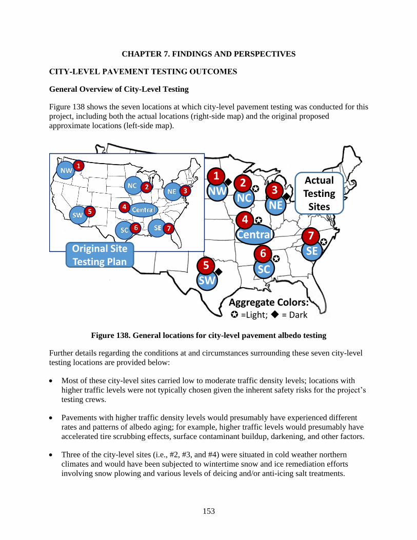
153

CHAPTER 7. FINDINGS AND PERSPECTIVES

CITY-LEVEL PAVEMENT TESTING OUTCOMES

General Overview of City-Level Testing

Figure 138 shows the seven locations at which city-level pavement testing was conducted for this

project, including both the actual locations (right-side map) and the original proposed

approximate locations (left-side map).

Figure 138. General locations for city-level pavement albedo testing

Further details regarding the conditions at and circumstances surrounding these seven city-level

testing locations are provided below:

• Most of these city-level sites carried low to moderate traffic density levels; locations with

higher traffic levels were not typically chosen given the inherent safety risks for the project’s

testing crews.

• Pavements with higher traffic density levels would presumably have experienced different

rates and patterns of albedo aging; for example, higher traffic levels would presumably have

accelerated tire scrubbing effects, surface contaminant buildup, darkening, and other factors.

• Three of the city-level sites (i.e., #2, #3, and #4) were situated in cold weather northern

climates and would have been subjected to wintertime snow and ice remediation efforts

involving snow plowing and various levels of deicing and/or anti-icing salt treatments.

1NW

2NC

3NE

5SW

6 NC7SE

4Central

SC

Original Site Testing Plan

ActualTesting

Sites

Aggregate Colors: =Light; ◆ = Dark

◆

◆

◆

154

• Three of the city-level sites (i.e., #5, #6, and #7) were situated in warm weather southern

climates and received little if any winter maintenance.

• One centrally situated site in Cape Girardeau, Missouri (#1), was considered to be a southern

city location and likely received little, if any, winter maintenance.

• The central site in Cape Girardeau, Missouri, was chosen as a midpoint between the

respective National CP Tech Center and NCAT home locations, and this site was

simultaneously evaluated in parallel by both testing teams to ensure the equivalence of the

teams’ testing results.

• Aggregate type and color were significant factors in choosing northern city-level sites (e.g.,

white limestone at South Bend, Indiana; beige-brown dolomite at Waterloo, Iowa; and pink

quartzite at Sioux Falls, South Dakota).

• Fewer PCC pavement options were available among the southern city-level testing locations;

as a result, aggregate type and color were problematic when choosing southern sites.

• There was an inevitable level of variability in pavement albedo measurements due a wide

range of factors and site-specific pavement surface changes (e.g., distress cracking, paint

striping, surface distress, albedometer tripod shadowing, varied sky clouding, or varied sky

hazing); even with extremely clear skies and in completely sunny testing periods, there was a

nominal ~0.5% to 1% degree of variability, and 2% to 3% variability was not uncommon.

City-Level Pavement Albedo Results

Overall Albedo Aging Behavior

Figure 139 provides a visual summary of the AC (black squares) and PCC (gray circles)

pavement albedo aging results observed during this project’s city-level testing effort.

155

black squares = AC, gray circles = PCC

Figure 139. Albedo aging results for AC and PCC pavements

The PCC pavement albedos started higher (i.e., between about 0.3 and 0.4) than the AC albedos

and tended to remain higher for the first 10 to 15 years of pavement life. Beyond 15 years of age,

the median for PCC pavement albedos was approximately 0.18. On the other hand, the AC

pavement albedos started lower (i.e., between about 0.07 and 0.14) than the PCC albedos and

tended to remain lower for the first 10 to 15 years of pavement life. Although relatively few AC

pavements with ages greater than 15 years were available for testing, the median for those results

was 0.15.

Qualitatively, these PCC and AC albedo aging results suggest a progressive period of

convergence over an approximately 15-year period. Further analysis of these albedo results in

terms of geographic location is provided below.

Specific PCC Albedo Aging Behavior

Figure 140 provides a further breakdown of PCC albedo aging results relative to geographic

location (with gray circles for northern locations and cross-hatched circles for southern

locations).

0.00

0.05

0.10

0.15

0.20

0.25

0.30

0.35

0.40

0 5 10 15 20 25 30 35 40

Albedo

Pavement Age (years)

PCC-All

AC-All

156

gray circles = northern locations, cross-hatched circles = southern locations

Figure 140. PCC albedo aging behavior relative to northern versus southern location

These results show that the four lowest measured albedos were all located at southern city sites,

and twelve southern sites and only eight northern sites had albedos of 0.25 or below. Conversely,

only four southern sites and seven northern sites had albedos above 0.25. This distribution

suggests that wintertime maintenance in northern locations may contribute to their higher albedo

levels, in that the mechanical abrasion of pavement surfaces during snow plowing activities may

be annually recleaning pavements by scraping, abrading, and physically cleaning previously

stained PCC pavements.

Specific AC Albedo Aging Behavior

Figure 141 provides a similar breakdown of AC albedo aging results relative to geographic

location (with solid black squares for northern locations and cross-hatched squares for southern

locations).

157

solid black squares = northern locations, cross-hatched squares = southern locations

Figure 141. AC albedo aging behavior relative to northern versus southern location

This figure shows an even more pronounced pattern of higher AC albedo results being observed

for the northern testing locations. Nine of the lowest albedo values were observed at southern

locations, while nine of the fifteen highest observed albedos were measured at northern cities.

Here again, this outcome again suggests that wintertime maintenance, and likely the mechanical

abrasion of pavement surfaces during snow plowing activities, may also be annually recleaning

AC pavements by mechanically scraping and cleaning exposed aggregate surfaces.

ALBEDO AGING FACTOR ASSESSMENT

After accruing multiple months of hands-on experience evaluating pavement albedos, it would

be fair to acknowledge that the cause-and-effect factors that appear to be linked with albedo

aging are both complex and overlapping. Even then, the perceived primary mechanisms for AC

albedo aging appear to be different than the main factors driving PCC albedo change. Table 30

provides a collated summary of the factors believed to be contributing to these changes.

158

Table 30. General summary of perceived aging effect mechanisms for pavement albedo aging

Factors Aging effect mechanisms

AC PCC

Low Med High Low Med High

Mastic binder (AC)

and mortar paste

(PCC) changes

Composition and color variations ⚫ ⚫

Supplementary material additions ⚫ ⚫

Solar insolation–induced heating (in relation to seasonal and

geographic variations) ⚫ ⚫

Solar insolation–induced photochemical oxidation (in relation

to seasonal and geographic variations) ⚫ ⚫

Coarse aggregate

changes

Traffic volume–related rolling-wheel erosion of mastic binder

or mortar paste leading to coarse aggregate exposure ⚫ ⚫

Chemical composition, glassiness, and color variations ⚫ ⚫

Fine aggregate

changes

Traffic volume–related rolling-wheel erosion of mastic or

mortar leading to fine aggregate exposure ⚫ ⚫

Chemical composition, glassiness, and color variations ⚫ ⚫

Mechanical scrubbing Traffic-related rolling-wheel mechanical scrubbing against

pavement surfaces ⚫ ⚫

Surface staining and

contamination

Physical contaminant deposition (e.g., tire crumb particulates,

soil, oil, antifreeze, or grease) ⚫ ⚫

Chemical reaction (e.g., acid-base, redox, precipitation,

chemical binding, or complexation) ⚫ ⚫

Biological fouling (attachment of microbial bacteria, algae,

fungus, mold, etc.) ⚫ ⚫

Construction changes Surface floating ⚫ ⚫

Surface brushing ⚫ ⚫

Surface tining ⚫ ⚫

Non-winter weather

exposure Rain-induced wetting and washing ⚫ ⚫

159

The factors are ranked within Table 30 according to the expected levels of effect, whether low,

medium, or high, for both AC and PCC pavement options.

Various combinations of the following three factors were believed to be the primary mechanisms

for AC albedo aging: (1) mastic binder degradation and erosion (i.e., via traffic or weathering or

photocatalytic degradation); (2) exposed coarse aggregate color, composition, and character; and

(3) winter maintenance effects.

As for PCC albedo aging, various combinations of the following five factors were believed to be

the primary mechanisms: (1) traffic-induced surface abrasion and weathering, (2) concrete paste

color and composition, (3) staining (chemical, physical, and biological), (4) surface roughness,

and (5) winter maintenance.

LABORATORY PAVEMENT CORE RESULTS


Figure 142 provides a direct comparison of PCC and AC thermal conductivity (k) results, which

were measured for cores removed from the city-level testing sites, in relation to other values

typically cited in the literature as well as the currently recommended NCHRP EICM values.

NCHRP citation: Zapata and Houston 2008

Figure 142. Core thermal conductivity results

Note that these results were obtained for dry pavement materials and that field materials with

higher moisture contents would have had significantly higher thermal conductivities (see the

discussion in Chapter 7 regarding pavement thermal modeling).

The following findings and perspectives regarding the observed core thermal conductivities are

warranted.

PCC Core Thermal Conductivities

• This project’s PCC cores exhibited a wide range of measured thermal conductivities (i.e.,

from 0.8 to 1.4 W/(m2•°C)).

0.8

Corlew (1968)

Benz (2001)

This study (ISU-2016)

This study(Auburn-2016)



Thermal Conductivity (W/m2-oC)(Reference ‘NCHRP’ = Zapata and Houston, 2008)

1.4

1.3

1.2

1.1

1.0

0.8

0.9

1.5

1.4

1.3

1.2

1.1

1.0

0.9

1.5PCC AC

160

• The northern PCC core k results tended to be lower than those measured in the southern

(NCAT) cores; this difference, however, may be attributable to differences in analytical

method (see the discussion in Chapter 5 and Appendix A).

• In general, the majority of the PCC core k results (and that of the frequently cited Bentz et al.

2001) are higher than the NCHRP EICM value cited by Zapata and Houston (2008).

• These variations suggest that a higher k value would be advisable during future NCHRP

EICM modeling.

AC Core Thermal Conductivities

• Here again, this project’s AC cores exhibited a wide range of measured thermal

conductivities (i.e., from 0.8 to 1.5 W/(m2•°C)).

• As with the southern PCC results, the southern AC core k results tended to be higher; while

this difference may also be attributable to inherent variations among aggregate materials and

properties, the research team’s general sense was that this variation was caused by

differences in analytical method (see the discussion in Chapter 5 and Appendix A).

• In general, this project’s AC core k results (and that of the frequently cited Corlew and

Dickson 1968), are similar to the NCHRP EICM value cited by Zapata and Houston (2008).

Specific Heat

Figure 143 provides a direct comparison of PCC and AC specific heat results, which were

measured for cores removed from the city-level testing sites, in relation to other values typically

cited in the literature as well as the currently recommended NCHRP EICM values.

NCHRP citation: Zapata and Houston 2008

Figure 143. Core specific heat results

Here again, as with the thermal conductivity findings, it must be noted that these results were

obtained for dry pavement materials and that field materials with higher moisture contents would

have had significantly higher specific heat capacities (see the discussion in Chapter 7 regarding

pavement thermal modeling).

The following findings and perspectives regarding this project’s observed core specific heat (SH)

values are warranted.

0.6

0.7

0.8

0.9

1.0

0.6

0.7

0.8

0.9

1.0Corlew (1968)

Benz (2001)





Specific Heat (kJ/kg-oC)(Reference ‘NCHRP’ = Zapata and Houston, 2008)

PCC AC

161

PCC Core Specific Heat

• This project’s PCC cores exhibited a wide range of measured specific heat values (i.e., from

0.6 to ~0.9 kJ/(kg•°C)).

• The northern PCC core k results tended to have a wider (and lower-end) range than those

measured for the southern (i.e., NCAT) cores. This difference may be attributable to

differences in analytical method (see the discussion in Chapter 5 and Appendix A), but they

may also be linked with variations in northern versus southern aggregate properties.

• In general, the majority of the PCC core k results (and that of the frequently cited Bentz et al.

2001), are substantially higher than the NCHRP EICM value cited by Zapata and Houston

(2008).

• These variations suggest that a higher SH estimate (e.g., ~0.75 to ~0.85 versus 0.63

kJ/(kg•°C)) would be advisable during future NCHRP EICM PCC modeling; this change

would conceptually increase the heat sorption capacity of the PCC materials by a significant

amount, to a level closer to that of AC pavements.

AC Core Specific Heat

• Here again, this project’s AC cores exhibited a wide range of measured specific heat values

(i.e., from 0.65 to ~0.95 kJ/(kg•°C)).

• As with the northern PCC results, the northern AC core SH results tended to have a wider

(and lower-end) range; here again, this difference may be attributable to differences in

analytical method (see the discussion in Chapter 5 and Appendix A), but they may also be

linked with variations in northern versus southern aggregate properties.

• In general, the majority of the AC core SH results (and that of the frequently cited Corlew

and Dickson 1968), are higher than the NCHRP EICM value cited by Zapata and Houston

(2008).

• In general, this project’s AC core SH results tended to be below both that of the NCHRP

EICM value cited by Zapata and Houston (2008) and that of the frequently cited Corlew and

Dickson (1968).

• This variation suggests that a lower SH estimate (e.g., ~0.8 versus 0.92 kJ/(kg•°C)) would be

advisable during future NCHRP EICM AC modeling; this change would conceptually

decrease the heat sorption capacity of the AC materials by a significant amount.

Emissivity

Figure 144 provides a direct comparison of PCC and AC emissivity (E) results, which were

measured for cores removed from the city-level testing sites, in relation to values cited in

Engineering ToolBox (2016c).

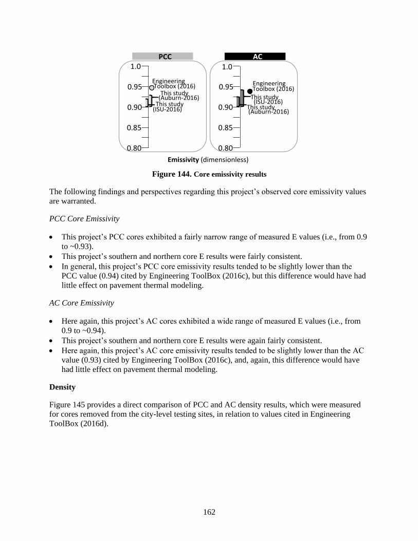
162

Figure 144. Core emissivity results

The following findings and perspectives regarding this project’s observed core emissivity values

are warranted.

PCC Core Emissivity

• This project’s PCC cores exhibited a fairly narrow range of measured E values (i.e., from 0.9

to ~0.93).

• This project’s southern and northern core E results were fairly consistent.

• In general, this project’s PCC core emissivity results tended to be slightly lower than the

PCC value (0.94) cited by Engineering ToolBox (2016c), but this difference would have had

little effect on pavement thermal modeling.

AC Core Emissivity

• Here again, this project’s AC cores exhibited a wide range of measured E values (i.e., from

0.9 to ~0.94).

• This project’s southern and northern core E results were again fairly consistent.

• Here again, this project’s AC core emissivity results tended to be slightly lower than the AC

value (0.93) cited by Engineering ToolBox (2016c), and, again, this difference would have

had little effect on pavement thermal modeling.

Density

Figure 145 provides a direct comparison of PCC and AC density results, which were measured

for cores removed from the city-level testing sites, in relation to values cited in Engineering

ToolBox (2016d).

Toolbox (2016)

This study 0.90

0.800.80

0.85

0.90

0.95

1.0

Toolbox (2016)

(ISU-2016)

(Auburn-2016)

PCC AC

Emissivity (dimensionless)

0.85

0.95

1.0

This study

Engineering

This study

This study(ISU-2016)

(Auburn-2016)

Engineering

163

Figure 145. Core density results

The following findings and perspectives regarding this project’s observed core density values are

warranted.

PCC Core Density

• This project’s PCC core densities ranged from ~2.0 to ~2.4 g/cm3.

• Both the northern and southern PCC core density results fell into the same range.

• In general, this project’s PCC core density results were comparable to the PCC values

(medium = 1.3–1.7 and high = 2.0–2.4) cited by Engineering ToolBox (2016d).

• This PCC density range was considerably higher than that observed for the AC core testing.

The higher range for the PCC cores was likely a function of aggregate density variability or

perhaps a function of variations in air entrainment among the PCC materials.

AC Core Density

• This project’s AC core densities ranged from ~2.2 to ~2.4 g/cm3.

• Here again, both the northern and southern AC core density results had about the same range.

• In general, this project’s AC core density results were comparable to the AC value

(compacted = 2.36) cited by Engineering ToolBox (2016d).

MODELING OUTCOMES

Pavement Albedo Model

The city-level testing results summarized in Chapter 7 show a distinct difference between PCC

albedo over time and AC albedo over time. A PCC surface has a high initial albedo trending to a

lower albedo over time, while an AC surface has a low initial albedo trending to a higher albedo

over time. While the data trends have some resemblance of being mirror images and appear to

merge after 15 years, the differences in the initial trends warrant the development of separate

albedo models. As the AC and PCC models were developed, the dominant variables for each

model were observed to be distinctly different. This finding further confirmed that the two

surface types require unique models.

2.5

2.3

2.2

2.3

2.4

2.5

2.0

2.1

2.2

2.4 This study (ISU-2016)




PCC AC

Density (g/cm3)

2.0

2.1

EngineeringToolbox (2016)

EngineeringToolbox (2016)

164

The first notable observations of the data were that (1) each test city generated a unique best fit

regression curve for each surface type, (2) the best fit curves had a similar shape, and (3) the

long-term trend values settled at different albedo levels. The trends are easily observed in Figure

88 for asphalt surfaces and Figure 102 for concrete surfaces in Chapter 6. While there is certainly

overlap among some individual measured data, the best fit regression curves suggest that the

albedo for a specific location is related to one or more variables associated with that location.

The key to model development was to identify the pavement characteristics that created the

differences between the trends for each pavement type. The analysis of asphalt pavement

characteristics revealed that pavement surface age and coarse aggregate color had a significant

influence on the albedo. Using these factors, the differences between the actual field-measured

albedos and model-computed albedos had a standard deviation of 0.029. This was comparable to

the standard deviation of the differences between the field-measured data and the best fit

regression for each city site, which was 0.026. The analysis of concrete pavement characteristics

was not as successful. The best model achieved in the analysis used pavement surface age,

pavement surface texture, and coarse aggregate color. The differences between the actual field-

measured albedos and model-computed albedos had a standard deviation of 0.057. The

differences between the field-measured data and the best fit regression for each city site,

however, had a standard deviation of 0.034. It was concluded that the variables measured in this

study did not capture one or more key PCC pavement characteristics.

Coarse aggregate color was a key variable in this study because coarse aggregate color becomes

a predominant feature on the pavement surface over time. The albedo model developed for AC

pavements confirmed that coarse aggregate color was a dominant factor in albedo and correlated

well with the field-measured albedo data. The albedo model for PCC pavements included coarse

aggregate color, but the model did not adequately compare to field-measured albedo data. Other

pavement features, such as fine aggregate color and cement mortar color, need to be examined to

improve the PCC albedo model.

The albedo model for AC pavements was developed and should be validated. A process for

measuring coarse aggregate color was developed as part of this study and provides a basis for

distinguishing between aggregate colors on a grayscale chart. Further improvement of the

process for quantifying aggregate color would improve the repeatability of the measure.

Pavement Thermal Model

This project’s pavement thermal model results provided estimates for both temperature and heat

flux level that were reasonably close to the actual measured values. Worst-case variations of ~3

to 5 °C between actual and modeled temperatures were observed at near-surface locations that

dynamically experienced the highest heat flux rates during peak summer insolation periods. Even

then, however, modeling results were generated for pavement, base, and subbase materials for

which dry-state thermodynamic properties (i.e., thermal conductivity and specific heat) were

assumed, and even slight moisture changes could have introduced this sort of inherent error.

In regards to further insights derived from these modeling efforts, the following observations are

offered for AC and PCC pavement options (based on modeling outcomes derived for MnROAD

pavement locations):

165

• The most extreme pavement temperature dynamics take place during summer months with

high solar insolation.

• AC pavements during hot, full-sun summer days reach peak surface temperatures above

50 °C and undergo a ~30+ °C diurnal temperature swing (i.e., dropping to ~25 °C) between

peak day and night temperatures. Under similar conditions, peak PCC surface temperatures

are significantly lower, in the mid-30s °C, and experience a diurnal temperature swing

roughly one-half that of AC pavements.

• The summertime day-night swing drops substantially for both AC and PCC pavements

within the first ~15 to 20 cm of the pavement depth, to about a ~25 °C nighttime minimum in

both cases.

• These high temperatures are far lower and these thermal swings are far smaller in magnitude

during wintertime conditions, when there are far lower levels of solar insolation energy being

absorbed.

• By about a 20 to 24 cm depth, the subbase temperature beneath both the AC and PCC

pavements reaches a stable point, with relatively little daily diurnal temperature variability.

• A critical step in generating an optimal pavement thermal model is to choose the initial

pavement, base, and subbase temperatures at which the model begins. Initial guesses were

sequentially refined by running repetitive model cycles so that more realistic initial

assumptions could be inserted. Slight initial errors in these assumed temperatures were then

corrected by the model over a period of 24 to 48 hours elapsed modeling time.

• The Microsoft Excel spreadsheet model developed for this project performed quite well, but

modeling pavement, base, and subbase temperatures over just a 10-day period involved file

sizes above 60 MB due to the large amount of one-minute-increment internal weather data

required for its operation. These large Excel file sizes required careful selection of

“Automatic” versus “Manual” options within the “Calculation Options” under the

“Formulas” tab so that changes in data and/or modeling equations could be made in a lump

sum fashion before activating the next calculation run.

It should also be noted that the observed level of error for this modeling approach escalated

significantly when freezing or wet-weather conditions were encountered. This effect stemmed

from inherent changes in the physical properties of the pavement, base, and subbase materials

that significantly altered their heat transfer and storage capacities. For example, pavement, base,

and subbase thermal conductivity levels can be expected to dramatically increase in parallel with

escalating moisture levels. This limitation in thermal modeling is well known within the

academic field of agricultural soil physics and is generally considered to be a significant

intellectual challenge, whose resolution was far beyond the capacity of this research project.

PAVEMENT DESIGN MODEL INTEGRATION OUTCOMES (PAVE ME)

The results of the thermal model developed as part of this study compared favorably with the

field-measured thermal characteristics of the pavement for dry parameters. The thermal model

was not designed to address the influence of moisture in the materials, nor the thermal

characteristics of frozen materials. The model was transferred into a conventional Microsoft

Excel spreadsheet platform. The research team determined that the model was most accurate

when the increment of time progression was one minute. The computing speed of the

spreadsheet platform was not sufficient for processing continuous thermal conditions for more

166

than 10 days. These limitations of the thermal model (material moisture, frozen material, and

computing speed) made it impossible to perform a direct side-by-side comparison to the EICM

model used in the Pave ME software. The study examined the effect of the material thermal

properties used in Pave ME as an alternative approach.

The sensitivity analysis examined the effect of three thermal properties (i.e., albedo, thermal

conductivity, and specific heat) on the predicted performance of three different pavement

sections (thick AC, thin AC, and concrete). As previously noted, this analysis was completed

using English units as per the involved Pave ME software requirements. The default Pave ME

albedo value is 0.15 (expressed as 0.85 absorption), and the study varied the albedo from 0.10 to

0.20. The default Pave ME thermal conductivity value is 0.67 BTU/(hr•ft•°F) (1.16 W/(m•K))

for an asphalt mixture, and the study varied the thermal conductivity from 0.4 to 1.0

BTU/(hr•ft•°F) (0.69 to 1.74 W/(m•K)). The default Pave ME thermal conductivity value is 1.25

BTU/(hr•ft•°F) (2.17 W/(m•K)) for concrete, and the study varied the thermal conductivity from

1.0 to 1.5 BTU/(hr•ft•°F) (1.74 to 2.6 W/(m•K)). The default Pave ME specific heat capacity

values are 0.23 BTU/(lb•°F) (0.96 kJ/(kg•°C)) for asphalt and 0.28 BTU/(lb•°F) (1.17

kJ/(kg•°C)) for concrete, and the study varied the specific heat value from 0.1 to 0.4 BTU/(lb•°F)

(0.4 to 1.6 kJ/(kg•°C)).

A summary of the sensitivity analysis is given in the Figure 137 in Chapter 6. The bar chart

shows that the specific heat capacity of an asphalt mixture has a 12% to 18% influence on the

predicted performance of asphalt pavements, specifically on rutting and top-down cracking. The

sensitivity analysis showed that all three thermal properties have as much as a 17% influence on

the predicted performance of concrete pavements. The analysis also showed that the Pave ME

cracking model is very sensitive to the concrete’s specific heat capacity.

Test procedures for measuring thermal conductivity and specific heat capacity of pavement

materials were improved based on the test procedures initially developed by Arizona State

University. Both tests use the same pavement core sample, and the sample can be tested multiple

times. This albedo study continued to refine the test procedures but revealed a number of

limitations that need further improvement. The tests should be refined and validated before they

are considered for standardization.

SUSTAINABILITY ADVOCACY AND RATING SYSTEM INTEGRATION

OUTCOMES

At the present time, there are no highway infrastructure sustainability rating systems that

quantitatively stipulate specific albedo criteria in relation to either “cool pavement” or “urban

heat island” goals. Program managers for two such systems, Greenroads and GreenPAVE, have

both indicated that they are aware of the albedo aging behaviors that occur with asphalt and

concrete pavements, but that they have intentionally chosen to pursue a narrative, qualitative

“cool pavement” goal comparable to that used by other rating systems (e.g., New York’s

GreenLITES, Illinois’s I-LAST, and ASCE’s now obsolete SIPRS plan).

It is also noteworthy that the most recent, and arguably the most comprehensively developed,

highway infrastructure sustainability system, i.e., FHWA’s INVEST, has not included either

“cool pavement” or “urban heat island” reduction outcomes. INVEST’s promotion of

167

sustainability goals addresses triple-bottom-line outcomes for highway projects and programs,

while at the same time it does not encourage, let alone require, the sort of quantitative analysis

and comparison approach that is far more commonly encouraged by the vast majority of other

sustainability rating methods.

Quantitative albedo criteria, however, are still being used within the LEED rating protocol (i.e.,

relative to vertical building systems) to evaluate the capture and release of solar energy of non-

roof hardscape (e.g., parking) surfaces, but even then only initial and three-year solar reflectance

(versus albedo) metric thresholds are identified. Attempts to contact LEED program managers in

writing and by email were unsuccessful. Given that this contact could not be established, further

clarification and dialogue with the U.S. Green Building Council could not be completed (e.g., to

ascertain their line of reasoning behind the decision to establish their reflectance criteria or

regarding their shift to considering a three-year aging period for solar reflection), and subsequent

knowledge regarding this project’s albedo aging findings could not be transferred.

This project’s guidance for sustainability rating systems and advocacy initiatives regarding the

future consideration of pavement reflectivity includes the following points:

• Pavements with low albedos (e.g., below 0.1) experience higher daytime peak surface

temperatures than pavements with sizably higher albedos (e.g., above 0.3), and 90% of solar

insolation is absorbed by a pavement with a 0.1 albedo versus 70% for a pavement with a 0.3

albedo (i.e., a ~29% increase); therefore, pavements with higher albedos would equate to

“cooler” pavements.

• However, pavement albedo is not a constant parameter; pavement albedos change over time,

and the values for asphalt and concrete tend to converge after a period of approximately 15

years.

• Quantitative stipulations for pavement systems regarding albedo criteria, therefore, are

complicated by this albedo variability, let alone the inherent uncertainty as to the exact

cause-and-effect correlation between specific albedo values and consequent UHI benefits.

• Qualitative stipulations for pavement systems, i.e., “cool pavement” and “urban heat island

reduction” outcomes, have consequently proven to be more widely favored within the

sustainability advocacy community, and pavement designers are encouraged to flexibly

pursue these goals on a conceptual basis.

ANALYTICAL OUTCOMES

Lessons Learned About Finding Host Cities and Site Selection

Finding host agencies proved to be more difficult than originally anticipated. The requirements

for a host agency summarized in Table 15 in Chapter 5 were effective for communicating the

research study’s requirements as well as acknowledging the demands on the host agency. Host

cities were identified from websites showing agency interest in sustainability. A number of

interested cities could not participate, however, due to their lack of PCC sites. Interest in varying

aggregate geology (aggregate color) was a key factor in host city selection, but the limited

availability of host cities did not produce a broad selection of color. Further field studies will

need to explore other methods for identifying host agencies with the desired site parameters.

168

The research team was very successful in coordinating with the host agencies to identify

candidate sites for field testing. Most candidate sites were limited to locations with lower traffic

volumes to minimize traffic disruption. Some four-lane sections with low to moderate traffic

were considered where a single lane closure still permitted reasonable traffic movement. This

coordination was particularly successful because 8 of the 10 sites required midday (non–rush

hour) lane use. Some sites were two-lane sections with very low traffic that did not require

flaggers.

After sites were identified and approved for the study and the field testing team was on site, the

field testing team only determined one site to be too hazardous for data collection due to traffic

conditions. There was no time to identify and coordinate an alternative site for this area. The

field testing team must thus always have the authority to assess the safety of the testing location

and cancel testing if the site is deemed unsafe. For future site selection the addition of alternative

sites could be considered, but these alternative sites would need to include at least two AC (one

newer surface and one older surface) and two PCC (within a similar age range) to cover all

alternative selection criteria.

The field testing plan was designed around a single one-week visit to collect field data at each

host agency location. On paper, the intended site conditions required clear skies and dry

pavement conditions, and some field trips were postponed due to unfavorable weather forecasts.

The requirement for clear and dry conditions for the entire five-day period was not met during

most field testing trips. Weather conditions, specifically cloud cover and rain, required some

modification of the testing plan, and some 10-hour site visits were shortened due to weather

conditions.

Lessons Learned About Field Site Testing

Pavement surface albedo, roughness, and color are key variables for albedo modeling. At least

30 minutes of albedo measurements should be collected so that the best 10- to 15-minute

increment can be used to determine the pavement surface albedo. Surface roughness should be

measured in the wheel path and in the centerline to capture any differences in surface polishing.

These differences may have an effect on the albedo value because albedo is measured within a

3.7 m radius, which includes both the center of the lane and the wheel paths. Pavement surface

color, like roughness, should be measured in both the wheel paths and center of the lane. Color

values are easy to obtain and can serve as a backup for reviewing and analyzing albedo

measurements. These values and the measured albedo are generally redundant, and pavement

surface color is not used in an albedo model.

Pavement, base, and subgrade temperature should only be measured when long-term monitoring

is needed to collect field data for validating a pavement thermal model. The time required to

collect sufficient field measurements for thermal modeling should be at least one week,

preferably longer. The 10-hour and 24-hour data collected during this study were not useful. The

continuous data collected at MnROAD, however, were useful. Procedures and devices used to

collect pavement, base, and subgrade temperature must only minimally alter the pavement, and

devices need to be properly secured to avoid damage. If thermal testing is extended over a period

of many days, the method of coring is less critical than for short-term testing. Dry coring is

preferred but is impractical for most field testing operations, while wet coring influences the

169

thermal properties of the pavement materials until the excess water dissipates. The method used

in this research to install a heat flux sensor was successful, but a better method of gluing the

sensor in place without losing thermal conductivity should be developed for more permanent

installations.

Lessons Learned About Laboratory Testing

Standard thermal property testing for materials is not practical for pavement field cores.

Pavement core test methods originally developed by ASU were refined or modified in this study

to achieve more practical test procedures. Problems were encountered during the initial use of

the tests, and some issues were not resolved. For example, the core heater for the thermal

conductivity test did not generate uniform heat along the entire metal element shaft. A better core

heater should be considered for further testing.

The filler material for the thermal conductivity test was changed from the initial plan. The

thermal paste used by ASU was difficult to work with, and the thermal pads used by ASU

changed conductivity when compressed. Thermal grease was also difficult to work with,

particularly in cleaning the core for subsequent testing. The use of fine sand proved to be more

practical, but this material absorbed moisture and thus created variations in the level of saturation

during the progression of the test. A very thin coating of grease in the hole was used to mitigate

the absorption issue.

The hole drilled in the cores for the thermal conductivity test was reduced in diameter to obtain a

longer thermal conductivity path radially from the hole wall to the outer core surface. However,

drilling a straight hole using a smaller masonry drill bit proved very difficult. ASU used a larger

core bit instead of a drill bit to solve this problem, but this method decreased the radial thermal

conductivity path. To compensate for the hole offset, additional external surface temperature

sensors were used to get a reasonable average external temperature.

Problems were also encountered in preparing cores for testing. In some cases, the AC or PCC

material was too weak to drill without damaging the entire core. Some of the AC and PCC

materials were produced with very hard aggregates that could not be drilled successfully. In

either case, i.e., with weak material or very hard aggregate, some cores could not be prepared

and subsequently tested. When asphalt cores obtained from the field were shorter than the 5 in.

testing length, two cores were trimmed and bound together using asphalt binder to achieve the

length required for testing. Stacking cores for testing did not affect the testing because the

thermal energy movement in the test core is radial, not parallel to the core axis.

Using the core from the thermal conductivity test for the specific heat capacity test improved the

latter test. The drilled hole in the center of the core provided another surface for heat transfer and

thus reduced the time to achieve heat transfer to the water bath. A lower heat transfer time and

good chamber insulation improved the accuracy of the test. The water circulation system was

adequate, but other more effective systems should be identified.

The density of each core was measured after the core was prepared for testing, and very basic

external measurements were taken to determine the core volume. Future testing should perform

170

density testing before the cores are prepared for thermal testing using more appropriate test

methods.

A grayscale method for measuring pavement surface and aggregate color was developed as part

of this study. This method is dependent on proper lighting for photographing the core along with

the grayscale standard. Some of the photographs taken for this project showed a glare along the

side of the grayscale standard, which distorted the grayscale pattern. Improvements in the

lighting would improve the ability to properly select the grayscale value. This study measured

the color of the dominant coarse aggregate but provided no instruction for establishing the color

rating when the material was composed of mixed aggregate colors, such as for river gravel

sources. Because coarse aggregate color is a parameter of the albedo model for asphalt pavement

surfaces, a refined test procedure for surface mixtures with mixed coarse aggregate colors should

be developed.

RECOMMENDED FURTHER RESEARCH

Validation of Albedo Model for Asphalt Pavements

Validate the albedo model by repeating the field albedo measurements on another diverse group

of locations and pavement ages and compare the results obtained to the results of the asphalt

albedo prediction model developed in this study. Finding host cities should be much easier if the

study is limited to asphalt pavement surfaces, 15-minute albedo measurements, and one core.

The core is needed to obtain the coarse aggregate grayscale value and is a permanent record of

each test surface.

Broaden the PCC Pavement Surface Albedo Investigation

Examine the data and cores from this study to identify other key pavement surface characteristics

that influence PCC albedo. The research team believes the following PCC pavement roughening

methods and effects should be examined: (a) tining depth and orientation, (b) biological

mechanisms of surface discoloring (mold/algae), (c) roughness-related effects resulting from

winter maintenance activities, and (d) cement paste and mastic color (which remains exposed as

the pavement surface ages).

Wet and Frozen Pavement Thermal Modeling Investigation

Further research in relation to pavement thermal modeling under wet and freezing conditions

could be highly valuable, assuming that this effort can be successful. This challenge is already

being addressed to some extent within the agriculture-focused realm of soil physics, and

collaborative integration of both the agriculture-related and pavement-related efforts is highly

recommended.

Pavement Aggregate Material Characteristics Investigation

Further research in relation to aggregate properties and associated albedo reflectivity properties

is recommended and should cover the following: (1) the silica aspect and glassy reflectivity

(neither of which are captured by the grayscale measurement approach used for this project) and

171

(2) angularity versus rounded characteristics (which are also not captured by the MTD value

measured for this project).

Advancement of the Testing Protocols for Measuring Pavement Core Thermal Properties

This study identified numerous challenges in measuring the thermal conductivity and specific

heat capacity of pavement cores. Improvements to the tests are needed to increase the accuracy

of the measured values. Additional research should include measurements of standard materials

that have thermal properties similar to those AC and PCC materials tested and for which the

sample size is comparable to a pavement core.

173

REFERENCES

American Concrete Pavement Association (ACPA). (2002). Albedo: a measure of pavement

surface reflectance. American Concrete Pavement Association, Rosemont, IL.

www.acpa.org/.

Akbari, H., and Levinson, R. M. (2008). Status of cool roof standards in the United States.

Lawrence Berkeley National Laboratory, University of California, Berkeley, CA. June 23,

2008.

Akbari, H., Levinson, R., and Berdahl, P. (1996). ASTM Standards for Measuring Solar

Reflectance and Infrared Emittance of Construction Materials and Comparing their Steady-

State Surface Temperatures. ACEEE Summer Study on Energy Efficiency in Buildings, 1–9.

Akbari, H., Levinson, R., and Stern, S. (2008). Procedure for measuring the solar reflectance of

flat or curved roofing assemblies. Solar Energy, 82(7), 648–655.

doi.org/10.1016/j.solener.2008.01.001.

Alavi, M. Z, Pouranian, M. R., and Hajj, E. Y. (2014). Prediction of Asphalt Pavement

Temperature Profile with Finite Control Volume Method. Transportation Research Record:

Journal of the Transportation Research Board, No. 2456, pp. 96–106. DOI: 10.3141/2456-

10.

Asaeda, T., and Ca, V. T. (2000). Characteristics of permeable pavement during hot summer

weather and impact on the thermal environment. Building and Environment, 35(4), 363–375.

doi.org/10.1016/S0360-1323(99)00020-7.

Asaeda, T., Ca, V. T., and Wake, A. (1996). Heat storage of pavement and its effect on the lower

atmosphere. Atmospheric Environment, 30(3), 413–427. doi.org/10.1016/1352-

2310(94)00140-5.

Asaeda, T., and Ca, V. T. (1993). The subsurface transport of heat and moisture and its effect on

the environment: A numerical model. Boundary-Layer Meteorology, 65(1-2), 159–179.

doi.org/10.1007/BF00708822.

American Society of Heating, Refrigerating, and Air-Conditioning Engineers (ASHRAE).

(2003). Chapter 33: Solar Energy Use. Applications Handbook (SI). American Society of

Heating Refrigerating and Air-Conditioning Engineers, Atlanta, GA.

ASTM International. (2015). E1918-06: Standard Test Method for Measuring Solar Reflectance

of Horizontal and Low-Sloped Surfaces in the Field. ASTM International, West

Conshohocken, PA

ASTM International. (2014). C1549-09(2014): Standard Test Method for Determination of Solar

Reflectance Near Ambient Temperature Using a Portable Solar Reflectometer. ASTM

International, West Conshohocken, PA.

Bentz, D. P., Ehlen, M. A., Ferraris, C. F., and Graboczi, E. J. (2001). Sorptivity-based service

life predictions for concrete pavements. 7th International Conference on Concrete

Pavements (ICCP): The Use of Concrete in Developing Long-Lasting Pavement Solutions for

the 21st Century 1: 181-193. ciks.cbt.nist.gov/~ferraris/PDF/iccppaper.pdf.

Berdahl, P., Akbari, H., Levinson, R., Jacobs, J., Klink, F., and Everman, R. (2012). Three-year

weathering tests on asphalt shingles: Solar reflectance. Solar Energy Materials and Solar

Cells, 99, 277–281. doi.org/10.1016/j.solmat.2011.12.010.

Berdahl, P., Akbari, H., Jacobs, J., and Klink, F. (2008a). Surface roughness effects on the solar

reflectance of cool asphalt shingles. Solar Energy Materials and Solar Cells, 92(4), 482–489.

doi.org/10.1016/j.solmat.2007.10.011.

174

Berdahl, P., Akbari, H., Levinson, R., and Miller, W. A. (2008b). Weathering of roofing

materials - An overview. Construction and Building Materials, 22(4), 423–433.

doi.org/10.1016/j.conbuildmat.2006.10.015.

Berdahl, P., Akbari, H., and Rose, L. S. (2002). Aging of reflective roofs: soot deposition.

Applied Optics, 41(12), 2355–60. doi.org/10.1364/AO.41.002355.

Berdahl, P., and Fromberg, R. (1982). The Thermal Radiance of Clear Skies. Solar Energy,

29(4), 299–314.

Brown, H., Caputo Jr., S.A., Carnahan, K., and Nielsen, S. (2005). High Performance

Infrastructure Guidelines, October 2005. New York City Department of Design and

Construction, New York, NY.

Cambridge Systematics, Inc. (2005). Cool Pavement Report: EPA Cool Pavements Study,

Task 5. Cambridge Systematics, Inc., Chevy Chase, MD.

Carlson, J. D., Bhardwaj, R., Phelan, P. E., Kaloush, K. E., and Golden, J. S. (2010).

Determining Thermal Conductivity of Paving Materials Using Cylindrical Sample Geometry.

Journal of Materials in Civil Engineering, 22(2), 186–195. doi.org/10.1061/(ASCE)0899-

1561(2010)22:2(186).

Coakley, J. A. (2003). Reflectance and Albedo, Surface. Encyclopedia of Atmospheric Sciences.

Elsevier Science Ltd. pp. 1914–1923. doi.org/10.1016/B0-12-227090-8/00069-5.

Cole-Parmer. (2016). Emissivity of Specific Materials. Cole-Parmer Instrument Company, LLC.

Vernon Hills, IL. www.coleparmer.com/TechLibraryArticle/254.

Cool Roof Rating Council. (2016). About CRRC. Cool Roof Rating Council. Oakland, CA.

coolroofs.org/about-crrc/overview.

Corlew, J. S. and Dickson, P. F. (1968). Methods for Calculating Temperature Profiles of Hot-

Mix Asphalt Concrete as Related to the Construction of Asphalt Pavements. Association of

Asphalt Paving Technologists Proceedings, 37, 101–140.

Dempsey, B. J., Herlach, W. A., and Patel, A. J. (1985). The Climatic-Material-Structural

Pavement Analysis Program, Volume 3. Final Report FHWA/RD-84/115. Federal Highway

Administration, Washington DC.

Desjarlais, A. O., Petrie, T. W., Miller, W., Gillenwater, R., and Roodvoets, D. (2006).

Evaluating the energy performance of ballasted roof systems. Research in Building Physics

and Building Engineering, 473–478.

Devices and Services Company. (2014). Solar Spectrum Reflectometer. Devices and Services

Company, Dallas, TX. www.devicesandservices.com/prod01.htm.

Dolce, R. (2012). ISO-9060 Standard & Pyranometer Measurement Accuracy. American Solar

Energy Society World Renewable Energy Forum, Denver, CO, May 13–17, 2012.

ases.conference-services.net/resources/252/2859/pres/SOLAR2012_0829_presentation.pdf.

Engineering ToolBox. (2016a). Thermal Conductivity of Some Common Materials and Gases.

www.engineeringtoolbox.com/thermal-conductivity-d_429.html.

Engineering ToolBox. (2016b). Solids – Specific Heats. www.engineeringtoolbox.com/specific-

heat-solids-d_154.html.

Engineering ToolBox. (2016c). Emissivity Coefficients of Some Common Materials.

www.engineeringtoolbox.com/emissivity-coefficients-d_447.html.

Engineering ToolBox. (2016d). Concrete – Properties. www.engineeringtoolbox.com/concrete-

properties-d_1223.html.

175

Gaffin, S. R., Imhoff, M., Rosenzweig, C., Khanbilvardi, R., Pasqualini, A., Kong, A. Y. Y.,

Grillo, D., Freed, A., Hillel, D., and Hartung, E. (2012). Bright is the new black—multi-year

performance of high-albedo roofs in an urban climate. Environmental Research Letters, 7(1),

14029. doi.org/10.1088/1748-9326/7/1/014029.

Garcia, A., Hassn, A., Chiarelli, A., and Dawson, A. (2015). Multivariable analysis of potential

evaporation from moist asphalt mixture. Construction and Building Materials, 98, 80–88.


Gartland, L. M., Konopacki, S. J., and Akbari, H. (1996). Modeling the Effects of Reflective

Roofing. Paper presented at the 1996 American Council for an Energy-Efficiency Economy

(ACEEE) Summer Study on Energy Efficiency in Buildings, Pacific Grove, CA, August 25–

31, 1996.

Gui, J., Phelan, P., Kaloush, K., and Golden, J. (2007). Impact of Pavement Thermophysical

Properties on Surface Temperatures. Journal of Materials in Civil Engineering, 19(8), 683–

690. doi.org/10.1061/(ASCE)0899-1561(2007)19:8(683).

Guntor, N. A. A., Md Din, M. F., Ponraj, M., and Iwao, K. (2014). Thermal Performance of

Developed Coating Material as Cool Pavement Material for Tropical Regions. Journal of

Materials in Civil Engineering, 26(4), 755–760. doi.org/10.1061/(ASCE)MT.1943-

5533.0000859.

Hage, J. C. H. van der. (1992). Interpretation of Field Measurements Made with a Portable

Albedometer. Journal of Atmospheric and Oceanic Technology, 9(4), 420-425.

Hajj, E. Y., Sebaaly, P. E., Alavi, M. Z., and Morian, N. E. (2015). Evaluation of Thermal

Cracking Resistance of Asphalt Mixtures. Draft Final Report, Contract No. DTFH61-07-H-

00009, Federal Highway Administration, Washington, DC.

Hall, M., Dehdezi, P., Dawson, A., Grenfell, J., and Isola, R. (2012). Influence of the

Thermophysical Properties of Pavement Materials on the Evolution of Temperature Depth

Profiles in Different Climatic Regions. Journal of Materials in Civil Engineering, 24(1), 32–

47. doi.org/10.1061/(ASCE)MT.1943-5533.0000357.

Han, R., Jin, X., and Glover, C. (2011). Modeling Pavement Temperature for Use in Binder

Oxidation Models and Pavement Performance Prediction. Journal of Materials in Civil

Engineering, 23(4) (April), 351–359. doi.org/10.1061/(ASCE)MT.1943-5533.0000169.

Harvey, J., Kendall, A., Santero, N., Van Dam, T., Lee, I. S., and Wang, T. (2011). Pavement

Life Cycle Assessment Workshop, May 5–7, 2010 in Davis, California, USA. International

Journal of Life Cycle Assessment, 16(944). doi.org/10.1007/s11367-011-0334-2.

Hassn, A., Chiarelli, A., Dawson, A., and Garcia, A. (2016). Thermal properties of asphalt

pavements under dry and wet conditions. Materials & Design, 91, 432–439.

doi.org/10.1016/j.matdes.2015.11.116.

Hendel, M., Colombert, M., Diab, Y., and Royon, L. (2015). An analysis of pavement heat flux

to optimize the water efficiency of a pavement-watering method. Applied Thermal

Engineering, 78, 658–669. doi.org/10.1016/j.applthermaleng.2014.11.060.

Herb, W. R., Janke, B., Mohseni, O., and Stefan, H. G. (2009). Runoff Temperature Model for

Paved Surfaces. Journal of Hydrologic Engineering, 14(10), 1146–1155.

doi.org/10.1061/(ASCE)HE.1943-5584.0000108.

Herb, S., Marasteanu, M., and Stefan, H. G. (2006). Simulation and Characterization of Asphalt

Pavement Temperatures. Minnesota Department of Transportation, St. Paul, MN.

176

Hermansson, Å. (2001). Mathematical Model for Calculation of Pavement Temperatures.

Transportation Research Record: Journal of the Transportation Research Board, No. 1764,

180–188.

Ho, C.-H. and Romero, P. (2009). Low Design Temperatures of Asphalt Pavements in Dry–

Freeze Regions: Predicting by Means of Solar Radiation, Transient Heat Transfer, and Finite

Element Method. Transportation Research Record: Journal of the Transportation Research

Board, No. 2127, 60–71.

Kaloush, K. E., Carlson, J. D., Golden, J. S., and Phelan, P. E. (2008). The Thermal and

Radiative Characteristics of Concrete Pavements in Mitigating Urban Heat Island Effects.

Portland Cement Association, Skokie, IL.

Kenward, A., Yawitz, D., Sanford, T., and Wang, R. (2014). Summer in the City: Hot and

Getting Hotter. Climate Central, Princeton, NJ. assets.climatecentral.org/pdfs/UHI-

AppendixC.pdf.

Kertesz, R. and Sansalone, J. (2014). Hydrologic Transport of Thermal Energy from Pavement.

Journal of Environmental Engineering, 140(8), 4014028. doi.org/10.1061/(ASCE)EE.1943-

7870.0000831.

Kim, K., Thompson, A. M., and Botter, G. (2008). Modeling of thermal runoff response from an

asphalt-paved plot in the framework of mass response functions. Water Resources Research,

44(11).

Kinouchi, T., Yoshinaka, T., Fukae, N., and Kanda, M. (2004). Development of Cool Pavement

with Dark Colored High Albedo Coating. Paper presented at the Fifth Conference on Urban

Environment. Vancouver, BC, August 23, 2004. www.coolrooftoolkit.org/wp-

content/uploads/2012/04/High-Reflective-Pavement-PWRI-Nippo-Tokyo-Tech.pdf.

Kipp & Zonen. (2016a). The Working Principle of a Thermopile Pyranometer. Kipp & Zonen

B.V., Delft, The Netherlands. www.kippzonen.com/News/572/The-Working-Principle-of-a-

Thermopile-Pyranometer#.VvHUJ6crK70.

Kipp & Zonen. (2016b). CMA6 Albedometer. Kipp & Zonen B.V., Delft, The Netherlands.

www.kippzonen.com/Product/22/CMA-6-Albedometer#.VvHXeacrK70.

Kipp & Zonen. (2013). Instruction Manual: CMP/CMA series. Kipp & Zonen B.V. Delf, The

Netherlands.

Levinson, R. (2012). The case for cool roofs. Lawrence Berkeley National Laboratories,

University of California, Berkeley, CA. heatisland.lbl.gov/publications/case-cool-roofs.

Levinson, R., Akbari, H., and Berdahl, P. (2010a). Measuring solar reflectance – Part I: Defining

a metric that accurately predicts solar heat gain. Solar Energy, 84(9), 1717–1744.

doi.org/10.1016/j.solener.2010.04.018.

Levinson, R., Akbari, H., and Berdahl, P. (2010b). Measuring solar reflectance – Part II: Review

of practical methods. Solar Energy, 84(9), 1745–1759.

doi.org/10.1016/j.solener.2010.04.017.

Levinson, R. (2009). Advances in Measuring Solar Reflectance, or, why that roof isn't it as cool

as you thought it was. Scientist (June), 1–40.

Levinson, R., Berdahl, P., Akbari, H., Miller, W. Joedicke, I., Reilly, J., Suzuki, Y., and

Vondran, M. (2007). Methods of creating solar-reflective nonwhite surfaces and their

application to residential roofing materials. Solar Energy Materials and Solar Cells, 91(4),

304–314. doi.org/10.1016/j.solmat.2006.06.062.

177

Levinson, R., Berdahl, P., Asefaw Berhe, A., and Akbari, H. (2005a). Effects of soiling and

cleaning on the reflectance and solar heat gain of a light-colored roofing membrane.

Atmospheric Environment, 39(40), 7807–7824. doi.org/10.1016/j.atmosenv.2005.08.037.

Levinson, R., Berdahl, P., Asefaw Berhe, A., and Akbari, H. (2005b). Solar spectral optical

properties of pigments – Part I: model for deriving scattering and absorption coefficients

from transmittance and reflectance measurements. Solar Energy Materials and Solar Cells,

89(4), 319–349.

Levinson, R. and Akbari, H. (2002). Effects of composition and exposure on the solar reflectance

of portland cement concrete. Cement and Concrete Research, 32(11), 1679–1698.

doi.org/10.1016/S0008-8846(02)00835-9.

Li, H., C., Harvey, J., He, Y., and Li, P. (2015). Pavement Treatment Practices and Dynamic

Albedo Change of Urban Pavement Network in California. Paper presented at the 2015

Annual Meeting of the Transportation Research Board, Washington, DC, January 11–15,

2015.

Li, H., He, Y., and Harvey, J. (2014). Cool Pavement Strategies for Enhancing Urban

Sustainability. Paper presented at the 7th Geotechnical Graduate Student Society at UC

Davis Round Table, Davis, CA, April 18, 2014.

Li, H., Harvey, J., and Kendall, A. (2013a). Field measurement of albedo for different land cover

materials and effects on thermal performance. Building and Environment, 59, 536–546.

doi.org/10.1016/j.buildenv.2012.10.014.

Li, H., Harvey, J. T., Holland, T. J., and Kayhanian, M. (2013b). Corrigendum: The use of

reflective and permeable pavements as a potential practice for heat island mitigation and

stormwater management. Environmental Research Letters, 8(4), 049501.

doi.org/10.1088/1748-9326/8/4/049501

Lin, Y. and Ichinose, T. (2015). Experimental evaluation of mitigation of thermal effects by

“Katsuren Travertine” paving material. Energy and Buildings, 81, 253–261.

Lin, T., Matzarakis, A., Hwang, R., and Huang, Y. (2010). Effect of pavements albedo on long-

term outdoor thermal comfort. Paper presented at the 7th Conference on Biometeorology,

Freiburg, Germany, April 12–14, 2010.

Liu, C. and Gazis, D. (2001). Heat Conduction Waves in Bilayer Cement Concrete Structures.

Journal of Engineering Mechanics, 127(11), 1195–1198. doi.org/10.1061/(ASCE)0733-

9399(2001)127:11(1195).

Lytton, R. L., Uzan, J., Femando, E. G., Roque, R., Hiltunen, D., and Stoffels, S. M. (1993).

Development and Validation of Performance Prediction Models and Specifications for

Asphalt Binders and Paving Mixes. Final Report SHRP-A357. Strategic Highway Research

Program, Washington DC.

Mallick, R. B., Worsman, R. K., Li, H., Harvey, J., and Bhowmick, S. (2014). Effective

reduction of asphalt pavement temperatures. Asphalt Pavements. Taylor and Francis,

London, 1409–1420.

Marasteanu, M., Velasquiez, R., Herb, W., Tweet, J., Turos, M., Watson, M., and Stefan, H.

(2008). Determination of Optimum Time for the Application of Surface Treatments to Asphalt

Concrete Pavements - Phase II. MN/RC 2008-16. Minnesota Department of Transportation,

St. Paul, MN.

Marceau, M. L. and VanGeem, M. G. (2007). Solar Reflectance of Concretes for LEED

Sustainable Sites Credit: Heat Island Effect. PCA R&D Serial No. 2982. Portland Cement

Association, Skokie, IL.

178

Menon, S., Levinson, R., Fischer, M., Millstein, D., Brown, N., Salamanca, F., Sednev, I., and

Rosenfeld, A. (2011). Cool Roofs and Global Cooling: Concerns about study by Jacobson

and Ten Hoeve. Lawrence Berkeley National Laboratories, University of California,

Berkeley, CA.

Mikron Instrument Company, Inc. (n.d.). Table of Emissivity of Various Surfaces. Mikron

Instrument Company, Inc. Schaffhausen, Switzerland. www-

eng.lbl.gov/~dw/projects/DW4229_LHC_detector_analysis/calculations/emissivity2.pdf.

Mills, G. (2008). Luke Howard and The Climate of London. Weather, 63(6), 153–157.

doi.org/10.1002/wea.195.

Minhoto, M. J. C., Pais, J. C., Pereira, P. A. A., and Picado-Santos, L. G. (2005). Predicting

Asphalt Pavement Temperature with a Three-Dimensional Finite Element Method.

Transportation Research Record: Journal of the Transportation Research Board, No. 1919,

96–110.

Mohseni, A. (1998). LTPP Seasonal Asphalt Concrete (AC) Pavement Temperature Models

(Vol. 7). Federal Highway Administration, Long-Term Pavement Performance Program,

McLean, VA.

Oleson, K. W., Bonan, G. B., and Feddema, J. (2010). Effects of white roofs on urban

temperature in a global climate model. Geophysical Research Letters, 37.

doi.org/10.1029/2009GL042194.

Parker, D. S., Huang, Y. J., Konopacki, S. J., Gartland, L. M., Sherwin, J. R., and Gu, L. (1998).

Measured and simulated performance of reflective roofing systems in residential buildings.

ASHRAE Transactions, 104(Pt 1B), 963–975.

Pomerantz, M., Akbari, H., Levinson, R., and Pon, B. (2005). Reflective Pavements and the

Urban Heat Island Effect. Paper presented at Cool Pavements: Developing Research and

Implementation Strategies Workshop, Washington, DC, June 27, 2005.

Pomerantz, M., Akbari, H., and John, T. (2000). Cooler Reflective Pavements Give Benefits

Beyond Energy Savings: Durability and Illumination. ACEEE 2000 Summer Study on Energy

Efficiency in Buildings, 8, 293–304.

Pomerantz, M., Akbari, H., Chen, A., Taha, H., and Rosenfeld, A. H. (1997). Pavement

Materials for Heat Island Mitigation. Report LBL-38074. Lawrence Berkeley National

Laboratory, University of California, Berkeley, CA.

Puttonen, E., Suomalainen, J., Hakala, T., and Peltoniemi, J. (2009). Measurement of reflectance

properties of asphalt surfaces and their usability as reference targets for aerial photos. IEEE

Transactions on Geoscience and Remote Sensing, 47(7), 2330–2339.

doi.org/10.1109/TGRS.2008.2010132.

Qin, Y., and Hiller, J. E. (2014). Understanding pavement-surface energy balance and its

implications on cool pavement development. Energy and Buildings, 85, 389–399.

doi.org/10.1016/j.enbuild.2014.09.076.

Qin, Y., and Hiller, J. E. (2011). Modeling temperature distribution in rigid pavement slabs:

Impact of air temperature. Construction and Building Materials, 25(9), 3753–3761.


Richard, C., Dore, G., Lemieux, C., Bilodeau, J.-P., and Haure-Touzé, J. (2015). Albedo of

Pavement Surfacing Materials: In Situ Measurements. Cold Regions Engineering:

Developing and Maintaining Resilient Infrastructure, 181–192.

doi.org/10.1061/9780784479315.017.

179

RJC Solutions. (2016). Roger Johnson Consulting Ltd. Langley, BC.

www.rjcsolutions.com/calculators/grav-den.html.

Rymer, B. and Levine, K.K. (2011). Cool Pavements Research and Technology. California

Department of Transportation, Division of Research and Innovation, Sacramento, CA.

Sansalone, J. J., and Teng, Z. (2005). Transient rainfall-runoff loadings to a partial exfiltration

system: Implications for urban water quantity and quality. Journal of Environmental

Engineering, 131(8), 1155–1167. doi.org/10.1061/(ASCE)0733-9372(2005)131:8(1155).

Santamouris, M., Synnefa, A., and Karlessi, T. (2011). Using advanced cool materials in the

urban built environment to mitigate heat islands and improve thermal comfort conditions.

Solar Energy, 85(12), 3085–3102. doi.org/10.1016/j.solener.2010.12.023.

Sarat, A.-A. and Eusuf, M. A. (2012). Effects of Pavement Surface Temperature on the

Modification of Urban Thermal Environment. Journal of Architecture and Built

Environment, 39(1), 1–4.

Sen, S. (2015). Impact of Pavements on the Urban Heat Island. MS thesis, University of Illinois

at Urbana-Champaign, IL.

Sen, S., King, D., and Roesler, J. (2015). Structural and Environmental Benefits of Concrete

Inlays for Pavement Preservation. Airfield and Highway Pavements 2015, 697–707.

doi.org/10.1061/9780784479216.062.

Solaimanian, J., and Kennedy, T. W. (1993). Predicting Maximum Pavement Surface

Temperature Using Maximum Air Temperature and Hourly Solar Radiation. Transportation

Research Record: Journal of the Transportation Research Board, No. 1417, 1–11.

Taha, H. (1997). Urban climates and heat islands: albedo, evapotranspiration, and anthropogenic

heat. Energy and Buildings, 25(2), 99–103. doi.org/10.1016/S0378-7788(96)00999-1.

Taha, H., Sailor, D., and Akbari, H. (1992). High-Albedo Materials for Reducing Building

Cooling Energy Use. Energy. doi.org/10.2172/7000986.

Taha H., Konopacki, S., and Gabersek, S. (1999). Impacts of large-scale surface modifications

on meteorological conditions and energy use: a 10-region modeling study. Theoretical and

Applied Climatology, 62, 175–85.

Takebayashi, H. and Moriyama, M. (2012). Study on surface heat budget of various pavements

for urban heat island mitigation. Advances in Materials Science and Engineering, Vol. 2012.

doi.org/10.1155/2012/523051.

Tan, S.-A. and Fwa, T.-F. (1992). Influence of pavement materials on the thermal environment

of outdoor spaces. Building and Environment, 27(3), 289–295. doi.org/10.1016/0360-

1323(92)90030-S.

Thompson, A. M., Kim, K., and Vandermuss, A. J. (2008). Thermal characteristics of

stormwater runoff from asphalt and sod surfaces. Journal of the American Water Resources

Association, 44(5), 1325–1336. doi.org/10.1111/j.1752-1688.2008.00226.x.

Tran, N., Powell, B., Marks, H., West, Kvasnak, A. (2009). Strategies for Design and

Construction of High - Reflectance Asphalt Pavements. Transportation Research Record:

Journal of the Transportation Research Board, 2098, 124–130.

U.S. Environmental Protection Agency (U.S. EPA). (2008a). Cool Roofs. Reducing Urban Heat

Islands: Compendium of Strategies. U.S. Environmental Protection Agency Office of

Atmospheric Programs Climate Protection Partnership Division.

www.epa.gov/sites/production/files/2014-06/documents/coolroofscompendium.pdf.

180

U.S. Environmental Protection Agency (U.S. EPA). (2008b). Heat Island Reduction Activities.

Reducing Urban Heat Islands: Compendium of Strategies.U.S. Environmental Protection

Agency Office of Atmospheric Programs Climate Protection Partnership Division.

www.epa.gov/sites/production/files/2014-06/documents/activitiescompendium.pdf.

U.S. Environmental Protection Agency (U.S. EPA). (2003). Cooling Summertime Temperatures:

Strategies to Reduce Urban Heat Islands. Environmental Protection Agency, Washington,

DC. www.epa.gov/sites/production/files/2014-06/documents/hiribrochure.pdf.

University of Nevada, Reno. (2014). Asphalt Research Consortium. Free Software (TEMPS).

www.arc.unr.edu/Software.html#TEMPS&_ga=2.238670720.1215785763.1502206793-

2032091559.1502206793.

Van Buren, M. A., Watt, W. E., Marsalek, J., and Anderson, B. C. (2000). Thermal enhancement

of stormwater runoff by paved surfaces. Water Research, 34(4), 1359–1371.

doi.org/10.1016/S0043-1354(99)00244-4.

Vehrencamp, J. E. (1953). Experimental Investigation of Heat Transfer at an Air-Earth Interface.

Transactions of the American Geophysical Union, 34(1), 22–30.

Wan, W. C., Wong, N. H., Tan, P. P., and Aloysius, A. Z. W. (2012). A Study of the

Effectiveness of Heat-Mitigating Pavement Coatings in Singapore. Journal of Heat Island

Institute International, 7(2): 238–247. www.heat-

island.jp/web_journal/HI2009Conf/pdf/35.pdf.

Wang, D. (2011). Analytical Approach to Predict Temperature Profile in a Multilayered

Pavement System Based on Measured Surface Temperature Data. Journal of Transportation

Engineering, 138(5), 674–679. doi.org/10.1061/(ASCE)TE.1943-5436.0000362.

Wong, L. T. and Chow, W. K. (2001). Solar radiation model. Applied Energy, 69(3), 191–224.

Xu, Q. and Solaimanian, M. (2010). Modeling temperature distribution and thermal property of

asphalt concrete for laboratory testing applications. Construction and Building

Materials, 24(4), 487–497. doi.org/10.1016/j.conbuildmat.2009.10.013.

Xu, T., Sathaye, J., Akbari, H., Garg, V., and Tetali, S. (2012). Quantifying the direct benefits of

cool roofs in an urban setting: Reduced cooling energy use and lowered greenhouse gas

emissions. Building and Environment, 48(1), 1–6. doi.org/10.1016/j.buildenv.2011.08.011.

Yavuzturk, C., Ksaibati, K., and Chiasson, A. D. (2005). Assessment of temperature fluctuations

in asphalt pavements due to thermal environmental conditions using a two-dimensional,

transient finite difference approach. Journal of Materials in Civil Engineering, 17(4), 465–

475.

Yavuzturk, C. and Ksaibati, K. (2002). Assessment of the Temperature Fluctuations in Asphalt

Pavements Due to Thermal Environmental Conditions Using a Two-Dimensional, Transient

Finite Difference Approach. Research Report. University of Wyoming, Laramie, WY.

Zapata, C. E. and Houston, W. N. (2008). NCHRP Report 602: Calibration and Validation of the

Enhanced Integrated Climatic Model for Pavement Design. National Cooperative Highway

Research Program, Washington, DC.

onlinepubs.trb.org/onlinepubs/nchrp/nchrp_rpt_602.pdf.

Zhang, R., Jiang, G., and Liang, J. (2015). The Albedo of Pervious Cement Concrete Linearly

Decreases with Porosity. Advances in Materials Science and Engineering, Vol. 2015.

dx.doi.org/10.1155/2015/746592.

181

APPENDIX A: PAVEMENT CORE TESTING LABORATORY METHODS

This appendix describes the following laboratory methods used for pavement core testing for this

project:

• Surface emissivity test.

• Thermal conductivity test.

• Heat capacity test.

• Aggregate grayscale color analysis.

SURFACE EMISSIVITY TEST

Descriptions of the three calibration steps and the testing procedures for the surface emissivity

test follow. Figure 146 shows the laboratory test setup.

A – Voltmeter readout device, B – emissometer with extension sleeve, C – calibration stand and calibration plates,

D – rubber boot for irregular surfaces, E – pavement core test surface

Figure 146. Surface emissivity test setup

Calibration Step 1

Place the blank plug into the reading unit. Turn the reading unit on (toggle the switch down).

Zero the reading unit to 0.00 using the screw adjustment on the side of the reading unit.

E

A

D

C

B

182

Turn the device off (toggle the switch to neutral), remove the blank plug, and insert the

measurement plug.

Turn the device on and allow the device to warm up for 20 to 30 minutes.

Calibration Step 2

Place the emissometer on the 0.05E disk on the calibration stand. Once the reading is stable,

adjust the reading to 0.05 using the screw adjustment on the top of the emissometer. Then place

the emissometer on the black 0.87E disk. Once the reading is stable, adjust the reading to 0.87

using the black knob on the front of the reading unit. Repeat these two steps until no further

adjustments are needed.

Place the extension sleeve on the device and lightly tighten the set-screws

Calibration Step 3

Place the emissometer on the 0.05E disk on the calibration stand. Once the reading is stable,

adjust the reading to 0.05 using the zero-screw adjustment on the side of the reading unit

(additional adjustment of the screw on the top of the emissometer may be needed as well). Then

place the emissometer on the black 0.87E disk. Once the reading is stable, adjust the reading to

0.87 using the black knob on the front of the reading unit. Repeat these two steps until no

adjustments are needed.

Testing

Place two test surfaces side by side. Elevate the calibration stand to avoid stretching the cables.

Using the extension sleeve and rubber boot, take three measurements on each surface. Alternate

between the surfaces for each reading. If the measured values on a single surface are consistent

(within a range of less than 0.02), average the three. If the range is greater than 0.02, take two

additional readings and average all five.

THERMAL CONDUCTIVITY TEST

A detailed description of the thermal conductivity test follows:

• Test preparation.

• Testing.

• Calculation.

• Test results.

• Test limitations.

Test Preparation

1. Specimen preparation: Starting with 100 mm diameter drilled field cores, remove the surface

(approximately 20 mm) and cut the cores to a 125 mm length. Drill a 13 mm diameter hole in

the center of each core. The 13 mm hole in the center must be carefully drilled to maintain a

center location. Asphalt specimens should be frozen prior to drilling the hole to improve drill

183

efficiency. This reduced temperature cools the drill bit so that the asphalt binder does not

melt while the drill cuts through the aggregate. Cores must be completely air dried and

brought to room temperature before proceeding with the test.

NOTE: If the core length is insufficient to obtain a 125 mm trimmed specimen, cut two cores

to 62 mm lengths and bind them together with asphalt before drilling the center hole.

NOTE: If the drilling procedure causes the bit to punch through the bottom of the specimen

and leaves a cone-shaped void, the hole can be drilled prior to cutting the ends.

2. Lightly mark the center of the outer wall of the core along the circumference to create six

equal segments (approx. 50 mm each) with a marking pen.

3. Place two rubber retainers around the center of the core at heights of 40 mm and 90 mm from

the bottom.

4. Make one plastic tube sleeve (13 mm height, 10 mm inner diameter, 13 mm external

diameter), inject half of the tube with automotive thermal grease, and spread the thermal

grease thinly and uniformly around the exterior of the sleeve. Then insert the tube into the

hole from the bottom.

5. Insert the 10 mm cartridge heater into the hole from the top and let the heater slide into the

tube in the bottom of the hole. Check the bottom to make sure the bottom hole is tightly

sealed by the grease, then remove the excess grease carefully.

6. Put a paper mat on the lower insulating sheet (50 mm thick Styrofoam pad approximately

150 mm in diameter), and stand the core on the mat carefully.

7. Use black electrical tape to fasten thermocouple (TC) wire temperature sensors T1 and T2

together. Place the bottom edge of the tape 90 mm from the tip of T1 and 40 mm from the tip

of T2. Place the T1 and T2 assembly together into the center hole through the narrow gap

between the inner surface and the heater until the black electrical tape touches the top surface

of the core. At this position the T1 and T2 sensors are fixed at the right heights in the hole.

NOTE: Make sure that there is no influence from friction and that the TC wires slide down

smoothly to the right position. If the T1 and T2 sensors become stuck when sliding down,

pull them out carefully and try another place around the gap until T1 and T2 can be smoothly

inserted in the right position.

8. Fill the remaining gap with dry 0.600 mm fine sand. Use a soft mallet to hit the core carefully

from the top and outside to consolidate the sand. Alternately tap the core and add sand until

the gap is full of compacted sand. Use a syringe to inject water at room temperature into the

sand, drop by drop, from the top, until the sand is full of water and does not absorb more

water in 2 minutes. The sand needs about 50 mL of water for asphalt pavement cores and

about 65 mL of water for concrete pavement cores. Figure 147 shows a specimen with the

core heater and T1 and T2 sensors in place.

184

Figure 147. Thermal conductivity test specimen before upper insulation

9. Remove the wedge from the first upper insulating sheet and place the sheet over the top of

the core. Center the first sheet with the cartridge heater wires and the T1 and T2 wires.

Carefully replace the wedge. Remove the wedge from the second upper insulating sheet.

Place the second sheet with the wedge oriented 180 degrees to the first wedge. Center the

second sheet with the heater and TC wires. Carefully replace the second wedge.

10. Carefully place thermal sensor F4 between the core and the insulating sheet, and place sensor

F5 between the two insulating sheets. Both the F4 and F5 sensors are fixed at halfway

between the outer face of the core and the inner drilled hole.

11. Place a rubber retainer around each top insulating sheet and make sure there is no void in the

center of the insulating sheet where the wire leads from the heater and temperature sensors

extend from the specimen hole. Place a weight on the top of the upper insulation sheet to

firmly seat the top and bottom insulating sheets to the top and bottom of the specimen.

12. Use the two rubber retainers placed on the specimen in Step 3 to fix the other six TC sensors

(T3 to T8) tightly on the surface of the specimen. Place a rubber retainer over the upper three

TC sensors (T3 to T5). The TC sensors should be approximately 100 mm apart. Place a

rubber retainer over the lower three TC sensors (T6 to T8) and ensure that the sensors are

evenly offset from the location of the upper TC sensors. Make sure that the measurement tip

185

of every TC sensor is in complete contact with the core wall and that the length is accurately

40 mm from the end. The width of the rubber retainer should completely cover the tip of each

TC sensor.

13. Insert two plastic tube spacers under the rubber retainer between each TC sensor so that the

minimum amount of rubber retainer is covering the TC sensor and holding it to the core

surface. See Figure 147 for proper mounting of external TC sensors.

14. Check that all the TC wire leads are connected into the data logger. Check that each TC wire

lead is in the correct location (see Figures 148 through 150).

Figure 148. Thermal conductivity test data logger

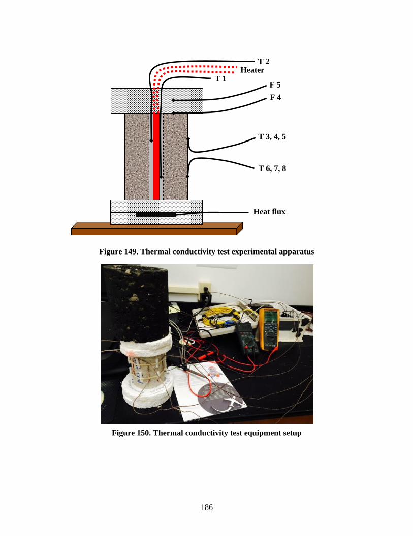
186

Figure 149. Thermal conductivity test experimental apparatus

Figure 150. Thermal conductivity test equipment setup

T 2

F 4

T 3, 4, 5

T 6, 7, 8

Heat flux

Heater

F 5 T 1

187

Testing

1. Turn on the data logger and check the measurements from all TC sensors (T1 to T8, F4 and

F5). All temperature readings should be similar. The specimen should be room temperature

at the beginning of the test.

2. Turn on the core heater with the input amperes (amps) set very low. Slowly increase the

heater input amps to reach (but not exceed) approximately 50 °C and maintain this

temperature. T1 and T2 should read a similar internal temperature, but a difference within

2 °C between T1 and T2 is acceptable.

NOTE: This test should be performed with a constant heat energy from the core heater. Use a

trial specimen to determine the target amp setting to obtain 50 °C without overheating.

NOTE: The core heater must be connected to an amp regulator to control the core heater

temperature. An amp meter and voltage meter should be connected to the electrical line to

accurately read the energy passing into the heater.

3. Record all the temperatures of T1 to T8 and calculate the K value every half hour until the

result changes less than 2%, which means the test has reached the ideal steady state. At this

point the test can be terminated.

NOTE: The test time varies due to temperature variations in the core heater, the amount of

offset of the drilled hole, and the specimen face contact material (asphalt mastic or

aggregate). Use a trial specimen to determine the probable time.

4. When the test reaches steady state, record heater amps, heater voltage, and the F4 and F5 and

T1 to T8 temperature values. Download the data logger time-series record of the test (Figure

151).

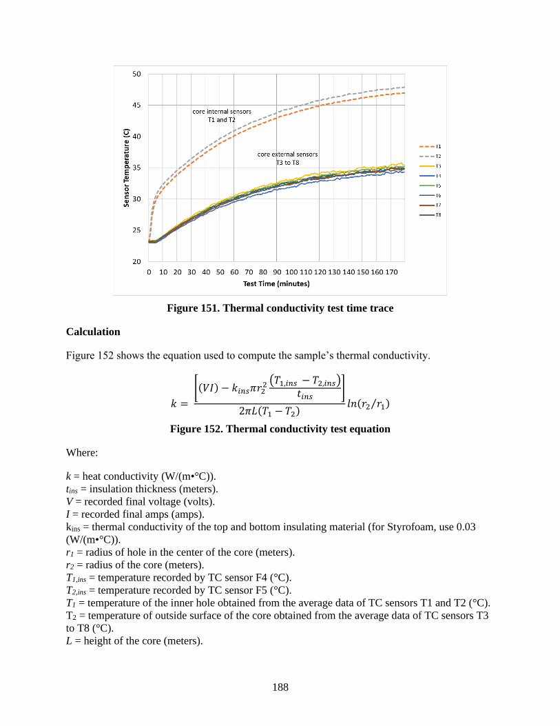
188

Figure 151. Thermal conductivity test time trace

Calculation

Figure 152 shows the equation used to compute the sample’s thermal conductivity.

𝑘 =

[(𝑉𝐼) − 𝑘𝑖𝑛𝑠𝜋𝑟22 (𝑇1,𝑖𝑛𝑠 − 𝑇2,𝑖𝑛𝑠)

𝑡𝑖𝑛𝑠]

2𝜋𝐿(𝑇1 − 𝑇2)𝑙𝑛(𝑟2 𝑟1⁄ )

Figure 152. Thermal conductivity test equation

Where:

k = heat conductivity (W/(m•°C)).

tins = insulation thickness (meters).

V = recorded final voltage (volts).

I = recorded final amps (amps).

kins = thermal conductivity of the top and bottom insulating material (for Styrofoam, use 0.03

(W/(m•°C)).

r1 = radius of hole in the center of the core (meters).

r2 = radius of the core (meters).

T1,ins = temperature recorded by TC sensor F4 (°C).

T2,ins = temperature recorded by TC sensor F5 (°C).

T1 = temperature of the inner hole obtained from the average data of TC sensors T1 and T2 (°C).

T2 = temperature of outside surface of the core obtained from the average data of TC sensors T3

to T8 (°C).

L = height of the core (meters).

189

Test Results

Taking the test results of the specimens from Texas, for example, there are five asphalt

specimens and six concrete specimens, and the test results are shown in Table 31 and Figure 153.

From Table 31, the results show the difference of mean value between the asphalt specimens and

the concrete specimens.

Table 31. Heat conductivity of Texas specimens

Specimen type Serial number

Heat conductivity

(W/(m•°C)) Mean value

Asphalt sample TX-A-1+2 1.37

1.31

Asphalt sample TX-B-1+2 1.28

Asphalt sample TX-C-1-01+03 1.26

Asphalt sample TX-C-1-02+04 1.20

Asphalt sample TX-E-01+02 1.43

Concrete sample TX-F-01-01 1.66

1.57

Concrete sample TX-F-01-02 1.37

Concrete sample TX-G-01-02 1.85

Concrete sample TX-I-01 1.59

Concrete sample TX-J-1-1 1.53

Concrete sample TX-J-1-2 1.43

Figure 153. Heat conductivity of Texas specimens

Test Limitations

• When water and sand are used to fill the inner hole, the asphalt specimens perform better

than the concrete specimens. This difference in performance is primarily a result of the

different absorptions of the materials. In the tests conducted for this study, some concrete

specimens failed to reach a uniform condition as the water was absorbed by the specimens,

which influenced the conductivity of the filler material.

190

• TC sensors T1 and T2 in the inner hole may not reach the exact same temperature at the end

of the test. This result is influenced by the performance of the core heater and the uniformity

of the water-sand filler.

• The testing time of 3 hours for this test is an improvement over earlier protocols but still

needs to be reduced for practical production testing.

HEAT CAPACITY TEST

A detailed description of the heat capacity test follows:

• Test preparation.

• Testing.

• Calculation.

• Test results.

Test Preparation

Specimen Preparation

1. Starting with 100 mm diameter drilled field cores, remove the top end of the core

(approximately 20 mm of the surface) and cut to a 125 mm length. If the core length is

insufficient to obtain a 125 mm length, then cut two cores to 62 mm lengths and bind them

together with asphalt cement. Drill a 13 mm diameter hole through the center of each core.

The 13 mm hole in the center must be carefully drilled to maintain a center location. Asphalt

specimens should be frozen prior to drilling the hole to improve drill efficiency. This reduced

temperature cools the drill bit so that the asphalt binder does not melt while the drill cuts

through the aggregate. The core must be completely air dried and brought to room

temperature before proceeding with the test. Weigh and record the dry and clean sample as

Ms, measured to the nearest 0.01 kg. (The same specimen can be used for heat capacity and

thermal conductivity tests.)

2. Prepare an approximately 60 cm length of fishing line with loops tied on both ends large

enough for fingers and strong enough to support the weight of the specimen. Place the fishing

line through the hole in the specimen. This line is used to lift and transfer the sample from

the oven to the container.

3. Place two rubber retainers around the sample to fix TC sensors F4 and F5 at the middle

height of the sample, and make sure that the tips of the TC sensors make firm contact with

the surface of the sample. Make a small hook in the tips of sensors F6 and F7 and put them

carefully into the center hole of the sample. Make sure F6 is 25 mm from the bottom of the

hole and F7 is 25 mm from the top and that the hooks make the tips of the thermocouples

touch the inner surface of the hole. Place all the four wires together, bend them to be flat at

the top of the sample, and put the assembled sample and TC sensors into the oven at a

temperature of 50 °C for at least 12 hours (see Figure 154).

191

Figure 154. Prepared specimens for heat capacity test

Water Chamber Preparation

1. Cut a 5 mm wide and 25 mm deep notch in the top of the container so that the wire leads for

TC sensors F1, F2, F3, F4, F5, F6, and F7 can be placed together and passed through the

container. Cut a similar notch in the lid and make sure to match the location of this notch to

the notch in the container. Drill a 13 mm hole in the lid at the center of the opposite half

circle that has the notch. The plastic stir will pass through this hole. Put a small porous

plastic rack (suggested dimensions of 65 mm diameter and 35 mm height) in the bottom of

the container to keep the sample off the bottom of the container and to facilitate water

circulation and thus promote the release of heat.

2. Fasten three TC sensors to a plastic rod to measure the temperature of the water at different

heights. The lowest sensor (F1) is 10 mm above the bottom of the container, the second

sensor (F2) is at the mid-depth of the water bath during the test, and the top sensor (F3) is 20

mm below the water surface during the test. Place the water bath temperature probe in the

container, arrange the three wires carefully through the notch in the container, and fix the

plastic rod along the inner side of the container. Make small bends in the tips of the three TC

sensors so the tips do not touch the container’s inner surface.

3. Make an insulating sheet (25 mm Styrofoam) that has the same diameter as the outer shell of

the container and put the sheet under the container to prevent heat loss through the bottom.

Use one or more clean plastic containers that can store water for a day of testing and keep

them at room temperature for at least 12 hours before testing. Use a trial specimen to

determine and mark the waterline in the inner surface of the container before immersing the

sample. Once the sample is placed into the water, there should be the least amount of air void

192

remaining between the top of the water and the bottom of the lid. No water should overflow

during the test (see Figure 155).

Figure 155. Inner views of heat capacity test water chamber

4. Mark the shaft of the stir rod so that when the stir paddle is in the marked position, the stir

paddle can rotate and stir the water as deep as possible without touching the sample or any

wires.

Testing

1. Weigh the mass of the storage container with water, pour the water into the test chamber to

the marked waterline, weigh the mass of the storage container with the remaining water once

again, and record the weight of the test water as Mw, which is the difference in mass of the

storage water container measured to the nearest 0.01 kg. Monitor the test water temperature

in the test chamber for 3 minutes, then measure the stable water temperature as the average

of TC sensors F1 and F2. Record the temperature as Tw measured to the nearest 0.1 °C.

2. Record the average temperature of TC sensors F4, F5, F6, and F7 as Ts to the nearest 0.1 °C

while the sample is in the oven. Quickly and carefully transfer the sample from the oven to

the container using the fishing line to minimize any heat loss during the transfer. Make sure

the sample is stable on the plastic rack base in the center of the container and that the sample

does not touch the inner surface. Then remove the fishing line from the container. Arrange

the wires of sensors F4 to F7 carefully through the notch in the test container and make sure

that the stir paddle is not influenced by the wires.

Water temp probe

Porous rack

Water level

with sample

Water fill mark

before sample

193

3. Place the lid through the hook of the stir paddle, match the container and lid notches, and

place the lid on the container. Lower the plastic stir paddle to the marked position. (The mark

should allow the pad to be as deep as possible in the water above the specimen and avoid the

TC sensors’ wire leads.) Seal the seam between the lid and the container using black

electrical tape, and turn on the stir equipment to stir the water at a speed of rotation that

creates water circulation to transfer heat from the specimen equally to the water.

4. Wrap the outside of the container with a sheet of bubble wrap and a sheet of sponge foam to

minimize any heat loss (Figure 156).

Figure 156. External insulation in the heat capacity test process

5. Record the average temperature of TC sensors F1 to F7 as Tm to the nearest 0.1 °C when the

sensors attain an equilibrium state. This takes approximately 30 minutes.

An illustration of the complete assembly is shown in Figure 157.

194

Figure 157. Heat capacity test assembly

Calculation

Figure 158 shows the equation used for the heat capacity test.

Cp,s=𝑀𝑤𝐶𝑝,𝑤∆𝑇𝑤

𝑀𝑠∆𝑇𝑠

Figure 158. Heat capacity test equation

Where:

Cp,s = specific heat capacity of the sample (kJ/(kg•°C)).

Cp,w = specific heat capacity of the water (kJ/(kg•°C), with 4.2 being typical).

Ms = mass of the sample (kg).

Mw = mass of the water (kg).

ΔTw = temperature difference of the water (=Tm-Tw, °C).

ΔTs = temperature difference of the sample (=Ts-Tm, °C).

Tw = average temperature of two sensors in the water at the beginning of the test.

Ts = average temperature of the four sensors on the core specimen in the oven at the beginning of

the test.

Tm = average temperature of all seven sensors at test equilibrium.

In this equation, heat loss through the container is neglected because it is minimal. Before the

formal test in this study, heat loss was checked using the same procedure without a specimen.

195

The water temperature uniformly dropped from 38.3 °C to 33.6 °C in 4 hours, a decrease of

2.7 °C in 4 hours. See Figure 159.

Figure 159. Heat capacity test container heat loss without specimen

The test is designed to finish within 30 minutes, so the heat loss from the container results in a

nominal 0.35 °C change in the water temperature during the testing time.

Test Results

As an example, take the results from CP Tech Sample 9. The temperature changes measured by

all seven sensors are given in Table 32, and the time-series curve is shown in Figure 160. As

Table 32 shows, TC sensors F1 and F2 in water measure the same temperature before the

beginning of the test. TC sensors F4 through F7 on the sample in the oven measure similar

temperatures, approximately 50 °C. When the specimen is transferred into the water, the

temperatures of F1 through F3 gradually rise and the temperatures of F4 through F7 begin to

drop. As the water is continually circulated by stirring, the heat gradually transfers from the

specimen to the water until 18 minutes have elapsed, at which point TC sensors F1 to F7 reach a

uniform temperature and the test is terminated.

196

Table 32. Heat capacity test numbers for CP Tech Sample 9

Time

Thermal sensor numbers (°C)

F1 F2 F3 F4 F5 F6 F7

0min 23.04 23.04 22.46 49.94 50.11 49.61 49.89

1min 23.03 23.09 22.67 43.33 44.28 42.94 43.39

2min 23.15 23.75 24.28 29.06 30.56 27.33 28.39

3min 24.96 25.39 25.17 26.29 26.72 25.32 25.88

4min 25.54 26.22 25.76 26.42 27.06 25.88 26.18

5min 25.99 26.51 26.14 26.63 27.00 26.24 26.48

6min 26.30 26.67 26.42 26.78 27.06 26.49 26.67

7min 26.51 26.78 26.59 26.89 27.06 26.66 26.83

8min 26.67 26.89 26.72 26.94 27.11 26.78 26.94

9min 26.78 26.94 26.83 27.00 27.11 26.83 26.94

10min 26.83 26.94 26.94 27.00 27.11 26.94 27.00

11min 26.94 27.00 26.94 27.00 27.11 26.94 27.06

12min 26.94 27.06 26.94 27.06 27.11 26.94 27.06

13min 27.00 27.06 27.00 27.06 27.11 27.00 27.06

14min 27.00 27.00 27.00 27.06 27.11 27.00 27.06

15min 27.00 27.00 27.00 27.06 27.11 27.00 27.06

16min 27.00 27.00 27.00 27.06 27.11 27.00 27.06

17min 27.06 27.06 27.06 27.06 27.11 27.06 27.06

18min 27.06 27.06 27.06 27.06 27.11 27.06 27.06

Figure 160. Heat capacity test time trace

197

AGGREGATE GRAYSCALE COLOR ANALYSIS

This test procedure quantifies the color of the coarse aggregate from the cut face of a pavement

core. The color is defined as the grayscale value of the aggregate surface. The grayscale values

are quantified on a grayscale standard sheet developed for this test.

Preparation for the Procedure

Specimen Preparation

Obtain the pavement core from the field and thoroughly wash it to remove any cutting-related

dust generated by the coring operation. Allow the core to air dry.

Digital Image Station Preparation

Set up a digital camera on a tripod. The background for the digital images should be a neutral,

non-glossy surface. The field of view needs to capture the cut surface of the core and the entire

grayscale standard sheet. Lighting for the image should be from external sources and should be

arranged to avoid any glare from the core or grayscale sheet. Do not use the camera’s flash

because the flash may also cause glare. Mark the corners of the field of view on the background

surface so it is easy to lay out the core and grayscale sheet.

Grayscale Standard Sheet

The grayscale standard sheet can be prepared from a simple Microsoft Word file. Insert a two-

column, five-row table into a blank page. Fill the cells with a progression of gray tones using

preset fill colors. Use the “Custom Colors” feature to match each cell’s gray tone to the red-

green-blue (RGB) value listed. White has a RGB value of 255, and black has a RGB value of 0.

Type the corresponding RGB value into the cell. These RGB values are the grayscale values

used to quantify the aggregate’s color. An example of a grayscale standard sheet created in

Microsoft Word is shown in Table 33.

Table 33. Sample grayscale standard sheet

255 25

224 50

199 75

174 100

150 125

198

The grayscale standard sheet shown in the digital image with the core must be an original sheet

printed on a high-quality printer.

Steps to Determine Aggregate Grayscale Value

1. Place the core on its side on top of the image station background.

2. Place a sample identification card above or next to the core in the camera’s field of view.

3. Place the grayscale standard sheet on top of a small box so that the height of the grayscale

sheet aligns to the height of the core. The height of the core and grayscale sheet will be 100

mm in most cases.

4. With the image station lighting on, take a digital image of the core and grayscale sheet side

by side (see Figure 161).

Figure 161. Grayscale analysis image station setup

5. Review the digital image to confirm that the image is in focus and that no areas show glare

from the lighting.

6. Save the color JPEG image.

7. Open the JPEG image for editing with Microsoft Photos.

8. Select the “Edit” feature, then select the “Color” icon.

9. Reduce the color saturation to the lowest setting. This converts the image to black and white.

10. Save the black and white JPEG image with a new file name.

199

11. Open the black and white JPEG image with Microsoft Paint.

12. Using the area select feature, highlight an exposed coarse aggregate. The aggregate must be

from the mixture exposed on the surface of the pavement.

13. Drag the highlighted image to the grayscale sheet and match the image color to the closest

grayscale cell. Leave the image in the cell.

14. Repeat the highlight-and-match process for three to five exposed coarse aggregates. If the

core has coarse aggregate from two distinctly different sources (and of different colors),

match at least three exposed surfaces for each source.

15. Compute the coarse aggregate color as the average of the grayscale values matching the

exposed coarse aggregate images. In the image in Figure 161, the computed coarse aggregate

color is (174+150+125+125+125)÷5=138. If two sources with different colors are observed,

compute a weighted average based on the percent of exposure for each source.

16. Save the JPEG file as a record of the grayscale color test.

NOTE: It is not recommended to photograph the cores alone without the accompanying

grayscale chart and then edit these digital images directly using photo editing software. The

grayscale values measured by the photo editing software are significantly influenced by the

lighting in the original digital image. A bright image will exhibit higher grayscale values, and a

dark image (of the same material) will exhibit lower grayscale values. Photographing the core

with the grayscale standard sheet in the view creates a digital image with both the core and the

grayscale sheet in the same degree of light.

201

APPENDIX B: PAVEMENT THERMAL MODEL USER GUIDE

The following guide provides a detailed explanation of the operation of the spreadsheet-based

pavement thermal model created for this project. This spreadsheet is available as part of the file

available at https://cptechcenter.org/research/completed/quantifying-pavement-albedo/ and

contains the following elements:

• Sheet #1 is “Graphs,” which contains a set of thermal and physical parameters for each of the

involved pavement, base, and subbase materials. These parameters include specific heat,

thermal conductivity, emissivity, and density.

• Sheet #2 is “Data,” which contains a set of necessary thermal modeling coefficients and

constants for the involved convective, radiative, and conductive heat transfer equations, as

well as a similar set of values for dew point determinations.

• Sheet #3 is “PCCdry,” in which the actual material temperatures are determined. All weather,

ambient environmental, and albedo data are loaded into this sheet in sequential time-of-day

order (by row), and all subsequent calculations of pavement, base, and subbase temperatures

are based on a heat energy mass-balance determination around each subsurface cell.

This model has two levels of high resolution, both in regards to time (most runs were completed

at one-minute intervals) and iterative depths (i.e., increments were measured at the centimeter

level). Depth variations in the pavement layer were kept at 1 to 2 cm due to the high levels of

heat energy at this upper level. Depth variations in the base were similarly held to about 2 cm.

However, subbase depths varied from a few centimeters (just below the base level) to

approximately 20 cm at the lower subbase depth, given the far lower rate of flux of heat energy

transfer at this lower, more thermally stable depth.

This summary uses five sequential steps to explain the operation of this model. Due to the nature

of this model and its high levels of temporal (minute by minute) and physical (centimeter-level)

resolution, this Excel spreadsheet is large and time consuming to operate. One precautionary

recommendation is to switch the model’s formula mode from “automatic” to “manual” when

making any changes to the data or the modeling equations so that the model remains static and

stable until a decision is made to switch back to the “automatic” formula mode, which then

reactivates the entire model.


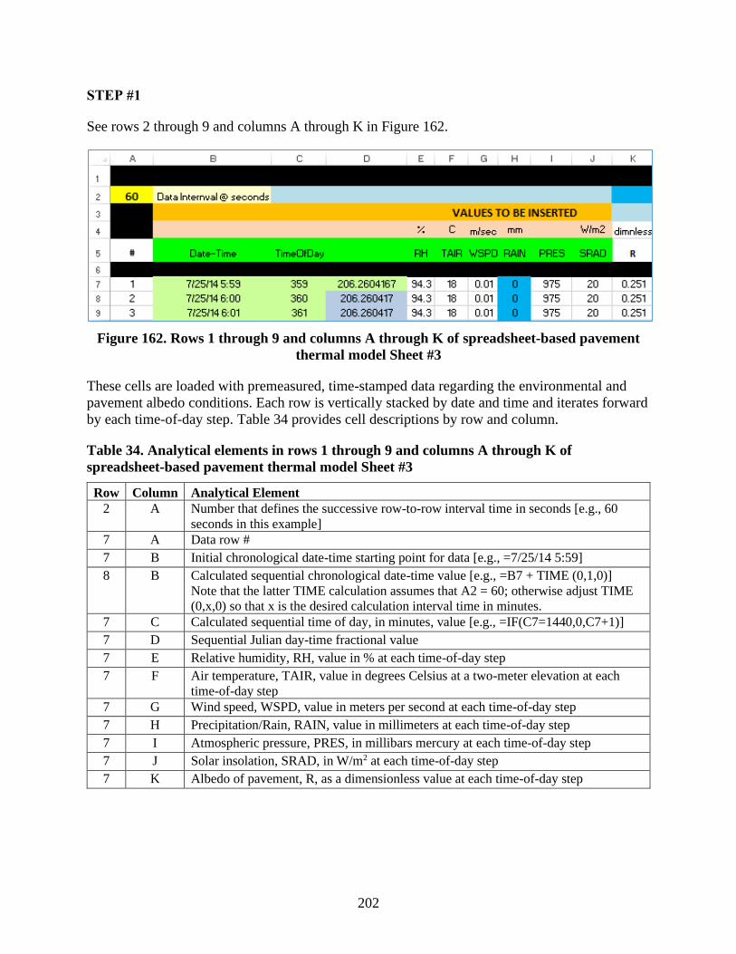
202

STEP #1

See rows 2 through 9 and columns A through K in Figure 162.

Figure 162. Rows 1 through 9 and columns A through K of spreadsheet-based pavement

thermal model Sheet #3

These cells are loaded with premeasured, time-stamped data regarding the environmental and

pavement albedo conditions. Each row is vertically stacked by date and time and iterates forward

by each time-of-day step. Table 34 provides cell descriptions by row and column.

Table 34. Analytical elements in rows 1 through 9 and columns A through K of

spreadsheet-based pavement thermal model Sheet #3

Row Column Analytical Element

2 A Number that defines the successive row-to-row interval time in seconds [e.g., 60

seconds in this example]

7 A Data row #

7 B Initial chronological date-time starting point for data [e.g., =7/25/14 5:59]

8 B Calculated sequential chronological date-time value [e.g., =B7 + TIME (0,1,0)]

Note that the latter TIME calculation assumes that A2 = 60; otherwise adjust TIME

(0,x,0) so that x is the desired calculation interval time in minutes.

7 C Calculated sequential time of day, in minutes, value [e.g., =IF(C7=1440,0,C7+1)]

7 D Sequential Julian day-time fractional value

7 E Relative humidity, RH, value in % at each time-of-day step

7 F Air temperature, TAIR, value in degrees Celsius at a two-meter elevation at each

time-of-day step

7 G Wind speed, WSPD, value in meters per second at each time-of-day step

7 H Precipitation/Rain, RAIN, value in millimeters at each time-of-day step

7 I Atmospheric pressure, PRES, in millibars mercury at each time-of-day step

7 J Solar insolation, SRAD, in W/m2 at each time-of-day step

7 K Albedo of pavement, R, as a dimensionless value at each time-of-day step

203

STEP #2

See rows 1 through 9 and columns L through S in Figure 163.

Figure 163. Rows 1 through 9 and columns L through S of spreadsheet-based pavement


These cells are used to calculate a collection of necessary parameters and coefficients for the

thermal model calculations. The rows iterate forward by each time-of-day step. Table 35

provides cell descriptions by row and column.

204

Table 35. Analytical elements in rows 1 through 9 and columns L through S of spreadsheet-

based pavement thermal model Sheet #3


7 L Calculated air temperature, TAIR, value in kelvins at each time-of-day step [e.g.,

=F8+273.15]

7 M Calculated sky temperature, Tsky, value in kelvins at each time-of-day step [e.g.,

=L7×(0.8+0.004×O7)^0.25)]

7 N Calculated Magnus coefficient, m, as a dimensionless value at each time-of-day

step

[e.g., =

LN(E7÷100)×EXP(Data!$I$40−F7÷Data!$I$42)×(F7÷(Data!$I$41+F7))))] where

Data!$I$40 = 18.678, Data!$I$41 = 257.14 & Data!$I$42 = 234.5

7 O Calculated dew point temperature, Tdew, value in kelvins at each time-of-day step

(i.e., as per the Magnus formula)

[e.g., =(Data!$I$41×N7)÷(Data!$I$40−N7)] where Data!$I$41 = 257.14 and

Data!$I$40 = 18.678

7 P Calculated average of the surface temperature (column AC) and the air

temperature at a two-meter height (column F) above the pavement, Tm, value in

kelvins at each time-of-day step [e.g., =(AC6+F7)÷2]

7 Q Calculated initial convective heat transfer per unit area from the surface to the air,

h1, value in watts per square meters at each time-of-day step

[e.g., =0.00144×(P7+273.15)^(0.3)×(G7)^(0.7)]

7 R Calculated secondary convective heat transfer per unit area from the surface to the

air, h2, value in watts per square meters at each time-of-day step

[e.g., =IF(AC6>F7,0.00097×(AC6-F7)^(0.3),0)]

7 S Calculated net convective heat transfer per unit area from the surface to the air,

hnet, value in watts per square meters at each time-of-day step

[e.g., =698.2×(Q7+R7)]

STEP #3

See rows 1 through 9 and columns T through AB in Figure 164.

Figure 164. Rows 1 through 9 and columns T through AB of spreadsheet-based pavement


These cells are used to determine the actual thermal heat transfer calculations. Each row is

vertically stacked by date and time and iterates forward by each time-of-day step. Table 36

provides cell descriptions by row and column.

205

Table 36. Analytical elements in rows 1 through 9 and columns T through AB of



7 T Calculated absorbed heat flow rate, qabs, value in joules per time interval (e.g., 60

seconds) at each time-of-day step [e.g., =$A$2×(1-K8)×J8] where $A$2 = data

time interval

7 U Calculated radiative heat flow rate, qrad, value in joules per time interval (e.g., 60

seconds) at each time-of-day step [e.g., =$A$2×5.67×POWER(10,-

8)×Graphs!$C$5×(AC7+273.15)^4−(M8)^4) where $A$2 = data time interval;

and Graphs!$C$5 = emissivity, E, of pavement surface (e.g., 0.93)]

7 V Calculated cumulative net radiative heat flow, qRad_net, value in joules at each

time-of-day step [e.g., =V7+$U8].

Note that these values are only determined for tracking purposes.

7 W Calculated convection heat flow rate, qconv, value in joules per time interval

(e.g., 60 seconds) at each time-of-day [e.g., = $A$2×S8×(AC7−F8)] where $A$2

= data time interval

7 X Calculated cumulative net convective heat flow, qConv_net, value in joules at

each time-of-day step [e.g., =X7+$W8].


7 Y Calculated cumulative net conductive heat flow rate at the top of the pavement

surface, qCond_TOP, value in joules per time interval (e.g., 60 seconds) at each

time-of-day step

[e.g., =$A$2×AD$3×1×(AC7+273.15)-(AD7+273.15))÷(AD$1−AC$1)÷100)]

where $A$2 = data time interval


7 Z Calculated cumulative net conductive heat flow rate within the pavement depth,

qCond_HF, value in joules per second per square meter, or W/m2-sec, at each

time-of-day step; note also that this qCond-HF value represents the heat flux (HF)

[e.g., =Y8÷$A$2] where $A$2 = data time interval


7 AA Calculated cumulative heat flux at the top of the pavement surface, flux_TOP,

value in joules per time interval (e.g., 60 seconds) at each time-of-day step

[e.g., =SUM(T8−U8−W8−Y8)]


7 AB Calculated cumulative temperature change at the top of the pavement surface,

temp_TOP, value in kelvins at each time-of-day step

[e.g., =(AA8÷1000)÷(AD$2×AD$4×10×(AD$1-AC$1)÷2))]


206

STEP #4

See rows 1 through 9 and columns AB through AS in Figure 165.

Figure 165. Rows 1 through 9 and columns AC through AS of spreadsheet-based pavement


These cells are used to determine the actual pavement, base, and subbase temperatures at each

specific depth level (sequential column). The rows iterate forward by each time-of-day step to

produce sequential rows. Table 37 provides cell descriptions by row and column.

Table 37. Analytical elements in rows 1 through 9 and columns AC through AS of



1 AC-AS Vertical depth [AC = 0 @ surface, AB = 1.6 cm, AC = 2.8 cm, etc.]

2 AC-AS Specific heat values of pavement, base, or subbase material at each specific depth

level

3 AC-AS Specific thermal conductivity values of pavement, base, or subbase material at each

specific depth level

4 AC-AS Density values of pavement, base, or subbase material at each specific depth level

5 AC-AS Depth profile tracking number [e.g., AD5 = 1] as the position below the pavement

surface

6 AC-AS Initial estimate values for pavement, base, and subbase temperatures at each iterative

vertical depth at time = 0 model time, in degrees Celsius

7 AC-AS Calculated values for the pavement surface temperature at each sequential time-of-day

step, in degrees Celsius [e.g., =(AC6+273.15)+AB7)−273.15]

7 AC-AS Calculated values for pavement, base, or subbase temperatures at each iterative

vertical depth at each sequential time-of-day step, in degrees Celsius [e.g.,

=(AD$3×1×(AC6−AD6)÷(AD$1−AC$1)÷100)+AE$3×1×(AE6−AD6)÷(AE$1−AD$

1)÷100))×60÷(1000×(AD$4×1000×AD$2×(AD$1−AC$1)÷200)+AE$4×1000×AE$2

×(AE$1−AD$1)÷200)))+AD6]

207

STEP #5

See rows 1 through 9 and columns CP through DB in Figure 166.

Figure 166. Rows 1 through 9 and columns CP through DB of spreadsheet-based pavement


These cells are again used to determine the actual material temperatures at each specific depth

level (i.e., each sequential column). The rows iterate forward by each time-of-day step to

produce sequential rows. Note that by this set of columns (e.g., CP through DB), the vertical

depth has dropped well into the subbase material depth. It should also be noted that columns AS

through CO are not shown because their mode of operation is much the same, albeit for what

may be pavement, base, or subbase materials with different thermal properties. Table 38 provides

cell descriptions by row and column.

Table 38. Analytical elements in rows 1 through 9 and columns CP through DB of


Row Column Analytical Elements

1 CP- DA Cumulative vertical depth, in centimeters

2 CP- DA Specific heat values of subbase material at each specific depth level, in centimeters, in

kilojoules per kilogram per kelvin

3 CP- DA Specific thermal conductivity values of subbase material at each specific depth level, in

watts per meter per kelvin

4 CP- DA Density values of subbase material at each specific depth level, in grams per cubic

centimeter

5 CP- DA Depth profile tracking number

6 CP- DA Initial estimate values for subbase temperatures at each iterative vertical depth at time

= 0 model time, in degrees Celsius

7 CP- DA Calculated values for the subbase material temperature at each sequential time-of-day

step, in degrees Celsius [e.g.,

=(DA$3×1×(CZ6−DA6)÷(DA$1−CZ$1)÷100)+DB$3×1×(DB6−DA6)÷(DB$1−DA$1)

÷100))×60÷(1000×(DA$4×1000×DA$2×(DA$1-

CZ$1)÷200)+DB$4×1000×DB$2×(DB$1−DA$1)÷200)))+DA6]

Quantifying Pavement Albedo Final Report

Documents

Transcript of Quantifying Pavement Albedo Final Report