COOPERATIVE RESEARCH CENTRE FOR COAL IN SUSTAINABLE DEVELOPMENT Established and supported under the Australian Government’s Cooperative Research Centres Program

QUANTIFYING NATURAL AND ANTHROPOGENIC SOURCED

MERCURY EMISSIONS FROM AUSTRALIA IN 2001

-A local scale modelling assessment of transport and deposition patterns for anthropogenic mercury air emissions

RESEARCH REPORT 46

Authors:

Christian Peterson Peter Nelson

Anthony Morrison

Macquarie University

April 2004 QCAT Technology Transfer Centre, Technology Court

Pullenvale Qld 4069 AUSTRALIA Telephone (07) 3871 4400 Facsimile (07) 3871 4444

Email: Administration@ccsd.biz

This page is intentionally left blank

DISTRIBUTION LIST CCSD Chairman; Chief Executive Officer; Research Manager, Manager Technology; Files Industry Participants Australian Coal Research Limited ............................................................. Mr Ross McKinnon BHP Billiton Minerals - Coal .................................................................... Mr Ross Willims ................................................................................................................ Mr Alan Davies CNA Resources.......................................................................................... Mr Ashley Conroy CS Energy .................................................................................................. Dr Chris Spero Delta Electricity ......................................................................................... Mr Steve Saladine Queensland Natural Resources, Mines and Energy................................... Mr Bob Potter Rio Tinto (TRPL)....................................................................................... Mr David Cain .................................................................................................................... Dr Jon Davis Stanwell Corporation ................................................................................. Dr Paul Simshauser Tarong Energy ........................................................................................... Mr Burt Beasley The Griffin Coal Mining Co Pty Ltd ......................................................... Mr Jim Coleman Wesfarmers Premier Coal Ltd ................................................................... Mr Peter Ashton Western Power ........................................................................................... Mr Keith Kirby Xstrata Coal Australia Pty Ltd................................................................... Mr Barry Isherwood Research Participants CSIRO ……............................................................................................... Dr David Brockway Curtin University of Technology ............................................................... Dr Barney Glover Macquarie University ................................................................................ Prof Jim Piper The University of Newcastle ..................................................................... Prof Adrian Page The University of New South Wales ......................................................... Prof David Young The University of Queensland ................................................................... Prof Don McKee

This page is intentionally left blank

Cooperative Research Centre for Coal in Sustainable Development

QCAT Technology Transfer Centre Technology Court

Pullenvale, Qld 4069 Telephone: (07) 3871 4400

Fax: (07) 3871 4444

Feedback Form To help us improve our service to you may I ask you for five minutes of your time to complete this

questionnaire. Please fax or mail it back to me, or, if you would prefer, give me a call.

ATTENTION MANAGER TECHNOLOGY TRANSFER FAX NO 07 3871 4444 DATE ............................................................................... FROM NAME: .................................................................................................................................. COMPANY:............................................................................................................................ REPORT TITLE: QUANTIFYING NATURAL AND ANTHROPOGENIC SOURCED MERCURY EMISSIONS FROM

AUSTRALIA IN 2001 AUTHORS: CHRISTIAN PETERSON, PETER NELSON, ANTHONY MORRISON Would you please rate our performance in the following areas by ticking the appropriate box:

The Research Agree Neutral Disagree Don’t Know

This work has achieved its research objectives

This work has delivered to agreed milestones

This work is relevant to my organisation

Communication of progress has been timely & useful

The Report

The report is well presented

The context of the report is clear

The content of the report is substantial

The report is clearly written and understandable

This product is good value

Any further comments which would assist us in better serving your future requirements?: …………………………….……………………………………………………………………………………………

…………………………………………………………………………….……………………………………………

Are there any people you would like to add to our distribution list?:

………………………………………………………………………………………………………….………………

………………………………………………………………………………………………………………….…....... Thank you for your response

This page is intentionally left blank

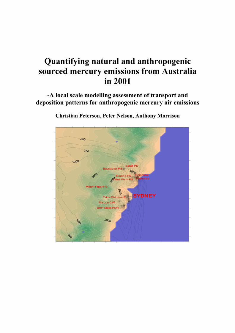
Quantifying natural and anthropogenic sourced mercury emissions from Australia

in 2001

-A local scale modelling assessment of transport and deposition patterns for anthropogenic mercury air emissions

Christian Peterson, Peter Nelson, Anthony Morrison

Mount Piper PS

Maldon CW

BHP Steel PKW

Orica Chlorine P SYDNEY

Vales Point PSEraring PS

PasmincoComsteel

Lidell PSBayswater PS

i

SUMMARY Mercury is continuously released both directly and indirectly to the atmosphere from anthropogenic and natural sources (i.e. oceans, land and vegetation) by emission and re-emission. The atmosphere also constantly deposits mercury by a variety of mechanisms to receiving natural surfaces. Thus, mercury is continually cycled between the air and the natural environment until it is finally stored in soil and sediments (or alternatively converted to methyl-Hg). Elevated levels of mercury are today found in sediment and fish tissue around the world. Although mercury is naturally occurring, the total amount of mercury in the environment has increased by a factor of two to five compared to pre industrial levels. Due to its global mobility it is suggested that a significant proportion of the children born each year are at risk of adverse neurological effects caused by mercury.As the pre-eminent source of anthropogenic mercury is fuel combustion, particularly coal, there is a need to understand its role as a mercury source. A number of studies have estimated that the yearly total global input of mercury to the atmosphere ranges between 5800-7000 tonnes. Of these emissions, somewhere between 35-60 % originates from anthropogenic sources. However, if re-emission of anthropogenic mercury previously deposited on natural surfaces is taken into account, the anthropogenic portion of the total global mercury emissions may be as high as 75 percent. Calculations performed as part of this study have estimated that mercury emissions from natural sources in Australia are in the range 130-270 tonnes/yr. However, these estimates were based on a number of simplifying assumptions and the result should be treated with some caution. Because of its physio-chemical properties mercury is used in a broad variety of manufacturing industries and products, although this use is diminishing. The processing of mineral resources at high temperatures such as roasting and smelting of ores, combustion of fossil fuels, kiln operation in the cement industry, and waste incineration all release significant amounts of mercury to the atmosphere. Global anthropogenic sources are estimated to have emitted 1900 tonnes of mercury in 1995. The most significant source of global anthropogenic mercury is the stationary combustion of fossil fuels (mainly coal), which accounts for 77 percent of total emissions. Of the approximately 10.2 tonnes of anthropogenic Hg released annually in Australia, it is estimated that about 9.9 tonnes is emitted into the atmosphere, with the remaining 0.3 tonnes distributed between the water and land compartments. Of the mercury emitted into the atmosphere it was calculated that 4.75 tonnes (48 %) are in the form of elemental mercury (Hg0), 1.30 tonnes is in the form of divalent mercury (13 %), and 3.88 tonnes (39 %) is particulate mercury. This elemental mercury becomes part of the global atmospheric mercury pool, and the Australian contribution constitutes about 0.5 percent of the annual increase in the global mercury pool. Even though the estimated emissions from Australia are only minor, because of a dependence on a resource based economy, the country is a significant per capita emitter (0.51 g Hgtot/person), compared to the global average (0.36 Hgtot/person). It is apparent that mercury emission inventories are subjected to large uncertainties. According to the latest global emission inventory, Australia was claimed to annually emit more than 110.9 tonnes of anthropogenic mercury. This value is nearly 11 times more than that estimated by the Australian National Pollution Inventory. The report demonstrates that the former value of 110.9 tonnes is unrealistically high and that the discrepancy between the calculated values is predominantly due to the use of inappropriate emission factors when calculating the mercury emitted from the combustion of coal. The dispersion and deposition of mercury from ten significant industrial point source emitters in the central, coastal parts of NSW was investigated using a three-dimensional, regional

ii

scale, Eulerian air quality model (TAPM). Since the model was primarily developed to investigate the air quality of an airshed in relation to SOx, NOx, and photochemical smog, mercury was modelled as an inert pollutant (tracer) where chemical transformation processes, as well as, wet deposition processes are omitted For simplicity a facility emission cutoff of 20 kg/yr was used which ensured that more than 90 % (1282 kg/yr) of the total anthropogenic point emissions in NSW (NPI, 2003a) were embraced by the simulation. The sources of Hg emissions simulated include: combustion of coal (5 power plants), basic iron and steel manufacturing (2 sources), cement manufacturing (1 source), Cu/Ag/Pb/Zn smelter (1 source), and chemical production (1 source). A simulation was conducted for the January 2001 period. The model used 25×25 grids in the outer domain with a grid size of 30×30 km. In order to obtain a finer resolution for concentration simulations, an outer and an inner pollution grid domain was used with 97×97 grids in the horizontal plane, with grid sizes of 7.5 × 7.5 km and 2.5 × 2.5 km. Vertically, there were 25 non-uniform layers in the model, with the finest resolution near the surface (10 m). The top of the modeling domain was 8 km. The mercury species considered in the simulation were Hg0 and Hg(II)/Hgp (combined) and the background concentration of Hg0 was set to zero. Even though deposition of mercury was not included in TAPM, dry deposition fluxes were calculated by post-processing hourly-simulated grid concentration outputs from TAPM. Hourly dry deposition fluxes were derived from each grid cell using default values for the deposition velocities. The deposition velocity for Hg(II)/Hgp was set to be 0.5 cm/s during the day and zero cm/s during the night, corresponding values for Hg0 were respectively, 0.03 and zero cm/s. The simulation calculated that the maximum ambient ground level mercury concentration was 3.1 ng/m3. Even if the background concentration of Hg0 is added to this value the total was well below (i) the US EPA determined reference concentration of Hg vapor of 0.3 µg/m3 for the general population, (ii) the limit value for exposure in Europe of 0.05µg/m3, and (iii) the air quality objectives set in Victoria, Australia, of 9.4 µg/m3, for inorganic mercury,. The simulated total average mercury deposition flux in the inner domain varied between 0.2 and 1.4 µg/m2/yr (at the 10th and 90th percentile level, respectively). In occasional cases, close to emitting sources (1-2 grid cells away from the source), the deposition flux of Hgtot was calculated to reach levels of 50-60 µg/m2/yr. A number of further calculations were performed to investigate the area average deposition flux of mercury and the percentage of total mercury deposited at various distances from the emitting sources. The general trend observed from these calculations was that the area average deposition flux of mercury, when expressed as a percentage of the total mercury emitted, is relatively small, (0.1-9.4 %, depending on the distance to the source). Thus it appears that, a significant part of the mercury emitted from the facilities investigated would be transported away from the domain. By integrating the average simulated deposition rate in the outer domain over the area of study, it was calculated that approximately 105 kg of mercury would be deposited annually within the entire domain. This constitutes about 8 % of the total mercury emissions in the simulation. The numerous mercury species present in the atmosphere have differing atmospheric residence times, which affect the distance they can be transported before being deposited to the surface. Atmospheric transformation/interaction processes, which determine the speciation of mercury, are therefore important to include if models are to accurately simulate mercury transportation and deposition. In order to obtain more accurate data in future simulations, mercury transformation/interaction and deposition processes should be integrated into the TAPM model.

iii

The study has allowed the establishment of an initial methodological framework for assessing the environmental impact of mercury (and in the future other trace elements) from power stations and other major emission sources.

iv

TABLE OF CONTENTS

Page

ABSTRACT i

TABLE OF CONTENTS iii

LIST OF TABLES vi

LIST OF FIGURES viii

1. INTRODUCTION 1

1.1 Background 1

1.2 The purpose and scope of this report 5

2. ATMOSPHERIC CHEMISTRY AND RESIDENCE TIME 6

2.1 The properties of atmospheric mercury species 6

2.2 Chemical reaction and interaction in the atmosphere 9

3. EMISSION OF MERCURY 12

3.1 Definition 12

3.2 The global atmospheric Hg cycle 12

3.3 Natural mercury emission 16

3.3.1 Background 16

3.3.2 Bi-directional exchange of mercury 17

3.3.3 Estimated natural emissions of mercury from Australia 21

3.4 Anthropogenic mercury emissions 25

3.4.1 Global anthropogenic emissions 26

3.4.2 2001 Australian mercury emission inventory 32

3.4.2.1 Atmospheric emission from point sources 32

3.4.2.2 Atmospheric emission from area sources 34

3.4.2.3 Total Australian anthropogenic emission 35

3.4.2.4 Accuracy of emission estimates 35

3.4.2.5 Estimation of mercury speciation 40

v

TABLE OF CONTENTS (cont)

Page

4. DEPOSITION OF MERCURY 43

4.1 Dry deposition 44

4.2 Deposition patterns of mercury 46

4.3 Model simulation 48

4.3.1 The Model 48

4.3.2 Simulation procedure 48

4.3.2.1 Simulation domain and period 48

4.3.2.2 Meteorological conditions 50

4.3.2.4 Mercury emission data 50

4.3.2.4 Initial and boundary conditions 50

4.3.2.5 Deposition 50

4.3.3 Simulation result 51

4.3.3.1 The simulation 51

4.3.3.2 Ambient mercury concentrations 51

4.3.3.3 Dry deposition of mercury 53

5. THE CHEMISTRY OF ATMOSPHERIC MERCURY 61

5.1 Chemical transformations in the aqueous phase 63

5.1.1 Oxidation 63

5.1.1.1 Oxidation of Hg0 by O3 63

5.1.1.2 Oxidation of Hg0 by ·OH 64

5.1.1.3 Oxidation of Hg0 by chlorine (HOCL/OCL-) 65

5.1.2 Reduction 67

5.1.2.1 Reduction of Hg(ΙΙ) by S(ΙV) 67

5.1.2.2 Photoreduction of Hg(ΙΙ) 69

5.1.2.3 Reduction of Hg(ΙΙ) by HO2 69

5.2 Chemical transformations in the gaseous phase 70

5.2.1 Oxidation of Hg0 by O3 70

5.2.2 Oxidation of Hg0 by ·OH 71

5.2.3 Oxidation of Hg0 by NO3· 72

TABLE OF CONTENTS (cont)

vi

Page 5.2.4 Oxidation of Hg0 by H2O2

72

5.2.5 Dimethyl mercury reactions 73

5.2.5.1 Reaction with nitrate radical 73

5.2.5.2 Reaction with other species 74

5.3 Equilibria tables 75

5.4 Summary of half lives and residence times for elemental and

divalent mercury 76

6. CONCLUSIONS 77

7. ACKNOWLEDGEMENTS 79

8. REFERENCES 80

APPENDIX A Estimated Hg emissions by point source in Australia 2001 A1

APPENDIX B Estimation of Hg emission from area sources related to

the Pacyna and Pacyna (2002) study B1

APPENDIX C Input data to TAPM C1

APPENDIX D Simulation result from TAPM D1

CONTACT DETAILS

vii

LIST OF TABLES

Page

Table 1 Post and pre-industrial mercury fluxes recorded in lake sediment cores 3

Table 2 Chemical transformations in the aqueous phase 10

Table 3 Chemical transformations in the gaseous phase 11

Table 4 Estimated global emissions (tonnes/yr) (Mason et al., 1994) 14

Table 5 Estimated global emissions (tonnes/yr) (Bergan and Rohde, 2001) 15

Table 6 Summary of estimated global emissions (tonnes/yr) 16

Table 7 Emission rates of mercury from different natural surfaces 19

Table 8 Global natural emission of mercury from forests (Lindberg et al., 1998) 20

Table 9 Estimated emission of mercury from natural land surfaces in Australia 24

Table 10 Global atmospheric emissions of total mercury from major anthropogenic

sources in 1995 (tonnes) 26

Table 11 Estimated 1995 mercury emissions from area and point sources

in various countries (tonnes) 29

Table 12 Distribution of total estimated Australian anthropogenic mercury (kg)

for 2001 35

Table 13 Country-by-country comparison based on anthropogenic atmospheric

Hgtot/capita 39

Table 14 Emission speciation (fraction of the total) of mercury from anthropogenic

sources 41

Table 15 Estimates of Australian atmospheric mercury emission rates by source (2001) 42

Table 16 Dry deposition velocity of mercury species (cm/s) 46

Table 17 Percentile analysis of simulated ambient mercury concentration 52

Table 18 Percentile analysis of simulated dry deposition fluxes of mercury species 53

Table 19 Area average mercury deposition rates around each facility (Run 10) 58

Table 20 Percent of total mercury dry deposited around each facility (Run 10) 58

Table 21 Area average mercury deposition rates around each facility (Run 20) 59

Table 22 Area average mercury deposition rates around each facility (Run 30) 59

Table 23 Percent of total mercury dry deposited around each facility (Run 20) 60

Table 24 Percent of total mercury dry deposited around each facility (Run 30) 60

Table 25 Oxidation of DMM with different oxidants 74

viii

LIST OF TABLES (continued)

Page

Table 26 Equilibria for aqueous phase Hg(II) speciation 75

Table 27 Solid-liquid equlibria of mercury compounds 75

Table 28 Gas/aqueous equlibria of Hg and some of its compounds 75

Table 29 Summary chemical transformations in the aqueous phase 76

Table 30 Summary chemical transformations in the gaseous phase 76

ix

LIST OF FIGURES

Page

Figure 1 Mercury oxidation, reduction and mass transfer processes in the atmosphere 8 Figure 2 The global atmospheric mercury cycle 13 Figure 3 Geographical distribution of mercury emissions over Australia and South-East Asia (tonnes/yr) 28 Figure 4 Estimated mercury emissions (point sources) from Australian States and Territories (2001) (kg/yr) 33 Figure 5 Estimated mercury to air (point sources) by source category in Australia, 2001 (kg/yr) 33 Figure 6 Geographical distribution of mercury emitting point sources in Australia 34 Figure 7 Estimates made using NPI (1999b, 2003b) emission factors of Australian anthropogenic atmospheric mercury emissions from fuel and coal combustion compared with emissions which arise from combustion during electricity generation 37 Figure 8 Geographical distribution of point sources include in the TAPM simulation 49 Figure 9 Contour plot of simulates of dry deposition of divalent /particulate Hg (unit: µg/m3) 55 Figure 10 Contour plot of simulates of dry deposition of elemental Hg(unit: µg/m3) 56 Figure 11 The magnitude of dry deposition fluxes from TAPM simulation(unit: µg/m3) 57 Figure 12 Atmospheric mercury chemistry 61

1

1. INTRODUCTION

1.1 Background

Mercury (Hg) is among the most bio-concentrated trace metal in the food chain, especially in

fish tissue. Consumption of fish with elevated concentrations of Hg may lead to adverse

health affects and can in some cases even be lethal. There are several historical examples of

severe poisoning disasters. For instance, in Minimata Bay (Japan), in the 1950s, a large

number of people were severely poisoned by eating fish (their primary source of food)

polluted with Hg (methyl mercury) by local industries. Methyl mercury was accumulated in

marine organisms in the bay over time until the level of concentration in fish tissue exceeded

a healthy dose. Many people died and others were faced with a variety of neurological

problems. In particular, children, who had been exposed to Hg in the womb, suffered serious

developmental deficits (Goldfrank et al,. 1990). This is a somewhat unusual and extreme

example, however, elevated levels of Hg are today found in sediment and fish tissue around

the world. Even if the concentration is modest, long-term "exposure" can present a significant

risk to humans and wildlife. Accumulated levels of Hg in the human body can cause, as

mentioned in the example above, developmental distortion in features, as well as permanent

damage to the kidneys and the central nervous system (WHO, 1990 and 1991). According to

the US Centre for Disease Control and Prevention, 10 percent of American women already

have so much Hg in their blood that if they become pregnant, it would pose a threat to the

developing fetus (US CDC, 2001). It has been estimated that at least 60 000 children born

each year in the US are at risk of adverse neurological effects from Hg (US NAS, 2000).

Since the Hg exposure pathway of the greatest concern is consumption of fish contaminated

with methyl mercury (US EPA, 1997)1, many countries have issued fish consumption

advisories for waterbodies with elevated levels of methyl mercury, as well as, introduced

information campaigns addressed to women which aim to increase awareness about the risks

of eating fish during their pregnancy (Schroeder and Munthe, 1998). Although Hg is naturally

occurring, the total amount of Hg in the environment has increased by a factor of two to five

compared to pre-industrial levels (Mason et al., 1994). As the amount of Hg is increasing in

the environment so is the risk of exposure to methyl mercury (US EPA, 1997).

1 Vaporised elemental mercury is also of concern when inhaled. Even at low levels, mercury can cause permanent damage to the brain and central nervous system (EPA, 2000). However, ambient air concentrations of elemental Hg are approximately in the range of 2 - 10 ngm-3. Compared to the US EPA reference concentration for elemental Hg of 0.3 µgm-3 for the general population, ambient air exposure of elemental Hg are unlikely to pose a significant risk to human health (US EPA, 1997). In Europe, the annual average limit of Hg exposure is 0.05 µgm-3 (Pirrone et al., 2001b).

2

Due to the seriousness of the health effects of Hg it is one of the most studied elements in the

world and a very large number of scientific articles have been published that address different

issues related to Hg. In an attempt to summarise existing information about Hg, including its

emission sources, its chemistry, its transportation and deposition pathways, the production

and use of Hg, prevention and control techniques, and health effects, a number of

international studies and assessments have been conducted (EC, 2001; UNEP, 2002; US EPA,

1997). The overall aims of these studies are to address the global adverse impacts of Hg and

to reduce the risks to human health and the environment. Thus, an increase in the general

knowledge about Hg, especially among decision makers, will hopefully lead to a restriction of

releases of this toxic metal in the future. It is, however, difficult to decrease the emissions

from Hg, since Hg is a trace metal found in many raw materials such as coals and ores. Coal

is of particular concern since not only is it one of the major sources of energy for electricity

generation in the world, it is also by far the largest source of global atmospheric Hg (Pacyna

and Pacyna, 2002).

Mercury is a naturally occurring metal found in small quantities throughout the environment;

in the atmosphere and in aquatic and terrestrial compartments. It is continuously released,

transported, transformed and stored in and between these compartments. The atmosphere is

considered to be the dominant transport media of Hg in the environment (Fitzgerald et al.,

1991; Lindquist et al., 1991), Hg enters the atmosphere through natural sources (e.g.

volcanoes, surface emissions and forest fires) as well as through anthropogenic sources (e.g.

fossil fuel and waste combustion, mining and mineral processing, and from different

commercial products). Once released, Hg is transported in the atmosphere where it is

subjected to a number of chemical and physical processes before being deposited by wet

(precipitation scavenging) and/or dry (gravitational settling) processes to environmental

surfaces. A large proportion of the deposited Hg is vaporised (through chemical, physical and

biological processes) and re-emitted to the atmosphere. The rest of the deposited Hg is cycled

in the terrestrial/aquatic environment where it is finally stored in soil and lake, stream and

ocean sediments. In these sediments some of the Hg is biologically transformed via bacteria

to methyl mercury, which is partitioned between the sediment and the water phase. Living

aquatic organisms adsorb some of the methyl mercury from the water, resulting in an

increasingly high concentration of methyl mercury along the food chain, particularly in fish

tissue2 (ie. bioaccumulation) (Schroeder and Munthe, 1998).

2 Methyl mercury has the ability to bio-concentrate up to a million times in the aquatic food chain (Schroeder and Munthe, 1998).

3

In contrast to the Japanese example where the polluting source of Hg was local industries,

elevated Hg levels are also found in sediment and fish tissues from lakes far away from

industrial areas. Analysis of lake sediment cores from widely separated regions of the

Northern Hemisphere show a three fold increase in Hg fluxes since the start of the industrial

revolution (Table 1) (Landers et al., 1998). The origin of the Hg in these sediment cores is of

some debate. Some argue that natural geological sources are the main contributor of Hg in

these remote areas (Rasmussen, 1994). However, there is today a global consensus among the

world's researchers that Hg can be transported vast distances through the atmosphere from

emitting sources, and consequently that the Hg deposited in remote sensitive areas interacts

with the local environment, where some methylates, and hence bioaccumulates in aquatic

organisms.

A number of review reports that have summarised published data concerning the long-range

atmospheric transportation of Hg from industrial areas, conclude that there is scientific

evidence of the linkage between anthropogenic Hg emissions and elevated Hg concentrations

in remote areas (Fitzgerald et al., 1998; Jackson, 1997). For instance, in Sweden, scientists

have gathered a large amount of data that demonstrates the existence of a north-south gradient

with high Hg concentrations in environmental compartments (ie. soil, sediment, peat bogs and

rainwater) in the southern part and low levels in the northern part of the country.

Table 1 Post and pre-industrial mercury fluxes recorded in lake sediment cores

(Landers et al., 1998) Location Lake name Pre Hg Flux

(µg/m2/yr) Post Hg Flux

(µg/m2/yr) Source

Finland Iso-Iehm atampl 3.2 28.7 Verta (1989) Finland Vekea Kotinen 15.3 49.5 Verta (1989) Finland Sonnanen 2.7 42.1 Verta (1989) Finland Vakeinen 4.0 4.8 Verta (1989) Sweden Tussjon 2.5 17.0 Johansson (1985) Sweden Skarvsjon 1.9 14.3 Johansson (1985) Sweden Bjorken 4.0 9.0 Johansson (1985) Sweden Uggsjon 4.8 11.0 Johansson (1985) Russia Nyagome 23.3 30.2 Landers (1995) Russia Khuyudaturka 6.6 7.1 Landers (1995) W. Canada Ela 7.4 21.3 Lockhart (1995) W. Canada Kusawa 5.3 8.5 Lockhart (1995) W.Canada Amituk 7.0 28.4 Lockhart (1995) Quebec Jobert 18.9 33.9 Lucotte (1995) Quebec La Cabane 11.1 30.1 Lucotte (1995) USA Wonder 2.5 3.3 Landers (1995) USA Toolik 20.3 23.2 Landers (1995) USA Little Rock 10.0 40.3 Swain (1992) USA Kjostad 2.3 74.1 Swain (1992)

4

The same trend applies throughout Scandinavia, which excludes local Hg emitting sources in

Sweden as an explanation for the high concentration in these southern parts. Since the

prevailing winds in this part of the world are from southwest to northeast (ie. from areas in

Europe that are heavily industrialised), the conclusion that Hg is transported into Sweden and

the rest of Scandinavia by Hg polluted air masses from major emitting sources in Europe, is

supported. In addition, an improvement of the air quality in Sweden has been linked with

reduction of Hg emission from sources in Europe. Similar observations have occurred in

North America (Jackson, 1997). Furthermore, computer simulations (which investigate the

source-receptor relationship) (e.g. Pai et al., 1997; Petersen et al., 1995, 2001; Xu et al.,

2000a & b) as well as measurements of Hg concentrations in ambient air across Europe

(Wängberg et al., 2001) support the conclusion that Hg deposited in remote areas may

originate from anthropogenic sources far away. Thus, Hg is a global problem not only

affecting local areas that are heavily industrialised, but also remote areas far away from

emitting sources (e.g. Antarctic).

One of the most efficient means to determine how atmospheric Hg is transported, transformed

and deposited is through the use of numerical computer simulation, using so called air quality

models (AQM). The strength of these models are that they can be used to link emission

sources with deposition at receptors. Thus they can identify which sources are contributing

most intensively to an area and also investigate how deposition fluxes might vary across

regions. These models incorporate surface conditions, meteorological information, the

physics and chemistry known to affect atmospheric processes, along with estimated

anthropogenic emission data, to predict, spatially and temporally, ambient Hg concentrations

as well as deposition fluxes to environmental surfaces.

There are an increasing number of published simulation studies that have studied Hg

transportation, transformation and deposition on regional scales (e.g. Bullock, 2000a & b;

Bullock and Brehme, 2002; US EPA, 1997; Ilyn et al., 2001; Lee et al., 2001; Pai et al., 1997,

2000 a & b; Petersen et al., 1995, 2001; Xu et al., 2000a & b) as well as on an global scale

(e.g. Bergan et al., 1999, Bergan and Rohde, 2001; Seigneur et al., 2001; Travnikov and

Ryaboshapko, 2002). However, even though the accuracy of these models has increased over

the years many uncertainties still remain. In particular, a general lack of knowledge about Hg

emissions, their transformation and deposition processes create uncertainties when the

existing information about these processes is incorporated in the models (Bullock, 2000b).

5

1.2 The purpose and scope of this report

The purpose of this study is (i) to quantify the emissions of Hg from natural and

anthropogenic sources in Australia, and (ii) to conduct a dispersion and deposition simulation

of Hg in the central, coastal parts of New South Wales, using a three-dimensional regional

scale Eulerian air quality model (The Air Pollution Model (TAPM)). The obtained results will

be compared to existing publicised data related to the findings in this study.

The scope of this report concerns the atmospheric Hg transportation and transformation

processes, the sources of Hg to the atmosphere, and the deposition pathways of Hg to aquatic

and terrestrial compartments. Thus, transformation /transportation processes of Hg in and

between the oceans and terrestrial compartments are not included in this study and neither are

health issues related to exposure of Hg. Pollution abatement techniques and other emission

reducing action are not considered.

There are, as mentioned above, an extremely large number of scientific studies concerning

this subject and it is beyond the scope of this report to attempt a comprehensive review of the

published literature. Instead, based on selected published studies and data, an estimation of

anthropogenic Hg emissions, both from point and specific area sources, is performed, as well

as, an estimation of emissions from Australian natural sources. An Hg simulation study in

which secondary emission data is used as input data in the model is also performed. Since the

knowledge of the atmospheric transformation processes of Hg is essential for modelling its

atmospheric transportations, concentrations and deposition patterns, a general overview of the

different transformation processes are also presented in this paper.

The report consists of six sections. The atmospheric Hg chemistry is presented in Section 2

and 5. In Section 3, emissions from natural and anthropogenic sources are quantified. Section

4 describes the model and modelling approach utilised in this paper, as well as, the result

obtained from the Hg simulation. Finally, in Section 6, some conclusions from the results

presented in the report are drawn.

6

2. ATMOSPHERIC CHEMISTRY AND RESIDENCE TIME

In addition to presenting a summary of a more detailed description of chemical reactions in

section 5, this section gives a brief presentation of the different species of Hg that are present

in the atmosphere, their properties, their chemical and physical transformations, and their

deposition mechanisms.

2.1 The properties of atmospheric mercury species

Mercury is released to the atmosphere in three main forms; elemental Hg (Hg0), divalent Hg

(Hg(II)) and particulate phase mercury (Hgp))3 (EC, 2001) (Figure 1). The three different Hg

species have, due to differences in physical and chemical properties, different atmospheric

behaviour and residence times.

The prevailing Hg species in the atmosphere is elemental Hg (ca 98 %) (Lindquist et al.,

1991). Due to its substantial vapour pressure it exists predominantly in the gaseous phase4

(Schroeder et al., 1991). Background concentration of Hg0 in ambient air is approximately

1.3-1.5 ngm-3 in the Northern Hemisphere and 0.9-1.2 ngm-3 in the Southern Hemisphere (EC,

2001). Elemental Hg is relative unreactive (reacts slowly with atmospheric oxidants), it is

mainly transported back to the surface through dry deposition at a very low rate, and it is

highly insoluble which prevents it from being removed efficiently through wet deposition

(Lin and Pehkonen, 1999; Schroeder et al., 1991). All these properties combined lead to a

global distribution and an atmospheric residence time of approximately one-year (Bergan et

al., 1999)5. In addition, elemental Hg may be removed from the atmosphere by being oxidised

to divalent Hg or adsorbed onto particulate matter (EC, 2001; Lindquist et al., 1991) (Figure

1).

Divalent and particulate Hg, which are present in ambient air at concentration of less than 2

percent of Hg0, are much more water-soluble (at least 105 times more so than Hg0 (Linberg

3 Mercury also exists in a monovalent form Hg(I) (e.g. Hg2Cl2). However, it is extremely unstable and will rapidly disportionate to form Hg(II) and Hg0 (McElroy and Munthe, 1991). It is therefore assumed to have a minor importance in atmospheric mercury chemistry (Schroeder and Munthe, 1998). In addition to these species, methyl mercury is also believed to be emitted (mainly from industrial process), however, in much smaller quantities (US EPA, 1997). Natural sources are assumed to emit mainly elemental Hg (Lindquist et al., 1991). 4 The vaporisation rate of Hg approximately doubles each 10 0C increase in temperature. The saturation level of Hg in air increases logarithmically with increasing temperature. Thus, seasonal, daily and latitudinal changes in ambient air levels occur (Mitra, 1986). 5 Hg0 can be transported over long distances, up to 10 000 km, and hence enter the global Hg cycle (Porcella et al., 1996).

7

and Stratton, 1998) and are readily removed after emission on local to regional scales via wet

and dry processes6 (Lindquist et al., 1991; Slemr et al., 1985; Schroeder and Munthe, 1998).

These two inorganic Hg forms have residence times of a few hours to several months

(Lindquist et al., 1991). However, some fine particles can approach the residence time of

elemental Hg even after precipitation has occurred indicating that these may also be

distributed on a global scale (Porcella et al., 1996). Furthermore, particulate Hg is

exceptionally abundant in the atmosphere over polluted areas (eg. industrial sites) where it

may reach levels of 50 percent of the total Hg concentration (Schroder et al., 1991; Keeler et

al,. 1995; Pirrone et al., 1996).

Divalent Hg, frequently referred to as reactive gaseous mercury (RGM), can react with a

number of different ligands (OH-, Cl-, Br-, I-, SO32- and CN-) to form relatively stable

inorganic complexes (e.g. HgCl2 and Hg(OH)2) (Seigneur et al., 1994; Travnikov and

Ryaboshapko, 2002). In addition, divalent mercury may interact with organic molecules both

through chemical processes and by micro-organisms such as bacteria in aquatic systems

forming organic Hg compounds such as monomethyl mercury (MMM) (e.g. CH3HgCl,

CH3HgOH, CH3HgBr) and dimethyl mercury (DMA) (e.g. Hg(CH3)2) (Seigneur et al., 1994).

MMM is extremely toxic and of great environmental importance because of its ability to bio-

concentrate in, for instance, fish tissues, which in turn effect human health (especially the

central nervous system) following consumption (WHO 1990, 1991). DMM is highly volatile

and is rapidly released through the water phase to the atmosphere where it interacts with other

chemical species (see Section 5) (US EPA, 1997).

Particulate Hg is formed when divalent Hg complexes such as Hg(OH)2, HgCl2, HgSO3 and

Hg(NO3)2 are adsorbed onto particles particularly within atmospheric water droplets (Pleije

and Munthe 1995a,b; Seigneur et al., 1994). In a study by Seigneur et al (1998), it is

suggested that up to 35 % of the dissolved divalent Hg species can be adsorbed onto

particulate matter. In the gaseous phase, particulate divalent Hg consists mainly of solid

compounds such as HgO and HgS (Seigneur et al 1998; Travnikov and Ryaboshapko, 2002).

These compounds have a low solubility and are primarily removed via dry deposition,

however, approximateley 50 % of the Hg in atmospheric rainwater is represented by insoluble

compounds (Brosset and Lord, 1991), which indicates that a significant proportion

6 A significant part of the emissions from these two species may be deposited approximately 50 km from the emission point, although Hg(IIp) can be transported long distance if at high altitude (Porcella et al., 1996). According to the US EPA (1997) approximately 7-45 percent of the total Hg emitted is deposited within 50 km from the source. The two main factors determining the amount deposited are the source characteristics such as stack height and plume rise, and the speciation (the distribution between the Hg forms) of the Hg emitted (US EPA, 1997).

8

can be scavenged into the atmospheric aqueous phase.

Figure 1 Mercury oxidation, reduction and mass transfer processes in the atmosphere

Hg0(g)

Hg0(aq)

Hg0(ads)

Hg(II)(aq)

Hg(II)(g)

Hg(II)(ads)

Ant

hrop

ogen

ic so

urce

s

Nat

ural

sour

ces

Ant

hrop

ogen

ic so

urce

s

Ant

hrop

ogen

ic so

urce

s

Ant

hrop

ogen

ic so

urce

s Natural sources (including re-emission of previous deposited Hg) are also emitting Hgp (represented in the figure as Hg(ads)) and Hg(II) but in small quantities. The idea for the figure came from the front page of 2001 Special Issue of Atmospheric Environment (vol.35, no.17).

Although elemental Hg is present as a vapour in the atmosphere, it may also adsorb onto

particles and is hence subject to wet and dry deposition (EC, 2001). The amount that is

adsorbed is dependent upon the composition of the particle and the gas phase concentration of

Hg. The adsorption is more likely to occur when the particulate matter is rich in elemental

carbon (soot), since soot particles possess the highest sorption capacity (i.e. the adsorption

coefficient for Hg on soot is high) (Petersen et al., 1998; Pirrone et al., 2000). Another source

that incorporates Hg to particulate matter is combustion of fossil fuels where some of the Hg

present in the fuel is emitted bound to particulate matter. This type of bound Hg is not

released or engaged in any further reactions and is therefore deposited together with the

particle (EC, 2001).

9

2.2 Chemical reactions and interactions in the atmosphere

From the brief description above, it is clear that the speciation of atmospheric Hg forms is

critical to removal rates and transportation distance from emission sources. Near-source

contamination is most likely related to the emission of divalent and particulate form of Hg,

while the effects at some distance from the source are associated with elemental Hg. To

evaluate the global cycling of Hg and its effects in the environment it is important to

understand the different transformation processes, including transitions between the gaseous,

aqueous and soil phases, and chemical reactions in the gaseous and aqueous environment. In

the following paragraphs a brief description of partitioning mechanisms and different

atmospheric reactions is presented7.

In the atmosphere, the different Hg species and other substances will partition between the

liquid (eg rain and cloud droplets) and vapour phase under equilibrium conditions8 (illustrated

in Figure 12, section 5). The magnitude and the direction of the flux of a substance (eg.

elemental Hg) across the air/water interface is dependent on the concentration of the

substance in air and water relative to the Henry’s law constant (Table 21). The driving force

across the interface is either aqueous oxidation of elemental Hg to the more water soluble

divalent Hg form, which will lead to a transportation of Hg from the air to the raindrop, or

aqueous reduction of divalent Hg which will transport elemental Hg in the opposite direction9

(the upper part of Figure 1) (Pleijel and Munthe, 1995a,b; Schroeder et al., 1991). The other

reactants (oxidants and reducing agents) partitioning between the air/water interface are also

important since their concentration in the water phase determines the rate of reaction of Hg

and hence the Hg concentration in the droplet (Lin and Pehkonen, 1998a; Seigneur et al.

1994). It is these processes along with a number of factors, including temperature and

barometric pressure, which determine the amount of divalent Hg, and to some extent

elemental Hg that is removed from the atmosphere through wet deposition (Schroeder and

Munthe, 1998). The gaseous reactions where divalent Hg is formed are also of interest with

regard to aqueous chemistry of Hg since some of the Hg will also dissolve into the raindrop

(Lin and Pehkonen, 1997, 1998a; Pleijel and Munthe, 1995a,b). Thus, it will also affect the

concentration of Hg in the water droplet (right-hand side of Figure 1).

7 The exchange of mercury between atmospheric, marine and terrestrial compartments is dealt with separately in section 3.3. 8 The same process is applicable to air and marine, lake or other water surfaces. 9 Divalent Hg, due to its greater solubility and lower volatility, does not generally outgas from the aqueous phase to the atmosphere (Hedgecock and Pirrone, 2001).

10

In the atmospheric aqueous phase there are, as previously mentioned, two simultaneous

actions – oxidation of elemental Hg and reduction of divalent Hg. Important oxidants are (i)

ozone, (ii) hydroxyl radical and (iii) chlorine (Table 2, R1, R2 and R3, respectively). As

shown in table 2, the rate coefficient (k) of the hydroxyl radical reaction is significant higher

compared to the other reactions. However, depending on factors such as the individual

concentration of a substance, its degree of solubility, the pH and the temperature of the water

phase, either oxidation path can be dominant. For instance, in a relative polluted atmosphere

with an ozone concentration exceeding 20 ppb the radical reaction only contributes to 10 % of

the total oxidation (Travnikov and Ryaboshapko, 2002). Chlorine, which compared to other

oxidants is present at much lower concentration in ambient air, can also cause considerable

oxidation, due to its higher solubility10 (Lin and Pehkonen, 1998b). This is especially the case

in the marine boundary layer where chlorine is produced by the presence of sea-salt particles

(Keene et al., 1993; Oum et al., 1998). Temporal variability also occurs, where chlorine is

dominant during the night when the concentration of both ozone and the hydroxyl radical is

greatly decreased due to the absence of sunlight (Lin and Pehkonen, 1999b).

Reducing agents are primarily (i) sulfite complexes and (ii) hydroperoxide radical (Table 2,

R4 and R6, respectively). Photo-reduction of divalent Hg complexes (eg Hg(OH)2) does also

occur, although at a much lower rate (R5). Depending on the prevailing conditions in the

aquatic solution, divalent Hg forms complexes with different constituents. For instance, in the

presence of high chloride concentrations, Hg(II) is mostly

Table 2 Chemical transformations in the aqueous phase

No

Reaction

k (M-1s-1 or else indicated)

t1/2

Reference

R1 Hg0(aq) + O3(aq) → Hg2+

(aq) + OH- (aq) + O2(aq) (4.7±2.2) ×107 40 s Munthe, 1992

R2 Hg0(aq) + · OH(aq) → Hg+

(aq) + OH- (aq)

Hg+(aq) + · OH(aq) → Hg2+

(aq) + OH- (aq)

Hg0

(aq) + · OH(aq) → · HgOH(aq)

· HgOH(aq) + O2(aq) → Hg(OH)2(aq) + H+(aq) + O-

2(aq

2.0 ×109

(2.4±0.3)×109

350 s

290 s

Lin and Pehkonen, 1998

Gårdfeldt et al,

2001 R3 HOCl(aq) + Hg0

(aq) → Hg2+(aq) + Cl-

(aq) + OH- (aq)

OCl-(aq) + Hg0

(aq) → Hg2+(aq) + Cl-

(aq) + OH- (aq)

(2.09±0.06)×106

(1.99±0.05)×106 - -

Lin and Pehkonen, 1998

R4 HgSO3(aq) → Hg0(aq) + products

HgSO3(aq) → Hg0

(aq) + S(VI)

0.6 s-1

(0.0106±0.0009) s-1

1 s

65 s

Munthe et al., 1991

Van Loon et al, 2000

R5 Hg(OH)2(aq) → Hg0(aq) + products 3×10-7s-1 600 h Xiao et al., 1994

R6 HO·2(aq) + Hg(II)(aq) → Hg(I)(aq) + O2(aq) + H+

(aq) HO·

2(aq) + Hg(I)(aq) → Hg0(aq) + O2(aq) + H+

(aq) 1.7 ×104 1 h Lin and

Pehkonen, 1998 The calculation of the half-life (t1/2) is presented in section 5.

10 The solubility, which depends on both pH and the chloride concentration, is governed by the effective Henry law constant (Lin and Pehkonen, 1999a & b) (section 5.1.1.3).

11

present as HgCl2 (Lin and Pehkonen, 1999b). It is not until the chloride concentration is below

5×10-6 M, that the sulfite reduction starts to become significant (Ryaboshapko et al., 2001).

In Europe the chloride concentration in atmospheric water is always above 2×10-6 M, which

indicates that the contribution from S(IV) reduction is, under these conditions, small (Ilyin et

al., 2001).

In the atmospheric gaseous phase, there are a number of chemical substances that are capable

of oxidising elemental Hg. Those mostly referred to are (i) ozone, (ii) hydroxyl radical, (iii)

nitrate radical and (iv) hydrogen peroxide (Table 3, R7, R8, R9 and R10, respectively). The

gaseous reaction rate is significant slower than the reactions in the aqueous phase. However,

the two rates are comparable due to the relatively low liquid water content in the atmosphere

along with the low solubility of elemental Hg (EC, 2001). Since divalent Hg (the product of

the reactions) is less volatile than Hg0 it tends to condense onto atmospheric particulate matter

which is either scavenged into atmospheric water droplets or dry deposited to marine or

terrestrial surfaces (EC, 2001). It may also, as above mentioned, dissolve into precipitation

elements. Gaseous reactions between DMM and other species are presented in section 5.

Table 3 Chemical transformations in the gaseous phase

No. Reaction k (cm3molec.-1s-1) t1/2 τ

Reference

R7 Hg0(g) + O3(aq) → Hg2+

(g) + O2(g) (3±2)×10-20 1.2 yr 1.7 yr Hall, 1995 R8 Hg0

(g) + · OH(g) → · HgOH(g) · HgOH(g) + O2(g) → HgO(g) + HO·

2(g) (8.7±2.8)×10-14 0.25 yr 0.4 yr Sommar et

al., 2001 R9 Hg0

(g) + NO·2(g) → HgO(g) + NO2(g) 4 ×10-15 20 d 30 d Sommar et

al., 1997 R10 Hg0

(g) + H2O2(g) → Hg(OH)2(g) 4.0×10-16 24 yr 34 yr Tokos et al., 1998

The calculation of the half-life (t1/2) and the residence time (τ) is presented in section 5.

12

3. EMISSION OF MERCURY

3.1 Definition

The main sources of emissions of Hg to the atmosphere are defined as follows (EPAMP,

1994):

• Natural mercury emissions refer to the mobilisation and release of geologically bound

Hg by natural processes, with mass transfer of Hg to the atmosphere.

• Re-emission of mercury is the mass transfer of Hg to the atmosphere by biologic and

geologic processes drawing from a pool of Hg that was deposited to earth’s surface

after initial mobilisation by either anthropogenic or natural activities.

• Anthropogenic mercury emissions refer to the mobilisation and release of

geologically bound Hg by human activities, with mass transfer of Hg to the

atmosphere.

Thus, the total amount of Hg in the atmosphere is from a mix of emission from natural,

anthropogenic and re-emission sources.

3.2 The global atmospheric mercury cycle

There are a number of studies that have quantified the major fluxes of Hg on a global scale to

and from the atmosphere. These studies are either based on calculations using mass balances

or models. Depending on the study (e.g. which assumptions are being made, what is included

in the model etc.) quite different results are often achieved, reflecting the complexity and

uncertainties surrounding these flux estimates. Despite the existing uncertainties, those

studies suggest that 5800 - 7000 tonnes of Hg are released annually from the combination of

anthropogenic and natural sources.

Anthropogenic and natural sources (i.e. oceans, land and vegetation) are, in the broadest

sense, continuously releasing Hg, both directly and indirectly via re-emission to the

atmosphere11. The atmosphere is on the other hand also constantly depositing Hg via different

mechanisms to receiving natural surfaces12 (Schroeder and Munthe, 1998). Thus, Hg is being

11 The mentioned sources are also releasing Hg directly to land and water but those processes are not included in this study. 12 The emission/re-emission and deposition from/to natural surfaces are also called bi-directional exchange of Hg, section 3.3.2.

13

Figure 2 The global atmospheric mercury cycle

The global atmospheric Hg pool (Consists mainly of Hg0, with a residence time of ~ 1 yr)

Ant

hrop

ogen

ic e

mis

sion

Nat

ural

em

issi

on

Re-

emis

sion

from

nat

ural

su

rfac

es

Glo

bal d

epos

ition

to

natu

rals

urfa

ces

Atmosphere

Ant

hrop

ogen

ic

emis

sion

Loca

l/reg

iona

l de

posi

tion

Dry Wet

Emissions of Hg0 are entering the global Hg pool while divalent and particulate Hg is deposited to local and regional areas (left-hand part of Figure 2).

cycled between the earth and the atmosphere, which is presented in Figure 2. As described in

Section 2, different Hg species have different properties, which consequently effect their

atmospheric residence time. Elemental Hg is in most global distribution studies, assumed to

have a residence time of one year (Bergan et al., 1999). Due to its substantial atmospheric

lifetime, Hg0 enters what is referred to as the global atmospheric Hg pool where it circulates

with the prevailing winds (Porcella et al., 1996). Thus, Hg0 released from a local source can

due to its volatile nature be cycled through the global environment until it is finally stored in

soil or sediments (or alternatively converted to methyl-Hg) far away from the source.

Compared to Hg0, divalent and particulate Hg have relatively short atmospheric residence

times, which hinder their entrance into the global pool of Hg (Figure 2).

In a study by Mason et al (1994), it is suggested that 5000 tonnes of Hg0 enter the global

atmospheric Hg pool each year. Of these emissions, 2000 tonnes are emitted from

anthropogenic sources, 1000 tonnes from terrestrial surfaces and 2000 tonnes from the oceans

(including re-emission) (Table 4). An additional 2000 tonnes are, according to the study,

released from anthropogenic sources. However, these amounts are deposited locally and do

not enter the global distribution. Thus, the total anthropogenic emission and the total Hg flux

to the atmosphere is 4000 (59% of total emissions) and 7000 tonnes/yr, respectively. The pre-

industrial flux is estimated to 1600 tonnes annually (Table 4); 1000 tonnes of which was

released from terrestrial surfaces and 600 tonnes from the oceans.

14

Table 4 Estimated global emissions (tonnes/yr) (Mason et al., 1994)

Source Hg0 Hg(II), Hgp Total Anthropogenic 2000 (0) 2000 (0) 4000 (0) Oceana 2000 (600) 0 (0) 2000 (600) Land 1000 (1000) 0 (0) 1000 (1000) Total 5000 (1600) 2000 (0) 7000 (1600)

Figures within brackets are estimated pre-industrial emissions. a Of the 2000 tonnes, 1400 tonnes is anthropogenically derived Hg previously deposited to the oceans. The speciation of Hg in table 4 is based on knowledge of different Hg species atmospheric properties, which affects their dispersion and deposition patterns. Thus, 50 percent of the anthropogenic emissions is in the form of elemental Hg and the other 50 percent are a mix of divalent and particulate Hg. Natural sources are mainly emitting elemental Hg (section 3.3). Of the 2000 tonnes Hg emitted from the oceans each year 1400 tonnes is, according to the

study, re-emission of previously deposited anthropogenic Hg (ie. 70 % of the emissions). As a

consequence, the annual anthropogenic contribution (direct and indirect) to the global Hg

pool is 3400 tonnes/yr or 68 percent of the Hg flux to the atmosphere. However, if the 2000

tonnes deposited locally is included in the equation anthropogenic sources accounts for 77

percent of the global input each year (5400 tonnes/yr).

Based on the assumption that elemental Hg has a residence time of one year, the study by

Mason et al (1994) concludes that of the 5000 tonnes Hg deposited each year, 2000 tonnes

enter the oceans and 3000 tonnes the terrestrial surfaces. The authors also estimate the total

anthropogenic Hg contribution to the atmosphere over the past century to be approximately

200 000 tonnes of which 95 percent has accumulated in terrestrial soil, 3.6 percent is present

in ocean surface water, and 1.7 percent is left in the atmosphere.

In a later study by Hudson et al (1995), which is a revision of the model by Mason et al

(1994), a similar distribution between natural and anthropogenic sources is calculated with the

result that approximately 2200 and 4600 tonnes of Hg (including 600 tonnes of re-emission

from the oceans and 2000 tonnes which is deposited locally) is believed to be emitted each

year(Table 6). Thus, the result from these two mentioned studies suggest that the

anthropogenic flux of elemental Hg to the global atmosphere is in the range of 2700-3400

tonnes/yr (or 4700-5400 tonnes/yr including emissions of divalent and particulate Hg).

In contrast to the suggested quantities of anthropogenic Hg released annually (Mason et al.,

1994; Hudson et al., 1995), Pirrone et al (1996) estimate the total global anthropogenic Hg

15

emissions during the period of 1983-1992 to be in the range of 1900-2200 tonnes/yr, with a

mean of 2100 tonnes/yr13. These estimated emission fluxes, which include both

Table 5 Estimated global emissions (tonnes/yr) (Bergan and Rohde, 2001)

Emission source Hg0 Hg(II) Total Anthropogenic 1286 (1300) 857 (850) 2143 (2150) Re-emission 1260 (2000) 0 1260 (2000) Natural land 1320 (500) 0 1320 (500) Natural sea 1100 (1400) 0 1100 (1400) Total 4966 (5200) 857 (850) 5823 (6050)

The model simulates the global distribution of Hg0 and divalent mercury compounds Hg(II). Figures within brackets are estimates from a previous study (Bergan et al., 1999). The speciation of the anthropogenic emission is 60 percent Hg0 and 40 percent Hg(II), which is similar to other studies (Table 14).

elemental and divalent Hg species, amount to approximately half of the emissions estimated

by Mason et al (1994) and Hudson et al (1995). According to Pirrone at al (1996) one-third of

the global atmospheric burden of Hg is due to direct anthropogenic output, the other two-

thirds are equally due to natural sources and re-emission of Hg. Thus, the total estimated

emission of Hg is approximately 6000 tonnes/yr (Table 6).

In a model simulation by Bergan and Rohde (2001) (Table 5), which is derived from a

previous study by Bergan et al 1999, 5823 tonnes of Hg is estimated to be released each year.

Of these emissions, 4966 tonnes/yr enter the global distribution while 857 tonnes/yr is

deposited both locally and regionally. In Table 5, the direct anthropogenic emissions amount

to 2143 tonnes/yr, which is similar to the emission levels suggested by Pirrone et al. 1996.

Compared to the investigation by Bergan et al (1999), the result from the simulation study by

Bergan and Rohde (2001) show a significantly different amount of estimated Hg emissions.

For example, the emission of Hg from land base sources has increased by a factor of 3.

Based on the result from the four studies presented (Mason et al., 1994; Hudson et al., 1995;

Pirrone et al., 1996; Bergan and Rohde, 2001) (listed in Table 6) the following points can be

summarized:

• Natural sources including re-emission emits approximately 2800–4000 tonnes of Hg0

annually. Re-emission accounts for 35–50 percent of this value.

• The anthropogenic output varies between 2000–4000 tonnes Hg/yr, which is 35–60

percent of the total annual emissions.

13 Pacyna and Pacyna (2002) presented similar estimations with a total anthropogenic emission of 2100 and 1900 tonnes/yr during 1990 and 1995, respectively (Table 10, section 3.4.1).

16

• The atmospheric Hg pool receives approximately 5000 tonnes of Hg0 each year. Based on

the assumption of a residence time of one year for Hg0, the same amount of Hg (5000

tonnes) is suggested to be deposited to natural surfaces annually and globally.

Table 6 Summary of estimated global emissions (tonnes/yr)

Emission source Mason et al. 1994

Hudson et al., 1995

Pirrone et al, 1996

Bergan and Rohde, 2001

Anthropogenic 4000 4000 2000 2143 Re-emission 1400 600 2000 1260 Natural 1600 2200 2000 2420 Natural land 1000 900 - 1320 Natural sea 600 1300 - 1100 Total 7000 6800 6000 5823

3.3 Natural mercury emission

3.3.1 Background

Mercury, mainly in the form of elemental Hg, is released from natural sources (Lindquist et

al., 1991)14. The magnitude of the emissions of Hg released depends on a number of

biological, chemical, physical, and meteorological factors of which few are fully understood.

There are, however, an increasing number of studies conducted on this topic and the more

important of these are presented in this section. Based on the results from these studies a

crude calculation of emissions from natural sources in Australia is performed and presented.

It is, however, difficult to verify the result of the calculation since there is no published data

regarding emissions of this sort in Australia. There is nevertheless an accordance between the

estimated emissions from natural sources in this study and the estimated average global

emissions from natural sources (Mason et al., 1994; Lindberg et al., 1998), indicating that a

reasonable estimation has been made.

Mercury is primarily present in the earth’s crust and mantle. It occurs naturally in

hydrothermal deposits in rocks as various minerals (eg. cinnabar, HgS), in coal, and in some

sedimentary rocks, especially shales of high organic and sulfide content (Schroeder and

Munthe, 1998). Areas that are geologically and naturally enriched in Hg (i.e. areas that have

natural elevated Hg levels) are located globally in three broad belts. One of these belts starts

in eastern Australia, continues via New Zealand, Indonesia, Philippines and ends in Japan

14 Dimethyl mercury is also released from natural sources, however, in much smaller quantities than elemental Hg (Schroeder and Munthe, 1998; US EPA, 1997). Other sources such as forest fires in addition to elemental Hg, also emit divalent and particulate Hg (Porcella, 1996).

17

(Gustin et al., 2000). The world’s largest Hg deposit is found in the Mediterranean region

(Ferrara et al., 1998a,b). Mercury also exists as a trace element in numerous secondary

sources in terrestrial environments (eg. soil and vegetation) and in the ocean (Jackson, 1996).

Divalent Hg, originating from both natural and anthropogenic sources, is the predominant

form of Hg deposited to the earth (Linberg and Stratton, 1998; Bergan et al., 1999). After

deposition some of the Hg is reduced chemically and bio-chemically to elemental Hg which

due to its volatile nature is re-emitted back to the atmosphere. This bi-directional exchange

(deposition-to-emission) of Hg across the air-surface interface makes it difficult to distinguish

between emissions from a “pure” natural source and re-emission of previously deposited Hg.

As described in the previous section, a large part (up to 50 percent) of the Hg that is emitted

from natural sources is actually of anthropogenic origin (Mason et al., 1994). The only

emissions that by definition are natural and hence undisturbed by anthropogenic influences

are eruptions from volcanoes (one of the major "natural" Hg sources), emissions of Hg from

the earth's subsurface crust and degassing from mineralised soil. Evaporation of Hg from the

ocean's surface, emission of Hg from soil, vegetation and the release of Hg in forest fires, are

consequently a mix of natural and re-emitted Hg. From this brief review it is clear that care

needs to be taken when referring to natural emissions since the term "natural" in this context

maybe somewhat misleading. Failure to take this ambiguous terminology into consideration

may lead either to an overestimation or an underestimation of the contribution from a specific

source. For instance, direct anthropogenic emission to the atmosphere is not the same as the

total anthropogenic input, which also include Hg recycled from secondary sources in the

natural environment. In the following pages "natural emissions" will by definition also

include re-emissions.

3.3.2 Bi-directional exchange of mercury

The bi-directional exchange of Hg across the air/water, air/land and air/vegetation interface is

governed by emission and deposition mechanisms along with physical, chemical and

biological interactions in the media. In the following paragraphs a short description of each

exchange process is given along with a table of emission fluxes from different surfaces (Table

7).

The air-sea exchange is considered to be one of the major natural processes to release Hg to

the atmosphere (Mason et al., 1994). The efficiency by which this evaporation occurs depends

upon parameters such as (i) the intensity of the solar radiation, (ii) the temperature of the air

parcel above the seawater, (iii) the water temperature, and (iv) the concentration of Hg in the

18

surface water (Ferrara et al., 2000). The concentration of Hg in the water phase is partially

determined by the amount of Hg that enters the sea (eg. via wet deposition), and partially on

chemical and physical processes occurring across the air-water interface, as described in

section 2. The magnitude of the evaporation shows a clear diurnal trend with maximum fluxes

during days when the temperature and the level of solar radiation is at its highest, and

minimum fluxes during nights when respective level is at their lowest. In addition, seasonal

patterns affect the Hg flux with minimum flux values during winter times and maximum flux

values during the summer (Ferrara et al., 2000).

The air-soil exchange processes are less well known, however, there are a number of

investigations where the Hg flux was measured over different types of soils using dynamic

flux chamber techniques (Table 7). From the results of these studies it is apparent that some

parameters affect not only the temporal trends but also the magnitude of the Hg flux. The

emission of Hg from soil is driven by (i) the intensity of solar radiation (positive correlation,

pc), (ii) soil temperature (strong pc), (iii) the level of soil moisture (strong pc), (iv) the level

of Hg concentration in the soil (strong pc), (v) barometric pressure (pc), and (vi) the

turbulence of the air parcel above the surface (pc) (Gustin et al., 1996, 2000; Gillis and

Miller, 2000a; Kim et al., 2002; Lindberg et al. 1998; Poissant and Casmir, 1998; Xu et al.,

1999). The Hg flux is characterised by the same diurnal and seasonal patterns as the air-water

exchange with high emissions during summer periods and days (Kim et al., 2002; Poissant

and Casmir, 1998). Moreover, it is estimated that the Hg flux from the soil-air exchange is 6-8

times greater than that of the water-air exchange (Poissant and Casimir, 1998).

The relative importance of the different parameters (mentioned above) is, however, not

clearly understood. Data from different studies suggest though that the Hg concentration in

Hg enriched soil determine the magnitude of the emissions of Hg from the soil to the

atmosphere (Engle et al., 2001; Gustin et al., 2000). In natural soil, which has a low Hg

content, the air-soil exchange is highly dependent on the soil temperature and the Hg

concentration gradient between the soil and the air in the vicinity of the soil surface (Gillis

and Miller, 2000a). Thus, soil has the potential to be a source or sink of Hg depending on

these parameters. According to the study by Gillis and Miller (2000a), Hg emission from the

soil occurs when the soil concentration [Hgsoil] is greater than the [Hgair], and adsorption

occurs when [Hgair]> [Hgsoil]. Furthermore, even if there is a strong positive correlation

between the Hg flux and the soil temperature (Ts), there is no correlation between [Hgair] and

Ts. Thus, the Ts and the Hg concentration gradient should according to the study be treated as

independent variables affecting the Hg flux rate.

19

The air-vegetation exchange is in most studies measured over forest canopies. There is

however a lack of data, which to some extent is explained by the difficulties in measuring at

tenths of metres above the ground as these studies require. In Table 7, two different flux

studies are presented, of which one is based on a model and the other on field measurements.

Table 7 Emission rates of Hg from different natural surfaces

Country

Surface type

Period

Day/ Night

Hg flux rate ngm-2h-1

Reference

NTSa (polluted coastal zone)

Sea surface Summer D N

11.25 2.4

Ferrara et al., 2000

NTS (unpoll. costal zone)

Sea surface Summer

Winter

D N D

0.7-10.1 1

0.7-2.0

Ferrara et al., 2000

NTS (off shore) Sea surface Summer D N

2.5 1.16

Ferrara et al., 2000

Sweden Lake surface - - 2.05-20.5 Schroeder et al., 1989. Xiao et al., 1991.

North Sea Sea surface - - 1.6-2.5 Cossa et al., 1996 South Europe Top soil Summer D

N 4-5 1

Pirrone et al., 2000

Oak Ridge, Tennessee

Open field soil Deciduous forest

soil

April-August

- -

12-45 2-7

Carpi and Lindberg, 1998

Quebecb

Rural grassy site

Lake surface

July

July

D

D

0.62-8.3; 2.95 (mean)

1

Poissant and Casimir, 1998

Minnesotac Top soil May D/N 9.67 (mean) Cobos et al., 2002 WBWd, Tennessee

Deciduous forest canopy

July-Sept D 7-290 100±80 (mean)

Linberg et al., 1998

Northeast USe Deciduous and mixed forest canopy

Sea surface Crop land

July

July July

D/N

D/N D/N

22 (mean)g

2.6 (mean)g 32 (mean)g

Xu et al., 1999

Greenhousef Mixed tree canopy - D/N 1.7-5.5 (mean) Hanson et al., 1995 All studies except one (Northeast US) are based on field measurements via flux chambers. The study in Northeast US is based on a newly developed simulation model. a NTS: Northern-Tyrrenian Sea (Italy). b The site is surrounded by farms and some wooded area. c The site has been continuously cropped in corn, soybeans, and alfalfa for at least two decades. d Walker Branch Watershed, located 3 km from a former weapons plant and 20 km from two large coal-fired power plants. e The study/model covered a region (34×41 grids in the horizontal direction, with grid size of (12 km)2) of the Northeast US and a part of the Atlantic Ocean. Six basic cover types were included in the calculations: urban, agriculture, deciduous and mixed forest, and water. f Measurements of Hg0 exchange with white oak, red maple, Norway spruce and yellow-popular under controlled conditions in a greenhouse. g The emissions are net emission, ie. emission-dry deposition.

20

Table 8 Global natural emission of Hg from forests (Lindberg et al., 1998)

Forest type Q Range (ngm-2h-1) Area km2 Emission t/yr Boreal forests 0.08 - 0.8 1.37×107 10 - 100 Temperate forests 3.3 - 7.7 1.04×107 300 - 700 Tropical forests 3.3 - 7.7 1.76×107 540 - 1200 Total 4.17×107 940 - 2000

All data is based on measured fluxes, which are then scaled up, temporally and spatially, to represent the total emission from each type of forest. The study based on field measurements has scaled up individual Hg fluxes to represent

emissions from three different types of forests covers (Lindberg at al., 1998). The results are

presented in Table 8. From the data presented it is clear that temperate and tropical forests are

the major Hg emitters, which according to the study is to be expected considering the

favourable climatic conditions in these kinds of forest (see below) (Linberg et al., 1998).

Forests are in general believed to act as dynamic exchange surfaces for Hg, which can

function as sources or sinks of elemental Hg depending on factors such as (i) leaf

temperature, (ii) leaf surface conditions (wet vs. dry), (iii) level of atmospheric oxidants, (iv)

temporal fluctuation (day/night), and (v) biological factors (Hanson et al., 1995; Lindberg et

al., 1998). Depending on the balance between these factors, which is refereed to as a

compensation point, the forest is either a net emitter or receiver (via dry deposition) of

elemental Hg. For instance, at an atmospheric concentration of elemental Hg of <1.5 ngm-3

the foliage is releasing Hg to the atmosphere. It is not until the air concentration is between

10-20 ngm-3 that dry deposition becomes significant (Hanson et al., 1995; Lindberg et al.,

1998). In addition, both deposition and emission follows diurnal pattern with high values

during the day (Xu et al., 1999), and both mechanisms experience reduced fluxes during

drought (Hanson et al, 1995; Lindberg et al., 1998).

In addition to a function in the exchange processes of Hg, forests can in the context of forest

fires emit significant amounts of Hg. The Australian National Pollution Inventory (NPI)

estimates that 1.5-3 g Hg/ha is released to the atmosphere in these fires (NPI, 1999a)15.

15 Sydney, and other parts of Australia, experiences each year large bushfires. In the end of 2001 (24 December 2002 – 16 January 2002), 733 000 ha of bush was burnt around Sydney (The Sun-Herald, December 8, 2002; www.bushfire.nsw.gov.au). Assuming a fuel load corresponding to that of a forest, these fires emitted approximately 1.1 - 2.2 tonnes of Hg.

21

3.3.3 Estimated natural emissions of mercury from Australia

The Australian continent covers approximately 7.7 million square kilometres with a total

population of 19.6 million (ABS, 2002a & c). The majority of the population is concentrated

along the eastern and southeastern coasts. Australia's land cover is diverse and complex, it

includes temperate, tropical, sub-tropical environments along with deserts bush- and

grasslands, alpine areas and arable land. It is estimated that grazing lands cover 57 percent of

Australia, forests 21 percent and cropland 3 percent. The remaining part of the land cover is

included in a category named "other", which might range from deserts to urban areas) (ABS,

2002d; NFI, 2001). The country is rich in natural resources such as minerals and fossil fuels

(ABS, 2002b,d).

In order to derive estimates of annual natural Hg flux from Australia, individual flux

measurements must be integrated over space and time. This process is complex from three

aspects. Firstly, all available measurements of Hg emissions originate from the Northern

Hemisphere, which has a different type of climate, vegetation and a higher population density

to that of Australia16. Since emission from natural sources also include re-emission of

anthropogenic Hg it would be unreasonable to assume similar fluxes, on an average, for

Australia as for the countries represented in Table 7. According to the calculations presented

in Table 12, Australia emits approximately 0.54 g Hgtot/capita/year which can be compared to

figures from Sweden (0.1 g Hgtot/capita/yr), the UK (0.21), Europe (0.43), the US (0.62), and

Canada (1.07). As the country-by-country comparison shows, Australia appears to be a

significant global per capita emitter. However, if 40 percent of the total anthropogenic Hg

emission from the previously stated countries is deposited and equally divided over their

landmasses, each country receives a deposition flux of 1.4, 0.8, 51.9, 25.2, 18.3, and 3.3 g

Hgkm-2yr-1, respectively (or 0.15, 0.09, 5.9, 1.1, 0.84, and 0.15 ngm-2h-1)17. Thus, the land

cover in Australia receives on average 2 - 40 (excluding Sweden) times less Hg per year and

km2 from its own Hg emitting sources than received in the listed countries. These deposition

fluxes of Hg refer only to one part of the overall deposited Hg and do not say anything

directly about the magnitude of the emissions from natural sources. However, these

16 There is to the extent of the literature search conducted in this study no flux measurements from natural surfaces in climates similar to that of Australia (eg. temperate forests, rainforests and deserts). 17 In the investigation by Bergan and Rohde, 2001, Pacyna and Payna 2002, approximately 40 % of the total anthropogenic emissions were divalent and particulate Hg. Since these two Hg species have a relative short atmospheric residence time they tend to deposit on a local to regional scale. Thus, it is assumed that all emitted divalent/particulate Hg is deposited within respective countries borders. This assumption is based on the EPA (1997) study which concluded that about 98 % of the deposited anthropogenic Hg (to the 48 states included in the model) was emitted in the form of divalent and particulate Hg.

22

deposition fluxes are a reasonable indicator of how much Hg, proportionally, might be re-

emitted back to the atmosphere and hence enter the global Hg pool. This is also verified by

the previously presented studies which showed that the Hg content in the emitting media is

positively correlated with the emission flux. The same emission trend is demonstrated by the

data in Table 7 where local anthropogenic sources seem to have a significant impact on the

magnitude of the emissions from natural areas. For instance, in Tennessee, forest canopies

close to local pollution sources, emit significantly more elemental Hg than is estimated to be

emitted over a large part of the Northeastern US. Similar differences in Hg emissions can be

observed from soil where measurements range between 0.62 and 45 ng/m2/h. Thus, emissions

of Hg from natural areas in Australia are on an average most likely smaller than emissions

from similar areas in the countries of the Northern Hemisphere.

The second aspect which makes the integration of individual flux measurements over

Australia difficult to conduct is the large number of variables (eg. temperature, solar

radiation, Hg content in the emitting media, precipitation, diurnal and seasonal trends) which

affect the magnitude of Hg flux across the air-surface interface. To consider all possible

combinations of these variables is beyond the bounds of possibility for this study. A diurnal

trend is however included in the performed calculations.

A third aspect concerns the difficulty of having only a few studies (~10) conducted during a

specific time range (several hours up to days) and over a small land area (< 1 m2) to represent

the complexity of a continent. This kind of mathematical integration is subject to many

uncertainties and the result needs therefore to be interpreted accordingly. Moreover, most of

the studies presented in Tables 7 and 8 have used dynamic flux chamber techniques to

investigate the Hg flux. This methodology has several limitations; firstly, the flux chamber

alters the environment of the area of the study by affecting wind speed, turbulence and solar

radiation. The alterations of these environmental factors have an accentuating effect on the

derived Hg flux, as the measurement times are extended (Cobos et al., 2002). Thus, studies

that are only conducted during a short time period (hours) will experience a less pronounced

effect on the derived flux than measurements conducted for days. Secondly, there is

dependence between the rate of the sample flow through the chamber and the measured flux

rate. Altering the sample flow rate in any significant way may introduce great uncertainties to

the derived flux rate (Cobos et al., 2002). Thirdly, there is a significant correlation between

the wind speed and the measured flux rate despite the fact that most of the wind is excluded

from the chamber (Wallschlager et al., 1999). A wind speed of 1 ms-1 and 2 ms-1 decreases the

measured flux rates by 40 and 90 percent, respectively (Gillis and Miller, 2000b).

23

It is apparent that in order to scale up natural source emissions to represent Australia some

sort of crude assumption has to be made concerning the appropriate Hg fluxes for the area of

study. The following points are therefore considered:

(i) Even if the flux results from the studies in Tables 7 and 8 are based upon types of forest

and soil that do not exist in Australia, the fluxes, are as such, assumed to be

representative for Australia (the choice of a specific flux rate, see (ii)). Forests and

lakes are the two categories, which are easiest to distinguish from the Australian land

cover and hence appoint appropriate fluxes. The rest of the land cover is more diverse

and complex which makes the selection process more complicated. Since deserts, bush,

and grasslands cover a large part of Australia, the derived flux for the rest of the

country is from measurements over topsoil and rural grassy sites. Thus, the selected

flux represents an average emission factor for all possible surfaces within the area.

(ii) As discussed earlier the fluxes shown in Table 7 lie most likely in the upper region of

that emitted from natural areas in Australia. The calculated annual natural Hg emission

from Australia is therefore based on fluxes from the lower end of the range presented in

Table 9. A minimum and maximum flux is determined based on the assumption

presented and an upper and lower emission flux from natural surfaces in Australia is

calculated. The results are listed in Table 9.

(iii) Most of the studies in Table 7 were conducted during the summer and the Hg fluxes

presented are therefore assumed to represent the average climatic conditions in

Australia18. To account for the diurnal trends with low emissions at nights, fluxes are

calculated for a 12-hour day (i.e. zero flux during the night, which is represented in the

calculations by dividing the Hg fluxes by 2).

Using the Hg flux data presented in Table 9, a total annual emission of Hg from natural

sources (including urban areas) to the atmosphere is estimated to be in the range of 130 - 270

tonnes/yr (with a mean of 200 tonnes/yr), representing an emission rate of 17 - 35 µgm-2yr-1

(or 2 - 4 ngm-2h-1). Since there have been no similar investigations performed in Australia it is

difficult to verify this result for the Australian situation. If the result in this study is compared

to the average annual natural Hg emissions from Europe of approximately 250-300 tonnes/yr

(25-30 µgm-2yr-1or 2.9-3.4 ngm-2h-1)19 (Axenfeld et al., 1991; Pacyna et al., 2001) and to the

18 The magnitude of some of the variables affecting the flux is most likely significantly important due to the Australian climate with a high average temperature and level of solar radiation. 19 The area of Europe is 9 892 923 km2 (Geoscience Australia, 2002, http://www.auslig.gov.au/facts).

24

estimated emission from the earth's total landmasses of 1000 - 3200 tonnes/yr (7.7 - 24 µgm-

2yr-1 or 0.8 - 2.7 ngm-2h-1)20,21(Mason et al., 1994; Lindberg et al., 1998), the upper end of the

calculated range of Hg emissions for Australia is somewhat high. If the average emission rate

from the earth's landmasses is used instead of the fluxes listed in Table 9 the average emission

from land sources in Australia is within the range of 54 - 182 t/yr, with a mean of 118 t/yr.

Thus, an emission rate of 130 tonnes/yr is therefore probably the more reasonable initial

assumption based on these estimates.

Table 9 Estimated emission of Hg from natural land surfaces in Australia

Land cover Q range (ngm-2h-1)

Qmin (ngm-2h-1)

Qmax (ngm-2h-1)

Area km2

Mmin ton/yr

Mmax ton/yr

Foresta 7-290, 22, Table 8 3.5 7.7 1644120 50.4 111 Lakeb 1, 2.05-20.5 0.5 10 15267 0.1 1.5 Rural grassy sites/Soil/Otherc

1,4-5,0.62-8.3(2.95), 9.67, 32, 12-45

1.5 3 6032573 80 156

Totald 7691960 130.5 268.5

a BRS, National Forest Inventory, 2001. http://www.brs.gov.au/npi/. 3.5 ngm-2h-1is the mean of 7, however, it is also close to the average estimates of 3.3 ngm-2h-1 from forests presented in table 8. The flux of 7.7 is from table 8. b Geoscience Australia, 2002. (Area of major lakes). http://www.auslig.gov.au/facts/landforms/. The two estimated fluxes are the average of the presented range. c Area by difference. There is no flux measurement from eg, urban and alpine areas. The flux is regarded as a mean for all thinkable surfaces other than the two previously listed. Qmin is the mean of 2.95 and Qmax is the mean of 1 + 5 ngm-2h-1which is measured in South Europe. d The total area is from Geoscience Australia, 2002. http://www.auslig.gov.au/facts/dimensions/.

As discussed previously in this section, emissions from natural sources include re-emissions

of previously deposited Hg. Based on the results presented in section 3.2, which conclude that

re-emission of Hg accounts for approximately 35-50 % of the natural Hg emissions; this

suggests that approximately 45-65 tonnes of the Hg emitted from Australian natural sources

originate from previously deposited Hg.

From the discussion above it can be seen that estimations of emissions from natural sources

are complicated to conduct and subjected to large uncertainties. These factors may explain

why there is so little published data regarding emissions from natural sources on regional

levels. However, there are a number of investigations which have scaled up emission fluxes

from in situ measurements to local areas using models which include variables controlling the

flux in conjunction with a Geographic Information System (GIS) (Engle et al., 2001; Gustin

20 The total global landmass (excluding the Antarctic continent) is 135 774 000 km2 (ABS, 2002a). 21 There is a large variation concerning emission from land base sources, for instance, Bergan et al., 1999 estimated the emission from land sources in a model simulation to be 500 tonnes/yr. However,

25

et al, 2000). Beyond these investigations a linear dependency between Hg content in soil

(ppm) and the Hg flux to the atmosphere has been established indicating that the soil

concentration of Hg is a dominant variable controlling the flux. This linear relationship

suggests that it is possible, assuming that the Hg content in the soil is known, and that it

exceeds at least 100 ppb, to scale up fluxes to local and regional areas without actually

performing any in situ measurements. However, it is not possible to conduct this kind of

estimation in Australia since most soils contain a much lower Hg concentration, of the order

of 5-50 ppb (Carr and Wilmshurst, 2000; Carr et al., 1986).

From the calculations, estimations and data presented in this and the previous section (3.2), it

is obvious that natural sources (including re-emission of Hg) have an important role in the

overall emissions of Hg to the global atmospheric Hg pool. Whereas anthropogenic emission

inventories for Hg sources are measured and updated regularly in most industrialised

countries, this is not the case for natural emissions. Thus, estimations of emission from

natural sources are highly uncertain, even if the numbers of flux studies are increasing.

3.4 Anthropogenic mercury emission

A large proportion of the Hg present in the global atmosphere today is due to anthropogenic

activities. These activities have increased the overall Hg levels in the atmosphere by roughly a

factor of three (Munthe at al. 2001). As previously discussed, direct anthropogenic emissions

account for 2000-4000 tonnes/yr, which is approximately 35-60 percent of the annually total

Hg emissions. However, if the indirect Hg emissions are taken into account, the

anthropogenic portion of the yearly total global input to the atmosphere may be as high as 75

percent (Mason et al. 1994).

Although the level of use is decreasing Hg is used in a broad variety of manufacturing

industries and products due to its particular physio-chemical properties (i.e. high specific

gravity, low electrical resistance, constant volume of expansion), (CRC, 1998; Volland,

1991)22. Its toxic properties also see it used in different medications, antiseptics, and

pesticides (US EPA, 1997). The production, use and disposal of these products, along with

when the study was revised two years later the corresponding value had risen to 1320 tonnes/yr, i.e. roughly by a factor of 3 (Bergan and Rohde, 2001). 22 For instance, thermometers, barometers, thermostats, batteries, switches, fluorescent lamps, mercury boiler, mercury salts, mirrors, catalysts for oxidation of organic compounds, gold and silver extraction from ores, rectifiers, cathodes in electrolysis, use in the generation of chlorine and caustic paper processing, in dental amalgams, as laboratory reagent, lubricants, in dyes, wood preservatives, floor wax, furniture polish, fabric softeners, and chlorine bleach (CRC, 1998; Volland, 1991).

26

Hg released by other manufacturing processes (eg papermaking) liberates Hg to the

environment. In particular, processing of mineral resources at high temperatures such as

roasting and smelting of ores, combustion of fossil fuels, kiln operation in the cement

industry, as well as waste incineration all release substantial amounts of Hg (EC, 2001).

Globally, the stationary combustion of fossil fuels (mainly coal) is the most significant single

source of Hg and accounted for 77 percent of global Hg emissions in 1995 (Pacyna and

Pacyna, 2002).

The following sections aim to quantify the anthropogenic Hg emission from Australia in

2001, distribute it among the three different Hg species according to a source profile, and

compare the results from these steps with corresponding studies from other countries, as well

as with overall global emissions. The first part describes the global emissions of Hg whereas

the second part estimates the anthropogenic contribution from Australia.

3.4.1 Global anthropogenic emissions

An estimate of total global emissions of Hg from anthropogenic sources for 1995 are

summarised in Table 10 (Pacyna and Pacyna, 2002). As Table 10 shows, approximately 1900

tonnes of anthropogenic Hg were estimated to be emitted, which is an apparent decrease of 10

percent since 1990. In considering these values it should be noted that 325 tonnes of Hg

emissions from gold production were excluded from the total as they were regarded as highly

speculative. If this Hg were included in the approximation, the estimated amount of global

emissions would have increased by 5 percent between 1990 and 1995 rather than appearing to

decrease.

Table 10 Global atmospheric emissions of mercury from major anthropogenic sources in 1995 (tonnes)a

Continent

Stationary combustion

Non-ferrous metal

production

Pig iron & steel

production

Cement

production

Waste

disposal

Total Europe 185.5 15.4 10.2 26.2 12.4 249.7 Africa 197.0 7.9 0.5 5.2 210.6 Asia 860.4 87.4 12.1 81.8 32.6 1 074.3 North America 104.8 25.1 4.6 12.9 66.1 213.5 South America 26.9 25.4 1.4 5.5 59.2 Australia 97.0 4.4 0.3 0.7 0.1 102.5 Oceania 2.9 0.1 3.0 TOTAL 1995 1 474.5 165.6 29.1 132.4 111.2 1 912.8b TOTAL 1990c 1 295.1 394.4 28.4 114.5 139.0 2 143.1d

a Table from Pacyna and Pacyna, 2002 and personal communication with the authors. b 325 tonnes of Hg emissions from gold production is not included (>50% assumed to occur in Africa). c Estimates of maximum values, which are regarded as close to the best value. d The total emission estimate for 1990 includes also 171.7 tonnes of Hg emission from chloralkali production and other less significant sources.

27

When the emission data from 1990 and 1995 are compared (Table 10), the contribution of Hg

from non-ferrous metal production appears inexplicably to have decreased by 60 percent in

the time period of 1990 to 1995. In the same time period Hg emissions from stationary

combustion have also apparently increased by 15 percent and by 1995 constituted 77 percent

of global Hg emissions. It is suggested that this latter increase has occurred because fossil

fuels, particularly coal, have been increasingly relied upon for the production of electricity

and heat in a majority of the countries around the world. Hence, even though Hg is a minor

constituent of coal, the vast amount of coal consumed globally each year makes it a

significant source of Hg in the environment.

Asian countries, were estimated to have released about 1000 tonnes of Hg annually (or 56

percent of the total atmospheric input of Hg in 1995) and have increased their use of fossil

fuels, with 80 % of the total emissions from these countries due to stationary combustion.

China23 and India, for example, are estimated to emit respectively, 495 and 117 tonnes Hg /yr

due to the combustion of fossil fuels, which when combined is approximately one-third of the

total global emissions (26% and 6 %) (Table 11). If all sources of Hg are considered in the

two countries they contribute 40 % of the total global emission of Hg. The geographical

distribution of estimated Hg emissions from South-East Asia and Australia are presented in

Figure 3.

The total Hg emission from Europe (13 % of the global emission) appears to have decreased

by 45 % in 1995 when compared to 1990 (Pacyna et al., 2001). Combustion of coal in power

plants and residential heat furnaces generates more than 50 % of European (including the

European part of Russia) emissions of Hg (342 tonnes). Emissions of Hg from combustion of

fossil fuels have not changed significantly over the last decade (Pacyna et al., 2001), which

may be largely due to the continuing use of coal in both Western and Eastern Europe as the

major source of energy. The decrease of total Hg emissions in Europe during the 1990-1995

time period has been primarily attributed to the closure of chlor-alkali plants, and to changes

in production technology (Pacyna et al., 2001).

23 More than 75 percent of the energy requirements in China are fulfilled by coal (Daniel, 1994).

28

Figure 3 Geographic distribution of mercury emissions over Australia and South-East Asia (tonnes/yr)

Figure received from J Pacyna, personal communication.

An inventory of anthropogenic emissions in North America estimated the total Hg flux to

amount to 272 tonnes in 1990 (Pai et al., 2000b). Thus, the apparent 1995 emission flux of Hg

(Table 10) has declined by 22 % when compared to 1990. This apparent reduction of Hg

emissions can be explained by the continuing installation of abatement technologies (Pacyna

and Pacyna, 2002). As is the case in both Asia and Europe, combustion of fossil fuels is also

the most important source category of Hg to the environment in North America.

In the investigation by Pacyna and Pacyna (2002) the total amount of emission of Hg globally

was also divided among the three different Hg species according to the suggested chemical

speciation of the Hg released. Of the 1900 tonnes believed to have been emitted, 1000 tonnes

are estimated to be elemental Hg (53 %), 700 tonnes divalent Hg (37 %), and 200 tonnes

particulate Hg (10 %). A similar distribution was found in Europe, in 1995, where elemental,

divalent, and particulate Hg accounted for about 61, 32, and 7 percent of the total estimated

emission of Hg (Pacyna et al., 2001).

29

Australia, according to the study by Pacyna and Pacyna (2002) emits >102.5 tonnes Hg/yr of

which 97 tonnes is derived from stationary combustion (~5 % of estimated total global

anthropogenic emissions) (Tables 10 and 11). The Pacyna and Pacyna emission estimate is

significantly different to that which was produced by the Australian National Pollutant

Inventory (NPI, 2003a), which estimated that the total annual Australian anthropogenic Hg

emission for the years between 1999- 2002 was around 10 tonnes. The discrepancy between

these estimations will be discussed in detail in Section 3.4.2.4.

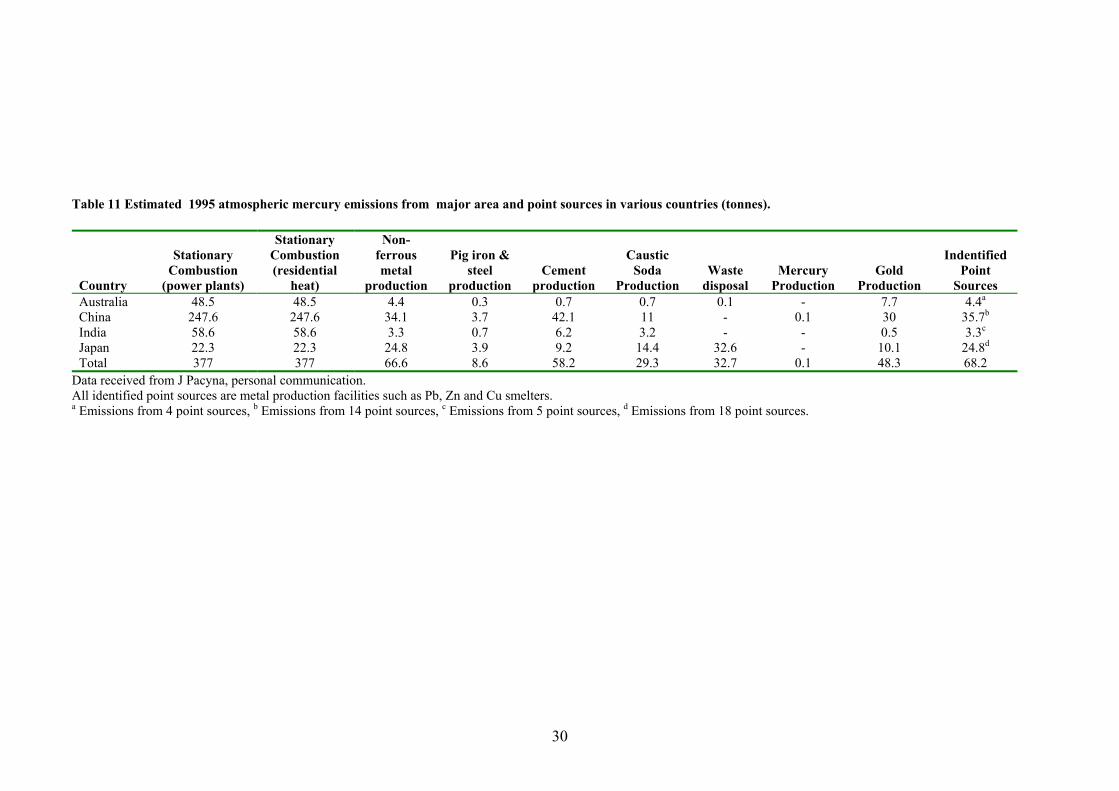
30

Table 11 Estimated 1995 atmospheric mercury emissions from major area and point sources in various countries (tonnes).

Country

Stationary

Combustion (power plants)

Stationary Combustion (residential

heat)

Non-ferrous metal

production

Pig iron &

steel production

Cement production

Caustic

Soda Production

Waste disposal

Mercury Production

Gold Production

Indentified

Point Sources

Australia 48.5 48.5 4.4 0.3 0.7 0.7 0.1 - 7.7 4.4a China 247.6 247.6 34.1 3.7 42.1 11 - 0.1 30 35.7b India 58.6 58.6 3.3 0.7 6.2 3.2 - - 0.5 3.3c Japan 22.3 22.3 24.8 3.9 9.2 14.4 32.6 - 10.1 24.8d Total 377 377 66.6 8.6 58.2 29.3 32.7 0.1 48.3 68.2

Data received from J Pacyna, personal communication. All identified point sources are metal production facilities such as Pb, Zn and Cu smelters. a Emissions from 4 point sources, b Emissions from 14 point sources, c Emissions from 5 point sources, d Emissions from 18 point sources.

31

3.4.2 2001 Australian mercury emission inventory

The Australian continent is rich in natural resources such as bauxite, coal, iron ore, copper, tin,

uranium, nickel, tungsten, mineral sands, lead, zinc, diamonds, natural gas, and petroleum (ABS,

2002b & d). The economy is strongly resource based and commodities such as fossil fuels,

minerals, metals, and agriculture products account for 57 percent of the value of the total export

earnings (ABS, 2002d & e). Anthropogenic Hg emission levels are enhanced in the process of

extraction and treatment of natural resources, such as metal production, as well as by reliance on

fossil fuel combustion for electricity generation. Since fossil fuel combustion accounts for

approximately 90 percent of Australian electricity generation capacity and plays an important role

in servicing the needs of energy intensive commodity production such as aluminium, steel and

iron (ABS, 2002d & e), a large proportion of Australian anthropogenic Hg emissions originate

from these types of activities.

The following Hg emission inventory in Australia is divided into two parts. The first part deals

with point sources (i.e. for a defined industry locations with known latitude and longitude

coordinates for each Hg source), where raw data for Hg emissions has been provided to the

Australian National Pollution Inventory (NPI, 2003a). In the second part, emissions from area

sources (i.e. Hg sources with no specific location), which were calculated as part of the NPI, on

the basis of emission factors (mass Hg per unit product) and statistical data concerning amount

consumed/produced of each product are discussed. Thus, the total Hg emission from Australia

becomes the sum of Hg from these two sources. The total emissions from each source category

are proportioned according to a source profile between the three different Hg species emitted.

Table 12 summarises the estimated Hg emission rates by source type from Australia in

2000/2001.

3.4.2.1 Atmospheric emission from point sources

Identified Australian point sources were estimated to emit about 7.0 tonnes Hgtot/yr (or ~70% of

the estimated total anthropogenic atmospheric emissions in 2000/2001, Table 12, Figure 4). Three

States; Western Australia (WA), Queensland (QLD), and New South Wales (NSW) account for

more than 83 percent of the total Hg emission from point sources to the atmosphere. Point sources

in these States emit, respectively, 2.3 tonnes (33%), 2.0 tonnes (29%) and 1.4 tonnes (21%). The

other 17 percent of the estimated Hg emissions are divided between Victoria (VIC) (6.9 %),

Tasmania (TAS) (4.8 %), South Australia (SA) (3.0 %), Australian Capital Territory (ACT) (1.3

%), and the Northern Territory (NT) (0.5 %) (Figure 4 and Appendix A)(NPI, 2003a).

32

Distribution of Australian anthropogenic Hg emissions geographically and between source

categories are shown in Figures 5 and 6.

Figure 4 Estimated mercury emissions to air (point sources) from States and Territories in Australia 2000/2001 (kg/yr).

Figure 5 Estimated mercury to air (point sources) by source category in Australia, 2001 (kg/yr).

Electricity generation is a significant component of identified point sources of Hg. The NPI (2003a) estimates that 1.9tonnes (~19% of Australian anthropogenic atmospheric emissions) emanates from this industry.

Point source emission of Hg from Australian States and Territories

0.0

500.0

1000.0

1500.0

2000.0

2500.0

WA QLD NSW VIC TAS SA ACT NT

kg Hg(tot)kg Hg0kg Hg(II)kg Hgp

Emission of Hg by point source type

0

500

1000

1500

2000

Elec

trici

tySu

pply

Alu

min

iaPr

oduc

tion

Stee

l and

met

al

Oth

erIn

dust

ry

Was

teD

ispo

sal

Min

ing

Che

mic

alIn

dust

ry

Oil

and

gas

Hg(total) Hg0Hg(II)Hgp

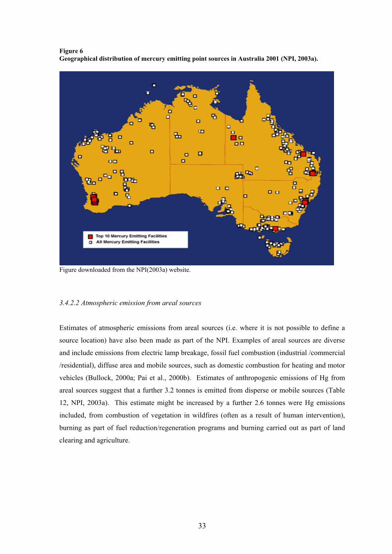
33

Figure 6 Geographical distribution of mercury emitting point sources in Australia 2001 (NPI, 2003a).

Figure downloaded from the NPI(2003a) website.

3.4.2.2 Atmospheric emission from areal sources

Estimates of atmospheric emissions from areal sources (i.e. where it is not possible to define a

source location) have also been made as part of the NPI. Examples of areal sources are diverse

and include emissions from electric lamp breakage, fossil fuel combustion (industrial /commercial

/residential), diffuse area and mobile sources, such as domestic combustion for heating and motor

vehicles (Bullock, 2000a; Pai et al., 2000b). Estimates of anthropogenic emissions of Hg from

areal sources suggest that a further 3.2 tonnes is emitted from disperse or mobile sources (Table

12, NPI, 2003a). This estimate might be increased by a further 2.6 tonnes were Hg emissions

included, from combustion of vegetation in wildfires (often as a result of human intervention),

burning as part of fuel reduction/regeneration programs and burning carried out as part of land

clearing and agriculture.

34

3.4.2.3 Total Australian anthropogenic emission

The total anthropogenic Hg emission from Australia in 2000/2001, including point and area

sources (but excluding burning of vegetation), going to air, land and water was estimated to be

about 10.2 tonnes (Table 12), (NPI, 2003a). Of this 9.9 tonnes is emitted to the atmosphere and

comprises about 0.5 percent of the estimated global anthropogenic atmospheric Hg emissions24.

There is a significant difference apparent between the NPI (2003a) estimate of total annual

Australian anthropogenic atmospheric emissions of 9.9 tonnes for 2000/2001 and the 1995

estimate made by Pacyna and Pacyna (2002) of 110.9 tonnes (Table 11).

Table 12 Distribution of total estimated Australian anthropogenic mercury (kg) for 2001 (NPI 2003a)

Total Air Land Water Identified point sources 6959 6701 54 204 Areal Sources 3210 3210 Total Area and Point Sources 10169 9911 54 204 Burning (including wildfires) 2600 2600 Total all possible sources 12769 12511 54 204

3.4.2.4 Accuracy of emission estimates

A number of scientific studies have attempted to quantify anthropogenic Hg emissions on both

regional (Bullock, 2000a; US EPA, 1997; Pacyna et al., 2001; Pai et al., 2000b; Pilgrim et al.,

2000; Lee et al., 2001) and global scales (Pacyna and Pacyna, 2002; Pirrone et al., 1996, 2001b).

Although there have been an increasing number of Hg emission inventories published, there are

still many uncertainties surrounding estimates of anthropogenic emissions (Bullock, 2000b). As

stated previously, in the latest published study on global emissions, the total atmospheric Hg flux

from Australia in 1995 was estimated to be at least 110.9 tonnes/yr (Table 11) (Pacyna and

Pacyna, 2002). However, according to an earlier study, the emission rate of Hg in Australia was

suggested to be 35 tonnes/yr (based on 1992) (Pirrone et al., 1996), i.e. one third of the later

estimate. Moreover, if the emission of Hg in the Pacyna and Pacyna (2002) study is compared to

the latest NPI (2003a) figures the difference in estimated emission fluxes is even larger (by a

factor of nearly 11).

The large variances in suggested emission fluxes between different studies appear, amongst other

things, to be due to the fact that most of the investigations conducted use emission factors (EF) for

each source category in terms of mass of Hg emitted per unit of fuel consumed or product

produced. These emission factors may be either based on direct measurements of gases

discharged, or on expert judgments, both of which need take into account the Hg content in the

35

raw material, the technology of the industrial process, and the type of abatement technology.

Assuming that suitable representative sample techniques, sampling locations (i.e. allowing typical

sample output in the stack to be determined) and appropriate analytical techniques are applied,

emission factors based on direct measurements are considered to be more accurate than emission

factors derived from expert judgments (Pacyna et al., 2001; Pai et al., 2000b). However, a major

uncertainty associated with direct measured-emission factors can be caused by extrapolation of

measurements conducted at a limited number of facilities with specific production conditions to

generalize across an industry. For instance, for an inventory in the US, an emission factor based

on 10 measurements was used to estimate emissions from 200 different waste incineration plants

that burnt different kind of fuels (Pai et al., 2000b).

Since in many cases, it is impossible to carry out in situ measurements some other sort of

assumption and validation/judgement needs to be made to estimate individual emissions. As

always, assumptions can introduce substantial biases in the estimated Hg emission from a specific

facility or source category, which consequently affects the end result. The US EPA (1997) for

example estimated the Hg emission from fuel oil combustion in the US to be 10 tonnes/yr.

According to Wilhelm (2001) this value was based on an emission factor that overestimates the

Hg concentration in fuel oils by a factor of 3 - 10. Thus, the actual Hg emission is, according to

Wilhelm (2001), probably in the range of 1 - 3 tonnes/yr.

In the study by Pacyna and Pacyna (2002) and Pacyna et al., (2001) a range of emission factors

were used. They concluded that the following accuracy of emission estimates can be assigned to

the different source categories:

• stationary fossil fuel combustion: ± 25 %

• non-ferrous metal production: ± 30 %

• iron and steel production: ± 30 %

• cement production: ± 30 %

• waste disposal: a factor of up to 5

A further source of uncertainty associated with emission inventories, is error by omission, which

occurs due to lack of specific information of particular source categories. For example, in the

inventory of anthropogenic Hg emissions in North America, the category "non-ferrous metal

smelting" for the US, a potential major Hg source, was excluded due to lack of data (Pai et al.,

24 Assuming an average global anthropogenic emission of total mercury of approximately 2 000 tonnes/yr (Bergan et al., 1999; Pacyna and Pacyna, 2002).

36

2000). The US EPA (1997) concluded that if the missing emission sources were added to the

calculations in their study, they could increase the total estimated amount of emitted Hg by as

much as 20 percent.

As previously mentioned there are significant differences between the data collected in the

NPI (2003a) and the estimation by Pacyna and Pacyna (2002) (PP) of anthropogenic atmospheric

Hg emissions from Australia. The most obvious differences lie in estimates of Hg emissions from

combustion of fossil fuels. PP suggest that the total emission of Hg from stationary combustion of

fossil fuels (mostly coal) in Australia is 97 tonnes/yr (1995). An alternative estimate of Hg

emissions from total fuel combustion using data for all Australian fuel sources (ABARE, 2003)

and the emission factors used in the NPI (for differing energy sources, 1999b, 2003b) calculates

that this value should be a maximum of 7.0 tonnes for the year 1995 (Figure 7). By comparison

the calculated emissions using the same data and the PP emission factors for coal gives an

estimate of total Hg emission from all fuel combustion of 111.7 tonne.

Figure 7 Estimates made using NPI (1999b, 2003b) emission factors of Australian anthropogenic atmospheric mercury emissions from fuel and coal combustion compared with emissions which arise from combustion during electricity generation

0

1

2

3

4

5

6

7

8

9

1990 1992 1994 1996 1998 2000 2002 Reporting Year

Mer

cury

Em

issi

on (t

onne

s)

All fuel sources

Electricity generation

All coal and coal products

The difference in the 1995 values can be explained as being simply due to the use of differing

emission factors during calculation. For example, PP used an emission factor of

37

1.0E-03(tonne/ktonne) or 1000ppb for coal (Pacyna and Pacyna, 2002), whereas the NPI(1999b)

uses 4.2E-05 (tonne/ktonne)(42ppb). The use of the latter value can be justified on the basis of

the work of Dale(1999), who found that the trace Hg content of Australian coals was in the range

16-76 ppb, with a mean of 44 ppb. It is also known that the actual level of emissions may be also

be further diminished during the combustion process as 5 - 30 percent of the Hg can be captured

by the fly ash and is consequently not emitted to the atmosphere (Levin (EPRI), 2001). The Hg

concentration in the flue gas may be even further reduced due to the application of various

abatement technologies, although power plants in Australia currently have no such systems

installed. Thus it is possible to calculate that the total Hg emissions from coal combustion for

1995 could have been as low as 3.2 tonnes ( assuming 30% of coal emissions were trapped in the

flyash), but it is inconceivable that it could have been as high as 97 tonnes.

Using the NPI (1999b, 2003b) emission factors, the value calculated for Hg emitted from all fossil

fuel combustion for the 2000/2001 year is 8.4 tonnes (Figure 7). This result compares favorably

with the values calculated in the NPI (2003a) for Hg emissions in that year (Table12), given that

fossil fuel combustion, in various forms, is the major mechanism for anthropogenic Hg release.

Even so there remain apparent discrepancies between the calculations of Hg emissions using

Australian national consumption figures (for example fuel used in electricity generation) and

those generated in the NPI (2003a) which uses the sum of values calculated at the individual plant

(point source) level. For the 2001 reporting year these results were 5.1 tonnes and 1.9 tonnes

respectively. This discrepancy is being investigated as part of the ongoing CCSD project on

emissions.

As further evidence to support the view that the lower NPI calculated emission rate is more

reasonable, a country-by-country comparison, has been conducted. In this comparison the

calculated anthropogenic emission flux of Hg in each country was divided by their respective

population. The Australian per capita emission of Hg is, depending on whether the emission flux

is 110.9 (PP) or 9.9 tonnes/yr (NPI, 2003a), 5.66 or 0.51 g Hgtot/capita/yr, respectively. The latter

value compares favorably to values for other countries which range from 1.46 (Czech Republic)

to 0.10 g Hgtot/capita/yr (Sweden) (Table 13). Thus, the emission rate of 110.9 tonnes/yr as

suggested by PP seems again, based on the results from the per capita emission comparison,

unrealistically high.

38

Table 13 Country-by-country comparison based on anthropogenic atmospheric Hgtot/capita.

Country

Hg (total) (tonnes/yr)

Populationa (million)

g Hgtot/capita

Reference

Czech Republic 15 10.3 1.46 Pacyna et al., 2001 Japan 139.6 127.3 1.09 Pacyna and Pacyna, 2002 Canada 33.2 31.0 1.07 Bullock, 2000a Romania 23 22.4 1.03 Pacyna et al., 2001 Poland 33.6 38.6 0.87 Pacyna et al., 2001 Ukraine 36 49.1 0.73 Pacyna et al., 2001 USA 176 285.9 0.62 Pai et al., 2000b Russia 87.7 144.7 0.61 Pacyna et al., 2001 Australia 9.9 19.6 0.51 NPI 2003a Australiab 110.9 19.6 5.66 Pacyna and Pacyna, 2002 China 616.0 1285 0.48 Pacyna and Pacyna, 2002 Europe 249.7 582.2 0.43 Pacyna and Pacyna, 2002 Germany 31.3 82 0.38 Pacyna et al., 2001 Global averagec 2200 6134 0.36 This study France 17.6 59.5 0.30 Pacyna et al., 2001 UK 127 59.5 0.21 Lee et al., 2001 India 131.1 1025 0.13 Pacyna and Pacyna, 2002 Sweden 0.9 8.8 0.10 Pacyna et al., 2001

a From the State of the World, 2001. http://www.unfpa.org/swp/2001/english/indicators/indicators2.html. b This figure is from the investigation of Pacyna and Pacyna 2002, indicating the unrealistic high emission that is estimated from Australia. c Emission based on Bergan and Rhode, 2001; Pacyna and Pacyna, 2002

The PP study also estimates the combined Hg emissions from non-ferrous metal production (Cu,

Pb, Zn), pig iron/steel production and cement production in Australia (1995) to be approximately

5.4 tonnes/yr (Table 11), which is a factor of about three higher than that estimated by the NPI

(2003a) [1.7 tonnes/yr for (2000/2001)](Table 14). This figure from PP also appears to be in

error, given that the economic mix has not changed substantively in the period. It should however

be noted that the absolute difference in these values is relatively small when compared to the

difference between estimates of Hg emissions from coal combustion.

To further investigate these differences the emission rates of Hg from the three source categories

(non-ferrous metal production (Cu, Pb, Zn), pig iron/steel production and cement production)

were calculated using the EF in the PP study (Pacnya and Pacyna 2002) and statistical production

data from Australia (2001). The calculations are shown in Appendix B. The results show that if

the calculated emissions, (using the PP emission factors), from the three source categories are

compared to the NPI emission data, 11.1 tonnes rather than 2.0 tonnes of Hg is calculated to be

released annually from Australia from these sources. Thus it is apparent that depending on which

emission estimation technique is being used, including the choice of EF and statistical data,

significant discrepancies can occur between calculated emission results.

39

3.4.2.5 Estimation of mercury speciation

As discussed previously the speciation of Hg (i.e. the fraction of Hg0, Hg(II) and Hgp in the total

emission) strongly affects its transportation, atmospheric residence time and deposition pathways

through the atmosphere. In order to investigate the potential environmental effects of Hg, the

dispersion and deposition, and the contribution of elemental Hg to the global atmospheric pool,

the estimated total Hg emission from Australia was divided between the three different species

(Hg0, Hg(II), Hgp). This division is achieved using an estimation of the speciation of the Hg

emitted from various sources and processes. In Table 14, a number of speciation profiles are listed

based on source categories. Thus, depending on the source a speciation profile is assigned and the

distribution between the species can be calculated (Table 15).

Of the approximately 9.9 tonnes of anthropogenic Hg released to the atmosphere annually in

Australia, it is estimated that about 9.9 tonnes is emitted into the atmosphere, it is calculated that

4.75 tonnes (48 %) are in the form of elemental Hg, 1.30 tonnes in the form of divalent Hg

(13 %), and 3.88 tonnes (39 %) is in the form of particulate Hg. The Hg0 is therefore available to

enter the global atmospheric pool each year, this constitutes about 0.5 percent of the increase in

the annual global anthropogenic Hg pool, based on an increasing pool of about 1000 tonnes per

annum (Pacyna and Pacyna, 2002). The remaining emissions of Hg (~5.0 tonnes) are assumed

to be deposited on a local to regional scale. Deposition is discussed in more detail in Section 4.

40

Table 14 Emission speciation (fraction of the total) of mercury from anthropogenic sources Sources Hg0 Hg(II) Hgp Reference

Chemical production: 0.8 0.1 0.1 1 Industrial chemicals (general) Chlor-alkali production: 0.7 0.3 0 1 Industrial chemicals (general) Electric utilities: 0.5 0.3 0.2 1 Electric power generation Iron and steel production: 0.8 0.1 0.1 1 Coke and gas Iron and steel production Iron ore mining and beneficiation Steel foundries Pig & iron 0.8 0.15 0.05 2 Non-ferrous metal smelting: 0.8 0.1 0.1 1 Copper smelting & refining (base metal smelting) Copper smelting & refining (mining, milling and conc.) Non-ferrous smelting and refining (miscellaneous) Lead smelting & refining Zinc smelting & refining Lead and Zinc 0.8 0.15 0.05 2 Cement manufacturing: 0.8 0.1 0.1 1 Cement and concrete industry Cement production 0.8 0.15 0.05 Waste combustion: 0.2 0.6 0.2 1 Commercial incineration Municipal incineration Waste incineration 0.2 0.6 0.2 2 Fossil fuel combustion: 0.5 0.3 0.2 1 Commercial fuel combustion Electric power generation Residential combustion Coal and oil combustion 0.5 0.4 0.1 2 Medical waste incineration: 0.02 0.73 0.25 1 Biomedical waste incineration Non-medical waste incineration: 0.2 0.6 0.2 1 Commercial incineration Municipal incineration Sewage sludge incineration High temperature fabrication: 0.8 0.1 0.1 1 Aluminum oxides (abrasives manufacturing) Ferro-alloys manufacturing Glass manufacturing Non-ferrous smelting and refining misc. Caustic soda 0.7 0.3 0 2 Average of all sources, Europe 1995 0.64 0.285 0.075 2 Average of all sources, Global, 1995 0.53 0.37 0.10 4 Average of all sources, Northern Hemisphere, 2002 0.58 0.33 0.09 3 Ref. 1: Bullock et al., 2000; Ref. 2: Pacyna et al., 2000; Ref. 3:Pacyna and Pacyna, 2002; Ref.4: Travnikov and Ryaboshapko, 2002.

41

Table 15 Estimates of Australian atmospheric mercury emission rates by source 2001 (NPI, 2003a) Identified Point Sources Hg(total) % of Hg0 Hg(II) Hgp

kg/yr total kg/yr kg/yr kg/yr Alumina Production 1789.0 26.7 1431.2 178.9 178.9 Aluminium Smelting 5.3 0.1 4.2 0.5 0.5 Basic Iron and Steel Manufacturing 386.1 5.8 308.8 38.6 38.6 Basic Non-Ferrous Metal Manufacturing n.e.c. 358.4 5.3 286.7 35.8 35.8 Bauxite Mining 9.9 0.1 7.9 1.0 1.0 Black Coal Mining 88.7 1.3 71.0 8.9 8.9 Cement and Lime Manufacturing 290.4 4.3 232.3 29.0 29.0 Chemical Product Manufacturing n.e.c. 125.1 1.9 100.1 12.5 12.5 Clay Brick Manufacturing 17.9 0.3 14.3 1.8 1.8 Copper Ore Mining 7.6 0.1 6.1 0.8 0.8 Copper, Silver, Lead and Zinc Smelting, Refining 966.9 14.4 773.5 96.7 96.7 Dairy Product Manufacturing n.e.c. 66.0 1.0 52.8 6.6 6.6 Electricity Supply 1903.0 28.4 951.5 570.9 380.6 Fertiliser Manufacturing 2.1 0.03 1.7 0.2 0.2 Glass and Glass Product Manufacturing 9.1 0.1 7.3 0.9 0.9 Gold Ore Mining 17.7 0.3 14.2 1.8 1.8 Hospitals (Except Psychiatric Hospitals) 20.5 0.3 16.4 2.0 2.0 Inorganic Industrial Chemical Manufacturing n.e.c. 70.4 1.1 49.3 21.1 0.0 Iron Ore Mining 29.2 0.4 23.3 2.9 2.9 Meat Processing 3.0 0.0 2.4 0.3 0.3 Milk and Cream Processing 2.0 0.0 1.6 0.2 0.2 Mining n.e.c. 15.3 0.2 12.2 1.5 1.5 Oil and Gas Extraction 14.2 0.2 11.3 1.4 1.4 Organic Industrial Chemical Manufacturing n.e.c. 4.3 0.1 3.5 0.4 0.4 Paper Product Manufacturing n.e.c. 2.1 0.0 1.6 0.2 0.2 Paper Stationery Manufacturing 7.0 0.1 5.6 0.7 0.7 Petroleum and Coal Product Manufacturing n.e.c. 3.7 0.1 2.9 0.4 0.4 Petroleum Refining 68.6 1.0 54.9 6.9 6.9 Plaster Product Manufacturing 3.0 0.0 2.4 0.3 0.3 Pulp, Paper and Paperboard Manufacturing 27.4 0.4 21.9 2.7 2.7 Silver-Lead-Zinc Ore Mining 77.7 1.2 62.1 7.8 7.8 Sugar Manufacturing 18.5 0.3 14.8 1.8 1.8 Waste Disposal Services 271.9 4.1 54.4 163.1 54.4 Other sources (n.e.c.) 19.6 0.3 15.7 2.0 2.0 Total (Point source, Air only) 6701 100 4620 1201 881

Anthropogenic Areal Sources Hg(total) % of Hg0 Hg(II) Hgp kg/yr total kg/yr kg/yr kg/yr

Paved/Unpaved roads (particulates) 2800 87.2 0 0 2800 Fuel combustion (sub reporting threshold) 180 5.6 90 54 36 Windblown particulates 140 4.4 0 0 140 Motor Vehicles 66 2.1 33 19.8 13.2 Domestic fuel combustion 7.9 0.2 3.95 2.37 1.58 Other 16.1 0.5 8.05 4.83 3.22 Total of Areal Sources (to Air) 3210 100 135 81 2994 Total Area & Point Sources ( to Air) 9911 4755 1282 3875 The data in column 1 is proportioned between the three different Hg species according to the speciation profile listed in Table 13.

42

4. DEPOSITION OF MERCURY

The most important delivery process of Hg to terrestrial and water compartments is deposition

from air via wet and dry processes (Fitzgerald et al., 1991; Lindquist et al,. 1991; Slemr et al.,

1985). The relative importance of these processes depends on the following factors: (i) the

chemical form of the pollutant (assumed in this study: to be Hg0/Hg(II)/Hgp), (ii) the solubility of

the pollutant in water (iii) the amount of precipitation in the region, and (iv) the characteristics of

the land and surface cover (Seinfeld and Pandis, 1998).

Dry deposition of gaseous species and particles refers to atmospheric removal processes, which

do not include precipitation. The factors that, in general, govern the dry deposition processes are

(i) the physio-chemical properties of the deposited pollutant, (ii) the characteristics of the surface,

and (iii) the level of atmospheric turbulence. The level of atmospheric turbulence effects the rate

at which a pollutant is transported through the atmosphere. This is particularly the case in the air

layer closest to the ground. For gaseous species, properties such as solubility and reactivity affect

their interaction with other species and media in the atmosphere, as well as uptake at the receiving

surface. For particles; shape, size and density affect their transportation via the atmosphere and

whether or not they are adhering to a surface. The shape and cover of the surface itself is also a

factor that affects the process of dry deposition. For instance, a non-reactive surface does not

promote dry deposition since it resists adsorption/absorption of a gaseous species. Furthermore, a

smooth surface may prevent the capturing of particles. However, most natural surfaces, generally,

promote dry deposition (Seinfeld and Pandis, 1998).

Wet deposition of atmospheric contaminants refers to the removal process associated with

precipitation (i.e., when contaminants are incorporated into precipitation elements (clouds, rain

droplets, and aerosols), which subsequently fall to the ground). The wet deposition process is

regarded as highly complex. Due to its complexity, wet deposition is not included in this study.

In Section, 4.1, the theory behind dry deposition will is reviewed, Section 4.2 looks at the

deposition patterns of Hg species, and in Section 4.3, a dispersion and deposition study conducted

over the central, coastal part of NSW is presented.

43

4.1 Dry Deposition

Dry deposition is usually described with a single parameter; the deposition velocity (vd) (ms-1),

which consists of two components; diffusion and gravitational settling. Gaseous species are

assumed to have zero gravitational settling velocity due to their negligible molecular weight,

whereas particles, in general, have both diffusion and gravitational settling components. In the

following paragraphs, two equations which are used in calculating the deposition velocity are

presented; one for gaseous pollutants, and one for particles. References to this section can be

found in Finlayson-Pitts and Pitts (2000), and Seinfeld and Pandis (1998).

In modelling dry deposition using vd, it is assumed that the rate of deposition per unit area; F

(µgm-2s-1) is proportional to the concentration of the deposited species, at a reference height (z)

above the surface:

F = - vd×C(x,y,z) (1)

By using a single parameter (vd) to describe the whole variety of physical and chemical processes,

whereby pollutants may be transported and removed from the atmosphere to a surface, the model

simulations are simplified. Thus, as long as the deposition velocity and the concentration of the

pollutant are known, the deposition flux can be calculated in any geographical location. The

disadvantage with excluding chemical and physical processes that affects the interactions between

atmospheric constituents and media is that it becomes difficult to choose a representative

deposition velocity. Most studies, however, use default values for vd (Table 16).

The process of dry deposition of a pollutant is generally described in three steps: (i) aerodynamic

transport down through the atmosphere to the vicinity of the surface, (ii) crossing of a stagnant

sublayer, called the quasi-laminar sublayer, via either molecular (for gases) or Brownian (for

particles) diffusion, and finally (iii) uptake at the surface. Each of the described steps determines

the value of the deposition velocity.

As the pollutant is transported from the atmosphere to the surface (via step i-iii) it experiences a

number of so-called resistances which affect the magnitude of its deposition rate and hence its

deposition fluxes. Assuming that the deposition flux is independent of height, a resistance, r, can

be defined for each of the above mentioned steps, that is, for each zone that the pollutant has to

cross:

44

r(z2,z1) = C(z2) – C (z1) (2)

F

The deposition velocity for gaseous species is defined as:

vd = 1/r (3)

where r can be broken down into three resistances:

r = ra + rb + rs (4)

1. ra is the aerodynamic resistance determined by the vertical eddy diffusivity, which in turn

depends on the meteorology and the surface roughness. Except in the case of large particles

where gravitational settling must be taken into consideration (see below), ra is independent of

the physical form of the pollutant.

2. rb is the sub-layer resistance (i.e., the resistance to cross the thin layer in the vicinity of the

surface). A variety of mechanisms such as the physical form of the species and the

characteristics of the surface affect the transport across this layer. The resistance ra, together

with rb, are effected by wind speed, vegetation height and atmospheric stability. The sum of

the two resistances tend, in general terms, to decrease with increasing wind speed and

vegetation height. Thus, the resistance is lower (i.e., vd is higher) over forests than over grassy

areas. In daytime, ra is relatively low whereas it is considerably higher and often the

controlling factor for vd during the night, when turbulent mixing is reduced.

3. rs is the surface resistance which is, as for rb, determined by the characteristics of the

receiving surface as well as by the properties of the pollutant. The resistance that is offered by

different surfaces to dry deposition generally depends on the level of moisture and pH of the

surface, and on the solubility and reactivity of the gaseous species.

45

Table 16 Dry deposition velocity of mercury species (cm/s)

Hg0 Hg(II) Hgp Reference 0 0.5 0.025 Petersen et al. 1995a 0.03 (May-Oct) 0.01 (Rest of the year)

0.5 - Ryaboshapko et al. 2000b

0.03d (warm season) 0.01d (Temp. 8-10 0C)

0.3 (Day) 0.15 (Night)

- Bergan et al. 1999c, Bergan and Rohde, 2001d

0.06 2.9 (average, day) 0.3 (night)

0.2 (day) 0.02 (night)

US EPA, 1997e

a No temporal or spatial variability of vd. b Used in a regional Eulerian model (Europe) where dry deposition is only included over land. If the surface air temperature is negative, no dry deposition of Hg0 is assumed. The deposition velocity of Hg(II) is also assumed to be independent of season and surface cover. c A study of the global distribution of Hg0 and Hg(II) using a climatic transport model. Dry deposition is mainly assumed to affect Hg(II). No seasonal variation of vd is included. d This work is revision of the study by Bergan et al. 1999. The same dry deposition rate of Hg(II) is used. Dry deposition of Hg0 is added to the reference case in order to investigate the sensitivity of the model. e A comprehensive assessment concerning Hg where, among other things, dry deposition is modeled using a Lagrangian-type simulation model (RELMAP) (regional basis, dry deposition of Hg0 is excluded) as well as a so-called ISC3 model for predicting deposition 50 km from the emission source (including dry deposition of Hg0).

The deposition velocity of particles is similar to that of gaseous compounds except that particles

are also subjected to a gravitational settling velocity (vs). Thus, by rearranging Equation (3)

(which is described in more detail in Seinfeld and Pandis (1998)), assuming rs = 0 (particles

adhere upon surface contact) the following vd is derived:

vd =(1/(ra + rb + rarbvs)) + vs (5)

Thus, since the deposition velocity is the reciprocal of resistance, each individual resistance term

sets a boundary on the rate of deposition. However, as previously mentioned, many studies use

default values for vd. In Table 16, a number of vd of Hg species are listed.

4.2 Deposition patterns of mercury

Until recently it was assumed that dry deposition of elemental Hg was only a minor portion of the

total amount of Hg deposited. In recent published simulation studies, however, dry deposition of

elemental Hg is often included in the calculations. The reason is that, even if the deposition

velocity of Hg0 is low (Table 16), the significant amount of Hg0 present in the atmosphere may

still have an important effect on the overall deposition flux of Hg to environmental surfaces. For

46

instance, in a comprehensive data simulation study in the US, it was concluded that approximately

25 % of the total deposition of Hg is in the form of dry deposition of Hg0 (Xu et al., 2000a,b)25.

The different Hg species deposition pathways are described in more detail in Sections 2 and 5. In

essence, Hg(II)(g) is removed from the atmosphere in three ways (i) it may condense onto

particulate material, which are either scavenged by atmospheric water droplets or dry deposited to

the surface, (ii) it may, in the presence of precipitation, dissolve in the aqueous phase, and hence

undergo wet deposition, and/or (iii) it may dry deposit. Particulate Hg is, as Hg(II), readily

removed from the atmosphere via both wet and dry deposition. Elemental Hg, on the other hand,

is, due to its low solubility and high vapour pressure, not as efficiently removed from the

atmosphere. Even if elemental Hg is not as efficiently removed as Hg(II) and Hgp, it is, still

removed from the atmosphere, either by, (1) transformation to divalent Hg (subjected to (i)-(iii))

and/or (2) dry deposition, which may be a significant removal pathway for Hg0 from the

atmosphere.

Divalent Hg is the predominant form of Hg deposited to the surface (Lindquist et al., 1991). It had

been assumed that wet deposition was the main removal mechanism of Hg(II) from the

atmosphere. However, more recent studies have shown that dry deposition of Hg(II) may be an

equally important (or more important) removal mechanism, even in areas which have relative

high levels of precipitation (Rea et al., 2000; Vette et al., 2002; Landis et al., 2002a,b). A similar

result was obtained in the study by Xu et al (2000a,b), where dry and wet deposition of Hg(II)

constituted 35 and 30 % of the total simulated deposition of Hg, respectively.

These results indicate that a major part of the total deposited Hg may consist of dry deposited

elemental and divalent Hg.

25 The simulation study by Xu et al. (2000a,b) is based on a comprehensive three-dimensional regional scale Eulerian air quality model that incorporates mercury chemistry, in-cloud transformation processes, and air-surface exchange processes. The bi-directional air-surface exchange was use to model emission of Hg0 and dry deposition of Hg from/to natural surfaces. The simulation include Hg0, Hg(II), and Hgp. A background concentration was assigned to each of the three Hg species.

47

4.3 Model simulation

4.3.1 The model

TAPM (The Air Pollution Model) (developed by CSIRO Atmospheric Research, Australia) is a

three-dimensional regional scale Eulerian air quality model, connected to databases for

meteorology, terrain and vegetation. Its dispersion module (which is used in this study) includes

not only an Eulerian grid module, but also an optional Lagrangian particle module for predicting

concentrations of various species near the source (the combination of the two modules are used in

this simulation). Emission data is added either as point or area sources. Information about

TAPM's general theoretical consideration, reference studies and technical descriptions can be

found in Hurley (2002a, b) and Hurley et al., 2002.

Since TAPM is primarily developed to investigate the air quality of an airshed in relation to SOx,

NOx and photochemical smog (including chemical transformations and deposition mechanisms

related to these pollutants), Hg is modeled as an inert pollutant (so-called tracer) where chemical

transformation processes, as well as, deposition processes are omitted. Thus, none of the chemical

reactions/interactions described in Section 2 are included in the model.

Even though deposition of Hg is not included in TAPM, dry deposition fluxes are calculated by

post-processing hourly-simulated grid concentration outputs from TAPM according to

Equation (6). Thus, an hourly dry deposition flux is derived from each grid cell using a default

value for the deposition velocity, as described in section 4.1.

F = - vd×C(x,y,10 m) (6)

The deposition velocity for Hg(II)/Hgp is set to be 0.5 cm/s during the day and zero cm/s during

the night. Corresponding values for Hg0 are 0.03 and zero cm/s, respectively.

4.3.2 Simulation procedure

4.3.2.1 Simulation domain and period

The simulation was conducted to model the period of 1st to the 31st of January 2001. The

simulation domain covered a portion of the central, coastal part of NSW, as shown in Figure 8.

There are two meteorological grid domains; the outer has 25×25 grids in the horizontal plane,

48

with grid size of 30 × 30 km, while the inner grid domain has the same number of grids but a grid

size of 10 × 10 km.

In order to obtain a finer resolution with regard to concentration simulations, an outer and an

inner pollution grid domain is used with 97×97 grids in the horizontal plane, with grid size 7.5 ×

7.5 km and 2.5 × 2.5 km, respectively.

The vertically resolution consists of 25 non-uniform layers, with the finest resolution near the

surface (located 10 m above the ground). The top of the modeling domain is 8 km.

Depending on the stack height of the source, emissions of Hg enter somewhere between the first

and the seventh model layer

Figure 8 Geographical distribution of point sources included in TAPM simulation

Number of grid cells The frame of the figure represents the outer grid domain.

2 4 6 8 10 12 14 16 18 20 22 24

2

4

6

8

10

12

14

16

18

20

22

24

Mount Piper PS

Maldon CW

BHP Steel PKW

Orica Chlorine P SYDNEY

Vales Point PSEraring PS Pasminco

Comsteel

Lidell PSBayswater PS

49

4.3.2.2 Meteorological conditions

Meteorological data used in the simulation is from 2001. January is a summer month in Australia

with high average temperatures. Inclusion of rain is an optional parameter in TAPM, but since

wet deposition is excluded from the simulation, so is rain. The prevailing wind direction during

the simulation period was east/northeast.

4.3.2.3 Mercury emission data

For simplicity a facility emission cutoff of 20 kg/yr was used which ensured that more than 90 %

(1282 kg/yr) of the total anthropogenic point emissions in NSW (NPI, 2003a) were embraced by

the simulation. These emissions were divided between elemental and divalent/particulate Hg

according to the source profiles, previously described in Section 3.4.2.3. The emission rate of Hg

is assumed to be constant over every hour of the year. In order to simulate the concentrations and

deposition fluxes of the different Hg species, a specific "tracer" is assigned to each of the two

groups (Hg0 and Hg(II)/Hgp) . Each tracer can then be analysed.

Emissions from natural sources and area sources are not included in the simulations.

The sources of Hg emissions simulated include: combustion of coal (5 power plants), basic iron

and steel manufacturing (2 sources), cement manufacturing (1 source), Cu/Ag/Pb/Zn smelter (1

source), and chemical production (1 source) (Figure 8, Appendix C).

4.3.2.4 Initial and boundary conditions

Background tracer (Hg) concentrations, as well as, boundary conditions (i.e., the amount of Hg

imported from the global Hg pool to the model domain) are set to be zero. Thus, the ambient Hg

concentration and deposition flux derived from the study originates only from the 10 facilities

investigated.

4.3.2.5 Deposition

Wet deposition is not included in the model simulation whereas dry deposition is calculated by

post-processing hourly simulated grid concentrations of Hg, according to Equation (1). By using

default values for the deposition velocity, an hourly deposition flux is calculated for respective

grid cell and Hg species in the entire domain. Based on the result, an average hourly deposition

50

flux for each grid cell is calculated. These average hourly deposition fluxes are then integrated

over year 2001.

The choice of deposition velocity for each Hg species is based on the information shown in Table

15. Since divalent and particulate Hg are, due to practical considerations, combined in one

category, the chosen velocity represents a weighted average of Hg(II) and Hgp rates. The

deposition velocity of divalent/particulate Hg is assumed to be 0.5 cm/s during day time (12

hours) while at night, due to reduced turbulent mixing (high ra, Section 4.1), it reduces to zero.

Similarly, the deposition velocity of elemental Hg during the day and night is assumed to be 0.03

and zero cm/s, respectively.

4.3.3 Simulation results

4.3.3.1 The simulation

Three simulations are presented in the current report. The first simulation (Run 10), which

includes all ten Hg emitting facilities (Figure 8), was performed to investigate the ambient ground

Hg concentrations (the first vertical layer in the model; 10 m) (4.3.3.2), as well as the deposition

flux of respective Hg species (4.3.3.3, Table 17) in the entire domain. In addition, a number of

mass balances are calculated to determine the average amount of Hg, as well as the percent of

total Hg that would be deposited at different distances around each facility (and in some case

facilities) (each distance is represented by a square box where the source/sources is/are

approximately in the center of the box).

In the Run 10 model simulation, the real stack height of 5 of the sources is unknown

(Appendix C). In order to investigate possible deposition fluxes of Hg at (i) different stack

heights, and at (ii) different distances around respective source (as in Run 10), two additional

simulations (Runs 20 and 30) were conducted (for the 5 sources). When calculating area average

deposition fluxes around some of the facilities in Run 10, some of the grid cells surrounding the

facilities were, at certain distances, overlapping. In order to separate the different facilities and Hg

species, different tracers were assigned to each source as well as to each Hg species.

4.3.3.2 Ambient Hg concentrations

Table 17 shows a percentile analysis of the simulated Hg concentration results from the grid cells

over the entire domain. Based on the result, it is clear that the contribution of Hg from the 10

facilities included in the simulation is relatively small compared to (i) the assumed background

concentration of elemental Hg in Australia of 1.3-1.4 ng/m3 (Bergan and Rodhe, 2001), and (ii)

51

the measured average total Hg concentration in Northwest Europe and in the Mediterranean

region of 1.6-2.4 ng/m3 (Wängberg et al., 2001).

In order to evaluate the contribution of particulate and divalent Hg from the 10 sources included

in the TAPM simulation, a number of published investigations are presented. In a study conducted

by US EPA (1997), the simulated total concentration of divalent and particulate Hg (over the

lower 48 States) at the 10th, 50th and 90th percentile level was 1.0, 5.6, and 23 pg/m3,

respectively26. Moreover, measurements conducted in Tennessee (US) show that divalent Hg

concentrations vary between 50-200 pg/m3 depending on the distance to the emitting sources

(Linberg and Stratton, 1998). In Europe, measured concentrations of particulate Hg ranges

between 10 (Sweden) and 50 (Germany) pg/m3 (Wängberg et al., 2001). Thus, the simulated

concentrations in this study seem to be in general agreement with the published data.

In Table 17, the minimum concentration level of Hg is zero. A zero level of Hg occurs mostly

over the ocean, both in the inner and outer domain, reflecting the dispersion of Hg with the

prevailing winds (the dispersion is represented in Figure 9 and 10).

Table 17 Percentile Analysis of simulated ambient mercury concentrations

Grid domain

Species

Min pg/m3

10th pg/m3

50th pg/m3

90th pg/m3

Max ng/m3

Inner Hg0 0 7 15 44 2.5 Hg(II)/Hgp 0 2 6 15 0.6 Hgtot 0 9 21 59 3.1 Outer Hg0 0 0 2 14 0.9 Hg(II)/Hgp 0 0 1 5 0.2 Hgtot 0 0 3 19 1.1

The maximum simulated ground level ambient Hg concentration (3.1 ng/m3) is (even if the

background concentration of Hg0 is added), well below (i) the US EPA determined reference

concentration of Hg vapor of 0.3 µg/m3 for the general population (US EPA, 1997), (ii) the limit

value for exposure in Europe of 0.05µg/m3 (Pirrone et al., 2001a)27, and (iii) the proposed air

quality objectives set in Victoria, Australia, of 1.8 µg/m3, for inorganic Hg (VIC EPA, 2002).

26 This study (US EPA (1997)) is, among other things, based on a Lagrangian-type simulation model (RELMAP) as well as a so-called ISC3 model for predicting Hg deposition 50 km from the emission source (including deposition of Hg0). RELMAP is used to investigate the emission, transport and fate of airborne Hg (Hg0, Hg(II), Hgp) over continental US. It incorporates some of the chemistry known to affects the Hg speciation, as well as wet and dry deposition (dry deposition of Hg0 is excluded from the simulation) mechanisms. The background concentration of Hg0 is included in the simulation. 27 According to WHO (2003), a guideline for inhalation of inorganic Hg vapor is established, as an annual average value, in Europe of 1 µg/m3. Thus, it is somewhat higher compared to the limit value reported by (Pirrone et al., 2001a).

52

4.3.3.3 Dry deposition of mercury

Table 18 shows a percentile analysis of simulated dry deposition rates from the grid cells over the

area of study. The simulated total average deposition flux in the inner domain varies between 0.2

and 1.4 µg/m2/yr (at the 10th and 90th percentile level, respectively). In occasional cases, close to

emitting sources (1-2 grid cells away from the source), the deposition flux of Hgtot may reach

levels of 50-60 µg/m2/yr. Corresponding values for the outer domain are smaller as the domain

includes relatively large areas that are unaffected by emitting Hg sources. Similarly, the average

deposition rate for the inner and outer domain is 0.8 and 0.2 µg/m2/yr, i.e. a difference of a factor

of 4.

In order to verify the obtained deposition rates of Hg species in this study, a comparison is made

with simulated dry deposition rates in an earlier US EPA (1997) study. The US study shows that

the simulated total dry deposition flux (excluding elemental Hg) for the lower 48 States in the

USA is, for the 10th, 50th, 90th percentile levels,: minimum 0.05, 0.18, 0.89 and maximum, 5.6 and

62.6 µg/m2/yr, respectively. Thus, the deposition fluxes of Hg in the US study are, compared to

the results in this study, significant higher. One obvious reason for the discrepancy in the

deposition rates of Hg species, is that the lower 48 States of the USA cover approximately the

same land area as Australia, but emit roughly 20 times as much Hg as Australia. A further reason

for the differences in simulated deposition rates may be that the US study used significantly

higher deposition velocities for the Hg species investigated than those used this study (Table 16).

Table 18 Percentile analysis of simulated dry deposition fluxes of mercury species

Grid domain

Species

Min µg/m2/yr

10th µg/m2/yr

50th µg/m2/yr

90th µg/m2/yr

Max µg/m2/yr

Inner Hg0 0.00025 0.033 0.070 0.210 11.6 Hg(II)/Hgp 0.0007 0.155 0.454 1.152 48.4 Hgtot 0.001 0.20 0.55 1.4 60 Outer Hg0 0 0 0.06 0.43 28.7 Hg(II)/Hgp 0 0 0.07 0.41 18.6 Hgtot 0 0 0.14 0.85 48

The outer grid domain includes parts of the ocean, which due to the prevailing wind direction does not experience any dry deposition.

Of the total anthropogenic Hg mass predicted to be deposited to the surface in the model domain,

85 % is estimated to come from divalent/particulate Hg emissions and 15 % from elemental Hg.

In the study by Xu et al (2000a,b), it is estimated that 57 % of the total amount of Hg that is dry

deposited in the model domain came from Hg(II), 6 % from Hgp, and 37 % from Hg0. Thus, the

contribution of Hg0 calculated as a percentage of the total deposition is, compared to this study,

53

somewhat higher. This may be explained by the fact that the Xu et al (2000a,b) simulation

includes the background concentration of Hg0.

If the average simulated deposition rate in the outer domain of 0.2 µg/m2/yr is integrated over the

area of study, approximately 105 kg (~ 8 % of the total emissions from the facilities investigated)

of Hg are deposited annually within the entire domain. The rest of the Hg is transported outside of

the domain and deposited elsewhere.

Since the simulated tracer (Hg) is dispersed with the prevailing winds, which, during this

simulation comes from east/northeast, the major part of the deposition fluxes of Hg can be found

over the mainland, as is shown in Figures 9 and 10. Moreover, it is clear from the contour plots

that the deposition fluxes of Hg are significant higher adjacent to the emitting source, than they

are at a greater distance from the source. This deposition trend is also illustrated in Figure 11,

where the deposition fluxes of Hg are concentrated around specific point sources. Thus, from the

information provided in Figure 11, it is obvious that the area around Comsteel, Pasminco CCS,

Vales Point PS and Eraring PS, would experience the greatest amount of deposited Hg in the

domain. The second and third areas that receive relatively large simulated masses of deposited Hg

are the Orica Chlorine plant and BHP Steel PKW.

In order to investigate (i) the aggregated average amount of Hg, and (ii) the percent of total

emitted Hg that is deposited at different distances around each facility, a number of deposition

calculations are presented. These calculations are based on simulated hourly grid deposition

fluxes of Hg around each facility, as well as on the emission rates of Hg from respective facility.

The result is presented in Tables 19-24 and Appendix D.

It is well-known that the differences in simulated air concentrations and deposition fluxes across a

model domain are mainly dependent on factors such as stack height (real height), the exit velocity

(momentum) of the plume from the stack, and the emission rate of Hg28. Thus, these

factors determine the height to which the plume rises from the stack top (the so-called effective

stack height), and consequently the distance the pollutant is carried before deposition (Cartwright,

1993)29. For example, power plants, which have relatively tall stacks, high exit velocities and

28 Additional factors that determine the effective stack height is wind speed, diameter of the stack, gas exit temperature, ambient temperature, and the atmospheric stability condition. (Cartwright, 1993) 29 The speciation of Hg species is, as previously described, crucial for the deposition patterns of Hg. Thus, atmospheric transformation/interaction processes, which determine the speciation of Hg, are important to include in models aiming at simulating Hg transportation and deposition. In this study, however, none of these processes/interactions are included. Thus, the "only" parameters effecting the dispersion and deposition of Hg, in this study, are the physical characteristics of the emission source and the atmospheric conditions.

54

emission rates, disperse the emitted pollutant further away from the emission point than sources

with the opposite conditions (as will be seen in the following paragraphs). In the model simulation

the actual stack height of five of the ten sources was unknown (Appendix C). In order to

investigate possible deposition fluxes at different stack heights and distances around each facility,

two additional simulations were conducted (Runs 20 and 30). The result of the simulations and

calculations are presented in Tables 19-24 and in Appendix D.

Figure 9 Contour plot of simulates of dry deposition of divalent/particulate mercury (unit: µg/h)

2 4 6 8 10 12 14 16 18 20 22 24

2

4

6

8

10

12

14

16

18

20

22

24

Mount Piper PS

Maldon CW

BHP Steel PKW

Orica Chlorine P SYDNEY

Vales Point PSEraring PS Pasminco

Comsteel

Lidell PSBayswater PS

Number of grid cells

In Tables 19 and 21-22, the area average deposition flux of Hg (12.5×12.5 km) ranges between

0.6-12.4 µg/m2/yr. The highest area (12.5×12.5 km) deposition flux of Hg are to be found around

Comsteel (12.4 µg/m2/yr), Pasminco CCS (12 µg/m2/yr), and the Orica Chlorine plant (8.8

µg/m2/yr). If these area deposition fluxes are calculated as a percentage of the total Hg emission

from respective facility, each Hg deposition flux represents 0.7, 1.7 and 1.1 % of the total Hg

emitted, respectively. However, the stack height of each of these facilities needs to be increased

55

by a factor of 5 (Table 21-22), to decrease the previously calculated fluxes by a factor of

approximately 2.

Figure 10 Contour plot of simulates of dry deposition of elemental Hg (unit: µg/h)

2 4 6 8 10 12 14 16 18 20 22 24

2

4

6

8

10

12

14

16

18

20

22

24

Mount Piper PS

Maldon CW

BHP Steel PKW

Orica Chlorine P SYDNEY

Vales Point PSEraring PS Pasminco

Comsteel

Lidell PSBayswater PS

Number of grid cells

The only source that does not experience a reduction in deposition fluxes of Hg as the height of

the stack is increased, is the Maldon cement works. The reason for this is unclear. One reason

may be that the facility is located in the inland and that it is subject to other atmospheric

conditions than those sources located closer to the coastline.

The highest emission rate of Hg in the model simulation comes from Bayswater power station,

which emits 301 kg/yr. Since Lidell power station (46 kg/yr) is located close to Bayswater power

station, the two sources are included, together, in the area-deposition calculations. The average

deposition flux of Hg in each of the three areas (12.5×12.5 km, 37.5 ×37.5 km and 52.5× 52.5

km), is 1.7, 2.0 and 0.8 µg/m2/yr, respectively (which constitute 0.1, 0.4 and 0.7 % of the total Hg

56

emitted). Thus, as the simulation shows, a significant amount of the emitted Hg is transported

away from their source with the prevailing winds.

Figure 11 The magnitude of dry deposition fluxes from TAPM simulation (unit: µg/h) The height of the plot is proportionally to the deposition flux of divalent/particulate Hg. The western corner in Figure 11 corresponds (since the Figure is tilted) to the northwest corner in Figures 8,9 and 10. The first, second, third and fourth highest deposition flux of Hg corresponds to source/sources (i) Comsteel, Pasminco CCS, Vales Point PS, Eraring PS, (ii) Orica Chlorine plant, (iii) BHP Steel PKW, and (iv) Lidell PS and Bayswater PS, respectively.

As the calculations presented in Tables 19-24 show, the area average deposition flux of Hg,

expressed as a percentage of the total Hg emitted, was in general, relatively small. This suggests

that a significant part of the Hg emitted from the facilities investigated would be transported away

from the domain.

57

Table 19 Area Average Mercury Deposition Rates for each Facility/Facilities

Run 10 Area Average Values of Dry Deposition

Emission Speciation of emission 12.5*12.5

km 37.5*37.5

km 52.5*52.5

km

Facility Name No. Stack height Hg(tot) Hg0 Hg(II)/Hgp Total Hg0 Hg(II)/Hgp Total Hg0 Hg(II)/Hgp Total Hg0 Hg(II)/Hgp

m kg/yr kg/yr kg/yr ugm-2yr-1 ugm-2yr-1 ugm-2yr-1 ugm-2yr-1 ugm-2yr-1 ugm-2yr-1 ugm-2yr-1 ugm-2yr-1 ugm-2yr-1 Mount Piper PS 2 250 45 22.5 22.5 0.6 0.06 0.5 1.0 0.1 0.9 0.5 0.1 0.4 Liddell PS 3 168 46 23 23 Bayswater PS 4 250} 301 150 150 1.7a 0.10 1.6 2.0 0.20 1.8 0.8 0.1 0.7 Comsteel 5 10 282 226 56 12.4 2.4 10.0 Pasminco CCS 6 74 110 88 22 7.8 1.5 6.3 3.3 0.6 2.7 Vales Point PS 7 178 86 43 43 2.1 0.30 1.8 Eraring PS 8 200 164 82 82 3.0 0.50 2.5 Maldon CW 9 10 23 18.4 4.6 2.0 0.3 1.7 2.8 0.4 2.4 N/A N/A N/A BHP Steel PKW 10 10 102 82 20 N/A N/A N/A 3.6 0.6 3.0 N/A N/A N/A Orica Chlorine P 11 10 124 87 37 5.2 1.0 4.2 4.2 0.5 3.7 1.7 0.2 1.5

a Source 3 & 4 is included in each area The deposition rate is simulated in TAPM during January 2001. The deposition flux is then scaled up to cover the whole year In the area 12.5*12.5 km, source 5,6,7 and 8 is located close to each other and some of the grid cells are therefore overlapping when the deposition is calculated. The same occurs for source 9 & 10 in area 37.5*37.5 km. More accurate data concerning these sources can be found in Run 20 and 30. Table 20 Percent of Total Mercury Dry Deposited around each Facility/Facilities

Run 10 Percent of Total Mercury Emissions Dry Deposited Within Each Area

Emission Speciation of emission 12.5*12.5

km 37.5*37.5

km 52.5*52.5

km

Facility Name No. Stack height Hg(tot) Hg0 Hg(II)/Hgp Total Hg0 Hg(II)/Hgp Total Hg0 Hg(II)/Hgp Total Hg0 Hg(II)/Hgp

m kg/yr kg/yr kg/yr % % % % % % % % % Mount Piper PS 2 250 45 22.5 22.5 0.2 0.02 0.2 1.6 0.2 1.4 3.1 0.4 2.7 Liddell PS 3 168 46 23 23 Bayswater PS 4 250} 301 150 150 0.1a 0.01 0.1 0.4 0.05 0.4 0.7 0.1 0.6 Comsteel 5 10 282 226 56 0.7 0.1 0.6 Pasminco CCS 6 74 110 88 22 1.1 0.2 0.9 1.4 0.3 1.1 Vales Point PS 7 178 86 43 43 0.4 0.06 0.3 Eraring PS 8 200 164 82 82 0.3 0.05 0.2 Maldon CW 9 10 23 18.4 4.6 1.4 0.2 1.2 9.4 1.5 7.9 N/A N/A N/A BHP Steel PKW 10 10 102 82 20 N/A N/A N/A 2.7 0.5 2.2 N/A N/A N/A Orica Chlorine P 11 10 124 87 37 0.7 0.1 0.5 2.6 0.3 2.2 3.9 0.5 3.4

a Source 3 & 4 is included in each area

Sources 5,6,7, and 8 are included in this area

Sources 5,6,7, and 8 are included in this area

58

Table 21 Area Average Mercury Deposition Rates for each Facility

Run 20 Area Average Values of Dry Deposition Emission Speciation of emission 12.5*12.5 km 37.5*37.5 km 52.5*52.5 km

Facility Name No. Stack height Hg(tot) Hg0 Hg(II)/Hgp Total Hg0 Hg(II)/Hgp Total Hg0 Hg(II)/Hgp Total Hg0 Hg(II)/Hgp

m kg/yr kg/yr kg/yr ugm-2yr-

1 ugm-2yr-1 ugm-2yr-1 ugm-2yr-

1 ugm-2yr-1 ugm-2yr-1 ugm-2yr-

1 ugm-2yr-1 ugm-2yr-1

Comsteel 5 10 282 226 56 11.8 2.3 9.5 3.4 0.60 2.8 3.0 0.60 2.4 Pasminco CCS 6 10 110 88 22 12.0 2.3 9.7 1.4 0.20 1.2 1.4 0.2 1.2

Maldon CW 9 10 23 18.4 4.6 1.3 0.2 1.1 0.8 0.1 0.7 0.6 0.1 0.5 BHP Steel PKW 10 10 102 82 20 2.3 0.8 1.5 1.6 0.3 1.3 1.8 0.3 1.5 Orica Chlorine P 11 10 124 87 37 8.8 1.1 7.7 2.1 0.3 1.8 1.5 0.2 1.3 The deposition rate is simulated in TAPM during January 2001. The deposition flux is then scaled up to cover the whole year. Table 22 Area Average Mercury Deposition Rates for each Facility

Run 30 Area Average Values of Dry Deposition Emission Speciation of emission 12.5*12.5 km 37.5*37.5 km 52.5*52.5 km

Facility Name No. Stack height Hg(tot) Hg0 Hg(II)/Hgp Total Hg0 Hg(II)/Hgp Total Hg0 Hg(II)/Hgp Total Hg0 Hg(II)/Hgp

m kg/yr kg/yr kg/yr ugm-2yr-

1 ugm-2yr-1 ugm-2yr-1 ugm-2yr-

1 ugm-2yr-1 ugm-2yr-1 ugm-2yr-

1 ugm-2yr-1 ugm-2yr-1

Comsteel 5 50 282 226 56 6.2 1.2 5.0 2.1 0.40 1.7 2.1 0.40 1.7 Pasminco CCS 6 74 110 88 22 2.4 0.5 1.9 0.7 0.10 0.6 1.0 0.1 0.9 Maldon CW 9 50 23 18.4 4.6 1.0 0.2 0.8 0.7 0.1 0.6 0.6 0.1 0.5 BHP Steel PKW 10 50 102 82 20 0.9 0.3 0.6 1.1 0.2 0.9 1.4 0.2 1.2 Orica Chlorine P 11 50 124 87 37 4.2 0.5 3.7 1.4 0.2 1.2 1.0 0.1 0.9 The deposition rate is simulated in TAPM during January 2001. The deposition flux is then scaled up to cover the whole year.

59

Table 23 Percent of Total Mercury Dry Deposited around each Facility

Run 20 Percent of Total Mercury Emissions Dry Deposited Within Each Area Emission Speciation of emission 12.5*12.5 km 37.5*37.5 km 52.5*52.5 km

Facility Name No. Stack height Hg(tot) Hg0 Hg(II)/Hgp Total Hg0 Hg(II)/Hgp Total Hg0 Hg(II)/Hgp Total Hg0 Hg(II)/Hgp

m kg/yr kg/yr kg/yr % % % % % % % % %

Comsteel 5 10 282 226 56 0.6 0.1 0.5 1.7 0.30 1.4 3.0 0.60 2.4 Pasminco CCS 6 10 110 88 22 1.7 0.3 1.4 1.8 0.30 1.5 3.7 0.6 3.1 Maldon CW 9 10 23 18.4 4.6 1.0 0.2 0.8 5.3 0.8 4.5 7.6 1.2 6.4 BHP Steel PKW 10 10 102 82 20 0.3 0.1 0.2 2.2 0.4 1.8 4.7 0.8 3.9 Orica Chlorine P 11 10 124 87 37 1.1 0.1 1.0 2.3 0.3 2.0 3.3 0.4 2.9 The deposition rate is simulated in TAPM during January 2001. The deposition flux is then scaled up to cover the whole year.

Table 24 Percent of Total Mercury Dry Deposited around each Facility

Run 30 Percent of Total Mercury Emissions Dry Deposited Within Each Area Emission Speciation of emission 12.5*12.5 km 37.5*37.5 km 52.5*52.5 km

Facility Name No. Stack height Hg(tot) Hg0 Hg(II)/Hgp Total Hg0 Hg(II)/Hgp Total Hg0 Hg(II)/Hgp Total Hg0 Hg(II)/Hgp

m kg/yr kg/yr kg/yr % % % % % % % % %

Comsteel 5 50 282 226 56 0.4 0.1 0.3 1.1 0.20 0.9 2.1 0.40 1.7 Pasminco CCS 6 74 110 88 22 0.4 0.1 0.3 1.0 0.20 0.8 2.5 0.3 2.2 Maldon CW 9 50 23 18.4 4.6 0.6 0.1 0.5 4.4 0.7 3.7 6.6 1.0 5.6 BHP Steel PKW 10 50 102 82 20 0.2 0.1 0.1 1.4 0.2 1.2 3.7 0.5 3.2 Orica Chlorine P 11 50 124 87 37 0.6 0.1 0.5 1.5 0.2 1.3 2.2 0.3 1.9 The deposition rate is simulated in TAPM during January 2001. The deposition flux is then scaled up to cover the whole year.

60

5. The Chemistry of Atmospheric Mercury

A knowledge of Hg reactions in the atmosphere is critical for modelling its transportation,

transformation, and concentrations throughout the atmosphere as well as for estimating its

deposition fluxes to environmental surfaces. The following section describes some of the

chemical reactions, which take place in the atmosphere along with kinetic data for Hg. In

addition, the residence time (τ) and/or half-life (t1/2) of Hg, which are convenient measures of the

reaction rate, were calculated and are presented for most of the reactions. In the most general

terms, the chemistry of atmospheric Hg involves aqueous phase (e.g., a raindrop or a fog droplet)

and gaseous phase reactions, transitions of elemental Hg (Hg0) and divalent Hg (Hg(II)) species

between the aqueous and gaseous phase, the solid and aqueous phase and also between the solid

and gaseous phase. These reactions and interactions between different atmospheric reactants and

media determine the speciation of Hg, its removal by processes such as wet and dry deposition, as

well as its atmospheric residence time (Schroeder and Munthe, 1998).

Section 5.1 deals with individual chemical reactions in the aqueous phase. In this phase, for Hg,

two simultaneous reactions occur; oxidation of elemental Hg and reduction of divalent Hg. In

addition, different Hg species and other atmospheric reactants partition themselves between the

air and water phases under equilibrium conditions (Figure 12).

Figure 12 Atmospheric mercury chemistry

X - oxidants, Y - reducing agents. Some of the divalent Hg in the water droplet is also adsorbed onto particles.

Hg(II)(g) Hg(II)(aq) Hg0(aq) Hg0

(g)

X(g)

X(aq)

Y(g)

Y(aq)

Wet Deposition

Atmosphere

Environmental surfaces

H2O

Hg0(g) Hg0

(ads)

Hg(II)(ads) Dry Deposition

Dry

/wet

dep

ositi

on

Dry

/wet

dep

ositi

on

Dry/wet deposition

Hg(II)(s)

61

The driving force and the direction of the Hg flux across the interface, which determine the Hg

concentration in the water phase, are partly governed by the redox reactions taking place in the

aqueous and gaseous phase and partly by the Henry's law constant (Pleijel and Munthe, 1995a,b;

Schroeder et al., 1991). For instance, when divalent Hg (Hg(II)(aq)) is reduced to elemental Hg

(Hg0(aq)) it will, due to its lower solubility, partition back into the gas phase. Thus, the Hg

concentration decrease in the water droplet is less and is hence subjected to wet deposition, and

vice versa. This is illustrated in Figure 12.

As shown in Figure 12, reducing agent (Y), oxidant (X) and elemental Hg are divided across the

air/water surface (in equilibrium). Unlike these three groups of reactants, divalent Hg, due to its

low volatility and high solubility, does not generally partition back into the atmosphere

(Hedgecock and Pirrone, 2001).. Thus, Hg(II)(aq) has to be reduced to Hg0(aq)

in order to reach the

atmosphere. In the water droplet, which is sometimes referred to as a chemical reactor (Lin and

Pehkonen, 1998b), reactions between Hg0/Hg(II) and X/Y occurs as well as reactions between X

and Y (and between different reaction products). Depending on the concentration of individual

chemical species, the pH, the liquid water content in the atmosphere, and other meteorological

factors (e.g. temperature and barometric pressure) different reactions temporarily dominate over

others (Lin and Pehkonen, 1997; Seigneur et al., 1994). Thus, the outcome of the reactions is

determined by the prevailing conditions in the water droplet and in the atmosphere. The aqueous

oxidants are (i) ozone, (ii) hydroxyl radical and (iii) chlorine, and the reducing agents are: (iv)

sulfite complexes, (v) hydroperoxide radicals, and (vi) photoreduction of divalent Hg complexes.

Section 5.2 discusses the oxidation of elemental Hg to divalent Hg in the gas phase (right-hand

side of the figure). The following atmospheric oxidants are present - (i) ozone, (ii) hydroxyl

radical, (iii) nitrate radical, and (iv) hydrogen peroxide30. The products of these reactions

(Hg(II)(g)) are removed from the atmosphere in three ways31: (i) they may condense onto

particulate materials, which are either scavenged by atmospheric water droplets or dry deposited

to marine or terrestrial surfaces, (ii) it may, in the presence of precipitation, dissolve into the

aqueous phase (as described above) and/or (iii) it may dry deposit to the earth surface. Thus,

elemental Hg is removed from the atmosphere by transforming to divalent Hg, either by

partitioning into the aqueous phase where it interacts with different constituents (see aqueous

phase reactions), or by being oxidised in the gaseous phase as described in this paragraph.

Furthermore, it may be directly adsorbed onto particles which are either wet or dry deposited, or

30 In addition, reactions with DMM are also summarised in section 5.2.5. 31 Hg(II)(g) enters also the atmosphere from different emitting sources and are consequently subjected to the same removal processes.

62

Hg0(g) is simply dry deposited (at a very low rate) to the ground (left-hand side of Figure 12) (EC,

2001; Porcella et al., 1996; Seigneur et al., 1994, 1998; Schroeder and Munthe, 1998).

The atmospheric chemistry of Hg is diverse and complex, and the review that follows will

therefore necessarily be simplified. Furthermore, it should be mentioned that the scientific

experiments presented are subject to a degree of uncertainty particularly when it comes to the

derivation of kinetic data in association with gaseous oxidation reactions (some of the Hg0 is lost

during the experiments at the walls of reactor vessels, in so called heterogeneous reactions). In

order to exemplify these uncertainties, often more than one study is included in the description of

a reaction.

5.1 Chemical transformations in the aqueous phase32

5.1.1 Oxidation

5.1.1.1 Oxidation of Hg0 by O3

An investigation of aqueous phase oxidation of elemental Hg by ozone (O3) was performed by

Munthe (1992a) using a relative rate technique. In the experiment the relative consumption of Hg0

and S(IV) was measured in the presence of O3. The rate constant of the aqueous oxidation of Hg0

with O3 was then estimated by comparing the measured data with the rate constant of the reaction

between S(IV) and O3. Based on the result the average rate constant (k7) was estimated to be

(4.7±2.2) ×107 M-1s-1. The experiments were also performed at different temperatures and pH and

the result showed that the reaction is independent of pH (5.2-6.2) and temperature (5-35 0C).

Pleije and Munthe (1995a) suggested the following reaction scheme:

)(2)(2

)()(3)( aqaqaqH

aqoaq OOHHgOHg ++→+ −++ (7)

[ ] [ ] [ ])(3)(7)(

7 aqoaq

oaq OHgk

dtHgd

R ×=−= (8)

Ozone is, in broad terms, a product of a rather complex photochemical reaction that occurs in the

presence of sunlight, nitrogen oxides (NOx) and volatile organic compounds (VOCs) (Finlayson-

Pitts and Pitts, 1986). Atmospheric gaseous ozone scavenges the aqueous phase where it can

interact with, amongst other things, elemental Hg. The expected half-life of Hg0 (t1/2 = ln2 k7-

32 The structure of this part and 5.2 is from Lin and Pehkonen (1999a).

63

1[O3(aq)]-1) is estimated to be approximately 40 s at an ozone concentration of 4×10-10 M (Seinfeld

and Pandis, 1997).

5.1.1.2 Oxidation of Hg0 by ·OH

Lin and Pehkonen (1997) studied the kinetics of aqueous-phase oxidation of Hg0 by the hydroxyl

radical(·OH) using a steady-state technique employing nitrate photolysis as the radical source

and benzene as the radical scavenger. The experiments were performed in the absence of oxygen.

In the proposed chemical scheme elemental Hg is first oxidised to Hg+(reaction (9)), which in turn

is oxidised to divalent mercury (reaction (10)). In the study conducted by Lin and Pehkonen

(1997), the rate constant of reaction (9) was calculated to be k9 = 2.0 ×109 M-1s-1. The rate

constant of reaction (10) was determined in a previous study to be approximately k10 = 1010 M-1s-1

(Buxton et al., 1988). Thus, the rate-determining step is the oxidation of elemental Hg and the

overall rate expression can therefore be written as (11).

−+ +→⋅+ )()()(

0)( aqaqaqaq OHHgOHHg (9)

−++ +→⋅+ )(2

)()()( aqaqaqaq OHHgOHHg (10)

[ ] [ ] [ ])(0

)(9

0)(

9 aqaqaq OHHgk

dtHgd

R ⋅×=−= (11)

In a recent study of the Hg0 +·OH reaction (Gårdfeldt et al, 2001), a new rate constant was

determined using a relative rate technique with methyl mercury as a reference compound. The

following reaction scheme was proposed:

)()()(0

aqaqaq HgOHOHHg ⋅→⋅+ (12)

( ) )(2)()(2)(2)(2)( aqaqaqaqaqaq OHOHHgOHOHgOH −+ ++→++⋅ (13)

[ ] [ ] [ ])(0

)(12

0)(

12 aqaqaq OHHgk

dtHgd

R ⋅×=−= (14)

where k12 = (2.4±0.3)×109 M-1s-1. The oxidation of elemental Hg by OH radical forms a ·HgOH

intermediate that is assumed to be the dominant Hg(І) species in the aqueous phase. In the

presence of dissolved oxygen, the intermediate will be rapidly oxidised to Hg(ІІ) (Gårdfeldt et al,

2001).

64

Compared to the rate constant of ozone, the OH radical reaction is theoretically faster. However,

depending on the individual concentration of ·OH and O3 in atmospheric waters, either oxidation

path can be dominant. When the aqueous-phase concentration of ozone is less than 5×10-12 M, the

predominant pathway of Hg0 is by hydroxyl radicals, providing a [·OH] of 10-12 M (Lin and

Pehkonen, 1997). However, in a more polluted atmosphere, with an ozone concentration

exceeding 20 ppb, the contribution of the radical reaction is only about 10 % (Travnikov and

Ryaboshapko, 2002).

The hydroxyl radical (·OH) is a highly reactive species produced by a number of photochemical

processes in the atmosphere (Jacob, 1986). The radical has a relatively high solubility and can be

scavenged into atmospheric droplets (Lin and Pehkonen, 1997). Studies have also shown that

·OH can be readily formed within droplets through photolysis of ferric-hydroxide complexes

(H2O2, HNO3, HONO) (Faust and Hoigne, 1990; Faust and Allen, 1993). Since [·OH] is a

daytime oxidant it reaches its peak levels around midday (Lin and Pehkonen, 1999b). Assuming a

midday [·OH] of 10-12 M in atmospheric waters (Seinfeld and Pandis, 1997), the half-life of Hg0

(t1/2 = ln2 k9-1[·OH(aq)]-1) is estimated to be approximately 6 minutes.

5.1.1.3 Oxidation of Hg0 by chlorine (HOCL/OCL-)

Lin and Pehkonen (1998b) have investigated the kinetics of aqueous-phase oxidation of elemental

Hg by chlorine (HOCl/OCL-) using chloramine as a novel reservoir. In the presence of water

droplets, Cl2 will partition into the aqueous phase and form HOCL (Cl2 + H2O → HOCL + H++

Cl-). Depending on pH, chlorine exists in two different forms: the protonated hypochlorous acid

(HOCl) and the deprotonated hypochlorite ion (OCl-), (HOCl ↔ OCl- + H+) (Lin and Pehkonen,

1998b). Both chlorine species can oxidise Hg0:

−−+ ++→+ )()(2

)(0

)()( aqaqaqaqaq OHClHgHgHOCl (15)

−−++− ++→+ )()(2

)(0

)()( aqaqaqH

aqaq OHClHgHgOCl (16)

According to Lin and Pehkonen (1998b), the distribution of HOCl and OCl- can be expressed as

α0[Cl2(aq)]act and α1[Cl2(aq)]act, where α0 and α1 are the fraction of [HOCL] and [OCl-], respectively,

compared to [Cl2(aq)]act.where [Cl2(aq)]act represents the actual free chlorine concentration in the

aqueous phase, that is, the summation of [HOCL] and [OCl-]. The overall rate expression can then

be expressed as:

65

[ ] [ ] [ ]actaqaq

aq ClHgkdt

HgdR )(2

0)(

0)(

1615 ×=−=+ (17)

where k15 = (2.09±0.06)×106 M-1s-1, k16 = (1.99±0.05)×106 M-1s-1, k = k15α0+ k16α1, α0 =

[H+]/([H+]+Ka,HOCl) and α1 = Ka,HOCl/([H+]+Ka,HOCl) (Lin and Pehkonen, 1998b).

Atmospheric chlorine may be either produced in the marine boundary layer through the photolysis

of ozone in the presence of sea-salt particles (Oum et al., 1998), or volatilised from sea-salt

aerosol generated by wave breaking on ocean surfaces (Kenne et al., 1996). Reactive chlorine has

the highest levels just before sunrise in the marine boundary layer and in coastal regions (Keene et

al., 1993). During daytime, its levels decrease due to the photolysis of HOCl and Cl2 (Impey et al.,

1995).

The solubility of gaseous chlorine in water changes considerably with variations in pH and the

chloride concentration. According to Lin and Pehkonen (1998b), the solubility of chlorine in

atmospheric waters is governed by the effective Henry law constant Heff:

[ ] [ ]( ) [ ] [ ]( ))10101( 2

8.103.3

int +−

−

+−

−

×+

×+=

HClHClHH eff (18)

where Hint is the intrinsic Henry’s Law constant for chlorine, Hint = 7.61×10-2 M atm-1. Another

study by Lin and Pehkonen (1999b) showed that increasing pH and decreasing [Cl-] increases the

divalent Hg concentration in atmospheric droplets due to the increase in [Cl2](aq).

Due to the prevalence of marine environment over a large proportion of the earth’s surface,

chlorine is an important oxidant in the chemistry of the atmosphere. Although it is present at

much lower concentrations in ambient air compared to the other oxidants, its higher solubility

leads to much higher [Cl2](aq) compared to O3 and ·OH, and it therefore causes considerable

oxidation of Hg0 in the water droplet (Lin and Pehkonen, 1999b). Since the chlorine concentration

in water droplets is determined by a rather complex mechanism, the calculation of the half-life of

Hg0 is not attempted.

66

5.1.2 Reduction

5.1.2.1 Reduction of Hg(ΙΙ) by S(ΙV)

Munthe et al. (1991) investigated the kinetics of the reduction of divalent Hg (Hg(ΙΙ)) by sulfite

(in excess) using UV-spectrometry. Divalent mercury forms a number of complexes depending on

the ions present in the aqueous phase. The reaction between sulfite S(IV) ions and divalent Hg

forms a highly unstable complex, HgSO3, and a relative stable complex Hg(SO3)22-. According to

proposed reduction mechanism, the unstable complex decomposes to Hg+, which in turn is rapidly

reduced to Hg0 (Reaction (13)). The stable complex does not form Hg0 (Munthe, 1994). In the

experiments conducted by Munthe et al (1991), HgSO3 was not directly observed. The rate of its

decomposition is instead estimated from a composite rate constant, assuming HgSO3 to be a

steady-state intermediate. The proposed overall chemical scheme for the reduction is as follows

(Pleijel and Munthe, 1995a):

productsHgHgSO aqaq +→ 0)()(3 (19)

[ ] [ ])(319)(

19

)(aq

aq HgSOkdtIIHgd

R =−= (20)

where k19 = 0.6 s-1. The half-life (t1/2=ln2k19-1) of Hg(II) is approximately 1 s.

However, in a recent study (Van Loon et al, 2000), the rate coefficient of the decomposition of

HgSO3 was directly measured using UV-spectrometry.

)(0)()(3 Ι+ → VSHgHgSO aq

decompaq (21)

[ ] [ ])(321)(

21

)(aq

aq HgSOkdtIIHgd

R =−= (22)

According to the study, the rate coefficient k15 is independent of [Hg2+], [HSO3-]. [O2(aq)], and

ionic strength. It is highly temperature dependant and it roughly quadruples with each 10 0C

increase in temperature. At pH 3 and 25 0C, the value of the rate constant k21 is

(0.0106±0.0009) s-1, i.e. 55 times slower than previously reported. The rate constant can be

calculated for different temperatures:

67

TTTk 12595)971.31()/ln( 21

−×= (23)

Based on Equation 23, the half-life (t1/2 = ln2k211) of Hg(II) is 65 s and 3600 s at 25 0C and 0 0C,

respectively. The major role of sulfite in the cloud chemistry of Hg is to reduce divalent Hg to

elemental Hg, which partitions back into the gas phase. However, if the air masses cools,

reduction of divalent Hg becomes much slower, i.e. more Hg will be present in the water droplet

and can consequently undergo wet deposition (Van Loon et al., 2000). In a recent study by Van

Loon et al., (2001), it is suggested that the product of reaction (15) may be Hg·SO2, instead of

Hg0(aq), due to direct reaction of Hg0 and SO2(g) or aqueous hydrogen sulfite, or by reduction of

Hg(ΙΙ) in the presence of excess S(IV). This may also have an effect on the total Hg concentration

in the water phase, since the Hg·SO2 complex is at least three orders of magnitude more soluble

than Hg0(aq). These results appear to have important implications for the partitioning of

atmospheric Hg across the water/gas interface prior to its wet deposition (Van Loon et al., 2001).

Sulfite (in the form of H2SO3, HSO3- and SO3

2-) is produced by the scavenging of sulphur dioxide,

SO2(g), into atmospheric water droplets. In the droplet, S(IV) exists in equilibrium with SO2(g). The

solubility of SO2(g) is highly dependant on the pH value of the aqueous phase and the amount of

dissolved S(IV) increases with increasing pH (Seinfeld and Pandis, 1997). In the water phase

S(IV) interacts with divalent Hg and forms two different complexes. In previous investigations, it

has been suggested that the stable Hg(SO3)22- molecule is the major form of mercury-sulfite

complex in the water phase (Lin and Pehkonen, 1998a). However, in a recent study HgSO3 has

been shown to be more abundant in clouds than Hg(SO3)22- under virtually all atmospheric

conditions, even in highly polluted air masses with up to 10 ppb SO2(g) (Van Loon et al., 2001).

Depending on the concentration of the constituents of the aqueous phase different complexes are

formed. In the presence of high chloride concentrations, Hg(ΙΙ) is mostly present as HgCl2 (Lin

and Pehkonen, 1999b). It is not until the chloride concentration is below 5×10-6 M, that the sulfite

reduction becomes significant (Ryaboshapko et al., 2001). However, in Europe, the chloride

concentration in atmospheric water is always above 2×10-6 M (Ilyin et al., 2001). Thus, the

contribution from S(IV) reduction is, under these conditions, small.

Sulphur dioxide SO2(g) is a pollutant directly discharged into the atmosphere from different

emission sources and cannot be formed through atmospheric processes. Despite its lifetime of less

than a week, SO2(g) can be horizontally and vertically distributed over large areas. The highest

68

concentrations of SO2(g) is observed near industrial areas especially in the northern hemisphere

(Lelieveld, 1997).

5.1.2.2 Photoreduction of Hg(ΙΙ)

Xiao et al (1994) studied the photochemical behaviour of Hg(OH)2 and HgS22- in aqueous

solutions. Their results indicate that when HgS22- was subjected to broadband light (wavelength

>290 nm) it produced both Hg0 and HgS, with HgS as the major form. Hg(OH)2, which was found

to be the most photoreactive species, produced Hg0 when it was irradiated with the same type of

light as HgS22-. The kinetic data for the latter photoreduction was estimated using the following

chemical scheme:

productsHgOHHg aqhv

aq +→ 0)()(2)( (24)

[ ] [ ])(224)(

24 )()(

aqaq OHHgk

dtIIHgd

R =−= (25)

where k24 = 3×10-7s-1. This reaction is approximately 2 to 4 times faster than the formation of Hg0

from HgS22-. The rate constant corresponds to a half-life (t1/2 = ln2 k24

-1) of 600 h, which indicates

that this pathway is unlikely to be significant in atmospheric processes (Xiao et al., 1994).

5.1.2.3 Reduction of Hg(ΙΙ) by HO2·

The kinetics of divalent Hg reduction by hydroperoxyl radicals (HO2·) have been studied by

Pehkonen and Lin (1998) using a FEP Teflon reactor employing oxalate photolysis as the radical

source. The reaction scheme is initiated by the reduction of divalent Hg, forming Hg+, which is

then rapidly reduced to elemental Hg:

+⋅ ++Ι→ΙΙ+ )()(2)()()(2 )()( aqaqaqaqaq HOHgHgHO (26)

+⋅ ++→Ι+ )()(20

)()()(2 )( aqaqaqaqaq HOHgHgHO (27)

[ ] [ ] [ ]⋅×ΙΙ=ΙΙ

−= )(2)(26)(

26 )()(

aqaqaq HOHgk

dtHgd

R (28)

69

where k26= 1.7 ×104 M-1s-1. Since Reaction (26) is assumed to be the rate-determining step, the

overall rate expression can be written as Equation (28). However, when chlorine is present it

affects the rate constant k26 which decreases to 1.1 ×104 M-1s-1. The reduction is probably caused

by the presence of the stable complex HgCl20 (Pehkonen and Lin (1998).

The hydroperoxyl radical [HO2·] is, like [·OH], a highly reactive species formed by a number of

different photochemical processes in the atmosphere (Jacob, 1986). Due to its high solubility it

can be efficiently scavenged into atmospheric droplets (Lin and Pehkonen, 1997). Studies have

also shown that [HO2·] can be formed within water droplets (Schwartz, 1984; Arakaki et al.,

1995). A major sink of [HO2·] is the formation of hydrogen peroxide (H2O2), (2 HO2· → H2O2)

(Faust et al., 1993), which is considered to be the main oxidant of S(IV) in the liquid phase at low

pH values (Möller and Mausersberger, 1995).

Assuming a [HO2·] concentration of 10-8 M (Finlayson-Pitts and Pitts, 1986), the estimated half-

life of Hg (ΙΙ) (t1/2 = ln2 k26-1[HO2(aq)·]-1) is approximately 1 hour.

5.2 Chemical transformations in the gaseous phase

5.2.1 Oxidation of Hg0 by O3

Hall (1995) has examined the kinetics of the gas-phase oxidation of Hg0 with ozone using a FEP

Teflon reactor. The experiments were performed in sunlight, in darkness, at different

temperatures, and with reactors of different surface-to-volume ratios. The following oxidation

scheme was suggested:

)(2),()(30

)( gsggg OHgOOHg +→+ (29)

` [ ] [ ] [ ])(3

0)(23

0)(

23 ggg OHgk

dtHgd

R ×=−= (30)

where k29 = (3±2)×10-20 cm3molec.-1s-1 at 20 0C, assuming first order O3 dependence. According

to the experiment, the order of the reaction with respect to ozone is slightly below 1.0 (0.81). The

reason for this deviation was not clear. However, if the obtained order (0.81) is used instead, the

rate coefficient (k29) is calculated to be 4.1×10-20 cm3molec.-1s-1. The reaction rate is also found to

be six times faster in sunlight than in darkness (Hall, 1995). Based on experimental parameters, its

temperature dependence can be expressed as follows:

70

]/1203exp[101.2 1829 Tk −××= − (cm3molec.-1s-1) (31)

Background concentrations of atmospheric ozone are about 20-30 ppb, but can be several hundred

ppb in polluted air (Finlayson-Pitts and Pitts, 1986). Assuming a ozone concentration of 30 ppb

and a troposphere temperature of 0 0C (k29=2.56 ×10-20), the expected half-life (t1/2 = ln2 k29-

1[O3(g)]-1) and residence time (τ = k26-1[O3(g)]-1) of Hg0 is approximately 1.2 yr and 1.7 yr,

respectively. However, in a more polluted air mass, with an ozone concentration of 100 ppb,

corresponding values are 0.35 yr and 0.5 yr.

In a recent study by Bergan and Rodhe (2001) it was suggested that the reaction rate reported by

Hall (1995) was slower than actually occurs, and that the reaction with O3 is not, as previously

thought, the major atmospheric oxidant (see next section).

5.2.2 Oxidation of Hg0 by·OH

The kinetics of gas-phase oxidation between elemental Hg and hydroxyl radical (·OH) has been

studied using a relative rate technique with cyclohexane as the reference compound (Sommar et

al, 2001). OH radicals were produced by photolysis of methyl nitrate. The rate coefficient is at

(295±2 K), measured to be k32 = (8.7±2.8)×10-14cm3s-1, using the following chemical scheme:

)()(0

)( ggg HgOHOHHg ⋅→⋅+ (32)

)(2)()(2)( gggg HOHgOOHgOH ⋅+→+⋅ (33)

[ ] [ ] [ ])(0

)(32

0)(

32 ggg OHHgk

dtHgd

R ⋅×=−= (34)

The OH radical is considered to be a daytime active species, and its concentration is dependent of

the presence of other pollutants in the atmosphere that can either produce OH radicals or react

with them. According to a simulation by Bergan and Rodhe (2001), OH radicals rather than O3

may have a significant part in the removal of Hg0 from the troposphere. The OH radical may also

be a key player for initiating oxidation of trace compounds in the atmosphere, such as dimethyl

mercury (Niki et al., 1983b) (see 2.5.2). Using the average concentration of the atmospheric

hydroxyl radical of 106 molecules cm-3 (Tranikov and Ryaboshapko, 2002), the expected half-life

(t1/2 = ln2 k32-1[·OH]-1

(g)) and residence time (τ = k32-1[·OH]-1

(g)) of Hg0 are calculated to be

approximately 0.25 and 0.4 yrs, respectively.

71

5.2.3 Oxidation of Hg0 by NO3·

The gas-phase rate coefficient for the reaction between elemental Hg and the nitrate radical

(NO3·) has been investigated using a fast flow-discharge technique (Sommar et al, 1997). In the

study, nitrate radicals was generated by reaction of fluorine atoms in an excess of nitric acid. The

following reaction scheme was assumed:

)(2)()(30

)( gggg NOHgONOHg +→+ ⋅ (35)

[ ] [ ] [ ]⋅×=−= )(30

)(35

0)(

35 ggg NOHgk

dtHgd

R (36)

where k35 = 4 ×10-15 cm3molec.-1s-1. However, since the obtained rate constant was subjected to

statistical errors it should be regarded as an upper limit (Sommar et al., 1997).

The most significant source of NO3·in the atmosphere is the reaction of ozone and nitrogen

dioxide. The radical reaction of Hg0 + NO3· is assumed to influence the atmospheric chemistry

only at night, since NO3(g)· is photolyzed by solar radiation (Finlayson-Pitts and Pitts, 1986).

Assuming a NO3(g)·concentration of 1×108 molecules cm-3 (Finlayson-Pitts and Pitts, 1986) the

expected half-life (t1/2 = ln2 k35-1[NO3(g)·]-1) and residence time (τ = k35

-1[NO3(g)·]-1) of Hg0 are

approximately 20 d and 30 d, respectively.

5.2.4 Oxidation of Hg0 by H2O2

Tokos et al (1998) have studied the kinetics of the gas-phase oxidation of elemental Hg and

hydrogen peroxide (H2O2) using a FEP Teflon reactor. Since the results obtained from the

experiment were at or below the detection limit of the equipment, the rate constant should,

according to the study, be viewed as an upper limit. The constant was measured to be k37 =

8.5×10-19 cm3molec.-1s-1. The following chemical scheme was suggested by Seigneur et al.

(1994):

)(2)(220

)( )( ggg OHHgOHHg →+ (37)

72

[ ] [ ] [ ])(220

)(37

0)(

37 ggg OHHgk

dtHgd

R ×=−= (38)

In the study by Seigneur et al. in 1994, the same rate constant was estimated to be k37 = 4.0×10-16

cm3molec. -1s-1, i.e. three orders of magnitude larger than the above mentioned study. The reason

for this is not obvious, however, the rate constant used by Seigneur et al. (1994), was deduced

from experimental studies of the gas-phase oxidation of elemental Hg and Cl2, i.e. an entirely

different reaction (Schroder et al. 1991).

The reaction rate is strongly dependent on temperature and Tranikov and Ryaboshapko (2002)

derived the following Ahrrenius expression using the activation energy of 75 kJ/mole:

k37 = 8.4×10-6 ×exp[-9021/T] (cm3molec. -1s-1) (39)

Hydrogen peroxide (H2O2) is a daytime active oxidant, produced by photooxidation of

formaldehyde and hydrocarbons in the presence of NOx (Finlayson-Pitts and Pitts, 1986).

Assuming a H2O2(g) concentration of 1 ppb (Tokos et al, 1998) and a tropospheric temperature of 0 0C (k37=3.7 ×10-20), the expected half-life (t1/2 = ln2 k37

-1[H2O2(g)]-1) and residence time (τ = k37-

1[H2O2(g)]-1) of Hg0 is approximately 24 yr and 34 yr, respectively. Hence, this reaction

mechanism is likely to be insignificant compared to the other reactions.

5.2.5 Dimethyl mercury reactions

5.2.5.1 Reaction with nitrate radical

The rate constant of the reaction between dimethyl mercury (DMM) ((CH3)2Hg) and nitrate

radical (NO3·) has been investigated using a fast flow-discharge technique (Sommar et al, 1996).

In the study, nitrate radicals was produced by the reaction of fluorine atoms (formed in a

microwave discharge) and nitric acid (in excess). The proposed overall chemical scheme is as

follows:

productsNOHgCHCH gg →+ •)(3)(33 (40)

[ ] [ ] [ ]•×=−= )(3)(3340)(33

40 ggg NOHgCHCHk

dtHgCHCHd

R (41)

73

where k40 = 8.7×10-14 cm3molec. -1s-1 at 25 0C. The dominant reaction product was HgO although

minor quantities of elemental Hg (~2%) were also observed (Sommar et al., 1997). The study also

showed that all carbon in DMM was transformed into gas-phase organic compounds, such as

formaldehyde, methanol and methyl peroxynitrate.

The rate of reaction is temperature dependent and the Arrhenius equation is:

]/)4001760(exp[102.3 1140 Tk ±−××= − (cm3molec. -1s-1) (42)

The expected half-life (t1/2 = ln2 k40-1[NO3(g)·]-1) and residence time (τ = k40

-1[NO3(g)·]-1) of DMM

at a tropospheric temperature of 0 0C (k36 = 5.1×10-14 cm3molec. -1s-1) is approximately 4 h and

5.5 h, respectively, assuming a [NO3(g)·] of 1×109 molecules cm-3 (Finlayson-Pitts and Pitts,

1986).

5.2.5.2 Reaction with other species

Table 25 gives a summary of kinetic data and residence time for DMM with different oxidants.

Table 25 Oxidation of DMM with different oxidantsa

Oxidant

k, cm3molec.-1s-1

Reported products

Concentration (molec.-1 cm3)

τ

Ref.

O3 ≤ 1×10-21 None detected 7.5×1011 42 yr 2 ·OH (1.97±0.23)×10-11 None detected 1×106 14.1 h 2 Cl atom (2.75±0.30)×10-10 CH3HgCl 2×103 21 d 1 O(3P) (2.5±0.2)×10-11 HgO - - 3 18F· (4.7±0.5)×10-10 None detected - - 4

a From Sommar et al. (1997). References: 1.Niki et al., (1983a); 2. Niki et al, (1983b); 3. Lund Thomsen and Egsgaard et al., (1986); 4. McKeown et al, (1983). Concentration: O3-(30 ppb), ·OH and Cl atom from Sommar et al., (1996).

74

5.3 Equilibria Tables

Tables 26-28 give the different equilibrium reactions which can occur between Hg and other

constituents in the aqueous phase, across the solid/aqueous phase, and across the gaseous/aqueous

phase.

Table 26 Equilibria for aqueous phase Hg(II) speciationa

No Equilibrium Log(Keq) E1 H2O·SO4 ↔ H+ + HSO3

- -1.91 E2 HSO3

- ↔ H+ + SO32- -7.18

E3 H2C2O4 ↔ H+ + HC2O4- -1.10

E4 HC2O4- ↔ H+ + C2O4

2- -3.85 E5 Hg2+ + OH- ↔ Hg(OH)+ 10.63 E6 Hg2+ + 2 OH- ↔ Hg(OH)2 22.24 E7 Hg2+ + SO3

2- ↔ HgSO3 12.7 E8 Hg2+ + 2 SO3

2- ↔ Hg(SO3)22- 24.1

E9 Hg2+ + OH- + Cl- ↔ HgOHCl 18.25 E10 Hg2+ + Cl- ↔ HgCl+ 7.30 E11 Hg2+ + 2 Cl- ↔ HgCl2 14.0 E12 Hg2+ + 3 Cl- ↔ HgCl3

- 15.0 E13 Hg2+ + 4 Cl- ↔ HgCl4

2- 15.6 E14 Hg2+ + C2O4

2- ↔ HgC2O4 9.66 a Table from Lin and Pehkonen (1999)

Table 27 Solid-liquid equlibria of mercury compoundsa

No. Equilibrium Log (K) SL1 HgO(s) + H2O ↔ Hg2+ + 2OH- -25.44 SL2 HgS(s) + 2 H+ ↔ Hg2+ + H2S- -31.7 SL3 HgCl2(s) ↔ Hg2+ + 2 Cl- -14.57 SL4 Hg(OH)2(s) ↔ Hg2+ + 2 OH- -24.96 SL5 Hg2Cl2(s) ↔ Hg2+ + 2 Cl- -17.91 SL6 Hg2SO4(s) ↔ 2 Hg2+ + SO4

2- -6.13 a Table from Lin and Pehkonen (1999).

Table 28 Gas/aqueous equlibria of Hg and some of its compoundsa

No. Equilibrium H (Matm-1) GL1 Hg0

(g) ↔ Hg0(aq) 0.11

GL2 Hg(0H)2(g) ↔ Hg(0H)2(aq) 1.2 × 104 GL3 HgCl2(g) ↔ HgCl2(aq) 1.4 × 106 GL4 CH3HgCl(g) ↔ CH3HgCl(aq) 2.2 × 103 GL5 CH3HgCH3(g) ↔ CH3HgCH(aq) 0.13

a Table from Lin and Pehkonen (1999).

75

5.4 Summary of half lives and residence times for elemental and divalent mercury

Tables 29, 30 give a summary of half-lives and residence times of elemental and divalent Hg.

Table 29 Summary of chemical reactions in the aqueous phase

Reaction Reaction rate Temperature Concentration of reactant Half-life (t1/2) Oxidation of Hg0 by O3 (4.7±2.2) ×107 M-1s-1 - 4×10-10 M 40 s Oxidation of Hg0 by ·OH (2.4±0.3)×109 M-1s-1 - 10-12 M 6 min Oxidation of Hg0 by chlorine (HOCL/OCL-)

See 5.1.1.3 - - -

Reduction of Hg(ΙΙ) by S(ΙV) ln((0.0106/T)-12595)/T) s-1 0 0C - 3600 s Photoreduction of Hg(ΙΙ) 3×10-7s-1 - - 600 h Reduction of Hg(ΙΙ) by HO2·

1.7 ×104 M-1s-1 - 10-8 M 1 h

Table 30 Summary of chemical reaction in the gaseous phase

Reaction Reaction rate Temperature Concentration of reactant Half-life (t1/2) Residence time (τ) Oxidation of Hg0 by O3 2.1 ×1018 × [-1203/T]

cm3molec. -1s-1 0 0C 0 0C

30 ppb 100 ppb

1.2 yr 0.35 yr

1.7 yr 0.5 yr

Oxidation of Hg0 by ·OH

(8.7±2.8)×10-14cm3s-1 - 106 molecules cm-3 0.25 yr 0.4 yr

Oxidation of Hg0 by NO3·

4 ×10-15 cm3molec.-1s-1 - 108 molecules cm-3 20 d 30 d

Oxidation of Hg0 by H2O2

8.4×10-6 × exp[-9021/T] cm3molec. -1s-1

0 0C 1 ppb 24 yr 34 yr

77

6. CONCLUSIONS

The total anthropogenic Hg emission from Australia is estimated to be 10.2 tonnes/yr

(excluding burning of vegetation). Of this total emission about 9.9 tonnes is emitted to air

(∼4.76 tonnes Hg0, 1.28 tonnes Hg(II), 3.88 tonnes Hgp) and this comprises about 0.5 percent

of the estimated global anthropogenic Hg emissions to the atmosphere. Since the Australian

economy is heavily resource based, a large part of the anthropogenic point source Hg

emissions (>98%) are due to activities in this sector such as; electricity production (mainly

using coal) (28.4%), alumina production (26.7%), steel and metal production (25.5%), and

other industry/waste disposal/mining/ chemical industry/oil and gas production/combustion

(17.4%). Even though the estimated emissions from Australia are a small percentage of global

emissions, the country is a significant per capita emitter with 0.51 g.Hgtot.,/capita compared to

the global average of 0.36 g Hgtot/capita.

Emission inventories of Hg are subjected to large uncertainties. According to the latest

published global emission inventory, Australia is suggested to emit 110.9 tonnes Hg/yr, which

is nearly 11 times more than that estimated by the National Pollution Inventory. It has been

demonstrated that the higher figure of 110.9 tonnes is not credible and arises by the

application of incorrect emission factors (particularly for coal combustion) during the

calculation of Hg emissions.

According to the calculations performed in this study, emissions of Hg from natural sources

in Australia are estimated to be around 130-270 tonnes/yr. However, these emission estimates

are based on relatively crude assumptions and the result should therefore be interpreted with

caution..

In order to investigate the dispersion and deposition of Hg from 10 facilities in the central,

coastal parts of NSW, TAPM a three-dimensional regional scale Eulerian air quality model

was used. The model was set with 25×25 grids in the outer domain with the grid size 30×30

km. In order to obtain a finer resolution for the concentration simulations, an outer and an

inner pollution grid domain was used with 97×97 grids in the horizontal plane, with grid sizes

7.5 × 7.5 km and 2.5 × 2.5 km, respectively. Vertically, the model has 25 non-uniform layers,

with the finest resolution near the surface (10 m). The top of the modeling domain is 8 km.

Atmospheric Hg transformation processes are not included in the simulation neither is wet

deposition. The Hg species considered in this simulation are Hg0 and Hg(II)/Hgp (combined)

The background concentration of Hg0 was set to zero and the deposition velocity for

78

Hg(II)/Hgp was set to be 0.5 cm/s during the day and zero cm/s during the night.

Corresponding values for Hg0 are 0.03 and 0 cm/s, respectively.

The simulation shows that the maximum simulated ground level ambient Hg concentration

(3.1 ng/m3) is (even if the background concentration of Hg0 of 1.3-1.4 ng/m3 is added), well

below (i) the US EPA determined reference concentration of Hg vapor of 0.3 µg/m3 for the

general population, (ii) the limit value for exposure in Europe of 0.05µg/m3, and (iii) the air

quality objectives set in Victoria, Australia, of 9.4 µg/m3, for inorganic Hg.

Simulated total average deposition flux in the inner domain varies between 0.2 and 1.4

µg/m2/yr (at the 10th and 90th percentile level, respectively). In occasional cases, close to

emitting sources (1-2 grid cells away from the source), the deposition flux of Hgtot may reach

levels of 50-60 µg/m2/yr.

To investigate the area average deposition flux of Hg, as well as, the percentage of total Hg

that is deposited at various distances around the facilities, a number of calculations were

performed. The general observed trend is that the area average deposition flux of Hg,

expressed as a percentage of the total Hg emitted, is relatively small (0.1-9.4 %, depending on

the distance to the source). This suggests that a significant part of the Hg emitted from the

facilities investigated is transported away from the domain. If the average simulated

deposition rate in the outer domain of 0.2 µg/m2/yr is integrated over the study area, it was

calculated that around 105 kg of Hg are deposited annually within the entire domain. This

constitutes about 8 % of the total Hg emissions in the simulation.

The various Hg species present in the atmosphere have different atmospheric residence times,

which affect the distance they are transported before being deposited to the surface.

Atmospheric transformation/interaction processes, which determine the speciation of Hg, are

therefore important to include in models which aim at simulating Hg transportation and

deposition. In order to obtain more accurate data in future Hg simulations using TAPM,

transformation/interaction and deposition processes for Hg should be integrated in the model.

79

7. ACKNOWLEDGEMENTS

The authors wish to acknowledge the financial support provided by the Cooperative

Research Centre for Coal in Sustainable Development, which is funded in part by the

Cooperative Research Centres Program of the Commonwealth Government of

Australia. They would also like to thank Josef and Elizabeth Pacyna who generously

made available data beyond that accessible from their published papers.

80

8. REFERENCES

ABARE (Australian Bureau of Agriculture and Resource Economics), 2001. Australian

energy outlook to 2019-20. ABARE Conference paper 2001.27. Prepared by: Dickson, A.,

Thorpe, S., Harman, J., Donaldson, K., Tedesco, L. Australian Institute of Energy, National

conference; "Energy 2001 - Exploring Australia's Energy Future", Sydney.

ABARE, 2003. Energy Statistics-Full Historical Dataset-All States 2002. Australian

Bureau of Agricultural and Resource Economics, Canberra, ACT.

ABS (Australian Bureau of Statistics), 2002a. Geography of Australia - Position and area.

http//:www.abs.gov.au/Ausstats

ABS, 2002b. Mineral resources and geology. http//:www.abs.gov.au/Ausstats

ABS, 2002c. 3101.1 Australian Demographic Statistics. http//:www.abs.gov.au/Ausstats

ABS, 2002d. 4613.0 Australia's Environment: Issues and trends. http//:www.abs.gov.au

/Ausstats

ABS, 2002e. Year Book Australia 2002. http//:www.abs.gov.au/Ausstats

Arakaki, T., Anastasio, C., Shu, P.G., Faust, B.C., 1995. Aqueous-phase photoproduction of

hydrogen peroxide in authentic cloud waters: Wavelength dependence, and the effects of

filtration and freeze-thaw cycles. Atmospheric Environment 29, (14), 1697-1703.

Axenfeld, F., Munthe, J., Pacyna, J.M., 1991. Europaische Test-Emissiondatenbasis von

Quecksilber-komponenten fur Modellrechnungen. Umweltforschungsplan des

Bundesministers fur Umwelt Naturschutz und Reaktoricherheit, Luftreinhaltung: 104 02

726, Friedrichshaften, Germany.

Bergan, T., Gallardo, L., Rodhe, H., 1999. Mercury in the global troposphere: a three-

dimensional model study. Atmospheric Environment 33, 1575-1585.

Bergan, T., Rodhe,H., 2001. Oxidation of elemental mercury in the atmosphere; Constraints

imposed by Global Scale Modelling. Journal of Atmospheric Chemistry 40, 191-212.

Binham, M.K., 1990. Field detection and implications of Mercury in natural gas. SPE

Production Engineering, May 1990, 120-124.www.gaschem.com/mercury

Brosset, C., Lord, E., 1991. Mercury in precipitation and ambient air - a new scenario. Water,

Air and Soil Pollution 56, 493-506.

Bullock, O.R. Jr., 2000a. Modeling assessment of transport and deposition patterns of

anthropogenic mercury air emissions in the United States and Canada. The Science of the

Total Environment 259, 145-157.

Bullock, O.R. Jr., 2000b. Current methods and research strategies for modeling atmospheric

mercury. Fuel Processing Technology 65-66, 459-471.

81

Bullock, O.R. Jr., Brehme, K.A., 2002. Atmospheric mercury simulation using the CMAQ

model: formulation description and analysis of wet deposition results. Atmospheric

Environment 36, 3987-3997.

Buxton, G.V., Greenstock, C.L., Helman, W.P., Ross, A.B., 1988. Critical review of rate

constants of reactions of hydrated electrons, hydrogen atoms and hydroxyl radicals in

aqueous solutions. Journal of Physical Chemistry Reference Data 17, 513-780.

Capri, A., Linberg, K.A., 1998. Application of a Teflon dynamic flux chamber for quantifying

soil mercury flux: tests and results over background soil. Atmospheric Environment 32 (5),

873-882.

Carr, G.R., Wilmshurst, J.R., Ryall, W.R., 1986. Evaluation of mercury pathfinder

techniques: Base metal and uranium deposits. Journal of Geochemical Exploration 26 (1), 1

– 117.

Carr, G.R., Wilmshurst, J.R., 2000. Chapter 12, Mercury. In: Hale, M. (Ed.), Geochemical

Remote Sensing of the Subsurface. Handbook of Exploration Geochemistry, vol 7, 395-437.

CRC, 1998. CRC Handbook of Chemistry and Physics. Lide, D.R. (Ed). 78th edition, 1997-

1998. Cleveland, Ohio: Chemical Rubber Pub. Co.

Cartwright, J Timothy, 1993. Modeling the World in a Spreedsheet; Environmental

Simulation on a Microcumputer. John Hopkins University Press.

Cobos, D.R., Baker, J.M., Nater, E.A., 2002. Conditional sampling of mercury vapor fluxes.

Atmospheric Environment 36, 4309-4321.

Cossa, D., Coquery, M., Gobeil, C., Martin, J-M., 1996. Mercury fluxes at the ocean margins.

In:. Watras, C.J and Huckabee, J.W. (Eds.)Mercury is a global pollutant: Towards

Integration and Synthesis. Lewis Publisher, 229-247.

Dale, L., 1999. Investigation Report CET/IR215 Mechanism for trace element partitioning in

Australian coals, Co-operative Research Centre for Black Coal Utilisation.

Daniel, M., 1994. Chinese coal prospects to 2010. IEA Coal Research. IEAPER/11.

http//;www.caer.uky.edu/iea/ieaper18.htm.

EC (European Communities), 2001. Ambient Air Pollution by Mercury (Hg). Position Paper.

Prepared by the Working Group On Mercury. Luxembourg: Office for Official Publication

of the European Communities. http//:www.europa.eu.int.

EDMC (Energy Data Modelling Centre), 2001. Australia - Energy Overview.

http//:www.ieej.or.jp/apec/database/

Engle,M.A, Gaustin, M.S., Zhang, H., 2001. Quantifying natural source mercury emissions

from the Ivanhoe Mining District, North-Central Nevada, USA. Atmospheric Environment

35, 2135-2146.

Expert Panel on Mercury Atmospheric Processes (EPMAP), 1994. Mercury Atmospheric

Processes: A Synthesis Report. Electric Power Research Institute. Report No. TR-104214.

82

Faust, B.C., Allen, J.M., 1993. Aqueous-phase photochemical formation of hydroxyl radical

in authentic cloudwaters and fogwaters. Environmental Science and Technology 27, 1221-

1224.

Faust, B.C, Hoigne, J., 1990. Photolysis of Fe(III)-hydroxide complexes as sources of OH

radicals in clouds, fog, and rain. Atmospheric Environment 24A, 79-89.

Faust, B. C., Anastasio, C., Allen, J. M. and Arakaki, T, 1993. Aqueous-phase photochemical

formation of peroxides in authentic cloud and fog waters, Science 260,3-75.

Ferrara, R., Maserti, B.E., Andersson, M., Edner, H., Ragnarsson, P., Svanberg, S.,

Hernandez, A., 1998a. Atmospheric mercury concentrations and fluxes in the Almden

District (Spain). Atmospheric Environment 32, 3897-3904.

Ferrara, R., Mazzolai, B., Edner, H., Svanberg, S., Wallinder, E., 1998b. Atmospheric

mercury sources in the Mt. Amiata area, Italy. The Science of the Total Environment 213,

13-23.

Ferrara, R., Mazzolai, B., Lanzillotto, e., Nucaro, E., Pirrone, N., 2000. Temporal trends in

gaseous mecury evasion from the Mediterranean seawaters. The Science of the Total

Environment 259, 183-190.

Finlayson-Pitts, B.J., Pitts, Jr., J.N., 1986. Atmospheric Chemistry: Fundamentals and

Experimental Techniques. New york: Wiley.

Finlayson-Pitts, B.J., Pitts, Jr., J.N., 2000. Chemistry of the Upper and Lower Atmosphere.

New York: Academic Press.

Fitzgerald, W.F, Mason, R.P, Vandal, G.M, 1991. Atmospheric cycle and air-water exchange

of mercury over midcontinental lacustrine regions. Water, Air, and Soil Pollution 56, 745-

767.

Fitzgerald, W.F., Engstrom, D.R., Mason, R.P., Nater, E.A., 1998. The case for atmospheric

mercury contamination in remote area. Environmental Science and Technology 32 (1)1-7.

Fthenakis, V.M., Lipfert, F.W., Moskowitz, P.D., Saroff, L., 1995. An assessment of mercury

emissions and health risks from a coal-fired power plant. Journal of Hazardous Materials

44, 267-283.

Galbreath, K.C., Zygarlicke, J., 1996. Mercury Speciation in Coal Combustion and

Gasification Flue gases. Environmental Science and Technology 30, No. 8, 2421-2426.

Gillis, A.A., Miller, D.R., 2000a. Some local environmental effects on mercury emission and

adsorption at a soil surface. The Science of the Total Environment 260, 191-200.

Gillis, A.A., Miller, D.R., 2000b. Some potential errors in the measurement of mercury gas

exchange at the soil surface using a dynamic flux chamber. The Science of the Total

Environment 260, 181-189.

83

Goldfrank, L., Bresnitz, E., Howland, M., Weisman, R., 1990. Mercury. In Goldfrank, L.,

Flomenbaum, N., Lewis, N., (Eds.). Goldfrank's Toxicologic Emergencies. Norwalk, CT:

Appelton & Lange; 641-648.

Guentzel, J.L., Landing, W.M., Gill, G.A., Pollman, C.D., 2001. Processes influencing

rainfall deposition of mercury in Florida. Environmental Science and Technology 35, 863-

873.

Gustin, M.S., Lindberg, S.E., Austin, K., Coolbaugh, M., Vette, A., Zhang, H., 2000.

Assessing the contribution of natural sources to regional atmospheric mercury budgets. The

Science of the Total Environment 259, 61-71.

Gustin, M.S., Taylor, G.E., Leonard, T.L, 1996. Atmospheric mercury concentrations

associated with geologically and anthropogenically enriched sites in Central Western

Nevada. Environmental Science and Technology 30, No. 8, 2572-2579.

Gårdfeldt, K., Sommar, J., Strombeig, D., Feng, X. 2001. Oxidation of atomic mercury by

hydroxyl radicals and photoinduced decomposition of methylmercury specie in the aqueous

phase. Atmospheric Environment 35, 3039-3047.

Hall, B., 1995. The gas phase oxidation of elemental mercury by ozone. Water, Air and Soil

Pollution 80, 301-315.

Hanson, P.J., Lindberg, S.E., Tabberer, T.A., Owens, J.G., Kim, K-H., 1995. Foliar exchange

of mercury vapour: evidence for a compensation point. Water, Air and Soil Pollution 80,

373-382.

Hedgecock, I., Pirrone, N., 2001. Mercury and photochemistry in the marine boundary layer -

modelling studies suggest the in situ production of reactive gas phase mercury. Atmospheric

Environment 35, 3055-3062.

Hennico, B., Barthel, Y., Cosyns, J., Courty, P., 1991. Mercury and arsenic removal in natural

gas, refining and petrochemical industries. Oil and Gas European Magazine 17, 36-38.

Hudson, R.J.M., Gherini, S.A., Fitzgerald, W.F., Porcella, D.B., 1995. Anthropogenic

influences on the global mercury cycle: A model-based analysis. Water, Air and Soil

Pollution 80, 265-272.

Hurley, P.J., 2002a. The air Pollution model (TAPM) Version 2. Part 1: Technical

description. CSIRO Atmospheric Research Technical Paper No. 55.

Hurley, P.J., 2002b. The air Pollution model (TAPM) Version 2. User manual. CSIRO

Atmospheric Research Technical Paper No. 25.

Hurley, P.J., Physick, W.L., Luhar, A.K., 2002. The air Pollution model (TAPM) Version 2.

Part 2: Summary of some verification studies. CSIRO Atmospheric Research Technical

Paper No. 57.

84

Ilyin I., Ryaboshapko, A., Afinogenova, O., Berg, T., Hjellebrekke, A-G., 2001. Evaluation of

transboundary transport of heavy metals in 1999. Trend analysis. EMEP/MSC-E Technical

Report 3/2001, Meteorolgical Synthesizing Centre - East, Moscow, Russia.

Impey, G.A., Shepson, P. B., Hastie, D. R., Barrie L. A., Anlauf, K. G., 1995. Measurement

of photolyzable chlorine and bromine during the polar sunrise experiment, Journal of

Geophysical Research 102, 16005-16010.

Jacob, D. J., 1986. Chemistry of OH in remote clouds and its role in the production offormic

acid and peroxymonosulfate. Journal of Geophysical Research 91; 9807-9826.

Jackson, T.A., 1997. Long-range atmospheric transport of mercury to ecosystems, and the

importance of anthropogenic emission- a critical review and evaluation of the published

evidence. Environmental review 5, 90-120.

Keeler, G., Glinsorn, G., Pirrone, N., 1995. Particulate mercury in the atmosphere: its

significance, transport, transformation and sources. Water, Air and Soil Pollution 80, 156-

168.

Keene, W.C., Maben, A.A, Pszenny, A.A.P., Galloway, J.N., 1993. Measurement technique

for inorganic chlorine gas in the marine boundary layer. Environmental Science and

Technology 27, 866-874.

Keene, W.C., Jacob, D.J., Fan, S.-M., 1996. Reactive chlorine: a potential sink for

dimethylsulfide and hydrocarbons in the marine boundary layer. Atmospheric Environment

30, No 6, i-iii.

Kim, K-H., Kim, M-Y., Kim, J., Lee, G., 2002. The concetrations and fluxes of total gaseous

nmercury in a western coastal area of Korea during late March 2001. Atmospheric

Environment 36, 3413-3427.

Landers, D.H., Gubala, C., Verta, M., Lucotte, M., Johansson, K., Vlasova, T., Lockhart,

W.L., 1998. Using lake sediment mercury flux ratios to evaluate the regional and

continental dimensions of mercury deposition in Artic and boreal ecosystems. Atmospheric

Environment 35, (5), 919-928.

Landis, M.S., Keeler, G.J., 2002a. Atmospheric mercury deposition to Lake Michigan during

the Lake Michigan Mass Balance Study. Environmental Science and Technology 36, 4518-

4524.

Landis, M.S., Vette, A.F., Keeler, G.J., 2002b. Atmospheric mercury in the Lake Michigan

Basin: Influence of the Chicago/Gary urban area. Environmental Science and Technology

36, 4508-4517.

Lee, D.S., Nemitz, E., Fowler, D., Kingdon, R.D., 2001. Modeling atmospheric mercury

transport and deposition across Europe and the UK. Atmospheric Environment 35, 5455-

5461.

85

Lelieveld, J., Roelofs, G.-J., Ganzeveld, L., Feichter, J. and Rodhe, H.,1997. Terrestrial

ources and distribution of atmospheric sulfar. Phil. Trans. R. Soc. Lond. B 352, 149-158.

Levin, L., (EPRI), 2001. Gambling in Latin: Uncertainties in Managing Environmental

Mercury. The A&WMA Specialty Conference on Mercury Emission: fate, effects and

control. Chicago, Illinois, USA.

Lin, C.-J., Pehkonen, S.O., 1997. Aqueous free radical chemistry of mercury in the presence

of iron oxides and ambient aerosol. Atmospheric Environment 31 (24), 4125-4137.

Lin, C.-J., Pehkonen, S.O., 1998a. Two-phase model of mercury chemistry in the atmosphere.

Atmospheric environment 32 (14/15), 2543-2558.

Lin, C.-J., Pehkonen, S.O., 1998b. Oxidation of elemental mercury by aqueous chlorine

(HOC1/OCL-): implications for troposphere mercury chemistry. Journal of Geophysical

Research 103 (D21), 28093-28102.

Lin, C.-J., Pehkonen, S.O., 1999a. The chemistry of atmospheric mercury: a review.

Atmospheric Environment 33,2067-2079.

Lin, C.-J., Pehkonen, S.O., 1999b. Aqueous phase reactions of mercury with free radicals and

chlorine: Implications for atmospheric mercury chemistry. Chemosphere 38, No 6, 1253-

1263.

Lindberg, S.E., Hanson, P.J., Meyers, T.P., Kim, K-H., 1998. Air/surface exchange of

mercury vapor over forests - The need for a reassessment of continental biogenic emissions.

Atmospheric Environment 35, (5), 895-908.

Lindberg, S.E., Stratton, W.J., 1998. Atmospheric mercury speciation: concentration and

behavior of reactive gaseous mercury in ambient air. Environmental Science and

Technology 32, 49-57.

Lindquist, O., Johansson, K., Aastrup, M., Andersson, A., Bringmark, L., Hovsenius, G,

Håkansson, L, Iverfeldt, Å., Meili, M., Timm, B., 1991. Water, Air and Soil Pollution 55, 1-

261.

Lund Thomsen, E., Egsgaard, H., 1986. Rate reaction od dimethylmercury with oxygen atoms

in the gas phase. Chem. Phys. Lett. 125, 378-382.

Mason, R.P., Fitzgerald, W.F., and Morel, F.M.M., 1994, The biogeochemical cycling of

elemental mercury: Anthropogenic influences: Geochemica Cosmochimica Acta, v. 58,

3191-3198.

McElroy, W.J., Munthe, J., 1991. The oxidation of mercury (I) by ozone in acidic aqueous

solution. Acta Chemica Scandinavica 45, 254-257.

McKeown, F.P., Subramonia, I.R., Rowland, F.S., 1983. Methyl fluoride formation from

thermal fluorine-18 reaction with dimethylmercury. Journal of Physical Chemistry 87,

3972-3975.

Mitra, S., 1986. Mercury in the Ecosysytem. Switzerland: Trans Tech Publications Ltd.

86

Munthe, J., 1994. The atmospheric chemistry of mercury: kinetic studies of redox reactions.

In:Watras, C.J. , Huckabee, J.W., (Eds.), Mercury as a Global Pollutant - Integration and

Synthesis, Lewis Publisher, 273-279.

Munthe, J., 1992. Aqueous oxidation of elemental Hg by O3. Atmospheric Environment 26A,

1461-1468.

Munthe, J., McElroy, W.J., 1992. Some aqueous reactions of potential importance in the

atmospheric chemistry of mercury. Atmospheric Environment 26A, 553-557.

Munthe. J., Wängberg, I., Iverfeldt, Å., Petersen, G., Ebinghaus, R., Schmolke, S., Bahlmann,

E., Lindquist, O., Strömberg, D., Sommar, J., Gårdfeldt, K., Feng, X., Larjava, K., Siemens,

V., 2001. Mercury species over Europe (MOE). Relative importance of depositional

methylmercury fluxes to various ecosystems. Final report to the European Commission,

Directorate General XII.

Munthe, J., Xiao, Z.F., Lindqvist, O., 1991. The aqueous reduction of divalent mercury by

sulfite. Water, Air and Soil Pollution 56, 621-630.

Möller, D., Mauersberger, G., 1995. An aqueous phase chemical reaction mechanism. In:

Cloudsmodels and mechanism, EUROTRAC Int. Sci. Secr. Gramisch-Partenkirchen, 77-93.

Nelson, P., 2002. Personal communication. Macquarie University. Graduate School of the

Environment. Sydney, Australia. Email: pnelson@gse.mq.edu.au

NFI (National Forest Inventory), 2001. Department of Agriculture Fisheries & Forestry -

Australia. http//:www.affa.gov.au/index

Niki, H., Maker, P.S., Savage, C.M., Breitenbach, L.P., 1983a. An FTIR study of the kinetics

and mechanism for the reaction Cl + CH3HgCH3. Journal of Physical Chemistry 87, 722-

3724.

Niki, H., Maker, P.S., Savage, C.M., Breitenbach, L.P., 1983b. A long-path FTIR study of the

kinetics and mechanism for the reaction · OH initiated oxidation of dimethylmercury.

Journal of Physical Chemistry 87, 4978-4981.

NPI, 2003a. National pollution inventory. http://www.npi.gov.au/. Site last accessed

27th August 2003.

NPI, 2003b. Emission estimation technique manual for combustion in boilers

(Version 1.2). Pub. Environment Australia, Canberra, ACT.

NPI, 1999a. Emissions Estimation Technique Manual for Aggregated Emissions from

Prescribed Burning and Wildfires. Pub. Environment Australia, Canberra, ACT.

NPI, 1999a. Emission estimation technique manual for fossil fuel electric power

generation. Pub. Environment Australia, Canberra, ACT.

87

NPI, 1999b. Emissions estimation technique manual for aggregated emissions from

paved and unpaved roads, Pub. Environment Australia, Canberra, ACT.

Oum, K.W., Lakin, M.J., Dehaan, D.O., Brauers, T., Finlayson- Pitts, B.J., 1998. Formation

of Cl2 from the photolysis of O3 and aqueous sea-salt particles. Science 279, 74-77.

Pacyna, E.G., Pacyna, J.M., Pirrone, N., 2001. European emissions of atmospheric mercury

from anthropogenic sources in 1995. Atmospheric Environment 35, 2987-2996.

Pacyna, E.G., Pacyna, J.M., 2002. Global emission of mercury from anthropogenic sources in

1995. Water, Air and Soil Pollution 137, 149-165.

Pacyna, J.M. (Personal communication). Norwegian Institute for Air Research. P.O. Box 100,

2027 Kjeller, Norway. Email: jozef.pacyna@nilu.no

Pai, P., Karamchandani, P., Seigneur, C., 1997. Simulation of the regional atmospheric

transport and fate of mercury using comprehensive Eulerian model. Atmospheric

Environment 31, 2717-2732.

Pai, P., Karamchandani, P., Seigneur, C., 2000a. On artificial dilution of point source mercury

emissions in a regional atmospheric model. The Science of the Total Environment 259, 159-

168.

Pai, P., Niemi, D. and Powers, W., 2000b. A North American inventory of anthropogenic

mercury emissions. Fuel Processing Technology 65-66:101-115.

Pehkonen, S.O., Lin, C.-J., 1998. Aqueous photochemistry of divalent mercury with organic

acids. Journal of AWMA 48, 144-150.

Petersen, G., Iverfeldt, A., Munthe, J., 1995. Atmospheric mercury species over central and

northem Europe. Model calculations and comparison with observations from the Nordic Air

and Precipitation Network for 1987 and 1988. Atmospheric Environment 29 (1), 47-67.

Petersen, G., Munthe, J., Pleijel, K., Bloxam, R., Vinod Kumar, A., 1998. A comprehensive

Eulerian modeling framework for airborne mercury species: Development and testing of the

tropospheric chemistry module (TCM). Atmospheric Environment, 29, 829-843.

Petersen, G., Bloxam, R., Wong, S., Munthe, J., Krüger, O., Schmolke, S.R., Vinod Kumar,

A., 2001. A comprehensive eulerian modeling framework for airborne mercury species:

model development and application in Europe. Atmospheric Environment 35, 3063-3074.

Pilgrim, W., Poissant, L., Trip, L., 2000. The Northeast States and Eastern Canadian

Provinces mercury study: a framework for action: summary of the Canadian chapter. The

Science of the Total Environment 261, 177-184.

Pirrone, N., 2001a. Mercury Research in Europe: Towards the preparation of the New Air

Quality Directive. Atmospheric Environment 35, 2979-2986.

88

Pirrone, N., Costa, P., Pacyna, J.M., Ferrara, R., 2001b. Mercury emissions to the atmosphere

from natural and anthropogenic sources in the Mediterranean region. Atmospheric

Environment 35, 2997-3006.

Pirrone, N., Hedgecock, I.M., Forlano, L., 2000. Role of the Ambient Aerosol in the

Atmospheric Processing of semi-volatile contaminants: A parameterized numerical model

(GASPAR). Journal of Geophysical Research 105 (D8), 9773-9790.

Pirrone, N., Keeler, G.J., Nriagu, J., 1996. Regional differences in worldwide emissions of

mercury to the atmosphere. Atmospheric Environment 30, 2981-2987.

Pirrone, N., Pacyna, J.M., Mamane, Y., Munthe, J., Ferrara, R., 2000. Mediterranean

Atmospheric Mercury Cycle System (MAMCS). Technical final Report, European

Commission (Contract No. ENV4-CT97-0593).

Pleijel, K., Munthe, J., 1995a. Modeling the atmospheric mercury cycle-chemistry in fog

droplets. Atmospheric Environment 29 (12), 1441-1457.

P1eijel, K., Munthe, J., 1995b. Modeling the atmospheric Hg chemistry - the importance of a

detailed description of the chemistry of cloud water. Water, Air and Soil Pollution 80, 317-

324.

Poissant, L., Casimir, A., 1998. Water-air and soil-air exchange rate of total gaseous mercury

measured at background sites. Atmospheric Environment 32, 883-893.

Porcella, D.B., Chu, P., Alla, M.A., 1996. Inventory of North America Hg Emissions to the

Atmosphere; Relationship to the Global Hg Cycle. In; Global and Regional Mercury

Cycles: Sources, Fluxes, and Mass Balances, 179-190.

Rasmussen, P.E., 1994. Current methods of estimating atmospheric mercury fluxes in remote

areas. Environmental Science and Technology 28, 2233-2241.

Rea, A.W., Linberg, S.E., Keller, G.J, 2000. Assessment of dry deposition and foliar leaching

of mercury and selected trace elements based on washed foliar and surrogate surfaces.

Environmental Science and Technology 34, 2418-2425.

Ryaboshapko, A., Ilyin, I., Bullock, R., Ebinghaus, R., Lohman, K., Munthe, J., Petersen, G.,

Segneur, C., Wängberg, I., 2001. Intercomparison study of numerical models for long-range

atmospheric transport of mercury. Stage 1: Comparison of chemical modules for mercury

transformations in a cloud/fog environment. EMEP/MSC-E Technical Report 2/2001,

Meteorolgical Synthesizing Centre - East, Moscow, Russia.

Schroeder, W.H., Munthe, J., Lindquist, O., 1989. Cycling of mercury between water, air and

soil components of the environment. Water, Air and Soil Pollution 80, 317-324.

Schroeder, W.H., Munthe, J., 1998. Atmospheric mercury - an overview. Atomospheric

Environment 32, 809-822.

89

Schroeder, W.H., Yarwood, G., Niki, H., 1991. Transformation processes involving Hg

species in atmosphere – results from a literature survey. Water, Air and Soil Pollution 56,

653-666.

Schwartz, S.E., 1984. Gas- and aqueous-phase chemistry of HO2 in liquid water cloud.

Journal of Geophysical Research 89; 11589-11598.

Seigneur, C., Abeck, H., Chia, G., Reinhard, M., Bloom, N.S., Prestbo, E., Saxena, P., 1998.

Mercury adsorption to elemental carbon (soot) particles and atmospheric particulate matter.

Atmospheric Environment 32 (14/15), 2649-2657.

Seigneur, C., Karamchandani, P., Lohman, K., Vijayaraghavan, K., Shia, R-L., 2001.

Multiscale modeling of the atmospheric fate and transport of mercury. Journal of

Geophysical Research 106 (D21), 27795-27809.

Seigneur, C., Wrobel, J., Constantinou, E., 1994. A chemical kinetic mechanism for

atmospheric inorganic mercury. Environmental Science and Technology 28, 1589-1597.

Seinfeld, J.H., Pandis, S.N., 1997. Atmospheric Chemistry and Physics. New York: Wiley-

Interscience.

Seinfeld, J.H., Pandis, S.N., 1998. Atmospheric chemistry and physics: From air pollution to

climate change. New York: John Wiley & Sons, Inc.

Slemr, F., Schuster, G., Seiler, W., 1985. Distribution, speciation and budget of atmospheric

mercury. Journal of Atmospheric Chemistry 3, 407-434.

Sommar, J., Gårdfeldt, K., Strömberg, D., Feng, X. 2001. A kinetic study of the as-phase

reaction between the hydroxyl radical and atomic mercury. Atmospheric Environment 35,

3049-3054.

Sommar, J., Hallquist, M., Ljungström, E., 1996. Rate of reaction between the nitrate radical

and dimethylmercury in the gas phase. Chemical Physical Letters 257, 434-438.

Sommar, J., Hallquist, M., Ljungström, E., Lindqvist, O., 1997. On the gaseous reaction

between volatile mercury species and the nitrate radical. Journal of Atmospheric Chemistry

27,233-247.

Tokos, J.J., Hall, B., Calhoun, J.A., Prestbo, E.M., 1998. Homogeneous gas-phase reaction of

Hg° with H2O2, O3, CH3I, and (CH3)2S: implications for atmospheric Hg cycle. Atmospheric

Environment 32, 823-827.

Travnikov, O., Ryaboshapko, A., 2002. Modelling of mercury hemispheric transport and

depositions. EMEP/MSC-E Technical Report 6/2002, Meteorological Synthesising Centre-

East, Moscow, Russia.

UNEP, 2002. Global Mercury Assessment - revised draft of 4 October 2002, incorporating

comments from WG meeting, 9-13 September 2002.

http//:www.chem.unep.ch/mercury/default.

90

US CDC, 2001. CDC National Health and Nutrition Examination Survey (NHANES) IV.

http//:www.cdc.gov/nchs/nhanes.

US EPA, 1997. Mercury Study Report to the Congress. Fate and the transport of mercury in

the environment, Vol, III. EPA-452/R-97-005, US Environmental Protection Agency, US

Government Printing Office, Washington, DC.

US NAS (National Academy of Science), 2000. Toxicological effects of Mewthylmercury.

Washington, DC: National Academy Press.

Van Loon, L., Mader, E., Scott, S.L., 2000. Reduction of the Aqueous Mercuric Ion by

Sulfite: UV Spectrum of HgS03 and Its Intramolecular Redox Reaction. Journal of Physical

Chemistry A, 104, 1621-1626.

Van Loon, L., Mader, E., Scott, S.L., 2001. Sulfite Stabilization and Reduction of the

Aqueous Mercuric lon: Kinetic Determination of Sequential Formation Constants. Journal

of Physical Chemistry A, 105, 3190-3195.

Vette, A.F., Landis, M.S., Keeler, G.J., 2002. Deposition and emission of gaseous mercury to

and from Lake Michigan during the Lake Michigan Mass Balance Study (July, 1994-

October, 1995). Environmental Science and Technology 36, 4525-4532.

VIC EPA (Victoria Environmental Protection Agency), 2003. Indicators for air quality

management and criteria for assessment. http://www.epa.vic.gov.au

Volland, C.S., 1991. Mercury Emissions from Municipal Solid Waste Combustion.

Presentation at the 84th Annual Air and Waste Management Association Meeting and

Exhibition, Vancouver, BC. http//:www.sfei.org/rmp/reports/mercury/mercury.

Wallschlager, D.L., Turner, R.R., London, J., Ebinghaus, R., Kock, H.H., Sommar, J., Xiao,

Z., 1999. Factors affecting the measurement of mercury emissions from soil with flux

chambers. Journal of Geophysical Research 104 (D17), 21859-21871.

WHO, 1990. Methyl Mercury. Environmental Health Criteria 101, World Health

Organisation, Geneva.

WHO, 1991. Inorganic Mercury. Environmental Health Criteria 118, World Health

Organisation, Geneva.

WHO (World Health Organization) Regional office for Europe, Copenhagen, 2003. Air

quality guidelines for Europe. WHO Regional Publications, European Series, No. 91.

Second edition. http://www.euro.who.int/document/e71922.pdf

Wilhelm, S.M., 2001. Estimate of mercury emissions of the atmosphere from petroleum.

Environmental Science and Technology 35, 4704-4710.

Wängberg, I., Munthe, J., Pirrone, N., Iverfeldt, Å., Bahlman, E., Costa, P., Ebinghaus, R.,

Feng, X., Ferrara, R., Gårdfeldt, K., Kock, H., Lanzillotta, E., Mamane, Y., Mas, F.,

Melamed, E., Osnat, Y. , Prestbo E., Sommar, J., Spain, G., Sprovieri, F., Tuncel, G., 2001.

91

Atmospheric Mercury Measurements in Europe during MAMCS and MOE. Atmospheric

Environment 35, 3019-3025.

Xiao, Z.F., Munthe, J., Stromberg, D., Lindqvist, O., 1994. Photochemical behavior of

inorganic Hg compounds in aqueous solution. In: Watras C.J., Huckabee, J.W. (Eds.),

Mercury as a Global Pollutant - Integration and Synthesis., Lewis Publishers, pp. 581-592.

Xiao, Z., Munthe, J., Schroeder, W.H.Lindquist, O., 1991. Vertical fluxes of mercury over

forest soil and lake surfaces in Sweden. Tellus, 43B, 267-279.

Xu, X., Yang, X., Miller, D.R, Helble, J.J, Carley, R.J, 1999. Formulation of bi-directional

air-surface exchange of elemental mercury. Atmospheric Environment 33 (27), 4345.

Xu, X., Yang, X., Miller, D.R., Helble, J. J, Carley, R.J., 2000a. A regional scale modeling

study of atmospheric transport and transformation of mercury. I. Model development and

evaluation. Atmospheric Environment 34, 4933-4944.

Xu, X., Yang, X., Miller, D.R., Helble, J. J, Carley, R.J., 2000b. A regional scale modeling

study of atmospheric transport and transformation of mercury. II. Simulation results.

Atmospheric Environment 34, 4945-4955.

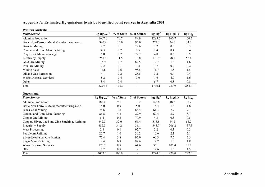
Appendix A 1A

Appendix A: Estimated Hg emissions to air by identified point sources in Australia 2001. Western Australia Point Source kg Hg(tot)

1,2 % of State % of Source kg Hg0 kg Hg(II) kg Hgp Alumina Production 1607.0 70.7 89.9 1285.6 160.7 160.7 Basic Non-Ferrous Metal Manufacturing n.e.c. 340.4 15.0 95.0 272.3 34.0 34.0 Bauxite Mining 2.7 0.1 27.6 2.2 0.3 0.3 Cement and Lime Manufacturing 4.3 0.2 1.5 3.4 0.4 0.4 Clay Brick Manufacturing 5.0 0.2 27.7 4.0 0.5 0.5 Electricity Supply 261.8 11.5 13.8 130.9 78.5 52.4 Gold Ore Mining 15.9 0.7 89.5 12.7 1.6 1.6 Iron Ore Mining 2.2 0.1 7.4 1.7 0.2 0.2 Mining n.e.c. 14.6 0.6 95.5 11.7 1.5 1.5 Oil and Gas Extraction 4.1 0.2 28.5 3.2 0.4 0.4 Waste Disposal Services 8.2 0.4 3.0 1.6 4.9 1.6 Other 8.4 0.4 - 6.7 0.8 0.8 Total 2274.4 100.0 - 1736.1 283.9 254.4 Queensland Point Source kg Hg(tot)

1,2 % of State % of Source kg Hg0 kg Hg(II) kg Hgp Alumina Production 182.0 9.1 10.2 145.6 18.2 18.2 Basic Non-Ferrous Metal Manufacturing n.e.c. 18.0 0.9 5.0 14.4 1.8 1.8 Black Coal Mining 76.6 3.8 86.4 61.3 7.7 7.7 Cement and Lime Manufacturing 86.8 4.3 29.9 69.4 8.7 8.7 Copper Ore Mining 5.4 0.3 70.9 4.3 0.5 0.5 Copper, Silver, Lead and Zinc Smelting, Refining 642.3 32.0 66.4 513.8 64.2 64.2 Electricity Supply 687.3 34.2 36.1 343.7 206.2 137.5 Meat Processing 2.8 0.1 92.7 2.2 0.3 0.3 Petroleum Refining 20.7 1.0 30.2 16.6 2.1 2.1 Silver-Lead-Zinc Ore Mining 75.4 3.8 97.0 60.3 7.5 7.5 Sugar Manufacturing 18.4 0.9 99.6 14.7 1.8 1.8 Waste Disposal Services 175.7 8.8 64.6 35.1 105.4 35.1 Other 15.7 0.8 - 12.6 1.5 1.5 Total 2007.0 100.0 - 1294.0 426.0 287.0

Appendix A 2A

New South Wales Point Source kg Hg(tot)

1,2 % of State % of Source kg Hg0 kg Hg(II) kg Hgp Basic Iron and Steel Manufacturing 385.4 27.2 99.8 308.3 38.5 38.5 Black Coal Mining 11.9 0.8 13.4 9.5 1.2 1.2 Cement and Lime Manufacturing 68.5 4.8 23.6 54.8 6.8 6.8 Chemical Product Manufacturing n.e.c. 125.0 8.8 100.0 100.0 12.5 12.5 Clay Brick Manufacturing 3.6 0.3 20.1 2.8 0.4 0.4 Copper, Silver, Lead and Zinc Smelting, Refining 110.8 7.8 11.5 88.6 11.1 11.1 Electricity Supply 679.7 48.0 35.7 339.9 203.9 135.9 Glass and Glass Product Manufacturing 4.5 0.3 49.5 3.6 0.4 0.4 Organic Industrial Chemical Manufacturing n.e.c. 4.0 0.3 93.0 3.2 0.4 0.4 Paper Stationery Manufacturing 7.0 0.5 100.0 5.6 0.7 0.7 Petroleum Refining 6.0 0.4 8.7 4.8 0.6 0.6 Other 8.9 0.5 - 7.1 0.9 0.9 Total 1415.1 100.0 - 928.2 277.5 209.5 Victoria Point Source kg Hg(tot)

1,2 % of State % of Source kg Hg0 kg Hg(II) kg Hgp Aluminium Smelting 4.8 1.2 90.6 3.8 0.5 0.5 Cement and Lime Manufacturing 5.1 1.2 1.7 4.0 0.5 0.5 Clay Brick Manufacturing 3.5 0.9 19.5 2.8 0.3 0.3 Electricity Supply 266.7 65.5 14.0 133.3 80.0 53.3 Glass and Glass Product Manufacturing 2.3 0.6 24.9 1.8 0.2 0.2 Inorganic Industrial Chemical Manufacturing n.e.c. 70.1 17.2 99.6 49.1 21.0 0.0 Oil and Gas Extraction 2.4 0.6 16.9 1.9 0.2 0.2 Petroleum Refining 39.0 9.6 56.9 31.2 3.9 3.9 Other 13.5 2.9 - 10.9 1.4 1.4 Total 407.4 100.0 - 238.9 108.1 60.4

Appendix A 3A

Tasmania

Point Source kg Hg(tot)1,2 % of State % of Source kg Hg0 kg Hg(II) kg Hgp

Cement and Lime Manufacturing 121.8 40.5 41.9 97.4 12.2 12.2 Copper, Silver, Lead and Zinc Smelting, Refining 92.3 30.7 9.5 73.8 9.2 9.2 Dairy Product Manufacturing n.e.c. 65.0 21.6 98.5 52.0 6.5 6.5 Pulp, Paper and Paperboard Manufacturing 16.9 5.6 61.8 13.5 1.7 1.7 Other 4.9 1.6 - 3.9 0.5 0.5 Total 300.9 100.0 - 240.7 30.1 30.1 South Australia Point Source kg Hg(tot)

1,2 % of State % of Source kg Hg0 kg Hg(II) kg Hgp Cement and Lime Manufacturing 4.0 2.3 1.4 3.2 0.4 0.4 Clay Brick Manufacturing 4.6 2.6 25.7 3.7 0.5 0.5 Copper, Silver, Lead and Zinc Smelting, Refining 120.0 68.4 12.4 96.0 12.0 12.0 Electricity Supply 5.6 3.2 0.3 2.8 1.7 1.1 Iron Ore Mining 27.0 15.4 92.5 21.6 2.7 2.7 Oil and Gas Extraction 4.1 2.3 28.9 3.2 0.4 0.4 Pulp, Paper and Paperboard Manufacturing 7.2 4.1 26.3 5.8 0.7 0.7 Other 3.0 0.7 - 2.4 0.3 0.3 Total 175.5 100.0 - 138.7 18.7 18.1 Australian Capital Territory Point Source kg Hg(tot)

1,2 % of State % of Source kg Hg0 kg Hg(II) kg Hgp Waste Disposal Services 87.46 100 32.2 17.5 52.5 17.5 Total 87.46 100 - 17.5 52.5 17.5

Appendix A 4A

Northern Territory Point Source kg Hg(tot)

1,2 % of State % of Source kg Hg0 kg Hg(II) kg Hgp Bauxite Mining 6.0 17.8 60.6 4.8 0.6 0.6 Hospitals (Except Psychiatric Hospitals) 19.9 59.1 97.0 0.4 14.5 5.0 Oil and Gas Extraction 2.2 6.4 15.3 1.7 0.2 0.2 Plaster Product Manufacturing 3.0 8.9 100.0 2.4 0.3 0.3 Other 2.6 7.8 - 2.0 0.3 0.3 Total 33.7 100.0 - 11.4 15.9 6.3 1 Data from NPI (2003a). 2 Sources that emit 2 kg/yr or less are summed in the category "Other".

Appendix B B 1

APPENDIX B Estimation of Hg emission from sources related to the Pacyna and Pacyna (2002) study Source category Production

Tonnes/yr Emission factor for Hgtot

g/t producedd Total emission

tonnes/yr NPI Point emission

tonnes/yre Non-ferrous metal productiona: - Cu 687 000 5.6 3.85 - Pb 300 000 3.0 0.9 - Zn 684 000 7.6 5.2 Total Non-Ferrous - - 9.95 1.33 Pig iron and steel productionb 7 012 000 0.04 0.28 0.36 Cement productionc 8 438 000 0.1 0.84 0.29 Total 11.07 1.98

a The production figures are from ABS, 2002. Manufacturing production (8301.0). March Quarter, 2002. www.abs.gov.au The EF applied for the smelter emissions in Europe/North America/Australia are lower than smelters in Asia/Africa/South America due to the assumption that more advanced control equipment is in place in the developed countries. b The production figure is from the Department of Industry, Tourism and Resources. www.industry.gov.au c The production figure is from ABS, 2002. Manufacturing production (8301.0). March Quarter, 2002. www.abs.gov.au d From Pacyna and Pacyna, 2002. e From NPI, 2003a.

Appendix C C -1

APPENDIX C

Input data to TAPM Run 10g Run 20 Run 30 Stack Exit Stack Exit Stack Exit

Hg(tot)a Hg0 Hg(II)/Hgp Latitudea Longitudea height Temperature velocity height Temperature velocity height Temperature velocity

No. Facility Name kg/yr kg/yr kg/yr Decimal degrees Decimal degrees m °K m/s m °K m/s m °K m/s

2 Mount Piper PS 45 22.5 22.5 -33.3554 150.0512 250 403 23 3 Liddell PS 46 23 23 -32.3719 150.9783 168 396 22.2 4 Bayswater PS 300 150 150 -32.3940 150.9500 250 403 23 5 Comsteelb 282 226 56 -32.8901 151.7263 10 373 15 10 373 15 50 373 15 6 Pasminco CCSc 110 88 22 -32.9465 151.6236 74 373 15 10 373 15 74 373 15 7 Vales Point PS 86 43 43 -33.1611 151.5417 178 384 20 8 Eraring PS 164 82 82 -33.0623 151.5214 200 403 23 9 Maldon CWd 23 18 5 -34.1898 150.6345 10 373 15 10 373 15 50 373 15

10 BHP Steel PKWe 102 82 20 -34.4634 150.8877 10 373 15 10 373 15 50 373 15 11 Orica Chlorine Pf 124 87 37 -33.9561 151.2209 10 373 15 10 373 15 50 373 15

a From NPI, 2003a. PS - Power Station b Basic Iron/Steel Manuf. c Cu, Ag, Pb, Zn Smelt/Ref. g Data from PS as well as the stack height of Pasminco are provided by CSIRO - EnergyTechnology - Newcastle, NSW. The rest of the data in respective Run is based on assumptions. Grid Centre Coordinates for Run 10: Lat. -31deg 15 min Long.:150 deg 50.5min Grid Centre Coordinates for Run 20 and 30: Lat. -33 deg 39.5 min Long.:150 deg 49.5min

Appendix D D-1

APPENDIX D Simulation: Run 10 (Inner domain) Dry deposition of Hg0 (Inner domain)

Run 10 Total 7.5*7.5 km 12.5*12.5 km 27.5*27.5 km 47.5*47.5 km

Emission Emission Dry Dep Dry Dep Dry Dep Dry Dep Dry Dep Dry Dep Dry Dep Dry Dep Dry Dep Dry Dep Dry Dep Dry Dep

source g/h ug/h g/h % ug/h g/h % ug/h g/h % ug/h g/h %

Mount Piper PS 5.14 389 0.0004 0.01 1019 0.0010 0.02 4597 0.0046 0.09 13698 0.0137 0.27 Bayswater/Lidell PS 39.58 N/A N/A N/A 2590 0.0026 0.01 9622 0.0096 0.02 24651 0.0247 0.06

Comsteel 32.19 26092 0.0261 0.08 42693 0.0427 0.13

Pasminco CCS 12.57 11178 0.0112 0.09 26750 0.0267 0.21 167638 0.1676 0.23 Vales Point PS 9.82 2250 0.0022 0.02 6128 0.0061 0.06 Eraring PS 18.72 3277 0.0033 0.02 9050 0.0090 0.05 Maldon CW 2.63 2757 0.0028 0.11 6077 0.0061 0.23 22628 0.0226 0.86 N/A N/A N/A BHP Steel PKW 11.64 N/A N/A N/A N/A N/A N/A N/A N/A N/A N/A N/A N/A Orica Chlorine P 14.16 11433 0.0114 0.08 17849 0.0178 0.13 37013 0.0370 0.26 64916 0.0649 0.46

The first column within each area is derived from the post-processing of hourly simulated grid concentrations from TAPM. Source BHP Steel PKW is not included in the grid domain. Since sources: Comsteel, Pasminco CCS, Vales Point PS, and Eraring PS are located close to each other, some of the grid cells are overlappning when the deposition rate is calculated for the area 12.5*12.5 km. Dry deposition of Hg(II)/Hgp (Inner domain)

Run 10 Total 7.5*7.5 km 12.5*12.5 km 27.5*27.5 km 47.5*47.5 km

Emission Emission Dry Dep Dry Dep Dry Dep Dry Dep Dry Dep Dry Dep Dry Dep Dry Dep Dry Dep Dry Dep Dry Dep Dry Dep

source g/h ug/h g/h % ug/h g/h % ug/h g/h % ug/h g/h %

Mount Piper PS 5.14 3810 0.0038 0.07 9522 0.0095 0.19 39798 0.0398 0.77 111696 0.1117 2.17 Bayswater/Lidell PS 39.58 N/A N/A N/A 29111 0.0291 0.07 85267 0.0853 0.22 182321 0.1823 0.46

Comsteel 32.19 108635 0.1086 0.34 178011 0.1780 0.55

Pasminco CCS 12.57 46995 0.0470 0.37 112549 0.1125 0.90 747696 0.7477 1.02 Vales Point PS 9.82 11747 0.0117 0.12 31395 0.0314 0.32 Eraring PS 18.72 17063 0.0171 0.09 45183 0.0452 0.24 Maldon CW 2.63 13603 0.0136 0.52 31168 0.0312 1.19 121573 0.1216 4.63 N/A N/A N/A BHP Steel PKW 11.64 N/A N/A N/A N/A N/A N/A N/A N/A N/A N/A N/A N/A Orica Chlorine P 14.16 5418 0.0054 0.04 75481 0.0755 0.53 219977 0.2200 1.55 402499 0.4025 2.84 N/A - Not Available, a term, which is used in this appendix, when the deposition rate has not been able to be derived from TAPM. The reason for this may be that (i) the sources are located to close to each other which makes it difficult to distinguish the deposition fluxes apart, (ii) the source/sources is/are located close to the domain border.

Sources 5,6,7, and 8 is included in this area

Sources 5,6,7, and 8 is included in this area

Appendix D D-2

Simulation: Run 10 (Outer domain) Dry deposition of Hg0 (Outer domain)

Run 10 Total 22.5*22.5 km 37.5*37.5 km 52.5*52.5 km 82.5*82.5 km

Emission Emission Dry Dep Dry Dep Dry Dep Dry Dep Dry Dep Dry Dep Dry Dep Dry Dep Dry Dep Dry Dep Dry Dep Dry Dep

source g/h ug/h g/h % ug/h g/h % ug/h g/h % ug/h g/h %

Mount Piper PS 5.14 3665 0.0037 0.07 9948 0.0099 0.19 19576 0.0196 0.38 50032 0.0500 0.97 Bayswater/Lidell PS 39.58 7896 0.0079 0.02 17855 0.0179 0.05 31093 0.0311 0.08 Comsteel 32.19 N/A N/A N/A Pasminco CCS 12.57 N/A N/A N/A 188696 0.1887 0.26 265088 0.2651 0.36 Vales Point PS 9.82 N/A N/A N/A Eraring PS 18.72 N/A N/A N/A Maldon CW 2.63 16879 0.0169 0.64 38436 0.0384 1.46 N/A N/A N/A N/A N/A N/A BHP Steel PKW 11.64 31472 0.0315 0.27 55793 0.0558 0.48 N/A N/A N/A N/A N/A N/A Orica Chlorine P 14.16 23464 0.0235 0.17 47017 0.0470 0.33 72794 0.0728 0.51 N/A N/A N/A The first column within each area is derived from the post-processing of hourly simulated grid concentrations from TAPM. Source BHP Steel PKW and Orica Chlorine P are located close to each other and some of their gridcells are overlapping in the area 37.7*37.5 km.

Dry deposition of Hg(II)/Hgp (Outer domain)

Run 10 Total 22.5*22.5 km 37.5*37.5 km 52.5*52.5 km 82.5*82.5 km

Emission Emission Dry Dep Dry Dep Dry Dep Dry Dep Dry Dep Dry Dep Dry Dep Dry Dep Dry Dep Dry Dep Dry Dep Dry Dep

source g/h ug/h g/h % ug/h g/h % ug/h g/h % ug/h g/h %

Mount Piper PS 5.14 28672 0.0287 0.56 73606 0.0736 1.43 140591 0.1406 2.74 348201 0.3482 6.78 Bayswater/Lidell PS 39.58 78605 0.0786 0.20 153041 0.1530 0.39 243134 0.2431 0.61 N/A N/A N/A Comsteel 32.19 N/A N/A N/A Pasminco CCS 12.57 N/A N/A N/A 842348 0.8423 1.15 1218264 1.2183 1.66 Vales Point PS 9.82 N/A N/A N/A Eraring PS 18.72 N/A N/A N/A Maldon CW 2.63 87598 0.0876 3.34 207862 0.2079 7.92 N/A N/A N/A N/A N/A N/A BHP Steel PKW 11.64 140024 0.1400 1.20 260964 0.2610 2.24 N/A N/A N/A N/A N/A N/A Orica Chlorine P 14.16 161220 0.1612 1.14 315565 0.3156 2.23 474383 0.4744 3.35 N/A N/A N/A N/A-Not available

Sources 5,6,7, and 8 is included in this area

Sources 5,6,7, and 8 is included in this area

Appendix D D-3

Simulation: Run 20 (Inner domain) Dry deposition of Hg0 (Inner domain)

Run 20 Total 7.5*7.5 km 12.5*12.5 km 27.5*27.5 km 47.5*47.5 km Emission Emission Dry Dep Dry Dep Dry Dep Dry Dep Dry Dep Dry Dep Dry Dep Dry Dep Dry Dep Dry Dep Dry Dep Dry Dep

source g/h ug/h g/h % ug/h g/h % ug/h g/h % ug/h g/h %

Comsteel 32.19 26516 0.0265 0.08 40741 0.0407 0.13 75531 0.0755 0.23 113272 0.1133 0.35 Pasminco CCS 12.57 35320 0.0353 0.28 41019 0.0410 0.33 55226 0.0552 0.44 70906 0.0709 0.56 Maldon CW 2.63 2204 0.0022 0.08 4156 0.0042 0.16 13082 0.0131 0.50 30287 0.0303 1.15 BHP Steel PKW 11.64 9151 0.0092 0.08 14962 0.0150 0.13 30661 0.0307 0.26 48857 0.0489 0.42 Orica Chlorine P 14.16 13077 0.0131 0.09 19514 0.0195 0.14 37296 0.0373 0.26 61684 0.0617 0.44 The first column within each area is derived from the post-processing of hourly simulated grid concentrations from TAPM.

Dry deposition of Hg(II)/Hgp (Inner domain) Run 20 Total 7.5*7.5 km 12.5*12.5 km 27.5*27.5 km 47.5*47.5 km

Emission Emission Dry Dep Dry Dep Dry Dep Dry Dep Dry Dep Dry Dep Dry Dep Dry Dep Dry Dep Dry Dep Dry Dep Dry Dep source g/h ug/h g/h % ug/h g/h % ug/h g/h % ug/h g/h %

Comsteel 32.19 110162 0.1102 0.34 169252 0.1693 0.53 313761 0.3138 0.97 470456 0.4705 1.46 Pasminco CCS 12.57 141592 0.1416 1.13 173167 0.1732 1.38 N/A N/A N/A N/A N/A N/A Maldon CW 2.63 10257 0.0103 0.39 20312 0.0203 0.77 68870 0.0689 2.62 167349 0.1673 6.37 BHP Steel PKW 11.64 20374 0.0204 0.17 26478 0.0265 0.23 N/A N/A N/A N/A N/A N/A Orica Chlorine P 14.16 92717 0.0927 0.66 137442 0.1374 0.97 256474 0.2565 1.81 408345 0.4083 2.88 N/A - Not Available

Appendix D D-4

Simulation: Run 20 (Outer domain) Dry deposition of Hg0 (Outer domain)

Run 20 Total 22.5*22.5 km 37.5*37.5 km 52.5*52.5 km 82.5*82.5 km Emission Emission Dry Dep Dry Dep Dry Dep Dry Dep Dry Dep Dry Dep Dry Dep Dry Dep Dry Dep Dry Dep Dry Dep Dry Dep

source g/h ug/h g/h % ug/h g/h % ug/h g/h % ug/h g/h %

Comsteel 32.19 65427 0.0654 0.20 99187 0.0992 0.31 177992 0.1780 0.55 257581 0.2576 0.80 Pasminco CCS 12.57 25500 0.0255 0.20 38591 0.0386 0.31 69458 0.0695 0.55 100098 0.1001 0.80 Maldon CW 2.63 10373 0.0104 0.40 21728 0.0217 0.83 N/A N/A N/A N/A N/A N/A BHP Steel PKW 11.64 27555 0.0276 0.24 43111 0.0431 0.37 86999 0.0870 0.75 141428 0.1414 1.21 Orica Chlorine P 14.16 29704 0.0297 0.21 48308 0.0483 0.34 N/A N/A N/A N/A N/A N/A The first column within each area is derived from the post-processing of hourly simulated grid concentrations from TAPM. N/A - Not Available

Dry deposition of Hg(II)/Hgp (Outer domain) Run 20 Total 22.5*22.5 km 37.5*37.5 km 52.5*52.5 km 82.5*82.5 km

Emission Emission Dry Dep Dry Dep Dry Dep Dry Dep Dry Dep Dry Dep Dry Dep Dry Dep Dry Dep Dry Dep Dry Dep Dry Dep source g/h ug/h g/h % ug/h g/h % ug/h g/h % ug/h g/h %

Comsteel 32.19 300386 0.3004 0.93 445736 0.4457 1.38 770047 0.7700 2.39 1101919 1.1019 3.42 Pasminco CCS 12.57 117213 0.1172 0.93 186249 0.1862 1.48 392031 0.3920 3.12 694447 0.6944 5.52 Maldon CW 2.63 53229 0.0532 2.03 117984 0.1180 4.49 N/A N/A N/A N/A N/A N/A BHP Steel PKW 11.64 125202 0.1252 1.08 204637 0.2046 1.76 458433 0.4584 3.94 885500 0.8855 7.60 Orica Chlorine P 14.16 148421 0.1484 1.05 282652 0.2827 2.00 N/A N/A N/A N/A N/A N/A N/A - Not Available

Appendix D D-5

Simulation: Run 30 (Inner domain) Dry deposition of Hg0 (Inner domain)

Run 30 Total 7.5*7.5 km 12.5*12.5 km 27.5*27.5 km 47.5*47.5 km Emission Emission Dry Dep Dry Dep Dry Dep Dry Dep Dry Dep Dry Dep Dry Dep Dry Dep Dry Dep Dry Dep Dry Dep Dry Dep

source g/h ug/h g/h % ug/h g/h % ug/h g/h % ug/h g/h %

Comsteel 32.19 12734 0.0127 0.04 21255 0.0213 0.07 45513 0.0455 0.14 74930 0.0749 0.23 Pasminco CCS 12.57 5860 0.0059 0.05 8305 0.0083 0.07 15567 0.0156 0.12 25286 0.0253 0.20 Maldon CW 2.63 1250 0.0012 0.05 2681 0.0027 0.10 10126 0.0101 0.39 25842 0.0258 0.98 BHP Steel PKW 11.64 3066 0.0031 0.03 6238 0.0062 0.05 16344 0.0163 0.14 30125 0.0301 0.26 Orica Chlorine P 14.16 5453 0.0055 0.04 9453 0.0095 0.07 22373 0.0224 0.16 42430 0.0424 0.30 The first column within each area is derived from the post-processing of hourly simulated grid concentrations from TAPM. N/A - Not Available

Dry deposition of Hg(II)/Hgp (Inner domain) Run 30 Total 7.5*7.5 km 12.5*12.5 km 27.5*27.5 km 47.5*47.5 km

Emission Emission Dry Dep Dry Dep Dry Dep Dry Dep Dry Dep Dry Dep Dry Dep Dry Dep Dry Dep Dry Dep Dry Dep Dry Dep source g/h ug/h g/h % ug/h g/h % ug/h g/h % ug/h g/h %

Comsteel 32.19 52898 0.0529 0.16 88295 0.0883 0.27 189033 0.1890 0.59 311127 0.3111 0.97 Pasminco CCS 12.57 24369 0.0244 0.19 33288 0.0333 0.26 N/A N/A N/A N/A N/A N/A Maldon CW 2.63 6256 0.0063 0.24 14101 0.0141 0.54 56146 0.0561 2.14 147331 0.1473 5.61 BHP Steel PKW 11.64 6307 0.0063 0.05 10126 0.0101 0.09 N/A N/A N/A N/A N/A N/A Orica Chlorine P 14.16 38219 0.0382 0.27 65501 0.0655 0.46 149888 0.1499 1.06 271773 0.2718 1.92 N/A - Not Available

Appendix D D-6

Simulation: Run 30 (Outer domain)

Dry deposition of Hg0 (Outer domain) Run 30 Total 22.5*22.5 km 37.5*37.5 km 52.5*52.5 km 82.5*82.5 km

Emission Emission Dry Dep Dry Dep Dry Dep Dry Dep Dry Dep Dry Dep Dry Dep Dry Dep Dry Dep Dry Dep Dry Dep Dry Dep source g/h ug/h g/h % ug/h g/h % ug/h g/h % ug/h g/h %

Comsteel 32.19 36261 0.0363 0.11 60461 0.0605 0.19 125672 0.1257 0.39 198303 0.1983 0.62 Pasminco CCS 12.57 11284 0.0113 0.09 19020 0.0190 0.15 41146 0.0411 0.33 66823 0.0668 0.53 Maldon CW 2.63 7490 0.0075 0.29 17367 0.0174 0.66 N/A N/A N/A N/A N/A N/A BHP Steel PKW 11.64 15683 0.0157 0.13 26943 0.0269 0.23 61583 0.0616 0.53 112537 0.1125 0.97 Orica Chlorine P 14.16 17340 0.0173 0.12 31921 0.0319 0.23 N/A N/A N/A N/A N/A N/A The first column within each area is derived from the post-processing of hourly simulated grid concentrations from TAPM. N/A - Not Available

Dry deposition of Hg(II)/Hgp (Outer domain) Run 30 Total 22.5*22.5 km 37.5*37.5 km 52.5*52.5 km 82.5*82.5 km

Emission Emission Dry Dep Dry Dep Dry Dep Dry Dep Dry Dep Dry Dep Dry Dep Dry Dep Dry Dep Dry Dep Dry Dep Dry Dep source g/h ug/h g/h % ug/h g/h % ug/h g/h % ug/h g/h %

Comsteel 32.19 171009 0.1710 0.53 278027 0.2780 0.86 549930 0.5499 1.71 851505 0.8515 2.65 Pasminco CCS 12.57 57770 0.0578 0.46 104283 0.1043 0.83 273613 0.2736 2.18 555814 0.5558 4.42 Maldon CW 2.63 40414 0.0404 1.54 97526 0.0975 3.71 N/A N/A N/A N/A N/A N/A BHP Steel PKW 11.64 81889 0.0819 0.70 145499 0.1455 1.25 370325 0.3703 3.18 767352 0.7674 6.59 Orica Chlorine P 14.16 91785 0.0918 0.65 185480 0.1855 1.31 N/A N/A N/A N/A N/A N/A N/A - Not Available

CONTACT DETAILS

Christian Peterson Graduate School of the Environment

Macquarie University NSW 2109, Australia

Ph 02 9850 7988 Fax 02 9850 7972 Email: director@gse.mq.edu.au

Professor Peter Nelson

Graduate School of the Environment Macquarie University NSW 2109, Australia

Ph 02 9850 6958 Fax 02 9850 7972

Email: peter.nelson@gse.mq.edu.au

Anthony Morrison Graduate School of the Environment

Macquarie University NSW 2109, Australia

Ph 02 9850 7869 Fax 02 9850 7972

Email: tony.morrison@gse.mq.edu.au